1

DEPARTMENT OF ECONOMICS

ISSN 1441-5429

DISCUSSION PAPER 25/14

The Effect of Military Expenditure on Growth: An Empirical Synthesis1

Sefa Awaworyi2 and Siew Ling Yew

3

Abstract Using a sample of 243 meta-observations drawn from 42 primary studies, this paper conducts a

metaanalysis of the empirical literature that examines the impact of military expenditure on

economic growth. We find that existing studies indicate growth-retarding effects of military

expenditure. The results from the meta-regression analysis suggest that the effect size estimate is

strongly influenced by study variations. Specifically, we find that underlying theoretical models,

econometric specifications, and data type as well as data period are relevant factors that explain the

heterogeneity in the military expenditure-growth literature. Results also show that positive effects

of military expenditure on growth are more pronounced for developed countries than less developed

countries.

1 Preliminary draft; comments are welcome

2 Corresponding Author Email: sefa.awaworyi@monash.edu Department of Economics, Monash University, VIC 3800,

Australia 3 Email: siew.ling.yew@monash.edu Department of Economics, Monash University, VIC 3800, Australia

© 2014 Sefa Awaworyi and Siew Ling Yew

All rights reserved. No part of this paper may be reproduced in any form, or stored in a retrieval system, without the prior written

permission of the author.

2

1. Introduction

Though it is not always the case, economic development is often accompanied by a rise in military

expenditure (hereafter ME). For instance, data from World Bank (World Development Indicators) shows

that from 1988 to 2012, countries with the highest ME (as a proportion of GDP) have the highest

economic development (5.96% in high income non-OECD and 2.57% in OECD), while countries with

lower shares have lower economic development (2.08% in middle income countries and 2.05% in low

income countries). What is the interaction between ME and economic development? Does ME promote

economic growth? There are no clear-cut answers to these questions as complex interactions between

ME and economic growth may occur.

Theoretically, ME can promote as well as hinder growth. ME may promote growth through the

following channels. ME develops new technology that spills over to private sector, creates

socioeconomic structure through spin-offs effects, provides public infrastructure and protections against

threats, and increases aggregate demand and employment through the Keynesian multiplier effect. On

the other hand, ME is harmful for growth through its opportunity costs. Through the gun-butter trade-

off, ME crowds out investment or other productive activities. A rise in ME often comes with increased

tax burden and government debt which may reduce growth. The net effect of ME on growth therefore

will depend on the benefits versus the opportunity costs.

Although many studies have investigated the relationship between ME and growth,

unfortunately, the empirical evidence that is currently available is inconclusive (Smith, 1980; Yildirim et

al., 2005). Some studies show that ME is conducive to growth (see e.g., Benoit 1973, 1978; Weede,

1983; Biswas, 1993; Cohen et al., 1996; Yakovlev, 2007), some other studies however show that ME may

retard growth (see e.g., Deger and Smith, 1983; Faini et al., 1984; Deger, 1986; Mintz and Huang, 1990,

1991; Heo, 1999; Ward and Davis, 1992; Pieroni, 2009a). There are also studies that show ME neither

hinders nor boosts growth (see e.g., Biswas and Ram, 1986; Alexander, 1990).

According to Smith (1992), and Mintz and Stevenson (1995), theoretical and methodological

limitations are possible reasons for the failure to reach a consensus in the literature. Furthermore, the

heterogeneity in the reported findings has often been associated with the use of different samples,

different theoretical and econometric specification, and different time periods (Chen et al., 2014).

Our goal in this paper is to provide a synthesis of the empirical literature that examines the

effects of ME on growth using meta-analysis techniques. Based on 42 primary studies with 243

estimates, we formulate five hypotheses (H1-H5) to investigate the military expenditure-growth

(hereafter ME-G), relationship: (H1) ME as a proportion of GDP reduces growth, (H2) ME as a proportion

3

of GDP reduces growth in less developed countries (LDCs), (H3) ME as a proportion of GDP increases

growth, (H4) The effect of ME as a proportion of GDP on growth is non-linear, and (H5) ME as a

proportion of GDP increases growth in developed countries.

Our study re-examines and extends the work by Alptekin and Levine (2012), hereafter A-L, who

conduct a meta-analysis of 32 studies on the ME-G relationship by formulating the first four hypotheses

(H1)-(H4) mentioned earlier. Our study validates the results by A-L after using a subset of the 32 primary

studies that they included in their meta-analysis. In addition, by using a larger set of primary studies,

which includes newly published studies, we find that the general conclusion of A-L, that is the positive

effect of ME on growth, is no longer valid.

Unlike A-L, we split our meta-observations into three country types – developed countries, LDCs

and mixed countries, in order to thoroughly investigate the ME-G relationship listed in the hypotheses

(H1)-(H5). A-L test (H2) by introducing a dummy which captures the effect of studies that report

estimates on Africa. Beyond this approach, we run a separate meta-analysis for LDCs only. This enables

us to determine the possible causes of heterogeneity in the literature that examines the ME-G effect for

LDCs only. We use a similar approach to test (H5). In essence, we conduct a meta-analysis using 243

estimates to test (H1) and (H3), and also (H2), (H4) and (H5) (by introducing dummies). To explore (H2)

and (H5) more thoroughly, we use the less-developed-countries sample only (147 estimates) to test

(H2), and the developed-countries sample only (26 estimates) to test (H5).

This study makes a number of important contributions: first, we examine the ‘genuine’ effect of

ME on growth beyond publication bias. Second, based on various sample clusters which capture country

differences, we provide a generalized conclusion on the effects of ME on growth per development level.

Third, we address issues of between and within study variations and explore possible causes of

systematic heterogeneity in the ME-G literature. Thus, we control for study-to-study variations and

provide an overall net ME-G effect. Lastly, our results lay a foundation and guide future studies into

examining areas of particular importance.

2. Existing Theoretical and Empirical Perspectives

In this section, we provide a brief review of the theoretical foundations and various empirical findings

for the effects of ME on growth.3

Theoretical arguments on the effects of ME on growth may come from three channels: the

supply, the demand, and the security channels. The supply channel considers the opportunity cost of ME

3 See Alptekin and Levine (2012) for an overview of the various econometric approaches that examine the ME-G relationship.

4

(such as the crowding-out effect, an adverse balance of payment, and distortions), and the spill-over or

the spin-off effect of ME (such as the development of new technology and infrastructure by the military

sector that benefits the private sector). On the other hand, the demand channel suggests that ME

increases aggregate demand, employment and capital utilization through the Keynesian multiplier

effect. The security channel stresses the role of ME in providing security for people and properties from

internal and external threats. Theoretically, the net effect of ME on growth is uncertain and thus, how

ME affects growth is ultimately an empirical issue.

Benoit’s famous studies (1973, 1978) find that ME stimulates growth in a sample of 44 LDCs.

According to Benoit, only a small part of income not spent on military is allocated to productive activities

in LDCs. On the other hand, spending on military contributes to growth by providing education, medical

care, technical training, and public infrastructure such as roads, airports and communication networks

which could benefit the private sector. Military forces also engage in scientific and R&D activities which

have positive spill-over effects to private production.

Numerous studies afterwards have focused on validating Benoit’s (1973, 1978) finding.

However, subsequent empirical studies show inconsistent results on the subject. The diversity of results

largely comes from applying different models (such as neoclassical or endogenous growth models and

Keynesian models), and using a variety of specifications, econometric estimators and types of sample in

cross-section, time-series or panels (Dunne et al., 2005).4

Empirical studies such as Kennedy (1983), Weede (1983), Biswas (1993), Mueller and Atesoglu

(1993), Cohen et al. (1996), Brumm (1997), Murdoch et al. (1997), and Yakovlev (2007) support Benoit’s

finding. In particular, Weede (1983), Deger and Sen (1983), Deger (1986), and Yakovlev (2007) find

positive effects of ME on growth through human capital accumulation or spin-off technologies. Kennedy

(1983), DeGrasse (1983), and Mueller and Atesoglu (1993), among others, find that ME helps growth

through the process of enhancing infrastructure, increasing a Keynesian-type aggregate demand, and

promoting full employment.

Studies that permit ME to affect growth through multiple channels such as Deger and Smith

(1983), Faini et al. (1984), Deger (1986), Mintz and Huang (1990, 1991), and Ward and Davis (1992) find

that the net effect of ME is negative. For example, Deger (1986) finds that while ME increases growth

through demand and technological spin-off effects, ME reduces growth through the resource effects by

reducing the savings rate. Many studies also find that ME reduces growth by crowding out private

4 The neoclassical or endogenous growth models focus on the supply-side, while the Keynesian models focus on the demand-

side.

5

investment and increasing tax burden (see e.g., Smith, 1980; Cappelen et al., 1984; Batchelor et al.,

2000; Dunne et al., 2001). These studies imply that there is a substantial trade-off between ME and

resource use (the gun-butter trade off). Higher ME often reduces expenditure that is essential to build

future productive capacities such as investment in new capital stock, health and education.

The extent of the opportunity cost of ME (the gun-butter trade off) will depend on the size of

ME as a proportion of GDP, how the increased ME is financed, the effectiveness of the military sector in

providing security, and whether the country that increases ME is resource-constrained. For instance,

distortionary taxes used to finance ME tend to distort saving decisions and lower growth when taxes are

sufficiently large (Barro, 1990); resource-constrained countries that increase ME at the expense of

cutting development programs such as education and health tend to reduce growth (see, e.g.,

Frederiksen and Looney, 1983).

Another group of studies such as Biswas and Ram (1986), Alexander (1990), Kinsella (1990),

Payne and Ross (1992), Ward et al. (1992), and DeRouen (1994) show that there is no significant

relationship between ME and growth. A more recent study by Pieroni (2009b) shows that there is no

relationship between ME and growth in countries with low ME.

Thus, a priori, ME could have an insignificant, positive or negative effect on growth, as

documented in previous surveys of the military-growth literature (see, e.g., Chan, 1987; Ram, 2003;

Smaldone, 2006; Dunne and Uye, 2009).

3. Data and Methodology

Our meta-analysis methodology draws on guidelines proposed by the meta-analysis of economics

research-network (MAER-NET), which reflects best practices and transparency in meta-analyses (Stanley

et al., 2013). To collect relevant studies that examine the ME-G relationship, we search for journal

articles and working papers in five electronic databases – JSTOR, Business Source Complete, EconLit,

Google Scholar, and ProQuest, which in itself contains over 30 databases. We use various keywords for

ME and growth.5 We also check the references of related studies to ensure that no relevant studies are

excluded from our meta-analysis.

We use the following criteria to select studies for inclusion in our meta-analysis. 1) We include

only the empirical studies that examine the direct effect of ME on growth. 2) ME must be an

5 Keywords for military expenditure include defence (defense) expenditure OR defence (defense) spending OR military spending

OR military expenditure OR defense burden. Keywords for growth include economic growth OR economic development OR GDP

OR gross domestic product.

6

independent variable and be measured as a share of GDP. 3) The growth rate of GDP is the dependent

variable. We leave out studies that use the level of ME, the growth rate of ME and GDP level. We also

include studies that adopt simultaneous equation models but we report only the direct effects as it is

not possible to capture the net effect from these studies. (4) Given that partial correlation coefficients

are calculated to allow for comparability of studies, we exclude studies that satisfy criteria (1) and (2)

but do no report all relevant statistics to enable the calculation of partial correlation coefficients.

Following the above criteria, our meta-analysis therefore includes 42 relevant studies with 243

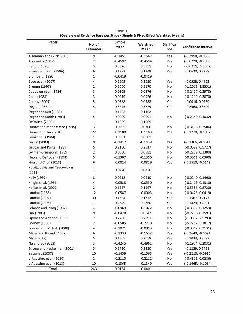
estimates. Table 1 presents an overview of these 42 studies in terms of the reported number of

estimates, their simple means and fixed effects weighted means.

3.1. Partial Correlation Coefficients (PCCs)

To allow for comparability of studies and reported effect-size estimates, we first calculate partial

correlation coefficients (PCCs), which measure the association between ME and per-capita GDP growth

while all other independent variables are held constant. Given that PCCs are independent of the metrics

used in measuring both dependent and independent variables, they are comparable across studies.

However, given that PCCs are based on regression coefficients, there are limitations using PCCs

especially when primary studies do not control for all relevant covariates. If a regression model is mis-

specified, PCC will be biased because it is not based on a regression coefficient that is obtained after

controlling for all relevant variables. Nonetheless, this does not make PCCs irrelevant. We later control

for model specification (i.e., omitted variables) in our meta-regression to examine if the model

specification has any systematic effect on PCCs. An alternative to PCCs is elasticities but primary studies

usually do not report sufficient information for calculating elasticities. Thus, PCCs are very often used in

meta-analysis (see, e.g., Alptekin and Levine, 2012; Ugur, 2013)

For each effect-size estimate reported by primary studies, we calculate a PCC and its associated

standard error in accordance with equations (1) and (2) given below.

√

(1)

and

√

(2)

7

Here, and are PCC and standard errors associated with each effect-size estimate. represents

variation due to sampling error and its inverse is used as weight in the calculation of fixed-effect

weighted averages for each study. and are -value and degrees of freedom associated with

estimates reported in primary studies.

3.2. Fixed Effect Weighted Means

We calculate fixed-effect weighted averages (hereafter, FEEs) for estimates reported in each study. We

provide FEEs as a reliable overview of the ME-G evidence base as they are more reliable than simple

means, and compared to random-effects weighted averages, they are less affected by publication bias

(Henmi and Copas, 2010; Stanley, 2008; Stanley and Doucouliagos, 2014). FEEs are calculated using (3)

below.

∑ (

)

∑

(3)

Here, is the FEE and all other variables remain as explained before. FEEs assign higher

weights to more precise estimates, and vice versa, thus, accounting for within-study variations.

Table 1 reports results from the study-based FEEs. First, based on a subset of our included

studies, which consists of 32 studies included in A-L, we confirm the results presented by A-L to a large

extent (except for very minor variations). FEEs provided by A-L for all 32 studies are consistent with what

we find, except for slight variations in averages reported for Grobar and Porter (1989), and Lipow and

Antinori (1995), where effect sizes are about 0.1 higher than those reported in A-L.

Based on the 42 studies included in this current study, we find that of the 243 reported

estimates, 88 are insignificant, 80 are negative and significant, and 75 are positive and significant. The

average FFE for all 243 estimates is -0.0401. Thus, based on our entire dataset, we conclude that ME has

a negative effect on growth, in contrast to A-L who find a positive relationship. However, drawing on

inferences made by Cohen (1988), our overall average FEE for the ME-G relationship is of no practical

relevance.6 Furthermore, the calculated FEE is valid only if there are no issues of publication selection

bias. Thus, to investigate if the reported FEEs are fraught with issues of publication selection bias, we

conduct various tests in the next subsection.

6 Cohen indicates that an effect size represents a small effect if its absolute value is less than 0.10, a medium effect if it is 0.25

and over, and a large effect if it is greater than 0.4.

8

3.3. Genuine Effects Beyond Bias

FEEs cannot be considered as ‘genuine’ measures of the effect of ME on growth, given that estimates

reported by primary studies are subject to publication selection bias and/or affected by within-study

dependence between reported coefficients (see De Dominicis et al., 2008; Ugur, 2013). Thus, in what

follows, we conduct various tests to examine whether the reported effect-sizes are tainted with

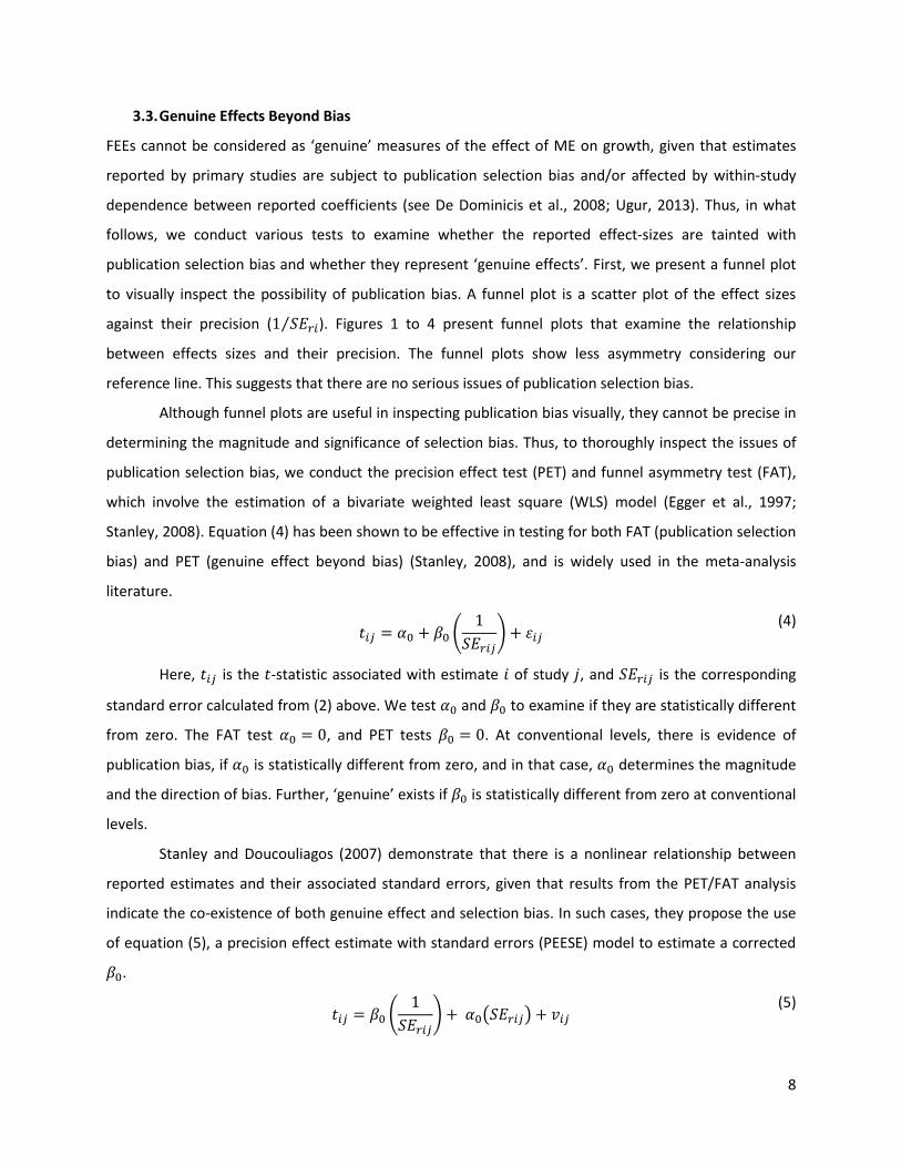
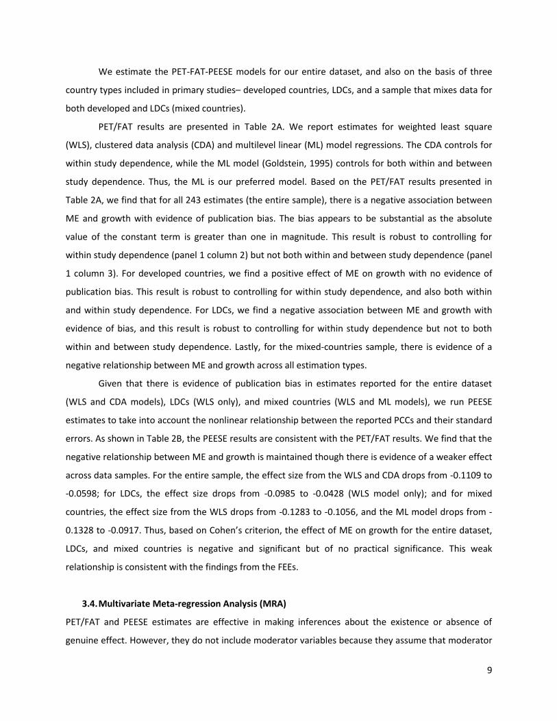
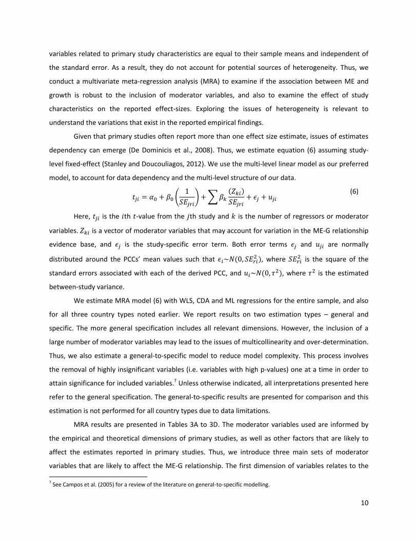
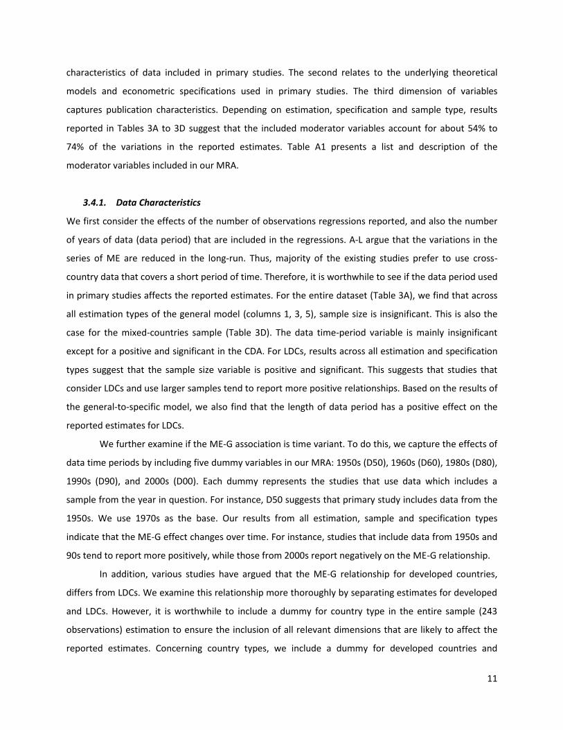
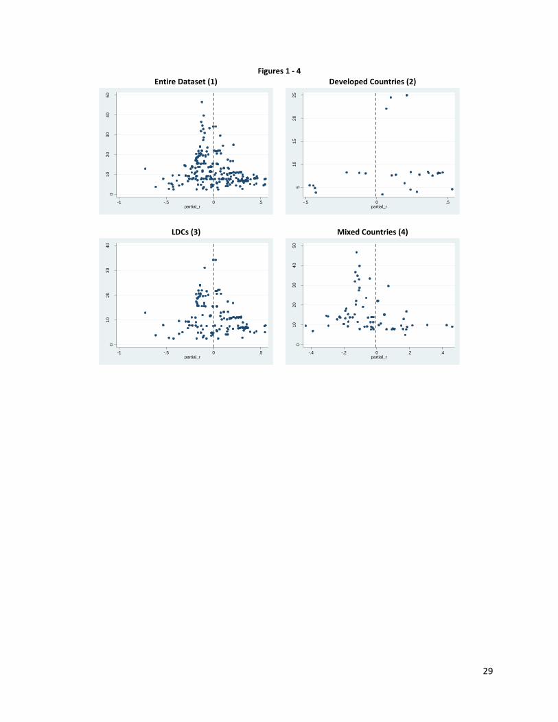
publication selection bias and whether they represent ‘genuine effects’. First, we present a funnel plot

to visually inspect the possibility of publication bias. A funnel plot is a scatter plot of the effect sizes

against their precision ( ⁄ ). Figures 1 to 4 present funnel plots that examine the relationship

between effects sizes and their precision. The funnel plots show less asymmetry considering our

reference line. This suggests that there are no serious issues of publication selection bias.

Although funnel plots are useful in inspecting publication bias visually, they cannot be precise in

determining the magnitude and significance of selection bias. Thus, to thoroughly inspect the issues of

publication selection bias, we conduct the precision effect test (PET) and funnel asymmetry test (FAT),

which involve the estimation of a bivariate weighted least square (WLS) model (Egger et al., 1997;

Stanley, 2008). Equation (4) has been shown to be effective in testing for both FAT (publication selection

bias) and PET (genuine effect beyond bias) (Stanley, 2008), and is widely used in the meta-analysis

literature.

(

)

(4)

Here, is the -statistic associated with estimate of study , and is the corresponding

standard error calculated from (2) above. We test and to examine if they are statistically different

from zero. The FAT test , and PET tests . At conventional levels, there is evidence of

publication bias, if is statistically different from zero, and in that case, determines the magnitude

and the direction of bias. Further, ‘genuine’ exists if is statistically different from zero at conventional

levels.

Stanley and Doucouliagos (2007) demonstrate that there is a nonlinear relationship between

reported estimates and their associated standard errors, given that results from the PET/FAT analysis

indicate the co-existence of both genuine effect and selection bias. In such cases, they propose the use

of equation (5), a precision effect estimate with standard errors (PEESE) model to estimate a corrected

.

(

) ( )

(5)

9

We estimate the PET-FAT-PEESE models for our entire dataset, and also on the basis of three

country types included in primary studies– developed countries, LDCs, and a sample that mixes data for

both developed and LDCs (mixed countries).

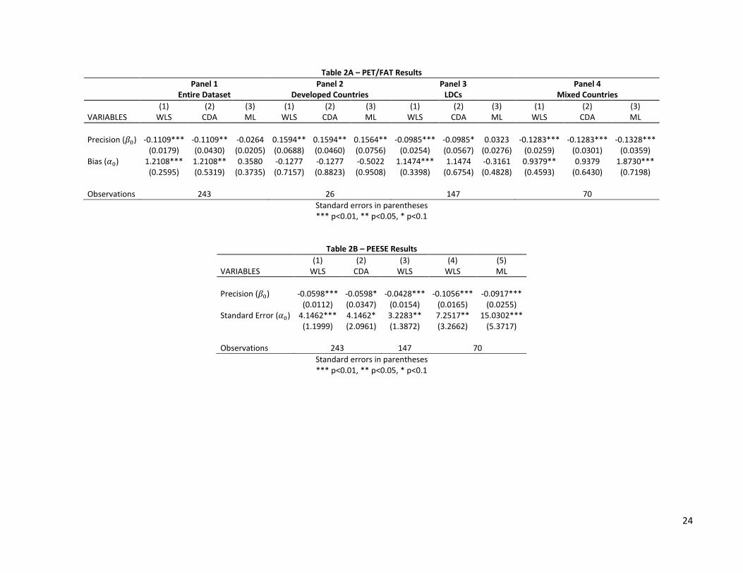
PET/FAT results are presented in Table 2A. We report estimates for weighted least square

(WLS), clustered data analysis (CDA) and multilevel linear (ML) model regressions. The CDA controls for

within study dependence, while the ML model (Goldstein, 1995) controls for both within and between

study dependence. Thus, the ML is our preferred model. Based on the PET/FAT results presented in

Table 2A, we find that for all 243 estimates (the entire sample), there is a negative association between

ME and growth with evidence of publication bias. The bias appears to be substantial as the absolute

value of the constant term is greater than one in magnitude. This result is robust to controlling for

within study dependence (panel 1 column 2) but not both within and between study dependence (panel

1 column 3). For developed countries, we find a positive effect of ME on growth with no evidence of

publication bias. This result is robust to controlling for within study dependence, and also both within

and within study dependence. For LDCs, we find a negative association between ME and growth with

evidence of bias, and this result is robust to controlling for within study dependence but not to both

within and between study dependence. Lastly, for the mixed-countries sample, there is evidence of a

negative relationship between ME and growth across all estimation types.

Given that there is evidence of publication bias in estimates reported for the entire dataset

(WLS and CDA models), LDCs (WLS only), and mixed countries (WLS and ML models), we run PEESE

estimates to take into account the nonlinear relationship between the reported PCCs and their standard

errors. As shown in Table 2B, the PEESE results are consistent with the PET/FAT results. We find that the

negative relationship between ME and growth is maintained though there is evidence of a weaker effect

across data samples. For the entire sample, the effect size from the WLS and CDA drops from -0.1109 to

-0.0598; for LDCs, the effect size drops from -0.0985 to -0.0428 (WLS model only); and for mixed

countries, the effect size from the WLS drops from -0.1283 to -0.1056, and the ML model drops from -

0.1328 to -0.0917. Thus, based on Cohen’s criterion, the effect of ME on growth for the entire dataset,

LDCs, and mixed countries is negative and significant but of no practical significance. This weak

relationship is consistent with the findings from the FEEs.

3.4. Multivariate Meta-regression Analysis (MRA)

PET/FAT and PEESE estimates are effective in making inferences about the existence or absence of

genuine effect. However, they do not include moderator variables because they assume that moderator

10

variables related to primary study characteristics are equal to their sample means and independent of

the standard error. As a result, they do not account for potential sources of heterogeneity. Thus, we

conduct a multivariate meta-regression analysis (MRA) to examine if the association between ME and

growth is robust to the inclusion of moderator variables, and also to examine the effect of study

characteristics on the reported effect-sizes. Exploring the issues of heterogeneity is relevant to

understand the variations that exist in the reported empirical findings.

Given that primary studies often report more than one effect size estimate, issues of estimates

dependency can emerge (De Dominicis et al., 2008). Thus, we estimate equation (6) assuming study-

level fixed-effect (Stanley and Doucouliagos, 2012). We use the multi-level linear model as our preferred

model, to account for data dependency and the multi-level structure of our data.

(

) ∑

( )

(6)

Here, is the th -value from the th study and is the number of regressors or moderator

variables. is a vector of moderator variables that may account for variation in the ME-G relationship

evidence base, and is the study-specific error term. Both error terms and are normally

distributed around the PCCs’ mean values such that ( ), where

is the square of the

standard errors associated with each of the derived PCC, and ( ), where is the estimated

between-study variance.

We estimate MRA model (6) with WLS, CDA and ML regressions for the entire sample, and also

for all three country types noted earlier. We report results on two estimation types – general and

specific. The more general specification includes all relevant dimensions. However, the inclusion of a

large number of moderator variables may lead to the issues of multicollinearity and over-determination.

Thus, we also estimate a general-to-specific model to reduce model complexity. This process involves

the removal of highly insignificant variables (i.e. variables with high p-values) one at a time in order to

attain significance for included variables.7 Unless otherwise indicated, all interpretations presented here

refer to the general specification. The general-to-specific results are presented for comparison and this

estimation is not performed for all country types due to data limitations.

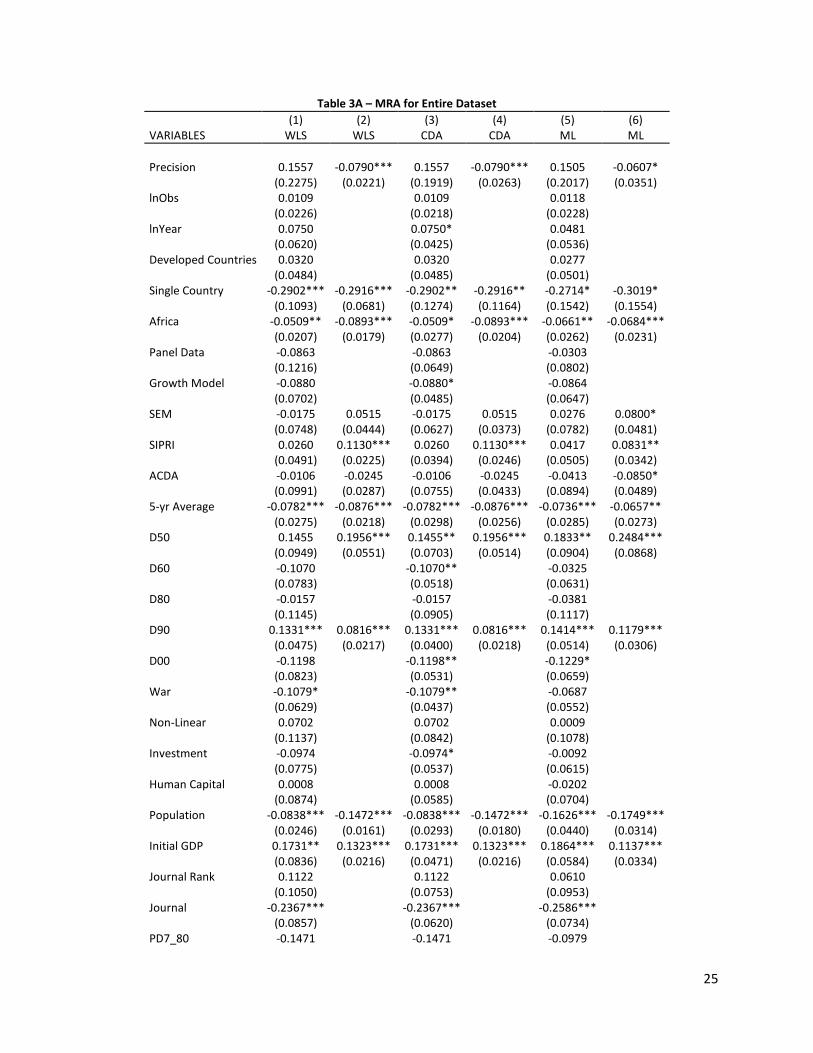
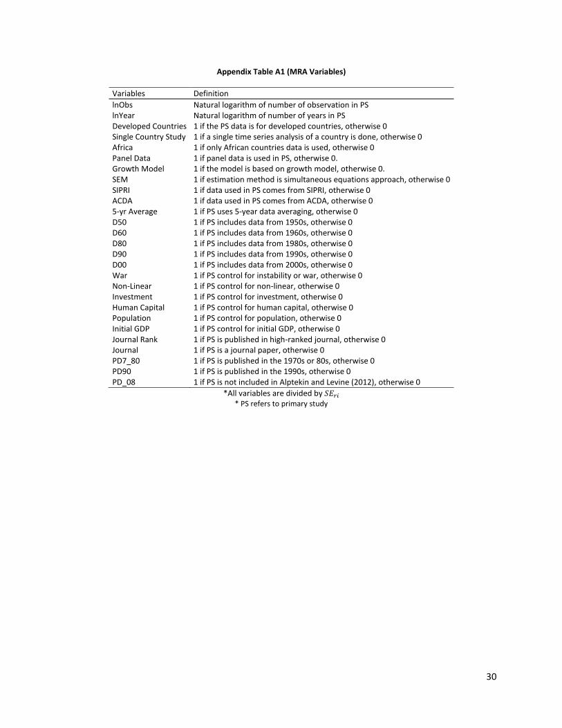
MRA results are presented in Tables 3A to 3D. The moderator variables used are informed by

the empirical and theoretical dimensions of primary studies, as well as other factors that are likely to

affect the estimates reported in primary studies. Thus, we introduce three main sets of moderator

variables that are likely to affect the ME-G relationship. The first dimension of variables relates to the

7 See Campos et al. (2005) for a review of the literature on general-to-specific modelling.

11

characteristics of data included in primary studies. The second relates to the underlying theoretical

models and econometric specifications used in primary studies. The third dimension of variables

captures publication characteristics. Depending on estimation, specification and sample type, results

reported in Tables 3A to 3D suggest that the included moderator variables account for about 54% to

74% of the variations in the reported estimates. Table A1 presents a list and description of the

moderator variables included in our MRA.

3.4.1. Data Characteristics

We first consider the effects of the number of observations regressions reported, and also the number

of years of data (data period) that are included in the regressions. A-L argue that the variations in the

series of ME are reduced in the long-run. Thus, majority of the existing studies prefer to use cross-

country data that covers a short period of time. Therefore, it is worthwhile to see if the data period used

in primary studies affects the reported estimates. For the entire dataset (Table 3A), we find that across

all estimation types of the general model (columns 1, 3, 5), sample size is insignificant. This is also the

case for the mixed-countries sample (Table 3D). The data time-period variable is mainly insignificant

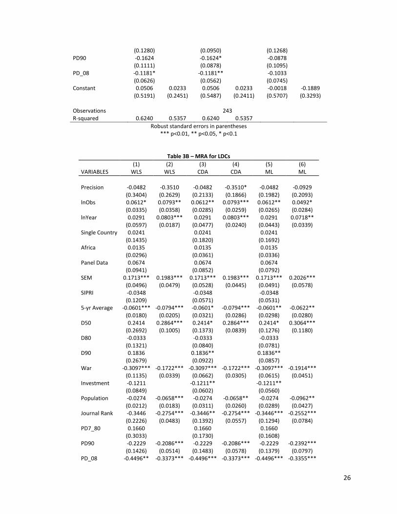
except for a positive and significant in the CDA. For LDCs, results across all estimation and specification

types suggest that the sample size variable is positive and significant. This suggests that studies that

consider LDCs and use larger samples tend to report more positive relationships. Based on the results of

the general-to-specific model, we also find that the length of data period has a positive effect on the

reported estimates for LDCs.

We further examine if the ME-G association is time variant. To do this, we capture the effects of

data time periods by including five dummy variables in our MRA: 1950s (D50), 1960s (D60), 1980s (D80),

1990s (D90), and 2000s (D00). Each dummy represents the studies that use data which includes a

sample from the year in question. For instance, D50 suggests that primary study includes data from the

1950s. We use 1970s as the base. Our results from all estimation, sample and specification types

indicate that the ME-G effect changes over time. For instance, studies that include data from 1950s and

90s tend to report more positively, while those from 2000s report negatively on the ME-G relationship.

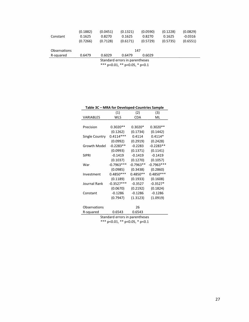
In addition, various studies have argued that the ME-G relationship for developed countries,

differs from LDCs. We examine this relationship more thoroughly by separating estimates for developed

and LDCs. However, it is worthwhile to include a dummy for country type in the entire sample (243

observations) estimation to ensure the inclusion of all relevant dimensions that are likely to affect the

reported estimates. Concerning country types, we include a dummy for developed countries and

12

another dummy for studies that report estimates on Africa. Our results across all estimation types

report no significant effect for the developed countries dummy. However, the dummy for Africa is

negative and significant, suggesting that studies using samples from Africa usually report a negative

relationship. These results are consistent across all estimation types (WLS, CDA, ML) and specification

types (general and specific).

Similarly, we include dummy variables to capture the type of data used in primary studies (i.e.,

whether time series, panel or cross-section). The type of data used in determining the ME-G relationship

has been discussed in the existing literature as a factor that affects reported estimates. Thus, to examine

this, we include dummies for studies that use data on only one country (time series data) and those that

use panel datasets in their analysis. Using cross-section data as the reference point, we find that the

dummy for panel data is mainly insignificant across all estimation types (Tables 3A, 3B). However, the

single-country dummy is negative for the entire sample (Table 3A), but is positive for the developed-

countries sample (Table 3C), and insignificant for the LDCs sample (Table 3B). This lends support to the

existing discussions that suggest that data type affects the nature of the ME-G relationship.

Lastly, the data on ME used by primary studies comes from different sources. Evidence suggests

that the data source could affect the ME-G relationship. For instance, Deger and Smith (1983) find that

data from the United States Arms Control and Disarmament Agency (ACDA) gives negative effects of ME

on growth, while data from the Stockholm International Peace Research Institute (SIPRI) gives positive

effects. Other sources of data used in the literature include International Monetary Fund (IMF) and

World Bank. To capture the effect of data source on the reported effect sizes, we include ACDA and

SIPRI in our MRA and leave out other data sources as the base. In general, we find that the use of

different data sources does not affect the ME-G relationship.

3.4.2. Theoretical Models and Econometric Specification

As discussed earlier, primary studies base their econometric model specification on specific theoretical

models. These differences in the underlying theoretical models have been argued to affect the ME-G

relationship. Thus, we include dummy variables to capture this dimension. Similar to A-L, we include two

variables in our MRA, excluding one as the base. We control for ‘growth models’, that is, if the study

used either an endogenous or a neoclassical growth model. We also introduce a dummy to capture the

effect of studies that adopt a simultaneous equation model (SEM) or a Keynesian demand-supply model.

We exclude the dummy for studies that use models other than the two described as the base. CDA

results for the general specification (Table 3A column 3) indicate that studies that use one form or the

13

other of the growth model report negative effects of ME on growth. This is also the case for the

developed-countries sample using ML and WLS estimations (Table 3B).

The first dimension of econometric specification relates to the length of period over which the

independent and dependent variables are averaged. Primary studies have presented various arguments

to support the length of time over which variables are averaged. Thus, we control for time horizon to

verify if the effect of ME on growth is affected by the averaging period. A popular trend in the literature

is to use a 5-year averaging of growth. Therefore, we control for studies that use 5-years averaging,

using other averaging periods as base. We find that the coefficient of the 5-year average dummy is

negative and significant across all sample, estimation and specification types. Thus, quite robustly, our

results suggest that the use of 5-year growth averages is associated with a negative ME-G effect. The 5-

year growth average may be considered long enough to capture the long-run effect of ME on growth

compared to other average time period less than 5-year average. The variations in ME, however, may be

greatly reduced for the average time period longer than 5-year average.

Another dimension related to econometric specification that is likely to affect the reported

effect sizes is the set of control variables used in primary studies. In fact, it is well known that the

inclusion or exclusion of certain control variables in growth regressions can affect the nature of the

reported effects. Thus, it is necessary to consider the effect of control variables included in primary

studies. For instance, Levine and Renelt (1992) indicate that the key growth determinants include

average investment share of GDP, human capital, initial GDP per capita and average growth rate of

population. Thus, in our MRA, we include dummies to capture studies that include these variables in

their model specifications.

The dummy for human capital is consistently insignificant across sample and estimation types.

For the entire sample (Table 3A), the investment dummy is mostly insignificant across estimation types.

However, quite robustly, a negative and significant effect is observed for LDCs sample while a positive

and significant coefficient is observed for the developed-countries sample. This suggests that studies

that use a sample of developed countries with investment as a control variable in the specified model

tend to report positive ME-G effect. However, the opposite happens for LDCs. We also find positive and

negative effects for the initial GDP and population dummies, respectively. This suggests that investment

share of GDP, initial GDP per capita, and population growth rate are important determinants of growth.

Thus, the exclusion of such variables from the ME-G model specification may lead to biased results.

Specific to the ME-G literature, we also include a dummy for studies that control for war, and

also a nonlinear term of ME. The war dummy is mostly negative and significant across sample,

14

estimation and specification types. This relationship is expected given that in the presence of war, ME

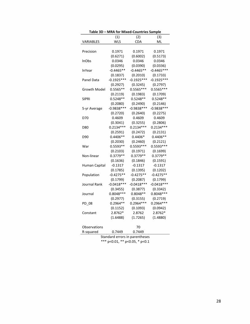
increases significantly which in turn affects growth negatively (military burden). The nonlinear effect of

ME is generally insignificant but is positive for the mixed-countries sample (Table 3D) in the WLS, CDA

and ML.

3.4.3. Publication Characteristics

First, we control for publication type, and examine whether journal articles tend to report different

estimates in comparison to working papers. Controlling for publication type makes it possible to

determine whether there is a predisposition to publish studies with statistically significant results,

congruent with theory to justify model selection. Thus, we include a dummy for journal articles in our

MRA, and leave out working papers as base. Overall, our results suggest that the effect of ME on growth

is more adverse for journal publications, and this is consistent across all sample, estimation and

specification types. In addition, we examine if the ME-G effect reported by primary studies varies with

the publication outlet used. Therefore, we control for high-ranked journals to determine if publication

outlet used affects reported effect sizes.8 For the entire sample (Table 3A), our results suggest that the

publication outlet used does not affect the ME-G effect. However, when we consider the samples of less

developed and developed countries, we find that high-ranked journals tend to report more negatively

on the ME-G relationship.

Next, we control for publication year. Controlling for publication year is necessary to verify if

reported effect sizes on the ME-G relationship change overtime as more studies emerge to challenge

the status quo with newer econometric techniques and richer datasets. Also, given that A-L consist only

32 studies out of 42 studies included in our study, we include a dummy variable to capture newer

studies which have not been included in their study. This would enable us to determine the effects of

newer studies on the ME-G relationship and also to examine if the inclusion of these new studies

contributes to our finding that shows a negative effect of ME on growth. In general, consistent with our

expectations, we find that studies not included in the meta-analysis of A-L (PD_08) tend to report

negatively on the effects of ME on growth. We also include dummies for studies that were published in

the 1970s and 80s (PD7_80), and also in 1990s (PD90) in our MRA. We use other studies which do not

fall in any of the three categories as the base. In general, our results indicate that the period of

8 The Australian Business Dean’s Council (ABDC) and the Australian Research Council (ARC) present classifications for journal

quality. Journals are ranked in descending order of quality as A*, A, B and C. Thus, we introduce a dummy for A* and A ranked

journals (high quality) in our MRA, and use other ranks as base.

15

publication presents variations in the reported estimates in that more recent studies (PD_08, PD90)

report negatively on the ME-G nexus.

Turning to the net effect of ME on growth after controlling for all relevant moderator variables,

we find that the coefficient of precision ( ⁄ ) across all estimations of the specific model is negative

and significant. Specifically, using the ML (Table 3A column 6) as our preferred estimation type, we find

that the coefficient of precision is -0.067. This is the measure of genuine empirical effect which takes

into account the selection bias and moderator variables. Based on Cohen’s guidelines, we conclude that

this effect is weak and of no practical significance. With regard to developed countries, the preferred ML

model (Table 3C column 3) shows that the coefficient of precision is 0.3020. This suggests that for

developed countries, the effect of ME on growth is positive. This result is quite robust across all

estimation types. For LDCs, CDA model (Table 3B column 4) indicates that the coefficient of precision is -

0.3510. This supports the hypothesis that ME is detrimental to growth in LDCs. Lastly, the results from

the mixed-countries sample mainly indicate that the coefficient of precision is insignificant.

4. Discussions and Conclusion

Based on 243 estimates drawn from 42 primary studies, we conduct a meta-analysis that examines the

following five hypotheses: (H1) Military expenditure (ME) as a proportion of GDP reduces growth, (H2)

ME as a proportion of GDP reduces growth in less developed countries (LDCs), (H3) ME as a proportion

of GDP increases growth, (H4) The effect of ME as a proportion of GDP on growth is non-linear, and (H5)

ME as a proportion of GDP increases growth in developed countries. The following major conclusions

emerge.

Using only the sample of 32 studies included in A-L, that is Alptekin and Levine (2012), we

confirm their results. However, with the addition of newer studies, mostly with newer datasets, their

general conclusion on the military expenditure-growth (ME-G) relationship, which indicates a positive

association, is no longer valid. The new conclusion (negative effect of ME on growth) could be as a result

of the increasing levels of ME recorded over time. Data shows that global ME has consistently increased

since 1998 except for a slight decline (about 0.5%) in 2011. This is also consistent with MRA results,

where we find that studies that include data from the 2000s report stronger negative effects of ME on

growth. Another possible reason for a negative effect of ME on growth is government corruption.

Mauro (1998) finds that corruption may induce more government spending on ME.

The results from fixed effects weighted averages, bivariate precision effect and funnel assymetry

tests (PET/FAT), and multivariate meta-regression analysis (MRA) all indicate that the ME-G effect is

16

negative and is estimated to be between -0.0401 and -0.0790 depending on whether publication

selection bias and/or moderator variables have been controlled for. Based on these results, it is obvious

that (H1) is supported but (H3) is rejected. Although negative, these results are practically negligible

according to Cohen’s guidelines. However, based on the guidelines recently introduced by Doucouliagos

(2011), this effect is not trivial. Doucouliagos (2011) indicates that the application of Cohen’s guidelines

to partial correlation coefficients understates the economic significance of empirical effect.

Our results also support (H2), that is ME is detrimental to growth in LDCs. This is inconsistent

with the findings presented by A-L. Additionally, by considering the coefficient of the precision for LDCs

only, both MRA (Table 3B column 4) and PET/FAT results (Table 2A panel 3) show a negative ME-G

effect. Thus, quite robustly, we can conclude that ME is detrimental to growth in LDCs.

The negative military effect on growth in LDCs may be due to the following reasons. LDCs in

general have lower government quality and more corrupt governments than developed countries (see

e.g., La Porta at al., 1999). Rent-seeking in the military sector increases the cost of military activities and

together with inefficient operations and high regulatory costs, ME tends to reduce growth in LDCs.

Moreover, raising taxes in LDCs may be difficult and thus, higher ME may be financed by higher

seigniorage which could lead to higher inflation and thus, lower savings.

LDCs also tend to suffer from political tensions, security threats or economic constraints.

Examples of political tensions in LDCs are interstate tensions in the Middle-East, Eastern Europe, South

Asia, the East China Sea and the South China Sea. Examples of security threats coming from intrastate

conflicts in LDCs include insurgencies, terrorism and other civil conflicts.9 It is a widely held view that

political tensions and associated high levels of ME tend to retard growth.

The opportunity cost of ME may be sufficiently large in insecure regions where as a net effect,

high ME may aggravate distortions, reduce the efficiency of resource allocation, and crowd out

productive activities such as R&D, and investment in physical and human capital in these regions.10

Insecure regions tend to devote a disproportionate share of the scarce resources to military which may

adversely affect the composition of government expenditure.11 ME may also worsen the balance of

9 According to Dahal et al. (2003), all nine countries in South Asia have experienced internal conflict in the last two decades.

Moreover, more of the conflicts have been in the poorer regions of those countries than elsewhere since 2001 (Iyer, 2009).

10 Knight et al. (1996) find that ME reduces growth through crowding-out and distortion effects.

11 LDCs such as Saudi Arabia and Russia have increased their ME as a proportion of GDP from 8.1% to 9.3% and from 3.5% to

4.1%, respectively, between 2004 and 2013 (IMF, 2013). Devarajan et al. (1996) show that the change in the composition of

government spending affects a country’s economic growth.

17

payment for LDCs because most of these countries import military armaments from developed

countries (see, e.g., Knight et al., 1996).

MRA and PET/FAT results for the developed-countries sample consistently lend support to the

finding of A-L which suggests that (H3) is supported for developed countries. In essence, (H5) is also

supported. For our prefered specification, PET/FAT and MRA results show that the coefficient of

precision is 0.1564 and 0.3020, respectively. One explanation offered by A-L which supports (H5) is that

relative to LDCs, most developed countries record low levels of ME and thus, the benefits outweigh the

opportunity cost of ME. However, based on the recent data from World Bank (World Development

Indicators), ME as a share of GDP remains lower for LDCs relative to develop countries. Thus, there may

be other reasons why ME promotes growth in developed countries.

One possible explanation for (H5) is that developed countries tend to be arms exporters (see the

information from the Stockholm International Peace Research Institute, for instance), while LDCs tend to

be arms importers. Countries that increase miliatary expenditure tend to face less balance of payment

difficulties when they increase military exports at the same time. Arms exporters are more likely to

enjoy the “Keynesian effect” whereby increases in ME generates effective demand, leading to growth.

Furthermore, considering the high levels of military related R&D in developed countries, the civilian

sector is likely to experience positive externalities. It is also possible that ME in developed countries

tend to provide security and respect internationally, while ME in LDCs are more likely to increase their

dependency on aid and increase political conflict. Additionally, our results do not support (H4) as the

dummy for studies that formulate a nonlinear ME-G relationship is insignificant.

With regard to systematic heterogeneity in the ME-G literature, we find that differences in

primary studies that contribute to variations in the reported effect sizes include data period, data type,

data source, period of data averaging and control variables included in econometric specifications.

These results confirm those presented by A-L, and also conclusions drawn by earlier surveys such as

Dunne (1996).

Overall, our findings show that meta-analysis is effective in sythesizing evidence when the

evidence base is broad and is accompanied by a high level of heterogeneity. This study has derived

verifiable conclusions about the effects of miliatary expenditure on growth, and has accounted for

about 54% to 74% of the variations in the evidence base. We identify a number of shortcomings which

are relevant to guide future research. First, given that our result on the nonlinear effect of ME

contradicts that of A-L, it would be useful to futher explore this relationship in future research.

Particularly, as our results suggest that higher levels of ME are associaited with lower economic

18

performance, future research can focus on determining a threshold beyond which further increments in

ME become detrimental to growth. Additionally, given the hypothesized relationship between

corruption and ME (see, e.g., Mauro, 1998), it would be worthwhile for future studies to explore this

relationship more thoroughly. As it stands, only few studies control for corruption in their ME-G models.

In conclusion, ME is an important aspect of fiscal policy-growth relationship and has received

considerable attention from researchers and policy analysts. Our findings offer a useful policy

implication on whether ME is the component of government expenditure to adjust in order to promote

growth in a context of limited economic resources and fiscal constraints.

19

References

Aizenman, J. and R. Glick. 2006. Military expenditure, threats, and growth. The Journal of International Trade & Economic Development 15, no 2: 129-29.

Alptekin, A. and P. Levine. 2012. Military expenditure and economic growth: A meta-analysis. European Journal of Political Economy 28, no 4: 636-50.

Antonakis, N. 1997. Military expenditure and economic growth in greece, 1960-90. Journal of Peace Research 34, no 1: 89-100.

Barro, R.J. 1990. Government spending in a simple model of endogenous growth. Journal of Political Economy 98, no 5: S103-S25.

Batchelor, P., J.P. Dunne and D.S. Saal. 2000. Military spending and economic growth in south africa. Defence and peace economics 11, no 4: 553-71.

Benoit, E. 1973. Defense and economic growth in developing countries. Lexington: Lexington Books. Benoit, E. 1978. Growth and defense in developing countries. Economic Development and Cultural

Change 26, no 2: 271-80. Biswas, B. 1993. Defense spending and economic growth in developing countries. Boulder, CO: West

view Press. Biswas, B. and R. Ram. 1986. Military expenditures and economic growth in less developed countries: An

augmented model and further evidence. Economic Development and Cultural Change 34, no 2: 361-72.

Blomberg, S.B. 1996. Growth, political instability and the defence burden. Economica 63, no 252: 649-72.

Bose, N., M.E. Haque and D.R. Osborn. 2007. Public expenditure and economic growth: A disaggregated analysis for developing countries. Manchester School 75, no 5: 533-56.

Brumm, H.J. 1997. Military spending, government disarray, and economic growth: A cross-country empirical analysis. Journal of Macroeconomics 19, no 4: 827-38.

Cappelen, Å., N.P. Gleditsch and O. Bjerkholt. 1984. Military spending and economic growth in the oecd countries. Journal of Peace Research 21, no 4: 361-73.

Chan, S. 1987. Military expenditures and economic performance. In World military expenditures and arms transfers: US Arms Control and Disarmament Agency, US Govt Printing Office.

Chan, S. 1988. Defense burden and economic growth: Unraveling the taiwanese enigma. The American Political Science Review 82, no 3: 913-20.

Chen, P., C. Lee and Y. Chiu. 2014. The nexus between defense expenditure and economic growth: New global evidence. Economic Modelling 36: 474-74.

Cohen, J. 1988. Statistical power analysis for the behavioural sciences Hillsdale, NJ. Cooray, A. 2009. Government expenditure, governance and economic growth. Comparative Economic

Studies 51, no 3: 401-18. D'agostino, G., J.P. Dunne and L. Pieroni. 2013. Military expenditure, endogeneity and economic growth.

MPRA Working Paper No. 45640. D’agostino, G., J.P. Dunne and L. Pieroni. 2010. Assessing the effects of military expenditure on growth

In Oxford Handbook of the Economics of Peace and Conflict. Oxford University Press. Dahal, S.H., H. Gazdar, S.I. Keethaponcalan and P. Murthy. 2003. Internal conflict and regional security in

south asia. United Nations Institute for Disarmament Research, Geneva. De Dominicis, L., R. Florax and H. Groot. 2008. A meta-analysis on the relationship between income

inequality and economic growth. Scottish Journal of Political Economy 55, no 5: 654-82. Deger, S. 1986. Economic development and defense expenditure. Economic Development and Cultural

Change 35, no 1: 179-96.

20

Deger, S. and S. Sen. 1983. Military expenditure, spin-off and economic development. Journal of Development Economics 13, no 1–2: 67-83.

Deger, S. and R. Smith. 1983. Military expenditure and growth in less developed countries. The Journal of Conflict Resolution 27, no 2: 335-53.

Degrasse, R. 1983. Military expansion economic decline: The impact of military spending on u.S. Economic performance. . Armonk, NY: M. E. Sharpe.

Derouen, K. 2000. The guns-growth relationship in israel. Journal of Peace Research 37, no 1: 69-83. Derouen, K.R. 1994. Defense spending and economic growth in latin america: The externalities effects.

International Interactions 19, no 3: 193-212. Doucouliagos, H. 2011. How large is large? Preliminary and relative guidelines for interpreting partial

correlations in economics. Deakin University, School of Accounting, Economics and Finance Working Paper Series, no 5.

Dunne, J.P. 1996. Economic effects of military spending in LDCs: A survey. In The peace dividend (contributions to economic analysis series), eds Gleditsch, NP, Cappelen, A, Bjerkholt, O, Smith, R and Dunne, P, 439–64. North Holland, Amsterdam.

Dunne, J.P. and N.L. Mohammed. 1995. Military spending in sub-saharan africa: Some evidence for 1967-85. Journal of Peace Research 32, no 3: 331-43.

Dunne, J.P., R.P. Smith and D. Willenbockel. 2005. Models of military expenditure and growth: A critical review. Defence and peace economics 16, no 6: 449-61.

Dunne, J.P. and N. Tian. 2013. Military spending conflict economic growth africa. SIPRI Working Paper. Dunne, J.P. and M. Uye. 2009. Military spending and development. . In The global arms trade, ed. Tan, A.

London: Europa/Routledge. Dunne, P., E. Nikolaidou and D. Vougas. 2001. Defence spending and economic growth: A causal analysis

for greece and turkey*. Defence and peace economics 12, no 1: 5-26. Egger, M., G. Smith, M. Schnieder and C. Minder. 1997. Bias in meta-analysis detected by a simple,

graphical test. British Medical Journal 315: 629–34. Faini, R., P. Annez and L. Taylor. 1984. Defense spending, economic structure, and growth: Evidence

among countries and over time. Economic Development and Cultural Change 32, no 3: 487-98. Frederiksen, P.C. and R.E. Looney. 1983. Defense expenditures and economic growth in developing

countries. Armed Forces and Society 9: 633-45. Galvin, H. 2003. The impact of defence spending on the economic growth of developing countries: A

cross-section study. Defence and peace economics 14, no 1: 51-59. Goldstein, H. 1995. Multilevel statistical models 2nd ed. London: Edward Arnold. Grobar, L.M. and R.C. Porter. 1989. Benoit revisited: Defense spending and economic growth in LDCs.

Journal of Conflict Resolution 33, no 2: 318-45. Gyimah-Brempong, K. 1989. Defense spending and economic growth in subsaharan africa: An

econometric investigation. Journal of Peace Research 26, no 1: 79-90. Henmi, M. and J.B. Copas. 2010. Confidence intervals for random effects meta-analysis and robustness

to publication bias. Stat Med 29, no 29: 2969-83. Heo, U. 1999. Defense spending and economic growth in south korea: The indirect link. Journal of Peace

Research 36, no 6: 699-708. Heo, U. and K. Derouen. 1998. Military expenditures, technological change, and economic growth in the

east asian nics. The Journal of Politics 60, no 3: 830-46. Hou, N. and B. Chen. 2013. Military expenditure and economic growth in developing countries: Evidence

from system gmm estimates. Defence and peace economics 24, no 3: 183-83. International Monetary Fund, 2013. World economic outlook database. Iyer, L. 2009. The bloody millennium: Internal conflict in south asia. Harvard Business School, Working

Paper 09-086, Cambridge, MA.

21

Kalaitzidakis, P. and V. Tzouvelekas. 2011. Military spending and the growth-maximizing allocation of public capital: A cross-country empirical analysis. Economic Inquiry 49, no 4: 1029-41.

Kelly, T. 1997. Public expenditures and growth. Journal of Development Studies 34, no 1: 60-84. Kennedy, G. 1983. Defense economics. . London: Duckworth. Kinsella, D. 1990. Defence spending and economic performance in the united states: A causal analysis.

Defence Economics 1, no 4: 295-309. Knight, M., N. Loayza and D. Villanueva. 1996. The peace dividend: Military spending cuts and economic

growth. Staff Papers - International Monetary Fund 43, no 1: 1-37. Kollias, C., N. Mylonidis and S.-M. Paleologou. 2007. A panel data analysis of the nexus between defence

spending and growth in the european union. Defence and peace economics 18, no 1: 75-75. La Porta, R., F. Lopez-De-Silanes, A. Shleifer and R. Vishny. 1999. The quality of government. Journal of

Law, Economics and Organization 15, no 1: 222-79. Landau, D. 1986. Government and economic growth in the less developed countries: An empirical study

for 1960-1980. Economic Development and Cultural Change 35, no 1: 35-75. Landau, D. 1994. The impact of military expenditures on economic growth in the less developed

countries. Defence and peace economics 5, no 3: 205-20. Landau, D. 1996. Is one of the ‘peace dividends’ negative? Military expenditure and economic growth in

the wealthy oecd countries. The Quarterly Review of Economics and Finance 36, no 2: 183-95. Lebovic, J.H. and A. Ishaq. 1987. Military burden, security needs, and economic growth in the middle

east. The Journal of Conflict Resolution 31, no 1: 106-38. Levine, R. and D. Renelt. 1992. A sensitivity analysis of cross-country growth regressions. The American

Economic Review 82, no 4: 942-63. Lim, D. 1983. Another look at growth and defense in less developed countries. Economic Development

and Cultural Change 31, no 2: 377-84. Lipow, J. and C.M. Antinori. 1995. External security threats, defense expenditures, and the economic

growth of less-developed countries. Journal of Policy Modeling 17, no 6: 579-95. Looney, R. and R.M. Mcnab. 2008. Can economic liberalization and improved governance alter the

defense–growth trade-off? Review of Financial Economics 17, no 3: 172-82. Looney, R.E. 1989. Impact of arms production on income distribution and growth in the third world.

Economic Development and Cultural Change 38, no 1: 145-53. Mauro, P. 1998. Corruption and the composition of government expenditure. Journal of Public

Economics 69, no 2: 263-79. Miller, S.M. and F.S. Russek. 1997. Fiscal structures and economic growth: International evidence.

Economic Inquiry 35, no 3: 603-13. Mintz, A. and C. Huang. 1990. Defense expenditures, economic growth, and the "peace dividend". The

American Political Science Review 84, no 4: 1283-93. Mintz, A. and C. Huang. 1991. Guns versus butter: The indirect link. American Journal of Political Science

35, no 3: 738-57. Mintz, A. and R.T. Stevenson. 1995. Defense expenditures, economic growth, and the "peace dividend".

The Journal of Conflict Resolution 39, no 2: 283-83. Mueller, M.J. and H.S. Atesoglu. 1993. Defense spending, technological change, and economic growth in

the united states. Defence Economics 4, no 3: 259-69. Myo, K. 2013. Military expenditures and economic growth in asia. SIPRI Working Paper. Na, H. and C. Bo. 2013. Military expenditure and economic growth in south asia. Contributions to

Conflict Management, Peace Economics and Development, Volume 20: 213-23. Payne, J.E. and K.L. Ross. 1992. Defense spending and the macroeconomy. Defence Economics 3, no 2:

161-68.

22

Pieroni, L. 2009a. Does defence expenditure affect private consumption? Evidence from the united states. Economic Modelling 26, no 6: 1300-09.

Pieroni, L. 2009b. Military expenditure and economic growth. Defence and peace economics 20, no 4: 327-27.

Ram, R. 2003. Defence expenditure and economic growth: Evidence from recent cross-country panel data. In The elgar companion to public economics: Empirical public economics, eds Attiat, O and Cebula, R, 166–98: Edward Elgar.

Smaldone, J.P. 2006. African military spending: Defence versus development? African Security Review 15, no 4: 18–32.

Smith, R. 1992. Measuring the effects of military spending: Cross-sections or time-series? Paper presented at the ICEIS, in The Hague, the Netherlands.

Smith, R.P. 1980. Military expenditure and investment in oecd countries, 1954–1973. Journal of Comparative Economics 4, no 1: 19-32.

Stanley, T. 2008. Meta-regression methods for detecting and estimating empirical effects in the presence of publication selection. Oxford Bulletin of Economics and Statistics 70, no 2: 103-27.

Stanley, T. and H. Doucouliagos. 2007. Identifying and correcting publication selection bias in the efficiency-wage literature: Heckman meta-regression. In Economics Series 2007, 11. Deakin University.

Stanley, T. and H. Doucouliagos. 2012. Meta-regression analysis in economics and business. New York: Routledge.

Stanley, T.D. and H. Doucouliagos. 2014. Meta-regression approximations to reduce publication selection bias. Research Synthesis Methods 5, no 1: 60-78.

Stanley, T.D., H. Doucouliagos, M. Giles, J.H. Heckemeyer, R.J. Johnston, P. Laroche, J.P. Nelson, M. Paldam, J. Poot, G. Pugh, R.S. Rosenberger and K. Rost. 2013. Meta-analysis of economics research reporting guidelines. Journal of Economic Surveys 27, no 2: 390-94.

Stroup, M. and J. Heckelman. 2001. Size of the military sector and economic growth: A panel data analysis of africa and latin america. Journal of Applied Economics 4, no 2: 329-60.

Ugur, M. 2013. Corruption's direct effects on per-capita income growth: A meta-analysis. Journal of Economic Surveys.

Ward, M., A. Cochran, D. Davis, M. Penubarti and S. Rajmaira. 1992. Economic growth, investment, and military spending in india, 1950-88. In Defense, welfare, and growth, eds Chan, S and Mintz, A. London Routledge.

Ward, M.D. and D.R. Davis. 1992. Sizing up the peace dividend: Economic growth and military spending in the united states, 1948-1996. The American Political Science Review 86, no 3: 748-55.

Weede, E. 1983. Military participation ratios, human capital formation, and economic growth: A cross-mational analysis. J. of Political and Military Sociology 11: 11-19.

Yakovlev, P. 2007. Arms trade, military spending, and economic growth. Defence and peace economics 18, no 4: 317-17.

23

Table 1 (Overview of Evidence Base per Study - Simple & Fixed Effect Weighted Means)

Paper No. of

Estimates

Simple Mean

Weighted Mean

Significance

Confidence Interval

Aizenman and Glick (2006) 9 -0.1451 -0.1667 Yes (-0.2998, -0.0335)

Antonakis (1997) 2 -0.4592 -0.4594 Yes (-0.6228, -0.2960)

Benoit (1978) 3 0.3676 0.3851 No (-0.0355, 0.8057)

Biswas and Ram (1986) 6 0.1323 0.1949 Yes (0.0620, 0.3278)

Blomberg (1996) 1 -0.0419 -0.0419

Bose et al. (2007) 4 0.2509 0.2690 Yes (0.0528, 0.4852)

Brumm (1997) 2 0.3056 0.3170 No (-1.2011, 1.8351)

Cappelen et al. (1984) 8 0.0325 0.0276 No (-0.2427, 0.2978)

Chan (1988) 3 0.0919 0.0926 No (-0.1219, 0.3070)

Cooray (2009) 5 0.0388 0.0388 Yes (0.0016, 0.0759)

Deger (1986) 5 0.3275 0.3279 Yes (0.2960, 0.3599)

Deger and Sen (1983) 1 0.1462 0.1462

Deger and Smith (1983) 5 0.0089 0.0691 No (-0.2649, 0.4032)

DeRouen (2000) 1 0.1969 0.1969

Dunne and Mohammed (1995) 3 0.0295 0.0306 No (-0.3118, 0.2506)

Dunne and Tian (2013) 27 -0.1188 -0.1183 Yes (-0.1278, -0.1087)

Faini et al. (1984) 1 0.0601 0.0601

Galvin (2003) 9 -0.1412 -0.1438 Yes (-0.2366, -0.0511)

Grobar and Porter (1989) 5 0.2160 0.2517 No (-0.0692, 0.5727)

Gyimah-Brempong (1989) 2 0.0580 0.0581 No (-0.2219, 0.3380)

Heo and DeRouen (1998) 5 -0.1307 -0.1356 No (-0.3011, 0.0300)

Hou and Chen (2013) 6 -0.0824 -0.0829 Yes (-0.1510, -0.0148)

Kalaitzidakis and Tzouvelekas

(2011) 1 0.0720 0.0720

Kelly (1997) 8 0.0612 0.0610 No (-0.0240, 0.1460)

Knight et al. (1996) 4 -0.0538 -0.0550 No (-0.2409, 0.1310)

Kollias et al. (2007) 2 0.1557 0.1567 No (-0.5586, 0.8720)

Landau (1986) 12 -0.0587 -0.0003 No (-0.0425, 0.0419)

Landau (1994) 30 0.1894 0.1872 Yes (0.1567, 0.2177)

Landau (1996) 11 0.2849 0.2860 Yes (0.1429, 0.4291)

Lebovic and Ishaq (1987) 4 -0.0969 -0.1022 No (-0.3302, 0.1259)

Lim (1983) 9 -0.0478 0.0647 No (-0.2296, 0.3591)

Lipow and Antinori (1995) 2 0.2786 0.2991 No (-1.9812, 2.5793)

Looney (1989) 2 -0.0505 -0.2718 No (-5.7252, 5.1817)

Looney and McNab (2008) 4 -0.1071 -0.0893 No (-0.3917, 0.2131)

Miller and Russek (1997) 6 -0.1333 -0.1632 Yes (-0.2640, -0.0624)

Myo (2013) 5 0.1505 0.2058 Yes (0.1033, 0.3083)

Na and Bo (2013) 3 -0.4245 -0.4961 No (-1.1954, 0.2031)

Stroup and Heckelman (2001) 5 0.2416 0.2330 Yes (0.1239, 0.3421)

Yakovlev (2007) 10 -0.1459 -0.1563 Yes (-0.2210, -0.0916)

d’Agostino et al. (2010) 2 -0.2110 -0.2112 No (-0.4511, 0.0286)

d'Agostino et al. (2013) 10 -0.1365 -0.1349 Yes (-0.1665, -0.1034)

Total 243 0.0164 -0.0401

24

Table 2A – PET/FAT Results

Panel 1 Panel 2 Panel 3 Panel 4 Entire Dataset Developed Countries LDCs Mixed Countries

(1) (2) (3) (1) (2) (3) (1) (2) (3) (1) (2) (3) VARIABLES WLS CDA ML WLS CDA ML WLS CDA ML WLS CDA ML

Precision ( ) -0.1109*** -0.1109** -0.0264 0.1594** 0.1594** 0.1564** -0.0985*** -0.0985* 0.0323 -0.1283*** -0.1283*** -0.1328*** (0.0179) (0.0430) (0.0205) (0.0688) (0.0460) (0.0756) (0.0254) (0.0567) (0.0276) (0.0259) (0.0301) (0.0359) Bias ( ) 1.2108*** 1.2108** 0.3580 -0.1277 -0.1277 -0.5022 1.1474*** 1.1474 -0.3161 0.9379** 0.9379 1.8730*** (0.2595) (0.5319) (0.3735) (0.7157) (0.8823) (0.9508) (0.3398) (0.6754) (0.4828) (0.4593) (0.6430) (0.7198) Observations 243 26 147 70

Standard errors in parentheses *** p<0.01, ** p<0.05, * p<0.1

Table 2B – PEESE Results

(1) (2) (3) (4) (5) VARIABLES WLS CDA WLS WLS ML

Precision ( ) -0.0598*** -0.0598* -0.0428*** -0.1056*** -0.0917*** (0.0112) (0.0347) (0.0154) (0.0165) (0.0255) Standard Error ( ) 4.1462*** 4.1462* 3.2283** 7.2517** 15.0302*** (1.1999) (2.0961) (1.3872) (3.2662) (5.3717) Observations 243 147 70

Standard errors in parentheses *** p<0.01, ** p<0.05, * p<0.1

25

Table 3A – MRA for Entire Dataset

(1) (2) (3) (4) (5) (6) VARIABLES WLS WLS CDA CDA ML ML

Precision 0.1557 -0.0790*** 0.1557 -0.0790*** 0.1505 -0.0607* (0.2275) (0.0221) (0.1919) (0.0263) (0.2017) (0.0351) lnObs 0.0109 0.0109 0.0118 (0.0226) (0.0218) (0.0228) lnYear 0.0750 0.0750* 0.0481 (0.0620) (0.0425) (0.0536) Developed Countries 0.0320 0.0320 0.0277 (0.0484) (0.0485) (0.0501) Single Country -0.2902*** -0.2916*** -0.2902** -0.2916** -0.2714* -0.3019* (0.1093) (0.0681) (0.1274) (0.1164) (0.1542) (0.1554) Africa -0.0509** -0.0893*** -0.0509* -0.0893*** -0.0661** -0.0684*** (0.0207) (0.0179) (0.0277) (0.0204) (0.0262) (0.0231) Panel Data -0.0863 -0.0863 -0.0303 (0.1216) (0.0649) (0.0802) Growth Model -0.0880 -0.0880* -0.0864 (0.0702) (0.0485) (0.0647) SEM -0.0175 0.0515 -0.0175 0.0515 0.0276 0.0800* (0.0748) (0.0444) (0.0627) (0.0373) (0.0782) (0.0481) SIPRI 0.0260 0.1130*** 0.0260 0.1130*** 0.0417 0.0831** (0.0491) (0.0225) (0.0394) (0.0246) (0.0505) (0.0342) ACDA -0.0106 -0.0245 -0.0106 -0.0245 -0.0413 -0.0850* (0.0991) (0.0287) (0.0755) (0.0433) (0.0894) (0.0489) 5-yr Average -0.0782*** -0.0876*** -0.0782*** -0.0876*** -0.0736*** -0.0657** (0.0275) (0.0218) (0.0298) (0.0256) (0.0285) (0.0273) D50 0.1455 0.1956*** 0.1455** 0.1956*** 0.1833** 0.2484*** (0.0949) (0.0551) (0.0703) (0.0514) (0.0904) (0.0868) D60 -0.1070 -0.1070** -0.0325 (0.0783) (0.0518) (0.0631) D80 -0.0157 -0.0157 -0.0381 (0.1145) (0.0905) (0.1117) D90 0.1331*** 0.0816*** 0.1331*** 0.0816*** 0.1414*** 0.1179*** (0.0475) (0.0217) (0.0400) (0.0218) (0.0514) (0.0306) D00 -0.1198 -0.1198** -0.1229* (0.0823) (0.0531) (0.0659) War -0.1079* -0.1079** -0.0687 (0.0629) (0.0437) (0.0552) Non-Linear 0.0702 0.0702 0.0009 (0.1137) (0.0842) (0.1078) Investment -0.0974 -0.0974* -0.0092 (0.0775) (0.0537) (0.0615) Human Capital 0.0008 0.0008 -0.0202 (0.0874) (0.0585) (0.0704) Population -0.0838*** -0.1472*** -0.0838*** -0.1472*** -0.1626*** -0.1749*** (0.0246) (0.0161) (0.0293) (0.0180) (0.0440) (0.0314) Initial GDP 0.1731** 0.1323*** 0.1731*** 0.1323*** 0.1864*** 0.1137*** (0.0836) (0.0216) (0.0471) (0.0216) (0.0584) (0.0334) Journal Rank 0.1122 0.1122 0.0610 (0.1050) (0.0753) (0.0953) Journal -0.2367*** -0.2367*** -0.2586*** (0.0857) (0.0620) (0.0734) PD7_80 -0.1471 -0.1471 -0.0979

26

(0.1280) (0.0950) (0.1268) PD90 -0.1624 -0.1624* -0.0878 (0.1111) (0.0878) (0.1095) PD_08 -0.1181* -0.1181** -0.1033 (0.0626) (0.0562) (0.0745) Constant 0.0506 0.0233 0.0506 0.0233 -0.0018 -0.1889 (0.5191) (0.2451) (0.5487) (0.2411) (0.5707) (0.3293) Observations 243 R-squared 0.6240 0.5357 0.6240 0.5357

Robust standard errors in parentheses *** p<0.01, ** p<0.05, * p<0.1

Table 3B – MRA for LDCs

(1) (2) (3) (4) (5) (6) VARIABLES WLS WLS CDA CDA ML ML

Precision -0.0482 -0.3510 -0.0482 -0.3510* -0.0482 -0.0929 (0.3404) (0.2629) (0.2133) (0.1866) (0.1982) (0.2093) lnObs 0.0612* 0.0793** 0.0612** 0.0793*** 0.0612** 0.0492* (0.0335) (0.0358) (0.0285) (0.0259) (0.0265) (0.0284) lnYear 0.0291 0.0803*** 0.0291 0.0803*** 0.0291 0.0718** (0.0597) (0.0187) (0.0477) (0.0240) (0.0443) (0.0339) Single Country 0.0241 0.0241 0.0241 (0.1435) (0.1820) (0.1692) Africa 0.0135 0.0135 0.0135 (0.0296) (0.0361) (0.0336) Panel Data 0.0674 0.0674 0.0674 (0.0941) (0.0852) (0.0792) SEM 0.1713*** 0.1983*** 0.1713*** 0.1983*** 0.1713*** 0.2026*** (0.0496) (0.0479) (0.0528) (0.0445) (0.0491) (0.0578) SIPRI -0.0348 -0.0348 -0.0348 (0.1209) (0.0571) (0.0531) 5-yr Average -0.0601*** -0.0794*** -0.0601* -0.0794*** -0.0601** -0.0622** (0.0180) (0.0205) (0.0321) (0.0286) (0.0298) (0.0280) D50 0.2414 0.2864*** 0.2414* 0.2864*** 0.2414* 0.3064*** (0.2692) (0.1005) (0.1373) (0.0839) (0.1276) (0.1180) D80 -0.0333 -0.0333 -0.0333 (0.1321) (0.0840) (0.0781) D90 0.1836 0.1836** 0.1836** (0.2679) (0.0922) (0.0857) War -0.3097*** -0.1722*** -0.3097*** -0.1722*** -0.3097*** -0.1914*** (0.1135) (0.0339) (0.0662) (0.0305) (0.0615) (0.0451) Investment -0.1211 -0.1211** -0.1211** (0.0849) (0.0602) (0.0560) Population -0.0274 -0.0658*** -0.0274 -0.0658** -0.0274 -0.0962** (0.0212) (0.0183) (0.0311) (0.0260) (0.0289) (0.0427) Journal Rank -0.3446 -0.2754*** -0.3446** -0.2754*** -0.3446*** -0.2552*** (0.2226) (0.0483) (0.1392) (0.0557) (0.1294) (0.0784) PD7_80 0.1660 0.1660 0.1660 (0.3033) (0.1730) (0.1608) PD90 -0.2229 -0.2086*** -0.2229 -0.2086*** -0.2229 -0.2392*** (0.1426) (0.0514) (0.1483) (0.0578) (0.1379) (0.0797) PD_08 -0.4496** -0.3373*** -0.4496*** -0.3373*** -0.4496*** -0.3355***

27

(0.1882) (0.0451) (0.1321) (0.0590) (0.1228) (0.0829) Constant 0.1625 0.8270 0.1625 0.8270 0.1625 -0.0316 (0.7266) (0.7128) (0.6171) (0.5729) (0.5735) (0.6551) Observations 147 R-squared 0.6479 0.6029 0.6479 0.6029

Standard errors in parentheses *** p<0.01, ** p<0.05, * p<0.1

Table 3C – MRA for Developed-Countries Sample

(1) (2) (3) VARIABLES WLS CDA ML

Precision 0.3020** 0.3020* 0.3020** (0.1262) (0.1734) (0.1442) Single Country 0.4114*** 0.4114 0.4114* (0.0992) (0.2919) (0.2428) Growth Model -0.2283** -0.2283 -0.2283** (0.0993) (0.1371) (0.1141) SIPRI -0.1419 -0.1419 -0.1419 (0.1037) (0.1270) (0.1057) War -0.7963*** -0.7963** -0.7963*** (0.0985) (0.3438) (0.2860) Investment 0.4850*** 0.4850** 0.4850*** (0.1189) (0.1933) (0.1608) Journal Rank -0.3527*** -0.3527 -0.3527* (0.0670) (0.2192) (0.1824) Constant -0.1286 -0.1286 -0.1286 (0.7947) (1.3123) (1.0919) Observations 26 R-squared 0.6543 0.6543

Standard errors in parentheses *** p<0.01, ** p<0.05, * p<0.1

28

Table 3D – MRA for Mixed-Countries Sample

(1) (2) (3) VARIABLES WLS CDA ML

Precision 0.1971 0.1971 0.1971 (0.6271) (0.6002) (0.5173) lnObs 0.0346 0.0346 0.0346 (0.0295) (0.0390) (0.0336) lnYear -0.4465** -0.4465** -0.4465*** (0.1837) (0.2010) (0.1733) Panel Data -0.1925*** -0.1925*** -0.1925*** (0.2927) (0.3245) (0.2797) Growth Model 0.5565** 0.5565*** 0.5565*** (0.2119) (0.1983) (0.1709) SIPRI 0.5248** 0.5248** 0.5248** (0.2080) (0.2490) (0.2146) 5-yr Average -0.9838*** -0.9838*** -0.9838*** (0.2720) (0.2640) (0.2275) D70 0.4609 0.4609 0.4609 (0.3041) (0.3255) (0.2806) D80 0.2134*** 0.2134*** 0.2134*** (0.2591) (0.2472) (0.2131) D90 0.4406** 0.4406* 0.4406** (0.2030) (0.2460) (0.2121) War 0.5593** 0.5593*** 0.5593*** (0.2103) (0.1971) (0.1699) Non-linear 0.3779** 0.3779** 0.3779** (0.1636) (0.1846) (0.1591) Human Capital -0.1317 -0.1317 -0.1317 (0.1785) (0.1395) (0.1202) Population -0.4275** -0.4275** -0.4275** (0.1799) (0.2087) (0.1799) Journal Rank -0.0418*** -0.0418*** -0.0418*** (0.3455) (0.3877) (0.3342) Journal 0.8048*** 0.8048** 0.8048*** (0.2977) (0.3155) (0.2719) PD_08 0.2964** 0.2964*** 0.2964*** (0.1152) (0.1093) (0.0942) Constant 2.8762* 2.8762 2.8762* (1.6488) (1.7265) (1.4880) Observations 70 R-squared 0.7449 0.7449

Standard errors in parentheses *** p<0.01, ** p<0.05, * p<0.1

29

Figures 1 - 4 Entire Dataset (1) Developed Countries (2)

LDCs (3)

Mixed Countries (4)

01

02

03

04

05

0

pre

cis

ion2

-1 -.5 0 .5partial_r

51

01

52

02

5

pre

cis

ion2

-.5 0 .5partial_r

01

02

03

04

0

pre

cis

ion2

-1 -.5 0 .5partial_r

01

02

03

04

05

0

pre

cis

ion2

-.4 -.2 0 .2 .4partial_r

30

Appendix Table A1 (MRA Variables)

Variables Definition

lnObs Natural logarithm of number of observation in PS lnYear Natural logarithm of number of years in PS Developed Countries 1 if the PS data is for developed countries, otherwise 0 Single Country Study 1 if a single time series analysis of a country is done, otherwise 0 Africa 1 if only African countries data is used, otherwise 0 Panel Data 1 if panel data is used in PS, otherwise 0. Growth Model 1 if the model is based on growth model, otherwise 0. SEM 1 if estimation method is simultaneous equations approach, otherwise 0 SIPRI 1 if data used in PS comes from SIPRI, otherwise 0 ACDA 1 if data used in PS comes from ACDA, otherwise 0 5-yr Average 1 if PS uses 5-year data averaging, otherwise 0 D50 1 if PS includes data from 1950s, otherwise 0 D60 1 if PS includes data from 1960s, otherwise 0 D80 1 if PS includes data from 1980s, otherwise 0 D90 1 if PS includes data from 1990s, otherwise 0 D00 1 if PS includes data from 2000s, otherwise 0 War 1 if PS control for instability or war, otherwise 0 Non-Linear 1 if PS control for non-linear, otherwise 0 Investment 1 if PS control for investment, otherwise 0 Human Capital 1 if PS control for human capital, otherwise 0 Population 1 if PS control for population, otherwise 0 Initial GDP 1 if PS control for initial GDP, otherwise 0 Journal Rank 1 if PS is published in high-ranked journal, otherwise 0 Journal 1 if PS is a journal paper, otherwise 0 PD7_80 1 if PS is published in the 1970s or 80s, otherwise 0 PD90 1 if PS is published in the 1990s, otherwise 0 PD_08 1 if PS is not included in Alptekin and Levine (2012), otherwise 0

*All variables are divided by * PS refers to primary study