Embed Size (px)
Citation preview

1
Department of Economics School of Social Sciences
The demand for long distance travel in Great Britain: some new evidence
Dimitrios Asteriou1, John Cubbin1, Ian Jones1, Paul Metcalfe2, Daniel Paredes2 and Jan Peter van der Veer2
1. Department of Economics, City University. 2. NERA Economic Consulting, 15 Stratford Place, London, W1C 1BE.
Address for correspondence: Ian Jones, Centre for the Study of Regulation and Competition, Department of Economics, City University, Northampton Square, London EC1V 0HB.
Department of Economics Discussion Paper Series
No. 05/01

2
Introduction
This paper presents estimates of the elasticities of demand for longer distance passenger rail travel in Great Britain, and is based on research undertaken for the UK Strategic Rail Authority (SRA). The background to the project is that there is a lack of clarity regarding the timescale over which the current elasticities in the Passenger Demand Forecasting Handbook (PDFH) 1 are intended to apply. For certain uses of the Handbook, such as investment appraisal and long-term planning, it would be desirable to have long-term elasticities. In other contexts, notably short term business and financial planning, rail business managers require advice on the response of demand to price changes in the short run, defined as a period of about a year after the fare change has occurred. The PDFH indicates that the elasticity values it recommends are intended to represent the change in demand that occurs within a year of a change in fares. This definition implies that demand effects occurring in the longer term are not addressed. It also implies that the elasticities do not offer guidance on the short run response of demand within the year.
In the present project, we have undertaken extensive econometric analysis on large data sets which has enabled us not only to derive long-term fare elasticities, but also to examine the dynamics of the demand response to changes in price and other factors. Although our research has investigated the demand characteristics of both short (commuter) and long distance journeys, the present paper focuses on the results obtained for longer distance journeys between the London Travelcard Area (the London TCA) and the rest of Great Britain, and between major urban centres other than London.2 Flows of this kind have been the subject of extensive previous research and the results of the earlier research can be compared directly with those obtained in the present study.3
The data used in the study covered the period from April 1989 to March 2003. We were therefore able to examine not only the effects of variations in fares and economic activity, but also the impact of a major external shock that occurred as a result of the Hatfield accident in October 2000, which resulted in major disruptions and a consequent dramatic reduction in service quality across the entire rail network.
The paper is organised as follows.
• We begin by summarising the results of previous studies into long term elasticities for the relevant market segments;
• the following section discusses the data and the empirical methodology used in the research. We describe the general form of the model of rail demand we have applied;
1 Often referred to in the rail industry as the PDFH. The PDFH is a reference document intended to offer guidance to rail sector managers involved in operational and longer term planning activities.
2 Appendix 2 presents a full list of the rail flows examined in this study. 3 We hope to publish the results of our analysis of shorter distance journeys in a subsequent paper.

3
the data set used in the modelling work, including the issues of disaggregation by ticket type and by type of flow; the estimation issues we have addressed in the research; and the econometric framework;
• we then present the results of the estimations we have undertaken;
• we finish with some concluding remarks.
There are three appendices to the paper. Appendix 1 discusses the technical econometric issues of cointegration and of multicollinearity. Appendix 2 lists the flows and ticket type categories used in the analysis, and Appendix 3 gives detailed estimation results.
Survey of Previous Work
The Demand for Longer Distance Rail Travel
Three previous studies produced estimates of long-term demand elasticities for longer distance rail travel in Great Britain.4 These are:
• a study by Jones and Nichols (1983) on the demand for London-based inter-city rail travel;
• a study by Owen and Phillips (1987) on the characteristics of inter-city railway passenger demand; and
• a study by NERA (1999) undertaken as part of wider research into forecasting passenger rail demand.
Jones and Nichols (1983) estimated static demand functions for 17 London-based inter-city flows for the period from 1970 to 1976 using four-weekly ticket sale data similar to those used in the present study. The measure of demand used in the study was total ticket sales aggregated over all types of ticket, and the fare variable was the average revenue per ticket, defined as total revenue divided by total ticket sales in each four-weekly period. As well as estimating the elasticity of demand with respect to fares, Jones and Nichols also examined the effects on the demand for rail travel of variations in real GDP, cyclical economic activity, rail service levels, service levels on competing modes of transport, and seasonal factors. As shown in Table 1, the average long run fare elasticity for the sample of flows in the Jones and
4 In addition to these studies, the UK Department for Transport (DfT) has also reported the results of research carried out within the Department on the total demand for rail services and on the demand for non-commuter rail services for the period from 1978/79 to 1998/99. The DfT reports estimates of elasticities of demand for non-commuter rail travel of –1.1 with respect to average fares, 2.2 with respect to GDP, and –1.1 with respect to the level of car traffic. However, it is difficult to comment on these results because few details are given on either the data or the econometric methods used in the study.

4
Nichols study was –0.64. The authors found that whilst rail demand was sensitive to the level of cyclical economic activity, the elasticity of demand with respect to GDP was generally not significantly different from zero.
Owen and Phillips (1987) analysed the demand for rail travel on 20 London-based inter-city rail flows, using four-weekly ticket sale data for the period from 1973 to 1984 drawn from the same database used by Jones and Nichols. Partial adjustment models were estimated for total demand aggregated over all ticket types and for demand disaggregated into first and second class ticket sales. For the aggregate model, the fares variable was defined in the same way as in the Jones and Nichols study. For the disaggregated analysis, the fare was defined as the average revenue for tickets sold in each disaggregated ticket category. In the latter case, an additional fares variable was added so that both own and cross price elasticities could be estimated. As shown in Table 1, the average long-term aggregate fares elasticity estimated by Owen and Phillips was –1.08. Like Jones and Nichols, Owen and Phillips also studied the effects on the demand for rail travel of macroeconomic activity, rail service levels, service levels on other transport modes, and seasonal factors. In the case of GDP elasticities, nine out of their 20 estimates were not significantly different from zero. Similar problems affected their estimated time trends.
More recently, NERA (1999) undertook an econometric study of rail passenger demand on both London-based and non-London-based flows over the period 1989 – 99 for the Office of Passenger Rail Franchising (OPRAF). NERA’s econometric analysis, which used four-weekly ticket sale data similar to those used in the Jones and Nichols and Owen and Phillips studies, produced estimates of the elasticity of demand (aggregated across ticket types) with respect to fare (estimated as total revenue across all ticket types divided by total journeys) and other explanatory variables, including GDP, rail service levels, petrol prices and seasonal factors. Two estimation methods were used to derive elasticities:
• static panel data estimation; and
• dynamic flow-by-flow estimation, incorporating a lagged dependent variable, similar to the approach used by Owen and Phillips.
Approaches to combining the panel and dynamic approaches were also explored using the “Pooled Mean Group” method. As shown in Table 1, NERA’s estimate of the long run fares elasticity for London-based flows obtained from the dynamic estimation was –0.61, strikingly similar to the Jones and Nichols estimate, but significantly less than the Owen and Phillips estimate. For non-London based flows, NERA estimated a fares elasticity of –0.97 using the same dynamic estimation approach. In contrast to the two earlier studies, NERA’s results suggested that the demand for inter-city rail travel was significantly income elastic. The average GDP elasticity for London based flows was 1.56, and was 1.2 for non-London based flows.

5
Table 1 Previous Estimates of Long Run Fares Elasticities
Study Type of Flow Level of Aggregation
Period of estimation
Elasticity estimate
Jones and Nichols (1983)
London based Aggregated 1970.1-1976.13 -0.64
Owen and Philips (1987)
London based Aggregated 1973.1-1984.13 -1.08
NERA (1999) London based Aggregated 1989.1-1999.13 -0.61 Non-London
based Aggregated 1989.1-1999.13 -0.90
Other Studies
Dargay and Hanly (2002) examined the demand for local bus services in England, using annual data for the period from 1986 to 1996 on bus patronage, fares and other relevant factors influencing bus use. For England as a whole, the Dargay-Hanly results indicate that the fare elasticity is likely to be about –0.4 in the short run and –0.9 in the long run. Demand is more price sensitive at higher fare levels, with the elasticity value in the short/long-run ranging from 0.1/0.2 for the lowest fares to 0.8/1.4 for the highest fares. Demand was also found to be more price sensitive in the so-called Shire counties, where average elasticities were –0.49 in the short run and –0.66 in the long run, than in the more highly urbanised Metropolitan counties, where the average elasticities were –0.26 in the short run and –0.54 in the long run.
Dargay and Hanley found that the income elasticity of demand for local bus services was significantly negative, both in the Shire counties, where the estimated income elasticity of demand was –0.43 in the short term, and – 0.58 in the long term, and in the Metropolitan counties, where it was –1.26 in the short term and –2.58 in the long term.
Empirical Methodology
A Model of Rail Demand
Our model of rail demand follows directly from previous studies, as reviewed in the previous section (e.g., NERA (1999), Jones and Nichols (1983) etc). It is estimated within a single equation framework which assumes that price is exogenous, for reasons discussed in the section on estimation and econometric issues below. The factors that are considered to be important determinants of rail demand are: real income, economic activity, rail fares and levels of service, price and quality characteristics of alternative transport modes, and the time of year.

6
Putting these factors together, the model of rail demand can be expressed in its most generic form as:
Di = f (Y, EA, Pi, Pa, LS, AM, T) (1)
Where: Di is the level of demand for ticket type i; Y is real income; EA is an index of economic activity; Pi is the price of ticket type i; Pa is the fare for other ticket types for the same rail journey LS is the level of service the passenger can expect; AM is a set of performance (price, journey time, etc) factors for alternative
transport modes; and T is a seasonal effect.
The precise formulation of our empirical model has been shaped by the dataset we have been able to construct and is discussed below. First, we describe the data we have collected on each of the factors in the model.
Data
A number of sources were drawn from to assemble the dataset used for our analysis. Table 2 provides a summary of the main data sources for each variable. In the subsections that follow, we discuss the data for each variable in detail.
Table 2 Summary of Data Sources
Variables Data source Demand (Di) CAPRI, Number of journeys Price, for all ticket types for the same rail journey (Pi , Pa)
CAPRI, Revenue per journey
Real Income (Y) Office of National Statistics, National GDP at 1995 prices Economic activity (EA) ONS, (i) Synthetic index of economic activity based on
GDP, and (ii) Unemployment rate Generalised journey time (GJT) SRA, Planned average timetable journey time plus half of
the time between trains Service quality (SQ) SRA, Punctuality Attributes of alternative transport modes (AM)
(i) DTI, Petrol prices, and (ii) DfT, Vehicle kilometres

7
Demand and Prices
Rail passenger demand data have been drawn from the Computer Analysis of Passenger Revenue Information (CAPRI) database. This database contains four-weekly data on the number of tickets sold and the revenue associated with each ticket type for each journey. The sample we have drawn contains 55 individual flows and includes all four-weekly periods from April 1989 to March 2003.
In line with the organisation of recommended elasticities in the PDFH, our analysis of rail passenger demand focuses on two distinct market segments, one consisting of long distance rail journeys to and from the London area (referred to as the London Travel Card Area, or TCA), and the second of journeys between major urban centres other than London. The individual flows in our sample are grouped into panels corresponding to these market segments.5
The broad rationale for identifying the two distinct market segments in this way is that we expect demand conditions on routes to and from London to be significantly different from those on non-London routes. In particular, the combination of severe road traffic congestion within and around the London conurbation, and the high cost and lack of availability of parking in Central London suggest that road travel would be a closer substitute for rail travel in non-London markets, and that the price elasticity of demand for rail travel in non-London markets would be higher as a result.
The CAPRI data are suitable for the present analysis due to both the length and periodicity of the available time series, and the level of disaggregation of the data. In particular:
• there are observations for 182 time periods for each flow between April 1989 to March 2003; and
• for each flow, the data include information on both the direction of the journey (i.e. reverse and outward) and for 14 ticket types.6
The price variable we use for the analysis is the average revenue, defined as total revenue divided by the number of journeys for each ticket type or grouping of ticket types. This variable is converted to constant 1995 prices using the RPI series drawn from Office of National Statistics.
A number of adjustments were made to the CAPRI data prior to analysis.
5 A full list of flows in each panel is given in Appendix 2. 6 See Appendix 2 for a complete list of the different ticket categories that are included in the CAPRI database.

8
• Some periods were omitted due to strike activity. During these periods it is possible that the number of ticket sales represented the level of capacity rather than the level of demand.7
• An adjustment factor has been applied to the data in some periods to take into account the fact that these periods contained more or less than 28 days. These periods are in either the first or the 13th period in a year. The adjustment factor we applied to both journeys and revenue was simply 28/N, where N is the number of days in the period.
In several instances, it was clear that the raw CAPRI data severely misreported the number of journeys and / or revenue in a period. These cases were identified by inspecting the time series of individual flows and were removed from the dataset. Some of the most severe cases of misreported demand data were observed in the periods immediately following the Hatfield rail crash.
For the majority of flows in the sample supplied to NERA for the period 1989 to 1999, the CAPRI data measured ticket sales between groups of stations, rather than between individual stations. The groups contain anywhere between 1 and 10 individual stations, and these are in some cases spread over a large area. Although the CAPRI data supplied to NERA for the period 1999 to 2003 are measured for flows between individual stations, in order to obtain a consistent series for the whole period, the 1999-2003 flow level data were aggregated into the same groups.
The fact that the data do not represent individual flows could, in theory, introduce a bias on the estimates of demand elasticities. This would be the case if the composition of demand across flows within groups varies over time. The measure of price that we use in our analysis, average revenue, may rise or fall purely due to changes in the proportion of flows associated with individual stations within the group and hence changes in this variable may not reflect real price changes.
The effects of real price changes could thus be confounded by changes in average revenue, caused by compositional changes in demand. This would lead to a price elasticity estimate for the group that is biased downwards, ie lower than the weighted average of the true price elasticities of demand for the individual flows.
To assess the extent to which demand compositional changes within groups would be likely to affect estimated price elasticities of demand, we constructed and ran a simple simulation model using artificial observations on prices and journeys. We found that the effect on the price elasticity estimate in this model of fairly significant compositional changes was actually
7 This applies to the first period in 1991/92, and the third, fourth, fifth and sixth periods in 1995/96.

9
relatively minor.8 We also examined changes in the distribution of ticket sales between stations in a sample of cases on London commuter flows, where we thought compositional effects might be most serious, because of the relatively high potential for switching between stations. We found that changes in the composition of the flows had, in fact been very small.
On the basis of both the simulation analysis and the results of the empirical analysis, we concluded that compositional effects were unlikely to be a significant source of bias in our estimates of price elasticities.
Level of Aggregation by Ticket Type
The CAPRI data for each flow contained ticket sales information for 14 product codes and for Outward and Reverse directions. Our main results are based on data aggregated over all ticket types. We also estimate demand equations using disaggregated ticket sales. Our approach to disaggregation has been to combine First and Standard full fare tickets into a single group. This group is characterised by the twin features that choice of journey time is fully flexible and that no advance booking is required prior to travel. In contrast, tickets within the Reduced + Other ticket category will only be available outside specified peak periods and will often need to be booked in advance. 9
Our disaggregated demand equations include both the own-price and the price of the alternative ticket category as explanatory variables. Unless widely differing price adjustment patterns are observed for different types of ticket, the inclusion of both the own-price and the price of alternative ticket types in the demand equation raises the problem of multicollinearity. If this data problem occurs, the regression analysis is not able to allocate precisely the impact of the explanatory variables on the dependent variable, since some or all of those explanatory variables are approximately similar to a linear combination of the other explanatory variables. In other words, if multicollinearity exists, the estimates of the coefficients may have an unexpected sign or an implausible magnitude.
8 The likely size of compositional effects was evaluated by estimating a simulation model using data at the aggregate level when the underlying disaggregated data was subject to random variations in composition. These variations in composition were generated by fares that followed a random walk process, which then had an impact on journeys through the disaggregated demand elasticities in the model. The model was calibrated to give reasonably large but plausible variations in the relative number of journeys.
A total of 200 observations were generated for each realisation of the random processes. Regression estimates were then derived on the basis of the aggregate journeys and aggregate fares for several realisations of the data. The resulting estimates were invariably close to the weighted average of the true elasticities for the different journeys.
9 At a theoretical level, the choice between “First + Standard” and “Reduced +Other” product bundles can be characterised as a high level decision on when to travel. Choice within each of the two groups is then a lower level decision contingent on the prior decision between product groups.

10
We have investigated whether multicollinearity is likely to be a problem by examining the correlations between the prices of the ticket type groupings. Appendix 1 presents the results from this analysis. In conclusion, we find that there is evidence of collinearity between “First + Standard” and “Reduced + Other” ticket prices, and as such, the price elasticity estimates based on equations including both own price and a cross-price should be treated with caution.
We do not believe that proxy variables are able to solve the problem of multicollinearity in time series data sets.10 Rather, we believe that cross-price elasticities should in general be estimated using analysis based on stated preference techniques, the results of which can then be used to impose constraints on the cross-elasticities in the econometric model.
Real Income
The measure of real income in our dataset is UK GDP at 1995 prices, drawn from the Office of National Statistics. The UK GDP time series covers the entire sample period and is measured on a quarterly basis. The data were converted into four-weekly periods by interpolating the quarterly series.
We considered the possibility of examining regional GDP figures, but we found that these data were highly correlated with UK GDP for the time period in question. Regional GDP data are also available on an annual basis only. Given that our analysis is based on much more disaggregated time periods, we did not pursue this option further.
Economic Activity
The level of cyclical economic activity is expected to affect the demand for rail travel independently of the level of GDP. An economic downturn, although consistent with stable GDP, could cause significant reductions in company profits, new business etc., and a reduction in consumer confidence, leading to a reduction in the demand for both business and non-business rail travel.
We examined two possible measures of the level of economic activity:
• an index based on the ratio of GDP to an estimated trend level of GDP
10 One possible approach might be the following. The pair of equations
D1 = a1 - b1p1 + c1p2 + u1
D2 = a2 + b2 p1 - c2p2 + u2
can be rewritten in terms of D1, p1, and D2, for example:
D1 = a1 - b1p1 + ( c1/c2){ D2 - a2 - b2 p1 - u2} + u1
If a means existed to get a value for c2, then this could lead to an estimate of the cross elasticity c1. However, the error term u1 - ( c1/c2)u2 would in this case be correlated with one of the explanatory variables and this would lead to biased estimates. This could be compounded if u1 and u2 are correlated. Because of this, this is not a suitable approach.

11
• the level of unemployment in both Great Britain and London.
Our index to measure economic activity consists of a ratio between the actual level of GDP, and an estimate of the GDP trend level.11 The index is intended to reflect the deviation from growth trend or, in other words, to capture the cyclical component of GDP.12, 13
Unemployment data for both Great Britain and London were derived from the NOMIS database of the Office of National Statistics (ONS). These data were on a monthly basis but have been adjusted to a four-weekly basis to be consistent with the CAPRI demand data.
Service levels for rail journeys and the impact of the Hatfield accident
The service characteristics of rail journeys relevant to demand are the journey time, the frequency of service, the service reliability and punctuality and the quality of the rolling stock. The first four factors were all significantly affected by the Hatfield accident, which led to increased journey times, train cancellations, and reductions in service punctuality across the rail network.
In theory, an event of this kind should have presented a good opportunity to derive estimates of the effects of changes in service levels on demand. However, we found that, in practice, the data available to us did not enable us to obtain estimates of the relevant demand elasticities for individual components of service quality, and we were accordingly forced to adopt a different approach to modelling the effects of the accident.
Generalised journey time
Generalised journey time (GJT) consists of the average timetabled journey time plus half of the time between trains.14 In addition, GJT is a function of the number of train kilometres scheduled to run on the network. More train kilometres implies higher frequencies, which in turn implies lower average waiting times. As can be seen in Figure 1, timetabled train kilometres have increased substantially in recent years, particularly in long distance services. In 2002/03 almost 45 per cent more train
11 The estimation of the GDP trend was based on a method consisting of regressing GDP data against time during a period that starts and finishes at comparables moments of the economic cycle (i.e. peaks during the second and third quarters of 1973 and 2000 respectively).
12 It is worth mentioning that a similar synthetic index was used in previous studies and it proved to be adequate and significant in the data analysis (see for instance, Jones and Nichols (1983))
13 The index is highly negatively correlated (-96 per cent) with the national unemployment rate. 14 Half of the time between trains is a commonly used estimation of the waiting time. This proxy is based on the
assumption consisting of considering the travellers’ arriving time at the stations as distributed according to a constant function of density.

12
kilometres were scheduled for long distance services than five years earlier. In the two other segments, a more moderate growth occurred of between 10 and 15 per cent.
Figure 1 Timetabled Train Kilometres by Sector, 1997/98-2002/03
(1997/98 = 100)
80.0
100.0
120.0
140.0
160.0
1997/98 1998/99 1999/00 2000/01 2001/02 2002/03
Inde
x (1
997/
98 =
100
)
Long distance operators London and SE operators Regional operators Source: National Rail Trends
We obtained data on GJT from SRA. Unfortunately, however, these data did not capture the temporary increases in GJT post-Hatfield, since they were based on planned annual timetables as opposed to actual timetables.
The speed restrictions that were imposed after the accident produced large increases in journey times, and, together with the overall reduction in service reliability, resulted in substantial reductions in demand on some parts of the network, especially in long distance markets.
We attempted to obtain GJT data based on actual timetables in order to be able to model the effects of increases in GJT on demand in the post-Hatfield period. However after discussion with SRA, it was decided that this was not appropriate, since timetables were changing very frequently during this period, often without advance communication to passengers. As a result, the GJT based on actual timetables could not have been considered by the passengers prior to choosing to purchase a ticket.
Punctuality and reliability

13
Figure 2 provides an overview of service punctuality in each of the three main market segments, showing in particular the impact of the Hatfield accident on punctuality levels. It can be seen that all segments were severely affected, most notably long-distance services. Following the accident, performance levels recovered somewhat in each of the segments but remained at low levels even in 2002/03.
Figure 2 Percentage of Trains Arriving on Time, 1997/98-2002/03
65
70
75
80
85
90
95
1997/98 1998/99 1999/00 2000/01 2001/02 2002/03
Long distance operators London and SE operators Regional operators Source: SRA National Rail Trends
SRA provided us with punctuality and reliability data for each Passenger Charter Service Group. However we found that both variables were unreliable measures of service quality, and did not capture the trends shown by Figure 2 in respect of the post-Hatfield period. First, the reliability data contained very little variation within flows over time and, as a result, were unsuitable for econometric analysis. In addition, the punctuality data were based on actual timetables over the post-Hatfield period, and since timetables changed regularly, the punctuality data exhibited substantial variation that is unlikely to have accurately measured the service quality as perceived by passengers. For example, when timetables switched back to normal, there were substantial drops in punctuality even though the service quality was in fact improving.
Modelling the Effect of the Hatfield Accident
Given the difficulties we encountered in deriving meaningful time series data on any dimension of service levels for the post-Hatfield period, the approach we have adopted to capture the effects of the Hatfield crash on demand has been to use dummy variables for the post-Hatfield periods. The use of dummy variables allows us to quantify the magnitude of

14
the Hatfield effect as a proportion of normal demand levels while controlling for other explanatory variables in the dataset. We tested a number of sets of dummy variables to examine the Hatfield effect with alternative groupings of the four-weekly periods after the Hatfield crash. The final specification included two dummy variables in each equation. The first captures the effect on demand in the three four-weekly periods immediately following the crash and the second dummy variable captures the effect over the following three four-weekly periods.
We also considered the use of slope dummies. However, this would imply that the degree of price elasticity and therefore substitutability between rail and other modes had changed during and possibly after the period of severe post-Hatfield disruption. This seems much less likely than a simple shift in the level of demand, which can be explored using the type of dummy variable we have used. Although people with good alternative means of making the journey might have switched out first, thus reducing the aggregate elasticity of demand, those remaining would be closer to finding substitutes, so their elasticities would rise. Once the rail service returned to a more normal level, we should expect these patterns to reverse in any case. As we will see below, our pre- and post Hatfield elasticity estimates are indeed very similar for both of our panels.
Attributes of alternative transport modes
The price and service levels of non-rail modes of transport can be expected to affect the level of demand for rail travel where there are possibilities for substitution. The principal substitutes for rail travel are cars and buses/coaches. The collection of data on these transport modes proved a difficult task due to the fact that data on the attributes of alternatives modes are usually available, if at all, only nationally and/or annually. By contrast, the demand data in our sample are highly disaggregated both geographically and temporally.
We have selected a number of proxies that roughly reflect the generalised cost of the road transport at a national level. The selected proxies are:
• petrol prices; and
• vehicle kilometres on both motorways and non-built up major roads.
The effect of variation in petrol prices on demand has been examined using a monthly index of the national average price of premium-unleaded petrol, obtained from the Department of Trade and Industry. The time series covers the full sample period. We converted the price data to 1995 prices, and adjusted the monthly time series to convert them into four-weekly periods.
Seasonal variation
Seasonal changes in demand behaviour were examined through the use of 12 dummy variables for the 13 four-weekly periods in a year.

15
Estimation and Econometric Issues
In formulating our econometric model, we have considered a number of estimation issues:-
Simultaneity
• Multicollinearity
• Use of non-stationary data
• Coefficient heterogeneity
Simultaneity
The models assumed here assume that price is effectively exogenous. This raises the issue of whether or not the fare level is set independently of the level of demand, after allowing for seasonal effects. If the fare level is raised during periods of high demand (relative to the seasonal norm) there could be a downward bias in the estimated price elasticity.
This problem almost certainly does not affect our model. Seasonal demand effects are netted out through the use of the 12 periodic dummy variables. For the pre-privatisation period, fares were set annually by British Rail. Currently, fares are set in three general rounds, in January, May and September, implying that train operators do not set prices in response to demand conditions in the same four-week period. The use of four-weekly data does however ensure that we fully take account of fares changes made at various points during the year.
Multicollinearity and the estimation of cross-price elasticities of demand
Unless different pricing patterns are observed for different types of ticket, the inclusion of both the own-price and the price of alternative ticket types in the demand equation potentially raises the problem of multicollinearity. The consequence would be that no statistical analysis would be able to allocate precisely the impact of the explanatory variables on the dependent variable, since some or all of those explanatory variables are approximately similar to a linear combination of the other explanatory variables. In the presence of multicollinearity the estimates of the coefficients could have an unexpected sign or an implausible magnitude and may well be statistically in significant.
As reported in Appendix 1, we find that there is evidence of collinearity between “First + Standard” and “Reduced + Other” ticket prices, and therefore the price elasticity estimates based on equations including both own price and a cross-price should be treated with caution.
Where there is insufficient variation in relative prices, alternative approaches need to be used for the estimation of cross-elasticities, such as analysis based on stated preference

16
techniques, the results of which could then be used to impose constraints on the cross-elasticities in the econometric model.
Non-stationary data and co-integration.
The type of dataset we have assembled for this study is a panel which comprises groups of pooled cross-section and time series data. Panel data can provide, in comparison with simple cross-section or time-series data, an increase in the number of data points and in the degree of variability in the data; both of these help to increase the precision of the estimates. However, this increased information content comes at a price: both the time series dimension and the cross section dimension create estimation issues.
The leading time series issue is non-stationarity of data, and in particular, the potential for spurious correlation. A data series is labelled non-stationary if there is no tendency for the series to revert to a constant mean, as in data which have a linear trend, or are the result of a process of accumulation, such as the total number of people with media studies degrees. A non-stationary time series can often be converted to a stationary one by taking the difference between adjacent values in the sequence, in which it is called integrated of order 1. If differences of differences are required to reduce the series to stationarity it is said to be integrated of order 2, etc.
Standard tests have been developed which can detect non-stationarity of time series (such as Dickey-Fuller and Augmented Dickey-Fuller) and these are available in most specialised econometric software packages.
Regression with non-stationary variables creates a serious danger of spurious correlation. The test statistics (such as t statistics) are biased towards rejection of the null hypothesis of no relationship.15 Fortunately, spurious regression also leads to residuals which exhibit non-stationarity characteristics, which can be detected using modified versions of the tests used to detect stationarity in the original time series. Regression equations which pass these tests are said to be co-integrated, and this as taken as evidence in support of the existence of a causal relationship between the variables.
Co-integration is more than simply an econometric issue. The concept of a long run fare elasticity of demand implicitly assumes that there exists a predictable long run proportional demand response to changes in fares. If there is no co-integrating relationship between the variables in our demand model, then the model contains no such predictability and therefore is not able to provide robust long-run elasticity estimates. In this instance, the model would certainly be mis-specified. However if there is a co-integrating relationship between our explanatory variables, we are able to estimate long run elasticities of demand using equations specified in levels of variables.
15 See, for example, Davidson and MacKinnon (2004) page 611 and chapter 14 generally.

17
In that case, our results would not be affected by spurious correlation.
Originally, stationarity and co-integration tests were developed purely for single time series. Recently however, tests have been developed for panel data and models (McCoskey and Chiwa, 1998, Im et al., 2003.) We have employed such tests to test for a co-integrating demand relationship amongst the variables in our model. As we report in Appendix 1, these show strong evidence of co-integrating relationships in both panels, so that the parameters estimated in the levels equations can be interpreted with confidence as long run elasticities.
Coefficient heterogeneity
If non-stationarity is a leading issue n time series analysis, heterogeneity is an issue in cross-section models, which extends to application of panel data.
The model:
yit = a + bxit + uit (2)
(where i indexes cross section elements and t time periods) can be viewed as a special case of the more general model:
yit = ai + bixit + uit (3)
where
ai = a for all i (4)
bi = b for all i (5)
If neither (4) nor (5) is satisfied, there is little point in combining data in a panel16. Panels are usually assembled on the assumption that there is a common effect of x on y. In our case, the panels are chosen as being relatively similar journey flows that would have similar substitutes. We would therefore expect the response of demand to factors such as fare and income levels to be relatively homogeneous within each panel, so that assumption (5) is entirely appropriate. This approach is also supported by previous analysis: NERA’s earlier study, using similar data, applied Pesaran, Shin, and Smith’s (1988) Pooled Mean Group (PMG) estimator which allows for heterogeneity in the short run coefficients. This study found very similar results for the PMG and panel fixed effects estimation approaches.
16 Unless of course there is some additional information from combining data, as in Zellner’s (1962) “seemingly unrelated regression equation” (SURE) approach, which uses the existence of correlations amongst the uit to obtain more efficient estimates.

18
However, even within a relatively homogeneous panel there may be omitted factors which are approximately constant over time, such as origin and destination population levels, which means that assumption (4) cannot be sustained. Panel data estimation techniques are designed to take this into account. In particular, the fixed-effects estimation model we use can be interpreted as a direct application of the assumption that ai is different for each flow.
Choice of econometric model
The primary objective of the present study is the estimation of long run fare elasticities of demand. This objective guides our choice of econometric model to the extent that we are willing to sacrifice overall explanatory power in terms of explaining the dynamics of demand responses in order to obtain increased precision of the estimates of the long run parameters.
We have established that there is a co-integrating relationship between the level of demand, prices and the level of GDP, and so we choose a model specified in levels of variables in order to estimate the long-run elasticity values. Further, since we are concerned with estimating fare elasticities for whole panels rather than for individual flows, we use a fixed effects panel framework, which constrains the elasticity parameters to be the same for each flow within panels. Since it is the elasticity for the panel as a whole that is of interest, the direct imposition of this restriction in the model leads to a reduction in the number of parameters that require estimation and hence an increase in the precision of the estimates.
The functional form of the fixed effects model is in a general form specified as follows:
it it it i itln D ln Pβ α ε′= + + +X γ (6)
where: lnDit is the log of demand for rail travel on flow i in period t; lnPit is the log of price of rail travel on flow i in period t; β is the long-run fare elasticity for the panel of flows;
Xit is a vector of other explanatory variables for flow i in period t, such as GDP, prices of other tickets and other variables17
γ is a vector of panel long run elasticities w.r.t. the explanatory variables; iα is a fixed effect for flow i
itε is a random disturbance
Since the explanatory variables are co-integrated, the model of demand presented above describes a long run relationship, and as such is appropriate for deriving long run fare elasticities. The double logarithmic specification entails that the elasticity is constant at all price levels and equal to the parameter β .
17 See the discussion below on the final specification of demand models for the set of explanatory variables that we have eventually used in each of our panels.

19
The model has two attractive features:
• First, few assumptions are required to ensure that it yields unbiased estimates. For example, in contrast to random effects panel models, there is no requirement that the individual effects be uncorrelated with the explanatory variables, since the fixed effects are included themselves as regressors.
• Second, the model is efficient in the sense that the β parameter, which measures the long run fare elasticity, will have lower standard errors than the alternative Mean Group estimator, which requires the estimation of individual flow equations.
Dynamics of demand
The model represented by equation (6) cannot provide any information on the dynamic adjustment process, i.e. the speed with which the effect of a price change converges to its long run effect on demand. We have investigated the dynamics of rail demand using a Vector Error Correction Model.
The VECM specification is derived from a straightforward re-parameterisation of the standard Auto-Regressive Distributed Lag (ARDL) model, in which a time-series variable is modelled as a function of its own lagged values and current and lagged values of its covariates. The long run fare elasticities for each ticket type within each panel are identified in the model by the average of the estimates for each flow within the same ticket type group. This is the Mean Group (MG) estimator, and it is a consistent estimator for the long run average elasticity of the group even where the parameters are heterogeneous across flows. In large samples, the estimates will therefore tend towards their true values.
The functional form of the Vector Error Correction Model that we adopt is specified as follows:
1 1
1 11 1
m n
it i i ,t i i ,t i i ,t k i i ,t k i itk k
ln D (ln D ' ) ln D ' v∆ θ β γ ∆ γ ∆ µ− −
− − − −= =
= − + + + +∑ ∑X X (7)
Where:
βi are the long-run parameters, Xit are all the explanatory variables, measured in logs, θi are the error correction parameters, γi are the parameters governing the dynamics of demand, µi are the fixed effects, and vit are the random disturbances.
In this model, the expression in parenthesis is a measure of the divergence between actual demand and predicted demand given the long run elasticity parameters (βi). The error

20
correction parameters (θi) measure the strength of the force pulling demand back towards its long run predicted level in the period after it has strayed away. The model is called an “Error Correction Model” because of this feature.
Models with lagged dependent variables on the right hand side are biased in small samples (Greene, 2003, page 73) but consistent. The bias is of the order 1/T, where T is the sample size. This result extends to panel data estimation using fixed effects (Greene, 2003, p 307), where T is now the number of periods in the sample. In the present case the sample size is sufficient to ensure that the finite sample bias is negligible.
Final specification of demand models
The full set of explanatory variables described earlier was tested for inclusion in the final models. The process involved testing variables to assess their contribution to explaining the variance of demand and discarding those found to be insignificant. We also tested different specifications of dummy variables to capture the effects of the Hatfield accident. During this process of refinement, our measures of economic activity, generalised journey time, service quality and the attributes of alternative transport modes were each found to be insignificant in all the demand models.
Variables that were not significant were dropped from the model. The final specification included two dummy variables in each equation to capture the effects of the Hatfield crash. The first captures the effect on demand in the three periods immediately following the crash and the second dummy variable captures the effect over the following three periods.
Results
We now present the key results of our estimation work. We begin by reporting our findings on the price elasticity of demand for rail travel. We then discuss the estimates of income elasticity of demand, and of the impacts of the Hatfield accident.
Aggregate price elasticities
Our aggregate price elasticities for the two long distance panels are reported in Table 3. The table includes both the long run elasticities estimated using the panel fixed effects estimation methods, and the short and long run elasticities estimated using the Vector Error Correction Model (VECM) estimation method.

21
Table 3 Aggregate Long Run Elasticity Estimates*
Panel fixed effects VECM
Long term Short term Long term
London TCA to and from Rest of Country -0.64 (-22.9) -0.20 -0.70
Non-London Long Distance -0.82(-37.8) -0.18 -1.01
Source: NERA estimates *t statistics are shown in brackets
The demand for travel in both segments is inelastic with regard to price, with the elasticity in the non-London based segment being higher (in absolute terms) than in the flows to and from London, consistent with our a priori expectations.
The price elasticity for the London TCA to and from Rest of Country segment is (in absolute terms) well below unity in both the fixed effects and VECM models. The estimates resulting from these two models are also very close to each other. Although similar values were found by NERA in previous work for OPRAF, the values in the PDFH (between –0.9 and –1.0) suggest a more price-sensitive demand. Moreover, the PDFH recommendations are intended to represent the short-term response to demand, whereas the present values are long-term elasticities.
In the Non-London Long Distance panel, where the PDFH recommended values are between –0.85 and –0.90, the NERA fixed effects and PDFH values are of the same order of magnitude, whereas the VECM estimate is somewhat higher.
The short-run VECM elasticities are based on the value of the adjustment factor, which is 0.277 for the London panel and 0.174 for the non-London panel.
Disaggregate Own Price Elasticities
Table 4 contains the estimated own price elasticities for the two types of ticket in the London TCA panel. The aggregate price elasticity values from Table 3 are also included for comparison purposes.
22
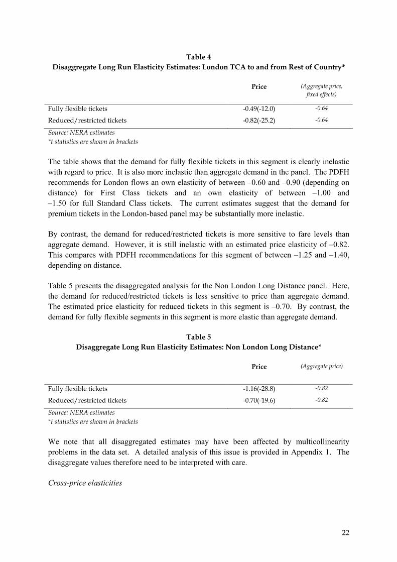
Table 4 Disaggregate Long Run Elasticity Estimates: London TCA to and from Rest of Country*
Price (Aggregate price, fixed effects)
Fully flexible tickets -0.49(-12.0) -0.64
Reduced/restricted tickets -0.82(-25.2) -0.64
Source: NERA estimates *t statistics are shown in brackets
The table shows that the demand for fully flexible tickets in this segment is clearly inelastic with regard to price. It is also more inelastic than aggregate demand in the panel. The PDFH recommends for London flows an own elasticity of between –0.60 and –0.90 (depending on distance) for First Class tickets and an own elasticity of between –1.00 and –1.50 for full Standard Class tickets. The current estimates suggest that the demand for premium tickets in the London-based panel may be substantially more inelastic.
By contrast, the demand for reduced/restricted tickets is more sensitive to fare levels than aggregate demand. However, it is still inelastic with an estimated price elasticity of –0.82. This compares with PDFH recommendations for this segment of between –1.25 and –1.40, depending on distance.
Table 5 presents the disaggregated analysis for the Non London Long Distance panel. Here, the demand for reduced/restricted tickets is less sensitive to price than aggregate demand. The estimated price elasticity for reduced tickets in this segment is –0.70. By contrast, the demand for fully flexible segments in this segment is more elastic than aggregate demand.
Table 5 Disaggregate Long Run Elasticity Estimates: Non London Long Distance*
Price (Aggregate price)
Fully flexible tickets -1.16(-28.8) -0.82
Reduced/restricted tickets -0.70(-19.6) -0.82
Source: NERA estimates *t statistics are shown in brackets
We note that all disaggregated estimates may have been affected by multicollinearity problems in the data set. A detailed analysis of this issue is provided in Appendix 1. The disaggregate values therefore need to be interpreted with care.
Cross-price elasticities

23
Our disaggregated analysis has allowed us to derive cross-price elasticity estimates for the two panels. We report them here but note that they may not be robust due to possible multicollinearity problems (see Appendix 1).18 As we have argued above, we believe that cross-price elasticities should in general be estimated using stated preference analysis based on survey work, the results of which can then be used as constraints on the cross-elasticities in the econometric model.
Our cross-price elasticity estimates for the London TCA to and from Rest of Country panel are shown in Table 6. The interpretation of the values in the table is that if, for example, the price of restricted/reduced tickets rises by 10 per cent, and the price of fully flexible tickets remains unchanged, the demand for fully flexible tickets rises by 1.5 per cent. If on the other hand the price of fully flexible fares rises by 10 per cent, and the price of restricted/reduced tickets remains constant, the demand for reduced tickets rises by 2.6 per cent. 19
Table 6 Long Run Cross-Price Elasticity Estimates: London TCA to and from Rest of Country*
Fully flexible price Reduced/restricted price
Demand for fully flexible tickets -0.49(-12.0) 0.15(3.7)
Demand for reduced/restricted tickets 0.26 (8.4) -0.82(-25.2)
Source: NERA estimates *t statistics are shown in brackets.
Table 7 contains our long-term estimates for the Non London Intercity segment. The results suggest that the substitutability of the two ticket type categories in this segment is significant. If reduced fares increase by 10 per cent, the demand for fully flexible tickets would increase by 7.4 per cent. The estimated of the demand for reduced tickets with respect to full fare levels is 0.48.
18 The cross-price elasticities that we report here are significant in that the relevant coefficients have high t-values. However, in the presence of multicollinearity, a result being significant in terms of having a high t-value does not imply that it is also accurate, and whilst we report the t-values in this section, we believe these should be treated with caution. Whether cross-price elasticities in the presence of multicollinearity can be used is ultimately a matter of judgment and cannot be determined on the basis of a single “significance” figure.
19 Given that the reduced/restricted segment is much larger in volume terms than the fully flexible segment, one would expect the cross-price elasticity of the demand for fully flexible tickets with respect to the price of reduced/restricted tickets to be larger than the cross-price elasticity of the demand for reduced/restricted tickets with respect to the price of fully flexible tickets. In our estimates, the opposite is the case, suggesting they may not be robust.

24
Table 7 Long Run Elasticity Estimates: Non London Long Distance*
Fully flexible price Reduced/restricted price
Demand for fully flexible tickets -1.16(-28.8) 0.74(13.3)
Demand for reduced/restricted tickets 0.48 (17.7) -0.70(-19.6)
Source: NERA estimates *t statistics are shown in brackets
Income Elasticity of Demand
Table 8 shows our estimates of the long run income (GDP) elasticity of aggregate demand for the two panels. Table 9 shows the estimated income elasticities of demand for the two groups of tickets included in the disaggregrated analysis.
Table 8 Long Run Income Elasticity of Aggregate Demand*
London TCA to and from rest of country
1.64 (82.3)
Non London long distance 1.76 (85.1) Source: NERA estimates t-statistics shown in brackets
Table 9 Long Run Income Elasticity of Demand by Ticket Type*
Ticket Type
Fully Flexible Reduced/Restricted
London TCA to and from rest of country
0.84(19.6) 1.78(55.8)
Non-London long distance 1.90(37.6) 1.29(37.1) Source: NERA estimates *t-statistics are shown in brackets
The results indicate that the demand for long distance rail travel in Great Britain is income elastic, in line with the findings from NERA’s previous work for OPRAF. The results from the two NERA studies contrast strongly with those obtained in the earlier research by Jones and Nichols and Owen and Phillips, which found no evidence that inter-city rail demand was significantly income elastic.

25
The Impact of the Hatfield Accident
While our research has focused on long-term elasticities, it has been necessary to take account of the impacts of the Hatfield accident and the subsequent disruption on demand. We have also examined the issue of the stability of the demand parameters by estimating equations both for the period prior to the Hatfield accident, and for the entire period for which data are available.
The effect of the post-Hatfield disruption on rail demand
For the reasons discussed earlier, we have attempted to estimate the effect of the post-Hatfield disruptions by using dummy variables in levels, which represent demand impacts in terms of a change in the constant term in the regression equation when the dummy variable is “on”. We have specified two dummy variables in our equations, one covering the first three four-weekly periods (i.e. weeks 1 to 12) after the accident, the other one covering the second three (i.e. weeks 13 to 24). In this way, most of the impact of the accident should be captured by the dummy variables without impacting on our elasticity estimates.
The values of the dummy variables are interesting in their own right, since they give insight into both the magnitude and the pattern of impact of the demand shock after the accident.
The impact of the accident and subsequent disruptions to rail services on aggregate demand in each panel is shown in Table 10. It should be emphasised that the figures reported in the table only show the impact on demand that is directly due to the accident. Other impacts of demand, such as seasonal changes, changes in fares or GDP, have been isolated from these figures as they are accounted for by other variables in our equations.
Table 10 Change in Aggregate Demand Due to Hatfield Accident*
(%)
In week 1 to 12 after the accident
In week 13 to 24 after the accident
London TCA to and from Rest of Country -24.7 (-8.1) -15.9 (-6.0)
Non London Long Distance -28.3 (-16.5) -15.2 (-9.0)
Source: NERA estimates *t-statistics are shown in brackets
As expected, the impact in the period immediately following the accident, when service disruptions were most pronounced, was substantially greater than in the later period.
Parameter stability

26
To test the robustness of our elasticity estimates, we have also estimated models for each panel in which only the period up to the Hatfield accident was analysed. Encouragingly, as shown in the full estimation results for aggregate demand equations presented in Appendix 3, we found that in both cases, the elasticity values for the pre-Hatfield period were very close to those estimated for the entire period.
Short Run Demand Response
We have reported the short and long term elasticities estimated using the Vector Error Correction Model (VECM). One of the attractive properties of this model is that it can also be used to estimate the speed with which the demand for rail travel adjusts to its long-term values. An overview of the insights arising from this analysis is provided in Table 11.
Table 11 Speed of Adjustment of Demand
London TCA to and from Rest of Country
Non-London Long Distance
Value of the adjustment factor 0.277 0.174
Proportion of demand change occurring within four weeks 28% 17%
Proportion of demand change occurring within six months 88% 71%
Proportion of demand change occurring within one year 99% 92%
Amount of time required for the change in demand to adjust to within 1 per cent of its long-term value
1 yr 1 month
1 yr 10 months
Source: NERA estimates
As can be seen in the table, our estimates suggest that elasticities of demand in the rail sector approach their long run values over a period of between one and two years, depending on the type of flow. The table also suggests that for both panels, more than 90 per cent of the demand adjustment occurs within a year after the fares change. Even in the case of the Non London Long Distance panel, where it takes almost two years for demand to adjust to its long run level, about 92 per cent of this adjustment occurs within the first year.
Conclusions
The econometric results presented above indicate that the long-run elasticity of demand with respect to fares is around –0.6 to –0.7 for longer distance rail journeys between the London area and the rest of Great Britain. For longer distance journeys between major urban areas other than London, our estimates indicate, in line with our prior expectations, a somewhat higher (more negative) elasticity of demand of around –0.8 to

27
–1.0. Both sets of estimates are close to those derived in previous research by NERA. Our results, which have potentially important implications for policy on rail fare regulation in these market segments, indicate that demand for rail travel between London and the rest of the country may be somewhat less price elastic than the values currently recommended in the PDFH, although our findings in respect of non-London travel are broadly in line with current industry planning assumptions.
The VECM results suggest that the long-run elasticity of demand is around three to five times the value of the short run elasticity, and that well over 90% of the long run demand adjustment occurs within 12 months of a demand shock, such as a change in real fares.
As well as examining the demand for rail travel aggregated over all types of ticket, we have also explored both the own- and cross-price elasticities of demand for different types of ticket. We found that for travel to and from the London area, the own-price elasticity of demand for reduced fare and restricted availability tickets was approximately twice as high as the own-price elasticity of demand for fully flexible tickets. For non-London journeys, however, the demand for fully flexible tickets was price elastic, and was higher than the own-price elasticity of demand for reduced fare/restricted availability tickets. Our estimates of the relevant cross-price elasticities were correctly signed, but the relative magnitudes of the parameter estimates for the London panel were not consistent with Slutsky symmetry conditions.
In general, whilst we regard our estimates of aggregate demand elasticities in both panels as highly robust, we have less confidence in the disaggregated own- and cross-price elasticities, because the data sets used to derive them are characterised by quite a high degree of multicollinearity.
Although the main focus of our research has been on the long run fare elasticities, our models have also produced estimates of the income elasticity of demand, and of the impact of the Hatfield accident on the demand for rail travel.
We find, consistent with estimates produced in previous work by NERA, that the income elasticity of demand at both aggregate and disaggregate levels is significantly positive, with aggregate demand in both market segments estimated to increase at over one and a half times as fast as the growth in GDP. This represents a very striking change from the results of studies of the demand for long distance rail travel carried out in the 1980s,20 in which the estimated income elasticity of demand was not significantly different from zero. We believe this apparent change in the market environment for rail
20 See, for example, Owen and Phillips (1987), and Jones and Nichols (1983).

28
travel may be linked to a deterioration in the quality of service available on the road network, where capacity growth has failed to keep up with growth in demand. 21
Finally, we find that the service disruptions following the Hatfield accident had a very major effect on the demand for rail travel. Our estimates indicate that in the three months immediately after the accident, demand was reduced by approximately a quarter; although there was some recovery in the following three months, continuing reductions in service quality were still resulting in a fall in demand of around 15%.
Overall, we regard the present exercise as demonstrating that the application of modern econometric methods to an exceptionally rich data set can yield robust and policy relevant estimates of key rail demand parameters.
Acknowledgements: The authors are grateful to Preetum Domah and his colleagues at the UK Strategic Rail Authority (SRA) for assistance in accessing and interpreting rail traffic and revenue data (held in the CAPRI database) and for helpful comments on draft material. The research on which the paper is based was funded by the SRA.
References
Dargay J. M. and M. Hanly (2002), “The Demand for Local Bus Services in England”, Journal of Transport Economics and Policy, 36(1), pp. 73-91
Im, Kyung So, M. Hashem Pesaran and Yongcheol Shin (2003), "Testing for Unit Roots in Heterogeneous Panels" Journal of Econometrics, 115, pp.53-74.
Jones, Ian S. (2001), “Railway Franchising: is it Sufficient? On-Rail Competition in the Privatized Passenger Rail Industry”, in Robinson, C. (editor), Regulating Utilities: New Issues, New Solutions, Edward Elgar, 2001
Jones, Ian S. and Alan J. Nichols (1983), “The Demand for Intercity Rail Travel in the United Kingdom. Some Evidence”, Journal of Transport Economics and Policy, 17 (2), pp.133-153
McCoskey, Suzanne and Chihwa Kao (1998) "A Residual-Based Test of the Null of Cointegration in Panel Data," Econometric Reviews, 17 (1), pp.57-84
NERA (1999), “Analysis of Passenger Rail Demand” A report for OPRAF, July
Owen, A.D. and G.D.A. Phillips (1987) “The Characteristics of Railway Passenger Demand: An Econometric Investigation”, Journal of Transport Economics and Policy, 21 (3), pp.231-253
21 See, Jones (2001) for further discussion.

29
Pedroni, Peter (1999), “Critical Values for Cointegration Tests in Heterogeneous Panels with Multiple Regressors”, Oxford Bulletin of Economics and Statistics, 61, pp.653-70

30
Appendix 1: Testing for Cointegration and Multicollienearity
Cointegration
To test for cointegration, it is usual first to establish the order of integration of the variables in question, and then - having established that the variables are of the same order of integration – to test whether there is at least one linear relationship among these variables.
To establish the order of integration of our explanatory variables, we have conducted panel unit root tests both for individual flows and for the whole panels. In general the individual flows test results suggest that the series are I(1) for all sectors and for our preferred set of explanatory variables. Furthermore, as the use of a panel increases the power of tests we apply the Im, Pesaran and Shin (2003) test for integration.22 These results provide strong evidence that all our series are I(1).
Having established the order of integration of our series, we proceed with tests for co-integration. The literature observes a variety of possible ways in order to test for cointegration. Regarding the time series studies, it is found that extending the time series data length affects the order of integration and number of cointegrating vectors. However, testing for cointegration in panels is less pressing, because the spurious regression problem is reduced by the averaging. Some of the most popular cointegration tests for panel data are the McCoskey and Kao (1998) methodology and the Pedroni (1999) methodology. The assumption of heterogeneity between different flows remains while testing for cointegration in panel data.
McCoskey and Kao (1998) use a Lagrange Multiplier test on the residuals that takes the following form:
ititiiti exay ++= β, (i)
where,
22 The Im, Pesaran and Smith (1997) t-bar test averages the test statistics for the individual countries, and standardizes this average test statistic by its expected value and variance under the null hypothesis. The resulting standardized test statistic, denoted Ψ-bar statistic, is distributed as standard normal for large N, and its formula is:
∑
∑
=
=
−=Ψ
N
iiT
N
iiTNT
tVARN
tEN
tN
1
1
][1
][1(
where tNT-bar is the average of the N individual ADF test statistics and E[tiT] and VAR[tiT] are the empirical first and second moments of the ADF test statistics under the null.

31
∑ =+=
t
j itijit uue1
θ (ii)
McCoskey and Kao (1998) consider the above model under the null Ho: θ = 0, ie that there is is cointegration in the panel, since for θ = 0, eit = uit and the above regression is a system of cointegration. The alternative Hα: θ ≠ 0, tests for a lack of cointegration. The statistics are obtained by using the model that follows:
2
1
2
12
11
+
=
+
=∑ ∑=
S
STNLM
N
i it
T
T (iii)
where S is the sum of the estimated error terms.
The estimation of the residuals can be applied by using OLS estimators and more specifically with the use of either FMOLS (Fully Modified OLS) or the DOLS (Dynamic OLS) estimator.
Pedroni (1999) also applies the cointegration test to the residuals of the regressions and uses the same Lagrange Multiplier test expressed in (iii) for a heterogeneous panel. Pedroni’s approach is different to that of McCoskey and Kao, and involves testing for a lack of cointegration in the panel. In this case the null is Ho: θ ≠ 0. In his analysis Pedroni proposes seven different cointegration statistics in order to capture the within and the between effects in his panel. All seven different statistics were calculated for our panels and the results indicated that in all cases, we have strong evidence of existence of cointegrating relationships.
Multicollinearity
The results obtained in the estimation of the disaggregated elasticities and cross-elasticities must be interpreted with care, because of the presence of multicollinearity among the measured explanatory variables that have been used for the disaggregate analysis of the four panels. Multicollinearity indicates that the explanatory variables are highly intercorrelated (i.e. there exists a strong linear relationship among some or all of the explanatory variables), leading to a lack of accuracy in estimating the effects that the explanatory variables produce on the dependent variable (i.e. the elasticities of the model). If this data problem occurs, the regression analysis is not able to precisely allocate the impact of the explanatory variables on the dependent variable, since some or all of those explanatory variables are approximately similar to a linear combination of the other explanatory variables. In other words, if multicollinearity exists, the estimates of the coefficients may have an unexpected sign or an implausible magnitude.
This data problem cannot be overcome easily. An approach that is sometimes pursued is dropping one or more of the regressors that produce the multicollinearity. We have not been able to do this, firstly, because one of the objectives of the project was to try to estimate the

32
cross-price elasticities, and secondly because, as we demonstrate, the potential multicollinearity problem may be due to the correlation between the series of the ticket prices.
We have examined the evidence on the existence of multicollinearity in the two panels. In order to do so, three measures have been calculated for each panel. These are:
• The correlation coefficients (ρ)23 between the different pairs of regressors. This coefficient takes values in the numerical range [-1,1]. The closer to 1 the absolute value of the ρ is, the stronger the evidence of multicollinearity is;
• The Variation Inflation Factor (VIF)24 for the different regressors. This factor takes values in the numerical range [1,+∞]. The higher the value of the VIF is, the stronger the evidence of multicollinearity is;25 and
• The measure of tolerance (TOL)26 for the different regressors. This measure takes values in the numerical range [0,1]. The closer the value of the TOL to 0 is, the stronger is the evidence of multicollinearity.
Tables 12 and 13 show that the main source of the multicollinearity problem is related to the linear relationship between the series of alternative ticket types. For these variables, the ρs take a value higher than 0.80; the VIFs are well above 1; and the TOLs are close to zero. The
23 The ρ is the ratio between the (i) covariance between the pair of regressors, and (ii) product of their standard deviations. The coefficient measures how strong is the linear relationship between the pair of regressors.
24 The VIF is a measure that can guide in identifying multicollinearity. To develop this concept it is useful to note that the variance of the OLS estimator for a typical regression coefficient (say βi) can be shown to be the following:
Var(βi) = σ2/Sii (1-Ri2)
Where (i) σ2 is the variance of the error term of the model, (ii) Sii is the sum of the differences to the square between the observations of the explanatory variable i and its arithmetic average, and (iii) Ri2 is the unadjusted R2 when the explanatory variable i is regressed against the other explanatory variables in the model.
The intuitive insight of this expression is that the stronger the linear relationship between the explanatory variables (i.e. multicollinearity) is, the larger the variance of the estimates of the regressions coefficients (and consequently the more difficult to obtain an accurate estimate of the true value of the parameter). In particular, if Ri2 is equal to 0, then the variance of the estimation takes its minimum possible value, which is σ2/Sii. Dividing this last expression into the above expression for Var(βi), the VIF is obtained.
VIF = 1/(1-Ri2)
It is straightforward to understand that the higher the VIF is, the lower the accuracy of the estimates of the parameter.
25 There is not a defined threshold for this factor as it is not based on any probability distribution. Nevertheless, as a rule of thumb, if the VIF exceeds 10 (i.e. the R2 of the auxiliary regressions exceeds 0.90), there is strong evidence of multicollinearity.
26 The TOL is defined as:
TOL(βi) = 1/VIF = 1- Ri2
It is clear that the lower is the TOL, the lower is the accuracy of the estimates of the parameter.
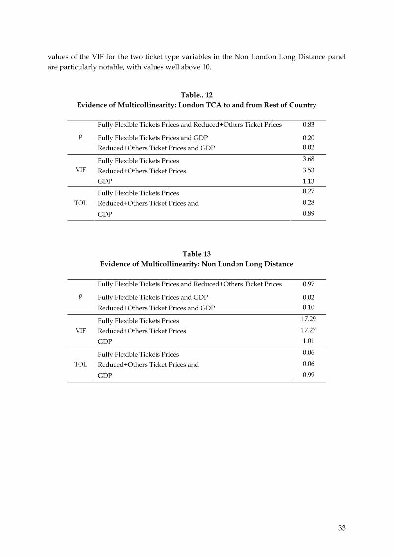
33
values of the VIF for the two ticket type variables in the Non London Long Distance panel are particularly notable, with values well above 10.
Table.. 12 Evidence of Multicollinearity: London TCA to and from Rest of Country
Fully Flexible Tickets Prices and Reduced+Others Ticket Prices 0.83
Fully Flexible Tickets Prices and GDP 0.20 ρ
Reduced+Others Ticket Prices and GDP 0.02
Fully Flexible Tickets Prices 3.68
Reduced+Others Ticket Prices 3.53 VIF
GDP 1.13
Fully Flexible Tickets Prices 0.27
Reduced+Others Ticket Prices and 0.28 TOL
GDP 0.89
Table 13 Evidence of Multicollinearity: Non London Long Distance
Fully Flexible Tickets Prices and Reduced+Others Ticket Prices 0.97
Fully Flexible Tickets Prices and GDP 0.02 ρ
Reduced+Others Ticket Prices and GDP 0.10
Fully Flexible Tickets Prices 17.29
Reduced+Others Ticket Prices 17.27 VIF
GDP 1.01
Fully Flexible Tickets Prices 0.06
Reduced+Others Ticket Prices and 0.06 TOL
GDP 0.99

34
Appendix 2: Traffic Flows and Ticket Types Included in the Analysis
Traffic Flows
Tables 14 and 15 show respectively the traffic flows used in the London and non-London panels.
Table 14 Origin-Destination Pairs: London TCA to and from the Rest of Country
Origin Zone Destination Zone 000 London 572 Bath 000 London 300 Birmingham 000 London 570 Bristol 000 London 550 Cardiff 000 London 170 Carlisle 000 London 950 Edinburgh 000 London 960 Glasgow 000 London 230 Leeds 000 London 400 Leicester 000 London 130 Liverpool 000 London 100 Manchester 000 London 200 Newcastle 000 London 460 Norwich 000 London 410 Nottingham 000 London 510 Plymouth 000 London 150 Preston 000 London 103 Stockport 000 London 540 Swansea 000 London 580 Swindon 000 London 220 York

35
Table 15 Origin-Destination Pairs: Non London Long Distance
Origin Zone Destination Zone 57 Avon 30 West Mids inner 57 Avon 42 Derby 57 Avon 13 South Merseyside 57 Avon 10 South Manchester 57 Avon 29 South Yorkshire 23 Leeds area 30 West Mids inner 23 Leeds area 42 Derby 23 Leeds area 13 South Merseyside 23 Leeds area 10 South Manchester 23 Leeds area 29 South Yorkshire 40 East Mids south 30 West Mids inner 40 East Mids south 42 Derby 40 East Mids south 13 South Merseyside 40 East Mids south 10 South Manchester 40 East Mids south 29 South Yorkshire 20 Tyne & Wear 42 Derby 20 Tyne & Wear 13 South Merseyside 20 Tyne & Wear 10 South Manchester 20 Tyne & Wear 29 South Yorkshire 41 Nottingham 30 West Mids inner 41 Nottingham 42 Derby 41 Nottingham 13 South Merseyside 41 Nottingham 10 South Manchester 41 Nottingham 29 South Yorkshire 45 Peterborough 47 Ipswich 30 West Mids inner 45 Peterborough 23 Leeds area 95 Edinburgh area 54 South Wales 57 Avon 17 Carlisle 34 Stoke 17 Carlisle 20 Tyne & Wear 23 Leeds area 27 North Humber 95 Edinburgh area 96 Glasgow inner 38 Rugby 96 Glasgow inner 21 Teesside 51 West Devon
Ticket Types
Table 16 shows how individual types of ticket were allocated between the ticket categories used in the disaggregated demand analysis.

36
Table 16 Disaggregation by Ticket Type
London TCA to and from Rest
of Country
Non-London Long Distance
1ST/EXEC STD SINGLE STD/OPEN RTN
First+Standard First+Standard
SAVER SUPERSAVER NETWWK AWYBRK APEX DAY RETURN ANNUAL S/T WEEKLY S/T OTHER SEASON SLEEPER SUPP CHDY SINGLE
Ticket types
OTHER
Reduced+Other Reduced+Other
Appendix 3: Detailed Estimation Results for Aggregate Models
Tables 17 and 18 show respectively the detailed estimation results for the London and non-London panels. The tables each include results for the entire estimation period and for the period before the Hatfield accident.
Table 17 Detailed Aggregate Estimation Results: London TCA to and from Rest of Country
Period up to Hatfield Entire period Estimate t-statistic Estimate t-statistic Price -0.64 -22.9 -0.64 -26.1 GDP 1.71 67.5 1.64 82.3 S_1 -0.09 -8.7 -0.09 -8.6 S_2 -0.03 -2.5 -0.03 -3.0 S_3 -0.05 -4.2 -0.05 -4.5 S_4 0.00 -0.2 0.00 0.0 S_5 -0.10 -8.7 -0.10 -9.3 S_6 -0.13 -11.2 -0.13 -12.3 S_7 -0.02 -1.8 -0.02 -2.2 S_8 0.06 5.0 0.06 5.6 S_9 0.08 7.5 0.08 7.5 S_10 -0.16 -14.2 -0.17 -17.1 S_11 -0.14 -12.6 -0.14 -13.6 S_12 -0.01 -1.0 0.00 -0.4 Hat_1 - - -0.25 -8.1 Hat_2 - - -0.16 -6.0

37
Source: NERA estimates
Table 18 Detailed Aggregate Estimation Results: Non London Long Distance
Period up to Hatfield Entire period
Estimate t-statistic Estimate t-statistic
Price -0.82 -37.8 -0.82 -41.8
GDP 1.59 61.5 1.76 85.1
S_1 -0.12 -11.1 -0.12 -11.8
S_2 -0.09 -8.8 -0.09 -9.6
S_3 -0.10 -9.5 -0.10 -10.1
S_4 -0.11 -10.7 -0.11 -10.7
S_5 -0.16 -14.8 -0.15 -14.8
S_6 -0.15 -14.4 -0.15 -14.8
S_7 -0.05 -4.7 -0.04 -4.1
S_8 0.06 5.7 0.07 7.0
S_9 0.05 4.6 0.05 5.1
S_10 -0.15 -14.2 -0.17 -17.6
S_11 -0.13 -12.6 -0.14 -14.2
S_12 0.02 1.8 0.02 2.2
Hat_1 - - -0.28 -16.5
Hat_2 - - -0.15 -9.0
Source: NERA estimates
Notes
S_1, S_2 etc are seasonal dummy variables. Hat_1 is a dummy variable taking the value 1 in time periods 1 to 3 after the Hatfield accident, and zero otherwise. Hat_2 is a dummy variable taking the value 1 in time periods 4 to 6 after the Hatfield accident, and zero otherwise.