Embed Size (px)
Citation preview

DEPARTMENT OF ECONOMICS
Working Paper
Labor Productivity and the Law of Decreasing Labor Content
By
Peter Flaschel, Reiner Franke and Roberto Veneziani
Working Paper 2010‐11
UNIVERSITY OF MASSACHUSETTS AMHERST

Labor Productivityand the Law of Decreasing Labor Content∗
Peter Flaschel† Reiner Franke‡ Roberto Veneziani §
August 3, 2010
Abstract
This paper analyzes labor productivity and the law of decreasing labor con-tent (LDLC) originally formulated by Farjoun and Machover (1983). First,it is shown that the standard measures of labor productivity may be rathermisleading, owing to their emphasis on monetary aggregates. Instead, theconventional classical-Marxian labor values provide the theoretically and em-pirically sound measures of labor productivity. The notion of labor contentand the LDLC are therefore central in order to understand the dynamics ofcapitalist economies. Second, some rigorous theoretical relations between dif-ferent forms of profit-driven technical change and productivity are derived ina general input-output framework with fixed capital, which provide determin-istic foundations to the LDLC. Third, the main theoretical propositions areanalyzed empirically based on a new dataset of the German economy.———————Keywords: labor productivity, law of falling labor content, technical change,labor values, Input-Output analysis.
JEL CLASSIFICATION SYSTEM: B51 (Socialist; Marxian; Sraffian),D57 (Input-Output Analysis), O33 (Technological Change: Choices and Con-sequences), C67 (Input-Output Models).
∗We are grateful to Clopper Almon, Theodore Mariolis and Simon Mohun for comments and sug-gestions. Roberto Veneziani worked on this project while visiting the University of Massachusetts,Amherst. Their hospitality is gratefully acknowledged. The usual disclaimer applies.
†(Corresponding author) Department of Business Administration and Economics, BielefeldUniversity, P.O. Box 10 01 31, 33501 Bielefeld, Germany. Tel: +49-521- 123075. E-mail:[email protected]
‡Faculty of Economics, Kiel University, Germany. Address: Hauffstrasse 17, 28217 Bremen.Tel: ++49-421-3965447. E-mail: [email protected]
§Department of Economics, Queen Mary University of London, Mile End Road, London E14NS, UK. Tel: +44-20-78828852. E-mail: [email protected]

1 Introduction
In their influential book on Laws of Chaos, Farjoun and Machover (1983) formulatethe celebrated law of decreasing labor content (henceforth, LDLC). According to theLDLC, if C is a commodity produced in a capitalist economy over a certain period oftime, then “there is virtual certainty (probability very near 1) that the labor contentof one unit of C will be lower at the end of the period than it was at the beginning”(ibid., p.97). According to Farjoun and Machover, the LDLC is a defining featureof capitalist economies: it is “the most basic dynamic law of capitalism, archetypeof all capitalist development” (ibid., p.139).
Granting that the LDLC characterizes capitalist economies, two questions immedi-ately arise. First, why is the LDLC relevant from a theoretical viewpoint? Farjounand Machover consider the LDLC as self-evidently relevant because they see it asequivalent to the law of increasing labor productivity (see, for example, ibid., pp.11,139 and passim). And labor productivity plays a key role in economic theories ofgrowth and employment, including issues of innovation, structural change, incomedistribution, and so on. Yet the relevance of the LDLC for understanding trendsin labor productivity is far from obvious: virtually all of the received productiv-ity measures - as developed for instance in the UN’s System of National Accounts(henceforth, SNA; UN, 1993. See also OECD, 2001; BLS, 2008) - focus on real GDPper unit of labor, or on some notion of ‘real value added’ per unit of labor, in order tomeasure the performance of (different sectors of) the economy. If the conventionalSNA measures properly capture labor productivity, then one may argue that thenotion of labor content is either misleading or at best redundant: the LDLC mayindeed be “a prime example of a tendency that operates ‘behind the backs’ of thesocial protagonist, as though it were a law of nature” (Farjoun and Machover, 1983,p.84), but in order to explain some fundamental features of capitalist economies itwould be unnecessary to uncover “some systematic connection between the visibleand the invisible - between price and labor-content” (ibid.). It would be sufficient toanalyze the dynamics of the price-based SNA measures. In other words, in principle,the relevance of the law of increasing labor productivity says very little about therelevance of the LDLC.
The second question is, how can the LDLC be derived, or deduced, from the func-tioning of capitalist market economies? What is the mechanism which explains “whyindividual actions motivated by considerations of price should in the long term re-sult in a systematic effect on labor-content” (ibid., p.84)? Farjoun and Machoverprove that the LDLC obtains in a probabilistic framework as the cumulative resultof a sequence of technical changes such that the cost of physical inputs decreaseswhile labor inputs remain constant. This type of innovations, however, represent arather special case of the range of technical changes adopted in capitalist economies.Besides, the behavioral foundations of their analysis are not entirely spelled out, andfixed capital plays no essential role in their model, even though it is arguably centralin capitalists’ innovating decisions.
This paper analyzes both questions in a general input-output (henceforth, IO) frame-work. Indeed, it is shown, contra Farjoun and Machover, that a generalized IOapproach provides a natural framework to formulate and derive the LDLC, and alsoto understand its theoretical relevance.
Section 2 addresses the first question and it shows the salience of the notion of laborcontent for the understanding of labor productivity. A thorough critical analysisof the standard SNA measures of sectoral as well as aggregate labor productiv-ity is provided, from an IO perspective. The analysis of the structural featuresof the economy allowed by the IO framework forcefully shows that the SNA mea-sures are inappropriate to capture production conditions, and shifts in efficiencyand technology, owing to the central role of relative prices and final demand in theirconstruction. Measures of sectoral and total labor productivity should be based ontechnological data as much as possible (subject to an unavoidable degree of aggre-gation), and they should not definitionally depend on price variables. Instead, theIO employment multipliers - that is, the labor values of classical-Marxian economictheory1 - provide (in reciprocal form) theoretically sound measures of sectoral andeconomy-wide labor productivity, with purely technological foundations - insofar asIO coefficients can be interpreted as pure quantity magnitudes.
Thus, section 2 proves that the law of increasing labor productivity cannot be prop-erly understood unless the LDLC is formulated. Yet the analysis also has broaderimplications for productivity analysis, because it shows that the shortcomings ofthe standard indices are more serious than it is acknowledged in the mainstreamliterature (e.g., Durand, 1994; Cassing, 1996; Schreyer, 2001) and that a proper un-derstanding of labor productivity requires a focus on labor content. IO tables shouldalways be an integral part of the SNA and the point of reference for all productivitymeasures at the macro- and meso-level of economic activity.2
Critiques of standard SNA productivity measures from an IO perspective and theuse of employment multipliers to measure productivity are not novel (see, amongthe others, Gupta and Steedman, 1971; Steedman, 1983; Wolff, 1985, 1994; de Juanand Febrero, 2000; Almon, 2009).3 This paper presents a new set of arguments anda unified theoretical framework for the analysis of productivity measures, which isbased on a novel axiomatic method. Rather than comparing different measures interms of their implications in various scenarios, this paper starts from first principlesand formalizes some theoretically desirable properties that any measure of laborproductivity should satisfy.4 To be precise, the main axiom focuses only on changes
1Total labor costs and employment multipliers are identical in Leontief models, but can differin more general economies. The analysis below can be extended to the general case by using theframework outlined in Flaschel (1983), albeit at the cost of a significant increase in technicalities.
2The importance of IO tables in productivity analysis is acknowledged in the mainstream liter-ature (see, for example, Schreyer, 2001, p.50).
3In Richard Stone’s original formulation of the UN’s (1968) SNA, it is possible to find definitionsof labor productivity that are conceptually analogous to the IO, or classical-Marxian, measures(e.g., UN, 1968, p.69). This paper suggests that it is quite unfortunate that this approach hasbeen abandoned in the following revisions.
4The adoption of an axiomatic approach to analyze classical-Marxian themes is quite novel. For
2

in productivity and states that labor productivity at t in the production of goodi has increased relative to the base period, if a unit increase of the net productof good i demands less labor than in the base period. This is a weak restrictionand it incorporates the key intuitions behind the main productivity measures inthe literature. Yet it characterizes the IO measures, whereas the conventional SNAindices do not satisfy it in general owing to their inherent dependence on relativeprices and final demand.
The second major contribution of this paper, in section 3, is a rigorous analysis ofthe conditions under which profitable innovations lower labor values, thereby raisingproductivity and increasing consumption and investment opportunities. Accordingto Farjoun and Machover (1983, p.141), “In [IO] theories of prices and profit thenotion of labor-content can be defined, and the law can certainly be formulated.But it cannot be deduced or explained, because in these theories there is no generalsystematic connection between labour-content and price”. This paper shows thatthis conclusion is not entirely correct and some systematic, deterministic connectionsbetween prices and labor content can be derived in general linear economies withfixed and circulating capital within the classical-Marxian tradition.
To be precise, in this paper the n-commodity general equilibrium models analyzedby Roemer (1977, 1980) are generalized into two main directions. First, followingthe approach developed by Flaschel (2010), the circulating capital model is extendedto the treatment of fixed capital proposed by Brody (1970) in a seminal contribu-tion. This is important because fixed capital - or, more precisely, capital tied up inproduction - is a key feature of capitalist economies and it is at the center of inno-vation processes but, as various authors have argued, the standard von Neumannframework has serious theoretical and empirical limitations.5 Second, the analysisdoes not depend on any assumptions on prices: no condition on uniform profit ratesis imposed and the conclusions hold for any vector of prices measured in terms of thewage unit. This extension is both empirically and theoretically relevant, becausegeneral equilibrium-type constructions (including uniform profit rate models) maybe unsatisfactory as representations of allocation in market economies as argued,among the others, by Farjoun and Machover (1983).
In this general framework, different forms of technical change can be considered,and a deterministic theoretical foundation for the LDLC can be derived. In fact, itcan be proved that profitable fixed-capital–using labor–saving innovations lead toproductivity increases. Given that capital–using labor–saving technical change hascharacterized most of the phases in the evolution of capitalism (Marquetti, 2003),this result provides theoretical foundations for the conclusion that labor values tendto fall, and labor productivity tends to rise, over time in capitalist economies.6 Theformal analysis has also broader implications concerning the social effects of capital-
a seminal contribution, see Yoshihara (2010).5See Brody (1970) and more recently, Flaschel et al. (2010). For an extension of Roemer’s
(1977) model to von Neumann economies see Roemer (1979) and Dietzenbacher (1989).6These results are consistent with the Marxian analysis of technical change and the historical
tendencies of capitalism. See Foley (1986) and Dumenil and Levy (1995, 2003).
3
ists’ individual decisions. For it can be proved that there is no clear-cut relationshipbetween profitable technical change and social welfare in capitalist economies: cap-italists’ maximizing behavior is neither necessary nor sufficient for the implementa-tion of productivity-enhancing and welfare-improving innovations.
The analysis in section 3 is related to the classical literature on technical change,distribution, and the evolution of capitalism (for recent contributions, see Dumeniland Levy, 2003; Foley, 2003; Petith, 2008). Yet unlike in the latter contributions, anexplicit microeconomic perspective is adopted, which emphasizes capitalists’ profit-maximizing behavior in highly disaggregated economies. Moreover, although thepaper may shed some light on the influence of distributive conflict on technicalchange, the focus is not on the general relation between technical change and dis-tribution, or on the much-debated effect of technical progress on profitability (seealso Michl, 1994). Instead the effect of individually optimal capitalist decisions onproductivity and social welfare is thoroughly explored. Finally, although the processgenerating innovations is not explicitly formalized, the analysis presented here canbe supplemented with the classical-Marxian evolutionary model of technical changedeveloped by Dumenil and Levy (1995, 2003).
The analysis is not purely theoretical, though. In section 4, an empirical appraisalof the main theoretical conclusions is provided, based on the new IO dataset of theGerman economy constructed by Kalmbach et al. (2005). The empirical evidenceconfirms the main conclusions: first, SNA measures of labor productivity can berather misleading and quite different from the theoretically sound IO indices. Sec-ond, the LDLC holds for the German economy, a fact that is not easily visible byjust looking at the IO tables. It should be noted, however, that the main aim of thispaper is not to provide a fully rigorous econometric analysis of productivity mea-sures, or of long-term trends of technical change in capitalist economies. The focusis primarily theoretical and methodological: the paper provides a general analysisof the relationships between prices, technical change, and labor productivity. Fromthis viewpoint, the discussion of the German economy (1991-2000) does not aimto be exhaustive: it only illustrates the main theoretical points, and the empiricalresults should be taken as a first step towards a more detailed analysis.
2 Labor content and labor productivity
The point of departure of the analysis is the standard IO table 2, which showseconomic activity in a particular year in the n sectors of the economy. The notationis standard: p(t) = (p1(t), ..., pn(t)) is the 1×n vector of prices of the n commoditiesat time t; xij(t) is the amount of good i used as intermediate input in the productionof good j; xi(t) is the gross output of good i; fi(t) is the final demand of good i.
At the most general level, labor productivity can be defined as a ratio between anindex of output and an index of labor input. One possibility is to use gross output asa measure of real product and to define labor productivity as gross output per unit
4

Delivery from ↓ to → Sector 1 . . . Sector n Final Demand row sumSector 1 x11(t)p1(t) . . . x1n(t)p1(t) f1(t)p1(t) x1(t)p1(t)
· · · · ·· · · · ·· · · · ·
Sector n xn1(t)pn(t) . . . xnn(t)pn(t) fn(t)pn(t) xn(t)pn(t)Value Added Y1(t) . . . Yn(t) – Y (t)column sum x1(t)p1(t) . . . xn(t)pn(t) F (t)
Table 1: The standard form of an input-output table
of direct labor. As is well known, however, this measure is appropriate only in therather special case of technical progress affecting all factors proportionally. Further,gross output based indices of productivity are sensitive to the degree of verticalintegration: ceteris paribus, gross output based productivity rises as a consequenceof outsourcing, even if there are no changes in technology and production conditions.
Therefore most of the literature focuses on value added.7 Two methods are used toobtain real output measures starting from value added data. The single deflationmethod requires deflating all entries (both outputs and inputs) in the nominal table2 by a common price deflator, say P . Single-deflated value added in sector i isthen Y s
i (t) = Yi(t)/P , and at the aggregate level Y s(t) =∑n
i=1 Ysi (t). Instead,
the method of double deflation attempts to measure everything in constant prices,that is, with regard to table 2 it attempts to replace current prices p(t) with theprices p(0) of a base year t = 0 . This method, however, cannot be directly appliedto the row of values added in table 2, which are pure value magnitudes, and thedouble deflated sectoral values added Y d
i (t) are obtained indirectly by applying theaccounting consistency requirement of the nominal table 2 to its analogue in constantprices. This means that Y d
i (t) is the value added that would have resulted in sectori, if the prices in table 2 had remained constant after the base year.
Thus, value added in base year prices remains a value magnitude and not a quantityindependent of relative prices, and therefore both single- and double-deflated valueadded are problematic notions in productivity analysis. “Value added is ... notan immediately plausible measure of output: contrary to gross output, there is nophysical quantity that corresponds to a volume measure of value-added” (Schreyer,2001, p. 41). Rather than measures of sectoral real output, single deflated values,Y si (t), should be interpreted as indices of sectoral real incomes, with only a distant
relation with technological conditions. Therefore any such measure as Y si (t)/Li(t)
- where Li(t) denotes the work hours employed in sector i - represents at best realpurchasing power per unit of labor, rather than sectoral labor productivity. Instead,the economic meaning of sectoral double deflated value added is rather unclear: sinceY di (t) in general differs from Y s
i (t), for any i, then Y di (t) does not measure output
7For an approach focusing on gross output, see Hart (1996) and Stiroh (2002).
5

\ 1 . . . n
1·· X f x·n
yd′
- Y d
x′
F d -
Table 2: Elementary input-output table in matrix notation
correctly, and in addition it has nothing to do with real purchasing power. It isa purely fictitious quantity representing the income per worker that would haveemerged if prices had remained constant at the level of the base year.
These well-known conceptual problems, though, are usually considered as minor,and in virtually all of the literature on labor productivity, value-added measuresof real output, and in particular the double-deflated values, Y d
i (t) and Y d(t), areused. Sectoral and macroeconomic labor productivity are defined, respectively, asπci (t) = Y d
i (t)/Li(t), and πc(t) = Y d(t)/L(t), where L(t) =∑n
i=1 Li(t), and πc(t)can be decomposed as follows:
πc(t) =∑i
(Li(t)
L(t)
)·(Y di (t)
Li(t)
)=
∑i
(Li(t)
L(t)
)· πc
i (t). (1)
Value added based indices are considered theoretically and empirically meaningful.Indices based on single-deflated value added are deemed appropriate to analyzeissues relating to economic welfare, whereas “for the purposes of measuring efficiencyand productivity [double deflated measures are] to be preferred” (Stoneman andFrancis, 1994, p.425; see also Cassing, 1996). Several doubts can be raised on bothclaims, and in general on the standard approach to productivity analysis.
For any vector z ∈ Rn, let z′ denote its transpose8 and let z denote the diagonalmatrix with z as its diagonal. In IO analysis, it is common to choose the units ofthe n commodities so that, in the base period, p(0) = e′ ≡ (1, ..., 1). The double orrow-wise ‘price deflated’ table 2 can then be expressed in matrix notation as in table2. Following common practice in IO analysis, the matrix of intermediate inputsX can be transformed into the matrix of input coefficients A = Xx−1, and the1× n vector of direct labor inputs ` = (`1, ..., `n) can be similarly transformed intoa vector of labor coefficients l = `x−1.9 Then, the macro-identity Y d = p(0)f = F d
behind table 2 can be expressed in matrix notation as follows
Y d = p(0)yd = p(0)(I − A)x = p(0)f = F d.
8In what follows, vectors are always column vectors, unless otherwise stated.9For the sake of notational simplicity, in the rest of the paper, the timing of vectors will be
omitted, whenever this is clear from the context.
6

Instead, the labor time spent, directly and indirectly, in the production of the ngoods is given by v = (v1, ..., vn) = l(I − A)−1 and the IO, or classical-Marxianmeasures of sectoral labor productivity are defined as πm
i = 1/vi.10 In the rest of
this section, a general framework is provided to compare productivity measures.In order to avoid problems of interpretation, the structural coefficients (A, l) areconsidered as the parameters of a linear technology, as in standard IO practice.
One of the key problems of the SNA measures is that they are sensitive to changes inrelative prices which do not reflect any shift in production conditions. Consider, forexample, a simple economy with one capital good and one pure consumption good,such that at a given period t the technical coefficients, aij, are 0 < a11 < 1, a12 > 0,and a21 = a22 = 0. If a single price deflator P is used, which includes prices of allsectors, as in standard index price theory, then quite puzzlingly real value added insector 1 may be affected by changes occurring in sector 2 even if good 2 does notenter the production of good 1, either directly or indirectly.11
Productivity indices based on double deflated value added fare no better. Considerthe IO matrix A in constant prices where the standard normalization p(0) = e′ is notadopted, so that aij = pi(0)aij/pj(0), for all i, j. Similarly, lj = lj/pj(0) and thusthe same relationship holds for labor values: vj = vj/pj(0). Because the investmentgood sector is homogeneous with respect to inputs and outputs:
πc1 =
1− p1(0)a11/p1(0)
l1/p1(0)=
1− a11l1/p1(0)
=p1(0)
v1,
so that relative prices do not distort πc1, which coincides with the IO measure. For
the consumption good sector, however, a different conclusion holds:
πc2 =
1− p1(0)a12/p2(0)
l2/p2(0)=
p2(0)− p1(0)a12l2
6=1
v2/p2(0)=
1
(v1/p1(0))p1(0)a12/p2(0) + l2/p2(0)=
1
(v1a12 + l2)/p2(0).
The numerator of πc2 depends on relative prices, and thus on their structure and on
the base period used. As a result, if p(0) changes, πc2 can change erratically without
any changes in production conditions. To be sure, labor values are also measuredrelative to output value, but this only means that each time series of labor values isdivided by the constant price of the corresponding good, which does not distort theinternal structure of the time series itself: for any given j, 1/vj is only rescaled andits growth rate is independent of prices. In general, whereas the indices πc
j dependon the conceptually dubious double deflated values added, the vector v is derivedfrom the meaningful, volume-oriented double deflated entries of the IO table A.
10v can be derived even if the assumptions of this paper are relaxed: see Gupta and Steedman(1971) for the treatment of fixed capital and imports, and Flaschel (1983) on joint production.
11In general, when output prices change relative to input prices, the single deflation method willdetect variations in productivity even if production conditions are unchanged. For related analysesof the sensitivity of the SNA measures to changes in relative prices see Durand (1994), Hart (1996);and Almon (2009).
7

The previous conclusions can be generalized and made more rigorous, by analyzingalternative approaches in a unified framework, in which some desirable properties ofproductivity measures are defined ex ante. Let ei = (0, ..., 1, ..., 0)′ be the i−th unitybase vector. Definition 1 formalizes the notion of increases in labor productivity.12
Definition 1 (D1)
1. Labor productivity at t has increased with regard to commodity i, relativeto the base period, if and only if an increase of the net product f by oneunit of commodity i demands less labor than in the base period. Formally, letxi(t) = (I−A(t))−1ei and let `i(t) = l(t)xi(t): labor productivity has increasedif and only if `i(t) < `i(0).
2. If `(t) ≤ `(0) then labor productivity at t has increased in the whole economy,with respect to the base period.
D1 does not aim to capture all aspects of labor productivity, and it only constrainschanges in productivity. From an epistemological viewpoint, it can be seen as anaxiom: whatever else a measure of productivity may do, it should satisfy D1, whichsets some minimal restrictions on productivity measures. From this perspective, D1has a number of attractive features. First, it has a firm technological foundationwhich captures only shifts in productive conditions and efficiency: purely monetarymagnitudes are irrelevant and final demand plays only an auxiliary role.13 This iscertainly a desirable property of labor productivity measures, as many authors haveargued (e.g. OECD, 2001). Second, by focusing on goods, rather than sectors, D1(1)incorporates the interdependencies between sectors and it allows one to capturethe relation between technical change and social welfare. This may seem morecontroversial, but a similar concern for the role of intermediate inputs and verticalintegration actually motivates the use of value-added based - as opposed to grossoutput based - indices in the mainstream literature (e.g. Schreyer, 2001, p.41ff):they are preferred because they capture interindustry transactions and “providean indication of the importance of the productivity measurement for the economyas a whole. They indicate how much extra delivery to final demand per unit ofprimary inputs an industry generates” (Schreyer, 2001, p.42). Third, D1(2) may bedeemed rather stringent, especially if n is large, as it requires (weakly) monotonicincreases for all goods. From an axiomatic perspective, however, it sets a very weakand intuitive restriction on any productivity measure. This is even more evidentif a (neoclassical) notion of productivity as measuring economic welfare is adopted,for in this case D1(2) is analogous to a paretian condition capturing vector-wiseimprovements in consumption and investment opportunities.
The next result states that D1 characterizes the classical-Marxian measures of laborproductivity.
12The following notation holds for vector inequalities: for all x, y ∈ Rn, x = y if and only ifxi = yi, all i; x ≥ y if and only if xi = yi and x 6= y; and x > y if and only if xi > yi, all i.
13The original net product f is irrelevant in D1, thanks to the linearity of the technology.
8
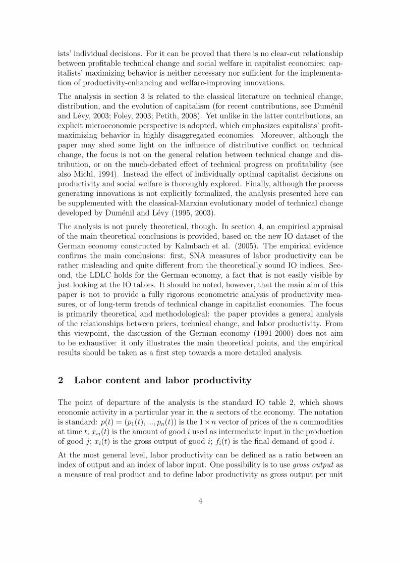
Proposition 1
For a given commodity i, `i(t) < `i(0) if and only if πmi (t) > πm
i (0).Furthermore, if the whole economy is considered `(t) ≤ `(0) if and onlyif πm
i (t) ≥ πmi (0), for all i = 1, . . . , n, with strict inequality for some i.
Proof:By the definition of v, L = `e = lx = l(I − A)−1f = vf. The latter expressionimplies li(t) = v(t)ei = vi(t) and the desired result follows.
In other words, labor productivity with regard to good i increases if and only if theamount of labor directly and indirectly embodied in good i decreases. Further, anyindex of aggregate labor productivity satisfies D1(2) if and only if it is monotonicin the vector of labor values. Proposition 1 provides theoretical foundations tothe classical-Marxian indices as the appropriate indicators of labor productivity.To be sure, one may argue that the indices πm
j have the disadvantage that theycannot be deduced only from data that characterize sector j, and it is this propertythat drives Proposition 1. Yet the standard value-added based measures cannot bedefined based only on data from sector j, either, even though the dependence onthe other sectors is less evident than in πm
j . It is in fact impossible to formulate andinterpret nominal value added Yj – as well as ‘real’ value added Y s
j , or Ydj – without
reference to a price system (even if prices may not appear explicitly, owing to thenormalization p(0) = e′). SNA measures do depend on the data of the other sectorsvia the price vector, but – unlike for πm
j – the sectoral influences are unexplained anddepend on the contingent institutional and market conditions of the base year. Therigorous technological foundation which characterizes the classical-Marxian indices islost. Therefore, it should not be surprising that the standard SNA measures cannotcorrectly capture labor productivity either at the sectoral or at the aggregate level.This is proved in the following propositions.
Proposition 2 states that the SNA and the classical-Marxian indices of sectoral laborproductivity coincide only in a very special case.
Proposition 2
The equality πcj = πm
j = 1/vj, for all j = 1, ..., n holds if and only ifπcj = πc, for all j = 1, ..., n.
Proof:The result follows immediately noting that πc
j = πc, all j = 1, ..., n, holds if and onlyif e′ − e′A = πcl, or equivalently (1/πc)e′ = l(I − A)−1 = v.
By Proposition 2, any differences in the two sectoral indices must be examined inrelation to sectoral productivity differences. The next result instead shows that theSNA measure of aggregate productivity satisfies D1(2), if final demand is constant.
9

structure \ period t = 0 t = 1
matrix of intermediate inputs A0.1 0.30.4 0.3
0.44 0.30.1 0.3
labor inputs l 0.4 0.05 0.32 0.05
Table 3: A two-sector economy with profitable capital-using and labor-saving tech-nical change (at constant prices p(0) = e′, w = 1)
Proposition 3
Suppose that f(t) = f(0) = f > 0. If v(t) ≤ v(0) then πc(t) > πc(0).Furthermore, πc(t) > πc(0) if and only if v(t)f < v(0)f .
Proof:The result follows noting that πc(t) = p(0)f/L(t) and that the equality L(t) = v(t)fholds, as shown in Proposition 1.
In other words, technical change yielding increases in productivity according toD1(2) implies a corresponding change in the SNA macroeconomic measure of laborproductivity. Further, the change in technology decreases the expenditure of humanlabor for the production of a given vector of final demand f . Thus, Proposition3 suggests that movements in the SNA aggregate measure map changes in the IOindicators, if final demand is constant. Yet Proposition 3 does not necessarily holdif final demand varies, nor does it hold at the sectoral level.
Consider the two-sector economy described in table 3, where process 1 is subjectto technical change between t = 0 and t = 1. Let p(0) = e′ and assume w = 1.First, technical change in sector 1 is capital-using and labor-saving, in the sense thatit increases the value of intermediate inputs, but it lowers labor costs, at currentprices. Second, technical change is profitable, because unit costs in sector 1 decreasefrom 0.9 to 0.86. Third, the SNA sectoral productivity measure increases in sector1 and remains constant in sector 2:
πc1(1) ≈ 1.44 > πc
1(0) = 1.25, πc2(1) = πc
2(0) = 8.
Instead, fourth, the classical-Marxian measures, πm1 , π
m2 , decrease:
πm1 (1) ≈ 1.58 < πm
1 (0) ≈ 1.70, and
πm1 (1) ≈ 3.04 < πm
1 (0) ≈ 3.09.
The technical change described in table 3 leads to a sharp divergence in the standardindices, πc
i , and the IO indices, πmi , which can move in opposite directions. Therefore,
by Proposition 1, the example in table 3 proves that the SNA sectoral measures,
10

πci , do not satisfy D1. Noting that these conclusions can be generalized to n-good
economies, they can be summarized in the next Proposition.14
Proposition 4
Suppose that f(t) = f(0) = f > 0. For any good i, if `i(t) < `i(0)then πc
i (t) may increase, decrease, or remain constant relative to πci (0).
Furthermore, it is possible to have `(t) ≤ `(0), but πci (t) 5 πc
i (0), for alli, with strict inequality for at least some i.
In other words, the standard sectoral productivity indices do not satisfy the minimalrequirements set out in D1, even under the restrictive assumption of a constant finaldemand. The shortcomings of the SNA measures πc
i derive primarily from the factthat they crucially rely on price information and do not properly reflect changesin technology. As a result, they can show increases in productivity in every sectoreven if the net production possibilities of the economy are deteriorating. Actually,by Proposition 3, the SNA aggregate index πc does correctly reflect changes in thewhole economy whenever final demand is constant, but table 3 shows that πc andthe sectoral measures πc
j can actually move in opposite directions (in the example,πc increases), if the sectoral allocation of labor changes appropriately (see equation1). Hence, the SNA sectoral measures do not provide useful information concerningthe sectors leading to movements in aggregate labor productivity.
It is worth stressing that the proof of Proposition 4 is completely general. In table3, only profitable technical change is considered, but this is unnecessary to estab-lish the proposition. It is however theoretically relevant because it shows that theresult is not driven by some peculiar, or economically meaningless, combination ofparameters. Further, none of the conclusions depends on the assumption of capital-using, labor-saving technical change, and it is easy to construct similar exampleswith other types of innovations.
Although the previous analysis has focused on sectoral productivity measures, thestandard approach to aggregate productivity is also unsatisfactory, and the SNAmeasure πc does not satisfy D1(2) in general. To see this, consider again a two-goodeconomy with technical change between t = 0 and t = 1. At any t, let L(t) = l(t)x(t),so that, by the definition of labor values, L(t) = v(t)f(t) = v1(t)f1(t) + v2(t)f2(t).Then, dropping time subscripts for the sake of notational simplicity, for a giventechnology (A, l), the net product transformation line is given by:
f2 = (L− v1f1)/v2 = L− πm2 f1/π
m1 , with πm
1 = 1/v1, πm2 = 1/v2.
Figure 1 shows that if πm1 /π
m2 6= p2(0)/p1(0), there can be a change in final demand
from f 0 to f 1, and a simultaneous change in technology (A, l), such that v(t) ≤ v(0)and the net product transformation line shifts out, but πc(0) = p(0)f 0 > πc(1) =
14In table 3 the reciprocal of the direct labor time per unit of output, 1/li(t), also increases insector 1 and remains constant in sector 2. Therefore Proposition 4 can be extended to the indicesπli(t) = 1/li(t) which are also sometimes used in the mainstream literature to measure productivity.
11

�et Product Transformation Lines
t=0 t=1Figure 1: An increase in net production possibilities and a decrease in the conven-tional measure of aggregate labor productivity (p(0) = e′).
p(0)f 1. Noting that this argument can be easily generalized to n-good economies,it can be summarized in the next Proposition.
Proposition 5
Suppose that f(t) 6= f(0). If `(t) ≤ `(0), then πc(t) may increase, de-crease, or remain constant relative to πc(0).
Proposition 5 concludes the theoretical analysis of labor productivity measures. Theprevious results prove that the SNA sectoral measures do not meet the requirementset out in D1(1). By Proposition 5, the SNA aggregate measure πc does not satisfythe very weak condition in D1(2), either: it can detect a decline in productivityin the economy even if the net production possibilities unambiguously increase.Neither the sectoral nor the aggregate SNA productivity measures are adequate tocapture shifts in technology and efficiency. Besides, Propositions 4 and 5 implythat, contrary to the received view, value added based measures are also inadequateto capture economic welfare, for an expansion of the net production possibilitiesincreases social welfare.15 Again, the problem with standard measures is that theyare affected by changes in relative prices and final demand, independently fromtechnical conditions. This suggests that the notion of labor content is essential tocapture labor productivity, and the law of increasing labor productivity cannot beproperly understood unless the LDLC is formulated.
15It is worth noting that Proposition 5 also applies to measures based on single deflated aggregatevalue added.
12

3 Technical change and the law of decreasing labor content
Section 2 proves that the classical-Marxian indices πmj = 1/vj represent the only
theoretically sound measures of labor productivity, which capture both its techno-logical and its welfare aspects, and thus the LDLC is crucial in order to understandthe dynamics of a capitalist economy. In this section, some propositions are derivedon the relationship between prices and productivity, by analyzing the conditionsunder which profitable innovations lower labor values.
Technologies are now more generally described by a 3-tuple (K,A, l), where K is astock matrix whose generic entry Kij denotes the amount of commodity i that is tiedup (as inventory) in the production of commodity j.16 Everything is expressed againper unit of commodity output. For the sake of simplicity, it is assumed that theoutput matrix is equal to the identity matrix, I, but all the results can be extendedto technologies with multiple activities as well as joint production, provided theframework outlined in Flaschel (1983) to define labor content is adopted.
In order to avoid a number of uninteresting technicalities, and with no loss of gen-erality, the following standard assumption is made on technology.
Assumption 1 (A1)
For any technology (K,A, l), A is productive and indecomposable, and l > 0.
Assumption 1 has two main implications. First, in this paper technical changesin the various sectors of the economy are considered separately and are assumed tooccur in individual sectors.17 Yet (A1) implies that the effects of sectoral innovationsextend throughout the economy. Second, let pwj = pj/w be the price of good j interms of the wage unit, so that pw = p/w is the vector of wage prices. In whatfollows, it is not assumed that pw represents long-run production prices: it may wellbe a vector of (normalized) market prices. By (A1), the Leontief inverse exists andis strictly positive, and so the next Lemma immediately follows, which extends awell-known property of prices of production with uniform profit rates to any vectorof wage prices which allows for positive profits.
Lemma 1
Assume (A1). For any pw such that pw > pwA + l, it follows that pw > v =l(I − A)−1 > 0.
Thus, labor commanded prices are a useful upper estimate for embodied labor costseven if no restrictive assumption on uniform profit rates is made. It is worth notingthat in the economy with fixed capital, the inequality pw > pwA + l is a weak
16For a detailed explanation of the treatment of fixed capital see Brody (1970) and Flaschel etal. (2010). In this section, it is still assumed that the matrix of depreciation of fixed capital isequal to zero, i.e. Aδ = 0, but all the results can be extended to the matrix A = A+ Aδ, and thecorresponding labor values.
17The reader is referred to Brody (1970) for the details of the prerequisites for an analysis oftechnical change in a Leontief IO system.
13

condition and it is only necessary for positive profits to occur in all sectors.
Let rj be the profit rate on capital advanced in sector j. Definition 2 distinguishesvarious forms of technical change, depending on their effect on unit costs and onlabor values, and on whether they tend to substitute labor for capital, or viceversa.
Definition 2
1. Technical change (Kj, Aj, lj) 7→ (K∗j , A
∗j , l
∗j ) is profitable if and only if, at
initially given prices pw such that pwj = rjpwKj + pwAj + lj and rj > 0:
rjpwKj + pwAj + lj > rjpwK∗j + pwA
∗j + l∗j .
2. Technical change (Kj, Aj, lj) 7→ (K∗j , A
∗j , l
∗j ) is progressive if and only if
v = vA+ l > v∗A∗ + l∗ = v∗.
Similarly, technical change is regressive if and only if v < v∗.
3. Technical change (Kj, Aj, lj) 7→ (K∗j , A
∗j , l
∗j ) is: (i) fixed-capital using (KU) if
and only if Kj ≤ K∗j and fixed-capital saving (KS) if and only if Kj ≥ K∗
j ; (ii)circulating capital using (CU) if and only if Aj ≤ A∗
j and circulating capitalsaving (CS) if and only if Aj ≥ A∗
j ; and (iii) labor using (LU) if and only iflj ≤ l∗j and labor saving (LS) if and only if lj ≥ l∗j .
Definition 2 generalizes the definitions in Roemer (1977) to economies with capitaltied up in production and to any vector of wage prices, pw: profits are treated as amere residual and no assumptions are made on the uniformity of profit rates or onthe determination of pw.
18 It is worth noting that in Definition 2(3), innovations aredefined in physical terms and they are monotonic in all produced inputs. Althoughthis may seem a stringent condition in an n-good space, it is in line with the defi-nitions of capital-using (or capital-saving) technical changes used in policy debatesand with intuitive notions of the mechanization process that has characterized muchof capitalist development. However, as argued below, the main results of this papercan be extended to more general types of technical change.19
Next, define the following auxiliary intermediate input matrix:
A∗+ = max{A∗, A} ≥ A∗.
If j is the sector subject to technical change, the auxiliary matrix A∗+ is CU withrespect to A if A∗
ij > Aij, for at least some i. Based on A∗+, a specific class ofinnovations is considered below and the following assumption is made:
18In Roemer (1977), cost-reducing innovations are called viable, but the notion of profitabilitymore explicitly conveys the idea of monetary, rather than physical, magnitudes.
19As Roemer (1977, p.410) notes, it is also not restrictive to focus on technical changes whereall labor values change in the same direction. If technical change occurs in one sector at a time,this will not produce value changes in opposite directions in different sectors.
14
Assumption 2 (A2)
For any profitable KU–LS technical change (Kj, Aj, lj) 7→ (K∗j , A
∗j , l
∗j ), the following
inequality holds: pwAj + lj > pwA∗+j + l∗j .
Assumption 2 states that the main part of the cost-reduction process occurs viachanges in the capital that is tied up in production, which allows for significantreductions in labor costs. Instead, changes in intermediate inputs are unsystematicand secondary, and therefore profitable even if the auxiliary matrix A∗+ is con-sidered. (A2) rules out only secondary profitable technical changes, and yields nomajor loss of generality in the analysis of LS innovations. Then, the first key resulton technical change in general economies with fixed capital can be derived.
Theorem 1
Assume (A1). Let pw > pwA+l. Under (A2), all KU–LS profitable technical changesare progressive. However, there are KU–LS progressive technical changes which arenot profitable.
Theorem 1 is quite general and by no means obvious. For it proves that cost-reducinginnovations that substitute fixed capital for labor are progressive, even if no stringentassumption is made concerning the effect of technical change on intermediate inputs.Therefore, in general, LS innovations will reduce the labor content of goods andincrease net production possibilities. Yet profitable KU-LS innovations do not fullyexploit the potential of technical progress to increase labor productivity. For thereexist feasible technologies that will not be adopted by capitalists that would yieldsocial welfare improvements by increasing net production possibilities.
The proof that profitable KU-LS innovations increase consumption and investmentopportunities has relevant implications for the LDLC and the understanding ofcapitalist economies. For it derives a systematic relationship between certain formsof technical change, profit maximizing behavior, and labor values. Empirically, onemay conjecture that distributive conflict and increasing wages have introduced abias in the direction of technical change towards KU-LS changes that may partlyexplain the secular increase in labor productivity observed in capitalist economies.Theoretically, although class conflict is not analyzed in this paper, one may constructa plausible scenario in which wage increases induce KU-LS technical change, andso a decrease in labor content. This argument may provide microfoundations tothe LDLC, which need not be based on - but, of course, can be supplementedby - probabilistic considerations. The price implications of technical changes mayindeed be chaotic, as Farjoun and Machover argued, but the quantity implicationsinvestigated in this paper are independent of such chaotic behavior.
The result in Theorem 1, however, cannot be extended to other types of innovations.Theorem 2 proves that there may be profitable KS-LU innovations that reduce theeconomy’s net production possibilities, and thus social welfare.
Theorem 2
Assume (A1)-(A2). Let pw > pwA+ l. All KS-LU progressive technical changes are
15

weakly profitable. However, there are KS–LU profitable technical changes whichare not progressive. More precisely, a technical change is progressive if and only ifvj > vA∗
j + l∗j .
Together with Theorem 1, Theorem 2 provides a full description of technical changein a capitalist economy with capital tied up in production. Theorem 2 characterizesthe conditions under which KS-LU progressive technical change occurs: KS-LU in-novations are progressive, and thus increase social welfare, if and only if they reducethe labor content of a commodity in terms of the old labor values. Thus, Theorem 2implies that the problematic situation with respect to technological regress is, gen-erally speaking, the labor-using case. To be specific, labor productivity falls if thefollowing inequalities hold simultaneously
rjpwKj + pwAj + lj > rjpwK∗j + pwA
∗j + l∗j , lj ≤ l∗j , vj < vA∗
j + l∗j .
In Theorem 2, labor values move all in the same direction, i.e., if labor productivityfalls in some sectors, then it falls in all of them. Therefore it is unambiguously clearwhether the set of net production possibilities expands or contracts. In the KS-LUcase with vj < vA∗
j + l∗j , it contracts, as the labor contents of all commodities rise.Hence capitalist choices leading to KS-LU technical change may have adverse effectson economic development, since they may undermine the LDLC and thus decreaseconsumption and investment opportunities, and periods characterized by KS-LUtechnical change may be plagued by productivity slowdowns.
Theorems 1 and 2 generalize Roemer’s (1977) results in economies with circulatingcapital and they identify some systematic connections “between the visible and theinvisible - between price and labour-content” (Farjoun and Machover, 1983, p.84).As noted above, given the KU-LS nature of technical progress in actual capitalisteconomies, Theorem 1 sheds some light on the LDLC, by identifying a link betweenprofit-driven individual actions and the behavior of labor content. Instead, Theorem2 can be interpreted as identifying another (potential) failure of the invisible hand.The case vj = vA∗
j + l∗j is the dividing line that separates strictly falling from strictlyrising labor contents. This dividing line is expressed in terms of labor values, andthus it is not visible to agents in the economy, who take their profit-maximizingdecisions based on price magnitudes. As a result, individually rational decisionsmay lead to socially suboptimal outcomes.
As a final remark, it is worth stressing again the generality of Theorems 1 and 2.Although the innovations considered are defined in physical terms, consistently withDefinition 2(3), it is possible to derive both results using weaker notions of technicalchange based on the cost of fixed capital pwKj.
4 Productivity measures and the LDLC: Empirical results
This section provides an empirical illustration of the main concepts and proposi-tions discussed above. For this purpose, the IO dataset constructed by Kalmbach
16

et al. (2005) in their study of the German economy (1991 – 2000) is considered.Kalmbach et al. group the 71 original sectors into seven macro-sectors. They di-vide the industrial sector into agriculture, manufacturing, and construction. Withinmanufacturing itself, they further distinguish more traditional industries from theso-called ‘export core’ (a crucial subsector in an export-oriented country like Ger-many), which comprises the four single production sectors with the highest exports:chemical, pharmaceuticals, machinery, and motor vehicles. They also distinguishbetween three main types of services: business-related services, consumer services,and social services. For their aggregation, Kalmbach et al. adopt a broad def-inition of business-related services by including wholesale trade, communications,finance, leasing, computer and related services, research and development services,in addition to business-related services in a narrow sense. Consumer services in-stead include: retail trade, repair, transport, insurance, real estate services, andpersonal services. Table 4 summarizes the seven (macro) sectors thus obtained andthe sectoral output shares (in percentages, for the year 2000).
1 : Agriculture 1.33
2 : Manufacturing, the export core 12.37
3 : Other manufacturing 22.55
4 : Construction 6.29
5 : Business-related services 21.36
6 : Consumer services 23.35
7 : Social services 12.75
Table 4: The 7-sectoral structure of the economy.
The technological coefficients of the 7-sectoral aggregation are reported in table 4,which shows the intermediate IO matrix A of the German economy for the year1995 per 106 Euro of output value. The double-deflated coefficients aij are used tocharacterize the entries of A. There are also (not shown) a depreciation matrix, Aδ,a fixed capital matrix, K, and a vector of labor coefficients, l.
In order to calculate the labor values of the seven sectors, the formula v = l(I−A−Aδ)−1 is used in each of the ten years under consideration. The classical-Marxianmeasures, πm
j , are then derived as the reciprocal of the entries of v. Instead, di-viding each of the 70 real value added items (per 106 Euro output value) by thecorresponding labor coefficient (per 106 Euro output value) one obtains the conven-tional measures of labor productivity, πc
j . The time series of the two productivitymeasures for six of the seven sectors are shown in figure 2.20
The empirical evidence confirms the main conclusions of the paper. Concerning themeasurement of labor productivity, the data shows that the two series πm
j , πcj are
20Social services are omitted because they are subject to processes that in general are not deter-mined by profit-maximizing firms. Details of the computations of the time series of the two indicesare available from the authors upon request.
17

1 2 3 4 5 6 7
1 : 0.030 0.000 0.047 0.000 0.000 0.002 0.002
2 : 0.081 0.241 0.050 0.021 0.003 0.008 0.014
3 : 0.159 0.226 0.338 0.286 0.030 0.060 0.065
4 : 0.010 0.005 0.009 0.020 0.007 0.034 0.020
5 : 0.137 0.107 0.126 0.088 0.291 0.118 0.080
6 : 0.032 0.044 0.045 0.100 0.071 0.139 0.044
7 : 0.034 0.008 0.013 0.007 0.009 0.014 0.025
Table 5: Technological coefficients of the 7-sectoral aggregation (FRG,1995).
very different, as expected from the analysis in section 2. First of all, apart from theremarkable exception of sector 3, the levels of the two measures are sharply differentin all sectors and in virtually every year of the sample, with no recognizable overallpattern (in some sectors the standard measures are higher than the IO indices,but the opposite happens in other sectors) and with differences even in the relativeranking of sectors in terms of their labor productivity. By Proposition 2 above, thisis to be expected, given the wide sectoral differences in productivity. Secondly, eventhe qualitative behavior of the two indices over time is very different, as expectedfrom Proposition 4. In sector 4, both the trend and the year-on-year behavior of thetwo variables are markedly different. The Marxian measure of productivity has risenover time, while the conventional SNA measure shows a sharp increase immediatelyafter the German reunification but a significant decline thereafter. Even settingaside the construction sector (where measurement problems may play a role), invarious instances the two indices provide opposite verdicts concerning the directionof change of labor productivity over time. Particularly striking examples are sector2: 1995-96 (and to a lesser extent 1997-98); sector 3: 1994-95 (and to a lesser extent1997-98); sector 5: 1993-1995; and last but not least sector 6: 1997-2000, which ischaracterized by a similar, if less pronounced, overall pattern as sector 4.21
In sum, the theoretical differences between the two measures do give rise to signifi-cant empirical discrepancies. The standard SNA indices πc
j lack theoretical founda-tions, as argued in section 2 above, and they can also be very misleading in empiricalanalysis, as the evidence in figure 2 forcefully shows.
Concerning the relation between prices, profits, and labor values, all the tables infigure 2 show that the LDLC holds for the German economy (1991-2000). Theclassical-Marxian indices of labor productivity show a clear upward trend in allsectors. This result seems robust and it is consistent with the findings of previ-
21It is worth noting in passing that sector 7, social services (not shown in figure 2), has a similarpattern as sector 6.
18

.008
.012
.016
.020
.024
.028
.032
91 92 93 94 95 96 97 98 99 00
C1 M1
Agriculture
.036
.038
.040
.042
.044
.046
.048
.050
.052
91 92 93 94 95 96 97 98 99 00
C2 M2
Manufacturing, the export core
.032
.034
.036
.038
.040
.042
.044
.046
91 92 93 94 95 96 97 98 99 00
C3 M3
Manufacturing, otherManufacturing, other
.033
.034
.035
.036
.037
.038
.039
91 92 93 94 95 96 97 98 99 00
C4 M4
Construction
.040
.041
.042
.043
.044
.045
.046
.047
.048
.049
91 92 93 94 95 96 97 98 99 00
C5 M5
Business related services
.0365
.0370
.0375
.0380
.0385
.0390
.0395
.0400
.0405
91 92 93 94 95 96 97 98 99 00
C6 M6
Consumer services
Figure 2: Comparing conventional and Marxian labor productivity indices: πcj , 1/vj
19
ous studies (see, for example, Gupta and Steedman, 1971; Wolff, 1985; de Juanand Febrero; 2000), even though only few contributions explicitly focus on sectoralproductivities.
5 Conclusions
This paper analyzes the law of decreasing labor content (LDLC) originally formu-lated by Farjoun and Machover (1983). First, the issue of the relevance of the LDLCis addressed. It is argued that the IO indices based on the classical-Marxian laborvalues are the only theoretically sound measures of labor productivity. Instead con-ventional indices based on real value added per worker are theoretically questionableand less reliable empirically. The notion of labor content is necessary to understandlabor productivity and the LDLC is central in order to understand the dynamicsof capitalist economies. Indeed, “Without the concept of labour-content, economictheory would be condemned to scratching the surface of phenomena, and would beunable to consider, let alone explain, certain basic tendencies of the capitalist modeof production” (Farjoun and Machover, 1983, p.97).
Second, the dynamics of labor productivity in capitalist economies is analyzed ina general linear model with fixed capital. It is proved that capitalists’ maximizingbehavior is neither necessary nor sufficient for the implementation of productivity-enhancing and welfare improving innovations. Further, it is shown that the type ofcapital-using labor-saving profitable innovations that have characterized capitalisteconomies tend to lower labor values, which may provide a deterministic foundationfor the LDLC. Some empirical evidence is also provided, which shows that the LDLCholds in the German economy after the reunification.
The analysis in this paper can be extended in various directions. From the em-pirical viewpoint, the discussion in section 4 is preliminary and only a first steptowards a comprehensive investigation of alternative productivity measures. Fur-ther, a systematic econometric investigation of the theoretical relations betweentechnical change and productivity explored in section 3 would be interesting.
From the viewpoint of economic theory, the main conclusions have some broadimplications that may be worth exploring further. The analysis of productivitymeasures sheds some new light on old debates between classical and neoclassicalapproaches. As Glyn (2004, p.6) aptly noted, “there has always been a tensionbetween the classical notion of productivity which is tied directly to the conditionsof production ... and the neoclassical view where productivity is measured by theappropriation of income.” This paper shows that the neoclassical value-added basedmeasures are indeed inappropriate to capture efficiency and technological conditions,and the classical, IO perspective is the appropriate one. Interestingly, however,it is not clear that value-added measures are satisfactory as indicators of incomeappropriation and economic welfare, either.
Further, the analysis suggests that the strength of the labor theory of value may
20

not lie primarily in the prediction of price movements (even though total labor costsare an important – if not the central – component in actual price changes whenmeasured in terms of the wage-unit). Instead, the so-called “Dual System Approach”to the Marxian labor theory of value may be more relevant, whereby labor valuesand (actual or production) prices are considered side by side, and labor values areimportant as part of a system of national accounts. In reciprocal form, they providemeasures of labor productivity that identify the implications of technical change, acentral phenomenon in capitalist economies. This interpretation can be traced backto Marx himself and his discussion of the reciprocal relationship between labor valuesand the measurement of labor productivity in Capital I (Chapter 1, section 1). Theexploration of these implications must be left here for future research, however.
6 Appendix: Proofs of Theorems 1 and 2
Proof of Theorem 1:
In order to prove the first part of the statement we need to consider three cases.Case 1. Suppose that A∗
j = Aj, so that A∗ = A. Then by (A2) it follows that l ≥ l∗
and by (A1) v∗ < v.
Case 2. Suppose that A∗j ≤ Aj. Then, by definition
(A∗
j , l∗j
)is CS-LS with respect
to (Aj, lj), according to Definition 2(3), and it is immediate to show that v∗ < v.
Case 3. Suppose that A∗ij > Aij, for at least some i. Then, consider the auxiliary
matrix A∗+ and define the vector of auxiliary labor values v∗+ = v∗+A∗+ + l∗. Notethat, according to Definition 2(3),
(A∗+
j , l∗j)is CU-LS with respect to (Aj, lj), and
by (A2) pwAj + lj > pwA∗+j + l∗j , or equivalently, pw(A
∗+j − A)− (l − l∗) ≤ 0.
Next, by Lemma 1, we know that 0 < v < pw, so that the latter inequality implies
v(A∗+ − A)− (l − l∗) ≤ 0,
and thusvA∗+ + l∗ ≤ vA+ l = v.
By recursive application of the latter inequality, we get:
v(t+ 1) = v(t)A∗+ + l∗ ≤ v(t),
t = 0, 1, 2, 3, . . . , with v(0) = v. This sequence is bounded below and monotonicallydecreasing and thus it converges to the vector
v(∞)A∗+ + l∗ = v(∞) = v∗+.
Therefore, by (A1) it follows that v∗+ < v, so that(A∗+
j , l∗j)is progressive with
respect to (Aj, lj) . Finally, note that by definition(A∗
j , l∗j
)is CS-LS with respect to(
A∗+j , l∗j
), according to Definition 2(3) and therefore it is immediate to prove that
v∗ < v∗+, which implies v > v∗+ > v∗.
21

The second part of the statement follows noting that there may be CU-LS technicalchanges with v∗ < v, such that pwAj + lj 5 pwA
∗j + l∗j at the initial price vector
pw > pwA+ l, because the latter is not proportional to v in general, and noting thatfor KU-LS technical changes if pwAj + lj 5 pwA
∗j + l∗j then rjpwKj + pwAj + lj <
rjpwK∗j + pwA
∗j + l∗j .
Remark: The recursive argument used in the proof of case 3 can be modified toprovide an alternative demonstration of Proposition 8 in Roemer (1977).
Proof of Theorem 2:
1. Consider KS-LU progressive technical change (Kj, Aj, lj) → (K∗
j , A∗j , l
∗j
). If
pwAj + lj = pwA∗j + l∗j , then the desired result immediately follows noting that
technical change is KS, so that Kj ≥ K∗j and therefore rjpwKj > rjpwK
∗j at initial
prices pw such that pw > pwA + l. Therefore suppose pwAj + lj < pwA∗j + l∗j .
Since technical change is progressive, then by Lemma 1 pw > v > v∗. The latterinequalities imply that pw > pwA
∗ + l∗. Suppose, by way of contradiction, thatpwj = rjpwKj + pwAj + lj < rjpwK
∗j + pwA
∗j + l∗j . The latter inequality implies that
the KU-LS technical change(K∗
j , A∗j , l
∗j
) → (Kj, Aj, lj) is profitable and therefore,since the premises of Theorem 1 are satisfied, it is progressive so that v∗ > v, acontradiction. Therefore, we have pwj = rjpwKj + pwAj + lj = rjpwK
∗j + pwA
∗j + l∗j .
2. In order to prove the second part of the statement, note that if KS-LU technicalchange (Kj, Aj, lj) → (
K∗j , A
∗j , l
∗j
)is profitable, and thus rjpwKj + pwAj + lj >
rjpwK∗j + pwA
∗j + l∗j , this has no implication on the inequality vj T vA∗
j + l∗j . Then,we prove that technical change is progressive if and only if vj > vA∗
j + l∗j .
First, note that vj > vA∗j + l∗j implies vA∗ + l∗ ≤ vA + l = v, and therefore it is
possible to construct an infinite sequence
v(t+ 1) = v(t)A∗ + l∗ ≤ v(t), t = 0, 1, 2, 3, . . . ,
with v(0) = v, which is monotonically decreasing, and bounded below, and thusconverges to v(∞)A∗ + l∗ = v(∞) = v∗, v∗ > 0. By (A1) it follows that v > v∗.
Next, note that if vj = vA∗j+l∗j , technical change is neither progressive nor regressive.
Finally, suppose vj < vA∗j + l∗j . Then v ≤ vA∗+ l∗ and we can consider the following
monotonically increasing sequence
v(t) ≤ v(t)A∗ + l∗ = v(t+ 1), t = 0, 1, 2, 3, . . . ,
with v(0) = v. By Lemma 1, v < pw and by profitability it follows that pwA∗ + l∗ ≤
pw. Therefore:
v(t) ≤ v(t)A∗ + l∗ = v(t+ 1) < pwA∗ + l∗ ≤ pw, t = 0, 1, 2, 3, . . . ,
so that the sequence is bounded above by the vector pw, and therefore it convergesto:
v(∞) = v(∞)A∗ + l∗ = v∗, v∗ > 0.
By (A1) v < v∗ must hold.
22

References
[1] Almon, C. (2009): Double Trouble: The Problem with Double Deflation ofValue Added and an Input-Output Alternative with an Application to Rus-sia. In: M.Grassini and R. Bardazzi (eds.) Energy Policy and InternationalCompetitiveness. Florence: Firenze University Press.
[2] Brody, A. (1970): Proportions, Prices and Planning. Amsterdam: NorthHolland.
[3] Bureau of Labor Statistics (2008): Technical Informationabout the BLS Major Sector Productivity and Costs Measures.http://www.bls.gov/lpc/lpcmethods.pdf
[4] Cassing, S. (1996): Correctly measuring real value-added. Review of Incomeand Wealth, 42, 195-206.
[5] De Juan, O. and E. Febrero (2000): Measuring Productivity from Verti-cally Integrated Sectors. Economic Systems Research, 12, 65-82.
[6] Dietzenbacher, E. (1989): The Implications of Technical Change in a Marx-ian Framework. Journal of Economics, 50, 35-46.
[7] Dumenil, G. and D. Levy (1995): A stochastic model of technical change.Metroeconomica, 46, 213-245.
[8] Dumenil, G. and D. Levy (2003): Technology and distribution: historicaltrajectories a la Marx. Journal of Economic Behavior and Organization, 52,201-233.
[9] Durand, R. (1994): An alternative to double deflation for measuring realindustry value-added. Review of Income and Wealth, 40, 303-316.
[10] Farjoun, E. and M. Machover (1983): Laws of Chaos. London: Verso.
[11] Flaschel, P. (1983): Actual labor values in a general model of production.Econometrica, 51, 435-454.
[12] Flaschel, P. (2010): Topics in Classical Micro- and Macroeconomics. Hei-delberg: Springer Verlag.
[13] Flaschel, P., Franke, R. and R. Veneziani (2010): The Measurement ofPrices of Production: An Alternative Approach. Bielefeld University: mimeo.
[14] Foley, D.K. (1986): Money, Accumulation, and Crisis. New York: Harwood.
[15] Foley, D.K. (2003): Endogenous technical change with externalities in aclassical growth model. Journal of Economic Behavior and Organization, 52,167-189.
23

[16] Glyn, A. (2004): Comparing sectoral productivity across countries. WorkingPaper 195, University of Oxford, Department of Economics.
[17] Gupta, S. and I. Steedman (1971): An Input-Output Study of Labour Pro-ductivity in the British Economy. Oxford Bulletin of Economics and Statistics,33, 21-34.
[18] Hart, P.E. (1996): Accounting for economic growth of firms in UK manufac-turing since 1973. Cambridge Journal of Economics, 20, 225-242.
[19] Kalmbach, P., Franke, R. , Knottenbauer, K. andH. Kramer (2005):Die Interdependenz von Industrie und Dienstleistungen - Zur Dynamik eineskomplexen Beziehungsgeflechts. Berlin: Edition Sigma.
[20] Marquetti, A. (2003): Analyzing historical and regional patterns of technicalchange from a classical-Marxian perspective. Journal of Economic Behavior andOrganization, 52, 191-200.
[21] Marx, K. (1954): Capital. A Critique of Political Economy, Vol.I. New York:Lawrence & Wishart.
[22] Michl, T.M. (1994): Three models of the falling rate of profit. Review ofRadical Political Economics, 24, 55-75.
[23] Organisation for Economic Co-operation and Development (2001):Measuring Productivity. http://www.oecd.org/dataoecd/59/29/2352458.pdf
[24] Petith, H. (2008): Land, technical progress and the falling rate of profit.Journal of Economic Behavior and Organization, 66, 687-702.
[25] Roemer, J.E. (1977): Technical change and the ‘tendency of the rate of profitto fall’. Journal of Economic Theory, 16, 403-424.
[26] Roemer, J.E. (1979): Continuing controversy on the falling rate of profit:fixed capital and other issues. Cambridge Journal of Economics, 3, 379-398.
[27] Roemer, J.E. (1980): Innovation, rates of profit, and the uniqueness of vonNeumann prices. Journal of Economic Theory, 22, 451-464.
[28] Schreyer, P. (2001): The OECD Productivity Manual: A Guide to the Mea-surement of Industry-Level and Aggregate Productivity. Unabridged version.International Productivity Monitor, 2, 37-51.
[29] Steedman, I. (1983): On the Measurement and Aggregation of ProductivityIncrease. Metroeconomica, 35, 223-233.
[30] Stiroh, K.J. (2002): Information Technology and the U.S. Productivity Re-vival: What Do the Industry Data Say? American Economic Review, 92, 1559-1576.
24

[31] Stoneman, P. and N. Francis (1994): Double Deflation and the Measure-ment of Output and Productivity in UK Manufacturing 1979-89. InternationalJournal of the Economics of Business, 1, 423-437.
[32] United Nations (1968): A System of National Accounts. New York: Studiesin Methods, Series F, No.2, Rev.3.
[33] United Nations (1993): System of National Accounts.http://unstats.un.org/unsd/ sna1993/handbooks.asp
[34] Yoshihara, N. (2010): Class and Exploitation in General Convex ConeEconomies. Journal of Economic Behavior and Organization, forthcoming.
[35] Wolff, E.N. (1985): Industrial composition, interindustry effects, and theU.S. productivity slowdown. Review of Economics and Statistics, 67, 268-277.
[36] Wolff, E.N. (1994): Productivity measurement within an input-outputframework. Regional Science and Urban Economics, 24, 75-92.
25