Embed Size (px)
Citation preview
WORKING PAPERS
Bernardo Maggi Stefania P. S. Rossi
An efficiency analysis of banking systems: a comparison of European and United States large commercial banks using different functional forms.
April 2003
Working Paper No: 0306
DEPARTMENT OF ECONOMICS
UNIVERSITY OF VIENNA
All our working papers are available at: http://mailbox.univie.ac.at/papers.econ
1
An efficiency analysis of banking systems: a comparison of European and United
States large commercial banks using different functional forms. Bernardo Maggi University of Roma “La Sapienza” Stefania P. S. Rossi*♣ University of Vienna and University of Cagliari, Italy
April 2003 Abstract: This paper aims at investigating the efficiency of European and U.S. commercial banks. Scale and scope economies indicators, as well as a measurement of X-efficiency are derived from three cost functions: Fourier flexible form, translog and Box-Cox. This allows checking the stability and the robustness of the evidence across the different specifications. Our results over the period 1995-98 show that overall the average cost curve is relatively flat with some evidence of scale efficiency gains. More puzzling are the results on the presence of scope economies. JEL classification: G21; C23; C52; D24. Keywords: European and U.S. commercial banks, cost efficiency, scale and scope economies, Translog and Fourier flexible cost function, Box-Cox. *Corresponding author: Dep. of Economics, University of Vienna Hohenstaufengasse 9, A-1010 Vienna/Austria. Phone: [+43] 1-4277-37431 Fax: [+43] 1-4277-9374 e-mail: [email protected]; and [email protected]
♣ We gratefully acknowledge helpful comments by Jesús Crespo-Cuaresma and Neil Foster.
2
1. Introduction
This paper aims at analyzing the efficiency of European and U.S. commercial banks over
the period 1995-98. We employ here a broad definition of efficiency, which covers scale
and scope economies, as well as cost efficiency.
The importance of such a work is in the provision of evidence as to whether significant
variations in efficiency emerged after the consolidation process occurred within the United
States during the 80s, and if some gains could be derived by the restructuring process in the
European banking industries.
Regarding the European banking industry many factors have contributed to increase
competition among financial institutions in the last few years. The first important factor is
deregulation, promoted by the Second European Directive on Banking and Financial
Services, which leads banks to compete not only in the domestic markets but potentially all
over the world. Second, European Monetary Union affects the level of competition in the
banking sector of countries adopting the Euro. Moreover, technological advances and
deregulation have favored a process of despecialization, allowing banks to lend at any
maturity, and reducing the differences among sectors.
Banks reacted to the increased European competition with an intense process of
restructuring and growth leading the banking sector to experience an unprecedented level
of consolidation through mergers and acquisitions operations among large financial
institutions, very similar to that which occurred in the U.S. banking industry in the 1980s.
The consolidation process aims at reaping profitability, reducing cost inefficiency,
increasing market power, and exploiting scale and scope economies.
So far, the empirical literature concerned with the U.S. experience (Berger et al., 1993;
Clark, 1996; Clark and Speaker, 1994; Evanoff and Israilevich, 1991; Gilbert, 1984;
Humphrey, 1990; Mester, 1987; Mitchell and Onvural, 1996) shows that overall the
average cost curve is relatively flat with some evidence of scale efficiency gains for small
banks. Results on scope economies are even more controversial since the literature
provides little consensus on the existence and the extent of product mix efficiency (Berger
and Humphrey, 1991 and 1994). The lesson would be that the only way to lower cost in
banking is to improve the X-efficiency rather than focus on cross-border mergers and
acquisitions (Allen and Rai, 1996).
The much smaller number of cost studies on output banking efficiency for Europe shows
that the average cost curve tends to be U-shaped and, to a lesser extent, scope economies
3
also exist. The European banking industry is interesting not only for its differences with the
U.S. experience but also for the implications of financial markets integration policies.
Empirical papers on the European experience have mainly focused on cost functions using
data from a single bank or a single country (Altunbas et al., 1997; Athanassopoulos, 1998;
Berg et al., 1993; Drake and Howcroft, 1994; Drake and Simper, 2002; Glass and
McKillop, 1992; Parisio, 1992; Simper, 1999; Zardkoohi and Kolaris, 1994).
Cross-countries analysis of efficiency and scale and scope economies in Europe refer to a
pre-integration period (e.g. Altunbas and Molyneux, 1996; Vander-Vennet, 1996). Only a
few studies provide, to our knowledge, comparison to recent data to analyze the effects of
the opening up of the banking domestic markets (Cavallo and Rossi, 2001; Vander-Vennet,
2002).
The main innovations of our paper are:
a) Providing panel data evidence over the period 1995-98 on output and X-
inefficiency for both European and U.S. commercial banks. This enables a
comparison across different banking models employing recent data for
commercial banks in 15 European countries and the United States. Specifically,
we have a first block of 338 commercial banks belonging to the fifteen
European countries run as a whole by using country fixed effects and a second
one built up with a sample of 279 U.S. commercial banks. Given the differences
in the factors market we make comparisons between them by building up
specific models for the U.S. and European banking system.
b) We depart from the empirical literature on this topic by representing the
production function using three different cost function specifications: a) the
widely used translog functional form; b) the relatively under-used flexible
Fourier functional form (Gallant, 1981); and c) the Box-Cox cost function
specification. A comparison of scale and scope economies scores deriving from
these different specifications allows us to identify any mis-specification arising
from the translog form and the robustness of the evidence provided.
c) Our results for the U.S are in line with the evidence provided by the previous
literature with some evidence in favor of slight scale economies. Results on
scope economies are more controversial regarding the existence and the extent
of product mix efficiency. The evidence for the European countries shows that
overall the average cost curve is relatively flat with some evidence of scale
efficiency gains for small banks. More puzzling are the results on the presence
4
of scope economies, which to some extent could be motivated by the
consolidation and restructuring process in the banking industry.
2. Methodology and data
2.1 Definition of a bank cost function
The concept of efficiency has been widely analyzed in the literature (Fried et al., 1993; Coelli, et al.,
1998). A production function is efficient, in the Pareto and Hoopmans sense, when it represents the
maximum output attainable from each input level, or the minimum level of each input leaving the
output unchanged. As is well known from the theory of duality (Diewert, 1974; Shephard, 1953 and
1970) under given conditions (exogenous prices and optimal behavior of the producer) the cost
function is dual to the production function and gives an alternative and equivalent description of the
technology of the producing unit (Jorgenson, 1986).
In modeling the cost function of multiproduct firms such as banks, we deal with the problem of
defining the appropriate specification. Despite the large body of literature on banks efficiency there
is no general consensus on how to define inputs and outputs of multi-product financial firms. The
two main issues are related to the role of deposits and whether inputs and outputs should be
measured in physical or monetary units. The following five are the most used approaches in
literature.
The production approach, being more concerned with the technical efficiency of financial
institutions, defines the bank activity as production of services. Deposits are counted as output and
interests paid on deposits are not included in bank total costs (Ferrier and Lovell, 1990). According
to this approach input and output are measured in physical quantity (number of accounts,
transactions processed, etc.).
The intermediation approach views banks as institutions that collect and allocate funds in
loans and other assets; deposits are included among the inputs and interests in the total costs.
The asset approach is a variant of the intermediation approach where liabilities are
considered as inputs and assets as output.
The value added approach identifies any balance sheet item as output if it absorbs a relevant
share of capital and labor, otherwise it is considered as an input or non relevant output; according to
this approach deposits are considered as an output since they imply the creation of value added.
Finally the user cost approach assumes that it is the net contribution to the bank revenue
that defines inputs and outputs; in this case deposits are counted as outputs.
The choice of a particular approach and consequently the definition used for the inputs and outputs
are likely to affect the results of the efficiency estimates (Favero and Papi, 1995; Hunter and
5
Timme, 1995; Resti, 1997). The researcher’s choice is often a pragmatic compromise between
theoretical considerations and data availability.
2.2 Description of the variables and data
In modeling the cost functions of European and U.S. commercial banks we employ here two
different approaches. In the case of European commercial banks we employ the modified
production approach1 as in Berger and Humphrey (1991) and Bauer et al. (1993). Under this
approach, the interests paid on deposits are counted as input, while the volume of deposits is
considered to be an output, on the assumption that it is able to approximate the amount of services
provided to customers. Following this approach, we shape the cost function for European banks
using three outputs: deposits, loans and services, all expressed as dollar amounts. The deposits
variable comprises all funds raised from retail. The loans variable includes all forms of performing
and non-performing loans to customers. The services variable is constructed as the total value of
services income2.
The price of labor, capital and deposits are the three input variables considered in the cost function.
The total costs associated with these inputs are, respectively: total personnel expenses, non-staff
expenses and the total interest on deposits. The labor price is calculated as total personnel cost
divided by the number of employees. The capital price is obtained by dividing the cost of capital
(operative cost associated with capital expenses) by fixed assets net of depreciation3.
Finally, the deposit price is computed by dividing the total interest expenses by the total amount of
deposits. Total costs are obtained as the sum of operating costs and interest expenses.
Differently from some previous studies (Hunter et al., 1990; Mitchell and Onvural, 1996), in setting
the cost function for U.S. banks we employ the value added approach. Deposits, loans and services
are counted as outputs, labor and capital are inputs.
The choice of adopting a slightly different cost function specification for U.S. banks has been
driven by the fact that so far the cost of depositing for U.S. banks has been quite negligible
compared to European banks. This analysis has also been supported by the evidence obtained on
1 Since the specification used may affect the efficiency results, we also test an alternative specification based on the value added approach. The Hausman test shows that the specification we adopted in this analysis is more appropriate to better fit the data. 2 It comprises fee-based income, net revenues from security and currency trading. 3 In order to adjust the book value of fixed capital to account for distortions - due to the fact that fixed capital may have been recorded in different periods, and revalued because of tax laws or mergers - we use an adjusted value computed as the fitted value of a fixed effects panel estimation (overall R2 = 83%) in logarithms, where, the book value fixed asset is regressed on a constant term (9.34; t= 7.7), the size (deposit and loans to customers) (0.008; t=13) and the number of employees (21.31; t=7.63)3 (coefficients and t-statistics in parenthesis). Obviously the use of branches instead of the
6
tests performed on the different alternative specifications of the cost function: the value added
approach seems to better fit our data from U.S. commercial banks4.
We focus on the period 1995-98 to analyze the effect of the deregulation and the increased
competition in the European banking industry. Moreover, as pointed out by Vander-Vennet (2002),
during these years all the European countries faced a positive business cycle period and were trying
to match the Maastrich convergence criteria. Finally, also the U.S. economy experienced a positive
business cycle with high growth pace over the period 1995-98.
We use two separate balanced panels: one, consisting of 1352 observations, refers to a sample of
banks belonging to the 15 members of the European Union, and the second refers to a sample of
U.S. banks and consists of 1116 observations. All the data come from balance sheet and profit and
loss accounts provided by Bankscope (BVD-IBCA Ldt) an international database, which provides
data on financial institutions. Data are expressed in monetary values in U.S. dollars at 1995 prices
and are adjusted for the PPP.
Although our analysis is based on data only from large commercial banks we test for robustness of
results over the sample. To do this we divide our data-set into three sub-groups - large, medium and
small - by selecting for each country, banks belonging to the highest, the middle and the lowest
decile of the asset size distribution resulting from the balance sheet.
3. Estimation methodology
The first step of our analysis consists in modeling the bank cost function. We will then calculate the
X-efficiency scores using the distributional free approach, and finally the scale and scope
economies.
A few recent studies on banking efficiency concentrate on the comparison between profit and cost
efficiency (e.g. Berger and Mester, 1997; Vander-Vennet, 2002). A distinction between these two
problems arises when markets are not perfect. In this paper we employ the cost function approach
assuming that the European Union integration and the more competitive environment introduced by
the II European Directive for the Banking industry bring markets closer to perfect competition. A
competitive market can also be assumed for the U.S. banking industry.
number of employees would have been more appropriate (see also Resti, 1997) in the fit of fixed capital. However in our data base the number of branches is not available. 4 Preliminary estimates give a non significant t statistic for the deposit price, and its omission does not alter the result. Moreover the Hausman test supports the specification we adopt.
7
3.1 Cost function specifications
In modeling the cost function we use three different functional forms: (i) the translog cost function
(TL), (ii) the Box-Cox specification and (iii) the Fourier Flexible form (FF). The choice of using
different specifications is particularly felt here in order to derive robust conclusions when dealing
with comparisons between countries.
(i) As is known, the TL is one of the most widely used functional form in the empirical
literature on bank efficiency. It presents the well-known advantages of being a flexible form - in the
sense that it imposes few restrictions on the underlying cost structure and hence (by duality theory)
on the production technology - and of including, as a particular case, the Cobb-Douglas
specification. Furthermore, since the TL is the most used form in modeling the cost function of
financial institutions, our findings can easily be compared with previous studies.
Following this specification the s-th firm total cost can be written as follows: lnTC s = α0 +Σi βi lnyi + Σ k γk lnpk + (½)Σi βi i (lnyi)2 +Σi Σj βi ji<j lnyi lnyj + (½)Σk γ kk (lnpk)2
+ Σk Σl
γk l k< l lnp k lnpl +Σ k Σ i ϕk i k < i lnp k lnyi (1)
i, j = 1, 2 , 3;
k, l = 1, 2, 3 for Europe;
k, l = 1, 2 for the U.S.
where TC is the total cost, yi is the i-th output and pk is the price of the k-th input.
The cost function has been estimated imposing the linear homogeneity conditions and cost
exhaustion, obtained by normalizing total cost (TC), the price of labor and the price of deposits by
the price of capital5. Moreover, we impose the symmetry conditions (βij = βji ∀ i, j and γkl = γlk ∀ k,
l) and the linear homogeneity restrictions6.
;13
1=∑
=kkγ 0
3
1=∑
=kklγ , for all l; 0
3
1=∑
=kkiϕ , for all i.
In order to improve the quality of the TL approximation, the logs of outputs and prices are all
expressed as differences from the sample mean (lnyis – ln[1/nΣns=1 yis], logpks – ln[1/nΣn
s=1 pks],
where n is the sample size), as in Resti, 1997.
5 The traditional share equations, are the alternative way to estimate the cost function, where the parameters of the TL derive from the simultaneous estimation of the cost function and the input-share equations obtained from the Shepard’s Lemma (Shephard, 1970) and partially differentiating the TL function with respect to each factor price pk. In our study we drop the share equations. This also avoids the problems discussed in Bauer (1990) and Cebenoyan et al. (1993) which arise from using share equations to measure X-inefficiency . 6 A likelihood-ratio test shows that the restrictions on the parameters fit well with the data.
8
Although the TL is the most used functional form in banking efficiency studies, it presents two
main pitfalls: (a) the estimated values of product specific scale economies and scope economies are
often unreliable, since they require the calculation of the cost function at zero output level7. (b) As
pointed out in White (1980) and Mitchell and Onvural (1996) the TL estimates do not necessarily
correspond to the second order Taylor approximation of the underlying function at an expansion
point.
In order to deal with the first problem we use the generalized translog function, better known as
Box-Cox specification, while to address the second argument we use the Fourier Flexible (FF)
function.
ii) The usefulness of Box-Cox in this setting is twofold as it allows for the possibility to
consider zero values as arguments of the function, and secondly it represents an alternative
instrument to test the robustness of our results. Following Caves et al. (1980), and Fuss and
Waverman (1981) we adopt the following Box-Cox specification8.
lnTC s = α0 + Σi βi (yλ i – 1)/λ + Σk γk lnpk + (½)Σi βii [(yλ
i – 1)/λ]2 +Σi Σj βi ji<j (yλ
i – 1)
(yλ j – 1)/λ 2 + (½)Σk βkk (lnpk)2
+ Σk Σl γk l k< l lnpk lnpl + Σk Σi ϕki k < i lnpk (yλ i – 1)/λ;
(2)
lim (yλ i – 1)/λ = lnyiλ→0
where λ is the Box-Cox filter (parameter) whose positive value confers on this specification the
proprieties of the translog as λ tends to zero9.
As far as the applicability of the Box-Cox is concerned, the literature has pointed to the lack of
coherence with the theory for the non-homogeneity in input prices as demonstrated in Shaffer
(1994). Despite the correctness of the remark10 and the solution found through the modified Box-
Cox function, the problem is posed in wrong terms since the crucial point is the arbitrariness of the
7 Empirical literature addresses the problem by using a positive number instead that zero output, such as 10% of the mean outputs (e.g. Kim, 1986). 8 See Christensen et al. (1973) and Brown et al. (1979) for the multi-product version. Lau (1974) introduced the squared specification as a second order approximation. 9 Spitzer (1982) and Zarembka (1987) consider an estimation with this transformation also for the dependent variable. 10 Considering for simplicity, only the transformed terms:
∑≠
−+=
1
1'01
1)/()/ln(
j j
jj
jpppC
λθθ
λ
where: 10'0 θθθ += is the usual Box-Cox function normalised by an input price, and the following expression
∑≠
−=
1
111
1)/()/ln(
j j
jj
jppppC
λθ
λ
9
approximation made by means of any quadratic forms. However, also neglecting the latter aspect
one can easily skip the problem of the homogeneity in prices, by recurring to a functional form in
which the transformation applies only to outputs terms. Outputs (expressed in logs), in fact, are
difficult to be addressed when dealing with scale and scope efficiency. Then the price
homogeneity may be imposed on the coefficients following the Cobb-Douglas hypothesis.
The Box-Cox specification does not mitigate the mentioned critique about the use of a second order
approximation that opens the way to the third approach based on the more complete and
sophisticated Fourier flexible form.
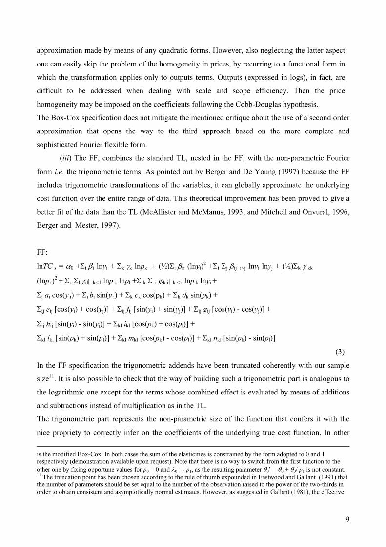
(iii) The FF, combines the standard TL, nested in the FF, with the non-parametric Fourier
form i.e. the trigonometric terms. As pointed out by Berger and De Young (1997) because the FF
includes trigonometric transformations of the variables, it can globally approximate the underlying
cost function over the entire range of data. This theoretical improvement has been proved to give a
better fit of the data than the TL (McAllister and McManus, 1993; and Mitchell and Onvural, 1996,
Berger and Mester, 1997).
FF:
lnTC s = α0 +Σi βi lnyi + Σk γk lnpk + (½)Σi βii (lnyi)2 +Σi Σj βiji<j lnyi lnyj + (½)Σk γ kk
(lnpk)2 + Σk Σl γkl k< l lnp k lnpl +Σ k Σ i ϕk i k < i lnp k lnyi +
Σi ai cos(y i) + Σi bi sin(y i) + Σk ck cos(pk) + Σk dk sin(pk) +
Σij eij [cos(yi) + cos(yj)] + Σij fij [sin(yi) + sin(yj)] + Σij gij [cos(yi) - cos(yj)] +
Σij hij [sin(yi) - sin(yj)] + Σkl ikl [cos(pk) + cos(pl)] +
Σkl lkl [sin(pk) + sin(pl)] + Σkl mkl [cos(pk) - cos(pl)] + Σkl nkl [sin(pk) - sin(pl)]
(3)
In the FF specification the trigonometric addends have been truncated coherently with our sample
size11. It is also possible to check that the way of building such a trigonometric part is analogous to
the logarithmic one except for the terms whose combined effect is evaluated by means of additions
and subtractions instead of multiplication as in the TL.
The trigonometric part represents the non-parametric size of the function that confers it with the
nice propriety to correctly infer on the coefficients of the underlying true cost function. In other
is the modified Box-Cox. In both cases the sum of the elasticities is constrained by the form adopted to 0 and 1 respectively (demonstration available upon request). Note that there is no way to switch from the first function to the other one by fixing opportune values for p0 = 0 and λ0 =- p1, as the resulting parameter θ0’ = θ0 + θ0/ p1 is not constant. 11 The truncation point has been chosen according to the rule of thumb expounded in Eastwood and Gallant (1991) that the number of parameters should be set equal to the number of the observation raised to the power of the two-thirds in order to obtain consistent and asymptotically normal estimates. However, as suggested in Gallant (1981), the effective

10
words the use of the FF confers a substantial gain to the analysis for the fact that it minimizes the
distance from the true function in the Sobolev sense. This allows our analysis the possibility to
work with asymptotically correct nominal sizes of the rejection region for statistical tests (Gallant,
1982) and enables us to estimate the true function with an average prediction bias arbitrarily small
as the number of terms in the Fourier expansion increases (Gallant, 1981). Such a fact attributes a
sort of non parametric property to this flexible functional form, that is not present in the other two
functions considered (TL and Box-Cox). Moreover, special care must be addressed to the choice of
the rescaling form for the trigonometric terms in order to coherently fix their argument in the 0-2π
range. The choice here has fallen on the simple criterion of the ratio to the sample mean as
suggested in Mitchell and Onvural (1996) after having verified the pertinence with the mentioned
interval. Given the local approximation set up of the Box-Cox and TL the corresponding results
must be assessed with particular care for the possible bias in the indicators derived.
It goes without saying that restrictions imposed on TL also hold for the other functional forms.
3.2 The measurement of efficiency
Following Berger (1993) we employ here the distribution-free model for computing the cost
efficiency levels12. The advantage of this model is that it avoids the strong distributional
assumptions of stochastic frontier13. According to this approach the distribution free inefficiency is
based on the distance between the estimated cost function and the s-th effective bank cost in the
sample (s=1,.....,N), assuming that over time the random part of the error term is negligible with
only the error term caused by inefficiency remaining. Hence a straightforward measure of
inefficiency can be denoted as:
inefficiency = exp(min(lnus)-lnus)) (4)
where us is the residual vector after having averaged over time and min(lnus) is the least inefficient
bank in the sample.
3.3 Scale and scope economies
In order to measure how changes in bank output affect cost we use the three estimated cost
equations to construct indicators of scale and scope economies. We use the well-known measures:
number of the coefficients is corrected by reducing the number of the regressors to cope with the possible multicollinearity. 12 For discussion on this approach see Allen and Rai (1996), Ashton (1998), Baltagi (1995), De Young (1997), Drake and Weyman-Jones (1996). 13 See Aigner et. al. (1977), Bauer (1990), Berger (1993), Battese and Coelli (1995).
11
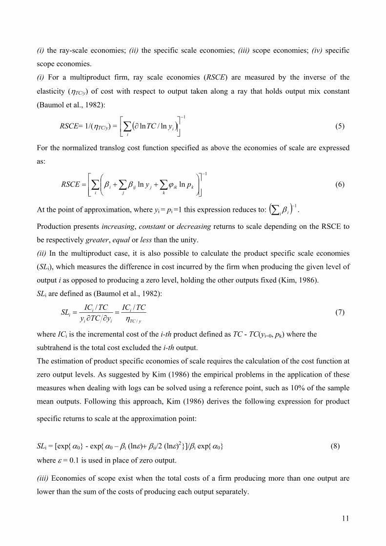
(i) the ray-scale economies; (ii) the specific scale economies; (iii) scope economies; (iv) specific
scope economies.
(i) For a multiproduct firm, ray scale economies (RSCE) are measured by the inverse of the
elasticity (ηTC/y) of cost with respect to output taken along a ray that holds output mix constant
(Baumol et al., 1982):
RSCE= 1/(ηTC/y) = ( )1
ln/ln−
∂∑
iiyTC (5)
For the normalized translog cost function specified as above the economies of scale are expressed
as: 1
lnln−
++= ∑ ∑ ∑
i jk
kikjiji pyRSCE ϕββ (6)
At the point of approximation, where yi = pi =1 this expression reduces to: ( ) 1−∑i iβ .
Production presents increasing, constant or decreasing returns to scale depending on the RSCE to
be respectively greater, equal or less than the unity.
(ii) In the multiproduct case, it is also possible to calculate the product specific scale economies
(SLi), which measures the difference in cost incurred by the firm when producing the given level of
output i as opposed to producing a zero level, holding the other outputs fixed (Kim, 1986).
SLi are defined as (Baumol et al., 1982):
yTC
i
ii
ii
TCICyTCy
TCICSL/
//η
=∂∂
= (7)
where ICi is the incremental cost of the i-th product defined as TC - TC(yi=0, pk) where the
subtrahend is the total cost excluded the i-th output.
The estimation of product specific economies of scale requires the calculation of the cost function at
zero output levels. As suggested by Kim (1986) the empirical problems in the application of these
measures when dealing with logs can be solved using a reference point, such as 10% of the sample
mean outputs. Following this approach, Kim (1986) derives the following expression for product
specific returns to scale at the approximation point:
SLi = [exp{α0} - exp{α0 – βi (lnε)+ βii/2 (lnε)2}]/βi exp{α0} (8)
where ε = 0.1 is used in place of zero output. (iii) Economies of scope exist when the total costs of a firm producing more than one output are
lower than the sum of the costs of producing each output separately.
12
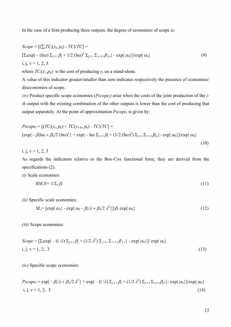
In the case of a firm producing three outputs, the degree of economies of scope is:
Scope = [(∑iTCi(yi, pk) - TC)/TC] =
[Σiexp{– (lnε) Σj ≠ i βj + 1/2 (lnε)2 Σj ≠ i Σ v ≠ i β jv} - exp{α0}]/exp{α0} (9)
i, j, v = 1, 2, 3
where TCi(yi ,pk) is the cost of producing yi on a stand-alone.
A value of this indicator greater/smaller than zero indicates respectively the presence of economies/
diseconomies of scope.
(iv) Product specific scope economies (Pscopei) arise when the costs of the joint production of the i-
th output with the existing combination of the other outputs is lower than the cost of producing that
output separately. At the point of approximation Pscopei is given by:
Pscopei = [(TCi(yi, pk) + TC(yi=0, pk) - TC)/TC] =
[exp{– βilnε + βii/2 (lnε)2} + exp{– lnε Σj ≠ i βj + (1/2 (lnε)2) Σj ≠ i Σv ≠ i βjv}- exp{α0}]/exp{α0}
(10)
i, j, v = 1, 2, 3
As regards the indicators relative to the Box-Cox functional form, they are derived from the
specifications (2).
(i) Scale economies:
RSCE= 1/Σi βi (11)
(ii) Specific scale economies:
SLi= [exp{α0} - exp{α0 – βi/λ + βii/2 λ2}]/βi exp{α0} (12)
(iii) Scope economies:
Scope = [Σiexp{– (1/λ) Σj ≠ i βj + (1/2 λ2) Σ j ≠ i Σ v ≠ i β j v} - exp{α0}]/ exp{α0}
i, j, v = 1, 2, 3 (13)
(iv) Specific scope economies:
Pscopei = exp{– βi/λ + βii/2 λ2} + exp{– (1/λ) Σj ≠ i βj + (1/2 λ2) Σj ≠ i Σv ≠ i βjv}- exp{α0}]/exp{α0}
i, j, v = 1, 2, 3 (14)
13
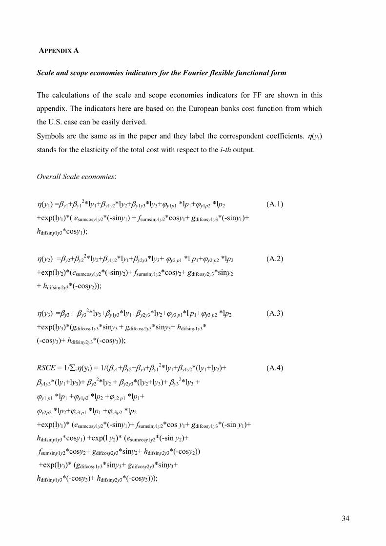
Given the length of the presentation for the FF scale and scope indicators we refer to Appendix A.
In the case of FF scale and scope analysis only the out of the mean sample indicators are reported,
in view of the robustness of the FF on the entire range of data (Gallant, 1981).
4. Empirical findings
In our empirical analysis we present the evidence from the TL, FF and Box-Cox cost function
specifications both for European and for U.S. commercial banks.
In the case of European banks we run a common frontier. This analysis, on the one hand, allows to
compare performances of banks across countries. On the other hand, it does not allow to determine
whether divergence in inefficiency is due to differences in the technology used or to environmental
conditions14. We face the latter criticism using only one type of financial institution: the commercial
banks. For these banks the assumption of employing the same technology could be supported by
considering that commercial banks provide all over Europe the same financial services and
activities. Moreover, we employ dummies for each of the 15 European countries in order to capture
differences across countries.
4.1 Cost functions estimations
In this section we present both the results of the cost functions estimations for European and U.S.
commercial banks.
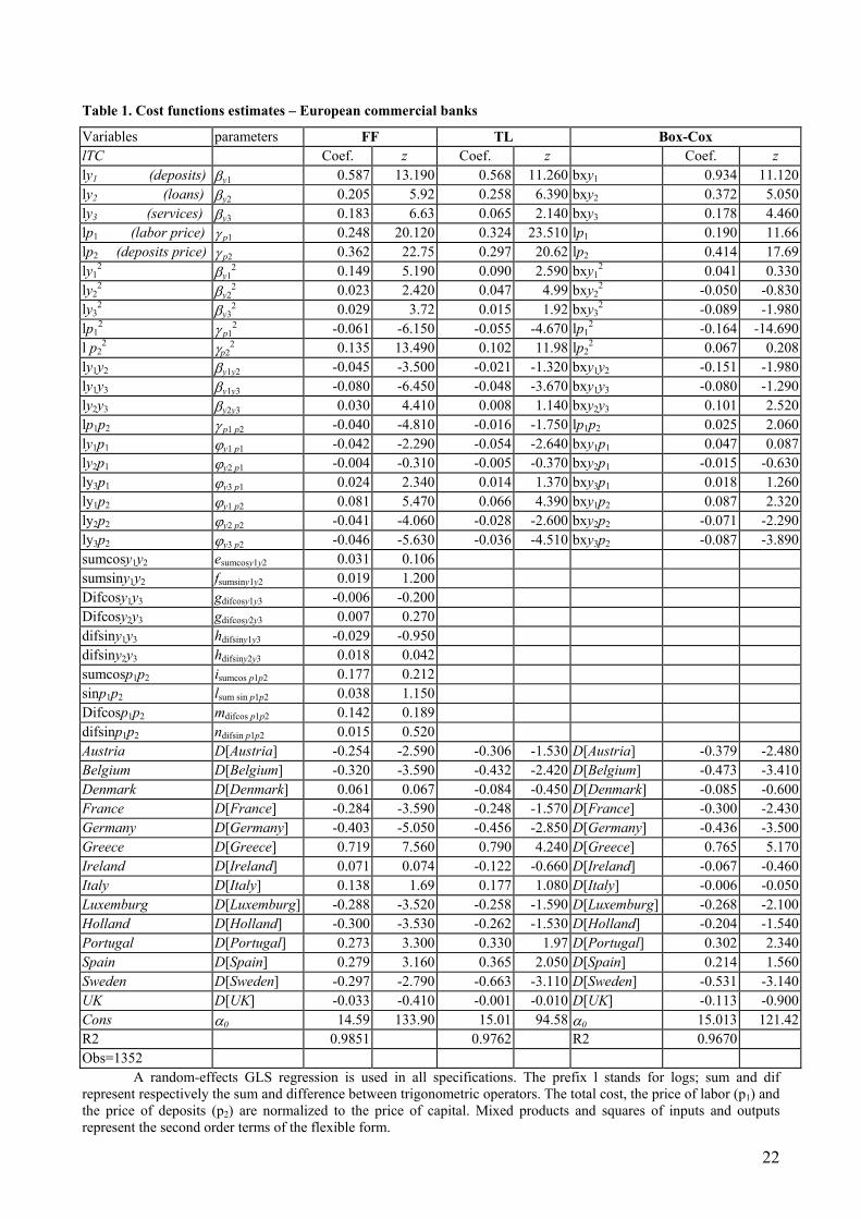
In Table 1 we show the evidence from the FF, TL and Box-Cox specifications for European banks.
Overall the results obtained are consistent over the different specifications used.
As regards the TL estimations we can point out the following results.
[insert Table 1]
1) It is noteworthy that all the outputs and input price coefficients present the expected
positive sign and are significant.
2) The elasticities of production costs to unit staff (γp1=0.324) and to deposit price
(γp2=0.297) are smaller than the elasticity to the capital price (0.379= 1-γp1-γp2) for the linear
homogeneity conditions imposed on the TL cost function. This means that banks can control more
personnel and deposit expenses than capital expenses when prices rise. A plausible explanation is
that, at least in the short run, it seems more difficult to cut capital expenses, especially in the field of
14 To account for these effects, Dietsch and Lozano Vivas (2000) impose a cross-equation equality restriction on the parameters of each country’s cost frontier in order to obtain results which are not influenced by the country’s
14
information technology, less so far labor costs. Similar evidence has been found by Resti (1997) for
a sample of Italian banks and is quite consistent with the ongoing tendency in Europe of
restructuring.
The elasticity to deposit price shows the importance of interest on deposits in the European market.
Moreover, the positive and significant deposits price coefficient supports the choice of considering
such price as an input.
3) Among outputs, deposits (βy1= 0.568) are more cost absorbing than loans and services.
This result at a first look could appear surprising if one considers that the lending activity is
expected to be more cost absorbing than the deposit management, because of high costs connected
with the monitoring and collection of non performing loans. However, as pointed out also by Resti
(1997), who found the same evidence on a sample of Italian banks, deposits may imply a larger
network of branches which in turn increases operating costs.
As we expected, services are the least cost absorbing output (βy3= 0.065) since they are less
dependent on the firm’s physical capital. Moreover, they have not been the most important source
of income for banks in Europe. The sharp reduction of the bank’s main profit source (interest
income), which has occurred in the last few years, is forcing banks to find new income alternatives
to deal in. In this respect, services may become one of the non-interest income sources, thus
implying a larger impact on the cost function.
As far as the FF and Box-Cox are concerned we find some small differences when compared with
TL estimates. The result that deposits are the most cost absorbing output is largely confirmed (0.587
for FF and 0.934 for Box-Cox). Moreover there is also clear evidence on services (0.183 for FF and
0.178 for Box-Cox) which result to be the least cost absorbing output with respect to loans (0.205
for FF and 0.372 for Box-Cox) and deposits.
The coefficients for deposits and loans are largely overvalued with the Box-Cox specification when
compared with the TL and the FF specifications. The FF and the Box-Cox provide almost the same
elasticity for services, which is significantly higher than that obtained with the TL.
Considering the input prices, both the FF and the Box-Cox estimates produce lower elasticity
coefficients for capital price (0.248 for FF and 0.19 for the Box-Cox).
Finally, the common evidence across the three cost function specifications is that deposits are the
most cost absorbing output and services the least cost absorbing one; among the input prices, capital
shows the highest elasticity.
technology. They add country-specific environmental variables to the cost function specification to measure the impact of those variables on the differences among country inefficiencies.
15
This evidence describes European commercial banks as characterized by high cost elasticity to
deposits which pay high interest rates and increase operative costs associated with the network of
branches.
4) As far as the countries effect is concerned the UK, Denmark and Ireland lay on the
European average15. We find that the FF specification supports fixed effects better than the other
two functional forms.
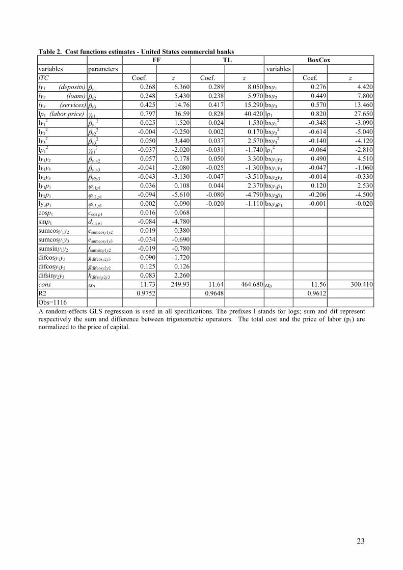
Table 2 presents the evidence for the U.S. commercial banks obtained from the three different
functional form estimates. As pointed out above (par. 2.2), in the case of U.S. commercial banks we
model the cost functions following the value added approach. The choice of adopting a different
cost function - in which we do not include the price of deposits among the inputs - is supported by
the test on the specification, and by the fact that the cost of deposits for U.S. banks is quite
negligible.
[insert Table 2]
In the case of U.S. commercial banks the evidence provided by our analysis seems quite consistent
across the different specifications employed: coefficients present almost the same values, and are
strongly significant. Only the Box-Cox estimates for loans and services tend to be slightly
overvalued compared to the TL and FF figures. Overall, the evidence suggests considering results
reliable.
As expected the outcome underlines a large difference between European and U.S. commercial
banks.
As opposed to the European case, in all specifications the most cost absorbing output is services,
with the elasticity for deposits and loans always lower.
The level and the quality of services provided to customers, more than deposits, have been an
important source of income for U.S. commercial banks. Therefore it seems plausible to expect
higher cost connected to the production of this item, which requires high investment in financial
system technology (software, telecommunication, etc.) and human capital.
Looking at the input prices, surprisingly and contrarily to what one might expect, given also the
flexibility of the labor market, the elasticity of production cost to unit staff is much higher than the
elasticity to capital price. Such a result has also been confirmed by the other two functional forms.
This evidence would imply that firms can control more easily capital, cutting down its demand,
rather than labor, when prices rise.
The puzzling evidence has to be addressed with caution since we are considering a period of
exceptional growth for the U.S. economy (driven also by the new economy and information
15 For these countries the dummies are not significantly different from zero.
16
technology). High profit expectations and growing demand for factors, which characterized the
period, may make constraints less binding16. This is also consistent with the high level of
inefficiency obtained from our analysis.
Finally, the analysis for Europe and the U.S. shows that the three functional forms employed
performed quite well producing in most cases consistent evidence. However, tests performed on the
nested TL versus FF functional forms show, tenuous evidence in favor of FF for Europe and a
stronger one for the U.S.17.This empirical outcome finds support in White (1980), Gallant (1981)
and Mitchell and Onvural (1996) which show the superiority of the FF with the respect to TL
estimations.
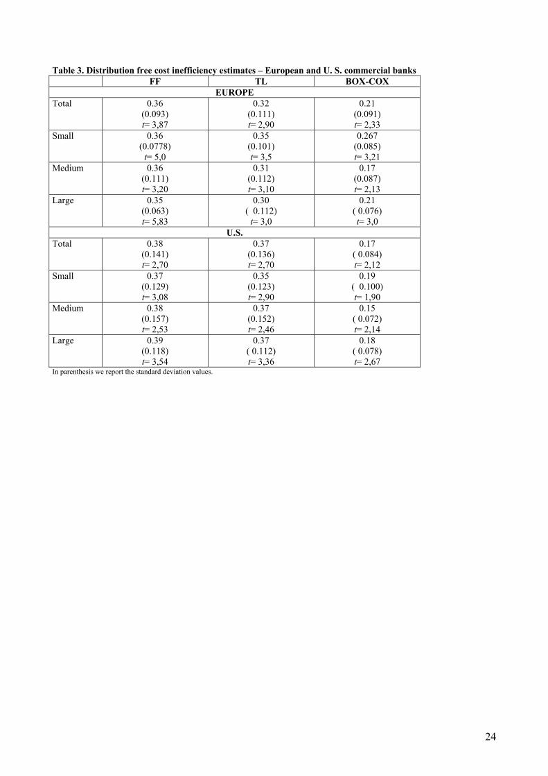
4.2 Distribution free cost efficiency results.
The distribution free cost inefficiency estimates, in Table 3, point out a significant level of
inefficiency both for European and U.S. commercials banks. This evidence is consistent with the
analysis in Bauer (1990), Allen and Rai (1996), Cavallo and Rossi (2001) and Vander-Vennet
(2002), which also find significant level of inefficiency in the banking industry. Moreover, our
results are strengthened by the inefficiency scorers we obtained by using the stochastic frontier
approach18.
While Box-Cox tends to overestimate the efficiency scores, both TL and FF cost functions show
similar outcomes (see Table 3).
[insert Table 3]
For Europe, we find an average inefficiency level of 32 per cent with the TL, 36 per cent with the
FF, and 20 per cent with the Box-Cox specification. While the magnitude of inefficiency dispersion
between TL (reporting a deviation of 0.11 with a minimum of 15 per cent inefficiency) and the FF
(standard deviation of 0.093 and a minimum value of 17 per cent) is quite similar, the distribution
of Box-Cox cost inefficiency shows lower inefficiency levels (20 per cent) with a standard
deviation of 0.091 and a minimum of 6 per cent.
16 This evidence may be also supported by the fact that under fixed term contracts, which are the standard in the flexible structure of the U.S. labour market, workers in financial institutions benefit from large compensation payments if fired. 17 We reject the Ho hypothesis on the base of the Ramsey-Reset test according to which model has no omitted variables at a level of confidence of 5%: Pvalue = 0.010 for Europe, Pvalue = 0.12, for the U.S. 18 Berger and Mester (1997) also find that the efficiency level with the stochastic and the free distribution approach are similar. Our stochastic frontier estimates, obtained by Frontier 4.1 (Coelli, 96), are available upon request.
17
The analysis by bank dimension shows that for both European and U.S. commercial banks there is
not a consistent size effect, as also found by Vander-Vennet (2002) for a sample of European banks.
This evidence shows that our findings are robust over the size samples used19.
In particular, while FF presents almost the same score across sizes, TL and Box-Cox estimates
show that efficiency tends to slightly decrease as the bank size increases. The cost inefficiency
results for U.S. commercial banks suggest that the Box-Cox specification, as in the European case,
overestimates the efficiency scores.
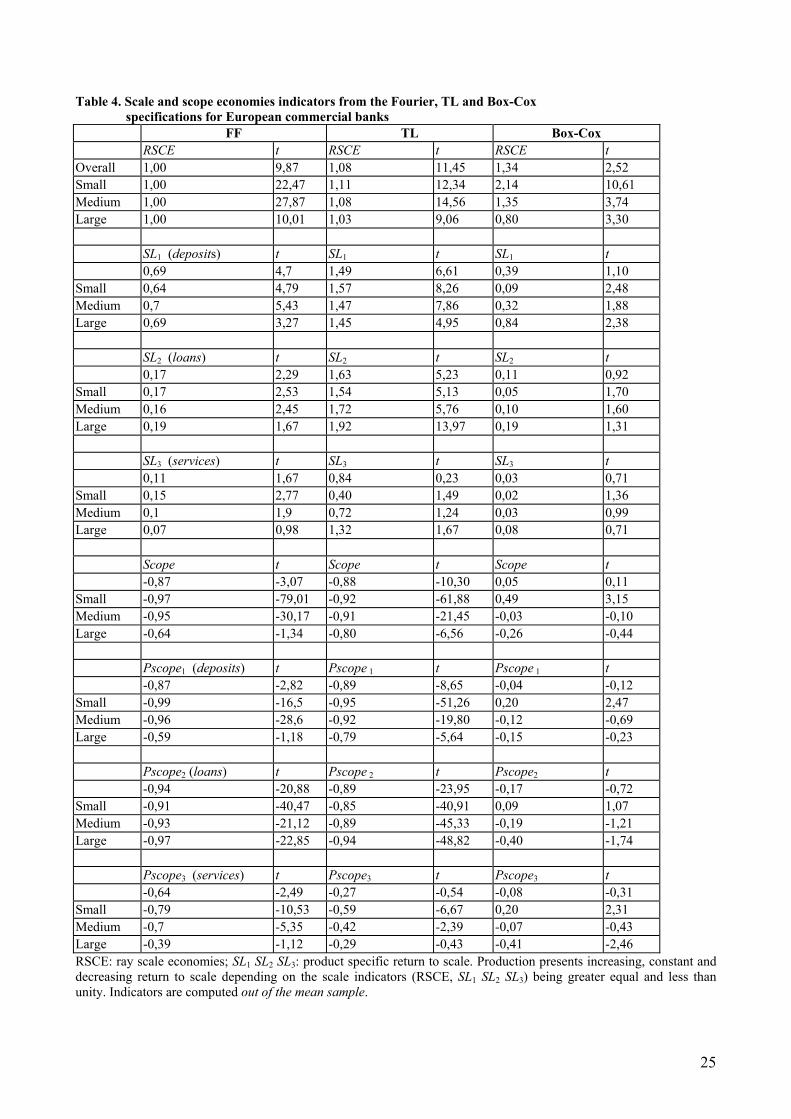
4.3 Scale and scope economies findings
In this section we present the evidence on scale and scope economies indicators obtained from the
different cost functions for European and U.S. commercial banks. The aim here is to provide new
evidence on bank output efficiency by using different functional forms (TL, FF and Box-Cox), and
to check the robustness of the results over the specifications employed.
The estimations are computed both out of the mean sample and at the mean sample. Obviously the
former analysis allows us to infer on the indicators obtained.
The evidence computed out of the mean sample for European Commercial banks (Table 4) can be
summarized as follows.
[insert Table 4]
(i) Constant scale economies (RSCE), product specific diseconomies of scale (SLi),
diseconomies of scope (Scope) and specific scope (Pscopei) diseconomies are detected in
our study20.
(ii) Since the results provided seem to be sensitive to the different functional forms employed,
output efficiency scores should be interpreted with caution. Box-Cox provides evidence in
favor of increasing returns to scale with the exception of large banks. On the contrary, TL
scale economies are roughly constant both overall and at size level as in the FF case.
(iii) Bank size classification - small, medium and large - does not significantly affect scale and
scope economies indicators in the TL and FF. Almost all the scale indicators - both global
and specific - obtained with these two specifications exhibit a quite stable pattern through
the different bank sizes with a slight tendency for loans to increase as the dimension of a
bank becomes larger. On the contrary, the Box-Cox scale economies indicators appear to be
19 As mentioned in par. 2.2, in our analysis we consider data only from large commercial banks. We split the sample in three classes according to the asset size distribution. Consequently, for small banks we mean the smallest in our sample. 20 While some of our results are consistent with Vander-Vennet (2002), different evidence has been provided in Cavallo and Rossi (2001) over a wider tipology of financial institutions for the period 1992-97 in six European countries.
18
sensitive to the bank size, suggesting that the returns to scale are more pronounced for small
banks. Looking at the Box-Cox product specific scale indicators the production of deposits
seems to generate smaller diseconomies of scale as the size of the bank increases.
(iv) Product specific diseconomies of scales are detected in all the specifications, with the
exception of deposits and loans in the TL specification.
(v) Diseconomies of scope are obtained by all functional forms. The presence of negative scope
economies - lower than one in absolute values - indicates that the joint production of the
three outputs - deposits, loans and services - is inefficient. Looking at the evidence from the
three specifications, in the case of scope indicators the most significant results are those
obtained with FF specification followed by the TL, which appear to fit the data poorly with
respect to services scope economies. The Box-Cox specification seems to produce poorer
scope indicators, although the sign, the magnitude and size effect, are consistent with the
other two specifications. The evidence shows higher absolute values of scope diseconomies
as the size of the firm decreases. This result may suggest that large size banks present less
diseconomies of scope than small banks, suggesting that small financial institutions are less
efficient in the joint multi output production.
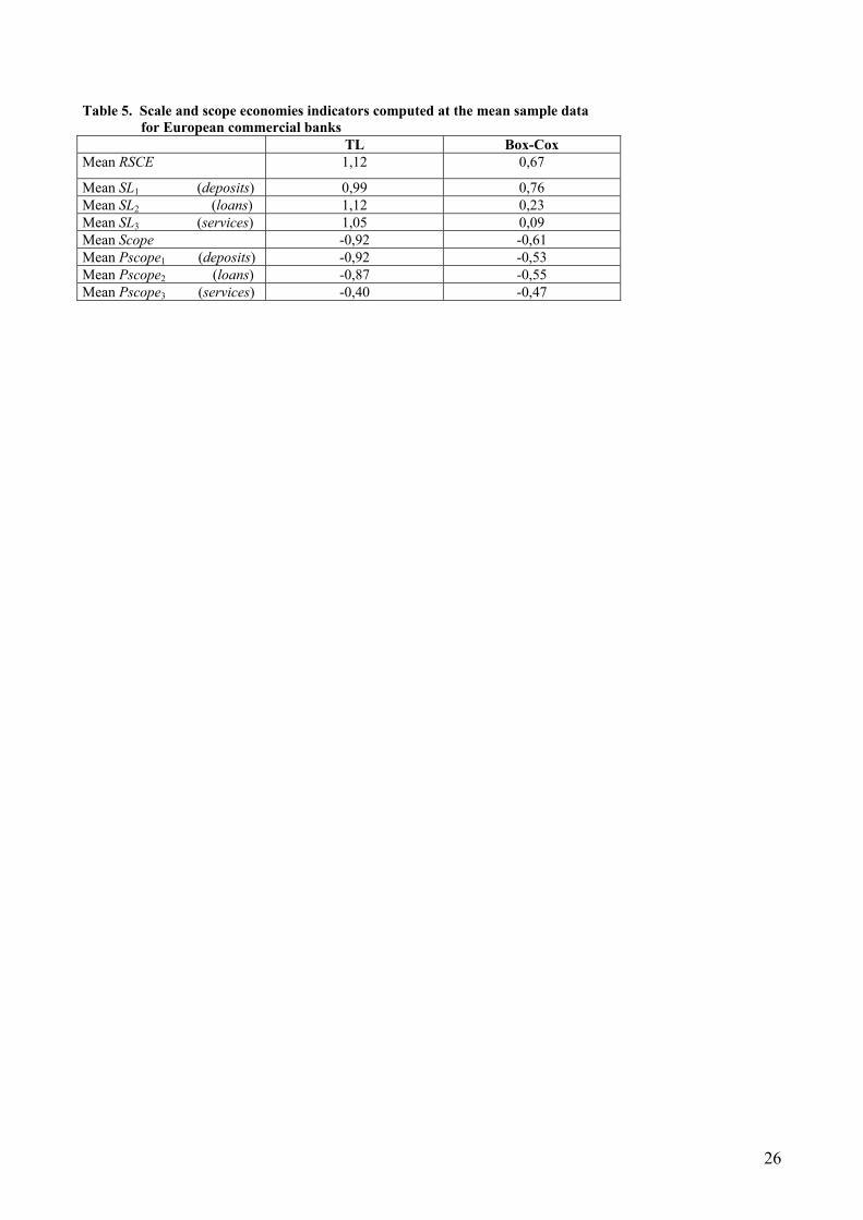
Due to the second order approximation of the TL and the Box-Cox, their fit, in the out of the
mean sample data, may be poorer compared to the FF (Gallant, 1981). Therefore, TL and Box-Cox
scale and scope indicators have also been computed at the mean sample (Table 5).
[insert Table 5]
While TL scale and scope estimates in the approximation point produce consistent evidence with
previous analysis (out of the mean sample), the Box-Cox indicators seem to deviate from the out of
the mean sample results: they undervalue the overall scale economies and slightly overvalue the
scope indicators.
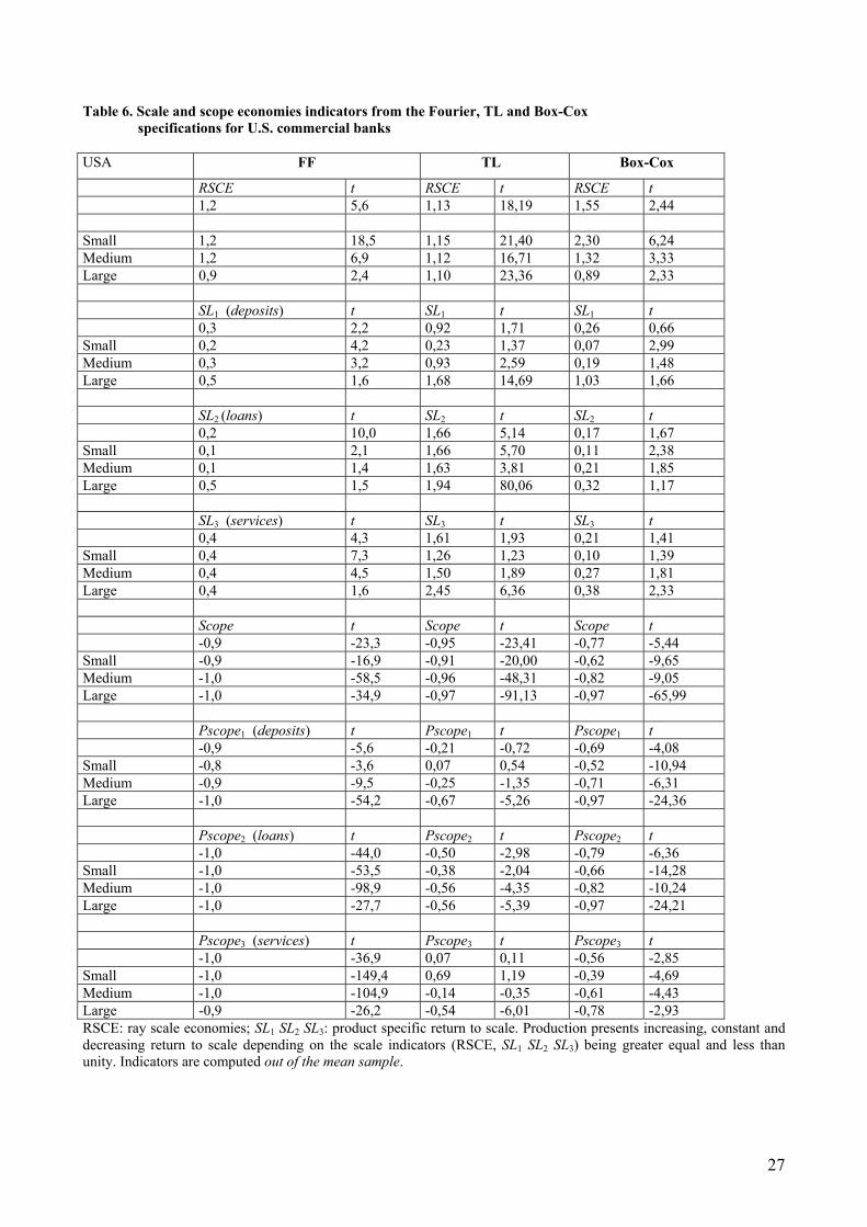
As far as U.S. out of the mean sample indicators are concerned (Table 6), we can summarize the
following evidence.
[insert Table 6]
(i) Results show the presence of overall scale economies, being more pronounced for
small and medium banks. Large banks present slight diseconomies of scale (FF, Box-
Cox) and almost constant return to scale (TL). This evidence may suggest that a
broader firm may incur higher physical capital and innovation costs, which do not
suffice to exploit scale economies, given the U shaped average cost function.
(ii) Product specific diseconomies of scale are detected by the analysis. Only in the case
of the TL estimates we find evidence in favor of increasing specific scale economies
19
for loans and services. Therefore, at the product specific scale economies level, the
most consistent evidence across the different specifications, is the presence of
product specific diseconomies of scale for deposits, which is significantly smaller
than unity (with the exception for large banks which present product specific
increasing economies of scale). This evidence suggests that the production of
deposits, due to the fact that it requires a wide network of branches, may cause a
more than proportional rise in total costs21.
(iii) The tendency of product specific scale indicators to grow with bank size shows that
U.S. large commercial banks, seem to be more efficient or less inefficient in the
production of specific output than in the overall case.
(iv) As far as the scope indicators are concerned, also for U.S. banks we find negative
values of scope economies indicators over the different specifications.
(v) Based on the Ramsey test, which shows that FF for U.S. banks approximates the true
function better than the other functional forms, we tend to rely more upon the FF
scale and scope indicators. Moreover, the indicators obtained from FF present always
higher t values.
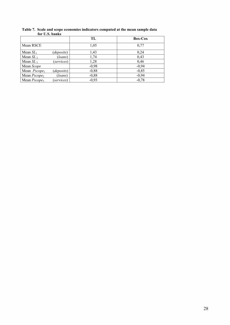
As regards the indicators computed at the mean sample, the evidence almost confirms the
results obtained by the out of the mean sample estimates: for TL, presence of overall constant
returns to scale are detected, and increasing product scale economies are found for the three outputs
(Table 7).
[insert Table 7]
For the Box-Cox estimates we obtain, consistently with previous analysis, specific
diseconomies of scale and, differently from the out of the mean sample estimates, overall
diseconomies of scale. Given the evidence on the overall scale economies, the Box-Cox
approximation point estimates, tend to deviate more than the TL from the out of the mean sample
analysis.
Finally, the evidence from the out of and at the mean sample estimations support the view
that both scale and scope economies, are larger in U.S. than in European banks. An acceptable
reason for this is probably the higher level of technology included in the productive structure of
U.S. banks, as shown in Hunter and Timme (1991), and the restructuring process occurred
previously than in Europe.
5. Conclusions
21 Note that this result does not contradict the low elasticity values for deposits, as specific economies of scale
20
The econometric analysis performed through the different specifications enables us to reach
some conclusions regarding the cost structure of U.S. and European commercial banks.
The use of the Fourier, translog and Box-Cox functions helped us in evaluating the robustness of
our results through the several specifications proposed. Although the evidence on the cost function
parameters presents some consistent values over the different functional forms, tests performed on
the specifications are in favor of the Fourier which, turns up to better fit our data.
Results for the two banking systems are coherent with the evidence that European commercial
banks are traditionally more oriented to deposits and retails, while U.S. commercial banks are also
focused on the services, given also the impact of the innovation in the field of information
technology.
Consistently we find for Europe that deposits are the most cost absorbing output, since they may
require a broad network of branches which causes an increase in costs. On the contrary, services
turn out to be the least cost absorbing output as they traditionally had never been the core bank
activity in Europe.
For U.S. commercial banks services are found to be the most cost absorbing output, since they may
involve high investments in information technology and human capital.
As far as the input prices are concerned, European commercial banks turn out to control more
personnel and deposits expenses than capital when prices rise. This evidence is quite consistent with
the ongoing tendency in Europe to restructuring through mergers and acquisitions. The need for
restructuring is also consistent with significant level of inefficiency detected by the cost efficiency
estimates.
Looking at the input prices for U.S. commercial banks, surprisingly and contrarily to what one
might expect, production costs are more sensitive to unit staff than to capital price. This evidence
would imply that firms can control more easily capital, cutting down its demand, rather than the
demand for labor, when prices rise.
The puzzling evidence has to be considered with caution since we are looking at a period (1995-
1998) of exceptional growth and low levels of unemployment for the U.S. economy. High profit
expectations and the consequent growing demand for labor, which characterized the period, may
make constraints less binding. This also turns out to be consistent with the high level of inefficiency
obtained from our analysis.
Looking at scale economies indicators, we find increasing global scale economies for the U.S. and
less pronounced evidence for Europe. This may be due to the higher information technology
indicators are based on the definition of incremental cost which is posed in discrete sense.
21
embedded in the production function of U.S. banks which obviously has an impact on the
productivity of the system.
The findings for scale economies in Europe, however have to be interpreted with caution, since
indicators obtained seem to be sensitive to the different functional forms employed. Box-Cox
provides evidence in favor of increasing return to scale economies with the exception of large
banks. On the contrary, TL scale economies are roughly constant both overall and at size level as in
the FF case.
As far as the scope indicators are concerned we find evidence of diseconomies of scope, detected by
all the functional forms, both in Europe and in the U.S. Such evidence, which is consistent with the
significant level of inefficiency detected, is likely to be associated to the consolidation process for
Europe and to the less binding constraints for U.S., given the positive expectations and the high
pace growth during the period considered.
22
Table 1. Cost functions estimates – European commercial banks
Variables parameters FF TL Box-Cox lTC Coef. z Coef. z Coef. z ly1 (deposits) βy1 0.587 13.190 0.568 11.260 bxy1 0.934 11.120ly2 (loans) βy2 0.205 5.92 0.258 6.390 bxy2 0.372 5.050ly3 (services) βy3 0.183 6.63 0.065 2.140 bxy3 0.178 4.460lp1 (labor price) γ p1 0.248 20.120 0.324 23.510 lp1 0.190 11.66lp2 (deposits price) γ p2 0.362 22.75 0.297 20.62 lp2 0.414 17.69ly1
2 βy12 0.149 5.190 0.090 2.590 bxy1
2 0.041 0.330ly2
2 βy22 0.023 2.420 0.047 4.99 bxy2
2 -0.050 -0.830ly3
2 βy32 0.029 3.72 0.015 1.92 bxy3
2 -0.089 -1.980lp1
2 γ p12 -0.061 -6.150 -0.055 -4.670 lp1
2 -0.164 -14.690l p2
2 γp22 0.135 13.490 0.102 11.98 lp2
2 0.067 0.208ly1y2 βy1y2 -0.045 -3.500 -0.021 -1.320 bxy1y2 -0.151 -1.980ly1y3 βy1y3 -0.080 -6.450 -0.048 -3.670 bxy1y3 -0.080 -1.290ly2y3 βy2y3 0.030 4.410 0.008 1.140 bxy2y3 0.101 2.520lp1p2 γ p1 p2 -0.040 -4.810 -0.016 -1.750 lp1p2 0.025 2.060ly1p1 ϕy1 p1 -0.042 -2.290 -0.054 -2.640 bxy1p1 0.047 0.087ly2p1 ϕy2 p1 -0.004 -0.310 -0.005 -0.370 bxy2p1 -0.015 -0.630ly3p1 ϕy3 p1 0.024 2.340 0.014 1.370 bxy3p1 0.018 1.260ly1p2 ϕy1 p2 0.081 5.470 0.066 4.390 bxy1p2 0.087 2.320ly2p2 ϕy2 p2 -0.041 -4.060 -0.028 -2.600 bxy2p2 -0.071 -2.290ly3p2 ϕy3 p2 -0.046 -5.630 -0.036 -4.510 bxy3p2 -0.087 -3.890sumcosy1y2 esumcosy1y2 0.031 0.106 sumsiny1y2 fsumsiny1y2 0.019 1.200 Difcosy1y3 gdifcosy1y3 -0.006 -0.200 Difcosy2y3 gdifcosy2y3 0.007 0.270 difsiny1y3 hdifsiny1y3 -0.029 -0.950 difsiny2y3 hdifsiny2y3 0.018 0.042 sumcosp1p2 isumcos p1p2 0.177 0.212 sinp1p2 lsum sin p1p2 0.038 1.150 Difcosp1p2 mdifcos p1p2 0.142 0.189 difsinp1p2 ndifsin p1p2 0.015 0.520 Austria D[Austria] -0.254 -2.590 -0.306 -1.530 D[Austria] -0.379 -2.480Belgium D[Belgium] -0.320 -3.590 -0.432 -2.420 D[Belgium] -0.473 -3.410Denmark D[Denmark] 0.061 0.067 -0.084 -0.450 D[Denmark] -0.085 -0.600France D[France] -0.284 -3.590 -0.248 -1.570 D[France] -0.300 -2.430Germany D[Germany] -0.403 -5.050 -0.456 -2.850 D[Germany] -0.436 -3.500Greece D[Greece] 0.719 7.560 0.790 4.240 D[Greece] 0.765 5.170Ireland D[Ireland] 0.071 0.074 -0.122 -0.660 D[Ireland] -0.067 -0.460Italy D[Italy] 0.138 1.69 0.177 1.080 D[Italy] -0.006 -0.050Luxemburg D[Luxemburg] -0.288 -3.520 -0.258 -1.590 D[Luxemburg] -0.268 -2.100Holland D[Holland] -0.300 -3.530 -0.262 -1.530 D[Holland] -0.204 -1.540Portugal D[Portugal] 0.273 3.300 0.330 1.97 D[Portugal] 0.302 2.340Spain D[Spain] 0.279 3.160 0.365 2.050 D[Spain] 0.214 1.560Sweden D[Sweden] -0.297 -2.790 -0.663 -3.110 D[Sweden] -0.531 -3.140UK D[UK] -0.033 -0.410 -0.001 -0.010 D[UK] -0.113 -0.900Cons α0 14.59 133.90 15.01 94.58 α0 15.013 121.42R2 0.9851 0.9762 R2 0.9670Obs=1352
A random-effects GLS regression is used in all specifications. The prefix l stands for logs; sum and dif represent respectively the sum and difference between trigonometric operators. The total cost, the price of labor (p1) and the price of deposits (p2) are normalized to the price of capital. Mixed products and squares of inputs and outputs represent the second order terms of the flexible form.
23
Table 2. Cost functions estimates - United States commercial banks FF TL BoxCox variables parameters variables lTC Coef. z Coef. z Coef. z ly1 (deposits) βy1 0.268 6.360 0.289 8.050 bxy1 0.276 4.420ly2 (loans) βy2 0.248 5.430 0.238 5.970 bxy2 0.449 7.800ly3 (services) βy3 0.425 14.76 0.417 15.290 bxy3 0.570 13.460lp1 (labor price) γp1 0.797 36.59 0.828 40.420 lp1 0.820 27.650ly1
2 βy12 0.025 1.520 0.024 1.530 bxy1
2 -0.348 -3.090ly2
2 βy22 -0.004 -0.250 0.002 0.170 bxy2
2 -0.614 -5.040ly3
2 βy32 0.050 3.440 0.037 2.570 bxy3
2 -0.140 -4.120lp1
2 γp12 -0.037 -2.020 -0.031 -1.740 lp1
2 -0.064 -2.810ly1y2 βy1y2 0.057 0.178 0.050 3.300 bxy1y2 0.490 4.510ly1y3 βy1y3 -0.041 -2.080 -0.025 -1.300 bxy1y3 -0.047 -1.060ly2y3 βy2y3 -0.043 -3.130 -0.047 -3.510 bxy2y3 -0.014 -0.330ly1p1 ϕy1p1 0.036 0.108 0.044 2.370 bxy1p1 0.120 2.530ly2p1 ϕy2 p1 -0.094 -5.610 -0.080 -4.790 bxy2p1 -0.206 -4.500ly3p1 ϕy3 p1 0.002 0.090 -0.020 -1.110 bxy3p1 -0.001 -0.020cosp1 ccos p1 0.016 0.068 sinp1 dsin p1 -0.084 -4.780 sumcosy1y2 esumcosy1y2 0.019 0.380 sumcosy1y3 esumcosy1y3 -0.034 -0.690 sumsiny1y2 fsumsiny1y2 -0.019 -0.780 difcosy1y3 gdifcosy2y3 -0.090 -1.720 difcosy1y2 gdifcosy2y2 0.125 0.126 difsiny2y3 hdifsiny2y3 0.083 2.260 cons α0 11.73 249.93 11.64 464.680 α0 11.56 300.410R2 0.9752 0.9648 0.9612 Obs=1116 A random-effects GLS regression is used in all specifications. The prefixes l stands for logs; sum and dif represent respectively the sum and difference between trigonometric operators. The total cost and the price of labor (p1) are normalized to the price of capital.
24
Table 3. Distribution free cost inefficiency estimates – European and U. S. commercial banks FF TL BOX-COX
EUROPE Total
0.36 (0.093) t= 3,87
0.32 (0.111) t= 2,90
0.21 (0.091) t= 2,33
Small 0.36 (0.0778)
t= 5,0
0.35 (0.101) t= 3,5
0.267 (0.085) t= 3,21
Medium
0.36 (0.111) t= 3,20
0.31 (0.112) t= 3,10
0.17 (0.087) t= 2,13
Large 0.35 (0.063) t= 5,83
0.30 ( 0.112)
t= 3,0
0.21 ( 0.076) t= 3,0
U.S. Total 0.38
(0.141) t= 2,70
0.37 (0.136) t= 2,70
0.17 ( 0.084) t= 2,12
Small 0.37 (0.129) t= 3,08
0.35 (0.123) t= 2,90
0.19 ( 0.100) t= 1,90
Medium 0.38 (0.157) t= 2,53
0.37 (0.152) t= 2,46
0.15 ( 0.072) t= 2,14
Large 0.39 (0.118) t= 3,54
0.37 ( 0.112) t= 3,36
0.18 ( 0.078) t= 2,67
In parenthesis we report the standard deviation values.
25
Table 4. Scale and scope economies indicators from the Fourier, TL and Box-Cox specifications for European commercial banks
FF TL Box-Cox RSCE t RSCE t RSCE t
Overall 1,00 9,87 1,08 11,45 1,34 2,52 Small 1,00 22,47 1,11 12,34 2,14 10,61 Medium 1,00 27,87 1,08 14,56 1,35 3,74 Large 1,00 10,01 1,03 9,06 0,80 3,30
SL1 (deposits) t SL1 t SL1 t 0,69 4,7 1,49 6,61 0,39 1,10
Small 0,64 4,79 1,57 8,26 0,09 2,48 Medium 0,7 5,43 1,47 7,86 0,32 1,88 Large 0,69 3,27 1,45 4,95 0,84 2,38
SL2 (loans) t SL2 t SL2 t 0,17 2,29 1,63 5,23 0,11 0,92
Small 0,17 2,53 1,54 5,13 0,05 1,70 Medium 0,16 2,45 1,72 5,76 0,10 1,60 Large 0,19 1,67 1,92 13,97 0,19 1,31
SL3 (services) t SL3 t SL3 t 0,11 1,67 0,84 0,23 0,03 0,71
Small 0,15 2,77 0,40 1,49 0,02 1,36 Medium 0,1 1,9 0,72 1,24 0,03 0,99 Large 0,07 0,98 1,32 1,67 0,08 0,71
Scope t Scope t Scope t -0,87 -3,07 -0,88 -10,30 0,05 0,11
Small -0,97 -79,01 -0,92 -61,88 0,49 3,15 Medium -0,95 -30,17 -0,91 -21,45 -0,03 -0,10 Large -0,64 -1,34 -0,80 -6,56 -0,26 -0,44
Pscope1 (deposits) t Pscope 1 t Pscope 1 t -0,87 -2,82 -0,89 -8,65 -0,04 -0,12
Small -0,99 -16,5 -0,95 -51,26 0,20 2,47 Medium -0,96 -28,6 -0,92 -19,80 -0,12 -0,69 Large -0,59 -1,18 -0,79 -5,64 -0,15 -0,23
Pscope2 (loans) t Pscope 2 t Pscope2 t -0,94 -20,88 -0,89 -23,95 -0,17 -0,72
Small -0,91 -40,47 -0,85 -40,91 0,09 1,07 Medium -0,93 -21,12 -0,89 -45,33 -0,19 -1,21 Large -0,97 -22,85 -0,94 -48,82 -0,40 -1,74
Pscope3 (services) t Pscope3 t Pscope3 t -0,64 -2,49 -0,27 -0,54 -0,08 -0,31
Small -0,79 -10,53 -0,59 -6,67 0,20 2,31 Medium -0,7 -5,35 -0,42 -2,39 -0,07 -0,43 Large -0,39 -1,12 -0,29 -0,43 -0,41 -2,46 RSCE: ray scale economies; SL1 SL2 SL3: product specific return to scale. Production presents increasing, constant and decreasing return to scale depending on the scale indicators (RSCE, SL1 SL2 SL3) being greater equal and less than unity. Indicators are computed out of the mean sample.
26
Table 5. Scale and scope economies indicators computed at the mean sample data for European commercial banks
TL Box-Cox Mean RSCE 1,12 0,67
Mean SL1 (deposits) 0,99 0,76 Mean SL2 (loans) 1,12 0,23 Mean SL3 (services) 1,05 0,09 Mean Scope -0,92 -0,61 Mean Pscope1 (deposits) -0,92 -0,53 Mean Pscope2 (loans) -0,87 -0,55 Mean Pscope3 (services) -0,40 -0,47
27
Table 6. Scale and scope economies indicators from the Fourier, TL and Box-Cox specifications for U.S. commercial banks
USA FF TL Box-Cox
RSCE t RSCE t RSCE t 1,2 5,6 1,13 18,19 1,55 2,44 Small 1,2 18,5 1,15 21,40 2,30 6,24 Medium 1,2 6,9 1,12 16,71 1,32 3,33 Large 0,9 2,4 1,10 23,36 0,89 2,33 SL1 (deposits) t SL1 t SL1 t 0,3 2,2 0,92 1,71 0,26 0,66 Small 0,2 4,2 0,23 1,37 0,07 2,99 Medium 0,3 3,2 0,93 2,59 0,19 1,48 Large 0,5 1,6 1,68 14,69 1,03 1,66 SL2 (loans) t SL2 t SL2 t 0,2 10,0 1,66 5,14 0,17 1,67 Small 0,1 2,1 1,66 5,70 0,11 2,38 Medium 0,1 1,4 1,63 3,81 0,21 1,85 Large 0,5 1,5 1,94 80,06 0,32 1,17 SL3 (services) t SL3 t SL3 t 0,4 4,3 1,61 1,93 0,21 1,41 Small 0,4 7,3 1,26 1,23 0,10 1,39 Medium 0,4 4,5 1,50 1,89 0,27 1,81 Large 0,4 1,6 2,45 6,36 0,38 2,33 Scope t Scope t Scope t -0,9 -23,3 -0,95 -23,41 -0,77 -5,44 Small -0,9 -16,9 -0,91 -20,00 -0,62 -9,65 Medium -1,0 -58,5 -0,96 -48,31 -0,82 -9,05 Large -1,0 -34,9 -0,97 -91,13 -0,97 -65,99 Pscope1 (deposits) t Pscope1 t Pscope1 t -0,9 -5,6 -0,21 -0,72 -0,69 -4,08 Small -0,8 -3,6 0,07 0,54 -0,52 -10,94 Medium -0,9 -9,5 -0,25 -1,35 -0,71 -6,31 Large -1,0 -54,2 -0,67 -5,26 -0,97 -24,36 Pscope2 (loans) t Pscope2 t Pscope2 t -1,0 -44,0 -0,50 -2,98 -0,79 -6,36 Small -1,0 -53,5 -0,38 -2,04 -0,66 -14,28 Medium -1,0 -98,9 -0,56 -4,35 -0,82 -10,24 Large -1,0 -27,7 -0,56 -5,39 -0,97 -24,21 Pscope3 (services) t Pscope3 t Pscope3 t -1,0 -36,9 0,07 0,11 -0,56 -2,85 Small -1,0 -149,4 0,69 1,19 -0,39 -4,69 Medium -1,0 -104,9 -0,14 -0,35 -0,61 -4,43 Large -0,9 -26,2 -0,54 -6,01 -0,78 -2,93 RSCE: ray scale economies; SL1 SL2 SL3: product specific return to scale. Production presents increasing, constant and decreasing return to scale depending on the scale indicators (RSCE, SL1 SL2 SL3) being greater equal and less than unity. Indicators are computed out of the mean sample.
28
Table 7. Scale and scope economies indicators computed at the mean sample data for U.S. banks
TL Box-Cox
Mean RSCE 1,05 0,77
Mean SL1 (deposits) 1,43 0,24 Mean SL 2 (loans) 1,74 0,43 Mean SL 3 (services) 1,28 0,46 Mean Scope -0,98 -0,94 Mean Pscope1 (deposits) -0,88 -0,85 Mean Pscope2 (loans) -0,88 -0,94 Mean Pscope3 (services) -0,93 -0,78
29
References
Aigner, D., Lovell, C.A.K., Schmidt, P., 1977. Formulation and estimation of stochastic frontier production function models. Journal of Econometrics 6, 21--37. Allen, L., Rai, A., 1996. Operational efficiency in banking: an international comparison. Journal of Banking and Finance 20, 665--672. Altunbas, Y., Molyneux, P., 1996. Economies of scale and scope in European banking. Applied Financial Economics 6 (4), 367--75. Altunbas, Y., Evans, L., Molyneux, P., 1997. Universal banks, ownership and efficiency: A Stochastic Frontier Analysis of the German Banking Market, in: Revell, J. (Ed.), The recent evolution of financial systems. St. Martin's Press, New York. Macmillan Press, London, pp. 141--56. Athanassopoulos, A. D., 1998. Nonparametric and frontier analysis for assessing the market and cost of large scale bank branch networks. Journal of Banking and Finance 30 (2), 172--92. Ashton, J.K, 1998. Cost efficiency and UK building societies. An econometric panel-data study employing a flexible Fourier fuctional form. School of Finance and Law, Working Paper 8, Bournemouth University. Baltagi, B. H., 1995. Econometric Analysis of Panel Data. John Wiley & Sons Chichester. Battese, G. E., Coelli, T., 1995. A Model for technical inefficiency effects in a stochastic frontier production function for panel data. Empirical Economics 20, 325--332. Bauer, P., 1990. Recent developments in the econometric estimation of frontiers. Journal of Econometrics 46, 39--56. Bauer, P., Berger, A.N., Humphrey, D.B.,1993. Efficiency and productivity growth in US banking, in: Fried, H.O., Lovell, C.A.K., Schmidt, S.S. ( Eds.), The measurement of productive efficiency: techniques and applications, Oxford University Press, pp. 386--413. Berger, A. N., 1993. Distribution free estimates of efficiency in the U.S. banking industry and tests of the standard distributional assumptions. The Journal of Productivity Analysis 4, 261--292. Berger, A. N., De Young, R., 1997. Problem loans and cost efficiency in commercial banks. Journal of Banking and Finance 21, 849--870. Berg, S. A., Førsund, F. R., Hjalmarsson, L., Suominen, M., 1993. Banking efficiency in the Nordic countries. Journal of Banking and Finance 17, 371--388. Berger, A.N., Humphrey, D.B., 1991. The dominance of inefficiencies over scale and product mix economies in banking. Journal of Monetary Economics 28, 117--148. Berger, A.N., Humphrey, D.B., 1994. Bank scale economies, mergers, concentration and efficiency: the US experience. Board of Governors of the Federal Reserve System Finance and Economics Discussion Series: 94-23, 34.
30
Berger, A.N., Humphrey, D.B., 1997. Efficiency of financial institutions: international survey and directions for future research. European Journal of Operational Research 98, 175--212. Berger, A. N., Hunter, W. C., Timme, S. G., 1993. The efficiency of financial institutions: A review and preview of research past, previous and future. Journal of Banking and Finance 17, 221--249. Berger, A. N., Mester, L. J., 1997. Inside the black box: what explains differences in the efficiency of financial institutions. Journal of Banking and Finance 21, 895--947. Box, G. E. P., Cox, D.R., 1964. An analysis of transformation. Journal of the Royal Statistical Society - Series B - 26 (2), 211--243. Brown, R. S., Caves, D. W., Christensen, L.R., 1979. Modelling the structure of cost and production for multiproduct firms. Southern Economic Journal 46 (1), 256--273. Cavallo, L., Rossi, S. P. S., 2001. Scale and scope economies in the European banking systems. Journal of Multinational Financial Management 11, 515--531. Cavallo, L., Rossi, S. P. S., 2002. Do environmental variables affect the performance and technical efficiency of the European banking system? A stochastic frontier approach. European Journal of Finance 8 (1), 123--146. Caves, D. W., Christensen, L. R., Tretheway, M. W., 1980. Flexible cost function for multiproduct firms. Review of Economics and Statistics 62 (3), 185--202. Cebenoyan, A.S., Cooperinan, E., Register, C., Hudgins, S., 1993. The relative efficiency of stock vs. mutual S&Ls: a stochastic frontier approach. Journal of Financial Services Research 7 (2), 151--70. Christensen, L. R., Jorgenson, D. W., Lau, L. J., 1973. Transcendental logarithmic production frontiers. Review of Economics and Statistics 55 (1), 28--45. Clark, J. A., 1996. Economic cost, scale efficiency and competitive viability in banking. Journal of Money, Credit and Banking 28 (3), 342--64. Clark, J. A., Speaker, P.J., 1994. Economies of Scale and Scope in Banking: Evidence from a Generalized Translog Cost Function. Quarterly Journal of Business and Economics 33(2), 3--25. Coelli, T., 1996. A Guide to FRONTIER Version 4.1: A computer program for stochastic frontier production and cost function estimation. CEPA (Centre for Efficiency and Productivity Analysis) Working Paper 96/07, University of New England, Armidale, Australia. Coelli, T., Rao, D. S. P., Battese, G. E., 1998. An introduction to efficiency and productivity analysis. Kluwer Academic Publishers, Boston. De Young, R., 1997. A Diagnostic test for the distribution-free efficiency estimator: An example using U.S. commercial bank data. European Journal of Operational Research 98, 243--249.

31
Dietsch, M., 1993. Economies of scale and scope in French commercial banking industry. Journal of productivity Analysis 4/1-2, 35-50 Dietsch, M., Lozano Vivas, A., 2000. How the environment determines the efficiency of banks: a comparison between the French and Spanish banking industries. Journal of Banking and Finance 26, 985-1004. Diewert, W. E., 1974. Applications of duality theory, in: Intriligator, M. D., Kendrick, D. A. (Eds.), Frontiers of quantitative economics, Vol. 2. North-Holland, Amsterdam, pp. 106—171. Drake, L., Howcroft, B., 1994. Relative efficiency in the branch network of a UK bank: An empirical study. International Journal of Management Science 22, 83--90. Drake, L., Weyman-Jones T. G., 1996. Productive and allocative inefficiency in UK building societies. Applied Economics 22, 413--426. Drake, L., Simper, R., 2002. Economies of scale in the UK building societies: A re-appraisal using an entry/exit model. Journal of Banking and Finance 26, 2365—2382. Eastwood, B. J., Gallant, A.R., 1991. Adaptive Rules for seminonparametric estimators that achieve asymptotic normality. Econometric Theory 7, 307--340. Evanoff, D. D., Israilevich, P. R., 1991. Productive efficiency in banking. Economic Perspectives 15, 11--32. Favero, C., Papi, L., 1995. Technical efficiency and scale efficiency in the Italian banking sector: a non-parametric approach. Applied Economics 27, 385--95. Fecher F. and P. Pestieau, 1993. Efficiency and competitions in OECD financial Services, in: Fried, H.O., Lovell, C.A.K., Schmidt, S. (Eds.), The Measurement of Productive Efficiency: Technique and Applications. Oxford University Press, London, pp. 374-85. Ferrier, G., Lovell, C.A.K., 1990. Measuring cost efficiency in banking. Journal of Econometrics 46 (1/29, 229--245. Fried, H.O., Lovell, C.A.K., Schmidt, S., 1993. The Measurement of Productivity Efficiency: Techniques and Applications. Oxford University Press, London. Fuss, M., 1983. A survey of recent results in the analysis of production conditions in telecomunications, in: Courville L., de Fontaney, A., Dobell, R. (Eds.), Economic analysis of telecomunications: Theory and applications. North Holland, Amsterdam, pp. 3--26. Fuss, M., Waverman, L., 1981. The Regulation of telecomunications in Canada. Economic Council of Canada, Technical Report 7. Gallant, R., 1981. On the bias of flexible functional forms and an essentially unbiased form. Journal of Econometrics 15, 211--245.
32
Gallant, R., 1982. Unbiased determination of production technologies. Journal of Econometrics 20, 285--323. Gilbert, R. A., 1984. Bank market structure and competition: A survey. Journal of Money, Credit and Banking 16, 617--644. Glass, J. C., McKillop, D. G., 1992. An empirical analysis of scale and scope economies and technical change in an Irish multiproduct banking firm. Journal of Banking and Finance 16, 423--437. Humphrey, D.B., 1990. Why do estimates of bank scale economies differ? Federal Reserve Bank of Richmond-Economic Review 76 (5), 38--50. Hunter, W.C., Timme, S., 1991. Technological change in large U.S. commercial banks. Journal of Business 64, 339—362. Hunter, W.C., Timme, S., 1995. Core deposits and physical capital: a re-examination of bank scale economies and efficiency with quasi-fixed inputs. Journal of Money, Credit and Banking 27, 165--85. Hunter, W.C., Timme, S.C., Won Keun Yang, 1990. An examination of cost subadditivity and multiproduction in large U.S. Banks. Journal of Money, Credit and Banking 22, 504--25. Jorgenson, D.W., 1986. Econometric methods for modeling producer behaviour, in: Griliches M.D., Intriligator M.D. (Eds.), Handbook of Econometrics, Vol. 3, Elsevier Science Publisher, Amsterdam, pp. 1842--1915. Kim, H. Y., 1986. Economies of scale and economies of scope in multiproduct financial institutions: Further evidence from credit unions. Journal of Money, Credit and Banking 18, 220-26. Lau, L.J., 1974. Application of duality theory. A comment, in: Intriligator, M. D., Kendrick, D. A. (Eds.), Frontiers of quantitative economics, Vol. 2. North-Holland, Amsterdam, pp. 176—199. McAllister, P.H., McManus, D., 1993. Resolving the scale efficiency puzzle in banking. Journal of Banking and Finance 17, 389--405. Mester, L. J., 1987. A multiproduct cost study of saving and loans. Journal of Finance 42, 423--445. Mitchell, K., Onvural, N. M., 1996. Economies of scale and scope at large commercial banks: Evidence from the Fourier flexible functional form. Journal of Money, Credit and Banking 28, 178--199. Parisio, L., 1992. Economies of Scale and Scope in the Italian Banking Industry: Evidence from Panel Data. Rivista Internazionale di Scienze Economiche e Commerciali 39, 959—78. Pastor, J. M., Pérez, F., Quesada, J., 1997. Efficiency analysis in banking firms: an international comparison. European Journal of Operational Research 98 (2), 395-407.
33
Resti, A., 1997. Evaluating the cost efficiency of the Italian banking system: what can be learnt from the joint application of parametric and non-parametric techniques. Journal of Banking and Finance 21, 221--250. Shaffer, S., 1994. A revenue-restricted cost study of 100 large banks. Applied Financial Economics 4 (3), 193--205. Shephard, R. W., 1953. Cost and production function. Princeton University Press, Princeton, NJ. Shephard, R. W., 1970. Theory of cost and production function. Princeton University Press, Princeton, NJ. Simper, R., 1999. Economies of scale in the Italian saving banking industry. Applied Financial Economics 9, 11—19. Spitzer, J. J., 1982. A Primer on Box-Cox Estimation. Review of Economics and Statistics 64 (2), 307--313. Vander Vennet, R., 1996. The effect of mergers and acquisitions on the efficiency and profitability of EC credit institutions. Journal of Banking and Finance 20, 1531--1558. Vander Vennet, R., 2002. Cost and profit efficiency of financial conglomerates and universal banks in Europe. Journal of Money, Credit and Banking 34, 254—282. White, A., 1980. Using Least squares to approximate unknown regression functions. International Economic Review 21, 149--170. Zardkoohi, A., Kolaris, J., 1994. Branch office economies of scale and scope: Evidence from saving banks in Finland. Journal of Banking and Finance18, 421--432. Zarembka, P., 1987. Transformation of variables in econometrics, in: Eatwell J., Milgate M., Newman P. (Eds.), The New Palgrave. A Dictionary of Economics, Vol. 4, pp. 687-- 698.
34
APPENDIX A
Scale and scope economies indicators for the Fourier flexible functional form
The calculations of the scale and scope economies indicators for FF are shown in this
appendix. The indicators here are based on the European banks cost function from which
the U.S. case can be easily derived.
Symbols are the same as in the paper and they label the correspondent coefficients. η(yi)
stands for the elasticity of the total cost with respect to the i-th output.
Overall Scale economies:
η(y1) =βy1+βy12*ly1+βy1y2*ly2+βy1y3*ly3+ϕy1p1 *lp1+ϕy1p2 *lp2 (A.1)
+exp(ly1)*( esumcosy1y2*(-siny1) + fsumsiny1y2*cosy1+ gdifcosy1y3*(-siny1)+
hdifsiny1y3*cosy1);
η(y2) =βy2+βy22*ly2+βy1y2*ly1+βy2y3*ly3+ ϕy2 p1 *l p1+ϕy2 p2 *lp2 (A.2)
+exp(ly2)*(esumcosy1y2*(-siny2)+ fsumsiny1y2*cosy2+ gdifcosy2y3*siny2
+ hdifsiny2y3*(-cosy2));
η(y3) =βy3 + βy32*ly3+βy1y3*ly1+βy2y3*ly2+ϕy3 p1*l p1+ϕy3 p2 *lp2 (A.3)
+exp(ly3)*(gdifcosy1y3*siny3 + gdifcosy2y3*siny3+ hdifsiny1y3*
(-cosy3)+ hdifsiny2y3*(-cosy3));
RSCE = 1/∑iη(yi) = 1/(βy1+βy2+βy3+βy12*ly1+βy1y2*(ly1+ly2)+ (A.4)
βy1y3*(ly1+ly3)+ βy22*ly2 + βy2y3*(ly2+ly3)+ βy3
2*ly3 +
ϕy1 p1 *lp1 +ϕy1p2 *lp2 +ϕy2 p1 *lp1+
ϕy2p2 *lp2+ϕy3 p1 *lp1 +ϕy3p2 *lp2
+exp(ly1)* (esumcosy1y2*(-siny1)+ fsumsiny1y2*cos y1+ gdifcosy1y3*(-sin y1)+
hdifsiny1y3*cosy1) +exp(l y2)* (esumcosy1y2*(-sin y2)+
fsumsiny1y2*cosy2+ gdifcosy2y3*siny2+ hdifsiny2y3*(-cosy2))
+exp(ly3)* (gdifcosy1y3*siny3+ gdifcosy2y3*siny3+
hdifsiny1y3*(-cosy3)+ hdifsiny2y3*(-cosy3)));
35
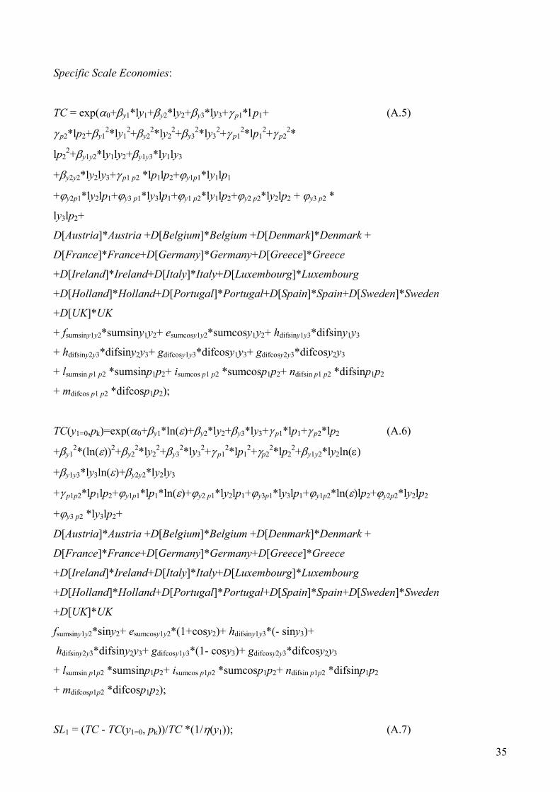
Specific Scale Economies:
TC = exp(α0+βy1*ly1+βy2*ly2+βy3*ly3+γ p1*l p1+ (A.5)
γ p2*lp2+βy12*ly1
2+βy22*ly2
2+βy32*ly3
2+γ p12*lp1
2+γ p22*
lp22+βy1y2*ly1ly2+βy1y3*ly1ly3
+βy2y2*ly2ly3+γ p1 p2 *lp1lp2+ϕy1p1*ly1lp1
+ϕy2p1*ly2lp1+ϕy3 p1*ly3lp1+ϕy1 p2*ly1lp2+ϕy2 p2*ly2lp2 + ϕy3 p2 *
ly3lp2+
D[Austria]*Austria +D[Belgium]*Belgium +D[Denmark]*Denmark +
D[France]*France+D[Germany]*Germany+D[Greece]*Greece
+D[Ireland]*Ireland+D[Italy]*Italy+D[Luxembourg]*Luxembourg
+D[Holland]*Holland+D[Portugal]*Portugal+D[Spain]*Spain+D[Sweden]*Sweden
+D[UK]*UK
+ fsumsiny1y2*sumsiny1y2+ esumcosy1y2*sumcosy1y2+ hdifsiny1y3*difsiny1y3
+ hdifsiny2y3*difsiny2y3+ gdifcosy1y3*difcosy1y3+ gdifcosy2y3*difcosy2y3
+ lsumsin p1 p2 *sumsinp1p2+ isumcos p1 p2 *sumcosp1p2+ ndifsin p1 p2 *difsinp1p2
+ mdifcos p1 p2 *difcosp1p2);
TC(y1=0,pk)=exp(α0+βy1*ln(ε)+βy2*ly2+βy3*ly3+γ p1*lp1+γ p2*lp2 (A.6)
+βy12*(ln(ε))2+βy2
2*ly22+βy3
2*ly32+γ p1
2*lp12+γp2
2*lp22+βy1y2*ly2ln(ε)
+βy1y3*ly3ln(ε)+βy2y2*ly2ly3
+γ p1p2*lp1lp2+ϕy1p1*lp1*ln(ε)+ϕy2 p1*ly2lp1+ϕy3p1*ly3lp1+ϕy1p2*ln(ε)lp2+ϕy2p2*ly2lp2
+ϕy3 p2 *ly3lp2+
D[Austria]*Austria +D[Belgium]*Belgium +D[Denmark]*Denmark +
D[France]*France+D[Germany]*Germany+D[Greece]*Greece
+D[Ireland]*Ireland+D[Italy]*Italy+D[Luxembourg]*Luxembourg
+D[Holland]*Holland+D[Portugal]*Portugal+D[Spain]*Spain+D[Sweden]*Sweden
+D[UK]*UK
fsumsiny1y2*siny2+ esumcosy1y2*(1+cosy2)+ hdifsiny1y3*(- siny3)+
hdifsiny2y3*difsiny2y3+ gdifcosy1y3*(1- cosy3)+ gdifcosy2y3*difcosy2y3
+ lsumsin p1p2 *sumsinp1p2+ isumcos p1p2 *sumcosp1p2+ ndifsin p1p2 *difsinp1p2
+ mdifcosp1p2 *difcosp1p2);
SL1 = (TC - TC(y1=0, pk))/TC *(1/η(y1)); (A.7)
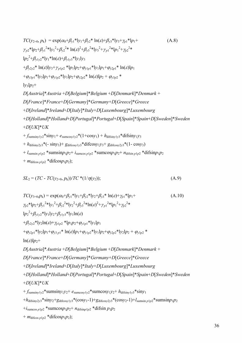
36
TC(y2=0, pk) = exp(α0+βy1*ly1+βy2* ln(ε)+βy3*ly3+γp1*lp1+ (A.8)
γ p2*lp2+βy12*ly1
2+βy22* ln(ε)2+βy3
2*ly32+γ p1
2*lp12+γp2
2*
lp22+βy1y2*ly1*ln(ε)+βy1y3*ly1ly3
+βy2y2* ln(ε)ly3+γ p1p2 *lp1lp2+ϕy1p1*ly1lp1+ϕy2p1* ln(ε)lp1
+ϕy3p1*ly3lp1+ϕy1p2*ly1lp2+ϕy2p2* ln(ε)lp2 + ϕy3p2 *
ly3lp2+
D[Austria]*Austria +D[Belgium]*Belgium +D[Denmark]*Denmark +
D[France]*France+D[Germany]*Germany+D[Greece]*Greece
+D[Ireland]*Ireland+D[Italy]*Italy+D[Luxembourg]*Luxembourg
+D[Holland]*Holland+D[Portugal]*Portugal+D[Spain]*Spain+D[Sweden]*Sweden
+D[UK]*UK
+ fsumsiny1y2*siny1+ esumcosy1y2*(1+cosy1) + hdifsiny1y3*difsiny1y3
+ hdifsiny2y3*(- siny3)+ gdifcosy1y3*difcosy1y3+ gdifcosy2y3*(1- cosy3)
+ lsumsin p1p2 *sumsinp1p2+ isumcos p1p2 *sumcosp1p2+ ndifsin p1p2 *difsinp1p2
+ mdifcos p1p2 *difcosp1p2);
SL2 = (TC - TC(y2=0, pk))/TC *(1/η(y2)); (A.9)
TC(y3=0,pk) = exp(α0+βy1*ly1+βy2*ly2+βy3* ln(ε)+γp1*lp1+ (A.10)
γp2*lp2+βy12*ly1
2+βy22*ly2
2+βy32*ln(ε)2+γ p1
2*lp12+γp2
2*
lp22+βy1y2*ly1ly2+βy1y3*ly1ln(ε)
+βy2y2*ly2ln(ε)+γp1p2 *lp1p2+ϕy1p1*ly1lp1
+ϕy2p1*ly2lp1+ϕy3 p1* ln(ε)lp1+ϕy1p2*ly1lp2+ϕy2p2*ly2lp2 + ϕy3p2 *
ln(ε)lp2+
D[Austria]*Austria +D[Belgium]*Belgium +D[Denmark]*Denmark +
D[France]*France+D[Germany]*Germany+D[Greece]*Greece
+D[Ireland]*Ireland+D[Italy]*Italy+D[Luxembourg]*Luxembourg
+D[Holland]*Holland+D[Portugal]*Portugal+D[Spain]*Spain+D[Sweden]*Sweden
+D[UK]*UK
+ fsumsiny1y2*sumsiny1y2+ esumcosy1y2*sumcosy1y2+ hdifsiny1y3*siny1
+hdifsiny2y3*siny2+gdifcosy1y3*(cosy1-1)+gdifcosy2y3*(cosy2-1)+lsumsin p1p2*sumsinp1p2
+isumcos p1p2 *sumcosp1p2+ ndifsinp1p2 *difsin p1p2
+ mdifcos p1p2 *difcosp1p2);
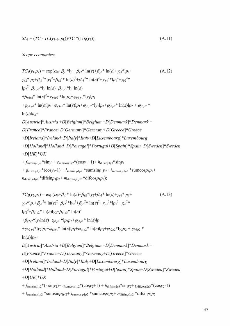
37
SL3 = (TC - TC(y3=0, pk))/TC *(1/η(y3)); (A.11)
Scope economies:
TC1(y1,pk) = exp(α0+βy1*ly1+βy2* ln(ε)+βy3* ln(ε)+γp1*lp1+ (A.12)
γp2*lp2+βy12*ly1
2+βy22* ln(ε)2+βy3
2* ln(ε)2+γ p12*lp1
2+γp22*
lp22+βy1y2*ly1ln(ε)+βy1y3*ly1ln(ε)
+βy2y2* ln(ε)2+γ p1p2 *lp1p2+ϕy1 p1*ly1lp1
+ϕy2 p1* ln(ε)lp1+ϕy3p1* ln(ε)lp1+ϕy1p2*ly1lp2+ϕy2p2* ln(ε)lp2 + ϕy3p2 *
ln(ε)lp2+
D[Austria]*Austria +D[Belgium]*Belgium +D[Denmark]*Denmark +
D[France]*France+D[Germany]*Germany+D[Greece]*Greece
+D[Ireland]*Ireland+D[Italy]*Italy+D[Luxembourg]*Luxembourg
+D[Holland]*Holland+D[Portugal]*Portugal+D[Spain]*Spain+D[Sweden]*Sweden
+D[UK]*UK
+ fsumsiny1y2*siny1+ esumcosy1y2*(cosy1+1)+ hdifsiny1y3*siny1
+ gdifcosy1y3*(cosy1-1) + lsumsin p1p2 *sumsinp1p2+ isumcos p1p2 *sumcosp1p2+
ndifsin p1p2 *difsinp1p2+ mdifcos p1p2 *difcosp1p2);
TC2(y2,pk) = exp(α0+βy1* ln(ε)+βy2*ly2+βy3* ln(ε)+γp1*lp1+ (A.13)
γp2*lp2+βy12* ln(ε)2+βy2
2*ly22+βy3
2* ln(ε)2+γ p12*lp1
2+γp22*
lp22+βy1y2* ln(ε)ly2+βy1y3* ln(ε)2
+βy2y2*ly2ln(ε)+γp1p2 *lp1p2+ϕy1p1* ln(ε)lp1
+ϕy2 p1*ly2lp1+ϕy3p1* ln(ε)lp1+ϕy1p2* ln(ε)lp2+ϕy2p2*ly2p2 + ϕy3p2 *
ln(ε)lp2+
D[Austria]*Austria +D[Belgium]*Belgium +D[Denmark]*Denmark +
D[France]*France+D[Germany]*Germany+D[Greece]*Greece
+D[Ireland]*Ireland+D[Italy]*Italy+D[Luxembourg]*Luxembourg
+D[Holland]*Holland+D[Portugal]*Portugal+D[Spain]*Spain+D[Sweden]*Sweden
+D[UK]*UK
+ fsumsiny1y2*(- siny2)+ esumcosy1y2*(cosy2+1) + hdifsiny2y3*siny2+ gdifcosy2y3*(cosy2-1)
+ lsumsin p1p2 *sumsinp1p2+ isumcos p1p2 *sumcosp1p2+ ndifsin p1p2 *difsinp1p2
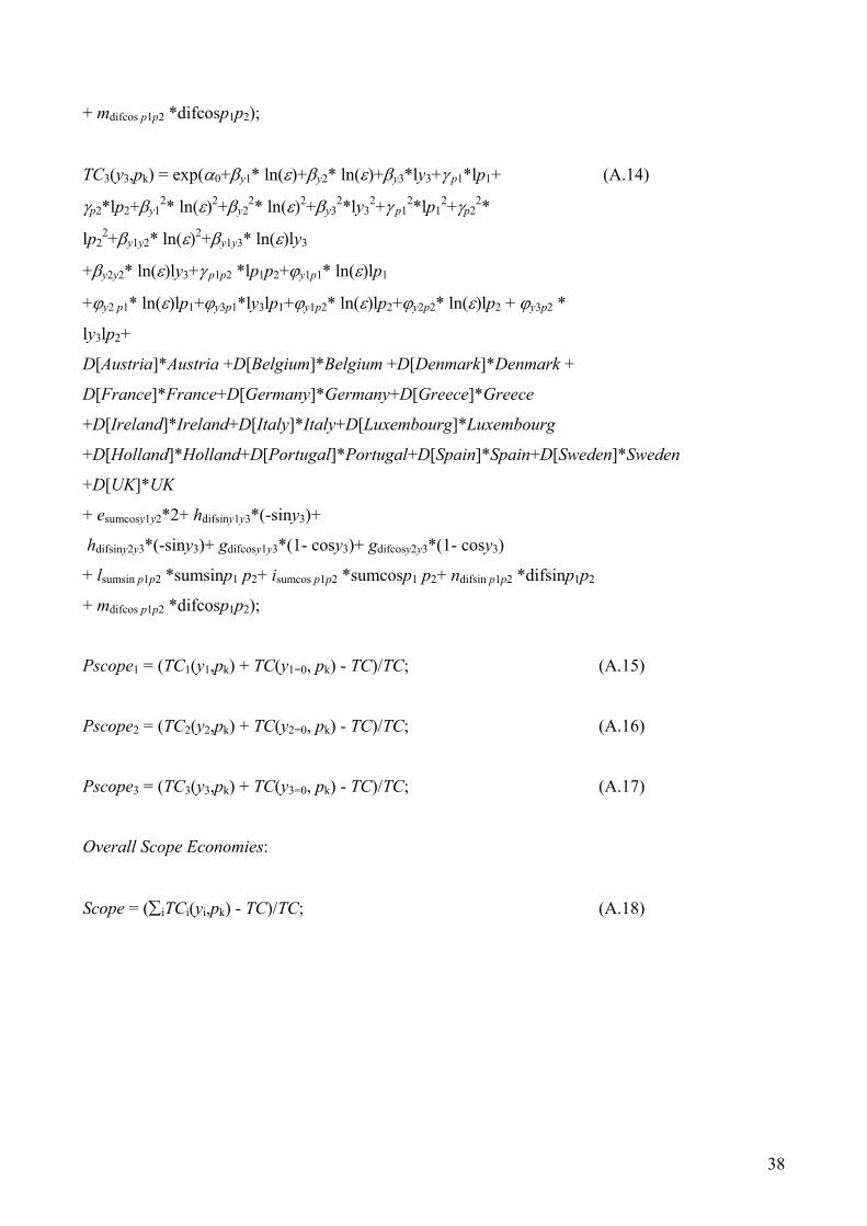
38
+ mdifcos p1p2 *difcosp1p2);
TC3(y3,pk) = exp(α0+βy1* ln(ε)+βy2* ln(ε)+βy3*ly3+γ p1*lp1+ (A.14)
γp2*lp2+βy12* ln(ε)2+βy2
2* ln(ε)2+βy32*ly3
2+γ p12*lp1
2+γp22*
lp22+βy1y2* ln(ε)2+βy1y3* ln(ε)ly3
+βy2y2* ln(ε)ly3+γ p1p2 *lp1p2+ϕy1p1* ln(ε)lp1
+ϕy2 p1* ln(ε)lp1+ϕy3p1*ly3lp1+ϕy1p2* ln(ε)lp2+ϕy2p2* ln(ε)lp2 + ϕy3p2 *
ly3lp2+
D[Austria]*Austria +D[Belgium]*Belgium +D[Denmark]*Denmark +
D[France]*France+D[Germany]*Germany+D[Greece]*Greece
+D[Ireland]*Ireland+D[Italy]*Italy+D[Luxembourg]*Luxembourg
+D[Holland]*Holland+D[Portugal]*Portugal+D[Spain]*Spain+D[Sweden]*Sweden
+D[UK]*UK
+ esumcosy1y2*2+ hdifsiny1y3*(-siny3)+
hdifsiny2y3*(-siny3)+ gdifcosy1y3*(1- cosy3)+ gdifcosy2y3*(1- cosy3)
+ lsumsin p1p2 *sumsinp1 p2+ isumcos p1p2 *sumcosp1 p2+ ndifsin p1p2 *difsinp1p2
+ mdifcos p1p2 *difcosp1p2);
Pscope1 = (TC1(y1,pk) + TC(y1=0, pk) - TC)/TC; (A.15)
Pscope2 = (TC2(y2,pk) + TC(y2=0, pk) - TC)/TC; (A.16)
Pscope3 = (TC3(y3,pk) + TC(y3=0, pk) - TC)/TC; (A.17)
Overall Scope Economies:
Scope = (∑iTCi(yi,pk) - TC)/TC; (A.18)
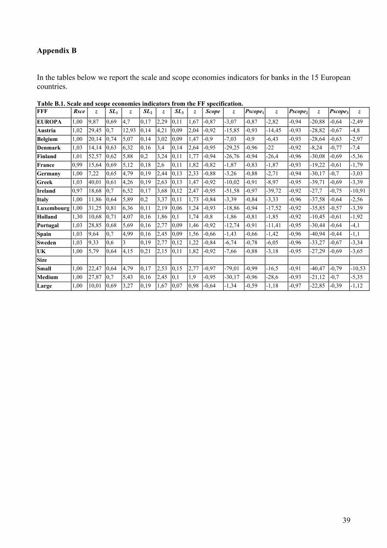
39
Appendix B In the tables below we report the scale and scope economies indicators for banks in the 15 European countries. Table B.1. Scale and scope economies indicators from the FF specification. FFF Rsce z SL1 z SL2 z SL3 z Scope z Pscope1 z Pscope2 z Pscope3 z
EUROPA 1,00 9,87 0,69 4,7 0,17 2,29 0,11 1,67 -0,87 -3,07 -0,87 -2,82 -0,94 -20,88 -0,64 -2,49 Austria 1,02 29,45 0,7 12,93 0,14 4,21 0,09 2,04 -0,92 -15,85 -0,93 -14,45 -0,93 -28,82 -0,67 -4,8 Belgium 1,00 20,14 0,74 5,07 0,14 3,02 0,09 1,47 -0,9 -7,03 -0,9 -6,43 -0,93 -28,64 -0,63 -2,97 Denmark 1,03 14,14 0,63 6,32 0,16 3,4 0,14 2,64 -0,95 -29,25 -0,96 -22 -0,92 -8,24 -0,77 -7,4 Finland 1,01 52,57 0,62 5,88 0,2 3,24 0,11 1,77 -0,94 -26,76 -0,94 -26,4 -0,96 -30,08 -0,69 -5,36 France 0,99 15,64 0,69 5,12 0,18 2,6 0,11 1,82 -0,82 -1,87 -0,83 -1,87 -0,93 -19,22 -0,61 -1,79 Germany 1,00 7,22 0,65 4,79 0,19 2,44 0,13 2,33 -0,88 -3,26 -0,88 -2,71 -0,94 -30,17 -0,7 -3,03 Greek 1,03 40,01 0,61 4,26 0,19 2,63 0,13 1,47 -0,92 -10,02 -0,91 -8,97 -0,95 -39,71 -0,69 -3,39 Ireland 0,97 18,68 0,7 6,52 0,17 3,68 0,12 2,47 -0,95 -51,58 -0,97 -39,72 -0,92 -27,7 -0,75 -10,91 Italy 1,00 11,86 0,64 5,89 0,2 3,37 0,11 1,73 -0,84 -3,39 -0,84 -3,33 -0,96 -37,58 -0,64 -2,56 Luxembourg 1,00 31,25 0,81 6,36 0,11 2,19 0,06 1,24 -0,93 -18,86 -0,94 -17,52 -0,92 -35,85 -0,57 -3,39 Holland 1,30 10,68 0,71 4,07 0,16 1,86 0,1 1,74 -0,8 -1,86 -0,81 -1,85 -0,92 -10,45 -0,61 -1,92 Portugal 1,03 28,85 0,68 5,69 0,16 2,77 0,09 1,46 -0,92 -12,74 -0,91 -11,41 -0,95 -30,44 -0,64 -4,1 Spain 1,03 9,64 0,7 4,99 0,16 2,45 0,09 1,56 -0,66 -1,43 -0,66 -1,42 -0,96 -40,94 -0,44 -1,1 Sweden 1,03 9,33 0,6 3 0,19 2,77 0,12 1,22 -0,84 -6,74 -0,78 -6,05 -0,96 -33,27 -0,67 -3,34 UK 1,00 5,79 0,64 4,15 0,21 2,15 0,11 1,82 -0,92 -7,66 -0,88 -3,18 -0,95 -27,29 -0,69 -3,65 Size Small 1,00 22,47 0,64 4,79 0,17 2,53 0,15 2,77 -0,97 -79,01 -0,99 -16,5 -0,91 -40,47 -0,79 -10,53 Medium 1,00 27,87 0,7 5,43 0,16 2,45 0,1 1,9 -0,95 -30,17 -0,96 -28,6 -0,93 -21,12 -0,7 -5,35 Large 1,00 10,01 0,69 3,27 0,19 1,67 0,07 0,98 -0,64 -1,34 -0,59 -1,18 -0,97 -22,85 -0,39 -1,12
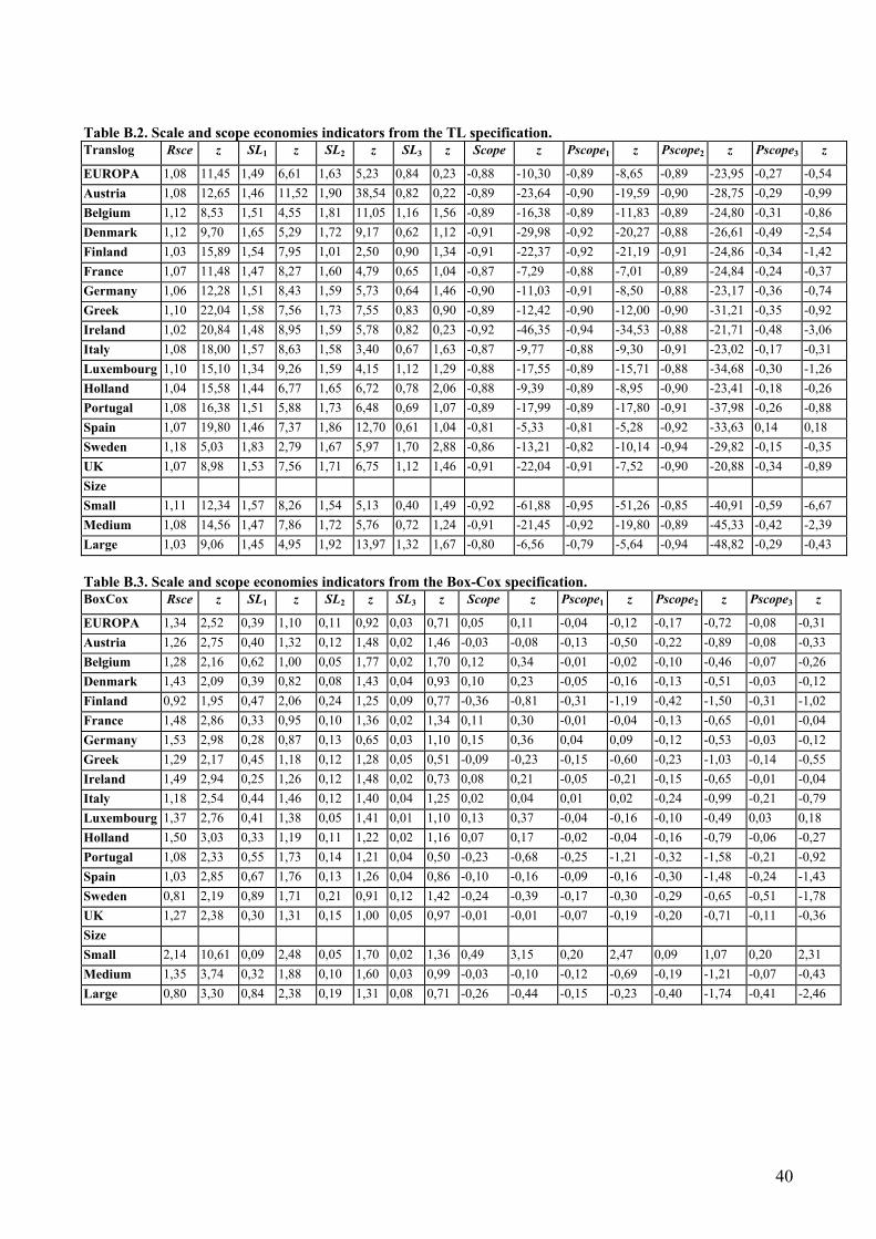
40
Table B.2. Scale and scope economies indicators from the TL specification. Translog Rsce z SL1 z SL2 z SL3 z Scope z Pscope1 z Pscope2 z Pscope3 z
EUROPA 1,08 11,45 1,49 6,61 1,63 5,23 0,84 0,23 -0,88 -10,30 -0,89 -8,65 -0,89 -23,95 -0,27 -0,54 Austria 1,08 12,65 1,46 11,52 1,90 38,54 0,82 0,22 -0,89 -23,64 -0,90 -19,59 -0,90 -28,75 -0,29 -0,99 Belgium 1,12 8,53 1,51 4,55 1,81 11,05 1,16 1,56 -0,89 -16,38 -0,89 -11,83 -0,89 -24,80 -0,31 -0,86 Denmark 1,12 9,70 1,65 5,29 1,72 9,17 0,62 1,12 -0,91 -29,98 -0,92 -20,27 -0,88 -26,61 -0,49 -2,54 Finland 1,03 15,89 1,54 7,95 1,01 2,50 0,90 1,34 -0,91 -22,37 -0,92 -21,19 -0,91 -24,86 -0,34 -1,42 France 1,07 11,48 1,47 8,27 1,60 4,79 0,65 1,04 -0,87 -7,29 -0,88 -7,01 -0,89 -24,84 -0,24 -0,37 Germany 1,06 12,28 1,51 8,43 1,59 5,73 0,64 1,46 -0,90 -11,03 -0,91 -8,50 -0,88 -23,17 -0,36 -0,74 Greek 1,10 22,04 1,58 7,56 1,73 7,55 0,83 0,90 -0,89 -12,42 -0,90 -12,00 -0,90 -31,21 -0,35 -0,92 Ireland 1,02 20,84 1,48 8,95 1,59 5,78 0,82 0,23 -0,92 -46,35 -0,94 -34,53 -0,88 -21,71 -0,48 -3,06 Italy 1,08 18,00 1,57 8,63 1,58 3,40 0,67 1,63 -0,87 -9,77 -0,88 -9,30 -0,91 -23,02 -0,17 -0,31 Luxembourg 1,10 15,10 1,34 9,26 1,59 4,15 1,12 1,29 -0,88 -17,55 -0,89 -15,71 -0,88 -34,68 -0,30 -1,26 Holland 1,04 15,58 1,44 6,77 1,65 6,72 0,78 2,06 -0,88 -9,39 -0,89 -8,95 -0,90 -23,41 -0,18 -0,26 Portugal 1,08 16,38 1,51 5,88 1,73 6,48 0,69 1,07 -0,89 -17,99 -0,89 -17,80 -0,91 -37,98 -0,26 -0,88 Spain 1,07 19,80 1,46 7,37 1,86 12,70 0,61 1,04 -0,81 -5,33 -0,81 -5,28 -0,92 -33,63 0,14 0,18 Sweden 1,18 5,03 1,83 2,79 1,67 5,97 1,70 2,88 -0,86 -13,21 -0,82 -10,14 -0,94 -29,82 -0,15 -0,35 UK 1,07 8,98 1,53 7,56 1,71 6,75 1,12 1,46 -0,91 -22,04 -0,91 -7,52 -0,90 -20,88 -0,34 -0,89 Size Small 1,11 12,34 1,57 8,26 1,54 5,13 0,40 1,49 -0,92 -61,88 -0,95 -51,26 -0,85 -40,91 -0,59 -6,67 Medium 1,08 14,56 1,47 7,86 1,72 5,76 0,72 1,24 -0,91 -21,45 -0,92 -19,80 -0,89 -45,33 -0,42 -2,39 Large 1,03 9,06 1,45 4,95 1,92 13,97 1,32 1,67 -0,80 -6,56 -0,79 -5,64 -0,94 -48,82 -0,29 -0,43 Table B.3. Scale and scope economies indicators from the Box-Cox specification. BoxCox Rsce z SL1 z SL2 z SL3 z Scope z Pscope1 z Pscope2 z Pscope3 z
EUROPA 1,34 2,52 0,39 1,10 0,11 0,92 0,03 0,71 0,05 0,11 -0,04 -0,12 -0,17 -0,72 -0,08 -0,31 Austria 1,26 2,75 0,40 1,32 0,12 1,48 0,02 1,46 -0,03 -0,08 -0,13 -0,50 -0,22 -0,89 -0,08 -0,33 Belgium 1,28 2,16 0,62 1,00 0,05 1,77 0,02 1,70 0,12 0,34 -0,01 -0,02 -0,10 -0,46 -0,07 -0,26 Denmark 1,43 2,09 0,39 0,82 0,08 1,43 0,04 0,93 0,10 0,23 -0,05 -0,16 -0,13 -0,51 -0,03 -0,12 Finland 0,92 1,95 0,47 2,06 0,24 1,25 0,09 0,77 -0,36 -0,81 -0,31 -1,19 -0,42 -1,50 -0,31 -1,02 France 1,48 2,86 0,33 0,95 0,10 1,36 0,02 1,34 0,11 0,30 -0,01 -0,04 -0,13 -0,65 -0,01 -0,04 Germany 1,53 2,98 0,28 0,87 0,13 0,65 0,03 1,10 0,15 0,36 0,04 0,09 -0,12 -0,53 -0,03 -0,12 Greek 1,29 2,17 0,45 1,18 0,12 1,28 0,05 0,51 -0,09 -0,23 -0,15 -0,60 -0,23 -1,03 -0,14 -0,55 Ireland 1,49 2,94 0,25 1,26 0,12 1,48 0,02 0,73 0,08 0,21 -0,05 -0,21 -0,15 -0,65 -0,01 -0,04 Italy 1,18 2,54 0,44 1,46 0,12 1,40 0,04 1,25 0,02 0,04 0,01 0,02 -0,24 -0,99 -0,21 -0,79 Luxembourg 1,37 2,76 0,41 1,38 0,05 1,41 0,01 1,10 0,13 0,37 -0,04 -0,16 -0,10 -0,49 0,03 0,18 Holland 1,50 3,03 0,33 1,19 0,11 1,22 0,02 1,16 0,07 0,17 -0,02 -0,04 -0,16 -0,79 -0,06 -0,27 Portugal 1,08 2,33 0,55 1,73 0,14 1,21 0,04 0,50 -0,23 -0,68 -0,25 -1,21 -0,32 -1,58 -0,21 -0,92 Spain 1,03 2,85 0,67 1,76 0,13 1,26 0,04 0,86 -0,10 -0,16 -0,09 -0,16 -0,30 -1,48 -0,24 -1,43 Sweden 0,81 2,19 0,89 1,71 0,21 0,91 0,12 1,42 -0,24 -0,39 -0,17 -0,30 -0,29 -0,65 -0,51 -1,78 UK 1,27 2,38 0,30 1,31 0,15 1,00 0,05 0,97 -0,01 -0,01 -0,07 -0,19 -0,20 -0,71 -0,11 -0,36 Size Small 2,14 10,61 0,09 2,48 0,05 1,70 0,02 1,36 0,49 3,15 0,20 2,47 0,09 1,07 0,20 2,31 Medium 1,35 3,74 0,32 1,88 0,10 1,60 0,03 0,99 -0,03 -0,10 -0,12 -0,69 -0,19 -1,21 -0,07 -0,43 Large 0,80 3,30 0,84 2,38 0,19 1,31 0,08 0,71 -0,26 -0,44 -0,15 -0,23 -0,40 -1,74 -0,41 -2,46
![Untitled-1 [] · CHOCOMILO; Bouillon - MAGGI CUBE, MAGGI CHICKEN, MAGGI CRAYFISH, MAGGI MIX'PY; and table water ... and marketing company](https://img.pdfslide.net/doc/110x75/5aedc9577f8b9a6625906f43/untitled-1-bouillon-maggi-cube-maggi-chicken-maggi-crayfish-maggi-mixpy.jpg)