Excited state, non-adiabatic dynamics of large photoswitchable molecules using achemically transferable machine learning potential

Simon Axelrod,1, 2 Eugene Shakhnovich,1 and Rafael Gómez-Bombarelli2, ∗

1Department of Chemistry and Chemical Biology, Harvard University, Cambridge, MA, 021382Department of Materials Science and Engineering,

Massachusetts Institute of Technology, Cambridge, MA, 02139(Dated: August 12, 2021)

Light-induced chemical processes are ubiquitous in nature and have widespread technologicalapplications. For example, the photoisomerization of azobenzene allows a drug with an azo scaffoldto be activated with light. In principle, photoswitches with useful reactive properties, such ashigh isomerization yields, can be identified through virtual screening with reactive simulations. Inpractice these simulations are rarely used for screening, since they require hundreds of trajectoriesand expensive quantum chemical methods to account for non-adiabatic excited state effects. Here weintroduce a neural network potential to accelerate such simulations for azobenzene derivatives. Themodel, which is based on diabatic states, is called the diabatic artificial neural network (DANN).The network is six orders of magnitude faster than the quantum chemistry method used for training.DANN is transferable to molecules outside the training set, predicting quantum yields for unseenspecies that are correlated with experiment. We use the model to virtually screen 3,100 hypotheticalmolecules, and identify several species with extremely high quantum yields. Our results pave theway for fast and accurate virtual screening of photoactive compounds.

Light is a powerful tool for manipulating molecular sys-tems. It can be controlled with high spatial, spectraland temporal precision to facilitate a variety of processes,including energy transfer, intermolecular reactions, andphotoisomerization [1]. Such processes are used in areasas diverse as synthesis, energy storage, display technol-ogy, biological imaging, diagnostics and medicine [1–3].Photoactive drugs, for instance, are photoswitchable com-pounds whose bioactivity can be toggled through light-induced isomerization. Precise spatiotemporal control ofbioactivity allows photoactive drugs to be delivered inhigh doses with minimal off-target activity and side ef-fects. Such therapeutics are a promising path for thetreatment of cancer, neurodegenerative diseases, bacte-rial infections, diabetes, and blindness [4].

Theory plays a key role in explaining and predictingphotochemistry because empirical heuristics learned fromthermally activated ground state processes typically donot apply to excited states [3]. Computer simulationsbased on quantum mechanics can achieve impressive accu-racy in the prediction of experimental observables. Theseinclude the isomerization efficiency and absorption spec-trum of photoswitchable compounds [5, 6], which are keyquantities in the design of photoactive drugs.

However, ab initio methods in photochemistry areseverely limited by their computational cost [7]. In order

∗ Corresponding author: rafagb@mit.edu

to gather meaningful statistics for one molecule, hundredsof replicate simulations are needed, each of which involvesthousands of electronic structure calculations performedin series with sub-femtosecond timesteps. The individ-ual quantum chemical calculations are particularly de-manding, requiring excited state gradients, interstate cou-plings, and some treatment of multireference effects. Us-ing ab initio methods to compute photochemical proper-ties of tens or hundreds molecules is impractical, and pho-todynamic simulations have not yet been used for large-scale virtual screening.

Many methods have been developed to alleviate thissteep computational cost. Semi-empirical methods [8–10] provide qualitatively correct results across many sys-tems, but are ultimately bounded by their approxima-tions, with average energy errors of 15 kcal/mol [9]. Otherapproaches focus on hardware and software development[11, 12], but cannot match the speed of semi-empiricalmethods.

A different approach is to use data-driven, non-parametric models in place of quantum chemistry (QC)calculations. Machine learning (ML) models trained onquantum chemical data can now routinely predict groundstate energies and forces with sub-chemical accuracy [13–15], and take only milliseconds to make predictions.These models have been successfully used in a variety ofground state simulations [14, 16–18]. They have also beenused to accelerate non-adiabatic simulations in a numberof model systems [19–24]. However, excited state ML hasnot yet offered affordable photodynamics for hundreds of

arX

iv:2

108.

0487

9v1

[ph

ysic

s.ch

em-p

h] 1

0 A

ug 2

021

2

molecules of realistic size, which is the ultimate goal forpredictive simulation in photopharmacology. Further, noexcited-state interatomic potentials have been developedthat are transferable to different compounds. They there-fore require thousands of QC calculations for every newspecies to serve as training data.

Here we make significant progress toward affordable,large-scale photochemical simulations and virtual screen-ing with ML. To develop a transferable potential we fo-cus on molecules from the same chemical family, study-ing derivatives of azobenzene, a prototypical photoswitch.The derivatives studied here contain up to 100 atoms,making them the largest systems fit with excited-stateML potentials to date. Combining an equivariant neuralnetwork [14] and a physics-informed diabatic model, to-gether with data generated by combinatorial sampling ofchemical space and configurational sampling through ac-tive learning, we produce a model that is transferable tolarge, unseen derivatives of azobenzene. This yields com-putational savings in excess of six orders of magnitude.Predicted isomerization quantum yields of unseen speciesare well-correlated with experimental values. The modelis used to predict the quantum yield for over 3,100 hypo-thetical species, revealing rare molecules with extremelyhigh cis-to-trans and trans-to-cis quantum yields.

RESULTS

A. Azobenzene photoswitches

This work focuses on the photoswitching of azobenzenederivatives, but the methods are general and can be ap-plied to other chemistries and other excited state pro-cesses. Azobenzene derivatives can exist as cis and transconformers. The conformations are local minima in theground state, but not in the excited state. Photoexcita-tion of either can therefore induce isomerization into theother (see the potential energy schematics in Figs. 1(a)and 2(b)). A key experimental observable is the quantumyield, defined as the probability that excitation leads toisomerization. The yield depends critically on the dy-namics near conical intersections (CIs), configurations inwhich the excitation energy is zero. In these regions theelectrons can return to the ground state with non-zeroprobability. This non-adiabatic transition can be modeledwith surface hopping [25], in which independent trajecto-ries are simulated with stochastic hops between potentialenergy surfaces (PESs). Depending on the curvature ofthe PESs and the location of the hop, a trajectory canend with the original isomer or with a new isomer (Figs.1(a) and 2(b)). The quantum yield is the proportion of

Figure 1. Depiction of the potential energy surfaces in azoben-zene derivatives. (a) S0 and S1 adiabatic energies, with theCI region shaded in gray. Initial excitation is shown with avertical zigzag line. Trajectories prior to hopping are shownin black. Reactive and unreactive trajectories after hoppingare shown in green and yellow, respectively. (b) Diabatic en-ergies dnm ≡ (Hd)nm. The diagonal diabatic elements crossand become re-ordered along the isomerization coordinate. ACI occurs when the diagonal diabatic elements cross and theoff-diagonal element becomes zero.

trajectories that end in a new isomer. Our goal is topredict the quantum yield of azobenzene derivatives afterexcitation from the singlet ground state (S0) to the firstsinglet excited state (S1). This can be accomplished withthe surface hopping approach described above, using anML model to generate the PESs.

B. ML architecture and training

Our model is based on the PaiNN neural network [14],which uses equivariant message-passing to predict molec-ular properties. In this approach one first generates afeature vector for each atom using its atomic number.The vector is then updated through a set of neural net-work operations involving “messages”, which incorporatethe distance, orientation, and features of atoms within acutoff distance. A series of updates leads to informationbeing aggregated from increasingly distant atoms. Oncethe updates are complete, the atomic features are mappedto molecular energies using a neural network.

This architecture can be used to predict energies and,through automatic differentiation, the forces for eachstate. However, models that predict adiabatic energieshave a basic shortcoming for non-adiabatic molecular dy-namics (NAMD). Since surface hopping is controlled bythe energy gap when it is close to zero, small errors in theenergies can lead to exponentially large errors in the hop-

3

!!

×3

$! %!"

+

readout

update

message

update

message

diagonalize

+ +

+

+

+ +

… readout

&#$&%%Σ!Σ!

'&

a b

Figure 2. (a) Schematic of the DANN architecture, which is based on the PaiNN model. Scalar atomic features si and vectorialatomic features ~vi are updated through messages from neighboring atoms. The si are then mapped to atomic energies, whichare summed to produce the diabatic Hamiltonian Hd. The diabatic matrix is diagonalized to produce adiabatic quantities. (b)Schematic of the active learning loop. Geometries and QC data are first generated through ab initio NAMD, normal modesampling, and inversion/rotation about the central N=N double bond. Two neural networks are then trained on the data andused to perform NN-NAMD. Newly generated geometries with high committee variance and/or low predicted gaps receive QCcalculations. The new calculations are added to the training data, the networks are retrained, and the cycle is repeated untilconvergence.

ping probability [26]. This in turn can cause large errorsin observable quantities like the quantum yield. Further,since CIs are non-differentiable cusps in the energy gap,they are difficult to fit with neural networks. For N atomsin a molecule, the network must predict two different en-ergies that are exactly equal in 3N − 8 dimensions. Wehave found this to be particularly challenging for transspecies that are outside the training set. As shown inSupplementary Sec. 3, small errors in the gap lead to theincorrect prediction that many species never hop to theground state.

To remedy this issue we introduce a model based ondiabatic states, which we call DANN (diabatic artificialneural network ; Fig. 2(a)). The approach builds on previ-ous work using neural networks for diabatization [27–29].The diabatic energies form a non-diagonal Hamiltonianmatrix, Hd, which is diagonalized to yield adiabatic ener-gies. When a 2×2 sub-block of Hd has diagonal elementsthat cross, and off-diagonal elements that pass through

zero, a CI cusp is generated (Fig. 1). The diabatic en-ergies that generate the cusp are smooth, which makesthem easier to fit with an interpolating function than theadiabatic energies. Smoothness is imposed through a lossfunction that minimizes the non-adiabatic coupling vector(NACV) in the diabatic basis. The NACV measures thechange in overlap between two wavefunctions after a smallnuclear displacement. If the NACV between two statesis zero, then their wavefunctions must change slowly inresponse to a nuclear perturbation. Therefore, their en-ergies cannot form the cusp in Fig. 1(a), and must insteadresemble the smooth energies in Fig. 1(b).

The DANN model was trained on spin-flip TDDFT(SF-TDDFT) [30] calculations for 641,359 geometries, us-ing the 6-31G* basis [31] and BHHLYP [32] functional.Unlike traditional TDDFT [33], SF-TDDFT provides anaccurate description of the CI region [34], and, unlikemulti-reference methods, is fairly fast and requires nomanual parameter selection. The configurations were

4

E0 E1 ∆E01 (∆E01)smalla ~F0

~F1 ~g01

Seen speciesMAE (↓) 0.86 1.01 0.75 0.47 1.00 1.17 0.87R2 (↑) 1.00 1.00 1.00 0.97 0.99 0.99 0.84

Unseen speciesMAE (↓) 3.06 3.77 1.89 0.97 1.72 2.31 1.36R2 (↑) 0.99 0.98 0.98 0.95 0.97 0.86 0.50

a For these R2 calculations, we computed the total sum of squares using mean{∆E01} instead of mean{(∆E01)small}. The meanpredictor should not know a priori which gaps are small, and hence should predict the mean of all gaps.

Table I. Mean absolute error (MAE) and coefficient of determination (R2) of the DANN model for various quantities. Unitsare kcal/mol for energies and kcal/mol/Å for forces and force couplings. Ei are energies, ~Fi are forces, ∆E01 is the energy gap,and ~g01 is the force NACV. (∆E01)small denotes the energy gap when it is under 4.6 kcal/mol (0.2 eV).

sampled from 8,269 azobenzene derivatives, of which 164were taken from the experimental literature. The remain-ing molecules were generated from combinatorial substi-tution using common literature patterns (SupplementaryTables S6 and S7).

C. Validation

To test whether the model could reproduce experimen-tal results for unseen molecules, we evaluated it on speciesthat were outside the training set. The test set contained40 species (20 cis/trans pairs), including 33 with exper-imental S1 quantum yields in non-polar solution. Non-polar solution was chosen because it is the closest to thegas-phase conditions simulated here. We note that solventeffects can be easily incorporated into the model throughtransfer learning to implicit solvent calculations. This haspreviously been done with only a small proportion of thetraining set [16].

The performance of the model is summarized in TableI. Statistics are shown for both seen and unseen species.The former contains species that are in the training set,but geometries that are outside of it. The geometries wereselected with the balanced sampling criteria described inSupplementary Sec. 6. Geometries from unseen specieswere generated with neural network NAMD (NN-NAMD)using the final trained model. Half of the NN-NAMD ge-ometries were selected randomly from the full trajectoryand half by proximity to a CI (Eq. (S19)). 100 configu-rations were chosen for each molecule.

For species in the training set, all quantities are ac-curate to within approximately 1 kcal/mol(/Å). Apartfrom the NACV, all quantities have R2 correlation coef-ficients close to 1. The R2 of the NACV is 0.84. Thismay be somewhat low because diabatization cannot re-move the curl component of the NACV in the diabatic

basis [35]. This would also explain the low R2 value forthe NACV in Ref. [22], which computed it as the gradi-ent of a scalar. For molecules outside the training set, allquantities apart from the energies have an error below 3kcal/mol(/Å). The energy gaps and ground state forceshave R2 correlation coefficients near 1. The gap error of1.89 kcal/mol should be contrasted with the error of 15kcal/mol in Ref. [9], which applied semi-empirical meth-ods to azobenzene. The errors in the excited state forcesare slightly larger, but still quite low. The correlation co-efficient for the NACV is rather poor. However, as shownin Supplementary Sec. 3, the yields predicted by themodel are similar between NAMD methods that use theNACV and those that use only energies and forces. Hencethe low NACV correlation does not negatively impact thepredicted quantum yields.

Figure 3(a) shows snapshots from an example NN-NAMD trajectory, and panel (b) shows an example ofthe hopping geometries. Reactive hopping geometries areshown on top, and non-reactive ones are shown below.The molecule is the (aminomethyl)pyridine derivative 26,with the species numbering given in Supplementary Ta-bles S8 and S9. The overlays show cis-trans isomerizationproceeding through inversion-assisted rotation, consistentwith previous work [36]. The dominant motion is rota-tion, with the CNNC dihedral angle increasing in mag-nitude from −10◦ at equilibrium to −86◦ at the hoppingpoints. Significant changes also occur in the CNN andNNC angles, with each transitioning from 123◦ to either113◦ or 135◦.

The predicted PES in the branching space (~g,~h) isshown beside the geometries. ~g is the direction of theforce coupling and ~h ∝ ∇R(∆E01) is the direction of thegap gradient. Each vector was computed with automaticdifferentiation using Eq. (1). The diabatic energies, adi-abatic energies, and gap are shown from top to bottom.We see that the model generates a true CI, in which the

5

Figure 3. (a) Selected trajectory frames for a molecule outside the training set. The top panels show the S0 and S1 energyas a function of time. A yellow dot indicates the time at which the snapshot below was taken. (b) Left: Overlay of hoppinggeometries from reactive (top) and unreactive (bottom) trajectories. Right: PES as a function of branching plane coordinates atone of the reactive hopping geometries. Diabatic energies, adiabatic energies, and adiabatic gaps are shown from top to bottom.The diabatic coupling is shown in gray. (c) Predicted vs. experimental quantum yield for 33 species outside the training set.The R2 value and Spearman rank correlation ρ are both shown. Color-coded data points are defined below. (d) Node time forQC and ML calculations.

S0 and S1 energies are exactly equal. Further, the degen-eracy is lifted in both the ~g- and ~h-directions, so that theS1 energy and gap each form a characteristic cone. Thesehallmarks of CIs are built into the model because the adi-abatic energies are eigenvalues of a diabatic matrix. Forexample, the cone emerges from the fact that d11−d00 andd01 each pass linearly through zero in different directions[37].

Figure 3(c) indicates that the predicted and experimen-tal quantum yields of unseen species are correlated. TheR2 value is 0.39, and the Spearman rank correlation coef-ficient ρ is 0.76. The R2 value is quite high when consid-ering that the experimental measurements used a varietyof solvents and methods. The Spearman coefficient mea-sures the accuracy with which the model ranks speciesby quantum yield. ρ only compares orderings, making itmore forgiving than R2 and a more relevant metric forvirtual screening. Since cis isomers have yields 2-3 timeshigher than trans isomers, the high value of ρ means thatthe model properly separates the isomers into low- andhigh-yield groups.

Further, as shown in Fig. S4, the model producesmeaningful rankings among trans species (ρ=0.40). It islargely able to differentiate between high- and low-yieldtrans derivatives. Several such molecules are of inter-est. They are color-coded in the plots, with the legend

given below. A full list of predictions is given in TableS8. We see, for example, that the (aminomethyl)pyridinederivatives 1 and 35 are both predicted to have near-zeroyields. These species do not isomerize from trans to cis,because strong N-H hydrogen bonds lock the planar transconformation in place [38]. Replacing the NH group in1 with N− CH3 gives species 25. This molecule isomer-izes because there is no hydrogen bonding. This, too,is predicted by the model. Further, the hepta-tert-butylderivative 17 has an experimental and predicted yield ofzero. This is likely because of steric interactions amongthe bulky tert-butyl groups. While able to account forthese two different mechanisms, the model fails to predictthe subtle electronic effects in species 11 and 29. Reso-nance interactions between oxygen lone pairs and the azogroup modify the PES, such that there is no rotationalCI [39]. There is instead a concerted inversion CI, whichoccurs too early along the path between trans and cis toallow for isomerization. The changes in the PES may ei-ther be too small or too specific to the substituents forthe model to predict without fine tuning. Finally, deriva-tives with high yields are partly distinguished from thosewith low but non-zero yields. An example is 21, whoseexperimental yield of 0.1 is half that of trans-azobenzene.The model properly identifies this molecule as having alow yield, but also mistakenly does the same for several

6

Figure 4. Results of virtual screening. Species of interest are circled in gray and shown below the plots. (a) Predicted yieldvs. excitation energy for cis derivatives. (b) Predicted yield vs. stability for cis derivatives. (c)-(d) As in (a)-(b), but for transderivatives.

high-yield species. The accuracy for unseen species couldalways be improved with transfer learning, in which themodel is fine-tuned with a small number of calculationsfrom a single molecule. This would increase the compu-tational cost, but would still be orders of magnitude lessexpensive than ab initio NAMD.

While meaningful correlations are produced for transspecies, the same is not true of cis molecules (ρ = 0.02).This may be because there are no cis derivatives with zeroyield. Nevertheless, the model properly identifies 20 ashaving the highest yield. Further, it does not mistakenlyassign a zero yield to any derivative. This is noteworthybecause, as shown in Fig. 4(a) and (b), several hypotheti-cal cis species are predicted to have zero yield. Synthesisof non-switching cis derivatives and comparison to pre-dictions could therefore be of interest in the future.

Figure 3(d) shows that NN-NAMD is extremely fast.The plot shows the node time, defined as tcalc/ncalc, wheretcalc is the calculation time per geometry, and ncalc is thenumber of parallel calculations that can be performed ona single node. We see that ML speeds up calculationsby a remarkable five to six orders of magnitude. The di-rect comparison of the pre-trained model node times andQC node times is appropriate because the model gener-alizes to unseen species. This means that it incurs noextra QC cost for any future simulations. The minimumspeedup corresponds to the smallest molecules (14 heavyatoms or 24 total atoms), and the maximum to the largestmolecules (70 heavy atoms or 99 total atoms). This re-flects the different scaling of the QC and ML calcula-tions. Empirically we see that DANN scales as N0.49 forN heavy atoms, while SF-TDDFT scales as N2.8.

D. Virtual screening

Having shown that the model is fast and generalizesin the chemical and configurational space of azobenzenes,we next used it for virtual screening of hypothetical com-pounds. We first retrained the network on all availabledata, including species that were originally held out. Wethen predicted the quantum yields of 3,100 combinato-rial species generated through literature-informed substi-tution patterns, as in Ref. [40]. This screen served twopurposes. The first was to gather statistics about thedistribution of photophysical properties of azobenzenesat a scale not accessible to experiments or traditionalsimulations. The second was to identify molecules withrare desirable properties. In particular, we sought to findmolecules with high c −→ t or t −→ c quantum yields andredshifted absorption spectra. The former is importantbecause increasing the ratio QYa−→b /QYb−→a, where QYis the quantum yield, can lead to more complete a−→btransformation under steady state illumination. This iscritical for precise spatial control of drug activity whenthe two isomers have different biological effects [41]. Red-shifting is a crucial requirement for photo-active drugs,since human tissue is transparent only in the near-IR [41].

The results are shown in Fig. 4. Panels (a) and (c)show the predicted yield vs. mean gap. For each specieswe averaged the gap over the configurations sampled dur-ing neural network ground state MD. The thermal aver-aging led to a typical blueshift of 0.2-0.3 eV relative to thegaps of single equilibrium geometries. The mean excita-tion energies are 2.95 eV for cis derivatives and 2.84 eV fortrans species. The average gaps and their differences are

7

Figure 5. Violin plots of the CNNC dihedral angle vs. time for several compounds of interest. Reactive and non-reactiveNN-NAMD trajectories are shown in red and blue, respectively. The violin width at a given dihedral angle indicates the densityof trajectories with that angle. The predicted yield of each compound is shown above the plots. (a) Cis azobenzene. (b)-(c)Two cis derivatives. (d) Trans azobenzene. (e)-(f) Two trans derivatives. For ease of visualization we have used the range[−180, 180] for cis dihedral angles and [0, 360] for trans dihedral angles.

quite similar to experimental measurements for azoben-zene [42]. The average c→ t and t→ c yields are 0.54 and0.24, respectively, again consistent with non-substitutedazobenzene [42]. The mean (median) proportion of tra-jectories ending in the ground state after 2 ps is 92%(100%) for cis species and 31% (17%) for trans species.The standard deviations are 25% and 30%, respectively.

Panels (b) and (d) show the yield plotted against theisomeric stability, defined as Etrans − Ecis for trans iso-mers and Ecis − Etrans for cis isomers. The energy Eis the median value of the configurations sampled in theground state; we used the median to reduce the effect ofoutlier geometries. On average the trans isomers are morestable than the cis isomers by 0.66 eV (15.3 kcal/mol),which is similar to experimental values over 10 kcal/molfor azobenzene [43]. The stability is of interest for threereasons. First, a large absolute value indicates that oneisomer is dominant at room temperature. This is essentialfor photoactive drugs, and is the case for regular azoben-zene. Second, an inverted stability, in which cis is morestable than trans, allows for stronger absorption at longerwavelengths. This is because the dipole-forbidden n− π∗(S1) transition is significantly stronger for cis than fortrans [42]. Third, in photopharmacology, one often wantsto deliver a drug in inactive form, and activate it withlight in a localized region. If trans happens to be activeand cis inactive, then localized activation is only possibleif cis is more stable.

Several species of interest are shown in Fig. 4. Themolecules 165 and 166 have predicted yields of 0.75 ±0.06 and 0.72 ± 0.06, respectively, which are well abovethe cis average of 0.55. The species 169 and 170 havepredicted yields of 0.66 ± 0.07 and 0.63 ± 0.10, respec-tively, which are three times the average trans yield.Molecule 167 is highly redshifted, with a mean predictedgap of 2.26 eV (548 nm), and a standard deviation of0.87 eV. QC calculations on the neural network geome-tries gave a gap of 2.26 ± 0.61 eV, in good agreementwith predictions. The mean gap is lower than the me-dian of 2.52 eV, which reflects the presence of severalultra-low gap structures. The low gap and large variancemean that 167 may be able to absorb in the near IR. Theredshifting is likely because of the six electron donatinggroups, which increase the HOMO energy, together withthe crowding of the four ortho substituents. The latterdistorts the molecule, leading to twisted configurationswith smaller gaps. Finally, species 168 is more stablein cis form than trans form. The predicted cis stabilityis −0.79 eV (−18 kcal/mol), in good agreement with theQC prediction of −0.92 eV (−21 kcal/mol). As mentionedabove, this inverted stability can be a desirable propertyfor photopharmacology.

Figure 5 shows the distribution of CNNC dihedral an-gles vs. time for the high-yield species, computed withNN-NAMD. Compared to cis azobenzene, the density ofangles in 165 is initially rather narrow (Fig. 5(b)). The

8

localization of trajectories near −90◦, without the small-magnitude angles of azobenzene, may explain the highyield. 166 appears to rotate further than cis azobenzeneat early times (Fig. 5(c)). Its high yield could thereforebe because of a higher velocity in the direction of rotation.

In trans azobenzene, many of the non-reactive trajec-tories remain localized at 180◦, while the reactive trajec-tories rotate by 90◦ (Fig. 5(d)). This is consistent withRef. [6], which identified a non-reactive planar CI and areactive twisted CI as the main hopping points for transazobenzene. The non-reactive CI leads exclusively backto trans, while the reactive CI leads to cis and trans indifferent proportions. By contrast, all non-reactive trajec-tories for 169 rotate significantly (Fig. 5(e)). This sug-gests that the non-reactive planar CI may be bypassed,thereby increasing the yield. This is consistent with thenon-planarity of the 169 equilibrium structure due to thebulky ortho groups. A similar process seems to be tak-ing place for 170, even though the equilibrium structureis planar (Fig. 5(f)). While the effect is smaller, thenon-reactive trajectories of 170 also involve more rota-tion than those of azobenzene.

E. Discussion and directions for improvement

The DANN model shows high accuracy and transfer-ability among azobenzene derivatives. However, it cannotbe applied to other chemical families without additionaltraining data. Further, as shown in Supplementary Sec.3, it substantially overestimates the excited state lifetimefor a number of trans derivatives. On the other hand,semi-empirical methods provide qualitatively correct pre-dictions across a variety of chemistries, but cannot matchDANN’s in-domain accuracy, and cannot be improvedwith more reference data. Adding features from semi-empirical calculations, as done in the OrbNet model [44],may therefore prove useful in the future. Recent develop-ments accounting for non-local effects and spin states haveimproved neural network transferability [15], and couldalso be beneficial for excited states. The model could befurther improved with high-accuracy multi-reference cal-culations, solvent effects, and the inclusion of the brightS2 state. Active learning could be accelerated throughdifferentiable sampling with adversarial uncertainty at-tacks [45], which would improve the excited state life-times. Transfer learning could also be used to improveperformance for specific molecules. Only a small number

of ab initio calculations would be required to fine-tunethe model for an individual species.

Diabatization may also prove to be useful for reactiveground states. Reaction barriers can often be understoodas transitions from one diabatic state to another [35]. Thediabatic basis may make reactive surfaces easier to fit withneural networks.

CONCLUSION

We have introduced a diabatic multi-state neuralnetwork potential trained on over 640,000 geometries atthe SF-TDDFT BHHLYP/6-31G* level of theory, cov-ering over 8,000 unique azobenzene molecules. We usedNN-NAMD to predict the isomerization quantum yieldsof derivatives outside the training set, and the resultswere well-correlated with experiment. We also identifiedseveral hypothetical compounds with high quantumyields, redshifted excitation energies, and inverted stabil-ities. The network architecture, diabatization approach,and chemical and configurational diversity of the trainingdata allowed us to produce a robust and transferablepotential. The model can be applied off-the-shelf to newmolecules, producing results that replicate those of SF-TDDFT at orders of magnitude lower computational cost.

ACKNOWLEDGEMENTS

The authors thank Wujie Wang, Daniel Schwalbe-Koda, Shi Jun Ang (MIT), Kristof Schütt, and OliverUnke (Technische Universität Berlin) for scientific discus-sions and access to computer code. Harvard Cannon clus-ter, MIT Engaging cluster, and MIT Lincoln Lab Super-cloud cluster at MGHPCC are gratefully acknowledgedfor computational resources and support. Financial sup-port from DARPA (Award HR00111920025) and MIT-IBM Watson AI Lab is acknowledged.

CODE AVAILABILITY

Datasets and code will be made available shortly in theNeural Force Field repository at https://github.com/learningmatter-mit/NeuralForceField. Please con-tact the authors if you would like access before then.

[1] Rachel C Evans, Peter Douglas, and Hugh D Burrow.Applied photochemistry. Springer, 2013.

[2] Alexie M Kolpak and Jeffrey C Grossman. Azobenzene-functionalized carbon nanotubes as high-energy density

9

solar thermal fuels. Nano letters, 11(8):3156–3162, 2011.[3] Sebastian Mai and Leticia González. Molecular photo-

chemistry: Recent developments in theory. AngewandteChemie International Edition, 59(39):16832–16846, 2020.

[4] Michael M Lerch, Mickel J Hansen, Gooitzen M van Dam,Wiktor Szymanski, and Ben L Feringa. Emerging tar-gets in photopharmacology. Angewandte Chemie Inter-national Edition, 55(37):10978–10999, 2016.

[5] Sebastian Mai and Leticia González. Unconventional two-step spin relaxation dynamics of [Re (CO) 3 (im)(phen)]+in aqueous solution. Chemical science, 10(44):10405–10411, 2019.

[6] Jimmy K Yu, Christoph Bannwarth, Ruibin Liang, Ed-ward G Hohenstein, and Todd J Martínez. Nonadiabaticdynamics simulation of the wavelength-dependent photo-chemistry of azobenzene excited to the nπ∗ and ππ∗ ex-cited states. Journal of the American Chemical Society,142(49):20680–20690, 2020.

[7] Christoph Bannwarth, Jimmy K Yu, Edward G Hohen-stein, and Todd J Martínez. Hole–hole tamm–dancoff-approximated density functional theory: A highly effi-cient electronic structure method incorporating dynamicand static correlation. The Journal of Chemical Physics,153(2):024110, 2020.

[8] Teresa Cusati, Giovanni Granucci, Emilio Martínez-Núnez, Francesca Martini, Maurizio Persico, and SauloVázquez. Semiempirical Hamiltonian for simulation ofazobenzene photochemistry. The Journal of PhysicalChemistry A, 116(1):98–110, 2012.

[9] Mayu Inamori, Takeshi Yoshikawa, Yasuhiro Ikabata,Yoshifumi Nishimura, and Hiromi Nakai. Spin-flip ap-proach within time-dependent density functional tight-binding method: Theory and applications. Journal ofcomputational chemistry, 41(16):1538–1548, 2020.

[10] Marc de Wergifosse, Christoph Bannwarth, and StefanGrimme. A simplified spin-flip time-dependent densityfunctional theory approach for the electronic excitationspectra of very large diradicals. The Journal of PhysicalChemistry A, 123(27):5815–5825, 2019.

[11] Ivan S Ufimtsev and Todd J Martínez. Quantum chem-istry on graphical processing units. 1. Strategies for two-electron integral evaluation. Journal of Chemical Theoryand Computation, 4(2):222–231, 2008.

[12] Jimmy K Yu, Christoph Bannwarth, Edward G Hohen-stein, and Todd J Martínez. Ab initio nonadiabaticmolecular dynamics with hole–hole Tamm–Dancoff ap-proximated density functional theory. Journal of Chemi-cal Theory and Computation, 16(9):5499–5511, 2020.

[13] Zhuoran Qiao, Matthew Welborn, Animashree Anand-kumar, Frederick R Manby, and Thomas F Miller III.OrbNet: Deep learning for quantum chemistry usingsymmetry-adapted atomic-orbital features. The Journalof Chemical Physics, 153(12):124111, 2020.

[14] Kristof T. Schütt, Oliver T. Unke, and MichaelGastegger. Equivariant message passing for the predic-tion of tensorial properties and molecular spectra. arXivpreprint arXiv:2102.03150, 2021.

[15] Oliver T Unke, Stefan Chmiela, Michael Gastegger,Kristof T Schütt, Huziel E Sauceda, and Klaus-RobertMüller. SpookyNet: Learning force fields with electronicdegrees of freedom and nonlocal effects. arXiv preprintarXiv:2105.00304, 2021.

[16] Shi Jun Ang, Wujie Wang, Daniel Schwalbe-Koda, SimonAxelrod, and Rafael Gómez-Bombarelli. Active learningaccelerates ab initio molecular dynamics on reactive en-ergy surfaces. Chem, 7(3):738, 2021.

[17] Wujie Wang, Tzuhsiung Yang, William H. Harris, andRafael Gómez-Bombarelli. Active learning and neu-ral network potentials accelerate molecular screening ofether-based solvate ionic liquids. Chemical Communica-tions, 56(63):8920, 2020.

[18] Yu Xie, Jonathan Vandermause, Lixin Sun, Andrea Ce-pellotti, and Boris Kozinsky. Bayesian force fields fromactive learning for simulation of inter-dimensional trans-formation of stanene. npj Computational Materials, 7(1):1–10, 2021.

[19] Wen-Kai Chen, Xiang-Yang Liu, Wei-Hai Fang, Pavlo ODral, and Ganglong Cui. Deep learning for nonadiabaticexcited-state dynamics. The journal of physical chemistryletters, 9(23):6702–6708, 2018.

[20] Pavlo O Dral, Mario Barbatti, and Walter Thiel. Nonadi-abatic excited-state dynamics with machine learning. Thejournal of physical chemistry letters, 9(19):5660–5663,2018.

[21] Deping Hu, Yu Xie, Xusong Li, Lingyue Li, and Zheng-gang Lan. Inclusion of machine learning kernel ridge re-gression potential energy surfaces in on-the-fly nonadi-abatic molecular dynamics simulation. The journal ofphysical chemistry letters, 9(11):2725–2732, 2018.

[22] Jingbai Li, Patrick Reiser, Benjamin R Boswell, AndréEberhard, Noah Z Burns, Pascal Friederich, and Steven ALopez. Automatic discovery of photoisomerization mech-anisms with nanosecond machine learning photodynamicssimulations. Chemical Science, 2021.

[23] Julia Westermayr, Michael Gastegger, Maximilian FSJMenger, Sebastian Mai, Leticia González, and PhilippMarquetand. Machine learning enables long time scalemolecular photodynamics simulations. Chemical science,10(35):8100–8107, 2019.

[24] Julia Westermayr, Michael Gastegger, and Philipp Mar-quetand. Combining SchNet and SHARC: The SchNarcmachine learning approach for excited-state dynamics.The journal of physical chemistry letters, 11(10):3828–3834, 2020.

[25] John C Tully. Molecular dynamics with electronic transi-tions. The Journal of Chemical Physics, 93(2):1061–1071,1990.

[26] Le Yu, Chao Xu, Yibo Lei, Chaoyuan Zhu, and ZhenyiWen. Trajectory-based nonadiabatic molecular dynamicswithout calculating nonadiabatic coupling in the avoidedcrossing case: Transcis photoisomerization in azoben-zene. Physical Chemistry Chemical Physics, 16(47):25883–25895, 2014.

10

[27] Yinan Shu and Donald G Truhlar. Diabatization by ma-chine intelligence. Journal of Chemical Theory and Com-putation, 16(10):6456–6464, 2020.

[28] David MG Williams and Wolfgang Eisfeld. Neural net-work diabatization: A new ansatz for accurate high-dimensional coupled potential energy surfaces. The Jour-nal of chemical physics, 149(20):204106, 2018.

[29] Yafu Guan, Dong H Zhang, Hua Guo, and David RYarkony. Representation of coupled adiabatic potentialenergy surfaces using neural network based quasi-diabatichamiltonians: 1, 2 2 a’ states of lifh. Physical ChemistryChemical Physics, 21(26):14205–14213, 2019.

[30] Yihan Shao, Martin Head-Gordon, and Anna I Krylov.The spin–flip approach within time-dependent densityfunctional theory: Theory and applications to diradi-cals. The Journal of chemical physics, 118(11):4807–4818,2003.

[31] Michelle M Francl, William J Pietro, Warren J Hehre,J Stephen Binkley, Mark S Gordon, Douglas J DeFrees,and John A Pople. Self-consistent molecular orbital meth-ods. XXIII. A polarization-type basis set for second-rowelements. The Journal of Chemical Physics, 77(7):3654–3665, 1982.

[32] Axel D Becke. A new mixing of Hartree–Fock and lo-cal density-functional theories. The Journal of chemicalphysics, 98(2):1372–1377, 1993.

[33] Benjamin G Levine, Chaehyuk Ko, Jason Quenneville,and Todd J MartÍnez. Conical intersections and doubleexcitations in time-dependent density functional theory.Molecular Physics, 104(5-7):1039–1051, 2006.

[34] Michael Filatov. Assessment of density functional meth-ods for obtaining geometries at conical intersections inorganic molecules. Journal of chemical theory and com-putation, 9(10):4526–4541, 2013.

[35] Troy Van Voorhis, Tim Kowalczyk, Benjamin Kaduk,Lee-Ping Wang, Chiao-Lun Cheng, and Qin Wu. The di-abatic picture of electron transfer, reaction barriers, andmolecular dynamics. Annual review of physical chemistry,61:149–170, 2010.

[36] A Toniolo, C Ciminelli, Maurizio Persico, andTJ Martínez. Simulation of the photodynamics of azoben-zene on its first excited state: Comparison of full multiplespawning and surface hopping treatments. The Journalof chemical physics, 123(23):234308, 2005.

[37] Horst Köppel, Joachim Gronki, and Susanta Mahapatra.Construction scheme for regularized diabatic states. TheJournal of Chemical Physics, 115(6):2377, 2001.

[38] HM Dhammika Bandara, Tracey R Friss, Miriam M En-riquez, William Isley, Christopher Incarvito, Harry AFrank, Jose Gascon, and Shawn C Burdette. Proof forthe concerted inversion mechanism in the trans→cis iso-merization of azobenzene using hydrogen bonding to in-duce isomer locking. The Journal of organic chemistry,75(14):4817–4827, 2010.

[39] HM Dhammika Bandara, Shannon Cawley, José AGascón, and Shawn C Burdette. Short-circuiting azoben-zene photoisomerization with electron-donating sub-

stituents and reactivating the photochemistry with chem-ical modification, 2011.

[40] Rafael Gómez-Bombarelli, Jorge Aguilera-Iparraguirre,Timothy D Hirzel, David Duvenaud, Dougal Maclau-rin, Martin A Blood-Forsythe, Hyun Sik Chae, MarkusEinzinger, Dong-Gwang Ha, Tony Wu, et al. Design of ef-ficient molecular organic light-emitting diodes by a high-throughput virtual screening and experimental approach.Nature materials, 15(10):1120–1127, 2016.

[41] Willem A Velema, Wiktor Szymanski, and Ben L Feringa.Photopharmacology: beyond proof of principle. Jour-nal of the American Chemical Society, 136(6):2178–2191,2014.

[42] HM Dhammika Bandara and Shawn C Burdette. Photoi-somerization in different classes of azobenzene. ChemicalSociety Reviews, 41(5):1809–1825, 2012.

[43] AR Dias, ME Minas Da Piedade, JA Martinho Simoes,JA Simoni, C Teixeira, HP Diogo, Yang Meng-Yan, andG Pilcher. Enthalpies of formation of cis-azobenzene andtrans-azobenzene. The Journal of Chemical Thermody-namics, 24(4):439–447, 1992.

[44] Zhuoran Qiao, Feizhi Ding, Matthew Welborn, Peter J.Bygrave, Animashree Anandkumar, Frederick R. Manby,and Thomas F. Miller III. Multi-task learning for elec-tronic structure to predict and explore molecular poten-tial energy surfaces. arXiv preprint arXiv:2011.02680,2020.

[45] Daniel Schwalbe-Koda, Aik Rui Tan, and Rafael Gómez-Bombarelli. Differentiable sampling of molecular geome-tries with uncertainty-based adversarial attacks. arXivpreprint arXiv:2101.11588, 2021.

[46] Michael S Schuurman and David R Yarkony. On the vi-bronic coupling approximation: A generally applicableapproach for determining fully quadratic quasidiabaticcoupled electronic state Hamiltonians. The Journal ofchemical physics, 127(9):094104, 2007.

[47] Yihan Shao, Zhengting Gan, Evgeny Epifanovsky, An-drew TB Gilbert, Michael Wormit, Joerg Kussmann,Adrian W Lange, Andrew Behn, Jia Deng, Xintian Feng,et al. Advances in molecular quantum chemistry con-tained in the Q-Chem 4 program package. MolecularPhysics, 113(2):184–215, 2015.

[48] Shuichi Nosé. A unified formulation of the constant tem-perature molecular dynamics methods. The Journal ofchemical physics, 81(1):511–519, 1984.

[49] William G Hoover. Canonical dynamics: Equilibriumphase-space distributions. Physical review A, 31(3):1695,1985.

[50] Ling Yue, Yajun Liu, and Chaoyuan Zhu. Performance ofTDDFT with and without spin-flip in trajectory surfacehopping dynamics: cistrans azobenzene photoisomer-ization. Physical Chemistry Chemical Physics, 20(37):24123–24139, 2018.

[51] Hanneli R Hudock, Benjamin G Levine, Alexis L Thomp-son, Helmut Satzger, David Townsend, N Gador, SusanneUllrich, Albert Stolow, and Todd J Martínez. Ab ini-tio molecular dynamics and time-resolved photoelectron

11

spectroscopy of electronically excited uracil and thymine.The Journal of Physical Chemistry A, 111(34):8500–8508,2007.

[52] Sebastian Mai, Philipp Marquetand, and LeticiaGonzález. Nonadiabatic dynamics: The SHARC ap-proach. Wiley Interdisciplinary Reviews: ComputationalMolecular Science, 8(6):e1370, 2018.

[53] John M Herbert, Xing Zhang, Adrian F Morrison, andJie Liu. Beyond time-dependent density functional theoryusing only single excitations: Methods for computationalstudies of excited states in complex systems. Accounts ofchemical research, 49(5):931–941, 2016.

[54] TJ Martínez, M Ben-Nun, and RD Levine. Molecular col-lision dynamics on several electronic states. The Journalof Physical Chemistry A, 101(36):6389–6402, 1997.

[55] Eugene S Kryachko and David R Yarkony. Diabatic basesand molecular properties. International Journal of Quan-tum Chemistry, 76(2):235–243, 2000.

[56] Chad E Hoyer, Kelsey Parker, Laura Gagliardi, and Don-ald G Truhlar. The DQ and DQΦ electronic structure di-abatization methods: Validation for general applications.The Journal of chemical physics, 144(19):194101, 2016.

[57] Hisao Nakamura and Donald G Truhlar. The direct calcu-lation of diabatic states based on configurational unifor-mity. The Journal of Chemical Physics, 115(22):10353–10372, 2001.

[58] Felix Plasser, Sandra Gómez, Maximilian FSJ Menger,Sebastian Mai, and Leticia González. Highly efficient sur-face hopping dynamics using a linear vibronic couplingmodel. Physical Chemistry Chemical Physics, 21(1):57–69, 2019.

[59] Yafu Guan, Bina Fu, and Dong H Zhang. Constructionof diabatic energy surfaces for LiFH with artificial neu-ral networks. The Journal of chemical physics, 147(22):224307, 2017.

[60] Yinan Shu, Zoltan Varga, Antonio Gustavo Sampaio deOliveira-Filho, and Donald G Truhlar. Permutationallyrestrained diabatization by machine intelligence. Journalof Chemical Theory and Computation, 17(2):1106–1116,2021.

[61] Martin Richter, Philipp Marquetand, Jesús González-Vázquez, Ignacio Sola, and Leticia González. SHARC:ab initio molecular dynamics with surface hopping in theadiabatic representation including arbitrary couplings.Journal of chemical theory and computation, 7(5):1253–1258, 2011.

[62] Erich Runge and Eberhard KU Gross. Density-functionaltheory for time-dependent systems. Physical Review Let-ters, 52(12):997, 1984.

[63] Samer Gozem, Federico Melaccio, Alessio Valentini,Michael Filatov, Miquel Huix-Rotllant, Nicolas Ferré,Luis Manuel Frutos, Celestino Angeli, Anna I Krylov,Alexander A Granovsky, et al. Shape of multirefer-ence, equation-of-motion coupled-cluster, and densityfunctional theory potential energy surfaces at a conicalintersection. Journal of chemical theory and computation,10(8):3074–3084, 2014.

[64] Alexander Nikiforov, Jose A Gamez, Walter Thiel, MiquelHuix-Rotllant, and Michael Filatov. Assessment of ap-proximate computational methods for conical intersec-tions and branching plane vectors in organic molecules.The Journal of chemical physics, 141(12):124122, 2014.

[65] Adam Paszke, Sam Gross, Francisco Massa, Adam Lerer,James Bradbury, Gregory Chanan, Trevor Killeen, Zem-ing Lin, Natalia Gimelshein, Luca Antiga, Alban Des-maison, Andreas Kopf, Edward Yang, Zachary DeVito,Martin Raison, Alykhan Tejani, Sasank Chilamkurthy,Benoit Steiner, Lu Fang, Junjie Bai, and Soumith Chin-tala. PyTorch: An imperative style, high-performancedeep learning library. In Advances in Neural InformationProcessing Systems 32, pages 8024–8035. 2019.

[66] Johannes Klicpera, Janek Groß, and Stephan Günne-mann. Directional message passing for molecular graphs.arXiv preprint arXiv:2003.03123, 2020.

[67] Mario Barbatti and Kakali Sen. Effects of different initialcondition samplings on photodynamics and spectrum ofpyrrole. International Journal of Quantum Chemistry,116(10):762–771, 2016.

[68] Ask Hjorth Larsen, Jens Jørgen Mortensen, JakobBlomqvist, Ivano E Castelli, Rune Christensen, MarcinDułak, Jesper Friis, Michael N Groves, Bjørk Ham-mer, Cory Hargus, Eric D Hermes, Paul C Jen-nings, Peter Bjerre Jensen, James Kermode, John RKitchin, Esben Leonhard Kolsbjerg, Joseph Kubal, Kris-ten Kaasbjerg, Steen Lysgaard, Jón Bergmann Marons-son, Tristan Maxson, Thomas Olsen, Lars Pastewka, An-drew Peterson, Carsten Rostgaard, Jakob Schiøtz, OleSchütt, Mikkel Strange, Kristian S Thygesen, Tejs Vegge,Lasse Vilhelmsen, Michael Walter, Zhenhua Zeng, andKarsten W Jacobsen. The atomic simulation environ-ment—a Python library for working with atoms. Journalof Physics: Condensed Matter, 29(27):273002, 2017.

[69] Loup Verlet. Computer “experiments” on classical fluids.i. thermodynamical properties of lennard-jones molecules.Physical review, 159(1):98, 1967.

[70] Ling Yue, Le Yu, Chao Xu, Yibo Lei, Yajun Liu, andChaoyuan Zhu. Benchmark performance of global switch-ing versus local switching for trajectory surface hoppingmolecular dynamics simulation: Cistrans azobenzenephotoisomerization. ChemPhysChem, 18(10):1274–1287,2017.

[71] Sebastian Mai, Philipp Marquetand, and LeticiaGonzález. A general method to describe intersystemcrossing dynamics in trajectory surface hopping. Inter-national Journal of Quantum Chemistry, 115(18):1215–1231, 2015.

[72] Felix Plasser, Giovanni Granucci, Jiri Pittner, Mario Bar-batti, Maurizio Persico, and Hans Lischka. Surface hop-ping dynamics using a locally diabatic formalism: Chargetransfer in the ethylene dimer cation and excited state dy-namics in the 2-pyridone dimer. The Journal of chemicalphysics, 137(22):22A514, 2012.

[73] Brian R Landry and Joseph E Subotnik. How to recoverMarcus theory with fewest switches surface hopping: Add

12

just a touch of decoherence. The Journal of chemicalphysics, 137(22):22A513, 2012.

[74] Giovanni Granucci and Maurizio Persico. Critical ap-praisal of the fewest switches algorithm for surface hop-ping. The Journal of chemical physics, 126(13):134114,2007.

[75] Dzmitry Bahdanau, Kyunghyun Cho, and Yoshua Ben-gio. Neural machine translation by jointly learning toalign and translate. arXiv preprint arXiv:1409.0473,2014.

[76] Yoon Kim, Carl Denton, Luong Hoang, and Alexander MRush. Structured attention networks. arXiv preprintarXiv:1702.00887, 2017.

[77] Ashish Vaswani, Noam Shazeer, Niki Parmar, JakobUszkoreit, Llion Jones, Aidan N Gomez, Łukasz Kaiser,and Illia Polosukhin. Attention is all you need. In Ad-vances in neural information processing systems, pages5998–6008, 2017.

[78] Petar Veličković, Guillem Cucurull, Arantxa Casanova,Adriana Romero, Pietro Lio, and Yoshua Bengio. Graphattention networks. arXiv preprint arXiv:1710.10903,2017.

[79] Shmuel Malkin and Ernst Fischer. Temperature depen-dence of photoisomerization. Part II. Quantum yields ofcis-trans isomerizations in azo-compounds. The Journalof Physical Chemistry, 66(12):2482–2486, 1962.

[80] Motoki Kurita, Miku Makihara, and Hideyuki Nakano.Photochromic reactions of 4-[bis (9, 9-dimethylfluoren-2-yl) amino] azobenzene in low molecular-mass organogels.Soft materials, 12(1):42–46, 2014.

[81] Dina Gegiou, KA Muszkat, and Ernst Fischer. Tem-perature dependence of photoisomerization. V. Effect ofsubstituents on the photoisomerization of stilbenes andazobenzenes. Journal of the American Chemical Society,90(15):3907–3918, 1968.

[82] Hermann Rau and Shen Yu-Quan. Photoisomerizationof sterically hindered azobenzenes. Journal of Photo-chemistry and Photobiology A: Chemistry, 42(2-3):321–327, 1988.

[83] Gerhard J Mohr and Ulrich-W Grummt. Photochem-istry of the amine-sensor dye 4-N, N-dioctylamino-4’-trifluoroacetylazobenzene. Journal of Photochemistry andPhotobiology A: Chemistry, 163(3):341–345, 2004.

[84] Christopher Knie, Manuel Utecht, Fangli Zhao, HannesKulla, Sergey Kovalenko, Albert M Brouwer, PeterSaalfrank, Stefan Hecht, and David Bléger. ortho-Fluoroazobenzenes: Visible light switches with very long-lived Z isomers. Chemistry–A European Journal, 20(50):16492–16501, 2014.

[85] J Moreno, M Gerecke, AL Dobryakov, IN Ioffe, AA Gra-novsky, D Bléger, S Hecht, and SA Kovalenko. Two-photon-induced versus one-photon-induced isomerizationdynamics of a bistable azobenzene derivative in solution.The Journal of Physical Chemistry B, 119(37):12281–12288, 2015.

[86] Paul Sierocki, Huub Maas, Patrick Dragut, GabrieleRichardt, Fritz Vögtle, Luisa De Cola, Fred Brouwer, and

Jeffrey I Zink. Photoisomerization of azobenzene deriva-tives in nanostructured silica. The Journal of PhysicalChemistry B, 110(48):24390–24398, 2006.

[87] Ron Siewertsen, Hendrikje Neumann, Bengt Buchheim-Stehn, Rainer Herges, Christian Nather, Falk Renth, andFriedrich Temps. Highly efficient reversible Z-E photoi-somerization of a bridged azobenzene with visible lightthrough resolved S1(nπ∗) absorption bands. Journalof the American Chemical Society, 131(43):15594–15595,2009.

[88] Pascal Lentes, Eduard Stadler, Fynn Röhricht, ArneBrahms, Jens Gröbner, Frank D Sönnichsen, GeorgGescheidt, and Rainer Herges. Nitrogen bridged dia-zocines: Photochromes switching within the near-infraredregion with high quantum yields in organic solvents andin water. Journal of the American Chemical Society, 141(34):13592–13600, 2019.

[89] PP Birnbaum and DWG Style. The photo-isomerizationof some azobenzene derivatives. Transactions of the Fara-day Society, 50:1192–1196, 1954.

[90] George Zimmerman, Lue-Yung Chow, and Un-Jin Paik.The photochemical isomerization of azobenzene. Jour-nal of the American Chemical Society, 80(14):3528–3531,1958.

[91] Pietro Bortolus and Sandra Monti. Cis-trans photoi-somerization of azobenzene. Solvent and triplet donorseffects. Journal of Physical Chemistry, 83(6):648–652,1979.

[92] Hermann Rau. Further evidence for rotation in the π, π∗

and inversion in the n, π∗ photoisomerization of azoben-zenes. Journal of photochemistry, 26(2-3):221–225, 1984.

[93] S Anitha Nagamani, Yasuo Norikane, and NobuyukiTamaoki. Photoinduced hinge-like molecular motion:studies on xanthene-based cyclic azobenzene dimers. TheJournal of organic chemistry, 70(23):9304–9313, 2005.

[94] John Olmsted III, Jerry Lawrence, and Geary G Yee.Photochemical storage potential of azobenzenes. SolarEnergy, 30(3):271–274, 1983.

[95] Tao Chen, Atsushi Yamaguchi, Kazumasa Igarashi,Naoya Nakagawa, Hidenori Nishioka, Hiroyuki Asanuma,and Mikio Yamashita. Ultrafast photoisomerization andits single-shot pump pulse efficiency of trans-azobenzenederivative: Compound for photosensitive DNA. OpticsCommunications, 285(6):1206–1211, 2012.

[96] Alexis Goulet-Hanssens, T Christopher Corkery, Arri Pri-imagi, and Christopher J Barrett. Effect of head groupsize on the photoswitching applications of azobenzeneDisperse Red 1 analogues. Journal of Materials Chem-istry C, 2(36):7505–7512, 2014.

[97] Alexandre Mourot, Michael A Kienzler, Matthew RBanghart, Timm Fehrentz, Florian ME Huber, MarcoStein, Richard H Kramer, and Dirk Trauner. Tuningphotochromic ion channel blockers. ACS chemical neuro-science, 2(9):536–543, 2011.

[98] Oleg Sadovski, Andrew A Beharry, Fuzhong Zhang, andG Andrew Woolley. Spectral tuning of azobenzene photo-switches for biological applications. Angewandte Chemie

13

International Edition, 48(8):1484–1486, 2009.[99] Subhas Samanta, Chuanguang Qin, Alan J Lough, and

G Andrew Woolley. Bidirectional photocontrol of pep-tide conformation with a bridged azobenzene derivative.Angewandte Chemie International Edition, 51(26):6452–6455, 2012.

[100] Subhas Samanta, Andrew A Beharry, Oleg Sadovski,Theresa M McCormick, Amirhossein Babalhavaeji, VinceTropepe, and G Andrew Woolley. Photoswitching azocompounds in vivo with red light. Journal of the Ameri-can Chemical Society, 135(26):9777–9784, 2013.

[101] Marta Gascón-Moya, Arnau Pejoan, Mercè Izquierdo-Serra, Silvia Pittolo, Gisela Cabré, Jordi Hernando, Ra-mon Alibés, Pau Gorostiza, and Félix Busqué. An op-timized glutamate receptor photoswitch with sensitizedazobenzene isomerization. The Journal of organic chem-istry, 80(20):9915–9925, 2015.

[102] Hermann Rau, Gerhard Greiner, Guenter Gauglitz, andHerbert Meier. Photochemical quantum yields in the A(+hν) B (+hν, ∆) system when only the spectrum ofA is known. Journal of physical chemistry, 94(17):6523–6524, 1990.

[103] Angelo Albini, Elisa Fasani, and Silvio Pietra. Thephotochemistry of azo dyes. Photoisomerisation ver-sus photoreduction from 4-diethylaminoazobenzene and4-diethylamino-4’-methoxyazobenzene. Journal of theChemical Society, Perkin Transactions 2, (7):1021–1024,1983.

[104] Yu Jin Lee, Sung Ik Yang, Dae Seung Kang, andSang-Woo Joo. Solvent dependent photo-isomerizationof 4-dimethylaminoazobenzene carboxylic acid. ChemicalPhysics, 361(3):176–179, 2009.

[105] FO Koller, C Sobotta, TE Schrader, T Cordes,WJ Schreier, A Sieg, and P Gilch. Slower processes ofthe ultrafast photo-isomerization of an azobenzene ob-served by IR spectroscopy. Chemical Physics, 341(1-3):258–266, 2007.

[106] Tetsuro Umemoto, Yuta Ohtani, Takamasa Tsukamoto,Tetsuya Shimada, and Shinsuke Takagi. Pinning effect forphotoisomerization of a dicationic azobenzene derivativeby anionic sites of the clay surface. Chemical Communi-cations, 50(3):314–316, 2014.

[107] Ruriko Tahara, Tatsuya Morozumi, Hiroshi Nakamura,and Masatsugu Shimomura. Photoisomerization ofazobenzocrown ethers. Effect of complexation of alkalineearth metal ions. The Journal of Physical Chemistry B,101(39):7736–7743, 1997.

[108] M Dong, A Babalhavaeji, MJ Hansen, L Kalman, andGA Woolley. Red, far-red, and near infrared photo-switches based on azonium ions. Chemical Communica-tions, 51(65):12981–12984, 2015.

[109] Subhas Samanta, Amirhossein Babalhavaeji, Ming-xinDong, and G Andrew Woolley. Photoswitching of ortho-substituted azonium ions by red light in whole blood.Angewandte Chemie, 125(52):14377–14380, 2013.

[110] Elizabeth C Carroll, Shai Berlin, Joshua Levitz,Michael A Kienzler, Zhe Yuan, Dorte Madsen, Delmar S

Larsen, and Ehud Y Isacoff. Two-photon brightness ofazobenzene photoswitches designed for glutamate recep-tor optogenetics. Proceedings of the National Academy ofSciences, 112(7):E776–E785, 2015.

[111] Andreas Archut, Fritz Vögtle, Luisa De Cola, Gian-luca Camillo Azzellini, Vincenzo Balzani, PS Ramanu-jam, and Rolf H Berg. Azobenzene-functionalized cas-cade molecules: photoswitchable supramolecular systems.Chemistry–A European Journal, 4(4):699–706, 1998.

[112] Igor K Lednev, Tian-Qing Ye, Laurence C Abbott,Ronald E Hester, and John N Moore. Photoisomeriza-tion of a capped azobenzene in solution probed by ul-trafast time-resolved electronic absorption spectroscopy.The Journal of Physical Chemistry A, 102(46):9161–9166,1998.

[113] Andrew A Beharry, Oleg Sadovski, and G Andrew Wool-ley. Photo-control of peptide conformation on a timescaleof seconds with a conformationally constrained, blue-absorbing, photo-switchable linker. Organic & biomolec-ular chemistry, 6(23):4323–4332, 2008.

14

METHODS

Network and training

As explained in Supplementary Sec. 1, a unique challenge fornon-adiabatic simulations is their sensitivity to the energy differencebetween states. Using a typical neural network to predict energiesand forces for NAMD leads to some molecules becoming incorrectlytrapped in the excited state. This is partly caused by overestima-tion of the gap and/or an incorrectly shaped PES in the vicinityof the CI. To address this issue we introduce an architecture basedon diabatic states, whose smooth variation leads to more accurateneural network fitting (Fig. 1(b)).

In general diabatic states must satisfy [46]

(U†[∇RHd

]U)nm

=

{−~fn, if n = m

~gnm, if n 6= m.(1)

where ∇R is the gradient with respect to ~R, U diagonalizes thediabatic Hamiltonian through(

U†HdU)nm

= En δnm, (2)

and ~fn = −∇REn is the adiabatic force for the nth state. Thedependence on ~R has been suppressed for ease of notation. ~gnm isthe force coupling,

~gnm(~R) =⟨ψn(~r; ~R)

∣∣∣∇RH(~r, ~R)∣∣∣ψm(~r; ~R)

⟩= (Em(~R)− En(~R)) ~knm(~R), (3)

where H(~r, ~R) is the clamped nucleus Hamiltonian, ψn(~r; ~R) is thenth adiabatic wavefunction, and the matrix element is an integralover the electronic degrees of freedom ~r. The vector ~knm(~R) is thederivative coupling:

~knm(~R) =⟨ψn(~r; ~R)

∣∣∣∇Rψm(~r; ~R)⟩

(4)

Combined with the following reference geometry conditions (Sup-plementary Sec. 1),

(E0, E1) =

{(d00, d11), if ~R ∈ trans(d22, d00), if ~R ∈ cis,

(5)

we arrive at three sets of constraints, Eqs. (1), (2), and (5). Inprinciple only Eqs. (1) and (2) are required for the states to bediabatic. However, we found the reference loss to provide a minorimprovement in the gap near CIs (Supplementary Table S1).

We use a neural network to map the nuclear positions ~Ri andcharges Zi to the diabatic matrix elements dnm, and a loss functionto impose Eqs. (1), (2) and (5). The adiabatic energies En aregenerated by diagonalizing Hd, and the forces and couplings byapplying Eq. (1) and using automatic differentiation. The designof the network is shown schematically in Fig. 2(a). The generalform of the diabatic loss function is

L = Lcore + Lref + Lnacv. (6)

Here Lcore penalizes errors in the adiabatic energies, forces, andgaps, Lref imposes Eq. (5) and Lnacv imposes Eq. (1) for n 6= m.The terms are defined explicitly in Supplementary Eqs. (S7)-(S9).

For the network itself we adopt the PaiNN equivariant architec-ture [14]. In this approach a set of scalar and vector features foreach atom are iteratively updated through a series of convolutions

(Fig. 2(a)). In the message block, the features of each atom gatherinformation from atoms within a cutoff distance, using the inter-atomic displacements. The scalar and vector features for each atomare then mixed in the update phase. Hyperparameters can be foundin Supplementary Table S3. Most were taken from Ref. [14], butsome were modified based on experiments with azobenzene geome-tries. Further details of the PaiNN model can be found in Ref. [14].Once the elements of Hd are generated, the diabatic matrix is di-agonalized to yield the transformation matrix U and the adiabaticenergies En. The vector quantities ~fn and ~gnm are given by Eq.(1). When non-adiabatic couplings are not required, the ~fn can becalculated by directly differentiating the En. This is more efficientthan Eq. (1), since it requires only Mad = 2 < Md(Md + 1)/2 = 6gradient calculations. This approach was used for NAMD runs,which required only diabatic energies, adiabatic energies, and adia-batic forces, while Eq. (1) was used for training.

Data generation and active learning

Data was generated in two different ways. First, we searchedthe literature for azobenzene derivatives that had been synthesizedand tested experimentally. This yielded 164 species (82 cis and82 trans). For these species we performed ab initio NAMD, yield-ing geometries that densely sampled configurational space. Second,to enhance chemical diversity, we generated nearly 10,000 speciesthrough combinatorial azobenzene substitution. This was done us-ing 48 common literature substituents and four common substitu-tion patterns (Supplementary Tables S6 and S7). We then per-formed geometry optimizations, normal mode sampling, and in-version/rotation about the central N=N bond to generate config-urations. QC calculations were performed on 25,212 combinatorialgeometries. All calculations were performed with Q-Chem 5.3 [47],using SF-TDDFT [30] with the BHHLYP functional [32] and 6-31G*basis [31].

Two neural networks were trained on the initial data and used toperform NN-NAMD. Initial positions and velocities for NN-NAMDwere generated from classical MD with the Nosé-Hoover thermostat[48, 49]. The initial trajectories were unstable because the networkshad not been trained on high-energy configurations. To address thisissue we used active learning [16, 17] to iteratively improve the net-work predictions (Fig. 2(b)). After each trajectory we performednew QC calculations on a sample of the generated geometries. Forall but the last two rounds of active learning, geometries were se-lected according to the variance in predictions of two different net-works, where the networks were initialized with different parametersand trained with different random batches. In the last two rounds,half the geometries were selected by network variance, and half byproximity to a CI. Further details are given in Supplementary Sec.9. The new data was then added to the training set and used toretrain the networks. The cycle was repeated three times with allspecies and another two times with azobenzene alone.

We initially set out to train a model using energies and forcesalone. Since analytic NACVs are unavailable for many ab initiomethods, an adiabatic architecture could have been used with awider variety of methods. NACVs also add computational overhead,and so generating training data for an adiabatic model would havetaken less time. To this end we initially used the Zhu-Nakamura(ZN) surface hopping method [26, 50], which only requires adia-batic energies and forces. However, the issues with adiabatic modelsdescribed in Supplementary Sec. 3 led us to develop the diabaticapproach. Since diabatic states can be used with any surface hop-

15

ping method, we used the diabatic model to perform Tully’s fewestswitches (FS) surface hopping [25] after the last round of activelearning. All results in the main text use the FS method. A com-parison of FS and ZN results is given in Supplementary Sec. 3.

16

SUPPLEMENTARY INFORMATION

1. Extended Methods

Relevance of adiabatic gap

Accurate prediction of the energy gap is crucial for generating reliable NAMD results. The gap controls the hoppingrate, and in turn observables like the photoisomerization quantum yield, excited state lifetime and time-resolvedphotoelectron spectrum [51]. To understand the importance of the gap, consider that in most approaches, the hoppingrate is determined by the derivative form of the NACV [25, 52]. The derivative coupling between states n and mcan be written as ~gnm/∆Enm, where ∆Enm is the energy gap and ~gnm is the force coupling [46, 53]. The gap inthe denominator leads to singular derivative coupling at CIs, and therefore to a guaranteed hop. The coupling canalternatively be obtained from the gap alone from through its first and second derivatives [24]. The energy differencealso features prominently in the Zhu-Nakamura method, in which the hopping rate is approximately exponential inthe square of the gap [26]. Therefore, it is crucial to accurately predict the energy gap in any NAMD simulation.

Diabatization

The adiabatic energies of a system, {En(~R)}, are the energies produced by a QC calculation. They depend on thenuclear coordinates ~R, and form the usual Born-Oppenheimer PESs. In the adiabatic basis the nuclear kinetic energyoperator, related to∇2

R, is non-diagonal. Its off-diagonal elements are related to the NACVs, which generate transitionsbetween adiabatic PESs [54]. The derivative form of the NACV also becomes singular at CIs, which is an undesirablenumerical property. The diabatic basis is designed to remove this singularity [55]. The diabatic Hamiltonian Hd(~R)

is a rotation of the adiabatic energies into a new basis, given by Hd(~R) = U(~R) diag({En(~R)})U†(~R). Here diag

denotes a diagonal matrix, and U(~R) is a rotation matrix that depends on the nuclear coordinates (see Eq. (2)). Hd

can also be viewed as the clamped nucleus Hamiltonian expressed in the basis of diabatic wave functions. These wavefunctions are given by ψd,n(~r; ~R) =

∑m Unm(~R)ψad,m(~r; ~R), where ψad,m is the mth adiabatic wave function and ~r

denotes the electronic coordinates.The diabatic states are defined such that the nuclear kinetic energy is approximately diagonal [55]. The states

are instead coupled through off-diagonal elements in the potential energy matrix, known as diabatic couplings. Thediabatic couplings are smooth functions of the nuclear coordinates. The diagonal elements are also smooth, maintainingtheir orbital character and switching energy ordering through a CI (Fig. 1(b)). In many applications, diabatic statesare preferred over adiabatic ones because the singular coupling is removed. Here we prefer them because diabaticenergies are easier to fit than adiabatic energies. That is, even if one is only interested in adiabatic energies and notNACVs, it is easier to learn the diabatic energies and then diagonalize Hd than to learn the adiabatic energies directly.This is because the diabatic states possess no CI cusps or avoided crossings (Fig. 1), and are thus more easily fit byinterpolating functions such as neural networks. As discussed below, diabatic states improve the model accuracy forspecies outside the training set.

While many diabatization methods exist, the most common ones cannot be straightforwardly applied to the cur-rent problem. Property-based methods were developed for charge-transfer type problems [56], while orbital-basedapproaches [57] are not implemented for TDDFT. Diabatic models that are parameterized by electronic structuredata [28, 46, 58] are not designed for systems undergoing large distortions. Approaches that solve for the adiabatic-to-diabatic transformation matrix [59] are difficult to implement in practice, because the matrix varies rapidly near aCI.

Recent work introduced neural network diabatization based on reference geometries [27, 60]. In this procedureone assumes that the diabatic Hamiltonian is diagonal at a set of known reference geometries. At such geometriesthe elements of Hd are equal to the adiabatic energies, but possibly reordered. For example, for two states and tworeference geometries, one would have Hd = diag(E0, E1) at the first geometry and Hd = diag(E1, E0) at the second(Fig. 1(b)). A neural network is then trained to produce Hd, such that its eigenvalues are always equal to the

17

adiabatic energies, and its elements are as above at the reference geometries. These two constraints generate Hd atall intermediate geometries.

This method was successfully applied to thiophenol dissociation, yielding results consistent with the fourfold way[27]. However, as shown by the NACV error in Table S1, this method alone does not generate true diabatic statesfor azobenzene. To understand why, consider that near a CI, the true diabatic coupling d01 must closely resemble thecoupling shown in Fig. 1(b) (dnm is shorthand for (Hd)nm). This is because d01 must be linear in displacements abouta CI, and quadratic only for Renner–Teller type intersections [37]. However, for two diabatic states, only the squareof the diabatic coupling |d01|2 enters into the expression for the adiabatic energies. The model might then generate anoff-diagonal element similar to |d01|. This error would incur no penalty on the network, because the diagonal elementswould properly switch ordering and the adiabatic energies would be correct. Hence the model would not generatesmooth diabatic states.

To remedy this issue we used the combined loss described in the Methods section. The NACV component of thisloss was also used in Ref. [29]. We note that the number of diabatic states and choice of orderings in Eq. (5) maydepend on the system. For azobenzene we were interested in fitting Mad = 2 adiabatic states, and in general oneshould use Md ≥ Mad diabatic states. In this work chose Md = 3 because it significantly improved on the results ofMd = 2. In fact, with Md = 2, the R2 correlation of the force NACV was negative. The orderings in Eq. (5) werechosen by taking a small sample of azobenzene configurations, training several small models with different diabaticorderings, and picking the one with the best results. Thus no system knowledge is required to choose the orderings.The only system knowledge required is the set of reference geometries1, but the reference loss can be omitted withnegligible impact on model performance.

The diabatic model leads to true CIs, where the ground and excited state energies are exactly equal. To see why,consider Fig. 3(b), which shows the two diagonal diabatic elements (red and blue) and the off-diagonal coupling (lightgray). The off-diagonal element passes linearly through zero in the ~h direction. The diagonal elements cross in the ~gdirection, and so ∆ ≡ d11−d00 passes linearly through zero. Therefore, one can begin at a geometry for which ∆ = 0,and move in the ~h direction until d01 = 0 without changing ∆. The final geometry will therefore be a CI. The factthat both d01 and ∆ are locally linear, and hence must pass through zero, is known theoretically [37] and properlypredicted by the model.

Network loss

The neural network loss terms are defined as:

Lcore =∑n

ρEn·mse

(En

)+ ρfn ·mse

(~fn)

+∑n>m

ρ∆Enm·mse

(∆Enm

)(S7)

Lref =∑n

ρref ·mse(dnn(~R)

)∣∣~R∈{cis, trans} (S8)

Lnacv =∑n>m

ρnacv ·mse(An

(~R)Am

(~R)~gnm(~R)

), (S9)

1 Typically the reference geometries are reactants and products.For reactions in which the product is not known a priori, onemight use the following approach. First, train an adiabatic net-work on a single molecule. We have found that adiabatic modelsmatch or outperform diabatic ones for single species. Then usethe model to simulate dynamics. By using active learning toimprove the model’s coverage of configurational space, the simu-lations can eventually discover the product. If derivatives of the

molecule are expected to have similar reactions, then their prod-ucts are also now known. With knowledge of the reactants andproducts, and hence the reference geometries, one can now builda diabatic model. If this is not possible, then one can train themodel without Lref . Table S1 shows that this will likely decreasethe model performance near CIs by a small amount.

18

where ∆Enm = En −Em is the energy gap. Each loss function is a sum over mean squared error (MSE) terms scaledby different weights ρ. For scalar molecular quantities X the loss is given by MSE(X) =

∑Mj=1(Xj − Xj)

2/M , whereX is the predicted quantity and the sum is over M geometries in a batch. For atomic vectorial quantities the meanis additionally over the 3Lj vector components, where Lj is the number of atoms in the jth geometry.

The loss term Lcore contains the usual energy and force losses, plus an additional term for gap errors. While thegap term was not used in previous work, we found it to be crucial for the systems studied here. Indeed, without thisloss term, one would expect the gap MAE in adiabatic models to be the geometric sum of the energy MAEs. Thisis what we found when using Lcore without the gap loss. Table S1 shows that, when using the full core loss, the gapMAE is actually lower than each individual energy MAE.

The reference loss, Lref , is a sum over geometries ~R which are considered to be cis or trans. At these geometries thetarget dnn are given by Eq. (5). A geometry is considered to be cis or trans if its central CNNC atoms deviate fromthose of the equilibrium structure by <0.15 Å. The distance is computed as the root-mean-square deviation (RMSD)among the atoms after alignment.

The NACV loss imposes diabaticity. It involves the force NACV ~gnm, and a phase correction An(~R) = ±1. Thephase correction is chosen separately for each geometry to minimize the error between the predicted and target forcecoupling. This factor is necessary because each adiabatic wavefunction can have an arbitrary sign [61]. The signscancel for diagonal terms like En and ~fn, but not for off-diagonal terms like ~gnm. The An account for these arbitrarysign changes.

Data generation

To train a useful model one must generate reliable QC data. TDDFT [62] typically offers a good compromisebetween speed and accuracy for modeling excited states. However, it has known instabilities near CIs [33], and, asa result of the Brillouin theorem, produces the wrong branching space dimensionality for S0/S1 intersections [63].These issues, which can be traced back to the single-reference description of the excitation, can be partially alleviatedwith SF-TDDFT [30]. In this approach the excitation is performed with respect to a high-spin reference state. Thisyields some transitions that have double-excitation character with respect to the singlet ground state. Here we usedSF-TDDFT with the BHHLYP functional [32] and the 6-31G* basis [31]. SF-TDDFT/BHHLYP is well-benchmarkedfor CIs in a number of molecules [34, 64]. Because SF is not spin complete, the singlet states must be identified basedon their square spins 〈S2〉. We used the approach of Ref. [50], which identifies singlets as the two states with thelowest 〈S2〉 from the three excitations of lowest energy. Calculations were performed with the Q-Chem package [47].

Near-CI regions of the combinatorial species were sampled by setting the central CNNC dihedral angle of relaxedgeometries to ±90 degrees and/or the CNN/NNC angles to 180 degrees. The other internal coordinates were notchanged. The former corresponds to the rotation pathway and the latter to inversion. This led to 11 possiblecombinations of rotation and inversion, including pure rotation, pure inversion, concerted inversion, and inversion-assisted rotation [42].

2. Model accuracy and ablation studies

Here we compare the DANN model to a model trained without a NACV loss (“−Lnacv”), a model trained without areference geometry loss (“−Lref ”), an adiabatic model, and a median predictor. The latter predicts the median ground-and excited-state energy for each species, and the median value among all species for other quantities. The MAEsfor unseen species are compared in Table S1. Half the geometries were sampled randomly and half by proximity to aCI, as described in Supplementary Sec. 5. Of particular interest are (∆E)small, the MAE of the gap when it is under0.2 eV, and sgn(∆E)small, the average overestimation of small gaps by the model. DANN actually underestimates thesmall gaps, indicating that it does not “miss” conical intersections. Using an adiabatic model or removing the NACVloss increases both the error and overestimation of (∆E)small. The same is true of removing Lref , but the effect issmaller. While the changes in (∆E)small appear minor, we show in Supplementary Sec. 3 that they lead to noticeablequantum yield differences for a number of species.

19

E0 E1 ∆E01 (∆E)small sgn(∆E)small~F0

~F1 ~g01

DANN 3.06 3.77 1.89 0.97 -0.29 1.72 2.31 1.36−Lnacv 2.31 2.49 1.65 1.22 0.52 1.72 2.39 2.21−Lref 2.21 2.58 1.68 1.06 0.16 1.72 2.32 1.37

adiabat 2.11 3.24 2.43 1.24 0.60 1.69 2.31 —adiabat (st. 1) 3.28 2.99 1.88 1.49 0.95 1.67 2.30 —

median 16.86 19.04 22.80 36.04 -36.04 17.27 17.18 2.05

Table S1. Performance of different ablated models. Each column, apart from sgn(∆E)small, shows the MAE of a differentquantity. sgn(∆E)small is the mean signed error of (∆E)small, given by mean{(E)pred

small − (∆E)targetsmall }. “st. 1” indicates the first

stage of training of the adiabatic model, as described in Supplementary Sec. 5. The best score in each category is shown inbold.

Also of note is the difference in NACV error among the different models. Removing Lnacv substantially increasesthe NACV error, even when Lref is used. Since Lnacv imposes diabaticity, this shows that the reference loss alonedoes not give accurate diabatic states. We also see that the adiabatic model is much worse at predicting ∆E awayfrom the CI than the diabatic model. This is because of the large loss weight used for (∆E)small in the second stageof adiabatic training (see Supplementary Sec. 5). Indeed, the results after the first stage are much better for ∆E,but far worse for (∆E)small. Finally, the models without reference or NACV losses have far lower energy errors thanDANN. It may be possible to decrease DANN’s energy errors by increasing the weight of the energy loss.

A key benefit of the diabatic model is that it accurately predicts the gap near CIs. It also produces the NACVs,adiabatic energies, and forces all with one model. Without the diabatic model, one might learn the force coupling as aseparate property. This has been done in other work by taking the gradient of a learnable scalar [22, 24]. However, onewould still have to divide by the adiabatic gap to obtain the derivative coupling. Thus gap prediction errors from anadiabatic model would still be problematic. A separate option would be to compute the NACV through the Hessianof the gap [24]. This is quite slow, and would have similar problems with the gap.

3. Surface hopping results with different models

Figure S1 compares ZN hopping statistics of adiabatic and diabatic models for unseen species. Panel (a) shows thedistribution of hopping percentages among species. The hopping percentage is defined as the percent of trajectoriesfor a given species that end in the ground state. The y-axis is the percent of all species that correspond to each bin.Panel (b) has an analogous plot, but with the hopping percentage replaced by the lifetime. The lifetime was estimatedfrom an exponential fit of S1 population, p = exp(−(t − ton)/τ) Θ(t − ton) + Θ(ton − t). Here p ∈ [0, 1] is the S1

population, t is the time, ton is the fitted turn-on time, τ is the fitted lifetime, and Θ is the Heaviside step function.Trajectories that did not contain any hops were assigned the maximum lifetime of all the other trajectories.

The cis derivatives have lifetimes around 50 fs, consistent with computational results for cis azobenzene [50]. Nearly100% of all cis trajectories ended in the ground state. The trans derivatives have a wide distribution of lifetimes.Some are between 1 and 2 ps, which is similar to trans azobenzene [50]. Others are in the range of tens to hundredsof ps, which reflects the high proportion of trajectories that never returned to the ground state. These are very likelyincorrect. They may be because of barriers between S1 minima and S0/S1 CIs, which are known to exist for transazobenzene [6]. Relatively small errors in the barrier may lead to large over-estimations of the lifetime.

Excited state barriers make it even more important to have accurate PESs near CIs. Since trajectories spend littletime near crossing regions, trapping becomes even more severe when the gap near CIs is overestimated. The diabaticmodel helps to address this problem: in each plot we can see that the diabatic model leads to more hopping. Forexample, using the adiabatic model, 21% of species have hopping percentages under 10%. This number is reduced to13% for the diabatic model.

The diabatic model also improves the quantum yield. Figure S2 shows the ZN quantum yields with the diabaticmodel, and Fig. S4 shows the diabatic FS yields. The Spearman rank correlation for the trans species is fairly high

20

Figure S1. Comparison of ZN hopping statistics in diabatic and adiabatic models. (a) Proportion of trajectories in each speciesthat hopped to the ground state. (b) Excited state lifetime for each species.

Figure S2. Experimental vs. predicted ZN yields using the diabatic model. (a) Cis isomers. (b) Trans isomers. (c) All species.

with both the ZN and FS methods, with the model accurately predicting low yields for a number of species. FigureS3 shows the ZN yield with the adiabatic model. The correlation among all species is reasonable, but for trans speciesis rather low. This is because of three molecules with zero predicted yield, all of which became trapped in the excitedstate. The diabatic model only predicts zero yield for one of these. Further, the diabatic model properly predictszero yield for species 35, while the adiabatic model does not. For these reasons the diabatic model has a fairly highcorrelation with experiment. Still, it is clear that excited state trapping of trans species is not a fully solved problem.Preferential sampling of excited state barriers may help to further address this issue in the future.

Table S2 shows the test set statistics for the DANN model trained on all species. This model was used for virtualscreening, as described in the main text. Here the test set simply consists of 5,000 held-out geometries. Unlike inTable S1, the test set contains mostly seen species, and the geometries were not generated from NN-NAMD with thetrained model. The results are quite similar to the “seen species” rows in Table I.

4. Architecture

All models were implemented in PyTorch [65]. The model hyperparameters are given in Table S3, and an in-depthexplanation of the PaiNN parameters can be found in Ref. [14]. Note that we used five convolutions instead of thethree used originally, as this substantially improved model performance. Following DimeNet [66], we allowed thek values in the radial basis functions to be updated during training. For the adiabatic model, we predicted each

21

Figure S3. Experimental vs. predicted ZN yields using the adiabatic model. (a) Cis isomers. (b) Trans isomers. (c) All species.

Figure S4. Experimental vs. predicted FS yields using the diabatic model. (a) Cis isomers. (b) Trans isomers. (c) All species.

property as a sum over per-convolution properties, which was also used in DimeNet. In particular, each convolutionhad a readout network to convert the atomic features to an output. The final property was obtained by summing eachof these outputs.

Several variations on the architecture were tested. For example, we trained both two- and three-state diabaticmodels on 5,000 azobenzene configurations. We found that adding a third diabatic state significantly decreased theerror for all properties. We then trained models using all possible three-state reference orderings and chose the bestone. We also experimented with intensive pooling for off-diagonal energies (see Supplementary Sec. 11). In particular,we generated a molecular fingerprint through an attention-weighted average of atomic fingerprints. We then mappedthis fingerprint to the dnm for n 6= m. Even though the dnm are intensive for n 6= m, this approach did not improvemodel predictions.

We also experimented with several adiabatic models. In addition to the model mentioned in the main text, whichpredicted E0 and E1 directly, we examined three models that predicted E0 directly and E1 as the sum of E0 anda learned gap. We tried three different pooling methods for the learned gap ∆E: taking the mean over atomwisegaps, taking an attention-weighted average over atomwise gaps, and applying a dense readout network to an attention-weighted sum of atomic fingerprints. All approaches performed quite poorly compared to learning E0 and E1 separatelyas summed atomwise energies. This is problematic, because only adiabatic models that predict E1 as E0 + ∆E canguarantee the positivity of the gap (e.g. by squaring ∆E or applying a softplus function). Hence the adiabaticmodel in the main text sometimes generated predictions with E1 < E0. This is impossible in the diabatic model byconstruction.

22

E0 E1 ∆E01 (∆E01)small~F0

~F1 ~g01

MAE (↓) 0.75 0.96 0.72 0.40 0.94 1.13 0.87R2 (↑) 1.00 0.99 0.99 0.97 1.00 0.99 0.88

Table S2. Test set MAE for the DANN model trained on all species.

Hyperparameter Meaning Value or nameF dimension of hidden atomic features 128

nconv number of convolutions 5nRBF number of radial basis functions (RBF) 20Rcut cutoff distance for convolutions 5.0 Å

activation function activation used in message-passing and readout Swishlearnable k whether k parameters in RBF are learnable true

skip output is sum of per-convolution outputs true only for adiabaticMd number of diabatic states 3Mad number of ground truth adiabatic states 2

Table S3. Model hyperparameters

5. Training

The training set contained 562,037 geometries from 8,197 species. 5,000 geometries from 308 species were usedfor validation. A different random seed was used to determine the training and validation splits for each committeemodel, and also to initialize the different models. After training, we ran FS NN-NAMD on 40 holdout species usingthe trained diabatic model. For each species we selected 50 geometries randomly and 50 by CI proximity (Eq. (S19)),for a total of 4,000 geometries. These geometries were used as the test set, giving the “unseen” statistics in Table I.The NN-NAMD geometries from the diabatic network were used for all models, including the adiabatic and ablatedones in Table S1. The “seen” statistics were generated using the validation set. For all statistics, a phase correctionwas applied to ~g01 to minimize the prediction error, as in Eq. (S9).

The model for screening new azobenzene derivatives was trained on all species. Inclusion of the holdout speciesprovided an additional 74,322 geometries. We used 631,367 geometries for training, 5,000 for validation, and 5,000 fortesting. This corresponded to 8,215 training species, 332 validation species, and 303 test species.

Training was performed over energies and forces/force couplings in units of kcal/mol and kcal/mol/Å, respectively.Per-species reference energies were subtracted from each energy. These were obtained by summing atomic referenceenergies, computed using multi-variable linear regression from (atom type, count) to relaxed geometry energy. Con-figurations with 10-σ energy and force outliers were removed prior to training. Those with forces or energies ≥450kcal/mol(/Å) from the mean were also removed. We found that more stringent removal of outliers led to less stabletrajectories. For example, removing 3-σ outliers and maximal energies/forces of ≥300 kcal/mol(/Å) led to unstableground state trajectories for six of the 40 unseen species. The 10-σ and 450 kcal/mol(/Å) criteria led to no divergingground state trajectories. A small proportion of excited state trajectories were still unstable. We discarded all excitedstate trajectories that produced NaN geometries or energies, which were at most a few percent of the trajectories fora given species.

Models were trained with the Adam algorithm using a batch size of 60. Geometries were sampled for each batchusing Eq. (S18), as described below. The loss was given by Eq. (6), using parameters in Table S4. The learning ratewas initialized to 10−4 and reduced by a factor of two if the validation loss had not improved in 10 epochs. The finalmodel was selected as the one with the lowest validation loss. Training was performed on a single 32 GB Nvidia VoltaV100 GPU, and took 13 days to complete.

For diabatic models, the training was stopped once the learning rate reached 10−5. Adiabatic models were trained

23

ρE0 ρE1 ρ∆E01 ρf0 ρf1 ρref ρnacv

0.2 0.1 0.5 1 1 0.01 1

Table S4. Loss parameters used to train all diabatic models. The range of NACVs is approximately 10 times smaller than therange of forces. This means that ρnacv = 1, ρfi = 1 gives much higher weight to the forces.

lr lrmin ρ∆E01 ρsmall

Stage 1 10−4 10−5 0.5 0Stage 2 10−5 10−6 1.0 100

Table S5. Variable loss parameters used for training the adiabatic model. lr is the starting learning rate and lrmin is theminimum learning rate, at which point training is stopped.

in a two-step process, using different loss functions in each stage. Each step ended once the learning rate fell below acertain value. The following loss function was used with different loss trade-offs at different stages:

L = Lcore + Lsmall,

Lsmall =∑n>m

ρsmall ·mse(∆E

small

nm

), (S10)

where Lsmall penalizes errors in gaps under 0.2 eV. The parameters for each stage are given in Table S5, and the ρEand ρf coefficients are the same as in Table S4. The first stage emphasized energy gaps and gradients, while the secondstage emphasized small gaps to fine-tune the model near conical intersections. We also experimented with scheduledtraining and using Lsmall for diabatic models, but did not find any improvements.

6. Balanced sampling

A custom data sampler was used during training because the dataset was imbalanced in the following ways. First,the combinatorial species only had a few geometries each, and so would be very rarely sampled during training. Second,there were more equilibrium trans geometries than cis geometries. Third, there were more equilibrium geometries ingeneral than near-CI configurations. Our sampler addressed these imbalances by giving higher sampling probabilityto underrepresented species and/or configurations.

To explain the sampling procedure, let us define two types of sampling weights. Sampling weights that are balancedby species are denoted by w, and those that are not are denoted by v. For example, the weights wcluster(gi,A) andvcluster(gi,A) are both assigned to the ith geometry in species A, denoted gi,A, based on the cluster of configurationsthat it belongs to. This cluster is denoted k, where k ∈ (cis, trans, other). For a geometry gi,A in cluster k, theweights are given as follows:

wcluster(gi,A) =

(1

nspec · nclusters

)(1

nk,A

)vcluster(gi, A) =

(1

ngeoms · nclusters

)(nAnk,A

)(S11)

Here nk,A is the number of geometries of species A in cluster k, and nA is the number of geometries in species A. nspec

is the total number of species, nclusters is the total number of clusters, and ngeoms is the total number of geometries.

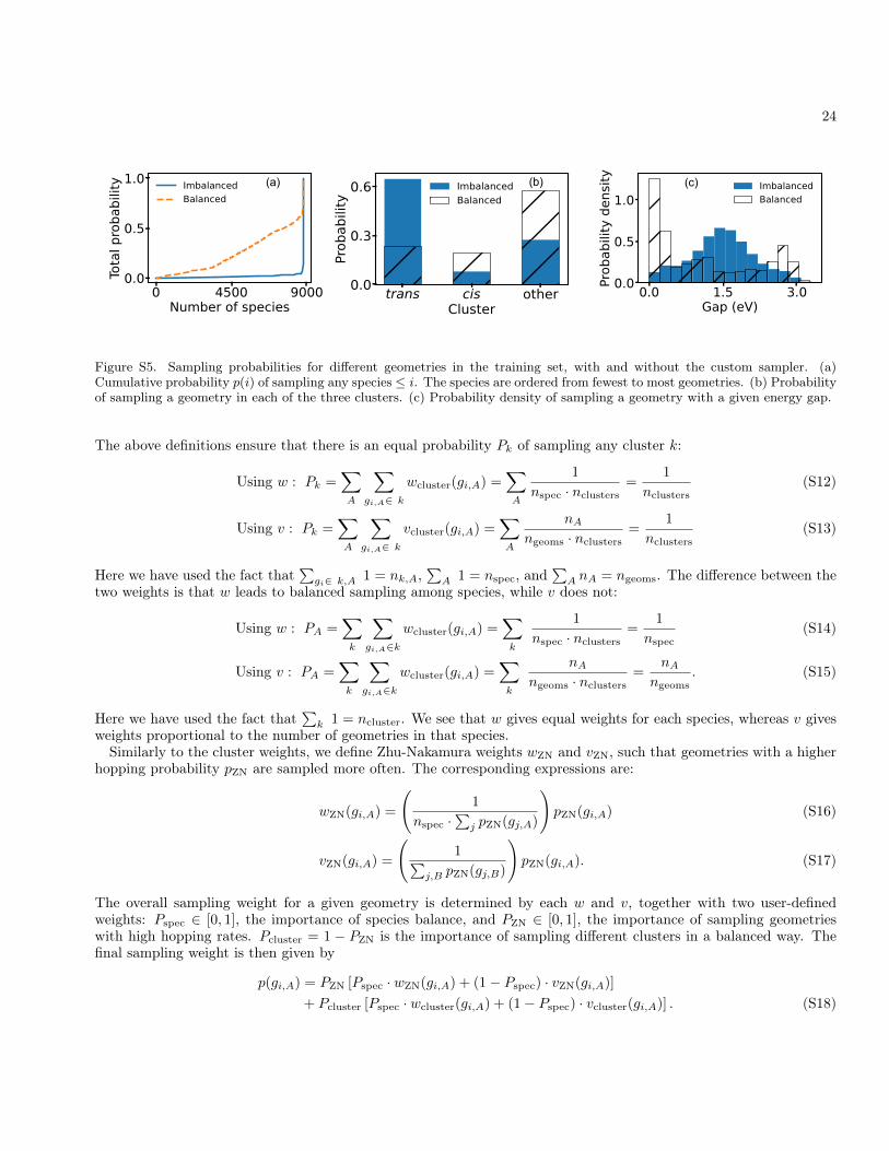
24

(c)(b)(a)

Figure S5. Sampling probabilities for different geometries in the training set, with and without the custom sampler. (a)Cumulative probability p(i) of sampling any species ≤ i. The species are ordered from fewest to most geometries. (b) Probabilityof sampling a geometry in each of the three clusters. (c) Probability density of sampling a geometry with a given energy gap.

The above definitions ensure that there is an equal probability Pk of sampling any cluster k:

Using w : Pk =∑A

∑gi,A∈ k

wcluster(gi,A) =∑A

1

nspec · nclusters=

1

nclusters(S12)

Using v : Pk =∑A

∑gi,A∈ k

vcluster(gi,A) =∑A

nAngeoms · nclusters

=1

nclusters(S13)

Here we have used the fact that∑

gi∈ k,A 1 = nk,A,∑

A 1 = nspec, and∑

A nA = ngeoms. The difference between thetwo weights is that w leads to balanced sampling among species, while v does not:

Using w : PA =∑k

∑gi,A∈k

wcluster(gi,A) =∑k

1

nspec · nclusters=

1

nspec(S14)

Using v : PA =∑k

∑gi,A∈k

wcluster(gi,A) =∑k

nAngeoms · nclusters

=nA

ngeoms. (S15)

Here we have used the fact that∑

k 1 = ncluster. We see that w gives equal weights for each species, whereas v givesweights proportional to the number of geometries in that species.

Similarly to the cluster weights, we define Zhu-Nakamura weights wZN and vZN, such that geometries with a higherhopping probability pZN are sampled more often. The corresponding expressions are:

wZN(gi,A) =

(1

nspec ·∑

j pZN(gj,A)

)pZN(gi,A) (S16)

vZN(gi,A) =

(1∑

j,B pZN(gj,B)

)pZN(gi,A). (S17)

The overall sampling weight for a given geometry is determined by each w and v, together with two user-definedweights: Pspec ∈ [0, 1], the importance of species balance, and PZN ∈ [0, 1], the importance of sampling geometrieswith high hopping rates. Pcluster = 1 − PZN is the importance of sampling different clusters in a balanced way. Thefinal sampling weight is then given by

p(gi,A) = PZN [Pspec · wZN(gi,A) + (1− Pspec) · vZN(gi,A)]

+ Pcluster [Pspec · wcluster(gi,A) + (1− Pspec) · vcluster(gi,A)] . (S18)

25

In applying Eq. (S18) we used Pspec = 0.6 and Pcluster = 0.5. We defined a geometry as cis or trans if its RMSDwith respect to the corresponding reference structure was ≤ 0.25 Å, and “other” otherwise. In contrast to diabaticreference geometries, the RMSD was computed using all atoms, not just the central CNNC atoms. Note that whileour clustering approach was specific to cis-trans isomerization, many black-box clustering methods exist, such ashierarchical clustering [45]. Any of these methods could have been used in place of our user-defined clusters.

In principle pZN should depend on trajectory-specific factors such as velocity, and is therefore not a function ofgeometry alone. However, during simulations, hops almost always occurred below 0.5 eV. Further, since pZN isapproximately exponential in the square of the gap, we approximated it with

pZN(∆E) ≈ exp(−∆E2/(2∆E20)), (S19)

where ∆E is the energy gap and ∆E0 = 0.15 eV. This choice of ∆E0 gave p(∆E = 0.5 eV) ≈ 3 × 10−3. This meantthat geometries were usually selected only if their gap was under 0.5 eV.

The sampling probabilities for the training set are shown in Fig. S5. Panel (a) shows the cumulative probability ofsampling different species, with the compounds ordered from fewest to most geometries. Without the custom samplerthe probability was quite small for most molecules. This was because the majority were combinatorially generatedand had few geometries. 90% of the probability was contained in the last 41 species. This probability was reducedto 35% when using the balanced sampler. Panel (b) shows that most geometries were trans isomers and few werecis. The custom sampler gave approximately equal probability to the two isomers, and the highest probability to theother group. Most geometries in this group had small gaps, and hence were highly weighted by wZN and vZN. This isdemonstrated in panel (c), which shows that near-CI geometries had the highest probabilities when using the balancedsampler.

7. Dynamics

Simulations were performed in two stages. First the starting geometries and velocities were generated for eachNAMD trajectory. For ab initio simulations we optimized the ground state geometry of each species and computedits normal modes. These modes were used to sample geometries and velocities from the harmonic oscillator Wignerdistribution at temperature T = 300 K [67]. For neural trajectories we ran classical MD for 15 ps with the Nosé-Hooverthermostat [48, 49], and selected random samples to start the NAMD trajectories. Classical MD was implementedwith ASE [68]. The effective mass Q was set to (3N − 6) · τ2kBT , where N is the number of atoms, kB is Boltzmann’sconstant, T = 300 K, and τ = 25 fs is the relaxation time. Initial atomic velocities were sampled from a Maxwell-Boltzmann distribution at 300 K. Optimized geometries were used for the initial atomic positions. The total linearand angular momenta of the system were set to zero, and the target kinetic energy was set to (3N − 6) · kBT/2. Thetime step of the simulation was set to 0.5 fs, and the neighbor list of the system was updated every 10 time steps(5 fs). All pairs of atoms within with 7 Å were considered neighbors. In each step the distance between all pairs ofneighbors was computed, and only pairs within 5 Å of each other were used in the model. This procedure meant thatatoms entering the 5 Å cutoff between neighbor list updates would not be missed. All ground state and excited statetrajectories in this work were propagated with the velocity Verlet algorithm [69]. Frames for NAMD were taken onlyafter the first 1 ps of ground state MD to allow for equilibration.

Next we ran ZN dynamics [26, 50, 70] using Ntrj trajectories, where Ntrj was 10 during the active learning cycle and500 during final inference. Hops were restricted to gaps ≤ 0.5 eV to avoid unphysical transitions, the time step wasset to 0.5 fs [26, 50, 70], and the neighbor list was again updated every 10 steps. Excited state trajectories were runfor 1.5 ps during active learning and 5 ps for final inference. All other details of the implementation can be found inRefs. [26, 50, 70]. For each species we performed inference in parallel over 100-250 geometries at a time, depending onthe number of atoms in the molecule. This was done by batching together geometries from 100-250 trajectories andevaluating the model on the batch. The batch size depended on the size of the molecule, which determined the GPUmemory consumption. FS simulations were also performed for final inference. The ZN parameters above were usedfor FS NN-NAMD of molecules in the holdout set. For virtual screening we used 100 trajectories and 2 ps of excitedstate dynamics. Species with a hopping rate under 10%, or with molecular graphs that changed during ground statedynamics, were deemed unreliable. These molecules were excluded from Fig. 4, but not from the average hoppingpercentage reported in the main text.

26

The quantum yield was calculated as Y = nR/nT ±√

(nT − nR)/(nT · nR), where nR is the number of reactivetrajectories and nT is the total number of trajectories [26]. To identify reactivity, we computed the RMSD betweenthe CNNC atoms in the final frame and the corresponding atoms in the optimized cis/trans geometries. A trajectorywas considered reactive if it started as cis and ended closer to trans, or vice-versa. Trajectories that ended in theexcited state were excluded from nR and nT . The yield was reported as 0 ± 0 if all trajectories ended in the excitedstate.

8. Neural network FS surface hopping

Tully’s surface hopping propagates the nuclei on one electronic surface at a time, called the active surface. Theexpansion coefficients of the electronic wavefunction are also propagated, and are used to make stochastic changes inthe active surface. The coefficient vector c, expressed in a basis denoted by “rep”, evolves as [71]

d

dtcrep = − i

~[Hrep − iTrep]crep. (S20)

The Hamiltonian matrix is Hrep = 〈ψrepn |H |ψrep

m 〉, and the coupling term is

(Trep)nm =

⟨ψrepn (~R(t))

∣∣∣∣ ∂∂t∣∣∣∣ψrep

m (~R(t))

⟩= ~v · ~krep

nm, (S21)

where ~v is the classical velocity of the nuclei. In principle the nuclei can be propagated on a PES in any electronic basis,and hops can be performed between states in that basis. For example, nuclei could be propagated on diabatic PESsand hops could occur between diabatic states. However, it is well-established that surface hopping in the adiabaticbasis gives the best results [61]. Hence the nuclei should be propagated in the adiabatic basis, and hops should bedecided using cad.

While the adiabatic basis should be used for hopping, c can be propagated in the diabatic basis, and then transformedinto the adiabatic basis for all subsequent manipulations (e.g. deciding on hops, adding decoherence, etc.). Indeed,using Eq. (S20) in the adiabatic basis can require small time steps for so-called trivial crossings, where derivativeNACVs are quite narrow and large [72]. Since global diabatic states are almost never available in ab initio simulations,a local diabatization method is often used to propagate c [52, 72]. This method is very stable and can be used witha fairly large time step. In this work we have a global diabatic basis that can replace local diabatization. FollowingRefs. [71, 72], we then propagate c as follows:

cad(t+ ∆t) = Pad(t, t+ ∆t)cad(t), (S22)

Pad(t, t+ ∆t) = U†(t+ ∆t)Pd(t, t+ ∆t)U(t) (S23)

Pd(t, t+ ∆t) = ΠKk=1 exp

[−iHd

k∆t/K]

(S24)

Hdk = Hd(t) +

k

K

[Hd(t+ ∆t)−Hd(t)

]. (S25)

Here Pad(t, t + ∆t) is the propagator of cad from t to t + ∆t (Eq. (S22)), and ∆t is the timestep. The adiabaticpropagator is a transformation of the diabatic propagator into the adiabatic basis (Eq. (S23)), using the transformationmatrix U (Eq. (2)). The diabatic propagator is a matrix product of K sub-propagators (Eq. (S24)), where Kis the number of electronic substeps for each nuclear step. “exp” denotes a matrix exponential, not element-wiseexponentiation. The kth sub-propagator uses a linear interpolation between Hd(t) and Hd(t + ∆t) to approximateHd(t+ k∆t/K) (Eq. (S25)). The diabatic Hamiltonian is produced by the neural network model. The probability ofhopping from state n to m is [71]

pn→m =

(1− |c

adn (t+ ∆t)|2

|cadn (t)|2

) Re[cadm (t+ ∆t)

(P admn

)∗ (cadn (t)

)∗]|cad

n (t)|2 − Re[cadn (t+ ∆t) (P ad

nn)∗

(cadn (t))

∗] , (S26)

27

where Re(x) is the real part of x.In this work we initialized cad(t = 0) = [0, 1, 0], used Eqs. (S22)-(S25) to generate cad(t + ∆t), and computed the

hopping probability with Eq. (S26). cad was expressed in a three-state basis because our model used three diabaticstates, and hence U had three dimensions. Since the model was only trained on the first and second adiabatic energies,we set p = 0 for all transitions to the third state. Hops to state m were performed if [71]

m−1∑i=1

pn→i < r ≤m−1∑i=1

pn→i + pn→m, (S27)

where 0 ≤ r ≤ 1 is a random number. The momentum was rescaled after each hop to conserve the total energy. Themomentum was multiplied by a constant factor, rather than being re-scaled in the direction of the NACV, to avoidthe overhead of a NACV calculation (see below) [52]. If the factor was complex—a so-called “frustrated” hop—thenno transition was made [52].

We also tested propagation in the adiabatic basis. In this case we used the NACV to evaluate T, and constructedP ad from the interpolation of Had − iT [71]. Both Eq. (S26) and Tully’s original hopping expression [25] wereused. The momentum was re-scaled in the direction of the NACV [73]. In all cases the results were very similar tothose of the diabatic basis. Diabatic propagation was ultimately chosen because of its reported stability [72], andbecause of its computational efficiency. In particular, the diabatic propagation requires only diabatic energies andone adiabatic gradient. It therefore uses only one forward and one backward pass through the neural network. Bycontrast, constructing the NACVs requires gradients for each diabatic element (Eq. (1)). For three diabatic states,this corresponds to one forward pass and six backward passes. While shared convolution layers and caching mean thatN gradients do not take N× as long as one gradient, we found that they still added significant time. Hence diabaticpropagation was chosen as the most efficient method.

The decoherence correction of Ref. [74] was used to counter the over-coherence of Tully’s original method. A signcorrection was also used to remove random sign changes in the eigenvectors of Hd. The sign correction Am for themth eigenvector vm was computed as

Am = sgn(Sn′m) (S28)

Snm = v†n(t)vm(t+ ∆t) = [U†(t)U(t+ ∆t)]nm (S29)n′ = argmaxn{|Snm|}. (S30)

The transformation matrix and NACVs were corrected through

Unm(t+ ∆t)→ AmUnm(t+ ∆t) (S31)~knm(t+ ∆t)→ AnAm

~knm(t+ ∆t) (S32)~gnm(t+ ∆t)→ AnAm~gnm(t+ ∆t). (S33)

Note also that Snm ≈⟨ψadn (t)

∣∣ψadm (t+ ∆t)

⟩:⟨

ψadn (t)

∣∣ψadm (t+ ∆t)

⟩=∑ij

U∗in(t)Ujm(t+ ∆t)⟨ψdi (t)

∣∣ψdj (t+ ∆t)

⟩≈∑ij

U†ni(t)Ujm(t+ ∆t)⟨ψdi (t)

∣∣ [(1− (~v∆t) · ∇R)∣∣ψd

j (t)⟩]

=∑ij

U†ni(t)Ujm(t+ ∆t)⟨ψdn(t)

∣∣ψdm(t)

⟩= [U†(t)U(t+ ∆t)]nm = Snm. (S34)

Here we used the fact that there is no derivative coupling between diabatic states, and that the diabatic states at agiven time are orthonormal (Eq. (S40)).

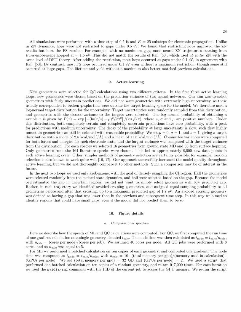
28

All simulations were performed with a time step of 0.5 fs and K = 25 substeps for electronic propagation. Unlikein ZN dynamics, hops were not restricted to gaps under 0.5 eV. We found that restricting hops improved the ZNresults but hurt the FS results. For example, with no maximum gap, most neural ZN trajectories starting fromtrans-azobenzene hopped at ∼ 1.5 eV. This did not match the results of Ref. [50], which used ab initio ZN with thesame level of DFT theory. After adding the restriction, most hops occurred at gaps under 0.1 eV, in agreement withRef. [50]. By contrast, most FS hops occurred under 0.1 eV even without a maximum restriction, though some stilloccurred at large gaps. The lifetime and yield without a maximum also better matched previous calculations.

9. Active learning

New geometries were selected for QC calculations using two different criteria. In the first three active learningloops, new geometries were chosen based on the prediction variance of two neural networks. Our aim was to selectgeometries with fairly uncertain predictions. We did not want geometries with extremely high uncertainty, as theseusually corresponded to broken graphs that were outside the target learning space for the model. We therefore used alog-normal target distribution for the uncertainty. Target uncertainties were randomly sampled from this distribution,and geometries with the closest variance to the targets were selected. The log-normal probability of obtaining asample x is given by P (x) = exp

[−(ln(x/s)− µ)2/2σ2

]/(xσ

√2π), where s, σ and µ are positive numbers. Under

this distribution, both completely certain and completely uncertain predictions have zero probability, with a peakfor predictions with medium uncertainty. The decay of the probability at large uncertainty is slow, such that highlyuncertain geometries can still be selected with reasonable probability. We set µ = 0, σ = 1, and s = 7, giving a targetdistribution with a mode of 2.5 kcal/mol(/Å) and a mean of 11.5 kcal/mol(/Å). Committee variances were computedfor both forces and energies for each electronic state, and the largest variance was compared with the target variancefrom the distribution. For each species we selected 16 geometries from ground state MD and 33 from surface hopping.Only geometries from the 164 literature species were chosen. This led to approximately 8,000 new data points ineach active learning cycle. Other, simpler methods of geometry selection are certainly possible; for example, randomselection is also known to work quite well [16, 17]. Our approach successfully increased the model quality throughoutactive learning, but we did not thoroughly compare it to other methods. Such a comparison may be of interest in thefuture.

In the next two loops we used only azobenzene, with the goal of densely sampling the CI region. Half the geometrieswere selected randomly from the excited state dynamics, and half were selected based on the gap. Because the modeloverestimated the gap in uncertain regions, we did not want to simply select geometries with low predicted gap.Rather, in each trajectory we identified avoided crossing geometries, and assigned equal sampling probability to allgeometries before and after that crossing, up to a maximum predicted gap of 1.7 eV. An avoided crossing geometrywas defined as having a gap that was lower than in the previous and subsequent time step. In this way we aimed toidentify regions that could have small gaps, even if the model did not predict them to be so.

10. Figure details

a. Computational speed-up

Here we describe how the speeds of ML and QC calculations were computed. For QC, we first computed the run timeof one gradient calculation on a single geometry, denoted tcalc. The node time was then calculated as tnode = tcalc/ncalc,with ncalc = (cores per node)/(cores per job). We assumed 40 cores per node. All QC jobs were performed with 8cores, and so ncalc was equal to 5.

For ML we performed a batched calculation on ten copies of each geometry, and computed one gradient. The nodetime was computed as tnode = tcalc/ncalc, with ncalc = 10 · (total memory per gpu)/(memory used in calculation) ·(GPUs per node). We set (total memory per gpu) = 32 GB and (GPUs per node) = 2. We used a script thatperformed one batched calculation on ten copies of a random geometry, and re-ran it 7,000 times. For each iterationwe used the nvidia-smi command with the PID of the current job to access the GPU memory. We re-ran the script

29

many times, rather than running many calculations in one script, because nvidia-smi does not account for all freedmemory until a job is finished. That is, after one calculation is finished, nvidia-smi shows that GPU memory is stillbeing occupied by the job. This occurs even after all local variables are deleted. Hence running multiple calculationsin one script would yield an overestimated GPU memory.

In the above calculation, we implicitly assumed that multiplying the batch size by x would lead to an x-fold increasein memory. In practice we have found that the memory is increased by less than that. This means that the MLspeedup in Fig. 3 is a conservative estimate.

b. Diabatic energies

Since three diabatic states were used in the DANN model, and since all three were coupled near the CI, it wouldbe incorrect to plot only two states in Fig. 3(b). We therefore applied a fixed rotation matrix, U 6= U(~R), togenerate a new diabatic Hamiltonian with only two coupled states. The new diabatic Hamiltonian was given byH′d(~R) = U†Hd(~R)U. Note that any position-independent rotation matrix can be brought outside the gradientin Eq. (1), and so H′d is still diabatic. The rotation matrix was chosen to diagonalize Hd at the CI, so thatU†Hd(~RCI)U = diag({E}). This led to d′00 = d′11 and d′01 = 0 at the CI. Hence the lowest two rotated states werethe most important contributors to E0 and E1, and were therefore used in Fig. 3(b).

11. Intensive and extensive quantities

The DANN model predicts each property by summing over atomic contributions, just as in the PaiNN model.This guarantees size-extensivity. However, as explained below, the off-diagonal elements of Hd should be intensive,in the sense that atoms not involved in the excitation should not contribute to these values. Nonetheless, we foundthat summation for these terms gave better results than averaging. This was true even when using a learnableweighted average. Atom-wise summation can still generate accurate dnm, because the readout network can simplymap unimportant atoms to zero.

To demonstrate extensivity and intensivity, consider two uncoupled subsystems, A and B. The total clampednucleus Hamiltonian is H(~r, ~R) = HA(~r, ~R) +HB(~r, ~R). Let the excitation of interest be in subsystem A. In this casethe adiabatic states involve only excitations in subsystem A, so that the nth diabatic wave function is written as

ψd,n(~r; ~R) = ψBad,0(~r; ~R)

∑k

UnkψAad,k(~r; ~R). (S35)

The diabatic state is a direct product of the ground state wave function of system B, ψBad,0(~r; ~R), and a rotation of

the adiabatic states of system A, ψAad,k(~r; ~R). The matrix elements of Hd are then given by

(Hd)nm = 〈ψd,n|H(~r, ~R)|ψd,m〉

=∑kl

U∗nkUml〈ψBad,0ψ

Aad,k| HA(~r, ~R) +HB(~r, ~R) |ψB

ad,0ψAad,l〉

=∑kl

U∗nkUml

(Ek,A + EB

)δkl

=∑k

U∗inUmkEk,A + EB

(UU†

)mn

= HAd,nm + EB δnm. (S36)

Hence the diagonal elements of Hd each gain the adiabatic energy of B, while the off-diagonal elements remain thesame. To understand this result physically, consider that adding a scalar multiplied by the identity yields eigenvaluesthat are each shifted by the scalar. This means that the eigenvalues of Hd are each shifted by EB . Therefore the

30

excitation energy is unchanged, which is the expected behavior upon adding an uncoupled system. Note also thatextensivity is sometimes described as doubling the energy when the system size is doubled. However, this definition istoo narrow, as it applies to only one adiabatic energy at a time. For example, if subsystem B is a copy of subsystem A,then EB = E0,A, meaning that E0 = E0,A +EB = 2E0,A, and so the ground state energy is indeed doubled. However,E1 = E1,A +EB = 2E1,A−gap, where gap = E1,A−E0,A. Therefore, the excited state energy is not doubled. A moregeneral definition is that the energy of the second subsystem is added to each adiabatic energy.

This analysis shows that the off-diagonal elements of Hd are intensive. The adiabatic energy gap is also intensive.Intensive here means that adding a subsystem that does not participate in the excitation does not modify the quantity.Such properties can naturally be modeled with an attention mechanism [75–78] that learns the importance of each atomto the excitation. For example, the excitation energy can be modeled as an attention-weighted sum over atomwisequantities. However, as discussed in Supplementary Sec. 5, this approach led to worse performance than simplypredicting extensive energies for each state.

12. Proof of diabaticity

Here we prove Eq. (1) in the main text. Using bra-ket notation for the wave functions, we define the diabatic statesas a linear combination of adiabatic states,

|ψd,n〉 =∑m

|ψad,m〉V ∗nm, (S37)

where V is a unitary matrix. Multiplying each side by Vnn′ and summing over n yields

|ψad,n〉 =∑m

|ψd,m〉Vmn, (S38)

where we have renamed the dummy indices, n→ m and n′ → n. We have also used the fact that (V†V)nm = δnm forany unitary matrix, where δnm is the Kronecker delta. Given the connection between diabatic and adiabatic states,we can relate V to the derivative coupling ~k:

~knm ≡ 〈ψad,n| ∇R |ψad,m〉

=∑ij

V ∗jn (∇RVim 〈ψd,j |ψd,i〉+ Vim 〈ψd,j | ∇R |ψd,i〉)

=∑i

V ∗in∇RVim. (S39)

We have used the fact that, by definition, the derivative coupling between any two diabatic states is zero. We havealso used the orthonormality of the diabatic states:

〈ψd,j |ψd,i〉 =∑nm

VjnV∗im 〈ψad,n|ψad,m〉 =

∑nm

VjnV∗imδnm =

(VV†

)ij

= δij , (S40)

which follows from the orthonormality of the adiabatic wave functions. Meanwhile, by construction, the Hamiltonianproduced by the model has eigenvalues equal to the adiabatic energies:

(Hd)nm =(Udiag({E})U†

)nm

=∑ij

Uni (Eiδij)U∗mj

=

(∑i

Uni 〈ψad,i|

)H

∑j

U∗mj |ψad,j〉

, (S41)

31

where U is the unitary matrix that diagonalizes Hd, H is the Hamiltonian operator, and we have used the relation〈ψad,j | H |ψad,i〉 = Ei 〈ψad,j |ψad,i〉 = Eiδij . Comparing Eqs. (S41) and (S37), we see that Hd is the representation ofH in a different electronic basis. In particular, if we choose U = V, such that U satisfies Eq. (S39), then Hd is therepresentation of H in the diabatic basis.

The model could be trained directly with Eq. (S39). However, the equation is numerically ill-posed because ~knmdiverges at conical intersections. It is preferable to work instead with the force coupling, ~gnm. We now show that Eq.(1), which is defined in terms of ~gnm, holds only if (S39) is satisfied. The left-hand side of Eq. (1) can be written as∑

ij

U∗in∇R

(Udiag({E})U†

)ijUjm

=∑ijk

U∗in[(∇REk)UikU

∗jk + Ek (∇RUik)U∗jk + Ek Uik(∇RU

∗jk)]Ujm. (S42)

The first term is ∑k

(U†U)nk (∇REk) (U†U)km = (∇REn)δnm, (S43)

where we have used the fact that (U†U)nm = δnm. Substituting Eq. (S39) with V = U, the second term is∑k

~knk(U†U)kmEk = ~knmEm. (S44)

Performing the same substitution for the third term gives∑k

~k∗mk(U†U)nkEk = −~knmEn, (S45)

where we have used the anti-Hermitian property ~k∗mn = −~knm. Adding the three terms gives

(U†(∇RHd)U

)nm

=

{∇REn, if n = m,

(Em − En)~knm, if n 6= m.(S46)

Noting that ~fn = −∇REn and ~gnm = (Em − En)~knm gives Eq. (1) in the main text. Hence Eq. (1) can only holdif Eq. (S39) is true. Therefore, enforcing Eq. (1) ensures that there is no derivative coupling between any pair ofdiabatic states. Note that in the main text we used three diabatic states, and trained only on energies and couplingsbetween the first two adiabatic states. This still means that all three diabatic states are properly diabatic: if Eq. (1)is satisfied for even one pair of adiabatic states, then the derivative coupling must be zero between all pairs of diabaticstates.

32

13. Training species

Here we provide the motifs and substituents used for combinatorial molecule generation, together with a list of theliterature species used for dense configurational sampling. Species with a net charge were excluded from training butare given here for completeness. In some cases only the cis or trans isomer was actually investigated experimentally,but in all cases we reference the publication for both isomers.

Many species in both the training and test set had experimental S1 yields in non-polar solution. We did not put allsuch molecules in the test set, because this would mean losing hundreds of thousands of training geometries. Insteadwe used the 40 species with the fewest QC calculations.

Table S6. Motifs used for combinatorial species generation. Examples of literature species for each motif are also given. Thespecies numbers are those in Tables S8 and S9.

Graphs Literature species

NN

X

X

NN XX

1, 2, 25, 26, 63, 64, 125, 126

NN

X

Y

NN

Y X

19, 20, 27, 28, 37, 38, 39, 40, 61, 62, 69, 70, 73, 74, 75, 76, 83, 84, 97,98, 115, 116, 117, 118, 119, 120, 121, 122, 123, 124, 127, 128, 129, 130,

147, 148, 155, 156, 157, 158, 163, 164

NN

Y

Y X

X

NN

Y Y

X X

67, 68, 87, 88, 99, 100, 101, 102, 103, 104, 105, 106, 107, 108

NN

Y

Y X

X

X

X

NN

YY

XX

XX

9, 10, 13, 14, 15, 16, 17, 18, 21, 22, 95, 96, 131, 132, 133, 134, 135,136, 137, 138, 139, 140, 161, 162

33

Table S7. Substituents used for combinatorial species generation. “Azo” denotes the azobenzene attachment site.

SMILES Graph

[Azo]N(C)Cc1ccccn1 Azo

N

N

[Azo]N Azo NH2

[Azo]N(CC)Cc1ccccc1 Azo

N

[Azo]C(N)=OAzo NH2

O

[Azo]OCc1cc(OCc2ccccc2)cc(OCc2ccccc2)c1

AzoO

O

O

[Azo]N1CCCCC1Azo

N

[Azo]c1ccccc1Azo

[Azo]NC(=O)CCl AzoNH

O

Cl

[Azo]OC(C)=OAzo

O

O

[Azo]N1CCN(C(C)=O)CC1

AzoN

N

O

[Azo]NC(=O)C[N+](CC)(CC)CCAzo

NH

O

N+

[Azo]Cl Azo Cl

[Azo]COAzo OH

[Azo]C(=O)OCCAzo

O

O

[Azo]CCAzo

[Azo]C(=O)OAzo

O

OH

[Azo]C#C Azo

34

[Azo]NC(=O)CN1C(=O)C=CC1=O AzoNH

O

N

O

O

[Azo][N+](=O)[O-]Azo

N+

O

O-

[Azo][N+](C)(C)C Azo N+

[Azo]O Azo OH

[Azo]Oc1c(N)cccc1CC(C)CAzo

O

NH2

[Azo]F Azo F

[Azo]N1CCN(C(=O)CCl)CC1

AzoN

N

O

Cl

[Azo]Oc1c(N)cccc1C(C)CAzo

O

NH2

[Azo]NCc1ccccn1Azo

HN

N

[Azo]OCc1ccccc1Azo

O

[Azo]NC(C)=O AzoNH

O

[Azo]c1cn(-c2ccc3cc4ccccc4cc3c2)nn1 AzoN

N N

[Azo]C Azo

[Azo]C(=O)C(F)(F)FAzo

O

F

FF

[Azo]N1CCN(C)CC1Azo

N

N

[Azo]c1cn(-c2cccc3ccccc23)nn1

Azo

NN

N

35

[Azo]c1cn(-c2ccccc2)nn1 AzoN

N N

[Azo]C(C)C Azo

[Azo]C(=O)OCAzo

O

O

[Azo]N1CCOCC1Azo

N

O

[Azo]N(CC)c1ccccc1

Azo

N

[Azo]N(C)CAzo

N

[Azo]N1CCCC1 AzoN

[Azo]N1CC2CN(C(C)=O)CC2C1 AzoNN

O

[Azo]C(C)(C)CAzo

[Azo]NC(=O)C=C AzoNH

O

[Azo]N(CCCCCCCC)CCCCCCCC AzoN

[Azo]OCC AzoO

[Azo]N(CC)CC Azo

N

36

[Azo]N(c1ccc2c(c1)C(C)(C)c1ccccc1-2)c1ccc2c(c1)C(C)(C)c1ccccc1-2

Azo

N

[Azo]NC(=O)CCC[C@H](C[C@H](N)C(=O)O)C(=O)O Azo

NH

O NH2

O

OH

O OH

37

Table S8. Test set species and literature quantum yields. For papers that reported the yield at different wavelengths, we chosethe wavelength closest to the n− π∗ (S1) absorption maximum. Quantum yields computed with FS surface hopping using thediabatic model are also shown.

# SMILES Graph Ref. (S1 yield, solvent)

1c1ccc(CNc2ccccc2/N=N/c2ccccc2NCc2ccccn2)nc1

NH

NN

HN

N

N

[38]Exp: (02, many)

Calc: 0 ± 0

2c1ccc(CNc2ccccc2/N=N\c2ccccc2NCc2ccccn2)nc1

NH

N

N

HN

N

N

[38]Exp: None

Calc: 0.51 ± 0.04

3 c1ccc(/N=N/c2cccc3ccccc23)cc1 NN [79]

Exp: (0.25, methylcyclopentane)Calc: 0.43 ± 0.06

4 c1ccc(/N=N\c2cccc3ccccc23)cc1

NN

[79]

Exp: (0.49, methylcyclopentane)Calc: 0.57 ± 0.04

5

CC1(C)c2ccccc2-c2ccc(N(c3ccc(/N=N/c4ccccc4)cc3)c3ccc4c(c3)C(C)(C)

c3ccccc3-4)cc21N

N N

[80]Exp: (0.29, toluene)Calc: 0.19 ± 0.24

6

CC1(C)c2ccccc2-c2ccc(N(c3ccc(/N=N\c4ccccc4)cc3)c3ccc4c(c3)C(C)(C)

c3ccccc3-4)cc21 N

N N

[80]Exp: (0.31, toluene)Calc: 0.54 ± 0.04

38

7 Cc1cc(C)c(/N=N/c2ccccc2)c(C)c1 NN

[81]

Exp: (0.16,methylcyclohexane and

isohexane)Calc: 0.34 ± 0.07

8 Cc1cc(C)c(/N=N\c2ccccc2)c(C)c1N

N

[81]

Exp: (0.38,methylcyclohexane and

isohexane)Calc: 0.60 ± 0.04

9Cc1cc(C)c(/N=N/c2c(C)

cc(C)cc2C)c(C)c1 NN

[81,82]

Exp: (0.16-0.22,methylcyclohexane andisohexane) [81], (0.24,n-hexane) [82]Calc: 0.41 ± 0.05

10Cc1cc(C)c(/N=N\

c2c(C)cc(C)cc2C)c(C)c1

NN [81,

82]

Exp: (0.44,methylcyclohexane andisohexane) [81], (0.5,n-hexane) [82]Calc: 0.59 ± 0.04

11Cc1cc(/N=N/c2ccccc2N

(C)Cc2ccccn2)c(N(C)Cc2ccccn2)cc1O NN

N

N

N

N

OH

[39]Exp: (02, many)Calc: 0.33 ± 0.12

12Cc1cc(/N=N\c2ccccc2N

(C)Cc2ccccn2)c(N(C)Cc2ccccn2)cc1ON

N

NN

N

N

OH

[39]Exp: None

Calc: 0.53 ± 0.04

13CCc1cc(CC)c(/N=N/

c2c(CC)cc(CC)cc2CC)c(CC)c1 NN

[82]Exp: (0.25, n-hexane)

Calc: 0.32 ± 0.07

14CCc1cc(CC)c(/N=N\

c2c(CC)cc(CC)cc2CC)c(CC)c1N

N

[82]Exp: (0.5, n-hexane)

Calc: 0.50 ± 0.04

39

15CC(C)c1cc(C(C)C)c(/N=N/c2c(C

(C)C)cc(C(C)C)cc2C(C)C)c(C(C)C)c1 NN [82]

Exp: (0.19, n-hexane)Calc: 0.26 ± 0.07

16CC(C)c1cc(C(C)C)c(/N=N\c2c(C

(C)C)cc(C(C)C)cc2C(C)C)c(C(C)C)c1

N

N

[82]Exp: (0.55, n-hexane)

Calc: 0.53 ± 0.04

17

CC(C)(C)c1cc(C(C)(C)C)c(/N=N/c2c(C(C)(C)C)cc(C(C)(C)C)cc2C

(C)(C)C)c(C(C)(C)C)c1 NN [82]

Exp: (0, n-hexane)Calc: 0.01 ± 0.44

18

CC(C)(C)c1cc(C(C)(C)C)c(/N=N\c2c(C(C)(C)C)cc(C(C)(C)C)cc2C

(C)(C)C)c(C(C)(C)C)c1

N

N

[82]Exp: None

Calc: 0.78 ± 0.02

19CCCCCCCCN(CCCCCCCC)c1ccc

(/N=N/c2ccc(C(=O)C(F)(F)F)cc2)cc1

N

NN

OF

F

F

[83]Exp: (0.163, toluene)

Calc: 0.08 ± 0.55

20CCCCCCCCN(CCCCCCCC)c1ccc

(/N=N\c2ccc(C(=O)C(F)(F)F)cc2)cc1

N

NN

O

FF

F[83]

Exp: (0.7-13, toluene)Calc: 0.66 ± 0.03

21CCOC(=O)c1cc(F)c(/N=N/c2c(F)cc(C(=O)OCC)cc2F)c(F)c1

O

O

F

NN

F

O

OF

F

[84]Exp: (0.1, hexane)Calc: 0.08 ± 0.20

40

22CCOC(=O)c1cc(F)c(/N=N\c2c(F)cc(C(=O)OCC)cc2F)c(F)c1

O

O

F

NN

F

OO

F F

[84]Exp: (0.53, hexane)Calc: 0.44 ± 0.05

23CC(=O)Oc1cc(N(C)Cc2ccccn2)c

(/N=N/c2ccccc2N(C)Cc2ccccn2)cc1C O

ONN

NN

NN

[39]Exp: (0.17, C6D6)Calc: 0.30 ± 0.13

24CC(=O)Oc1cc(N(C)Cc2ccccn2)c

(/N=N\c2ccccc2N(C)Cc2ccccn2)cc1CO

ONN

N

N

N

N

[39]Exp: None

Calc: 0.50 ± 0.04

25CN(Cc1ccccn1)c1ccccc1

/N=N/c1ccccc1N(C)Cc1ccccn1

N

N

NN

N

N

[38]Exp: (0.19, CDCl3)Calc: 0.37 ± 0.08

26CN(Cc1ccccn1)c1ccccc1

/N=N\c1ccccc1N(C)Cc1ccccn1

N

N

N

N

NN

[38]Exp: None

Calc: 0.48 ± 0.04

27COc1ccc(/N=N/c2ccc([N+](=O)[O-])cc2)cc1

O

NN

N+

O

O-

[81]

Exp: (0.17,methylcyclohexane and

isohexane)Calc: 0.05 ± 0.43

28COc1ccc(/N=N\c2ccc([N+](=O)[O-])cc2)cc1

O

NN

N+

O

O-

[81]

Exp: (0.55,methylcyclohexane and

isohexane)Calc: 0.46 ± 0.05

41

29COc1cc(N(C)Cc2ccccn2)

c(/N=N/c2ccccc2N(C)Cc2ccccn2)cc1C

ONN

NN

NN

[39]Exp: (02, many)Calc: 0.13 ± 0.31

30COc1cc(N(C)Cc2ccccn2)

c(/N=N\c2ccccc2N(C)Cc2ccccn2)cc1C

ONN

N

N

N

N

[39]Exp: None

Calc: 0.54 ± 0.04

31 Fc1cccc(F)c1/N=N/c1ccccc1

F

F

NN [84]

Exp: (0.32, hexane)Calc: 0.39 ± 0.06

32 Fc1cccc(F)c1/N=N\c1ccccc1F

F

N

N [84]Exp: (0.55, hexane)Calc: 0.53 ± 0.04

33Fc1cccc(F)c1/N=N/c1c(F)cc(-

c2ccccc2)cc1F

F

F

NN

F

F

[85]Exp: (0.15, n-hexane)

Calc: 0.41 ± 0.06

34Fc1cccc(F)c1/N=N\c1c(F)cc(-

c2ccccc2)cc1FFF

NN

F

F

[85]Exp: (0.28, n-hexane)

Calc: 0.51 ± 0.04

35 Nc1ccccc1/N=N/c1ccccc1NCc1ccccn1

H2N

NN

HN

N

[38]Exp: (02, many)Calc: 0.04 ± 0.98

36 Nc1ccccc1/N=N\c1ccccc1NCc1ccccn1

NH2

N

N

NH

N

[38]Exp: None

Calc: 0.54 ± 0.04

42

37OCc1ccc(/N=N/c2ccc(OCc3ccccc3)cc2)cc1

OH

NN

O

[86]

Exp: (0.4,dichloromethane)Calc: 0.13 ± 0.23

38OCc1ccc(/N=N\c2ccc(OCc3ccccc3)cc2)cc1

OH

NN

O [86]

Exp: (0.61,dichloromethane)Calc: 0.53 ± 0.04

39

OCc1ccc(/N=N/c2ccc(OCc3cc(OCc4ccccc4)cc(OCc4ccccc4)c3)cc2)cc1

OH

NN

O

O

O

[86]

Exp: (0.36,dichloromethane)Calc: 0.13 ± 0.24

40

OCc1ccc(/N=N\c2ccc(OCc3cc(OCc4ccccc4)cc(OCc4ccccc4)c3)cc2)cc1

OH

NN

O

O

O

[86]

Exp: (0.64,dichloromethane)Calc: 0.54 ± 0.04

2 In Refs. [38, 39], the non-reactive azobenzene derivatives wereirradiated from 300 to 600 nm. This range covered both S0 → S1

and S0 → S2 excitation. Only small changes in absorbance wereobserved, indicating minimal trans→cis isomerization. However,the S2 transition was highly redshifted, and thus had significantoverlap with the S1 transition. The S2 transition also had a much

higher oscillator strength. Hence the small absorbance changescould have been due to the S1 transition, and so the S1 yieldmay not have been precisely 0. The S1 yield should therefore beinterpreted as “small”, rather than exactly zero.

3 Averaged over excitations at 313, 436, and 546 nm.

43

Table S9. Training and validation set literature species used for dense configurational sampling.

# SMILES Graph Ref.

41 c1ccc2c(c1)CCc1ccccc1/N=N/2NN

[87]

42 c1ccc2c(c1)CCc1ccccc1/N=N\2N N

[87]

45 c1ccc2c(c1)COc1ccccc1/N=N/2O

NN

[88]

46 c1ccc2c(c1)COc1ccccc1/N=N\2O

N N

[88]

47 c1ccc2c(c1)CSc1ccccc1/N=N/2S

NN

[88]

48 c1ccc2c(c1)CSc1ccccc1/N=N\2S

N N

[88]

49 c1ccc2cc(/N=N/c3ccc4ccccc4c3)ccc2c1N

N [79]

50 c1ccc2cc(/N=N\c3ccc4ccccc4c3)ccc2c1

NN

[79]

51 c1ccc(/N=N/c2ccccc2)cc1 NN

[81, 82, 85,89–92]

52 c1ccc(/N=N\c2ccccc2)cc1

NN [81, 82, 85,

89–92]

53CC1(C)c2cccc(N)c2Oc2c(/N=N/

c3cccc4c3Oc3c(N)cccc3C4(C)C)cccc21 NH2

O

NN

O

NH2 [93]

44

54CC1(C)c2cccc(N)c2Oc2c(/N=N\

c3cccc4c3Oc3c(N)cccc3C4(C)C)cccc21 NH2

O

NN

O

NH2

[93]

55 Cc1cccc(C)c1/N=N/c1c(C)cccc1C NN

[94]

56 Cc1cccc(C)c1/N=N\c1c(C)cccc1C

NN

[94]

57 Cc1cccc(C)c1/N=N/c1ccc(C(=O)O)cc1NN

O

OH[95]

58 Cc1cccc(C)c1/N=N\c1ccc(C(=O)O)cc1

N

N

O OH

[95]

59 Cc1ccc(/N=N/c2ccccc2)cc1N

N [89]

60 Cc1ccc(/N=N\c2ccccc2)cc1

NN

[89]

61 Cc1ccc(/N=N/c2ccc(C)cc2)cc1N

N [89]

62 Cc1ccc(/N=N\c2ccc(C)cc2)cc1

NN

[89]

63 CCc1ccccc1/N=N/c1ccccc1CC NN

[94]

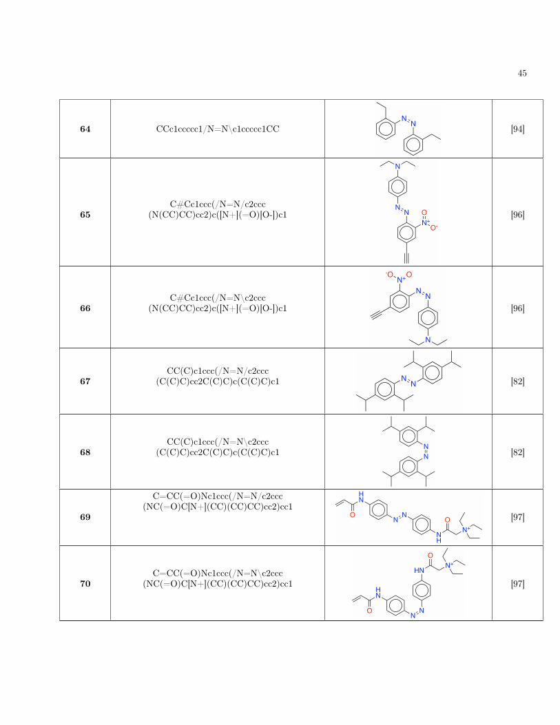
45

64 CCc1ccccc1/N=N\c1ccccc1CCNN [94]

65C#Cc1ccc(/N=N/c2ccc

(N(CC)CC)cc2)c([N+](=O)[O-])c1 NN

N

N+

O

O-

[96]

66C#Cc1ccc(/N=N\c2ccc

(N(CC)CC)cc2)c([N+](=O)[O-])c1

NN

N

N+O-O

[96]

67CC(C)c1ccc(/N=N/c2ccc

(C(C)C)cc2C(C)C)c(C(C)C)c1 NN [82]

68CC(C)c1ccc(/N=N\c2ccc

(C(C)C)cc2C(C)C)c(C(C)C)c1N

N[82]

69

C=CC(=O)Nc1ccc(/N=N/c2ccc(NC(=O)C[N+](CC)(CC)CC)cc2)cc1

O

HN

NN

NH

O

N+

[97]

70C=CC(=O)Nc1ccc(/N=N\c2ccc

(NC(=O)C[N+](CC)(CC)CC)cc2)cc1

O

HN

NN

HN

O

N+

[97]

46

71 CCN1Cc2ccccc2/N=N/c2ccccc21 N

NN

[88]

72 CCN1Cc2ccccc2/N=N\c2ccccc21N

NN

[88]

73CCN(c1ccccc1)c1ccc(/N=N/

c2ccc(NC(=O)C[N+](CC)(CC)CC)cc2)cc1N

NN

NH

O

N+

[97]

74CCN(c1ccccc1)c1ccc(/N=N\

c2ccc(NC(=O)C[N+](CC)(CC)CC)cc2)cc1

N

NN

HN

O

N+

[97]

75CCN(Cc1ccccc1)c1ccc(/N=N/

c2ccc(NC(=O)C[N+](CC)(CC)CC)cc2)cc1

N

NN

NH

O

N+

[97]

76CCN(Cc1ccccc1)c1ccc(/N=N\

c2ccc(NC(=O)C[N+](CC)(CC)CC)cc2)cc1

N

NN

HN

O

N+[97]

47

77

CCN(CC)c1ccc(/N=N/c2ccc(-c3cn(-c4ccc5cc6ccccc6cc5c4)nn3)cc2

[N+](=O)[O-])cc1

N

NN

N N

N

N+O

-O

[96]

78

CCN(CC)c1ccc(/N=N\c2ccc(-c3cn(-c4ccc5cc6ccccc6cc5c4)nn3)cc2

[N+](=O)[O-])cc1

N

N

NN

N N

N+

O

O-

[96]

79CCN(CC)c1ccc(/N=N/c2ccc(-c3cn

(-c4cccc5ccccc45)nn3)cc2[N+](=O)[O-])cc1

N

NN

NN

N

N+

O

O-

[96]

80CCN(CC)c1ccc(/N=N\c2ccc(-c3cn

(-c4cccc5ccccc45)nn3)cc2[N+](=O)[O-])cc1

NN

N

NN

N

N+

O

O-

[96]

48

81CCN(CC)c1ccc(/N=N/c2ccc

(-c3cn(-c4ccccc4)nn3)cc2[N+](=O)[O-])cc1

N

NN

NN

N

N+

O

-O [96]

82CCN(CC)c1ccc(/N=N\c2ccc

(-c3cn(-c4ccccc4)nn3)cc2[N+](=O)[O-])cc1

N

NN

N

N N

N+O-O

[96]

83CCN(CC)c1ccc(/N=N/c2ccc

(NC(=O)C[N+](CC)(CC)CC)cc2)cc1

N

NN

NH

O

N+

[97]

84CCN(CC)c1ccc(/N=N\c2ccc

(NC(=O)C[N+](CC)(CC)CC)cc2)cc1

N

NN

HN

O

N+[97]

85CCN(CC)c1ccc(/N=N/c2c(F)

c(F)c(NC(=O)C[N+](CC)(CC)CC)c(F)c2F)cc1

N

NN

F

F

NH

O

N+

F

F [97]

49

86CCN(CC)c1ccc(/N=N\c2c(F)

c(F)c(NC(=O)C[N+](CC)(CC)CC)c(F)c2F)cc1

N

NN

F

F

NH

O

N+

F

F [97]

87CCN(CC)c1cc(NC(C)=O)ccc1/N=N/

c1ccc(NC(C)=O)cc1N(CC)CCN

NH

ON

N

HN

O

N

[98]

88CCN(CC)c1cc(NC(C)=O)ccc1/N=N\

c1ccc(NC(C)=O)cc1N(CC)CC

N

HN

ONN

HN

O

N

[98]

89 CCOc1ccc(/N=N/c2ccccc2)cc1

O

NN [89]

90 CCOc1ccc(/N=N\c2ccccc2)cc1 O

NN

[89]

91 CC(=O)N1Cc2ccccc2/N=N/c2ccccc21

O

N

NN

[88]

92 CC(=O)N1Cc2ccccc2/N=N\c2ccccc21

O

N

NN

[88]

93CC(=O)Nc1ccc2c(c1)CCc1cc(NC(C)=O)ccc1/N=N/2 O

HN

HN

O

NN

[99]

94CC(=O)Nc1ccc2c(c1)CCc1cc(NC(C)=O)ccc1/N=N\2

O

HN

HN

O

N N

[99]

50

95CC(=O)Nc1cc(Cl)c(/N=N/c2c(Cl)cc(NC(C)=O)cc2Cl)c(Cl)c1 O

NH

Cl

NN

ClHN

O

ClCl

[100]

96CC(=O)Nc1cc(Cl)c(/N=N\c2c(Cl)cc(NC(C)=O)cc2Cl)c(Cl)c1

O

NH

Cl

NN

Cl

HN

O

Cl

Cl [100]

97 CC(=O)Nc1ccc(/N=N/c2ccc(NC(C)=O)cc2)cc1 O

HN

NN

NH

O [101]

98 CC(=O)Nc1ccc(/N=N\c2ccc(NC(C)=O)cc2)cc1

O

HN

NN

NH

O

[101]

99CC(=O)Nc1ccc(/N=N/c2ccc

(NC(C)=O)cc2N2CCCC2)c(N2CCCC2)c1 O

HN

NN

NH

O

N

N

[98]

100CC(=O)Nc1ccc(/N=N\c2ccc

(NC(C)=O)cc2N2CCCC2)c(N2CCCC2)c1O

HN

N

N

NH

O

N

N

[98]

101CC(=O)Nc1ccc(/N=N/c2ccc

(NC(C)=O)cc2N2CCCCC2)c(N2CCCCC2)c1 O

HN

NN

NH

O

N

N

[98]

51

102CC(=O)Nc1ccc(/N=N\c2ccc

(NC(C)=O)cc2N2CCCCC2)c(N2CCCCC2)c1O

HN

N

N

NH

O

N

N

[98]

103

CC(=O)Nc1ccc(/N=N/c2ccc(NC(C)=O)cc2N2CCN(C)CC2)

c(N2CCN(C)CC2)c1 O

HN

NN

NH

O

N

N

N

N

[98]

104

CC(=O)Nc1ccc(/N=N\c2ccc(NC(C)=O)cc2N2CCN(C)CC2)

c(N2CCN(C)CC2)c1O

HN

N

N

NH

O

N

N

N

N

[98]

105CC(=O)Nc1ccc(/N=N/c2ccc

(NC(C)=O)cc2N2CCOCC2)c(N2CCOCC2)c1 O

HN

NN

NH

O

N

O

N

O

[98]

106CC(=O)Nc1ccc(/N=N\c2ccc

(NC(C)=O)cc2N2CCOCC2)c(N2CCOCC2)c1O

HN

N

N

NH

O

N

O

N

O

[98]

107CC(=O)Nc1ccc(/N=N/c2ccc(NC(C)=O)cc2N(C)C)c(N(C)C)c1 O

HN

NN

NH

O

N

N

[98]

108CC(=O)Nc1ccc(/N=N\c2ccc(NC(C)=O)cc2N(C)C)c(N(C)C)c1

O

HN

N

N

NH

O

N

N

[98]

52

109 Clc1ccc(/N=N/c2ccccc2)cc1

Cl

NN [89]

110 Clc1ccc(/N=N\c2ccccc2)cc1 Cl

NN

[89]

111 CN1Cc2ccccc2/N=N/c2ccccc21N

NN

[88]

112 CN1Cc2ccccc2/N=N\c2ccccc21N

NN

[88]

113 CN(C)c1ccc(/N=N/c2ccccc2)cc1N

NN [102, 103]

114 CN(C)c1ccc(/N=N\c2ccccc2)cc1 N

NN

[102, 103]

115 CN(C)c1ccc(/N=N/c2cccc([N+](=O)[O-])c2)cc1N

NN N+

O

O-

[94]

116 CN(C)c1ccc(/N=N\c2cccc([N+](=O)[O-])c2)cc1

N

NN N+

O

O-

[94]

117 CN(C)c1ccc(/N=N/c2ccc(C(=O)O)cc2)cc1

N

NN

O

OH

[104]

118 CN(C)c1ccc(/N=N\c2ccc(C(=O)O)cc2)cc1

N

NN

O

OH

[104]

53

119 CN(C)c1ccc(/N=N/c2ccc([N+](=O)[O-])cc2)cc1

N

NN

N+

O

O-

[105]

120 CN(C)c1ccc(/N=N\c2ccc([N+](=O)[O-])cc2)cc1

N

NN

N+

O

O-

[105]

121 CN(C)c1ccc(/N=N/c2ccc(S(=O)(=O)O)cc2)cc1

N

NN

S

O

OOH

[94]

122 CN(C)c1ccc(/N=N\c2ccc(S(=O)(=O)O)cc2)cc1

N

NN

S

O

OOH [94]

123C[N+](C)(C)c1ccc(/N=N/c2ccc

([N+](C)(C)C)cc2)cc1

N+

NN

N+

[106]

124C[N+](C)(C)c1ccc(/N=N\c2ccc

([N+](C)(C)C)cc2)cc1N+

NN

N+

[106]

125 COc1ccccc1/N=N/c1ccccc1OC

O

NN

O

[94, 107]

126 COc1ccccc1/N=N\c1ccccc1OC

O

NN

O[94, 107]

127 COc1ccc(/N=N/c2ccc(CO)cc2)cc1

O

NN

HO

[86]

54

128 COc1ccc(/N=N\c2ccc(CO)cc2)cc1O

NN

HO

[86]

129 COc1ccc(/N=N/c2ccc(OC)cc2)cc1

O

NN

O

[94]

130 COc1ccc(/N=N\c2ccc(OC)cc2)cc1O

NN

O

[94]

131

COc1cc(N2CC3CN(C(C)=O)CC3C2)c(OC)cc1/N=[NH+]/c1cc(OC)c

(N2CC3CN(C(C)=O)CC3C2)cc1OC

O

N

N

O

O

NNH+

O

N

N

O

O[108]

132

COc1cc(N2CC3CN(C(C)=O)CC3C2)c(OC)cc1/N=[NH+]\c1cc(OC)c

(N2CC3CN(C(C)=O)CC3C2)cc1OC

O

NN

O

O

N

NH+

O

N

N

O

O[108]

55

133

COc1cc(N2CCN(C(C)=O)CC2)c(OC)cc1/N=[NH+]/c1cc(OC)c(N2CCN(C

(C)=O)CC2)cc1OC

ON

N

O

O NNH+

O

N

N

O

O

[108]

134

COc1cc(N2CCN(C(C)=O)CC2)c(OC)cc1/N=[NH+]\c1cc(OC)c(N2CCN(C

(C)=O)CC2)cc1OC

ON

N

O

O N

NH+O

N

N

O

O

[108]

135

COc1cc(N2CCN(C(=O)CCl)CC2)cc(OC)c1/N=N/c1c(OC)cc(N2CCN

(C(=O)CCl)CC2)cc1OC

O

N

N

O

Cl

O

NN

O

N

N

O

Cl

O[109]

136

COc1cc(N2CCN(C(=O)CCl)CC2)cc(OC)c1/N=N\c1c(OC)cc(N2CCN

(C(=O)CCl)CC2)cc1OC

O

NN

O

Cl

O

N

NO

N

N

OCl

O

[109]

56

137COc1cc(NC(C)=O)cc(OC)c1/N=N/

c1c(OC)cc(NC(C)=O)cc1OC

ONH

O

O

NN

OHN

O

O

[100]

138COc1cc(NC(C)=O)cc(OC)c1/N=N\

c1c(OC)cc(NC(C)=O)cc1OC O

NH

OO

N

NO

HN

O

O[100]

139COc1cc(NC(=O)CCl)cc(OC)c1

/N=N/c1c(OC)cc(NC(=O)CCl)cc1OCO

NH

O

ClO

NN

OHN

O

Cl

O

[100]

140COc1cc(NC(=O)CCl)cc(OC)c1

/N=N\c1c(OC)cc(NC(=O)CCl)cc1OC

O

NH

O

ClO

NN O

NH O

ClO

[100]

141 COC(=O)c1ccc(/N=N/c2ccccc2)cc1O

O

NN

[89]

142 COC(=O)c1ccc(/N=N\c2ccccc2)cc1 O

O

NN

[89]

143 Fc1cccc(F)c1/N=N/c1c(F)cccc1F

F

F

NN

F

F

[84]

144 Fc1cccc(F)c1/N=N\c1c(F)cccc1FF

F

NN

FF[84]

145 Fc1ccc(/N=N/c2ccccc2)cc1

F

NN [89]

57

146 Fc1ccc(/N=N\c2ccccc2)cc1 F

NN

[89]

147

N[C@@H](C[C@@H](CCCC(=O)Nc1ccc(/N=N/c2ccc(NC(=O)CN3

C(=O)C=CC3=O)cc2)cc1) C(=O)O)C(=O)O

NH2

OHN

NN

NHO

N

O

O

O

OH

O OH

[110]

148

N[C@@H](C[C@@H](CCCC(=O)Nc1ccc(/N=N\c2ccc(NC(=O)CN3

C(=O)C=CC3=O)cc2)cc1) C(=O)O)C(=O)O

H2N

O

NH

N

N

NH

O

NO O

O

OH O

OH

[110]

149 NC(=O)c1cccc(/N=N/c2ccccc2)c1NH2

O

NN

[111]

150 NC(=O)c1cccc(/N=N\c2ccccc2)c1NH2

O

NN

[111]

58

151 NC(=O)c1ccc(/N=N/c2ccccc2)cc1NH2

O

NN

[111]

152 NC(=O)c1ccc(/N=N\c2ccccc2)cc1 NH2

O

NN

[111]

153O=C1c2cccc(c2)/N=N/

c2cccc(c2)C(=O)N2CCOCCOCCN1CCOCCOCC2

O

N

NO

N

O

O

NO

O

[92, 112]

154O=C1c2cccc(c2)/N=N\

c2cccc(c2)C(=O)N2CCOCCOCCN1CCOCCOCC2 O

NN

ON

OO N

OO

[92, 112]

155 OCc1ccc(/N=N/c2ccc(O)cc2)cc1OH

NN

HO

[86]

156 OCc1ccc(/N=N\c2ccc(O)cc2)cc1OH

NN

OH

[86]

157

O=C(CCl)N1CCN(c2ccc(/N=N/c3ccc(N4CCN(C(=O)

CCl)CC4)cc3)cc2)CC1

O

Cl

N

N

NN

N

N

O

Cl

[113]

59

158

O=C(CCl)N1CCN(c2ccc(/N=N\c3ccc(N4CCN(C(=O)

CCl)CC4)cc3)cc2)CC1

O

Cl

N

N

NN

N

N

O

Cl

[113]

159O=C(CCl)Nc1ccc2c(c1)CC

c1cc(NC(=O)CCl)ccc1/N=N/2 O

ClHN

HN

OCl

NN

[99]

160O=C(CCl)Nc1ccc2c(c1)CC

c1cc(NC(=O)CCl)ccc1/N=N\2O

Cl

HN

HN

O

Cl

N N

[99]

161O=C(CCl)Nc1cc(Cl)c(/N=N/

c2c(Cl)cc(NC(=O)CCl)cc2Cl)c(Cl)c1 O

ClNH

Cl

NN

Cl

HN

O

ClCl

Cl

[100]

162O=C(CCl)Nc1cc(Cl)c(/N=N\

c2c(Cl)cc(NC(=O)CCl)cc2Cl)c(Cl)c1

O

Cl

HN

Cl

NN

Cl

HN

O

Cl

ClCl[100]

163 CCN(CC)c1ccc(/N=N/c2ccc(OC)cc2)cc1

N

NN

O

[103]

164 CCN(CC)c1ccc(/N=N\c2ccc(OC)cc2)cc1

N

NN

O[103]