Department of Mathematics

Master Thesis

Statistical Science for the Life and Behavioural Science

Estimation for Non-Markov Multi-states Models

Author:Xinru Li

Supervisor:Dr. Marta Fiocco

October 16, 2014

Abstract

Multi-state models are powerful tools to understand and describe com-plex disease. Patients can move among a certain number of states defined byspecific conditions of disease level often including death. Typically in thesestudies, the issues of interest include overall survival, effects of prognosticfactors on disease progress and estimation of transition probabilities.Often multi-state models are employed under the Markov assumption, orit is assumed that the multi-state model can be described by a Markov re-newal process. These assumptions are mainly made for mathematical con-venience, since it is easier to estimate transition intensities and covariateeffects. Moreover the transition probabilities can be computed. Obviouslythese assumptions could be rather unrealistic or too restrictive. The Markovassumption might not hold because there is association between transitiontimes. In case a positive association is present, later transition will showhigher rate if earlier transitions had taken place earlier. This implies a vio-lation of the Markov assumption because the future depends not only onthe present status but also on the past.In this thesis the Markov Renewal assumption is relaxed and two methodsare proposed to deal with a violation of this assumption.The first method focus on the illness-death model, which is a 3-states modelwhere only an intermediate event can occur before the main event of inte-rest takes place. By relaxing the Markov renewal assumption, the proposedmethod models the correlation between transition times in the framework ofCox model. To obtain predictions for patients with a given history, formu-las for prediction of transition probabilities are developed. For applicationpurpose, some general functions for prediction are also developed in R andtheir use is illustrated through a set of data coming from a breast cancertrial.Relying on the frailty theory, the second approach proposed in this thesismodels a forward-going sequential process in a framework of hidden Markovmodel. By extending the two-point mixture frailty model, frailties are mo-deled as hidden states which can have an impact on the transition rates andeventually be observed by the sojourn times and occurrence of events. Basedon the likelihood construction an Expectation-Maximization algorithm wasproposed.

1

Acknowledgements

I would like to express my sincere gratitude to my supervisor Dr. MartaFiocco for her encouragement, positive attitude and advice during the pro-gression of this thesis. This thesis would not have been possible without herpatient guidance, even at late night or during summer vacation.I want to give special thank to Professor Jacqueline Meulman for her kindlysupport for the extension of my academic year registration.I want to thank Professor Hein Putter for his helpful advice.I want to thank our survival group for helpful comments and suggestion.The European Organization for Research and Treatment of Cancer (EORTC)is gratefully acknowledged for providing the data.I am grateful to my professors from the Statistical Science for the Life andBehavioural Sciences master track for the two years of inspiration that theyoffered me. I want to thank all my fellow students with whom I sharedlaughs and cries over assignments and exams.I wish to thank my family and friend for their support and pretending to beinterested on my talking during the progress of this thesis.

2

Contents

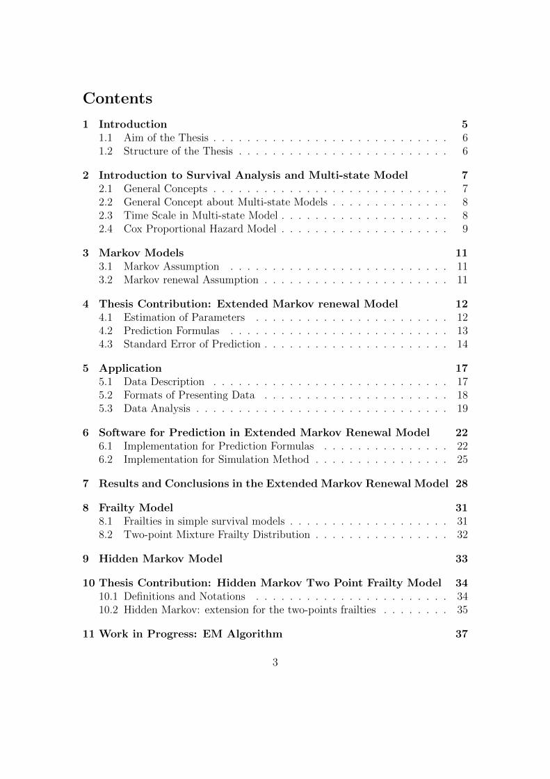
1 Introduction 51.1 Aim of the Thesis . . . . . . . . . . . . . . . . . . . . . . . . . . . . 61.2 Structure of the Thesis . . . . . . . . . . . . . . . . . . . . . . . . . 6

2 Introduction to Survival Analysis and Multi-state Model 72.1 General Concepts . . . . . . . . . . . . . . . . . . . . . . . . . . . . 72.2 General Concept about Multi-state Models . . . . . . . . . . . . . . 82.3 Time Scale in Multi-state Model . . . . . . . . . . . . . . . . . . . . 82.4 Cox Proportional Hazard Model . . . . . . . . . . . . . . . . . . . . 9

3 Markov Models 113.1 Markov Assumption . . . . . . . . . . . . . . . . . . . . . . . . . . 113.2 Markov renewal Assumption . . . . . . . . . . . . . . . . . . . . . . 11

4 Thesis Contribution: Extended Markov renewal Model 124.1 Estimation of Parameters . . . . . . . . . . . . . . . . . . . . . . . 124.2 Prediction Formulas . . . . . . . . . . . . . . . . . . . . . . . . . . 134.3 Standard Error of Prediction . . . . . . . . . . . . . . . . . . . . . . 14

5 Application 175.1 Data Description . . . . . . . . . . . . . . . . . . . . . . . . . . . . 175.2 Formats of Presenting Data . . . . . . . . . . . . . . . . . . . . . . 185.3 Data Analysis . . . . . . . . . . . . . . . . . . . . . . . . . . . . . . 19

6 Software for Prediction in Extended Markov Renewal Model 226.1 Implementation for Prediction Formulas . . . . . . . . . . . . . . . 226.2 Implementation for Simulation Method . . . . . . . . . . . . . . . . 25

7 Results and Conclusions in the Extended Markov Renewal Model 28

8 Frailty Model 318.1 Frailties in simple survival models . . . . . . . . . . . . . . . . . . . 318.2 Two-point Mixture Frailty Distribution . . . . . . . . . . . . . . . . 32

9 Hidden Markov Model 33

10 Thesis Contribution: Hidden Markov Two Point Frailty Model 3410.1 Definitions and Notations . . . . . . . . . . . . . . . . . . . . . . . 3410.2 Hidden Markov: extension for the two-points frailties . . . . . . . . 35

11 Work in Progress: EM Algorithm 37

3

12 Discussion 40

Appendix A Functions Defined for the Analysis 45

Appendix B Codes for the Analysis 51

4

1 Introduction

Multi-state models are widely used for describing the longitudinal progressionof subjects between a finite number of states, who are exposed to several time-dependent stochastic events. Occurrence of an event, resulting in change of state,is called transition. In medical application, multi-state models are useful tools formodeling the disease process of patients when intermediate events of interest canoccur during the follow-up time [1].This class of models can allow much flexibility when interests are in multiple sur-vival outcomes. In a breast cancer trial, for instance, intermediate events likerecurrence of tumor in the vicinity of the primary tumor (local recurrence), or atdistant locations (distant metastasis) occur after surgery of the primary tumor.Figure 1 shows an example multi-state model for such trial. A patient can expe-rience relapse-free survival, local recurrence, distant metastasis or both after thesurgery, and may eventually end up in the absorbing state death. Clinicians mightbe interested in evaluating influence of several treatments on both overall survivaland occurrence of the intermediate events. In these situations, multi-state modelcan be used to model patient’s history, and evaluate the influence of prognosticfactors on possible transitions between the states. It is also valuable to predictprobabilities of visiting a certain state within a given time for a patient with spe-cific clinical prognosis by employing such models [2].

Surgery

Local recurrence

Distantmetastasis

Local recurrenceand Distantmetastasis

Death

Figure 1: An example multi-state model for breast cancer trail

5

1.1 Aim of the Thesis

Often when employing a multi-state model, the Markov assumption is adoptedto simplify the inference process. The Markov property states that the futuredepends on the history only through the present. For a multi-state model thismeans that, given the present state and the event history of a patient, the nextstate to be visited and the time at which this will occur will only depend on thepresent state. However, this assumption might fail to hold in some applications,leading to inconsistent estimates.The goal of this thesis is to address the violation of Markov assumption in multi-state model by proposing two new methods.The first method is an extension of Markov renewal model. Here an extra covariateto account for transition time to intermediate event is introduced. Formulas aredeveloped to obtain the prediction for transition probabilities in an illness-deathextended Markov renewal model. General functions are written in R to make themethod developed in this thesis applicable to data set that can be described by anillness-death model.The second approach combines hidden Markov model and the two-point mixturefrailties. This model can deal with the association between transition times aswell as the violation of Cox proportional hazard assumption. An EM algorithm isproposed to implement this method.

1.2 Structure of the Thesis

Basic concepts of survival analysis and multi-state model are described in Chapter2. In Chapter 3, a brief introduction to Markov and Markov renewal modelsis given. Our first proposed method extended the Markov renewal model andit is described in Chapter 4 along with specific formulas for prediction and thesimulation algorithm. In Chapter 5 the model is applied to a breast cancer dataset. Details concerning the softwares written to implement the proposed methodare given in Chapter 6. The results and conclusions concerning the application ofthe extended Markov renewal model to the breast cancer data set are outlined inChapter 7.The second part of this thesis concerns frailty and hidden Markov model. A shortintroduction to frailty model and hidden Markov model is given in Chapter 8 and9 respectively. To deal with possible association between transitions a hiddenMarkov two-point frailty model is proposed in Chapter 10 and an EM algorithmis outlined in Chapter 11. All R code written for this thesis can be found in theappendices.

6

2 Introduction to Survival Analysis and Multi-

state Model

In this section, a summary of the basic mathematic theory underlying survivalanalysis and multi-state will be presented.

2.1 General Concepts

Survival analysis studies the distribution time from an initiating state (like birth,start of treatment) to some terminal event (like death, relapse). Let T be therandom variable representing the interval length from the starting point to theoccurrence of the event of interest. The survival function S(t) represents theprobability that a population survives at least until time t and it is defined as

S(t) = P (T > t).

Let F (t) be the cumulative distribution function of T , i.e. F (t) = P (T ≤ t). Thesurvival function is the complement of the cumulative distribution S(t) = 1−F (t).The survival can be also expressed as

S(t) = P (T > t) =

∫ ∞t

f(v)dv.

Hazard rate function h(t) expresses the rate at which an individual who is event-free at time t will experience the event of interest in the next instant. It is definedas

h(t) = lim∆t→0

P (t ≤ T ≤ t+ ∆t|T > t)

∆t.

The cumulative hazard function is given by

H(t) =

∫ t

0

h(v)dv,

which is a measure of risk of the occurrence of event.If the random variable T is continuous the relation between survival and cumulativehazard is as follow

S(t) = exp(−H(t)) = exp(−∫ t

0

h(v)dv).

7

2.2 General Concept about Multi-state Models

Denote by S = {1, ..., r} the states in the multi-state model; let X(t) and Ht−be a stochastic process taking a value in S at time t and the history observationsof the disease process over time interval [0, t) respectively. The hazard function,or transition intensity, which expresses the instantaneous risk of a transition fromstate g to state h at time t is defined as

αgh(t) = lim∆t→0

P (X(t+ ∆t) = h|X(t) = g,Ht−)

∆t.

The cumulative transition hazard is as follow

Agh(t) =

∫ t

0

αgh(u)du.

If a direct transition between state g and state h cannot occur, Agh(t) ≡ 0. Theintensity matrix A(t) can be constructed into a r × r-matrix, with non-diagonalelements Agh(t) ∀g 6= h and diagonal elements Agg(t) = −

∑g 6=h Agh(t).

The transition probability Pgh(s, u) is often the prime quantity of interest. It isdefined as

Pgh(s, u) = P (X(u) = h|X(s) = g,Hs−), (1)

which denote transition probability of going from state g to state h in time interval(s, t] given the patient’s history.

2.3 Time Scale in Multi-state Model

For the definition of time t in the hazard functions α(t) defined in Section 2.2, twodistinct approaches are often used in multi-state models, which are denoted hereby the ‘clock forward’ or ‘clock reset’ approach.‘Clock forward’: in this approach, time t refers to the time since patient enters theinitial state. That means the clock starts with 0 at entrance of the initial stateand then keeps moving forward.‘Clock reset’: in this approach, time t refers to the time since patient enters thecurrent state. That means the clock is set back to 0 each time the patient entersa new state.The difference between the two approaches is illustrated by a cancer patient’s dis-ease progress (Figure 2). The upper graph shows the calendar date of surgery andsubsequent events. The patient is censored for death due to the end of follow-up.The lower graph compares the two different time scales. In the ‘clock forward’ ap-proach, time is measured by years from the date of surgery, whereas in the ‘clockreset’ approach, time is measured by time intervals between occurrence of events.

8

surgery

0clock forward:

clock reset:

LR

2.252.25

DM

6.754.5

FUP

11.364.61

calendar time scale

date of surgery

1/1/1994

date of LR

1/4/1996

date of DM

1/10/2000

end of follow-up

13/05/2005

Figure 2: Illustration of the ‘clock forward’ and ‘clock reset’ approach.(LR, DM and FUP stand for local recurrence, distant metastasis and follow-up, respectively.)

2.4 Cox Proportional Hazard Model

Cox proportional hazard model, often abbreviated to Cox model or proportionalhazard model, is widely used to quantify the covariate effects on survival [3]. Underthe proportional hazard assumption the effect of a unit increase in a covariate ismultiplicable with respect to hazard rate. This model can be employed in multi-state model to evaluate effects of prognostic factors on different transitions. Fora patient with covariate vector Z, the transition-specific hazard rate transitiong → h is given by

αgh(t) = αgh,0(t) exp(β>ghZ)

where αgh,0(t) is the baseline hazard of transition g → h, and βgh is the vector ofregression coefficients.The model can be also written as

αgh(t) = αgh,0(t) exp(β>Zgh)

where Zgh is a vectors of covariates specific to transition g → h , defined for theindividual based on her covariates Z [5]. Denote by Zgh,i the transition-specific

covariates of patient i for transition g → h. Estimates β can be obtained togetherby maximizing the generalized Cox partial likelihood

L(β) =∏

transitiong→h

n∏i=1

i:dgh,i=1

exp(β>Zgh,i)∑j∈Rg(tgh,i)

exp(β>Zgh,j)

9

where tgh,i is the failure or censoring time of individual i for transition g → h,dgh,i = 1 if individual i has an event for transition g → h, 0 otherwise, andRg(tgh,i) is the risk set of individuals who are in state g at time t (t being here thetime since entry in state g). The Nelson-Aalen estimate of the cumulative baselinehazard of transition g → h is given as follow

Agh,0(t) =n∑

i=1tgh,i≤t

dgh,i∑j∈Rg(tgh,i)

exp(β>Zgh,j)

10

3 Markov Models

3.1 Markov Assumption

In applications of multi-state models, Markov assumption is often adopted. TheMarkov property assumes that the future evolution of process only depends on thecurrent state. Under the Markov assumption, the transition probability defined in(1) satisfies

Pgh(s, u) = P (X(u) = g|X(s) = h) (2)

Markov property drastically simplifies the inference of likelihood, and under suchassumption the estimation of transition probabilities can be expressed as a functionof transition intensities in the form of product integral [6]:

P (s, u) =∏(s,u]

(I + dA(t)).

Usually, “clock-forward” approach is used for Markov model, which means that thetime scale is the calendar time since the origin of the process.

3.2 Markov renewal Assumption

If the transition intensities depend on the history not only through the currentstate but also on the sojourn time in the current state, the multi-state modelbecomes a Markov renewal model. It is also defined as semi-Markov model [7-11]. To define the Markov renewal property, we shall use the definitions and theformalism of Dabrowska et al. [10-11].Let 0 = T0 < T1 < ... < Tm be consecutive times of entrance into the statesS0, S1, ..., Sm ∈ {1, ..., r}, then (S, T ) = (S`, T`)`>0 forms a Markov renewal processif the sequence of states visited S = (S` : ` > 0) is a Markov chain and the sojourntimes Jm+1 = Tm+1 − Tm satisfy:

P{Sm+1 = j, Jm+1 ≤ τ|S0, T0, ..., Sm, Tm} = P{Sm+1 = j, Jm+1 ≤ τ|Sm}.

For Markov renewal models, “clock-reset” approach is commonly used due tothe renewal nature of the process.

11

4 Thesis Contribution: Extended Markov renewal

Model

In some applications both Markov and Markov renewal assumption could fail tohold due to the presence of association between transition times. In this section,Markov renewal assumption will be further relaxed to allow the transition inten-sities to depend on the sojourn time of earlier states. Since it is an extension ofMarkov renewal model, this model will be defined as extended Markov renewalModel. Similar to Markov renewal model, the “clock-reset” approach will be usedfor the definition of time t in the hazard function α(t).

4.1 Estimation of Parameters

Similar to the prognostic covariates, effects of sojourn time in earlier states canbe estimated by employing Cox proportional hazard model. For a patient withassociated prognostic covariate vector Z and time vector J , the transition hazardαgh(t) for transition g → h is given by

αgh(t) = αgh,0(t) exp(β>Zgh + γ>Jgh)

where αgh,0(t) is the baseline hazard of transition g → h, β and γ are vectorsof regression coefficient respectively corresponding to Zgh and Jgh; and Jgh is thevector of sojourn times specific to transition g → h. Note that Jgh only containssojourn time of states no later than the gth state.Similarly to the procedure introduced in Section 1.4, estimates β, γ and the cu-mulative baseline hazards Agh,0(t) can be obtained together by maximizing thegeneralized Cox partial likelihood

L(β, γ) =∏

transitiong→h

n∏i=1

i:dgh,i=1

exp(β>Zgh,i + γ>Jgh,i)∑j∈Rg(tgh,i)

exp(β>Zgh,j + γ>Jgh,j)

where tgh,i is the failure or censoring time of individual i for transition g → h,dgh,i = 1 if individual i has an event for transition g → h, 0 otherwise, andRg(tgh,i) is the risk set of state g at time t, i.e. the set of individuals who are instate g at time t (t being here the time since entry in state g). The estimate ofthe cumulative baseline hazard of transition g → h is the Nelson-Aalen estimate:

Agh,0(t) =n∑

i=1tgh,i≤t

dgh,i∑j∈Rg(tgh,i)

exp(β>Zgh,j + γ>Jgh,j).

12

Surgery (1)

Recurrence (2)

Death (3)

Figure 3: A Illness-Death Model for the Breast Cancer Trial

4.2 Prediction Formulas

The general problem is to estimate the conditional probabilities of some clinicalfuture events, given the patient’s history and a set of values for prognostic factorsZ. The estimate of these probabilities are based on the results obtained from theCox model on the transition hazard between states.It is not possible to write down explicitly the transition probability for a generalnon-Markov multi-state model. However in case of an illness death model whereonly three states are present (see Figure 3), it is possible to derive the predictionprobability.In this illness-death model, local recurrence, distant metastasis and the joint ofboth are taken together as one intermediate event, in short termed “Recurrence”.After surgery, a patient may die before or after experiencing tumor recurrence.The three possible states “Surgery”, “Recurrence” and “Death” are respectivelynumbered by 1, 2 and 3. In this model there are three possible paths that a patientmay follow after surgery: from surgery to recurrence (1→ 2); direct transition fromsurgery to death (1→ 3); from surgery to recurrence to death (1→ 2→ 3).

The probabilities can be expressed in terms of the hazard rate for each transi-tion.For a patient without recurrence to s years post-surgery, the probability that thepatient remains in state 1 in the time interval (s, t] is given by

P11(s, t|Z) = exp(−∫ t

s

(α12(u|Z) + α13(u|Z))du), (3)

where α12(u|Z) and α13(u|Z) are the transition hazards respectively correspondingto transition 1 → 2 and 1 → 3 given the patient’s covariates, Z is the vector ofcovariates.The conditional probability of being in state 2 at time t given an individual is instate 1 at time s is as follow

P12(s, t|Z) =

∫ t

s

α12(u|Z)P11(s, u−|Z)P u22(u, t|Z)du. (4)

13

The probability of remaining in state 2 in the time interval (s,t] can be com-puted as

P r22(s, t|Z) = exp(−

∫ t

s

α23,r(u− r|Z)du), (5)

where r is the entrance time of state 2 (r ≤ s) and

α23,r(u|Z) = α23,0(u) exp(βTZ + γ2r).

The probability of death is given by

P r23(s, t|Z) = 1− P r

22(s, t|Z). (6)

There are two possible paths going from state 1 to state 3. To distinguish them,we denote the probability of direct transition from surgery to death as P 1

13(s, t),

P 113(s, t|Z) =

∫ t

s

α13(u|Z)P11(s, u−|Z)du. (7)

The probability that tumor recurrence and later on death occur during time inter-val (s, t] is given by

P 213(s, t|Z) =

∫ t

s

α12(u|Z)P11(s, u−|Z)P u23(u, t|Z)du. (8)

Note that for the transition probability P u23(u, t)du is as in (6).

4.3 Standard Error of Prediction

In Fiocco et al. [12], a simulation-based approach is proposed to obtain confidenceintervals (CIs) for the estimated prediction probabilities. This method can gen-erate paths through the multi-state model, and build bootstrap data sets that inturn can be used to obtained CIs for the estimate of interest.In this section, a brief description how to generate path through a multi-statemodel based on given cumulative hazard functions specified for each of the directtransitions and how to estimate the standard errors of predicted probabilities byapplying bootstrap resampling method will be given on. The basic idea is is in-spired by Dabrowsa [11] where a multi-states model is seen as made of severalcompeting risk blocks linked together and to simulate transition times and statesfor each such block in the multi-state model.

Generating simulated path for a specific patient can be done as follow

14

Algorithm 4.3.1Repeat, for m = 1, ...,M ,1. Let J be the set of states that can be reached from state g. If J = ∅,stop. Otherwise, let, for h ∈J , Agh(t) be the cumulative hazard function fortransition g → h.2. Compute Ag(t) =

∑h∈J Agh(t).

3. Sample t∗(> Tg) from Ag(t) −Ag(tg). If Ag(∞) is finite, t∗ = ∞ may besampled with positive probability.4. Stop if t∗ =∞. Otherwise, select state h as the next state with probabilitydAgh(t

∗)/dAg(t∗).

5. Set g = h and Tg = t∗

6. Repeat 1-5 until no further state can be reached or t∗ = ∞ is sampled.Save the simulated path as Pm

This process can be also used to estimate prediction probabilities for an ex-tended Markov renewal multi-state model, but it is less efficient than computationsbased on (3-8), since the simulation number M need to be large enough to obtainprecise estimation. Another important use of this process is to obtained CIs ofprediction possibilities, by combining with bootstrap resampling.Let B be the number of bootstrap samples.The algorithm is described as follow

Algorithm 4.3.2Repeat, for b = 1, ..., B,1. Create a resampled data set X∗b with replacement.

2. From X∗b , estimate the regression coefficients β∗b , γ∗b , and the baseline haz-

ard functions A∗gh,0(t) for all g → h transitions in the model.

3. Calculate the patient specific hazard function A∗gh(t)=A∗gh,0(t) exp(β∗bZgh+γ∗bJgh).

4. SimulateM paths through the multi-state model from A∗gh based on Algo-

rithm 4.3.1, and estimate the prediction probabilities P ∗M. Set P ∗M,b equal to

P ∗M.

Once all probabilities P ∗M,b, b = 1, ..., B have been simulated, the 95% con-

fidence interval for P ∗M can be obtained by compute 2.5%-quantile and 97.5%-

quantile of the vector {P ∗M,b|b = 1, ..., B}. Confidence interval instead of standarderror is used because probabilities are bounded by [0,1].It is important to note that the use ofM can be (much) smaller than M . Because

the computation of standard errors for P ∗M involves two nested sets of simulations,the creation of bootstrap data sets and the subsequent simulations within eachdata set to obtain the bootstrap prediction probability P ∗M. (See Fiocco et al. [12]

15

for all details).

An alternative to Algorithm 4.3.2 is to apply (3-8) instead of simulating paths

to estimate prediction probabilities. After probabilities P ∗b are estimated for allresample data set X∗1 , ..., X

∗b , 95% CIs can be obtained in the same way as described

above.

16

5 Application

In this section, the extended Markov renewal model will be employed to analyzebreast cancer data from EORTC-trail. All analysis have been performed in R.

Table 1: Prognostic factors for all patients (n = 2795)

Prognostic factor n (%)Tumor size

≤2 cm 823 (30)2-5 cm 1759 (64)> 5 cm 166 (6)Missing 47

Nodal statusNegative 1467 (53)Positive 1327 (47)Missing 1

Type of surgeryMastectomy RT 658 (24)Mastectomy, no RT 577 (21)Breast conserving 1560 (56)Missing 16

Perioperative chemotherapyNo 1395 (50)Yes 1398( 50)Missing 2

Adjuvant chemotherapyNo 2227 (82)Yes 502 (18)Missing 66

Age(years)≤50 1118 (40)> 50 1677 (60)

( “RT” stands for radiation treatment)

5.1 Data Description

The dataset originates from a clinical trail in breast cancer, conducted by Euro-pean Organization for Research and Treatment of Cancer (EORTC-trail 10854)

17

Table 2: Number of patients to enter and visit the states.

State No. to enter No. to visit1 2 3 no events

1 2687 - 1060(39.5%) 84(3.1%) 1543(57.4%)2 1060 - - 645(60.8%) 415(39.2%)3 84 - - - -

[13]. The aim of the trial was to study whether a short intensive course of pre-operative polychemotherapy yields better therapeutic result than surgery alone.The trial include women with early breast cancer, who underwent either radicalmastectomy or breast conserving therapy before being randomized. The Trial con-sisted of 2795 patients, randomized to either chemotherapy or no chemotherapy.Details of the trail [13] and long-term results [14] can be found in [13-14]. Medianfollow-up was 10.8 years. The most important prognostic factors are shown inTable 1. Most of these factors contain a small number of missing values. Ouranalysis will be based on the patients with full information (n=2687, 96.1%).The illness-death model described in Section 2.2.2 (Figure 3) was applied to thisdata set. The number of patients to enter and to visit each state are shown inTable 2.

5.2 Formats of Presenting Data

As a preliminary, two ways of representing the same data will be introduced in thissection. The first of these is the one-row-per-subject format (the ‘wide’ format).Here below an example for the first three patients from the data set under studyis shown:

id time rec status rec time surv status surv periop1 -189 2.007 1.000 3.978 1 no periop chemo2 -188 13.380 0.000 13.380 0 periop chemo3 -187 1.276 1.000 3.433 1 no periop chemo

The variables time_rec and time_surf are used to indicate occurrence (or censor-ing) time of tumor recurrence and death respectively. The variables status_rec

and status _surv are used to indicate whether the occurrence of events has been

18

observed (1 observed event and 0 for censored). An alternative way of representingthe same data is in the so-defined ‘long’ format. This format allows most flexibilityfor multi-state modeling. The same data in the ‘long’ format is as follow

id from to trans Tstart Tstop time status periop.1 periop.2 periop.31 -189 1 2 1 0.000 2.007 2.007 1 0 0 02 -189 1 3 2 0.000 2.007 2.007 0 0 0 03 -189 2 3 3 2.007 3.978 1.971 1 0 0 04 -188 1 2 1 0.000 13.380 13.380 0 1 0 05 -188 1 3 2 0.000 13.380 13.380 0 0 1 06 -187 1 2 1 0.000 1.276 1.276 1 0 0 07 -187 1 3 2 0.000 1.276 1.276 0 0 0 08 -187 2 3 3 1.276 3.433 2.157 1 0 0 0

For each individual a row is added for each possible transition at each state. i.e. Forpatient 189, who entered state 2 at t = 2.007, two transitions can occur from state1: 1→ 2 and 1→ 3; it is possible to move only to state 3 from state 2: 2→ 3. Forpatient 188, who never entered state 2 during the follow-up, only two transitionsfrom state 1 are possible. There are three rows corresponding to patient 189 butonly two rows to patient 188. The variable trans was added with a unique valueto label all possible transitions transitions (1 for transition 1→ 2, 2 for transition1→ 3, and 3 for transition 2→ 3). The variables from and to are used to indicatethe starting state and ending state for each transition respectively. The variablesTstart and Tstop indicate the entering time and leaving time for each transition.The variable time is the sojourn time spent in each state, and status is usedto indicate whether the event was observed or censored. Extra dummy variables(periop.1,periop.2,periop.3) are transition-specific covariate (see Section 2.4).They have value 0 except for the patient’s condition for the transition that theycorrespond to. For instance, patients who did not receive perioperative chemother-apy are treated as reference group and dummies are coded as 0 for this treatmentgroup. For patient 188 who received perioperative chemotherapy, preriop.1= 1for transition 1 but 0 for the others, preriop.2= 1 for transition 2 but 0 for others.

5.3 Data Analysis

Cox regression model was fitted to the data by including all prognostic covariatesand the sojourn time covariate. The results are summarized in Table 3.

Positive nodal status significantly increases transition rates for all transitions(0.443(0.075) for transition 1→ 2, 0.801(0.253) for transition 1→ 3, 0.750(0.095)for transition 2→ 3). Large tumor size has similar effects, but it is not significant

19

Table

3:

Para

met

eres

tim

ates

and

stan

dar

der

rors

for

all

cova

riat

esan

dal

ltr

ansi

tion

s..

1→

21→

32→

3C

oef

(SE

)P

-valu

eC

oef

(SE

)P

-valu

eC

oef

(SE

)P

-valu

eT

um

or≤

2cm

2-5

cm0.2

96(0

.075)

<0.0

001

-0.0

35(0

.260)

0.8

90.1

22(0

.106)

0.2

5>

5cm

0.77

1(0

.132)

<0.0

001

0.7

33(0

.420)

0.0

81

0.3

05(0

.167)

0.0

67

Nodal

Neg

ativ

eP

osit

ive

0.44

3(0

.075)

<0.0

001

0.8

01(0

.253)

0.0

02

0.7

50(0

.095)

<0.0

001

Su

rger

yM

ast,

RT

Mas

t,n

oR

T0.0

06(0

.097)

0.9

51.0

21(0

.312)

0.0

01

0.1

59(0

.118)

0.1

8B

CT

-0.0

12(0

.081)

0.8

80.0

89(0

.312)

0.7

7-0

.123(0

.100)

0.2

2P

erio

-p

erat

ive

No

Yes

-0.1

45(0

.0615)

0.0

19

-0.1

31(0

.219)

0.5

50.0

45(0

.080)

0.5

5A

dju

vant

chem

oth

erap

yN

oY

es-0

.295(0

.103)

0.0

04

0.4

36(0

.397)

0.2

7-0

.033(0

.120)

0.7

9A

ge(y

ears

)≤

50>

50-0

.159(0

.076)

0.0

37

0.6

17(0

.305)

0.0

43

0.0

83(0

.094)

0.3

8T

ime

ofre

curr

ence

-0.1

53(0

.0186)

<0.0

001

20

for transitions to death. Young age is a well know risk factor for recurrence and thiscan be seen from Table 3 (-0.159(0.076)), as well as the reverse effect for transitionto death (0.617(0.305)). Perioperative chemotherapy and Adjuvant chemotherapysignificantly decrease the transition rate for transition from surgery to tumor re-currence. Mastectomy without radiation treatment increase the transition ratefrom surgery to death comparing to Mastectomy with radiation treatment. Thesignificant estimated time coefficient (-0.153(0.0186)) indicates violation of Markovproperty: the time at which tumor recurrence occurred has a significant effect ontransition from recurrence to death. Early recurrence increases the risk of death.

The estimated baseline survival curves for all three transitions (values of co-variates are as follow tumor size <2 cm, negative axillary nodes, type of surgery= mastectomy + radiotherapy, no perioperative and no adjuvant chemotherapy,age ≤ 50 years, and time of recurrence =0) are plotted in Figure 4.

Figure 4: Baseline survival curves for all transitions

21

6 Software for Prediction in Extended Markov

Renewal Model

6.1 Implementation for Prediction Formulas

To implement prediction for the extended Markov renewal model in R, new func-tions getlevel(), dataprep(),predict(), plot.predict() and prob.predict()

were written for estimating and plotting prediction results. In this section, briefintroduction and examples will be given. The detailed codes can be found in Ap-pendix A.Suppose we are interested on the future disease development of a patient A whohas the following prognostic covariates: tumor size >5 cm, positive lymph nodestatus, mastectomy plus radiotherapy, no perioperative chemotherapy, no adjuvantchemotherapy, age≤ 50 years. The input for the patient A’s data in R (which isusually in ‘wide’ format) is as following

> print(y)

periop surgery tusi nodal adjchem age50

1 no periop chemo mastectomy with RT >5 cm node positive no adj chemo <=50

The first step is to prepare the data into the long format with transition-specificcovariates (see Section 1.2). The function dataprep() can rearrange the data fromwide format into ‘long’ format, by specifying the data to be rearranged, names ofthe covariates, the fitted multi-state model, and the levels of categorical variables.For categorical variables the function getlevel() will give levels for all variablesof interest at once. An example of how the two functions work is shown below.Use the function getlevel() to obtain the variable levels.

> load("bc.long")

> covs<-c("periop", "surgery", "tusi", "nodal", "age50", "adjchem")

> (lvls<-getlevel(covs,bc.long))

$periop

[1] "no periop chemo" "periop chemo"

$surgery

[1] "mastectomy with RT" "mastectomy without RT" "breast conserving"

$tusi

[1] "<2 cm" "2-5 cm" ">5 cm"

22

$nodal

[1] "node negative" "node positive"

$age50

[1] "<=50" ">50"

$adjchem

[1] "no adj chemo" "adj chemo"

The function dataprep() transforms the new data into the wide format withtransition-specific covariates.

> fit<-coxph(Surv(time,status)~.-trans+strata(trans), bc.long[,-c(1:3,6,9:15)])

> print(newdata<-dataprep(y,covs,fit,lvls))

trans Tstart adjchem.1 adjchem.2 adjchem.3 age50.1 age50.2 age50.3 nodal.1

1 1 0 0 0 0 0 0 0 1

2 2 0 0 0 0 0 0 0 0

3 3 0 0 0 0 0 0 0 0

nodal.2 nodal.3 periop.1 periop.2 periop.3 surgery1.1 surgery1.2 surgery1.3

1 0 0 0 0 0 0 0 0

2 1 0 0 0 0 0 0 0

3 0 1 0 0 0 0 0 0

surgery2.1 surgery2.2 surgery2.3 tusi1.1 tusi1.2 tusi1.3 tusi2.1 tusi2.2

1 0 0 0 0 0 0 1 0

2 0 0 0 0 0 0 0 1

3 0 0 0 0 0 0 0 0

tusi2.3

1 0

2 0

3 1

The function dataprep() can also be used to prepare data of a single patientfor the function msfit() in the {mstate} package [16], which is used to computesubject-specific or overall cumulative transition hazards for each of the possibletransitions in Markov multi-state model.

After the data is reshaped into wide format the function predict(), which isbased on the formulas given in Section 4.2, can be used to predict transition prob-abilities given the patient’s history at time point (t). If a patient A is alive withouttumor recurrence at 2 years post-surgery, the predicted transition probabilities canbe obtained by the following codes:

23

> results<-predict(fit,newdata,t=2,bt="Tstart")

The argument bt=“Tstart” is to specify name of the estimated coefficient corre-sponding to time variable.The returned object results contains two objects: a data frame called “probs”which contains time points and the corresponding estimated transition probabili-ties and a list called “hazards” which contains the estimated cumulative hazards.Examples of the estimated transition probabilities are shown below

time P11 P122 P123 P13

[1,] 2.726899 0.7950662 0.1646767 0.03061893 0.009362081

[2,] 2.973306 0.7423555 0.1889760 0.05474760 0.013582195

[3,] 3.370294 0.6612630 0.2207091 0.10165261 0.015937783

[4,] 4.284736 0.5261654 0.2261588 0.22322631 0.023834284

[5,] 6.409309 0.3508181 0.1709543 0.44620436 0.031168458

P11, P122, P123, P13 respectively stand for probability of disease-free survival,probability of survival with tumor recurrence, probability of death after tumorrecurrence and probability of death without tumor recurrence.

For a patient who has already experienced recurrence, the occurrence time ofrecurrence needs to be specified for the Tstart variable. The returned list ofprediction probabilities only contains two columns: P22 and P23, which are re-spectively the probability of survival with recurrence and the probability of death.Function predict() can be used to predict transition probabilities for Markovrenewal model, by specifying the time coefficient bt= NULL.

The function plot.predict() produces survival curves by using the output ofpredict. An example is shown in Figure 5. The plot shows the predicted transi-tion probabilities for patient A given that no events have occurred during the firsttwo years after surgery. The probabilities are stacked; the height of each band isthe probability of the path. The paths are ordered from top to bottom accordingto increasing disease severity.

The function prob.predict() produces estimated transition intensities at cer-tain time point t by using output from the function predict(). Suppose thatclinicians are interested in predicting the specific status for patient A at t = 6years post-surgery. The transition intensities can be obtained as:

> prob.predict(t=6,results$probs)

P1 P2 P3

0.3807090 0.1763831 0.4420988

24

Figure 5: Prediction results: plot by plot.predict()

where P1, P2, P3 respectively stand for probability of disease-free survival, proba-bility of survival with recurrence and probability of death, the subscript numbersindicating the state occupied at time t.

6.2 Implementation for Simulation Method

In [12] the functions mssample() and msboot() have been used to compute pre-diction probabilities and their confidence intervals and standard errors of the re-gression coefficients in multi-state reduced rank models. The same procedure willbe employed to estimate the confidence intervals for prediction probabilities in ourextended Markov renewal model. A brief description of the two functions will begiven in this section. All details concerning the R code can be found in Appendix B.

The function mssample() implements Algorithm 4.3.1 to generate a specified

25

number of paths through the multi-state model and computes probabilities ofstates and paths given the starting state and time. As mentioned in Section 4.3,mssample() can also be used to obtain prediction of transition probabilities but itis less efficient than predict(). Figure 6 shows the prediction probabilities by re-spectively employing the two methods for a patient B who just underwent surgeryand who has the same prognostic covariates as patient A. As expected, the predic-tion results are very close when the simulation number M is large. Compared tosimulations by using function mssample, predict() can produce smoother curvesand provide trajectory probabilities instead of transition intensities.

Figure 6: Prediction probabilities by implementing formula (left) and simulation (right)

The function msboot() samples randomly with replacement subjects from theoriginal data set and can be used to estimate any vector-valued statistic in amulti-state model. It can be combined together with mssample() to implementthe Algorithm 4.3.2. Here below it is shown how to obtain prediction probabilitiesand confident interval for patient B (tumor size >5 cm, positive lymph node sta-tus, mastectomy plus radiotherapy, no perioperative chemotherapy, no adjuvantchemotherapy, age≤ 50 years) at t = 6 years post-surgery by using the functionspredict(), mssample() , and msboot():

> tmat <- trans.illdeath()#specify the transition matrix

26

> M=100# simulation number

> tvec=6 #time point

> history<-list(state=1,time=0,tstates=c(0,0,0)) #specify the patient's history

> theta<-function(data){

+ dat<-data[,-c(1:3,6,9:15)]

+ fit<-coxph(Surv(time,status)~.-trans+strata(trans), dat)

+ Haz<-haz(fit,newdata)

+ bt<-summary(fit)$coef[,1]["Tstart"]

+ beta.state<-matrix(0,3,3)

+ beta.state[1,2]<-bt

+ res<-mssample(Haz,trans=tmat,clock="reset",

+ history=history,beta.state=beta.state,tvec=tvec,M=M)

+ c(as.matrix(res[,-1]))

+ }

> res<-msboot(theta,bc.long,B=500,id="id") #generate bootstrap samples

> predB<-predict(fit,newdata,t=0,bt="Tstart")

> estimate<-prob.predict(t=6,predB$probs)

> LCI<-apply(res,1,function(x)quantile(x,probs=0.025))

> UCI<-apply(res,1,function(x)quantile(x,probs=0.975))

> print(CI<-cbind(LCI,estimate,UCI),digits=2)

LCI estimate UCI

P1 0.08 0.24 0.43

P2 0.04 0.12 0.21

P3 0.44 0.64 0.86

27

7 Results and Conclusions in the Extended Markov

Renewal Model

Three fictitious patients are used to show predicted probabilities: patient A, B andC with a common set of prognostic covariate values (tumor size >5 cm, positivelymph node status, mastectomy plus radiotherapy, no perioperative chemother-apy, no adjuvant chemotherapy, age≤ 50 years). For each patient, both extendedMarkov renewal model and Markov renewal model were employed to predict futuretrajectory probabilities.Figure 7a and 7b show the predicted trajectory probabilities for patient A giventhat no events have occurred during the first two years after surgery respectivelyfor extended Markov renewal model and Markov renewal model. Compared tothe extended Markov renewal model, Markov renewal model yields to more pes-simist prediction results for disease-free survival and survival with tumor recur-rence. Markov renewal model ignores the association between time at which re-currence occurs and the transition rate from recurrence to death. As mentionedin Section 3.3, early recurrence increases the risk of death. Therefore patients whoexperience recurrence at later time have lower transition rate to death.Figures 7c and 7d show the predicted trajectory probabilities for patient B who justunderwent surgery respectively for extended Markov renewal model and Markovrenewal model. Similarly to prediction results for patient A above, Markov re-newal model shows more pessimist estimation for survival with and without re-currence comparing to the extended Markov renewal model. Figure 8 shows thepredicted state probabilities with 95% confidence intervals by employing the ex-tended Markov renewal model. The probability of being alive with recurrenceinitially increases but later on decreases as time t increases. The transition proba-bility from surgery to recurrence initially increases and later on decreases, whereasthe transition probability from recurrence to death increase rapidly as time t in-creases.Figures 7e and 7f show the predicted trajectory probabilities for patient C who hasexperienced a tumor recurrence and no other event within t = 5 years after surgeryrespectively for extended Markov renewal model and Markov renewal model. Theinfluence of time r at which recurrence occurred is shown in Figure 7e, where thesurvival probabilities assuming recurrence occurred at t = 0.5, 1, 2, 4 years post-surgery are illustrated. Comparing to a patient who had recurrence half year aftersurgery a patient who had recurrence four years after surgery has higher survivalprobability.

28

(a) Prediction by extended Markov renewal model:patient A

(b) Prediction by Markov renewal model: patient A

(c) Prediction by extended Markov renewal model:patient B

(d) Prediction by Markov renewal model: patient B

(e) Prediction by extended Markov renewal model:patient C

(f) Prediction by Markov renewal model: patient C

Figure 7: Predicted probability if future trajectories for patient A, B and C

29

(a) Probability of disease-free survival (b) Probability of survival with recurrence

(c) Probability of death

Figure 8: Predicted state probability with 95% CI for patient B

30

8 Frailty Model

In the previous sections, we have introduced an extension of Markov renewal modelto deal with possible association between transitions. An alternative approach tomodel the association between transitions is throughout frailty models.

A frailty model is a model with random effects (frailty) which acts multiplica-tively on the hazard. Frailty can be interpreted as an unobserved term affectingthe transition speed of an individual or a group or cluster of individuals. Individ-uals with higher value of frailty have larger hazards and their corresponding riskof death is higher. Frailties can be used to explain effects of unobserved or unob-servable heterogeneity caused by different sources like clustered data or deviationfrom proportional hazards assumption.In multi-state model frailties can be used for different purposes. In an early pa-per of Aalen [21] frailty was applied to a time-homogeneous Markov model as ashared random term which affects the speed of the Markov process across all tran-sitions. Bhattacharya and Klein [22] used correlated gamma frailties to model theassociations between transition intensities for a non-homogeneous Markov Model.A paper of Yen et al. [23] applied frailty to account for the different underlyingpropensity for progression of premalignant lesions. Putter et al. [25] discussed therole of frailty in competing risk and in sequence of events by employing two frailtydistributions: gamma distributed frailties and two-point mixture frailties. In thisdissertation we will combine the two-point mixture frailties in [25] with hiddenMarkov model for a forward sequential process.

8.1 Frailties in simple survival models

Let T denote the survival time and suppose that conditional on a frailty Z thehazard of dying is given as follow

λ(t|Z) = Zλ(t). (9)

The latent frailty is assumed to act in a multiplicative way on the hazard; λ(t) isthe conditional hazard given Z = 1.At population level the frailty induces selection because individuals with highfrailty die first and individuals who are still alive at time t (t > 0) have thus loweraverage frailty than the population average at the start. The marginal hazard isgiven by

λ∗(t) = λ(t)E(Z|T > t). (10)

A very convenient tool for deriving properties of the population is the Laplacetransform of the frailty distribution [24] which is defined as

L(c) = E exp(−cZ). (11)

31

The marginal surivial function S∗(t) is defined as

S∗(t) = P (T > t) = E exp(−ZΛ(t)) = L(Λ(t)), (12)

where Λ(t) is the conditional cumulative hazard given Z = 1.

By the relation λ∗(t) = −d logS∗(t)/dt the marginal hazard λ∗(t) can be ex-pressed in terms of the Laplace transform as

λ∗(t) = λ(t) · −L′(λ(t))

L(λ(t)). (13)

8.2 Two-point Mixture Frailty Distribution

Many distributions can be chosen for frailty. The most commonly used frailtydistribution is the gamma distribution for its convenience in mathematical com-putation. In this dissertation we will focus on the two-point mixture frailty withdistribution P (Z = 1) = 1 − π and P (Z = θ) = π, which is less often used butalso convenient from computational and analytical perspective. For identifiabilityreasons, it is assumed that θ > 1. Its expectation is π(θ− 1) + 1, and the varianceis π(1− π)(θ − 1)2. The Laplace transform is given by

L(c) = E exp(−cZ) = (1− π)e−c + πe−θc. (14)

From (12) the marginal survival function is

S∗(t) = L(Λ(t)) = (1− π)e−Λ(t) + πe−θΛ(t) (15)

From (13) the marginal hazard rate is

λ∗(t) = λ(t) · 1− π + θπe−(θ−1)Λ(t)

1− π + πe−(θ−1)Λ(t). (16)

The fraction of alive population changes over time as a result of selection. Thepopulation fraction for patients that survive to time t P (Z = θ|T > t) is given as

P (Z = θ|T > t) =P (Z = θ, T > t)

P (T > t)=

πe−θΛ(t)

(1− π)e−Λ(t) + πe−θΛ(t). (17)

32

9 Hidden Markov Model

A hidden Markov model (HMM) is a statistical model in which the underlyingstochastic process is assumed to be Markovian but not observable (“hidden”). Theunderlying stochastic process can produce another set of observed variables, whichcould be either discrete or continuous. To define a hidden Markov model, thedefinitions and formalism in Rabiner and Juang [26] will be used.Denote by Q = {Q1, Q2, ..., QN} the hidden states at a sequence of time pointst1 < t2 < ... < tN . Let O = {O1, O2, ..., ON} be the observation sequence. Underan HMM two independence assumptions are made about the hidden and observedvariables: (i) given the kth hidden variable the (k + 1)th hidden variable is inde-pendent of all previous variables, or

P (Qk+1|Qk, Ok, ..., Q1, O1) = P (Qk+1|Qk); (18)

(ii) given the kth hidden variable the kth observation is independent of other vari-ables or

P (Ok|Qk, Qk−1, Ok−1, ..., Q1, O1) = P (Ok|Qk). (19)

Based on assumption (i) the transition probability matrix can be defined as

A = {αgh}, αgh = P (Qk+1 = h|Qk = g). (20)

Based on assumption (ii)

B = {bg(k)}, bg(k) = P (Ok|Qk = g), (21)

where bg(k) is the probability of observation Ok at time point tk in state g.The initial state distribution at time point t1 is defined as

π = {πg}, πg = P (Q1 = g). (22)

The complete set of (A,B, π) can be used to specify an HMM. In applicationof HMM, there are three key problems of interest [26]:

1. Compute the probability of observation sequence given the HMM model(A,B, π) and the observation sequence O = O1, ..., ON .

2. Find the best hidden states sequence Q1, ..., QN for a given observation se-quence O = O1, ..., ON .

3. Find the optimal model parameters (A,B, π) to maximize P (O|A,B, π).

33

10 Thesis Contribution: Hidden Markov Two

Point Frailty Model

The idea behind two-point mixture frailty model assumes that there is a latentclass of individuals who experienced the transition at a normal speed, as well asa class of individuals who experienced the transition at a higher speed. The firstclass can be referred as normal class or “class 0”, while the second class can bereferred as frail class or “class 1”. The latent class to which an individual belongscannot be observed but could influence the hazard rate and thereby be estimatedfrom the occurrence of events and corresponding sojourn times. This plays a rolesimilar to hidden states in an hidden Markov model. The difference between thetwo approaches is that in a two-point frailty model an individual belongs to onelatent class across all transitions.By extending the two-point frailty model we propose a hidden Markov two-pointmixture model which allows latent frailty of patients varies for different transitions.The new model contains two hierarchies: the first part concerns the variation offrailties across different transitions and the second part concerns the hazard andsurvival function for given frailty in each transition.In this section the hidden Markov two-point mixture model will be illustrated byapplying it to a forward sequential process in breast cancer trial (see Figure 9).

Surgery LR DM Death1 2 3

Figure 9: A multi-state model in sequence for a breast cancer trail.

10.1 Definitions and Notations

In the multi-state state model shown in Figure 9 there are three transitions: fromsurgery to local recurrence (transition 1), from local recurrence to distant metas-tasis (transition 2), from distant metastasis to death (transition 3).Let tij and δij denote time and status for individual i and transition j respectivelywith i = 1, ..., n and j = 1, 2, 3. The indicator function δij is defined as

δij =

{1, if transition j occurs for patient i

0, otherwise

It is obvious that transition 2 can be observed only after transition 1 has occurred(δi1 = 1). The same holds for transition 3 (δi1 = 1, δi2 = 1).

34

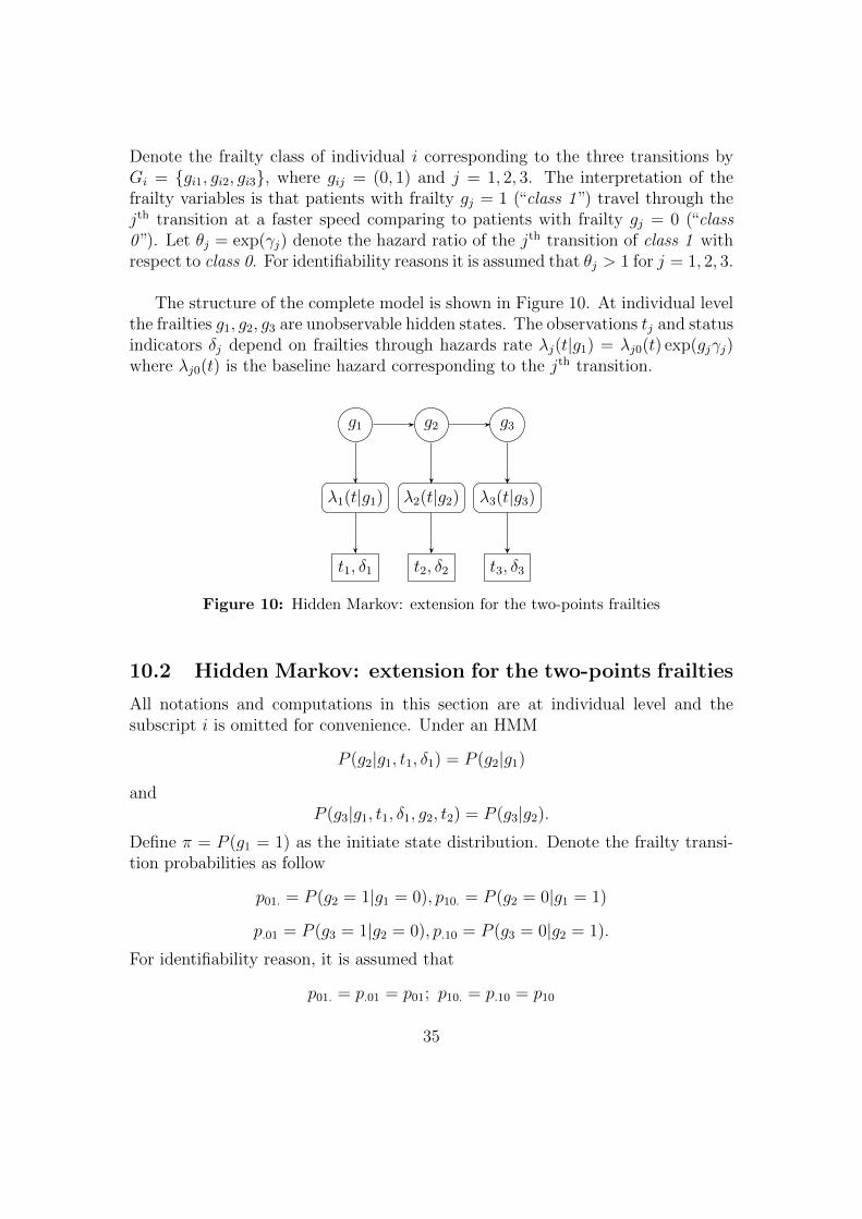
Denote the frailty class of individual i corresponding to the three transitions byGi = {gi1, gi2, gi3}, where gij = (0, 1) and j = 1, 2, 3. The interpretation of thefrailty variables is that patients with frailty gj = 1 (“class 1”) travel through thejth transition at a faster speed comparing to patients with frailty gj = 0 (“class0”). Let θj = exp(γj) denote the hazard ratio of the jth transition of class 1 withrespect to class 0. For identifiability reasons it is assumed that θj > 1 for j = 1, 2, 3.

The structure of the complete model is shown in Figure 10. At individual levelthe frailties g1, g2, g3 are unobservable hidden states. The observations tj and statusindicators δj depend on frailties through hazards rate λj(t|g1) = λj0(t) exp(gjγj)where λj0(t) is the baseline hazard corresponding to the jth transition.

g1 g2 g3

λ1(t|g1) λ2(t|g2) λ3(t|g3)

t1, δ1 t2, δ2 t3, δ3

Figure 10: Hidden Markov: extension for the two-points frailties

10.2 Hidden Markov: extension for the two-points frailties

All notations and computations in this section are at individual level and thesubscript i is omitted for convenience. Under an HMM

P (g2|g1, t1, δ1) = P (g2|g1)

andP (g3|g1, t1, δ1, g2, t2) = P (g3|g2).

Define π = P (g1 = 1) as the initiate state distribution. Denote the frailty transi-tion probabilities as follow

p01. = P (g2 = 1|g1 = 0), p10. = P (g2 = 0|g1 = 1)

p.01 = P (g3 = 1|g2 = 0), p.10 = P (g3 = 0|g2 = 1).

For identifiability reason, it is assumed that

p01. = p.01 = p01; p10. = p.10 = p10

35

g1 g2 g3 P (g1, g2, g3)

0 0 0 (1− π)(1− p01.)2

0 0 1 (1− π)(1− p01.)p.01

0 1 0 (1− π)p01.p.10

0 1 1 (1− π)p01.(1− p.10)1 0 0 πp10.(1− p.01)1 0 1 πp10.p.01

1 1 0 π(1− p10.)p.10

1 1 1 π(1− p10.)2

Table 4: Possible latent classes and corresponding joint probabilities

The joint probability P (g1, g2, g3) can be expressed as the product of initiate stateprobability and frailty transition probabilities. Table 4 lists all possible frailtysequences and corresponding probabilities.

More assumptions can be made to simplify the joint probabilities or for appli-cation purpose. For instance if it is assumed that p10. = p01. = 1 − P (g1 = g2)the resulting model can presents the correlation between transition 1 and tran-sition 2. If P (g1 = g2) = 0.5 the two transitions have correlation equal to 0; ifP (g1 = g2) > 0.5 the two transitions are positively correlated; if P (g1 = g2) < 0.5the two transitions are negatively correlated; P (g1 = g2) =1 and 0 indicates perfectpositive correlation and perfect negative correlation respectively.

In case that P (g1 = g2) = P (g2 = g3) = 1 the resulting model will be equivalentto a two-point mixture model with three frailties.

36

11 Work in Progress: EM Algorithm

The complete set of parameters (γ1, γ2, γ3, π, p10, p01) can be used to specify anHidden Markov two-point frailty model. To estimate these parameters, the Ex-pectation - Maximization (EM) algorithm [27] is very attractive due to the com-plete data likelihood structure. In this section, an EM algorithm for the hiddenMarkov two-point frailty model will be briefly introduced. Further developmentsfor implementation of the EM algorithm are still in progress.Denote by li;gi1,gi2,gi3 the likelihood for individual i conditional on the latent classGi defined before. The transition rates for individual i are given by the followingproportional hazards equations

λj;Gi= λj(tij) · γjgij

where j = 1, 2, 3.For an individual i the corresponding likelihood will be

li;gi1,gi2,gi3 = λ1;Gi(t1i)

δi1 exp(−Λ1;Gi(t1i))×

λ2;Gi(t2i)

δi2δi1 exp(−(Λ2;Gi(t2i)− Λ2;Gi

(t1i)))δi1×

λ3;Gi(t3i)

δi3δi2δi1 exp(−(Λ3;Gi(t3i)− Λ3;Gi

(t2i)− Λ3;Gi(t1i)))

δi2δi1 . (23)

Based on (23) for an individual i who never experience transition 1 (δi1 = 0), theconditional likelihood is given by

li;gi1,gi2,gi3 = exp(−Λ1;Gi(t1i)).

Similarly, for an individual i who has experienced transition 1 but never experiencetransition 2(δi1 = 1, δi2 = 0), the conditional likelihood is given by

li;gi1,gi2,gi3 = λ1;Gi(t1i) exp(−Λ1;Gi

(t1i)) exp(−(Λ2;Gi(t2i)− Λ2;Gi

(t1i)));

and for individual who has experience transition 1 and 2 but not transition 3, theconditional likelihood is given by

li;gi1,gi2,gi3 = λ1;Gi(t1i) exp(−Λ1;Gi

(t1i))×λ2;Gi

exp(−(Λ2;Gi(t2i)− Λ2;Gi

(t1i)))×exp(−(Λ3;Gi

(t3i)− Λ3;Gi(t2i)− Λ3;Gi

(t1i))). (24)

For all possible latent classes, we multiply the (cumulative) hazards with theappropriate hazard ratios. The complete log-likelihood is as follow

L(γ1, γ2, γ3, π, p10, p01) =∑n

i=1 log(P (G = 0, 0, 0)li;0,0,0 + P (G = 0, 0, 1)li;0,0,1

+ P (G = 0, 1, 0)li;0,1,0 + P (G = 0, 1, 1)li;0,1,1 + P (G = 1, 0, 0)li;1,0,0

+ P (G = 1, 0, 1)li;1,0,1 + P (G = 1, 1, 0)li;1,1,0 + P (G = 1, 1, 1)li;1,1,1).

37

EM algorithm

(i) E-step Start with the log-likelihood contribution for individual i.The conditional expectation of πi, given the data of individual i can be calcu-lated by

πi =P (G = 1, 0, 0)li,1,0,0 + P (G = 1, 0, 1)li,1,0,1∑

P (G)li,G

+P (G = 1, 1, 0)li,1,1,0 + P (G = 1, 1, 1)li,1,1,1∑

P (G)li,G,

where P (G) can be computed according to Table 4 and where li;g can becomputed based on (24).Similarly the conditional expectation of pi;01 given the data corresponding toindividual i can be calculated by

pi;01 =P (G = 0, 1, 0)li,0,1,0 + P (G = 0, 1, 1)li,0,1,1∑

P (G)li,G

+P (G = 1, 0, 1)li,1,0,1 + P (G = 0, 0, 1)li,0,0,1∑

P (G)li,G.

The conditional expectation of pi;10 is given as

pi;10 =P (G = 0, 1, 0)li,0,1,0 + P (G = 1, 1, 0)li,1,1,0∑

P (G)li,G

+P (G = 1, 0, 1)li,1,0,1 + P (G = 1, 0, 0)li,1,0,0∑

P (G)li,G.

(ii) M-step For the whole data set, calculate

π =1

n

n∑i=1

πi, p01 =1

n

n∑i=1

pi;01, andp10 =1

n

n∑i=1

pi;10

The hazard ratios γ1, γ2 and γ3 can be obtained separately by weighted Coxregressions for transition 1, 2, and 3 separately. The weights are employedhere because the latent classes are not observable and only their distributioncan be estimated. Let wj denote the vector of weights corresponding totransition j. The weights can be computed as

38

wij =

∑G:gj=1

P (G)li,G∑P (G)li,G

(iii) Repeat Iteration stops when the log-likelihood L(γ1, γ2, γ3, π, p10, p01)for subsequent iterations differs by less than a pre-specified small value.

39

12 Discussion

The focus of this thesis is to address the violation of the Markov or Markov renewalassumption in applications of multi-state models. Two statistical methods wereproposed. The first method was to include transition times as extra covariates,and the second was to introduce frailties under a Hidden Markov assumption.By employing a Cox regression model the influence of previous sojourn times onlater transitions can be estimated together with prognostic covariates effects. Ex-plicit analytical expression for the trajectory probabilities was developed for theextended Markov renewal model. The parameter estimates and correspondingbaseline hazards can be used to obtain prediction probabilities of future events.Confidence interval of the predicted probabilities can be obtained by simulations.The breast cancer data set was analyzed by employing an extended Markov renewalillness-death model (surgery, tumor recurrence and death). Prediction results be-tween the extended Markov renewal model and classic Markov renewal model havebeen compared.The merit of this extended model is the ability to deal with association betweentransition times. Illness-death model can be further extended to more complexmodel. However, the number of parameters to be estimated increases for morecomplex model, since the effects of sojourn time in each state on each later tran-sition needs to be estimated in the extended Markov renewal model.Another disadvantage of this approach is the computation-costly procedure forobtaining CIs by bootstrap sampling and simulation of trajectories through themulti-state model.Mathematical expression to estimate the predicted probabilities has been devel-oped in this dissertation. For Markov models, formulas based on Aalen and Jo-hansen‘s estimator and their standard errors are available (see [21]). For Markovrenewal models formulas for both non-parametric and semi-parametric estimatorsof the transition probabilities and corresponding standard error are recently avail-able (see Spitoni at al. [20]). More research need to be done to compute standarderror for the extended Markov model to provide a more efficient way of computingstandard errors for prediction estimates.It is important to investigate whether the transition time effects satisfies the Coxproportional assumption in applications of this extended Markov renewal model.The violation of Cox proportional assumption will lead to inconsistent estimateresults. There are two possible solutions to this problem. The first solution isto stratify patients by their sojourn times in each transitions. Unfortunately thismethod can be applicable only for simple model with a few transitions.Another solution is to introduce frailties which can deal with association betweentransitions as well as violation of Cox proportional hazard assumption. We pro-posed a combination of Hidden Markov model and two-point mixture frailty model.

40

One merit of the hidden Markov two-point frailty model is that it allows muchflexibility when modeling the latent frailty classes for patients population. It candeal with the violation of the Cox proportional hazard assumption as well. Oneshortcoming of this method might be the difficulty of estimating parameters in anefficient way. We proposed an EM algorithm to estimate this model. The resultsseem promising but more research need to be done.

41

References

[1] P. K. Andersen, N. Keiding, (2002),“Multi-state models for event historyanalysis”, Stat Methods Med Res 11: 91-115

[2] Hein Putter, Jos van der Hage, Geertruida H. de Bock, et al., (2006),“Esti-mation and prediction in a multi-state model for breast cancer”, BiometricalJournal 48: 366-380

[3] D. R. Cox, (1972). “Regression models and life tables (with discussion)”,Journal of the Royal Statistical Society B 34:187-220.

[4] T. M. Therneau, and P. M. Grambsch, (2001). “Modeling Survival Data:Extending the Cox Model”, Statistics for Biology and Health. New York:Springer.

[5] P. K. Andersen, L. S. Hansen, and N. Keiding, (1991). “Non- and semi-parametric estimation of transition probabilities from censored observationof a non-homogeneous Markov process”, Scandinavian Journal of Statistics18:153-16.

[6] P. K. Andersen, O. Brogan, R. D. Gill, N. Keiding (1993) Statistical ModelBased on Counting Processes, 2nd ed., Springer Series in Statistics, Springer.

[7] S. W. Lagakos, C. J. Sommer and M. Zelen (1978),“Semi-Markov models forpartially censored data”, Biometrika 65 (2): 311-317.

[8] R. D. Gill (1980),“Nonparametric Estimation Based on Censored Observa-tions of a Markov Renewal Process”, Z. Wahrscheinlichkeitstheorie verw.Gebiete 53: 97-116.

[9] R. L. Prentice, B. J. Williams and A. V. Peterson (1981),“On the regressionanalysis of multivariate failure time data”, Biometrika 68 (2): 373-379.

[10] D. M. Dabrowska, G. W. Sun, and M. M. Horowitz, (1994). “Cox regressionin a Markov renewal model: An application to the analysis of bone-marrowtransplant data”, Journal of the American Statistical Association 89:867-877.

[11] D. M. Dabrowska (1995). “Estimating of transition probabilities and boot-strap in a semiparametric Markov renewal model”,Nonparametric Statistics5:237-259.

[12] M. Fiocco, H. Putter and H. C. van Houwelingen (2008). “Reduced-rankproportional hazards regression and simulation-based prediction for multi-state models”, Statistics in Medicine 27:4340-4358.

42

[13] P. C. Clahsen, C. J. H. van de Velde, et al. (1996),“Improved Local Controland Disease-Free Survival After Perioperative Chemotherapy for Early-StageBreast Cancer: A European Organization for Research and Treatment ofCancer Breast Cancer Cooperative Group Study”, Journal of Clinical On-cology 14 (3): 745-753.

[14] J. A. van der Hage, C. J. H. van de Velde, J. P. Julien, et al. (2001),“Improvedsurvival after one course of perioperative chemotherapy in early breast cancerpatients: long-term results from the European Organization for Research andTreatment of Cancer (EORTC) Trial 10854”, European Journal of Cancer 37:2184-2193.

[15] H. Putter and H. C. van Houwelingen (2011),“Frailties in multi-state models:Are they identifiable? Do we need them?”, Statistical Methods in MedicalResearch 0(0): 1-18

[16] L. C. de Wreede, M. Fiocco, H. Putter (2010) ,“The mstate package for esti-mation and prediction in non- and semi-parametric multi-state and compet-ing risks models”,computer methods and programs in biomedicine 99:261-274.

[17] L. C. de Wreede,M. Fiocco,H. Putter (2011), “mstate: An R Package for theAnalysis of Competing Risks and Multi-State Models”, Journal of StatisticalSoftware, 38(7): 1-30.

[18] H. Putter, M. Fiocco and R. B. Geskus (2007), “Tutorial in biostatistics:Competing risks and multi-state models”, Statistics in Medicine 26:2389-2430.

[19] O. O. Aalen, S. Johansen (1978), “An empirical transition matrix for non-homogeneous Markov chains based on censored observations”, ScandinavianJournal of Statistics 5:141-150.

[20] C. Spitoni, M. Verduijn, H. Putter (2012), “Estimation and Asymptotic The-ory for Transition Probabilities in Markov Renewal Multi-State Models”, TheInternational Journal of Biostatistics 8(1), Art. 23

[21] O. O. Aalenand and S. Johansen(1987).“Empirical transition matrix for non-homogeneous Markov-chains based on censored observations”. Scand J Stat5: 141-150.

[22] M. Bhattacharya and J. P. Klein (2005) “A random effects model for multi-state survival analysis with application to bone marrow transplants”, MathBiosci 2005 194: 37-48.

43

[23] A. M. F. Yen , T. H. H. Chen, S. W. Duffy and C. D. Chen (2010)“ Incorpo-rating frailty in a multi-state model: application to disease natural historymodelling of adenoma-carcinoma in the small bowel”, Stat Methods Med Res2010 19: 529-546.

[24] P. Hougaard (1984), “Life table methods for heterogeneous populations”,Biometrika 71: 75-83

[25] H. Putter and H. C. van Houwelingen, Frailties in multi-state models: Arethey identifiable? Do we need them? Statistical Methods in Medical Re-search0(0): 1-18

[26] L. R. Rabiner and B. H. Juang (1986),“ An Introduction to hidden Markovmodels”, iEEE Acoust, Speech, Signal Processing Mag. 3(1): 4-16

[27] A. P. Dempster, N. M. Laird, and D. B. Rubin (1977), ‘Maximum likelihoodfrom incomplete data via the em algorithm’,Journal of the Royal StatisticalSociety/ Series B (Methodological) 39(1): 1-38.

44

A Functions Defined for the Analysis

1 g e t l e v e l <−f unc t i on ( covs , data ) { #data i s the o r i g i n a l data , covsi s the covs used to expand

2 i f (mean( covs %in% colnames ( data ) ) !=1){ stop ( ”Found :undef ined v a r i a b l e ”) }

3 e l s e { temp<−as . l i s t ( data [ , colnames ( data ) %in% covs ] )4 sapply ( temp , l e v e l s )5 }6 }7

8 newprep<−f unc t i on (y , covs , f i t , l v l s ){#covs i s the vec to r covswhen expand the data

9 i f ( nco l ( y ) != length ( covs ) ) { stop ( ”The number o f c o v a r i a t e sdo not match ”) }

10 e l s e { y<−y [ , order ( colnames ( y ) ) ]11 covs<−s o r t ( covs )12 i f (sum( colnames ( y ) != covs )>0){ stop ( ”The c o v a r i a t e

names do not match ”) }13 e l s e { beta . names<−s o r t ( names ( summary( f i t ) $ coe f [ , 1 ] ) )14 n . trans<−l ength ( f i t $ x l e v e l s [ [ 1 ] ] )15 newdata<−matrix (0 , n . t rans ∗nrow ( y ) , l ength ( beta .

names ) )16 colnames ( newdata )<−beta . names#c r e a t e a matrix

with 0 s17

18 f o r ( i in 1 : nrow ( y ) ) {19 f o r ( j in 1 : nco l ( y ) ) {20 temp<−paste ( covs [ j ] , sep =””) #e x t r a c t name21 temp . l<− l v l s [ [ temp ] ]22 i f ( l ength ( temp . l )>0) {temp .dummy<− which ( temp

. l==y [ i , j ] )−1 #charac t e r23 i f ( l ength ( temp .dummy)==0){ stop ( ”undef ined

v a r i a b l e ”) }24 i f ( temp .dummy>0){ inx<−grep ( temp , beta . names ) [ 1 : n .

t rans ]+(temp .dummy−1)∗n . t rans25 diag ( newdata [ ( i −1)∗n . t rans +(1:n . t rans ) , inx ] )

<−126 }27 }# the case cov i s a c a t e g o r i c a l28 e l s e { inx<−grep ( temp , beta . names ) [ 1 : n . t rans ]29 diag ( newdata [ ( i −1)∗n . t rans +(1:n . t rans ) ,

inx ] )<−y [ i , j ] }

45

30 #numeric31 }32

33 }34 data . frame ( t rans=rep ( 1 : n . trans , nrow ( y ) ) , newdata )35

36

37

38 }39

40 }41

42

43 }44

45 S . t<−f unc t i on ( time , S) {46 t<−S [ , 1 ]47 s<−S [ , 2 ]48 n<−l ength ( time )49 r e s u l t <−numeric (n)50 f o r ( i in 1 : n ) {51 i f ( time [ i ]<min ( t ) ) { r e s u l t [ i ]<−1}52 e l s e { i f ( time [ i ]>max( t ) ) { r e s u l t [ i ]<−min (S) }53 e l s e r e s u l t [ i ]<− t a i l (S [ t<=time [ i ] ] , 1 )54 }}55 r e s u l t }56 pred ic t1<−f unc t i on ( f i t , newdata , t , bt , r ) {57 newdata$trans<−NULL58 beta . a l l <−summary( f i t ) $ coe f [ , 1 ]59 i f ( i s . n u l l ( bt ) ) {beta . t<−060 beta<−beta . a l l [ o rder ( names ( beta . a l l ) ) ]}61 e l s e { i f (sum( bt %in% names ( beta . a l l ) )==0) stop ( ”undeined time

v a r i a b l e ”)62 e l s e {beta . t<−beta . a l l [ bt ]63 beta<−beta . a l l [ names ( beta . a l l ) !=bt ]64 beta<−beta [ order ( names ( beta ) ) ]65 newdata<−newdata [ , colnames ( newdata ) !=bt ]66 }67 }68

69 i f (mean( names ( beta )==names ( newdata ) ) !=1){ stop ( ”undef inedv a r i a b l e ”) }

70 e l s e {ZB<−as . matrix ( newdata )%∗%beta

46

71 f i t . base<−s u r v f i t ( f i t )72 s t ra ta<− f i t . ba s e$ s t r a ta73 inx<−c (cumsum( s t r a t a )−s t ra ta , sum( s t r a t a ) )74 ###############b a s e l i n e

#######################################75 H. base l i n e<−sapply ( 1 : 3 , f unc t i on ( x )76 cbind ( f i t . base$time [ ( inx [ x ]+1) : inx [ x +1 ] ] ,77 −l og ( f i t . base$surv [ ( inx [ x ]+1) : inx [ x +1 ] ] ) ) )78 time<−H. b a s e l i n e [ [ 3 ] ] [ , 1 ]79 ################semi−Markiv###############Harzad

####################80 H. Zr<−H. b a s e l i n e [ [ 3 ] ] [ , 2 ] ∗ exp (ZB [ 3 ] ) ∗exp ( r ∗ beta . t )81 #####################S22 stay in s t a t e 2##########

t r a n s i t i o n 3 f r e e##82 S22<−exp(−H. Zr )83 ####################P23 from s t a t e 2 to 3##########

t r a n s i t i o n 3#######84 P23<−1−S2285

86

87 r e s u l t <− l i s t ( probs=cbind ( time , S22 , S23 ) , hazards=H. Zr )88 colnames ( r e s u l t [ [ 1 ] ] ) =c ( ”time ” , ”P22 ” , ”P23 ”)89 re turn ( r e s u l t )90 }91

92 }93 pred ic t0<−f unc t i on ( f i t , newdata , t , bt ) {94 newdata$trans<−NULL95 beta . a l l <−summary( f i t ) $ coe f [ , 1 ]96 i f ( i s . n u l l ( bt ) ) {beta . t<−097 beta<−beta . a l l [ o rder ( names ( beta . a l l ) ) ]}98 e l s e { i f (sum( bt %in% names ( beta . a l l ) )==0) stop ( ”undeined time

v a r i a b l e ”)99 e l s e {beta . t<−beta . a l l [ bt ]

100 beta<−beta . a l l [ names ( beta . a l l ) !=bt ]101 beta<−beta [ order ( names ( beta ) ) ]102 newdata<−newdata [ , colnames ( newdata ) !=bt ]103 }104 }105

106 i f (mean( names ( beta )==names ( newdata ) ) !=1){ stop ( ”undef inedv a r i a b l e ”) }

107 e l s e {ZB<−as . matrix ( newdata )%∗%beta

47

108 f i t . base<−s u r v f i t ( f i t )109 s t ra ta<− f i t . ba s e$ s t r a ta110 inx<−c (cumsum( s t r a t a )−s t ra ta , sum( s t r a t a ) )111 ###############b a s e l i n e

#######################################112 H. base l i n e<−sapply ( 1 : 3 , f unc t i on ( x )113 cbind ( f i t . base$time [ ( inx [ x ]+1) : inx [ x +1 ] ] ,114 −l og ( f i t . base$surv [ ( inx [ x ]+1) : inx [ x +1 ] ] ) ) )115 ################semi−Markiv###############Harzad

####################116 H. Z<−sapply ( 1 : 3 , f unc t i on ( x ) cbind (H. b a s e l i n e [ [ x ] ] [ , 1 ] ,H

. b a s e l i n e [ [ x ] ] [ , 2 ] ∗ exp (ZB[ x ] ) ) )117 #####################S22 stay in s t a t e 2##########

t r a n s i t i o n 3 f r e e##118 S22<−cbind (H. Z [ [ 3 ] ] [ , 1 ] , exp(−H. Z [ [ 3 ] ] [ , 2 ] ) )119 ####################P23 from s t a t e 2 to 3##########

t r a n s i t i o n 3#######120 #P23<−1−S22121 #####################S11 stay in s t a t e 1##############

DFS############122 H1 . Z<−H. Z [ [ 1 ] ] [ , 2 ]123 H2 . Z<−H. Z [ [ 2 ] ] [ , 2 ]124 dH1 . Z<−c (H1 . Z [ 1 ] , d i f f (H1 . Z) )125 dH2 . Z<−c (H2 . Z [ 1 ] , d i f f (H2 . Z) )126 time1<−H. Z [ [ 1 ] ] [ , 1 ]127 inx<−time1>=t & (dH1 . Z!=0 |dH2 . Z!=0)128 time . t<−time1 [ inx ]129 dH1 . Zt<−dH1 . Z [ inx ]130 dH2 . Zt<−dH2 . Z [ inx ]131 S11 . Zt<−exp(−cumsum(dH1 . Zt+dH2 . Zt ) )132 #################P13 from s t a t e 1 to s t a t e 3#######

t r a n s i t i o n 2######133 P13 . Zt<−cumsum(dH2 . Zt∗S11 . Zt )134 #################P122 from s t a t e 1 to s t a t e 2 and stay

###t r a n s i t i o n 1#135 P122 . Zt<−P123 . Zt<−rep (NA, sum( inx ) )136 f o r ( i in 1 : sum( inx ) ) {137 v<−time . t [ 1 : i ]138 dtime<−time . t [ i ]−v139 S22 . dtime.0<−S . t ( dtime , S22 )140 S22 . dtime . v<−S22 . dtime .0ˆ exp ( v∗ beta . t )141 P122 . Zt [ i ]<−sum(dH1 . Zt [ 1 : i ]∗ S11 . Zt [ 1 : i ]∗ S22 . dtime . v )

48

142 P123 . Zt [ i ]<−sum(dH1 . Zt [ 1 : i ]∗ S11 . Zt [ 1 : i ]∗(1−S22 . dtime .v ) )

143 }144

145 r e s u l t <− l i s t ( probs=cbind ( time . t , S11 . Zt , P122 . Zt , P123 . Zt ,P13 . Zt ) , hazards=H. Z)

146 colnames ( r e s u l t [ [ 1 ] ] ) =c ( ”time ” , ”P11 ” , ”P122 ” , ”P123 ” , ”P13”)

147 colnames ( r e s u l t $ h a z a r d s [ [ 1 ] ] ) =c ( ”time ” , ” t rans1 ”)148 colnames ( r e s u l t $ h a z a r d s [ [ 2 ] ] ) =c ( ”time ” , ” t rans2 ”)149 colnames ( r e s u l t $ h a z a r d s [ [ 3 ] ] ) =c ( ”time ” , ” t rans3 ”)150 re turn ( r e s u l t )151 }152

153 }154 pred i c t<−f unc t i on ( f i t , newdata , t , bt ) {155 i f ( newdata$Tstart [ 2 ] ! = 0 ) { r<−newdata$Tstart [ 2 ]156 r e s u l t <−pr ed i c t 1 ( f i t , newdata , t , bt , r ) }157 e l s e { r e s u l t <−pr ed i c t 0 ( f i t , newdata , t , bt ) }158 re turn ( r e s u l t )159 }160 p lo t . p red i c t<−f unc t i on ( l i s 0 , c o l s=c ( ”red ” , ”orange ” , ” l i g h t g r e e n

” , ” l i g h t b l u e ”) ) {161 x<− l i s 0 [ [ 1 ] ] [ , 1 ]162 y1<−rep (1 , l ength ( x ) )163 y2<−1− l i s 0 [ [ 1 ] ] [ , 5 ]164 p lo t (x , y2 , xl im=c (0 ,max( x ) ) , yl im=c (0 , 1 ) , type=”s ” , xlab=”Time

a f t e r surgery ” ,165 ylab=”P r o b a b i l i t y ”)166 polygon ( c (x , rev ( x ) ) , c ( y2 , rev ( y1 ) ) , c o l=c o l s [ 1 ] )167 y3<−y2− l i s 0 [ [ 1 ] ] [ , 4 ]168 l i n e s (x , y3 , type=”s ”)169 polygon ( c (x , rev ( x ) ) , c ( y3 , rev ( y2 ) ) , c o l=c o l s [ 2 ] )170 y4<−y3− l i s 0 [ [ 1 ] ] [ , 3 ]171 l i n e s (x , y4 , type=”s ” , c o l =”black ”)172 polygon ( c (x , rev ( x ) ) , c ( y4 , rev ( y3 ) ) , c o l=c o l s [ 3 ] )173 y5<−rep (0 , l ength ( x ) )174 polygon ( c (x , rev ( x ) ) , c ( y4 , rev ( y5 ) ) , c o l=c o l s [ 4 ] )175 }176 prob . pred i c t<−f unc t i on ( time , probs ) {177 temp<−t a i l ( probs [ probs [ ,1 ] <=6 , ] ,1 )178 temp<−c ( temp [ , 2 : 3 ] , temp [ ,4 ]+ temp [ , 5 ] )179 names ( temp )<−c ( ”P1 ” , ”P2 ” , ”P3 ”)

49

180 temp181 }182 haz<−f unc t i on ( f i t , newdata ) {183 beta<−summary( f i t ) $ coe f [ , 1 ]184 beta<−beta [ order ( names ( beta ) ) ]185 ############c o e f f i c i e n t##################186 newdata$trans<−NULL187 ZB<−as . matrix ( newdata )%∗%beta188 #############b a s e l i n e####################189 f i t . base<−s u r v f i t ( f i t )190 s t ra ta<− f i t . ba s e$ s t r a ta191 inx<−c (cumsum( s t r a t a )−s t ra ta , sum( s t r a t a ) )192 H. base l i n e<−sapply ( 1 : 3 , f unc t i on ( x )193 cbind ( f i t . base$time [ ( inx [ x ]+1) : inx [ x +1 ] ] ,194 −l og ( f i t . base$surv [ ( inx [ x ]+1) : inx [ x +1 ] ] ) ) )195 ############hazard#########################196 H. Z<−sapply ( 1 : 3 , f unc t i on ( x ) cbind (H. b a s e l i n e [ [ x ] ] [ , 1 ] ,H.

b a s e l i n e [ [ x ] ] [ , 2 ] ∗ exp (ZB[ x ] ) , x ) )197 hazard<−rbind (H. Z [ [ 1 ] ] , H. Z [ [ 2 ] ] , H. Z [ [ 3 ] ] )198 hazard<−as . data . frame ( hazard )199 colnames ( hazard )<−c ( ”time ” , ”Haz ” , ” t rans ”)200 re turn ( hazard )201 }

50

B Codes for the Analysis

1 ###############new data#######################2 covs<−c ( ” per iop ” , ”surgery ” , ” t u s i ” , ”nodal ” , ”age50 ” ,

”adjchem ”)3 ( l v l s <−g e t l e v e l ( covs , bc . long ) )4 y<−data . frame ( per iop =”no per iop chemo ” , surgery =”mastectomy with

RT” , t u s i =”>5 cm” ,5 nodal=”node p o s i t i v e ” , adjchem=”no adj chemo ” ,6 age50=”<=50”)7 f i t <−coxph ( Surv ( time , s t a t u s ) ˜.− t rans+s t r a t a ( t rans ) , bc . long [ ,− c

( 1 : 3 , 6 , 9 : 1 5 ) ] )8 newdata<−newprep (y , covs , f i t , l v l s )9 ###############p r e d i t c t######################

10 r e s u l t s <−p r e d i c t ( f i t , newdata , t =0,bt=”Tstart ”)11 ###############plo t##########################12 p lo t . p r e d i c t ( r e s u l t s )13 l egend ( ” bot tomle f t ” , c ( ”Surgery to Death ” , ”Surgery to Rec to

Death ” , ”Recurrence ” , ”DFS”) ,14 lwd=2, c o l=c ( ”red ” , ”orange ” , ” l i g h t g r e e n ” , ” l i g h t b l u e ”) , cex

=0.6)15

16 ############se###############################17 tmat <− t rans . i l l d e a t h ( )18 M=10019 tvec=r e s u l t s $ p r o b s [ , 1 ]20 h i s to ry<− l i s t ( s t a t e =1, time =0, t s t a t e s=c (0 , 0 , 0 ) )21 theta<−f unc t i on ( data ) {22 dat<−data [ ,− c ( 1 : 3 , 6 , 9 : 1 5 ) ]23 f i t <−coxph ( Surv ( time , s t a t u s ) ˜.− t rans+s t r a t a ( t rans ) , dat )24 Haz<−haz ( f i t , newdata )25 bt<−summary( f i t ) $ coe f [ , 1 ] [ ” Tstart ”]26 beta . s ta te<−matrix (0 , 3 , 3 )27 beta . s t a t e [1 ,2]<−bt28 res<−mssample (Haz , t rans=tmat , c l o ck =”r e s e t ” , h i s t o r y=hi s to ry ,

beta . s t a t e=beta . s ta te , tvec=tvec ,M=M)29 c ( as . matrix ( r e s [ , −1 ] ) )30

31 }32 theta ( bc . long )33 theta2<−f unc t i on ( data ) {34 f i t 0 <−coxph ( Surv ( time , s t a t u s ) ˜.− t rans+s t r a t a ( t rans ) , data [ ,− c

( 1 : 3 , 6 , 9 : 1 5 ) ] )

51

35 temp0<−p r e d i c t ( f i t 0 , newdata , t =5,bt=”Tstart ”)36 probs<−temp0$probs37 temp<−c ( probs [ , 2 : 5 ] )38 re turn ( temp )39 }40 msboot ( theta2 , bc . long ,B=1, id=”id ”)41

42 theta2<−f unc t i on ( data ) {43 f i t 0 <−coxph ( Surv ( time , s t a t u s ) ˜.− t rans+s t r a t a ( t rans ) , data [ ,− c

( 1 : 3 , 6 , 9 : 1 5 ) ] )44 res0<−p r e d i c t ( f i t 0 , newdata , t =12, bt=”Tstart ”)45 probs<−re s0$probs46 temp<−c ( as . matrix ( probs ) )47 re turn ( temp )48 }49

50 p lo t . p r e d i c t ( r e s u l t s )51 l i n e s ( r e s [ , 1 ] , r e s [ , 2 ]+ r e s [ , 3 ] , c o l =2)52 l i n e s ( r e s [ , 1 ] , r e s [ , 2 ] , c o l =2)53 theta2<−f unc t i on ( data , t rans=tmat ) {54 f i t <−coxph ( Surv ( time , s t a t u s ) ˜.− t rans+s t r a t a ( t rans ) , data [ ,− c

( 1 : 3 , 6 , 9 : 1 5 ) ] )55 r e s u l t s <−p r e d i c t ( f i t , newdata , t =0,bt=”Tstart ”)56 c ( as . matrix ( r e s u l t s $ p r o b s [ , 2 : 5 ] ) )57 }58 res<−msboot ( theta , bc . long ,B=5, id=”id ”)59

60

61 tmat <− t rans . i l l d e a t h ( )62 M=1063 tvec=664 h i s to ry<− l i s t ( s t a t e =1, time =0, t s t a t e s=c (0 , 0 , 0 ) )65 theta<−f unc t i on ( data ) {66 dat<−data [ ,− c ( 1 : 3 , 6 , 9 : 1 5 ) ]67 f i t <−coxph ( Surv ( time , s t a t u s ) ˜.− t rans+s t r a t a ( t rans ) , dat )68 Haz<−haz ( f i t , newdata )69 bt<−summary( f i t ) $ coe f [ , 1 ] [ ” Tstart ”]70 beta . s ta te<−matrix (0 , 3 , 3 )71 beta . s t a t e [1 ,2]<−bt72 res<−mssample (Haz , t rans=tmat , c l o ck =”r e s e t ” ,73 h i s t o r y=hi s to ry , beta . s t a t e=beta . s ta te , tvec=tvec

,M=M)74 c ( as . matrix ( r e s [ , −1 ] ) )

52

75 }76 res<−msboot ( theta , bc . long ,B=50, id=”id ”)77 LCI<−apply ( res , 1 , f unc t i on ( x ) q u a n t i l e (x , probs =0.025) )78 UCI<−apply ( res , 1 , f unc t i on ( x ) q u a n t i l e (x , probs =0.975) )79 CI<−cbind (LCI , UCI)80

81 ##########Extended Markov renewal vs . Markov renewal###########82 f i t 2 <−coxph ( Surv ( time , s t a t u s ) ˜.− t rans+s t r a t a ( t rans )−Tstart , bc .

long [ ,− c ( 1 : 3 , 6 , 9 : 1 5 ) ] )83 newdata2<−newdata84 newdata2$Tstart<−NULL85 r e s u l t s 2 . b<−p r e d i c t ( f i t 2 , newdata2 , t =0,bt=NULL)86 r e s u l t s 2 . a<−p r e d i c t ( f i t 2 , newdata2 , t =2,bt=NULL)87 r e s u l t s . b<−p r e d i c t ( f i t , newdata , t =0,bt=”Tstart ”)88 r e s u l t s . a<−p r e d i c t ( f i t , newdata , t =2,bt=”Tstart ”)89 par ( mfrow=c (1 , 1 ) )90 p lo t . p r e d i c t ( r e s u l t s 2 . a )91 l egend ( ” bot tomle f t ” , c ( ”Surgery to Death ” , ”Surgery to Rec to

Death ” , ”Recurrence ” , ”DFS”) ,92 lwd=2, c o l=c ( ”red ” , ”orange ” , ” l i g h t g r e e n ” , ” l i g h t b l u e ”) , cex

=0.75)93

94 p lo t . p r e d i c t ( r e s u l t s . b )95 l egend ( ” bot tomle f t ” , c ( ”Surgery to Death ” , ”Surgery to Rec to

Death ” , ”Recurrence ” , ”DFS”) ,96 lwd=2, c o l=c ( ”red ” , ”orange ” , ” l i g h t g r e e n ” , ” l i g h t b l u e ”) , cex

=0.75)97

98 p lo t . p r e d i c t ( r e s u l t s 2 . a )99 l egend ( ” bot tomle f t ” , c ( ”Surgery to Death ” , ”Surgery to Rec to

Death ” , ”Recurrence ” , ”DFS”) ,100 lwd=2, c o l=c ( ”red ” , ”orange ” , ” l i g h t g r e e n ” , ” l i g h t b l u e ”) , cex

=0.75)101 p lo t . p r e d i c t ( r e s u l t s . a )102 l egend ( ” bot tomle f t ” , c ( ”Surgery to Death ” , ”Surgery to Rec to

Death ” , ”Recurrence ” , ”DFS”) ,103 lwd=2, c o l=c ( ”red ” , ”orange ” , ” l i g h t g r e e n ” , ” l i g h t b l u e ”) , cex

=0.75)104

105

106

107 ############For pa t i en t c########################108 r e s u l t s . c<−pr ed i c t 1 ( f i t , newdata , t =5,bt=”Tstart ” , r =0.5)

53

109 r e s u l t s . c2<−pr ed i c t 1 ( f i t , newdata , t =5,bt=”Tstart ” , r=1)110 r e s u l t s . c3<−pr ed i c t 1 ( f i t , newdata , t =5,bt=”Tstart ” , r=2)111 r e s u l t s . c4<−pr ed i c t 1 ( f i t , newdata , t =5,bt=”Tstart ” , r=4)112

113 p lo t ( r e s u l t s . c [ , 1 : 2 ] , yl im=c (0 , 1 ) , type=”l ” , xlim=c ( 5 , 1 2 . 4 ) , c o l =1,lwd=2,

114 xlab=”Time a f t e r surgery ” , ylab=”Surv iva l Pr o ba b i l i t y ”)115 l i n e s ( r e s u l t s . c2 [ , 1 : 2 ] , type=”l ” , c o l =2, lwd=2)116 l i n e s ( r e s u l t s . c3 [ , 1 : 2 ] , type=”l ” , c o l =3, lwd=2)117 l i n e s ( r e s u l t s . c4 [ , 1 : 2 ] , type=”l ” , c o l =4, lwd=2)118 l egend ( ” to p r i g h t ” , c ( ”Reccurence a f t e r 0 .5 year ” , ”Reccurence

a f t e r 1 year ” ,119 ”Reccurence a f t e r 2 years ” , ”Reccurence

a f t e r 4 years ”) ,120 lwd=2, c o l =1:4)121

122 r e s u l t s 2 . c<−pr ed i c t 1 ( f i t 2 , newdata2 , t =5,bt=NULL, r =0.5)123 r e s u l t s 2 . c2<−pr ed i c t 1 ( f i t 2 , newdata2 , t =5,bt=NULL, r=1)124 r e s u l t s . c3<−pr ed i c t 1 ( f i t , newdata , t =5,bt=”Tstart ” , r=2)125 p lo t ( r e s u l t s 2 . c [ , 1 : 2 ] , yl im=c (0 , 1 ) , type=”l ” , xlim=c ( 5 , 1 2 . 4 ) , c o l

=1, lwd=3,126 xlab=”Time a f t e r surgery ” , ylab=”Surv iva l Pr o ba b i l i t y ”)127 l i n e s ( r e s u l t s 2 . c2 [ , 1 : 2 ] , type=”l ” , c o l =2)128

129 ########CIs by s imu la t i on##########################130

131 res2<−msboot ( theta2 , bc . long ,B=500 , id=”id ”)132 save ( res , f i l e =”boot . a l l t i m e . M100 . B500 ”)133 load ( ”boot . a l l t i m e . M100 . B500 ”)134 se<−apply ( res , 1 , sd )135 se<−matrix ( se , nco l =3)136 LCI<−apply ( res , 1 , f unc t i on ( x ) q u a n t i l e (x , probs =0.025) )137 LCI<−matrix (LCI , nco l =3)138 UCI<−apply ( res , 1 , f unc t i on ( x ) q u a n t i l e (x , probs =0.975) )139 UCI<−matrix (UCI , nco l =3)140 head (UCI)141 tvec<−r e s u l t s . b [ [ 1 ] ] [ , 1 ]142 p lo t ( r e s u l t s . b [ [ 1 ] ] [ , 1 ] , r e s u l t s . b [ [ 1 ] ] [ , 2 ] , type=”l ” , ylim=c (0 , 1 )

,143 xlab=”Time a f t e r surgery ” , ylab=”P ro ba b i l i t y ” , main=”DFS”)144 l i n e s ( tvec , LCI [ , 1 ] , type=”l ” , l t y =3)145 l i n e s ( tvec , UCI [ , 1 ] , type=”l ” , l t y =3)146

54

147 p lo t ( r e s u l t s . b [ [ 1 ] ] [ , 1 ] , r e s u l t s . b [ [ 1 ] ] [ , 3 ] , type=”l ” , ylim=c (0 , 1 ),

148 xlab=”Time a f t e r surgery ” , ylab=”P ro ba b i l i t y ” , main=”Reccurence ”)

149 l i n e s ( tvec , LCI [ , 2 ] , type=”l ” , l t y =3)150 l i n e s ( tvec , UCI [ , 2 ] , type=”l ” , l t y =3)151

152 p lo t ( r e s u l t s . b [ [ 1 ] ] [ , 1 ] , ( r e s u l t s . b [ [ 1 ] ] [ , 4 ] + r e s u l t s . b [ [ 1 ] ] [ , 5 ] ), type=”l ” , yl im=c (0 , 1 ) ,

153 xlab=”Time a f t e r surgery ” , ylab=”P ro ba b i l i t y ” , main=”Death ”)154 l i n e s ( tvec , LCI [ , 3 ] , type=”l ” , l t y =3)155 l i n e s ( tvec , UCI [ , 3 ] , type=”l ” , l t y =3)156

157

158 f i t <−coxph ( Surv ( time , s t a t u s ) ˜.− t rans+s t r a t a ( t rans ) , bc . long [ ,− c( 1 : 3 , 6 , 9 : 1 5 ) ] )

159

160

161

162

163 ############For pa t i en t c########################164 r e s u l t s . c<−pr ed i c t 1 ( f i t , newdata , t =5,bt=”Tstart ” , r =0.5)165 r e s u l t s . c2<−pr ed i c t 1 ( f i t , newdata , t =5,bt=”Tstart ” , r=1)166 r e s u l t s . c3<−pr ed i c t 1 ( f i t , newdata , t =5,bt=”Tstart ” , r=2)167 r e s u l t s . c4<−pr ed i c t 1 ( f i t , newdata , t =5,bt=”Tstart ” , r=4)168

169 p lo t ( r e s u l t s . c [ , 1 : 2 ] , yl im=c (0 , 1 ) , type=”l ” , xlim=c ( 5 , 1 2 . 4 ) , c o l =1)170 l i n e s ( r e s u l t s . c2 [ , 1 : 2 ] , type=”l ” , c o l =2)171 l i n e s ( r e s u l t s . c3 [ , 1 : 2 ] , type=”l ” , c o l =3)172 l i n e s ( r e s u l t s . c4 [ , 1 : 2 ] , type=”l ” , c o l =4)173

174

175 r e s u l t s 2 . c<−pr ed i c t 1 ( f i t 2 , newdata2 , t =5,bt=NULL, r =0.5)176 r e s u l t s 2 . c2<−pr ed i c t 1 ( f i t 2 , newdata2 , t =5,bt=NULL, r=1)177 r e s u l t s . c3<−pr ed i c t 1 ( f i t , newdata , t =5,bt=”Tstart ” , r=2)178 p lo t ( r e s u l t s 2 . c [ , 1 : 2 ] , yl im=c (0 , 1 ) , type=”l ” , xlim=c ( 5 , 1 2 . 4 ) , c o l

=1)179 l i n e s ( r e s u l t s 2 . c2 [ , 1 : 2 ] , type=”l ” , c o l =2)180

181 setwd (”/ Users / songoku/Documents/Master Thes i s /Syntax ”)182 load ( ” r e s u l t s ”)183 pr<−r e s u l t s $ p r o b s

55

184 p lo t ( pr [ , 1 ] , pr [ , 2 ] , lwd=2, type=”l ” , xlab=”P r o b a b i l i t y ” , ylab=”time a f t e r surgery ”)

185 l i n e s ( pr [ , 1 ] , pr [ , 2 ]+ pr [ , 3 ] , lwd=2, type=”l ”)186 l i n e s ( pr [ , 1 ] , pr [ , 2 ]+ pr [ , 3 ]+ pr [ , 4 ] , lwd=2, type=”l ”)187 pr2<−r e s u l t s 2 . a$probs188 l i n e s ( pr2 [ , 1 ] , pr2 [ , 2 ] , lwd=2, type=”l ” , c o l =2)189 l i n e s ( pr2 [ , 1 ] , pr2 [ , 2 ]+ pr2 [ , 3 ] , lwd=2, type=”l ” , c o l =2)190 l i n e s ( pr2 [ , 1 ] , pr2 [ , 2 ]+ pr2 [ , 3 ]+ pr2 [ , 4 ] , lwd=2, type=”l ” , c o l =2)191 l egend ( ” bot tomle f t ” , lwd=2,c ( ”Extended Markov renewal ” , ”Markov

renewal ”) , c o l =1:2 , cex =0.75)

56