arX

iv:h

ep-p

h/02

0509

5v2

7 S

ep 2

002

Color-SU(3)-Ginzburg-Landau Effective Potential for Order

Parameter with 3× 3 Symmetry

E. Nakano, T. Suzuki and H. Yabu

Department of Physics, Tokyo Metropolitan University, 1-1 Minami-Ohsawa, Hachioji, Tokyo

192-0397, Japan

(November 10, 2018)

Abstract

Ginzburg-Landau effective potential is studied for the order parameter that

transforms in the (3, 3) representation under the color SU(3) group. All

the SU(3) invariant terms to the fourth-order of the order parameter are

classified and the effective potential is constructed in its most general form.

The conditions which stabilize the condensed phases are also obtained. As

applications, the classification of the condensed phase is discussed in some

special cases and the Higgs phenomenon associated with symmetry breaking

is studied by introducing a coupling to the gauge boson.

Typeset using REVTEX

1

I. INTRODUCTION

Recently, quark-pair condensation phenomena (color-superconductor) have received

much interest in the high-density nuclear physics [1,2].

In a high-density quark matter, quarks make a correlated Cooper pair due to the at-

tractive one-gluon-exchange [3,6] or instanton-induced interactions [4]. A lot of studies have

been done for physical properties of color superconductors on the basis of the QCD-inspired

models [5–9].

From the symmetry point of view, the color-superconductor is characterized by the spon-

taneous symmetry breaking of the color SUC(3) symmetry. Let’s consider the quark field

operator qα(r) with the color index α = 1, 2, 3 (other degrees of freedom, flavors and spins,

are represented, e.g., as q = u↑). They transform as a vector (the 3-representation) under

the SUC(3) transformation. (Irreducible representations of SU(3) are denoted by their di-

mensions, e.g. 1, 3, 3∗, etc.) The color-superconductor is a long-range ordered state, the

order parameter of which is a two-body one: Ψα,β(r) = 〈qα(r)q′β(r)〉. It is a second-rank

tensor under SUC(3) with nine components, which makes a reducible 3× 3-representation.

Different from the systems with a scalar order parameter (metal superconductor, super-

fluid 4He, etc.), a variety of symmetry-breaking patterns shows up in the condensed states

with the tensor order parameter. A typical example is the superfluid 3He, where, due to the

p-wave nature of the Cooper pair, the order parameter has a tensor-type spin structure, Φi,j

(i, j = 1, 2, 3); it transforms as the 3 × 3-representation in the orbital and spin rotations

G = SOL(3)⊗SOS(3) (also with the gauge U(1) symmetry). Corresponding to several sym-

metry breaking patterns, many different condensed phases show up in the superfluid 3He:

A-phase (H = (S2 × SO(3))/Z2), B-phase (RB = S1 × SOa(3)), and so on. As discussed

later, such a phase structure should exist also for the SU(3)-3 × 3-type order parameter,

and it is very interesting to study the structures for such a novel symmetry breaking case

[7]. (It should be noted that the 3× 3 representation of SU(3) is a complexification of that

of SO(3), so that the color superconducting state can be considered as a kind of the group

2

extension for the superfluid 3He.)

The systems mentioned above are well described by the thermodynamic effective free

energy that is constructed as a function of the order parameter up to the fourth-order, i.e.,

Ginzburg-Landau method [10]. This method incorporates the coherence nature of the pair

condensation and describes the second order phase transition. It was also applied to the

color-superconductor in some special cases [11].

In this paper, we discuss phase structures of the system with SU(3)-3×3 order parameter

based on the Ginzburg-Landau method: the general form of the Ginzburg-Landau effective

potential is presented to the fourth-order of the order parameter Φα,β , and analyzed in

detail. As applications, the classification of the condensed phase and Higgs phenomenon are

discussed in some special cases.

II. STRUCTURE OF SU(3)-3× 3 ORDER PARAMETER

Let’s consider the system with the symmetry group SU(3), where the order parameter

is given by the 3-by-3 matrix : Ψ = (Ψα,β). For g ∈ SU(3), it transforms as

Ψ −→ gΨtg, (1)

where tg is a transposition of g. It makes a 3× 3-representation of SU(3).

The system should also be invariant under the U(1) gauge transformation:

Ψ −→ eiφΨ. (2)

Because of the irreducible decomposition 3×3 = 3∗+6, the order parameter Ψ = (Ψα,β)

can be decomposed into the irreducible components: Ψ = S + A, where S and A are the

symmetric and antisymmetric components:

S =1

2(Ψ + tΨ), A =

1

2(Ψ− tΨ). (3)

Since the permutation symmetry for indices (α, β) are conserved under the SU(3)-

transformation, the S andA become basis for the subrepresentations of SU(3). By dimension

counting, we find that the S and A correspond to the 6 and 3∗ representations.

3

From this consideration, symmetry breaking patterns for the condensed phases are clas-

sified into four types:

1) No-condensate A = S = 0, (4)

2) 3∗-condensate A 6= 0, S = 0, (5)

3) 6-condensate A = 0, S 6= 0, (6)

4) Mixed-condensate A 6= 0, S 6= 0. (7)

Because of the SU(3) invariance of the system, for g ∈ SU(3), order parameters (A, S)

and (gAtg, gStg) represent the same condensed states, so that we can decompose the order

parameters A and S ;

A = eiθGA0tG, S = eiθGS0

tG, (8)

where G ∈ SU(3) and eiθ ∈ U(1) are the Goldstone degrees of freedom which can be

eliminated by the SU(3) and U(1) gauge transformations. Remaining parts A0 and S0 in

eq. (8) determine essentially scales of the symmetry breaking. As proved in appendix A,

they can be parametrized as

A0 =

0 φ3 −φ2

−φ3 0 φ1

φ2 −φ1 0

, S0 =

d1 0 0

0 d2 0

0 0 d3

, (9)

where d1,2,3 are real and φ1,2,3 are complex parameters: φi = |φi|eiθi. We take the

parametrization in eqs. (8) and (9) as a standard form and call di and φi normal coor-

dinates of the 3× 3 order parameter.

III. EFFECTIVE POTENTIAL FOR SU(3)-3× 3 ORDER PARAMETER

In the Ginzburg-Landau theory, the effective potential Veff for the order parameter Ψ

plays a central role. It should be a invariant function of Ψ for the SUC(3) and U(1) gauge

transformations, (1) and (2). For a minimal Ginzburg-Landau model, it is necessary to

construct Veff to the fourth-order of Ψ.

4

The lowest order contributions to Veff are the second-order terms in Ψ and there exist

such two terms constructed from A and S:

V(2)eff = a1TrA

∗A + a2TrS∗S. (10)

All other second-order terms can be shown to vanish or to be transformed into the above

form (e.g., TrA∗S = 0 due to the antisymmetry of A∗S.)

In a similar way, we can construct a general fourth-order potential V(4)eff :

V(4)eff = b1(TrA

∗A)2 + b2(TrS∗S)2 + b3TrS

∗SS∗S

+ b4TrA∗ATrS∗S + b5TrA

∗AS∗S + b+(TrA∗SA∗S + c.c) + ib−(TrA

∗SA∗S − c.c). (11)

In the same way as for V (2), any other fourth-order terms can be transformed into the above

form: e.g., (TrA∗A)2 = 2TrA∗AA∗A.

Using eq. (8), the potentials V(2,4)eff , eqs. (10) and (11), can be rewritten with the normal

coordinates (di, |φi|, θi) defined in eq. (9). For simplification, we introduce the variables

R ≡√

|φ1|2 + |φ2|2 + |φ3|2, D ≡√

d21 + d22 + d23 and the normalized coordinates: ri ≡ |φi|/R

and ei ≡ di/D, then eqs. (10) and (11) become

V(2+4)eff = gRR

2 + g′RR4 + gDD

2 + (g′D − hDx)D4 + (g′′D + h′′

Du)R2D2, (12)

where the coefficients gi are defined by linear combinations of ai and bi in eqs. (10) and (11):

gR = −2a1, g′R = 4b1, gD = a2, g′D = b2 + b3,

hD = 2b3, g′′D = −2b4 − b5, h′′D = b5. (13)

The variables x and u in eq. (12) are defined by

x ≡ e21e22 + e22e

23 + e23e

21, u ≡ f1r

21 + f2r

22 + f3r

23, (14)

where

f1 = e21 + c sin(2θ1 + δ)e2e3, f2 = e22 + c sin(2θ2 + δ)e3e1, f3 = e23 + c sin(2θ3 + δ)e1e2.

(15)

The constants c and δ in eq. (15) are obtained from the coefficients b± in eq. (11) as c =

−4√

b2+ + b2−/b5 and tan δ = b+/b−.

5

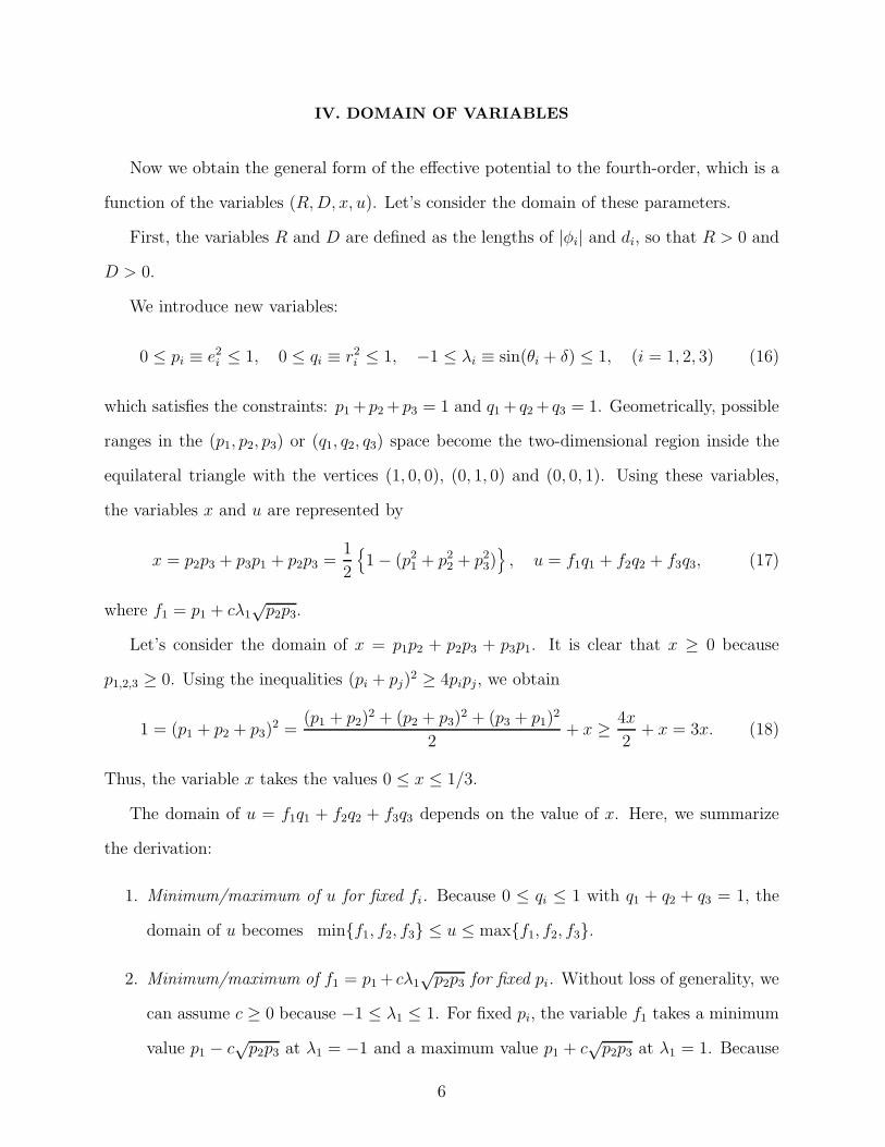
IV. DOMAIN OF VARIABLES

Now we obtain the general form of the effective potential to the fourth-order, which is a

function of the variables (R,D, x, u). Let’s consider the domain of these parameters.

First, the variables R and D are defined as the lengths of |φi| and di, so that R > 0 and

D > 0.

We introduce new variables:

0 ≤ pi ≡ e2i ≤ 1, 0 ≤ qi ≡ r2i ≤ 1, −1 ≤ λi ≡ sin(θi + δ) ≤ 1, (i = 1, 2, 3) (16)

which satisfies the constraints: p1+ p2+ p3 = 1 and q1+ q2+ q3 = 1. Geometrically, possible

ranges in the (p1, p2, p3) or (q1, q2, q3) space become the two-dimensional region inside the

equilateral triangle with the vertices (1, 0, 0), (0, 1, 0) and (0, 0, 1). Using these variables,

the variables x and u are represented by

x = p2p3 + p3p1 + p2p3 =1

2

{

1− (p21 + p22 + p23)}

, u = f1q1 + f2q2 + f3q3, (17)

where f1 = p1 + cλ1√p2p3.

Let’s consider the domain of x = p1p2 + p2p3 + p3p1. It is clear that x ≥ 0 because

p1,2,3 ≥ 0. Using the inequalities (pi + pj)2 ≥ 4pipj, we obtain

1 = (p1 + p2 + p3)2 =

(p1 + p2)2 + (p2 + p3)

2 + (p3 + p1)2

2+ x ≥ 4x

2+ x = 3x. (18)

Thus, the variable x takes the values 0 ≤ x ≤ 1/3.

The domain of u = f1q1 + f2q2 + f3q3 depends on the value of x. Here, we summarize

the derivation:

1. Minimum/maximum of u for fixed fi. Because 0 ≤ qi ≤ 1 with q1 + q2 + q3 = 1, the

domain of u becomes min{f1, f2, f3} ≤ u ≤ max{f1, f2, f3}.

2. Minimum/maximum of f1 = p1+ cλ1√p2p3 for fixed pi. Without loss of generality, we

can assume c ≥ 0 because −1 ≤ λ1 ≤ 1. For fixed pi, the variable f1 takes a minimum

value p1 − c√p2p3 at λ1 = −1 and a maximum value p1 + c

√p2p3 at λ1 = 1. Because

6

fi are defined symmetrically for the index (i = 1, 2, 3), similar results are obtained for

f2 and f3.

3. Range of u for fixed pi. Combining the above results 1. and 2. , we obtain the possible

range of u for fixed pi: f−1 ≤ u ≤ f+

1 , where

f−1 = p1 − c

√p2p3, f+

1 = p1 + c√p2p3. (19)

4. Finally the domain of u for the fixed value of x is obtained by min{

f−1 , f

−2 , f

−3

}

≤ u ≤

max{

f+1 , f

+2 , f

+3

}

where min and max are for 0 ≤ pi ≤ 1 with p1 + p2 + p3 = 1.

Thus, the evaluation of the domain of u has been reduced to those of min(f−) and max(f+),

which are somewhat complicated because they depend not only on the coefficient c but also

on the variable x. The calculations for them are given in appendix B, and we show only the

final results for the domain of (x, u) below.

The results are given for (0 ≤ c ≤ 2) and (2 ≤ c), which are respectively shown in

figure 1(a) and (b). These figures show upper and lower bounds of u for fixed x.

a : 0 ≤ c ≤ 2

Upper bound of u :2− c

3

√1− 3x+

1 + c

3(20)

Lower bound of u :

−c√x (0 ≤ x ≤ 1

4)

−2+c3

√1− 3x+ 1−c

3(14≤ x ≤ 1

3)

(21)

The segment AB in figure 1(a) corresponds to eq. (20), and OC and CD to two equations

in (21).

b : 2 ≤ c

Upper bound of u :

− c−23

√1− 3x+ 1+c

3

(

0 ≤ x ≤ (2c−1)2

4(c2−c+1)2

)

c√x

(

(2c−1)2

4(c2−c+1)2≤ x ≤ 1

4

)

c−23

√1− 3x+ 1+c

3(14≤ x ≤ 1

3)

(22)

Lower bound of u :

−c√x (0 ≤ x ≤ 1

4)

−2+c3

√1− 3x+ 1−c

3(14≤ x ≤ 1

3)

(23)

7

The segments AE,EF and FB in figure 1(b) correspond to three divisions in eq. (22), and

OC and CD to two equations in (23).

V. STABILITY CONDITION

For the system with the effective potential Veff to be physically meaningful, it should be

positive definite when the variables R or D take infinitely large value. (If not, any states

with finite R and D become unstable.)

This stability (positive definite) condition gives constraints on the parameters gi and hi

in eq. (12) and we derive them in this section. First, we consider special cases:

1. When D = 0 and R → ∞, eq. (12) become Veff ∼ g′RR4

2. When R = x = 0 and D → ∞, we obtain Veff ∼ g′DD4.

From the positive definineness of Veff in these limits, the first two constraints can be obtained:

g′D ≥ 0, g′R ≥ 0. (24)

Hereafter, we consider the cases of g′D > 0 and g′R > 0 only. (We can treat the cases that

g′D = 0 or g′R = 0 with taking the limit of those in g′D > 0 and g′R > 0.)

We replace the variables R and D by the scaled ones: R → R/(g′R)1

4 and D → D/(g′D)1

4 ,

then eq. (12) becomes

Veff = −GR2 +R4 − FD2 + (1 + F ′x)D4 + 2(H +H ′u)R2D2, (25)

where scaled parameters are defined by

G = − gR√

g′R, F = − gD

√

g′D, F ′ = −hD

g′D, H =

g′′D

2√

g′Dg′R

, H ′ =h′′D

2√

g′Dg′R

. (26)

For large values of R2 and D2, eq. (25) behaves as a linear quadratic form of them for

any fixed values of (x, u): Veff ∼ R4 + (1 + F ′x)D4 + 2(H + H ′u)R2D2. The Sylvester’s

theorem should give the positive definite condition for it [12]:

8

a) 1 + F ′x− (H +H ′u)2 ≥ 0

or

b) 1 + F ′x ≥ 0 and H + H′u ≥ 0, (27)

for any values of (x, u), the domain of which have been shown in figure 1(a) and (b). The

second condition b) in eq. (27) should be required because R2, D2 ≥ 0.

The condition (27) gives constraints for the possible values of parameters F ′, H and H ′,

which can be obtained analytically. We sketch the derivation of them in Appendix C, and

only show the results here.

Stability conditions in (H,F ′) space for fixed c and H ′ are classified at first into two

types for (0 ≤ c ≤ 2) and (2 ≤ c), and then into four types by the values of H ′ in each of

the first two (which correspond to four subscripts I∼IV in figure 2 and figure 3), which are

shown in figure 2(a)∼(d) for 0 ≤ c ≤ 2, in figure 3(a)∼(d) for 2 ≤ c. In the following lists,

we obtain complete stability conditions for the coefficients F ′, H , H ′ and c in eq. (25).

A. 0 ≤ c ≤ 2 case

a : H ′ ≤ − 32−c

(figure 2(a))

F ′ ≥ −3, (−H ′ − 1 ≤ H) (28)

This critical point (−H ′ − 1,−3) corresponds to the point A in figure 2(a).

b : − 32−c

≤ H ′ ≤ 0 (figure 2(b))

F ′ ≥ k(c),(

−H ′ − 1 ≤ H ≤ −1 + c

3H ′)

AB (29)

F ′ ≥ −3,(

−1 + c

3H ′ ≤ H

)

B∞ (30)

where k(c) = 3

2

[

(H +H ′)(

H + 2c−1

3H ′)

− 1−√

{(H +H ′)2 − 1}{

(

H + 2c−1

3H ′

)2 − 1}

]

.

c: 0 ≤ H ′ ≤ 32+c

(figure 2(c))

9

F ′ ≥ (cH′)2

1−H2 , (−1 ≤ H ≤ H1) ∞A (31)

F ′ ≥ (2H − cH ′)2 − 4, (H1 ≤ H ≤ H2(c)) AB (32)

F ′ ≥ k(−c),(

H2(c) ≤ H ≤ c− 1

3H ′)

BC (33)

F ′ ≥ − 3,(

c− 1

3H ′ ≤ H

)

C∞ (34)

where H1 ≡ cH′−√16+c2H′2

4, H2(c) =

(3c+2)H′−√

16+(c+2)2H′2

4.

d: 32+c

≤ H ′ (figure 2(d))

F ′ ≥ (cH ′)2

1−H2, (−1 ≤ H ≤ H1) ∞A (35)

F ′ ≥ (2H − cH ′)2 − 4,

(

H1 ≤ H ≤ cH ′ − 1

2

)

AB (36)

F ′ ≥ −3,

(

cH ′ − 1

2≤ H

)

B∞ (37)

B. 2 ≤ c case

a: H ′ ≤ − 3c−2

(figure 3(a))

F ′ ≥ (2H + cH ′)2 − 4,

(

−H ′ − 1 ≤ H ≤ −1 + cH ′

2

)

AB (38)

F ′ ≥ −3,

(

−1 + cH ′

2≤ H

)

B∞ (39)

b: − 3c−2

≤ H ′ ≤ 0 (figure 3(b))

F ′ ≥ (2H + cH ′)2 − 4, (−H ′ − 1 ≤ H ≤ H2(−c)) AB (40)

F ′ ≥ k(c),(

H2(−c) ≤ H ≤ −1 + c

3H ′)

BC (41)

F ′ ≥ −3,(

−1 + c

3H ′ ≤ H

)

C∞ (42)

c: 0 ≤ H ′ ≤ 32+c

(figure 3(c))

10

F ′ ≥ (cH ′)2

1−H2, (−1 ≤ H ≤ H1) ∞A (43)

F ′ ≥ (2H − cH ′)2 − 4, (H1 ≤ H ≤ H2(c)) AB (44)

F ′ ≥ k(−c),(

H2(c) ≤ H ≤ c− 1

3H ′)

BC (45)

F ′ ≥ −3,(

c− 1

3H ′ ≤ H

)

C∞ (46)

d: 32+c

≤ H ′ (figure 3(d))

F ′ ≥ (cH ′)2

1−H2, (−1 ≤ H ≤ H1) ∞A (47)

F ′ ≥ (2H − cH ′)2 − 4,

(

H1 ≤ H ≤ cH ′ − 1

2

)

AB (48)

F ′ ≥ −3,

(

cH ′ − 1

2≤ H

)

B∞ (49)

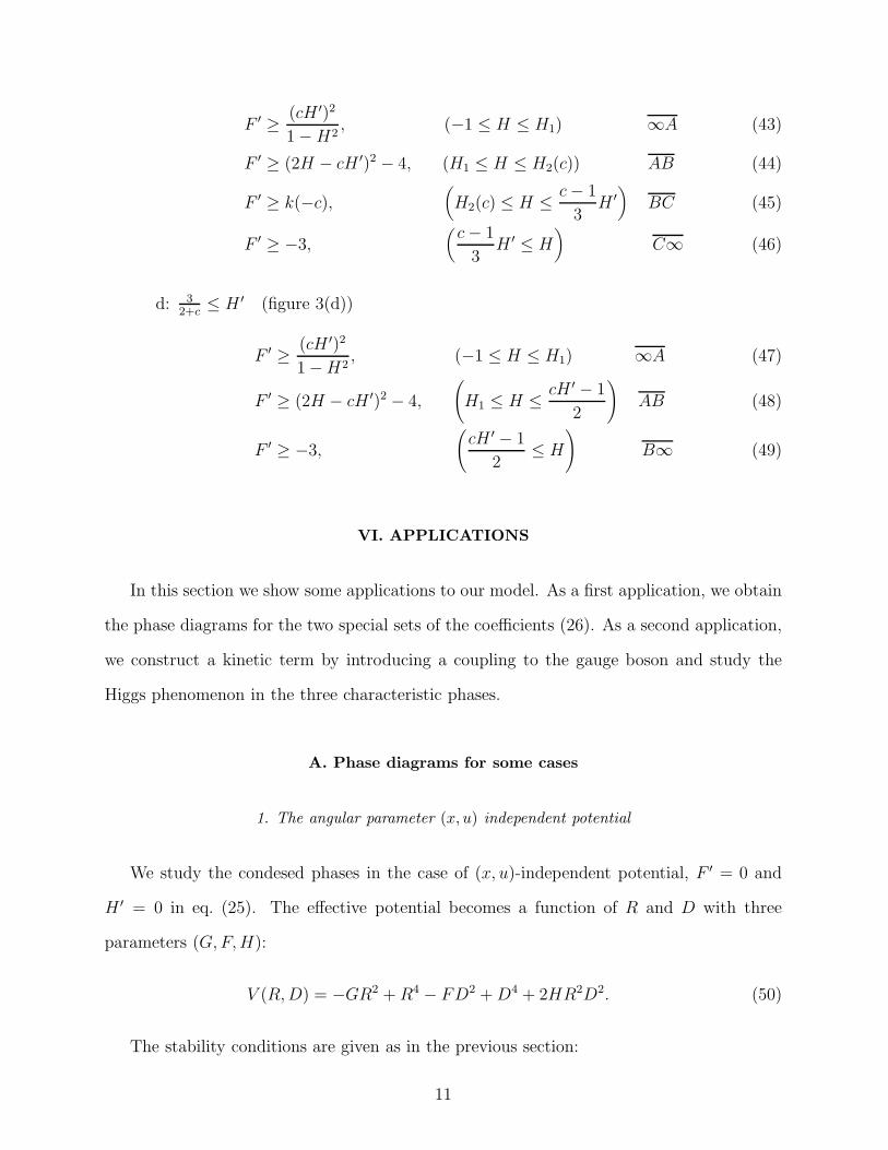
VI. APPLICATIONS

In this section we show some applications to our model. As a first application, we obtain

the phase diagrams for the two special sets of the coefficients (26). As a second application,

we construct a kinetic term by introducing a coupling to the gauge boson and study the

Higgs phenomenon in the three characteristic phases.

A. Phase diagrams for some cases

1. The angular parameter (x, u) independent potential

We study the condesed phases in the case of (x, u)-independent potential, F ′ = 0 and

H ′ = 0 in eq. (25). The effective potential becomes a function of R and D with three

parameters (G,F,H):

V (R,D) = −GR2 +R4 − FD2 +D4 + 2HR2D2. (50)

The stability conditions are given as in the previous section:

11

1−H2 ≥ 0 or H ≥ 0. (51)

Four kinds of condensesd phase (as extremum points of the effective potential) are ob-

tained: 1) R0 = D0 = 0 , 2) R0 6= 0, D0 = 0 , 3) R0 = 0, D0 6= 0 , 4) R0 6= 0,

D0 6= 0 corresponding to eqs. (4)-(7), and the parameter regions for each phase are shown

in Table 1 with the conditions (51). Referring to Table 1, the phase diagram on (F, G)

space for fixed H is obtained in figure 4 by comparing V (R0, D0) in the ranges where more

than two kinds of extrema exist. At H=−1, the mixed phase emerges above the line AB

(G=−F ) in figure 4(a), and as H increases to 1 the two branches of this line merges into

the line OA (G = F ) in figure 4(c). When H exceeds 1 the mixed phase vanishes.

2. The potential for the symmetric phase

Next we study the case in which only the symmetric 6 phase emerges, i.e.,

gR=g′R=g′′D=h′′D=0 in eq. (12). In this case the effective potentail is given by

V (x,D) = gDD2 + (g′D − hDx)D

4. (52)

From 0 ≤ x ≤ 13, we obtained the stability condition by

hD ≤ 3 g′D, g′D ≥ 0. (53)

This condition coincides with the previous results in F≥−3 and H ′=H= 0, e.g., in eqs. (29)

and (30). From eq. (52) the four kinds of condensed phase are obtained: 1) D0=0 , x=0, 2)

D0 6=0, x=0, 3) D0 6=0, 4) D0 6=0, x=13. The parameter regions and the form of the order

parameter S0 in eq. (9) for each phase are given in Table 2. The phase diagram in (F , G)

space for gD≥0 is shown in figure 5.

It is noticed that the linear dependence of the effective potential (52) on x is the reason

why the phase characterized by, e.g., S0=(d1, d2, 0) does not emerge.

12

B. Higgs phenomenon

Higgs phenomenon is the one where gauge bosons acquire finite effective masses in the

broken-symmetry phase. In the minimal coupling scheme, the gauge boson fields Aaµ are

introduced through the kinetic terms of the order parameter. To the second-order, it is

given by

Kkinetic = −kATr(DµA)∗DµA + kSTr(DµS)

∗DµS, (54)

where the coefficients kA and kS are positive constants. The covariant derivative Dµ in

eq. (54) is defined by

DµΨ ≡ ∂µΨ− igλa

2Aa

µΨ− igΨtλa

2Aa

µ, (55)

where g and λa=1∼8 are the gauge coupling constant and the Gell-Mann matrices [14].

The effective masses of the gauge bosons are obtained from the second-order terms of

the gauge boson fields in the kinetic terms (54).

1. The 3∗ condensed phase

In the case of the 3∗ condensed phase we consider an order parameter

Ψ0 =

0 −a 0

a 0 0

0 0 0

, (56)

where a is a real constant. Note that this form is general enough since other forms of the

3∗ phase is obtained by a simple transformation to Ψ0 as in eq. (8). In this phase SUc(3)

symmetry breaks into SU(2).

By substituting Ψ0 into eq. (54) the mass terms are obtained: m2vTrv

†v and m2φTrφ

2

where mv≡√2kA|a|g, mφ≡

√

43kA|a|g, v=1

2(λ4 + iλ5)(A

4µ + iA5

µ) +12(λ6 + iλ7)(A

6µ + iA7

µ) and

φ=λ8A8µ. The gauge fields v and φ are different multiplets of the residual symmetry SU(2).

13

This phase is the one which is featured in most microscopic models. Using the values of

the gauge coupling constant g and the gap |a| caluculated in models [4], the effective masses

are estimated: mv=√

32mφ ∼ 100 MeV.

2. The 6 condensed phase

We select an order parameter proportional to the identity matrix which is discussed in

the previous application, see Table 2 :

Ψ0 =

a 0 0

0 a 0

0 0 a

. (57)

In this phase SU(3) symmetry breaks into SO(3). Since the gauge boson field Aµ(≡λaAaµ) is

transformed as direct products of two triplets under the SO(3) group, they are decomposed

into the direct sum of triplet (anti-symmetric part) and quintet (symmetric part):

Aµ = V3 + T5, (V3 ≡∑

a=2,5,7

λaAaµ), (T5 ≡

∑

a=1,3,4,6,8

λaAaµ). (58)

Since T5 is assigned to the generators of the broken symmetry SU(3)/SO(3), the mass term

is accompanied with the quintet term: m2TTr(T5)

2, where mT≡√4kS|a|g.

3. The Mixed condensed phase

We study a special case for the mixed phase characterized by the order parameter:

Ψ0 =

0 0 0

0 0 0

a 0 0

. (59)

In this phase SU(3) symmetry breaks into U(1) which is generated by H(t)=ei(λ3+√3λ8)t.

Since in this case the multiplets of the gauge field are not trivial, we investigate a dependence

of the gauge field Aµ on the infinitesimal transformation of H(t).

14

(HAµH†)kl ∼ (Aµ)kl + (P )kl(Aµ)kl, P = i

0 1 2

−1 0 1

−2 −1 0

t (60)

Noticing that (λ3 +√3λ8) and (λ3 − 1√

3λ8) are orthogonal each other, the gauge field are

decomposed into the multiplets:

Aµ =

0 ξ η

ξ∗ 0 ζ

η∗ ζ∗ 0

+ (λ3 −1√3λ8)ϕ+ (λ3 +

√3λ8)ϕ

′, (61)

ξ ≡ A1µ − iA2

µ, η ≡ A4µ − iA5

µ, ζ ≡ A6µ − iA7

µ

ϕ ≡ (3A3µ −

√3A8

µ)/4, ϕ′ ≡ (A3µ +

√3A8

µ)/4.

The mass terms are summerized as follows:

m2ξ ξ

∗ξ =1

2(kA + kS)|a|2g2ξ∗ξ, m2

ηη∗η = 2kS|a|2g2η∗η

m2ζζ

∗ζ =1

2(kA + kS)|a|2g2ζ∗ζ, mϕϕ

2 =16

18(kA + kS)|a|2g2ϕ2. (62)

In the same way more complicated cases can also be studied.

VII. SUMMARY

We have derived the general form of the Color-SU(3)-Ginzburg-Landau Effective Poten-

tial for the order parameter with 3×3 symmetry to the fourth-order and determined the

range of coefficients which stabilizes the vacuum of the system. Corresponding to the irre-

ducible components of the order parameter 3×3=3∗+6, we found four kinds of phases: non

condensed phase, anti-symmetric (3∗) phase, symmetric (6) phase and mixed (3∗+6) phase.

As applications, we obtained the phase diagrams in the two special cases and studied

the Higgs phenomenon in some characteristic phases by gauging this model.

The full classification of the broken vacuum are analytically possible including the angular

parameter x and u, and will be discussed in different paper.

15

APPENDIX A: NORMAL COORDINATE DECOMPOSITION

In this appendix, we show the decomposition of the 3-by-3 symmetric matrix S = tS in

eq. (9). The proof is a variation of that used in the group representation theory [13], the

SU(3)-chiral nonlinear sigma model [14] and the Kobayashi-Maskawa theory of quark mass

matrix [15].

We take the subsidery hermite matrixH = S∗S = S†S. Its eigenvalue λi and eigenvectors

ei are obtained from the eigenequation: Hei = λiei (i = 1, 2, 3).

In this appendix, we consider only the case of no degeneracy: λi 6= λj (i 6= j). (The

extension to degenerate cases should be made by analytic continuation. )

Because of the hermiticity of H , the eigenvectors ei can be taken to be orthogonal unit

vectors (†eiej = δij), and the eigenvalues λi take real positive values. (because of H = S†S).

In matrix form, the eigenequation becomes

U †HU = L ≡

λ1 0 0

0 λ2 0

0 0 λ3

, (A1)

where U = (e1, e2, e3) ∈ SU(3).

The eigenvector ei satisfies

H∗Sei = SS∗Sei = SHei = λiSei. (A2)

so that we obtain Sei = αie∗i (because H∗e∗i = λie

∗i ). αi ≡ |αi|eiθi are complex numbers. In

matrix form, it becomes

tUSU = Z ≡

α1 0 0

0 α2 0

0 0 α3

. (A3)

The polar decomposition of Z becomes

A = ReiT =

|α1| 0 0

0 |α2| 0

0 0 |α3|

eiθ1 0 0

0 eiθ2 0

0 0 eiθ3

, T =

θ1 0 0

0 θ2 0

0 0 θ3

. (A4)

16

Because of λiei = Hei = S∗Sei = αiS∗e∗i = αi(Sei) = |αi|2ei, we obtain λi = |α|i and

also R =√L. The polar decomposition of A becomes A =

√LeiT .

Because the angular part T is diagonal, it can be expanded by the 3-by-3 unit matrix

I and the diagonal Gell-Mann matrices λ3,8: T = θI + φ3λ3 + φ8λ8. If we define K =

ei

2(φ3λ3+φ8λ8), then we obtain eiT = KeiθIK. Using the first equation in (A4), the matrix S

becomes

S = U∗ZU = U∗√LeiTU † = eiθU∗K

√LKU † = eiθG

√L tG, (A5)

where G ≡ U∗K and tG = tKU † = KU †. This is just the decomposition of S in eq. (8) with

S0 =√L.

If we define the matrix A0 by A = GA0tG, then A0 also becomes antisymmetric and is

generally represented as the first equation in eq. (9).

APPENDIX B: MAXIMUM AND MINIMUM OF f

Instead of pi with p1 + p2 + p3 = 1, we take independent variables (s, t):

s =1√2(−p1 + p2), t = −

√

3

2

(

p1 + p2 −2

3

)

. (B1)

The possible range of (s, t) is determined from the condition: 0 ≤ pi ≤ 1 and p1+p2+p3 = 1.

Using (B1), it is found to be the inside of the equilateral triangle with vertices (0,√

2/3)

and (±1/√2,−1/

√6) in the (s, t) plane. Since the function f(s, t) is an even function of s,

f(s, t) = f(−s, t), we may consider a half (s ≥ 0) of the triangular region (figure 6) to find

its maximum/minimum.

For a fixed value of x, a trajectory of x = p2p3+p3p1+p1p2 = −(s2+ t2)/2+1/3 in (s, t)-

plane become a circle with the center (0, 0) and the radius√

(2/3)− 2x (figure 6). From

the aspect of intersections between the circle and the triangular region, two cases should be

discriminated:

17

1. When 0 ≤ x < 1/4, the circle intersects with three sides of the triangle (figure 6(a)),

and the two separate arcs (B0B1 and B2B3 in figure 6(a)) are included in the half

triangular region.

2. When 1/4 ≤ x ≤ 1/3, the whole circle is included in the triangular region (figure 6(b)).

The intersections with the s-axis (t = 0) are denoted by B0 and B4.

The (s, t)-coordinates of the above four points B0∼4 are given by

B0 =

0,

√

2

3− 2x

, B1 =

(

1−√1− 4x

2√2

,1 + 3

√1− 4x

2√6

)

, (B2)

B2 =

(

1 +√1− 4x

2√2

,1− 3

√1− 4x

2√6

)

, B3 =

√

1− 4x

2,− 1√

6

, (B3)

B4 =

0,−√

2

3− 2x

. (B4)

Let’s consider the maximum value of f+3 for fixed values of c and x. Using s =

√6− 9t2 − 18x/3 and (B4), f+

3 in eq. (19) becomes

f+3 (t) =

1

3

[√6t + 1 + c

√

6t2 −√6t+ 9x− 2

]

, (B5)

where we take t as an independent variable and (x, c) as any fixed parameters. Solving

the equation [f+3 (t)]

′ = 0, we obtain one local extremum at BM = (√

6− 9t2M − 18x/3, tM)

where

tM =1

2√6

1− 3

√

(4x− 1)(c2 − 1)

1− c2

. (B6)

for some values of (x, c). The parameter range where the extremum of f+3 exists (at BM) can

be read off from the condition that tM in (B6) should take a real value: i.e., (4x−1)(c2−1) ≥

0. Solving this inequality, we obtain two separated regions: a) c ≤ 1 & x ≤ 1/4 and b) c ≥ 1

& x ≥ 1/4 (Shaded regions in figure 7) where the function f+3 has an extremum. Judging

from the signature of [f+3 ]

′′(tM), we can find that f+3 (tM) is a local maximum in region a)

and minimum in region b). For tM have to be in the permissible region shown in figures 6(a)

and (b), we obtain further condition:

18

1. When x ≤ 1/4 and c ≤ 1, tM have to be on the arc B2B3 (figure 6(a)). Thus, we

obtain x ≥ c2/4 (OD in figure 7).

2. When x > 1/4, tM have to be on the half circle B0B4 (figure 6(b)). Thus, we obtain

c ≤ 2 or x ≤ c(5c− 4)/[4(2c− 1)2] (AB in figure 7),

Summarizing the above discussions about the aspects of extrema of f+3 , we can classify the

five regions in the (c, x)-plane (figure 7).

Let’s analyze maximum points in each regions. Candidates of the absolute maximum

point of f 3+ are the end points B0∼4 where

f 3+(B0) =

1+c3

+ 2−c3

√1− 3x, f 3

+(B1) =1

2+

1

2

√1− 4x,

f 3+(B2) =

12− 1

2

√1− 4x, f 3

+(B3) = c√x,

f 3+(B4) =

1+c3

− 2−c3

√1− 3x, (B7)

or the local maximum at M (if exist):

f 3+(BM) =

1

2− 1

2

√

(c2 − 1)(4x− 1). (B8)

Comparing f 3+(Bi) in eqs. (B7) and (B8), we can find maximum points in each region in

figure 7:

1. The maximum is at B0 in regions 1, 2, a part of 3 (c ≤ 2 or x ≤ (2c−1)2/[4(1−c+c2)2]

EF in figure 8 ), and a part of 4 (c ≤ 2).

2. The maximum is at B3 in a remaining part of region 3.

3. The maximum is at B4 in region 5 and a remaining part of 4.

The results are summarized in figure 8.

In a similar way, the minimum value of f−3 (t) can be calculated:

f−3 (t) =

c√x (0 ≤ x < 1/4)

1−c3

− 2+c9

√1− 3x (1/4 ≤ x ≤ 1/3)

(B9)

19

APPENDIX C: DERIVATION OF STABILITY CONDITIONS

In this appendix, we sketche the derivation of the stability condition: a parameter range

of (F ′, H,H ′) that satisfies (27).

Instead of (x, u), we take new variables (X,U) defined by

X ≡ 1 + F ′x, U ≡ H +H ′u. (C1)

Using them, the conditions in (27) become simple:

a) X ≥ U2, or b) X ≥ 0 and U ≥ 0. (C2)

In the (X,U)-plane, the range that satisfies these conditions is represented by the hatched

area in figure 9. We denote it by the region Σ.

The possible range of variables (X,U), which is translated from the one of (x, u) (given

in figure 1), depends on parameters (F ′, H ′, c) and we denote it by Λ(F ′, H ′, c). In figure 9,

as an example, we show the Λ(F ′, H ′, c) as the cross-hatched region for some values of

(F ′, H ′, c) that satisfies F ′ ≥ 0, H ′ ≥ 0 and c ≥ 2. In (X,U)-plane, the stability condition

(27) become equivalent with the geometrical condition:

Λ(F ′, H ′, c) ⊂ Σ. (C3)

The boundary of Λ(F ′, H ′, c) and Σ are patchworks of line or parabolic segments, so that

the condition (C3) can be solved algebraically.

As an example, let’s consider the case that c ≤ 2, F ′ ≥ 0 and H ′ ≥ 0 (figure 9). In this

case, eq. (C3) can be attributed into whether the boundary segment ∞GO for Σ intersects

that of Λ, AB, or not. Both segments, ∞GO and AB, have parabolic shapes represented

by X = U2 (∞GO) and X = [F ′/(cH ′)2](U − H)2 + 1 (AB). It can be judged from the

condition that the edge points, A = (1, H) and B = (F′

4+ 1, H − cH′

2), are included in Σ; it

gives two necessary conditions for parameters:

−1 ≤ H,

(

H − cH ′

2

)2

≤ F ′

4+ 1. (C4)

20

In case that F ′/(cH ′)2 ≤ 1, the slope of ∞GO is more gradual than that of AB, and eqs.

(C4) are sufficient condition. However, in the case that F ′/(cH ′)2 ≥ 1, an extra condition

should be added in order that two parabolic segments have no intersections:

(cH ′)2 + F ′(H2 − 1) < 0. (C5)

Eqs. (C4) and (C5) give the necessary and sufficient stability condition in that case:

F ′ ≥ (cH ′)2

1−H2, F ′ ≥ (2H − cH ′)2 − 4, −1 ≤ H, (C6)

which is shown as the hatched region in figure 2.

Other cases can be treated in a similar way.

21

REFERENCES

[1] Barrois F 1977 Nucl. Phys. B129 390

[2] Bailin D and Love A 1984 Phys. Rep. 107 325

[3] Iwasaki M 1996 Prog. Theor. Phys. 96 1043

[4] Rapp R, Schafer T, Shuryak E and Velkovsky M 1998 Phys. Rev. Lett. 81 53

Alford M, Rajagopal K and Wilczek F 1998 Phys. Lett. B422 247.

[5] Son D T 1999 Phys. Rev. D59 094019

Schafer T and Wilczek F 1998 Phys. Lett. B450 325

Hsu S and Schwetz M 2000 Nucl. Phys. B572 211

[6] Schafer T and Wilczek F 1999 Phys. Rev. D60 114033

Brown W E, Liu J T and Ren H 2000 Phys. Rev. D62 054016

Pisarski R D and Rischke D H 2000 Phys. Rev. D61 074017

[7] Alford M, Rajagopal K and Wilczek F 1999 Nucl. Phys. B537 443

Shovkovy I A and Wijewardhana L C R 1999 Phys. Lett. B470 189

[8] Casalbuoni R and Gatto R 1999 Phys. Lett. B464 111

Rho M, Wirzba A and Zahed I 2000 Phys. Lett. B473 126

[9] Berges J and Rajagopal K 1999 Nucl. Phys. B538 215

Miransky V A, Shovkovy I A and Wijewardhana L C R 1999 Phys. Lett. B468 270

[10] For example, Tilley D R and Tilley J 1986 “Superfluidity and Superconductivity”, 2nd

ed. Adam Hilger Ltd

[11] Iida K and Baym G 2001 Phys. Rev. D63 074018

Giannakis I and Ren H 2002 Phys.Rev. D65 054017

Sedrakian D M, Blaschke D, Shahabasyan K M and Voskresensky D N 2001 Astrofiz.

44 443

22

[12] Gradshteyn I S and Ryzhik I M 1990 “Tables of Integral, Series, and Products”, 5th ed.

(translated from Russian by Scripta Technica Inc.) San Diego, Academic Press

[13] Murnaghan F D 1938 “The Theory of Group Representations” Baltimore, The John

Hopkins Press

[14] Lee B 1972 “Chiral Dynamics” New York, Gordon and Breach Sci. Pub.

[15] Kobayashi M and Maskawa T 1973 Prog. Theor. Phys. 49 652

23

figure 1. Range of variables x and u. a) for 0 ≤ c ≤ 2, b) for 2 ≤ c. Details are given in

the text.

figure 2. Stability region in (H,F ′) space for (0 ≤ c ≤ 2) (the shaded area). figure 2(a) is

for H ′ ≤ − 32−c

, (b) for − 32−c

≤ H ′ ≤ 0, (c) for 0 ≤ H ′ ≤ 32+c

and (d) for 32+c

≤ H ′.

figure 3. Stability region in (H,F ′) space for (2 ≤ c). figure 3(a) is for H ′ ≤ − 3c−2

, (b)

for − 3c−2

≤ H ′ ≤ 0, (c) for 0 ≤ H ′ ≤ 32+c

and (d) for 32+c

≤ H ′.

figure 4. (a) The phase diagram for the effective potential (50) in (F,G) space when H=−1.

AB : G=−F . The regions with vertical stripes, with horizontal stripes and with cross

hatch show 3∗, 6 and the Mixed condensed phases. The remaining part (G ≤ 0 and

F ≤ 0) shows the Non condensed phase. (b) The same, but H=1/2. OA : G=2F .

OB : G=F/2. (c) The same, but H=1. OA : G=F .

figure 5. The phase diagram for the effective potential (52) in (g′D, hD) space when gD<0.

AB : hD=3g′D. The regions I and II corresponds to the phases 2) and 4) in Table 2,

but the region just on the line hD=0 (g′D>0) corresponds to the phase 3).

figure 6. Range of variables s and t is shown as inside of the half triangle ACD. Trajectories

of (s, t) for fixed x are given for 0 ≤ x ≤ 14by two separate arcs B0B1 and B2B3 in

(a) and for 14≤ x ≤ 1

3by a half circle B0B4 in (b).

figure 7. The five regions in the (c, x)-plane according to the aspects of tM . tM is defined

in the shaded regions. In addition, in the region 1 and 4 tM exists on the arc B2B3

(figure 6(a)), and on the half circle B0B4 (figure 6(b)).

figure 8. The three regions in the (c, x)-plane separated by the maximum values of f 3+,

which are f 3+(B0) , f

3+(B3) and f 3

+(B4) in the region I, II and III.

figure 9. An illustration for the stability condition Λ(F ′, H ′, c) ⊂ Σ in the case c ≤ 2, F ′

≥ 0 and H ′ ≥ 0.

24

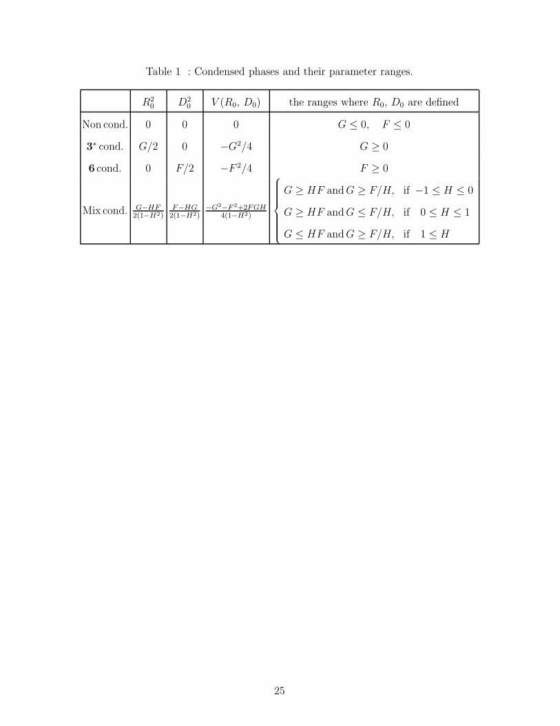
Table 1 : Condensed phases and their parameter ranges.

R20 D2

0 V (R0, D0) the ranges where R0, D0 are defined

Non cond. 0 0 0 G ≤ 0, F ≤ 0

3∗ cond. G/2 0 −G2/4 G ≥ 0

6 cond. 0 F/2 −F 2/4 F ≥ 0

Mix cond. G−HF2(1−H2)

F−HG2(1−H2)

−G2−F 2+2FGH4(1−H2)

G ≥ HF andG ≥ F/H, if −1 ≤ H ≤ 0

G ≥ HF andG ≤ F/H, if 0 ≤ H ≤ 1

G ≤ HF andG ≥ F/H, if 1 ≤ H

25

Table 2 : Forms of the order parameter and their parameter ranges

(D20, x) S0 = (d1, d2, d3) the parameter region

1) (0, 0) d1 = d2 = d3 = 0 gD ≥ 0

2) (− gD2g′

D

, 0) di 6= 0, dj 6=i = 0 gD < 0, hD < 0

3) (− gD2g′

D

, x) d21 + d22 + d23 = D20 gD < 0, hD = 0

4) (− gD2(g′

D−hD/3)

, 13) d1 = d2 = d3 6= 0 gD < 0, 0 < hD ≤ 3g′D

26

x

x

jkn

m ll

k j

m

x

c

x

c