Embed Size (px)
Citation preview

HAL Id: hal-00762602https://hal.archives-ouvertes.fr/hal-00762602
Submitted on 7 Dec 2012
HAL is a multi-disciplinary open accessarchive for the deposit and dissemination of sci-entific research documents, whether they are pub-lished or not. The documents may come fromteaching and research institutions in France orabroad, or from public or private research centers.
L’archive ouverte pluridisciplinaire HAL, estdestinée au dépôt et à la diffusion de documentsscientifiques de niveau recherche, publiés ou non,émanant des établissements d’enseignement et derecherche français ou étrangers, des laboratoirespublics ou privés.
Dependability Evaluation of an Air Traffic ControlComputing System
Nicolae Fota, Mohamed Kaâniche, Karama Kanoun
To cite this version:Nicolae Fota, Mohamed Kaâniche, Karama Kanoun. Dependability Evaluation of an Air TrafficControl Computing System. Performance Evaluation, Elsevier, 1999, 35 (3-4), pp.253-273. <hal-00762602>

Dependability Evaluation
of an Air Traffic Control Computing System
Nicolae Fota* Mohamed Kaâniche
!
and Karama Kanoun!
!
LAAS-CNRS *SOFREAVIA
7, Av. du Colonel Roche 3 Carrefour de Weiden
31077 Toulouse Cedex 4 —France 92441 Issy les Moulineaux—France
{kaaniche;kanoun}@laas.fr [email protected]
Author Contact: Mohamed Kaâniche
Abstract*
As air traffic over France is growing rapidly, the existing Air Traffic Control (ATC) system has to
evolve to satisfy the increasing demand. The selection of the new automated computing system (denoted
CAUTRA) is based, among other things, on dependability evaluation. This paper is devoted to the
dependability evaluation of the CAUTRA, however, emphasis is put on a subset: the Regional Control
Center (RCC). Starting from the analysis of the impact of CAUTRA failures on air traffic safety, five
levels of service degradation are defined for the global system grading the effects of these failures on
the service delivered to the controllers to ensure traffic safety. The RCC failure modes leading to these
degradation levels are then defined and evaluated using stochastic Petri nets. The modeling approach
consists in modeling the system as a set of modules interconnected via coupling mechanisms. The
system model is constructed in several steps according to an incremental approach. Each step
integrates the failure and recovery assumptions of an additional component and updates the model of
the previous step by accounting for the impact of the new component on the behavior of those already
included in the model. The application of this approach to the CAUTRA allowed us to analyze several
configurations of the CAUTRA architecture and to identify improvement areas to minimize the impact
of CAUTRA failures on air traffic safety.
* Nicolae Fota was at LAAS-CNRS when this work was performed.

2
Key words: Dependability modeling, stochastic Petri nets, Markov chains, air traffic control, air traffic
safety, safety analysis
1. Introduction
The French Air Traffic Control (ATC) is based on an automated system (the CAUTRA),
implemented on a distributed fault-tolerant computing system composed of five Regional en-route air
traffic Control Centers (RCC) and one Centralized Operating Center (COC), connected through a
dedicated Telecommunication Network (TN). The same computer architecture is implemented in each
RCC. The CAUTRA design has been in a continuous evolution during the last few years in order to
face the growth of air traffic volume, to improve the dependability of the CAUTRA and to include
additional functionality to the controller. The definition of the new CAUTRA architecture is supported
by quantitative evaluation techniques. In this context, our work focuses on the analysis and evaluation
of the impact of CAUTRA failures on the service delivered to the controller to ensure air traffic safety.
The analysis and evaluation of this impact has been performed in three successive phases. The first
one, aimed at a preliminary Failure Modes Effects and Criticality Analysis of the CAUTRA, led us to
define five levels of ATC service degradation and to identify the main subsystems providing vital
services for air traffic safety. The second phase focused on the dependability modeling and evaluation
of each of these subsystems. The third phase was devoted to the combination of the dependability
measures evaluated for each subsystem to: 1) obtain global measures for each service degradation
level, 2) analyze the contribution of each subsystem to these degradation levels, and 3) identify
improvement areas of the CAUTRA architecture to reduce the effects of failures. In this paper, we
outline the results of the first phase, then we focus on the RCC system (one part of the second phase)
and finally we give a few results related to the whole CAUTRA dependability.
The complexity of the RCC and COC systems, and the necessity for a detailed modeling of failure
and recovery scenarios (to evaluate the system with respect to different levels of degradation) lead to
handle a large set of failure and recovery assumptions of a system constituted of components having
multiple interactions. State-of-the-art modeling techniques are difficult to use in this context if they are
not supported by a systematic and structured modeling approach. In [9], we presented a modeling
approach based on stochastic Petri nets that assists the users in the construction and validation of
complex dependability models of several thousands of Markov states. The system is modeled as a set
of modules interconnected via coupling mechanisms. The model is constructed in successive steps
according to an incremental approach. Each step integrates the failure and recovery assumptions of an
additional component and updates the model built in the previous step by accounting for the impact of
the new component on the behavior of those already considered by the model. Construction guidelines
are defined to assist the users in the modeling process. In this paper, we illustrate the application of the

3
approach defined in [9] to a real complex system, the RCC. The system model is composed of
seventeen modules with multiple interactions between them. A number of possible configurations of
the RCC architecture are discussed and evaluated. The results show that the distribution of the software
replicas on the hardware, the communication between them and the software reliability of the most
critical replicas are the most important parameters that need to be monitored during the design.
This paper is composed of seven sections. Section 2 positions our work with respect to the state-of-
the art. Section 3 presents the CAUTRA, the service degradation levels, the failure modes and the RCC
architecture. Section 4 summarizes the modeling approach used to describe the RCC behavior and
evaluate its dependability measures. The RCC modeling assumptions and the corresponding model are
presented in Section 5, while Section 6 comments some results. Finally, Section 7 concludes the paper.
2. Related work
Several papers dealt with ATC systems dependability. Papers [1, 2, 6] focus on the specification
and the design of fault tolerance procedures, while the work reported in [12, 23] addresses the
qualitative evaluation of ATC system dependability. Most of the papers dealing with the modeling and
quantitative evaluation of ATC architectures can be found in our previous work on the CAUTRA
system. The work presented in [11] is focused on the dependability of the COC. Our earlier work
presented in [18] dealt with former architectures of the RCC where the only dependability measure
considered was availability without taking into account different levels of service degradation. The
work presented in this paper, and related to RCC, considers a new generation of the RCC and refines
the dependability measures to account for several service degradation levels. To evaluate these
measures, we used the incremental and modular modeling approach based on Stochastic Petri Nets
(SPN) which is summarized in [9]. In that paper, guidelines are presented to assist the user in the
construction and validation of complex dependability models. Petri nets are well suited to model the
interactions between hardware and software components resulting from the occurrence of failure and
recovery events. Other approaches for system dependability evaluation are also available, either based
on analytical modeling (e.g. [7, 20]) or on simulation (e.g., [13]). The discussion about which one is the
best is out of the scope of this paper. A review of some of these methods can be found in [21].
Several methods have been proposed for the modular construction of quantitative evaluation
models, either based on SPNs or their offspring's (see e.g. [17, 22]) or based on Markov chains [14].
Other techniques based on SPN decomposition are also proposed, e.g., in [5]. Some of these methods
are efficient when the sub-models are loosely coupled, others become hard to implement when
interactions are too complex. For the dependability modeling of fault-tolerant systems, multiple and
complex interactions between system components have to be explicitly considered because of the
dependencies induced by component failures and repairs. When the number of components is not very

4
high and the number of interactions is limited, the model can be obtained by composition of the compo-
nent models with their interactions as in [17, 22]. When these numbers increase, alternative approaches,
such as the incremental approach proposed in [9], are needed to handle progressively the complexity of
the resulting model. The main principles of this method are summarized in Section 4, and its
application in the context of the CAUTRA is illustrated in Section 5.2.
3. CAUTRA and RCC presentation
The main services delivered by the CAUTRA are flight plan processing, radar data processing, and
air traffic flow management. The flight plans gather data about the route of the controlled aircrafts
(planned flight path, time schedule, aircraft identification, etc.). These services are provided by the
distributed system given in Figure 1. The COC performs the centralized acquisition and initial flight
processing (IFP) of the flight plans sent by the pilots or airline companies before the start of (and
sometimes during) the flight. The processed flight plans are sent to the RCCs ensuring the control of
the corresponding aircraft. Each RCC implements two main subsystems providing vital services for the
safe control of the traffic: the Flight Plan processing system (FP) and the Radar Data processing system
(RD). FP receives the flight plans from the COC and performs flight plan coordination with the FP
systems of adjacent RCCs. As the aircraft flies through the controlled airspace, FP updates the flight
plans and prints flight progress strips at sector control positions. RD takes inputs from many
surveillance sites, associates them with the flight plans received from FP, and presents a composite
digital display of surveillance and aircraft information to the controller.
Telecommunication Network(TN)
COC
IFP
Data flow between
CAUTRA subsystems
RCCi
CommunicationLinks RCCj
RD FPCommunication
Links
RD FP
Connection FP-TN
Connection IFP-TN
Figure 1. CAUTRA subsystems
Impact of failures on air traffic safety. Air traffic safety is the responsibility of the controllers. It
mainly consists of maintaining minimum separation between aircrafts and avoiding diversion from
normal flight. CAUTRA failures have variable effects on the ability of the controller to maintain safe
separation between aircraft. Some failures are transparent to the controller, for instance when the
system recovers from a failure within the required response time. However, others may lead to service
interruption for longer than an acceptable period of time or may lead the controller to manually

5
regenerate some vital data while continuing the control of a high number of aircrafts. To be able to
analyze and then quantify the degree of degradation of the service delivered to the controller when
CAUTRA failures occur, we defined a classification scheme which distinguishes five levels of
degradation, noted L1 (the most severe one) to L5, as indicated in Table 1. This scheme grades the
effects of CAUTRA failures by considering the criticality of the affected functions, the service
interruption duration, the availability of backup solutions provided by other ATC systems, and the
increase of the controller workloads. The degradation levels are defined with respect to the functional
service delivered to the controller, irrespective of architectural considerations.
CAUTRA and RCC failure modes. To identify, at the functional level, the CAUTRA failure
modes leading to the service degradation levels defined in Table 1, we analyzed: 1) the main CAUTRA
services delivered to the controllers, 2) the functions contributing to these services, and 3) the hardware
and software components implementing these functions. For each failure mode, we identified the
scenarios leading to this failure mode through a Failure Modes and Effects Analysis of the hardware
and software architecture taking into account the operational recovery and repair strategies.
Level Definition
L1 Continued air traffic control prevented for longer than an acceptable period of time. Backup recovery means
are not able to recover the failure. Example: when RD is lost for more than 30 s, and at the same time, FP is
interrupted by a failure causing the loss of the flight plans of aircrafts under control. These flight plans have to
be manually regenerated by the controller.
L2 Continued air traffic control severely compromised for longer than an acceptable period of time until
application of alternative recovery means and procedures, the service is continued in a highly degraded mode
with these means until traffic limitation actions become effective. Example: when only one of the failure modes
described in the example given above for L1 occurs.
L3 Continued air traffic control impaired for longer than an acceptable period of time, the service is continued in a
degraded mode with alternative backup recovery means until traffic limitation actions become effective.
Example: when FP is interrupted for more than 10 min and only a few flight plans are lost.
L4 Minor effects on air traffic control for a short period of time, if the failure persists beyond that time, the impact
may be more significant. Example: when initial flight plan processing is interrupted for more than 15 min
without a significant loss of flight plans.
L5
No impact
Failure conditions that do not have a significant impact on the service, or are not perceived by the controller.
Example: when a failure is recovered automatically within the required response time.
Table 1. Service degradation levels
Eleven failure modes were identified (and validated with the help of CAUTRA design and
operation teams) using this approach. They are listed together with their associated degradation levels
in Table 2-a: three affect the services delivered by COC (i. e., the IFP function), three are related to the
connection of the CAUTRA subsystems to the telecommunication network and five (shaded lines)
concern the services delivered by the RCC (i. e., RD and FP functions). In this Table, the failures
leading to short service interruptions without any impact on traffic safety (level L5 in Table 1), are not
listed. It is worth noting that these failure modes have been defined such as each failure mode results in

6
the total loss or degradation of a service delivered by only one CAUTRA subsystem. Therefore, each
CAUTRA subsystem can be analyzed and modeled in detail independently of the other subsystems.
The combination of the failure modes reported in Table 2-a may increase the service degradation
level from Ln to L(n-1), or more. As the probability of occurrence of more than two failure modes is
very low, we only considered the case when at most two failure modes occur. Table 2-b lists the
combinations of failure modes that lead to a higher service degradation level. For all other scenarios,
the level of service degradation resulting from the occurrence of two failure modes is given by the most
critical mode.
Notation Definition Level
IFP_ld Low degradation of IFP service: IFP failure during more than 15 min, flight plans not
affected
L4
IFP_hd High degradation of IFP service: some flight plans must be recreated manually by the
controller
L3
IFP_tl Total loss of IFP service: all flight plans must be recreated manually by the controller L2
TN_f Loss of the Telecommunication Network (TN) for more than 5 min L3
IFP-TN_f Loss of the communication between IFP and TN for more than 20 min L4
FP-TN_f Loss of the communication between FP and TN for more than 10 min L3
Com_f Loss of communication between RD and FP for more than 5 min L3
FP_ld Low degradation of FP service: FP failure during more than 10 min, flight plans not affected L3
FP_hd High degradation of FP service: flight plans restored from adjacent RCCs, only a few of
them must be recreated manually by the controller
L3
FP_tl Total loss of FP service: all flight plans must be recreated manually by the controller L2
RD_f Unavailability of RD for more than 30 seconds L2
- a - Single failure modes
Notation Definition Level
FP_hd !IFP_ld High degradation of FP service and Low degradation of IFP service L2
FP_hd !IFP_hd High degradation of FP service and High degradation of IFP service L2
FP_hd! IFP-TN_f High degradation of FP service and Loss of the communication between IFP and TN L2
FP_hd !TN_f High degradation of FP service and Loss of the Telecommunication Network L2
FP_hd! FP-TN_f High degradation of FP service and Loss of the communication between FP and TN in
the same RCC
L2
RD_f!IFP_tl Unavailability of RD for more than 30 seconds and total loss of IFP service L1
RD_f!FP_tl Unavailability of RD for more than 30 seconds and total loss of FP service in the same
RCC
L1
- b – Combinations of failure modes leading to an increase of the degradation level
Table 2. CAUTRA failure modes and corresponding degradation levels
As we focus on the RCC system in this paper, the corresponding failure modes are further
commented. Among the failure modes identified in Table 2 (shaded lines), three are related to FP:
1) FP_tl: all the flight plans processed by FP are lost and have to be recreated manually by the con-
troller

7
2) FP_hd: some of these flight plans can be automatically restored from adjacent RCCs
3) FP_ld: the FP failure does not lead to a significant loss of data.
Loss of communication between FP and RD (Com_f) and RD failure (RD_f) have a significant impact
on the controller if the service interruption exceeds an acceptable period of time (5 minutes for Com_f
and 30 seconds for RD_f).
The most critical combination of single failure modes related to the RCC corresponds to the
concomitant occurrence of RD_f and FP_tl (noted RD_f!FP_tl, in Table 2-b). Indeed, this scenario
leads to the CAUTRA main services unavailability and increases the degradation level from L2 to L1.
Quantitative measures. Several CAUTRA component failure and recovery scenarios may lead to
the same degradation level. Transition from one level to another may occur as a result of failure
accumulation or recovery completion. Quantitative measures are necessary to identify the most critical
failure scenarios and to provide feedback about possible improvement of the CAUTRA architecture
and recovery procedures for the future versions. For this purpose, for each CAUTRA failure mode X
(among the eleven identified), we evaluate two quantitative measures:
• UA(X): probability of occupation of a service degradation state corresponding to the occurrence of
failure mode X (in steady state).
• W(X): asymptotic frequency of occurrence of CAUTRA failure mode X.
To evaluate these measures (referred to as partial measures), we used the modeling approach
based on Markov chains and stochastic Petri nets presented in [9] and summarized in Section 4. This
approach allowed us to model in detail the hardware and software failure and recovery scenarios
leading to the CAUTRA failure modes. Analysis of the interactions between the CAUTRA subsystems
(COC, RCC and TN) revealed weak dependencies between these subsystems [10]. Therefore, we have
built independent models for each and evaluated the partial measures UA(X) and W(X) measures of the
corresponding failure modes.
The above partial measures are combined to evaluate global measures for the CAUTRA, defined
with respect to the four significant degradation levels (noted as UA_Ln and W_Ln, n=1… 4). The
method used for the evaluation of the global measures is outlined in the Appendix.
In the rest of the paper, we only present the RCC model. However, some results related to the
global measures are given in Section 6.3. Details about the other models and the results derived for the
global system can be found in [8, 10].
RCC architecture. A simplified description of the RCC architecture is given in Figure 2. This
architecture has been under development since 1996 and will be operational by the end of 1998. FP and
RD functions are implemented on a fault-tolerant architecture composed of three redundant Data
8
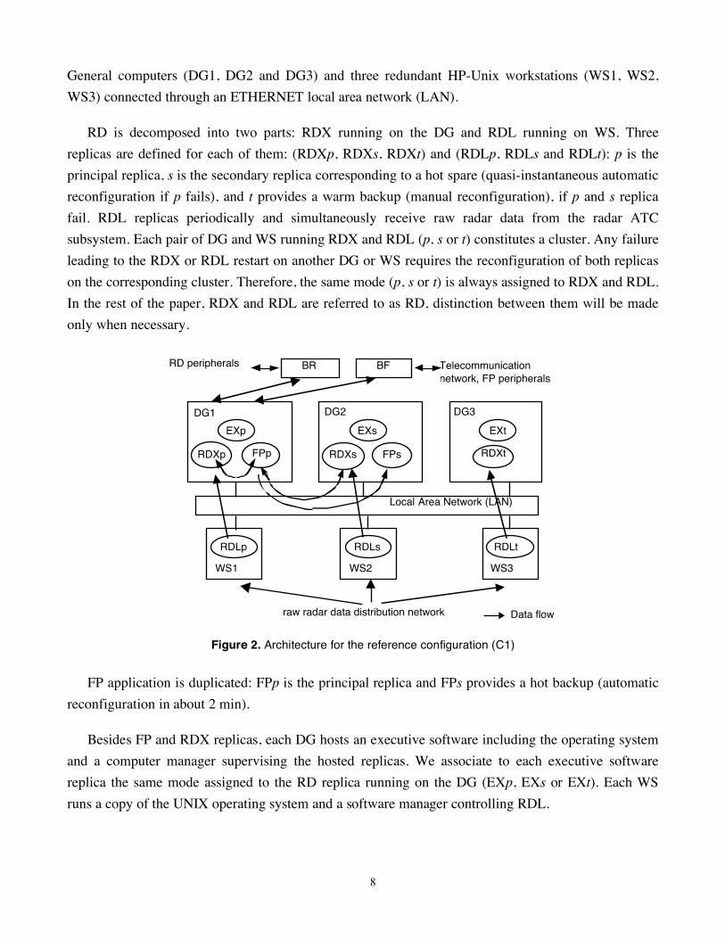
General computers (DG1, DG2 and DG3) and three redundant HP-Unix workstations (WS1, WS2,
WS3) connected through an ETHERNET local area network (LAN).
RD is decomposed into two parts: RDX running on the DG and RDL running on WS. Three
replicas are defined for each of them: (RDXp, RDXs, RDXt) and (RDLp, RDLs and RDLt): p is the
principal replica, s is the secondary replica corresponding to a hot spare (quasi-instantaneous automatic
reconfiguration if p fails), and t provides a warm backup (manual reconfiguration), if p and s replica
fail. RDL replicas periodically and simultaneously receive raw radar data from the radar ATC
subsystem. Each pair of DG and WS running RDX and RDL (p, s or t) constitutes a cluster. Any failure
leading to the RDX or RDL restart on another DG or WS requires the reconfiguration of both replicas
on the corresponding cluster. Therefore, the same mode (p, s or t) is always assigned to RDX and RDL.
In the rest of the paper, RDX and RDL are referred to as RD, distinction between them will be made
only when necessary.
RD peripherals Telecommunication
network, FP peripherals
WS1
RDLp
DG1
EXp
RDXp FPp RDXt
BFBR
Local Area Network (LAN)
Data flowraw radar data distribution network
RDXs FPs
RDLs RDLt
WS2 WS3
DG2
EXs
DG3
EXt
Figure 2. Architecture for the reference configuration (C1)
FP application is duplicated: FPp is the principal replica and FPs provides a hot backup (automatic
reconfiguration in about 2 min).
Besides FP and RDX replicas, each DG hosts an executive software including the operating system
and a computer manager supervising the hosted replicas. We associate to each executive software
replica the same mode assigned to the RD replica running on the DG (EXp, EXs or EXt). Each WS
runs a copy of the UNIX operating system and a software manager controlling RDL.

9
Access to the telecommunication network and to the peripherals providing information display to
the controller and software replica monitoring is performed by two independent I/O boards: BR for RD
and BF for FP. BR and BF implement watchdog mechanisms to supervise the execution of the software
replicas. If p replica is not responding, automatic reconfiguration leads to the assignment of p mode to s
replica and peripherals and communication links connection to the new p configuration. The
architecture described in Figure 2 corresponds to one possible configuration of software replicas on the
DG computers (referred to as the reference configuration). In this configuration, FPp and RDXp run on
the same DG, they exchange information through the LAN for flight plan correlation with radar data.
RDXp receives information from RDLp (running on WS of the same cluster) to display the processed
radar data image. FPp communicates with FPs and RDs to establish checkpoints allowing automatic
reconfiguration of the s replica into p mode in case of failure. There is no need for communication be-
tween RDp and RDs, since both replica receive directly the raw radar data from the radar ATC
subsystem.
Besides this reference configuration (C1), five others are possible as indicated in Table 3.
Transition from one configuration to another may result from system reconfiguration following the
occurrence of a hardware or a software failure. The selection of the new configuration depends on the
type and consequences of failures and on the system components which are still available.
C1 C2 C3 C4 C5 C6
DG1 RDp/FPp RDp/FPp RDs/FPp RDs/FPp RDt/FPp RDt/FPp
DG2 RDs/FPs RDt/FPs RDp/FPs RDt/FPs RDp/FPs RDs/FPs
DG3 RDt RDs RDt RDp RDs RDp
Table 3. Possible RCC configurations
4. The Modeling Approach
The dependability evaluation is based on Markov chains, which are constructed using the modeling
approach, based on Generalized Stochastic Petri Nets (GSPNs), proposed in [9]. In this approach, the
model is built and validated in an incremental manner following a set of construction guidelines. It is
processed by the SURF-2 tool, developed at LAAS-CNRS [3]. This approach provides the users with a
systematic method to handle complex interactions and a large set of failure and recovery assumptions.
In this section, we give the principles of the approach and a brief insight on the construction guidelines.
More details can be found in [8, 9]. This approach is illustrated in Section 5.
Incremental construction of GSPN models. The system model is constructed in several steps. At
the initial step, the system behavior is described taking into account the failures of only one selected

10
component, assuming that the others preserve their operational nominal state. The failures of the other
components are integrated progressively in the following steps of the modeling process. At each step:
1) a new component is added, and 2) the GSPN model is updated and validated (taking into account the
impact of the additional assumptions on the behavior of the components already included in the model).
The validation is done at the GSPN level for structural verification and also at the Markov level to
check the scenarios represented by the model. When the Markov chain is large, the exhaustive analysis
of the chain becomes impractical; sensitivity analyses (using a range of values for model parameters)
are then used to check the model validity.
With the incremental approach, only few additional assumptions are added at each step: the user has
to model only the behavior of the new component and describe how the previous version of the model
has to be modified to account for the interaction of this component with those already integrated. To
ensure better control of the model evolution, we defined a set of guidelines for modeling the
component behavior and their interactions. These guidelines are not mandatory but facilitate
significantly the construction of the model and particularly its validation. Also, they promote reuse of
some parts of the model as the components and the interactions are well identified.
The components' behavior is described by sub-models called modules, while interactions between
components are modeled using module coupling mechanisms. A module describes the behavior of the
component resulting from the occurrence of its internal events (failures, repairs, etc.). It is built of
places, characterizing the states of the component, and transitions, modeling the occurrence of failure
and recovery events specific to that component. The basic rule for the module construction stipulates
that its marking invariant should be equal to 1. To improve the compactness of the module, we
recommend the avoidance of immediate internal transitions (because they generally lead to conflicts
between transitions).
Three basic coupling mechanisms are used to model interactions among components: marking
tests, common transitions and interconnection blocks. The limitation of the type of interaction between
modules aims to ensure better control of model construction and validation.
• Marking tests are used when the occurrence of an event of a given component is conditioned upon the
marking of other component modules. Only stable places of these modules (i.e., those involved in non
vanishing markings corresponding to real component states) can be included in the test. Inhibitor arcs
and bi-directional enabling arcs are used to implement marking tests. Thus, when the internal transition
fires, the marking of the places involved in the test remains unchanged.
• Common transitions are shared by several modules and describe the occurrence of events common to
several components, leading to the simultaneous marking evolution of the involved modules.

11
• The interconnection block models the consequence of the occurrence of an event of an initializing
component in terms of state changes of other target components. These consequences may depend on
the state of components other than those modeled by the initializing and the target modules. A block
connects one or several initializing modules to one or several target modules. It is built of one input
place and a set of immediate transitions. To ensure re-usability and thus improve compactness and
flexibility of the model, generic elementary blocks can be defined to describe specific interactions: for
example, a single block can be defined to stop a software replica, this block is initialized when the
hosting hardware fails or when the operating system fails. The blocks can be connected according to a
parallel-series topology to model a complex interaction. The use of series-parallel sets of elementary
blocks may lead to the simultaneous enabling of several output transitions of different blocks. Priorities
should be defined for the firing of these transitions to avoid conflicts.
5. Modeling of the RCC
There are 17 components to be considered in the RCC model: three RD replicas, three EX replicas,
two FP replicas, two switching I/O boards, three DG computers, three WS computers and the LAN.
Besides the 17 modules modeling these components, an additional one was added (denoted COHAB in
Table 5, Section 5.2) to describe the system configurations (C1 to C6). Following the incremental
approach, the RCC model was built in 18 steps (summarized in Table 5), each one corresponding to the
integration of an additional component. We will illustrate the first four steps corresponding to the
incremental integration of RDp, RDs, RDt and EXt successively. To be able to understand the models,
we first outline the main failure and recovery scenarios assumed when building the RCC model.
5.1. Failure and recovery assumptions
We focus on the failure and recovery scenarios involving RD and EX replicas as they are used in
the rest of this section. To illustrate the complexity of the interactions between RCC components, the
scenarios corresponding to the other components are summarized in Table 4. All these scenarios have
been defined and validated with CAUTRA design and operation teams.
RD replicas. The failure modes and the associated recovery scenarios identified for RD replicas are:
• “RDp local failures” that do not affect RDs. Recovery depends on the availability of RDs or RDt: 1)
If RDs is available (i.e., did not fail due to other reasons), quasi-instantaneous automatic
reconfiguration of RDs into p mode (secpal) followed by I/O links switching via BR, is attempted. If
the latter action fails due to a failure of BR, RDp is restarted on the initial cluster (rstpal); 2) if RDs
is unavailable but RDt is available, a manual reconfiguration of RDt into p mode is attempted using
BR (tstpal); if this action fails, RDp is restarted on the initial cluster.

12
• “RDp and RDs common mode failures”: If RDt is available, tstpal procedure is attempted using BR
followed by rstpal if it fails.
• “ RDs local failures”: Recovered by restarting RDs on the same cluster.
• “ RDt local failures”: Recovered by restarting RDt on the same cluster.
Common mode failures of RDp and RDt manifest only when the manual reconfiguration of t replica
into p mode fails (i.e., when tstpal fails). Therefore, these failures are implicitly included in the failure
mode corresponding to tstpal failure.
Figure 3 describes the above scenarios used to recover from RDp failures (local and common mode
failures), and shows the link with the RD_f failure mode defined in Table 2. Only states 4, 5 and 6
correspond to RD service interruption during more than 30 seconds (RD_f failure mode):~3min are
needed for tstpal execution whereas secpal is quasi-instantaneous.
FP Replicas. Four failure modes are distinguished: FPp local failures. Recovery depends on FPs availability:
1) If FPs is available, automatic reconfiguration of FPs into p mode followed by I/O links switching via BF is
attempted; 2) If FPs is unavailable or reconfiguration fails due to BF, FPp is restarted on the same DG after
elimination, from the system buffers, of some flight plans, suspected to be at the origin of the failure (rstwl). If
rstwl fails, all the flight plans are eliminated and an attempt is made to automatically restore these data from the
adjacent RCCs (dbjx). Otherwise, data are lost, FP is restarted and all the flight plans must be recreated
manually by the controller (dbjn). Each time “dbjx” or “dbjn” are applied, FPs must be restarted after restoring
data from FPp to ensure consistency between both replicas.
FPp & FPs common mode failures. rstwl is attempted first, followed in case of failure by “dbjx” and finally by
“dbjn”.
FPs local failures without significant loss of data. Recovered by FPs restart on the same DG.
FPs local failures with significant loss of data. Recovered by FPs restart after restoring data from FPp.
DG Computers. When a DG fails, the hosted replicas and the computer manager are halted. If FPp or RDp
was running on the DG before failure occurrence, the recovery scenarios described for FPp or RDp are applied
using another DG or another cluster.
WS Computers. The scenario is similar to DG failures, except that only RD replicas are concerned
BF and BR I/O Boards. Two failure modes are distinguished:
Switching failure on demand affecting the failed replica only. It includes non detection of errors requiring s to p
automatic switching, or reconfiguration failure of I/O links. Recovery consists of restarting the failed pal replicas
on the initial DG or cluster. If they are unavailable, BF or BR must be repaired or replaced before FP or RD
restart.
Global failure. This failure may occur at any time and leads to the interruption of all RD or FP replica associated
to the corresponding I/O board. It may be related to a non justified execution of system reconfiguration leading
to the confusion of p, s or t modes assigned to the replicas, or the occurrence of hardware faults leading to the
interruption of all I/O links. RD or FP service can be restored only after the repair of the corresponding I/O
board.
LAN. Several failure modes have been identified for the LAN providing communication support between FP
and RD replicas. These failures may lead to 1) communication loss between RDL and RDX replicas or between
RDp and FPp (if they run on separate DGs), 2) physical isolation of one DG or WS from the rest of the
architecture, or 3) failure of both RD and FP. More details are given in [10].
Table 4. Failure and recovery scenarios associated with FP, DG, WS, BF, BR and LAN components

13
tstpal in
progress
BR switching
in progress
BR switching
in progress
rstpal
in progress
secpal in
progress
RDp OK
RDp local failures(RDs available)
rstpal
success
secpal
failure
success
failure
States 2, 3: No impactStates 4, 5, 6: RD_f
failure
success
RDp local failures
(RDs & RDt unavailable)
or
RDp & RDs common failure
(RDt unavailable)
RDp local failures (RDs unavailable & RDt available)
orRDp & RDs common failure
(RDt available)
1
2 4
3 5
6
Figure 3. Scenarios to recover from failures due to RDp and mapping with RD_f failure mode

14
Besides the software failure modes described above, an additional one has been defined to account
for the software failures leading to RDp and FPp communication loss without interrupting the
execution of these replicas. If FP and RD dialogue is not re-established after RDs reconfiguration to p
mode performed manually by the operator, other procedures are applied leading to the interruption of
flight plan correlation with radar data for more than 5 min (failure mode Com_f in Table 2).
EX replicas. When the executive software fails, the replicas hosted by the DG are halted and the
following recovery actions are done: 1) if the failure is due to the computer manager controlling FP and
RD replicas, the computer manager is reloaded (i.e., reset and restarted); 2) if it is due to the operating
system, DG is rebooted, and the computer manager is restarted. If FPp or RDp was running on the DG,
recovery scenarios implying the reconfiguration of these replicas are applied.
5.2. RCC dependability model
In this section, we explain how we use the incremental modeling approach to build the RCC model
based on the failure and recovery scenarios presented in Section 5.1. We focus on the first four steps
corresponding to the progressive integration of RDp, RDs, RDt and EXt. For each step we describe the
new behavior included in the model due to the integration of a new component.
Step 1: RDp is modeled assuming that the other components are in an operational nominal state
(Figure 4).
RDp local failures (modeled by timed transition loc_Pal) are recovered by the automatic switch of
the RDs into p mode (timed transition secpal). At this step, RDs keeps its initial state, we assume that
the new s replica is restarted instantaneously as soon as the switch of replicas is achieved, and the
switch of I/O links by BR is successful.
RDp
Pal_ok
Pal_secpal
loc_Pal
secpal
Transition Semantics
loc_Pal RDp local failure
secpal RDs switch to p mode
Place Semantics
Pal_ok RDp in "up" state
Pal_secpal RDp waiting for secpal switch
Figure 4. Step 1 (RDp)

15
Step 2: The model is extended by adding the RDs module and updating the RDp module to take into
account the behaviors induced by RDs failures (see Figure 5: the additional places, transitions and
arcs of the new step are plotted in gray and commented below).
At this step, RDp and RDs common failure mode is modeled (timed transition com, shared by mod-
ules RDp and RDs). The firing rates of the transitions corresponding to RDp and RDs common mode
failures and local failures are modeled using the random switch mechanism traditionally used in SPNs.
Place Pal_tstpal and timed transition tstpal, model RDp state during RDt manual switch into p mode.
Some RDp local failures may be recovered by RDs switch to p mode and others by RDt switch to p
mode, depending on RDs availability. This is modeled by transitions loc_Pal, loc1_Pal and the associ-
ated marking tests. To model the fact that RDs is down following the switch of the s replica to p mode,
we use the interconnection block Stp_Sec built up of an input place and two immediate transitions:
stp1s modeling RDs state change from up to down, and stp2s used when RDs is already down when
the failure occurs. These transitions ensure that all RDs states are checked when the block is initialized.
The enabling conditions of stp1s and stp2s are said to be complete and exclusive: when a token arrives
into place Stp_Sec it is immediately consumed and one transition of the block is guaranteed to be fired.
This is a general condition that has to be satisfied by the blocks used to set the target modules into a
given set of states when an event occurs in the initializing module. Ensuring this condition allows the
users to avoid some common modeling errors (e.g. forgetting to test some conditions or building
conflicting immediate transitions), especially when the target modules state space is large, and also
facilitates block reuse. Finally, the marking test on rstsec transition ensures that RDs is restarted after
the restart of RDp.
16
Immediate transition
Timed transition
RDs Sec_ok
Sec_rstsec
loc_Sec
rstsec
RDp Pal_ok
Pal_secpal
loc_Pal
secpal
loc1_Palcom
Pal_tstpal
tstpal
Stp_Sec
stp1sstp2s
Pal_ok RDp in “up” state loc_Pal RDp local failure
(RDs available)
Pal_secpal RDp waiting for secpal
switch
loc1_Pal RDp local failure
(RDs unavailable)
Pal_tstpal RDp waiting for tstpal switch com RDp & RDs common
failure
Sec_ok RDs in "up" state secpal RDs switch to p mode
Sec_rstsec RDs being restarted tstpal RDt switch to pal mode
Stp_Sec Input place of the block used
to stop RDs
stp1s,
stp2s
Transitions of the block
used to stop RDs
rstsec RDs restart
loc_Sec RDs local failure
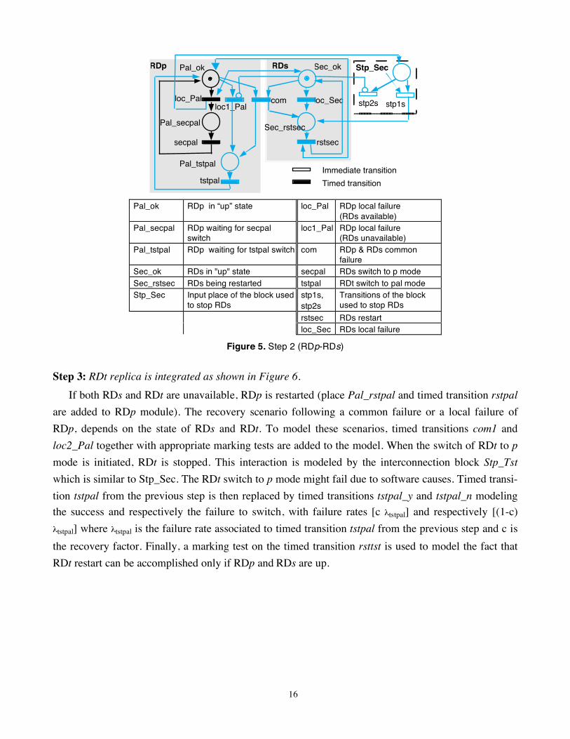
Figure 5. Step 2 (RDp-RDs)
Step 3: RDt replica is integrated as shown in Figure 6.
If both RDs and RDt are unavailable, RDp is restarted (place Pal_rstpal and timed transition rstpal
are added to RDp module). The recovery scenario following a common failure or a local failure of
RDp, depends on the state of RDs and RDt. To model these scenarios, timed transitions com1 and
loc2_Pal together with appropriate marking tests are added to the model. When the switch of RDt to p
mode is initiated, RDt is stopped. This interaction is modeled by the interconnection block Stp_Tst
which is similar to Stp_Sec. The RDt switch to p mode might fail due to software causes. Timed transi-
tion tstpal from the previous step is then replaced by timed transitions tstpal_y and tstpal_n modeling
the success and respectively the failure to switch, with failure rates [c "tstpal] and respectively [(1-c)
"tstpal] where "tstpal is the failure rate associated to timed transition tstpal from the previous step and c is
the recovery factor. Finally, a marking test on the timed transition rsttst is used to model the fact that
RDt restart can be accomplished only if RDp and RDs are up.

17
RDs Sec_ok
Sec_rstsec
loc_Sec
rstsec
RDp Pal_ok
Pal_secpal
loc_Pal
secpal
com
RDt Tst_ok
Tst_rsttst
loc_Tst
rsttst
com1
Pal_rstpal
rstpal
tstpal_n Stp_Tst
stp1tstp2t
Stp_Sec
stp1sstp2s
tstpal_y
loc1_Pal
loc2_Pal
Pal_tstpal
Pal_rstpal RDp being restarted loc2_Pal RDp local failure
(RDt unavailable)
Tst_ok RDt in "up" state com1 RDp & RDs common failure
(RDt unavailable)
Tst_rsttst RDt replica being restarted tstpal_y RDt successful switch to p
mode
Stp_Tst Input place of the block used
to stop RDt
stp1t,
stp2t
Transitions of the block used to
stop RDt
rstpal Restart of RDp
loc_Tst Local failure of RDt
rsttst Restart of RDt
tstpal_n RDt failed switch to p mode
Figure 6. Step 3 (RDp-RDs-RDt)
Step 4: EXt is integrated as shown in Figure 7.
The EXt module accounts for two failure modes: computer manager failure, modeled by timed
transition cm_f and operating system failure, modeled by timed transition os_f. If cm_f occurs, the com-
puter manager is automatically reloaded, and if os_f occurs the executive software should be manually
rebooted and afterwards the computer manager is reloaded. The failure or the stop of EXt leads to the
stop of RDt. This interaction is modeled by initializing the existing block Stp_Tst. Note that reusing the
same block is made possible thanks to transition stp2t that is effectively fired each time the block is
initialized while RDt is already down (e.g., EXt failure while RDt being down).

18
The four steps of RCC model construction described above clearly show that, with the incremental
approach, only a few assumptions are added at each modeling step. Therefore, the incremental
approach allows the users to handle, more easily, the modeling of complex interactions.
rl
EXtEXt_ok
EXt_rb
os_f
EXt_rl
cm_f
rb
RDs Sec_ok
Sec_rstsec
loc_Sec
rstsec
RDp Pal_ok
Pal_secpal
loc_Pal
secpal
com
RDt Tst_ok
Tst_rsttst
loc_Tst
rsttst
com1
Pal_rstpal
rstpal
tstpal_n
Stp_Tst
stp1tstp2t
Stp_Sec
stp1sstp2s
tstpal_y
loc1_Pal
loc2_Pal
Pal_tstpal
EXt_ok EXtst replica in "up" state cm_f Computer manager failure
EXt_rl computer manager being reloaded os_f Operating system failure
EXt_rb Operating system being rebooted rl Computer manager reload
rb Operating system reboot
Figure 7. Step 4 (RDp-RDs-RDt-EXt)
Resulting model. Table 5 gives, for each step of the incremental modeling, the additional component
name accounted for in this step, the size of the GSPN model (number of places and transitions) and the
number of states of the Markov chain. The final model has 116 places and 501 transitions; the
associated reduced Markov chain has 22831 states. State truncation was used starting from step 11 to
reduce the complexity of the Markov chain by eliminating some of the states whose probability of
occupation is non significant. A truncation depth of 4 means that the scenarios constituted by more than
4 successive failures are not considered in the model. This empirical truncation strategy does not
necessarily lead to the elimination of the lowest probability states, however, the ones which are
eliminated are guaranteed to not have a significant impact on the dependability measures (see e.g. [16]
for other truncation algorithms).

19
Step Additional
component
Truncation
depth
# Places #Tran-
sitions
#Markov
states
1 RDp - 2 2 2
2 RDs - 6 9 4
3 RDt - 10 16 10
4 EXt - 13 20 20
5 EXs - 17 36 34
6 EXp - 28 86 42
7 COHAB - 39 110 252
8 FPp - 66 198 880
9 FPs - 72 208 1443
10 BR - 77 220 5751
11 LAN 4 82 235 5173
12 BF 4 87 249 11974
13 DGt 4 90 255 16155
14 DGs 4 99 310 23218
15 DGp 3 109 394 11670
16 WSt 3 112 414 15295
17 WSs 3 114 440 20357
18 WSp 3 116 501 22831
Table 5. Steps of the incremental modeling approach
After each integration step, the model was structurally and semantically validated. In the Markov
chain of a given step, one can identify a sub-chain identical to a sub-chain of the Markov chain
corresponding to the previous step, and which paths have already been validated.
Figure 8 illustrates the semantic validation performed on the Markov chains generated at steps 2
and 3 (bold lines and characters bring out the elements of the chain of step 2, while paths of this chain
that are changed at step 3 are signaled by dotted line in the new chain; for the seek of conciseness the
transition rates are named as the corresponding timed transitions in the GSPN of figure 6).
6. Results
Using the Markov chain generated at the final step of the incremental modeling approach (i.e., step
18), measures UA(X) and W(X) — defined in Section 2 related to the failure modes X identified in
Table 2 ( shaded lines) — have been evaluated. These measures allow comparison of different fault
tolerance strategies of the RCC system as well as the comparison of various strategies for FP and RD
replicas distribution on the DG computers (i.e., the configuration strategies), to identify an optimal
solution.

20
Notation State semantics
1 Pal_ok, Sec_ok, Tst_ok
2 Pal_secpal, Sec_rstsec, Tst_ok
3 Pal_tstpal, Sec_rstsec, Tst_ok
4 Pal_ok, Sec_rstsec, Tst_ok
5 Pal_rstpal, Sec_rstsec, Tst_ok
6 Pal_rstpal, Sec_rstsec, Tst_rsttst
7 Pal_tstpal, Sec_rstsec, Tst_rsttst
8 Pal_ok, Sec_rstsec, Tst_rsttst
9 Pal_ok, Sec_ok, Tst_rsttst
10 Pal_secpal, Sec_rstsec, Tst_rsttst
tstpal_yloc_Tst
loc_Pal
Rst_Pal
com
loc1_Pal
tstpal_n
tstpal_n
loc_Tstloc_Tst
com
loc_Secsecpal
loc_Tstrstpal
loc_Tst
secpal
rstsec
loc_Sec
tstpal_y
tstpal
rsttst
loc_Pal
rstsec
10 9 8
7
654
2 1 3
Figure 8. Markov chain of step 3 corresponding to the GSPN of figure 6
Sensitivity analyses with respect to the most significant reliability parameters (considering different
parameter values) are then performed for the optimal architecture. The objectives are to identify: 1) the
components whose reliability improvement have the most important impact on air traffic safety, and 2)
the parameters on which operational reliability data collection should focus in the future. For the
evaluation purpose, the hardware reliability parameters were obtained from the equipment providers,
while some of the software reliability data items were collected during the RCC operation. When the
numerical values of the parameters were not available, they have been evaluated using data available
on similar systems [4, 15, 19]. The uncertainty was accounted for by performing sensitivity analysis
with respect to the main reliability parameters.
We illustrate the RCC system evaluation results by presenting the influence of configuration
strategies and the impact of the RD fault tolerance strategies on the RCC measures. Additionally, we
give examples of results concerning the global measures of the CAUTRA.
6.1. Influence of RCC configuration strategies
Dependability measures UA(X) and W(X) have been computed for the six configuration strategies
(C1-C6) defined in Table 3. Besides measures corresponding to the six failure modes X defined in
Table 2 (shaded lines) an additional one is computed, denoted “FP_all”, gathering all possible FP
failure modes, including those without significant impact on traffic safety but that significantly
contribute to the service unavailability, bothering the controllers. Also, the definition of FP_all allowed
us to compare our modeling results with data available from the field, which do not distinguish
between FP failure modes. The results are given in Table 6 in which the shaded lines give the values of
the corresponding measures observed during one year of operation of the five RCCs. The relative low
difference between the observed and the evaluated values strengthens our confidence in the validity of
the evaluation. Moreover, our estimations are pessimistic, which is preferable to optimistic estimations.

21
These estimations were also completed by sensitivity analyzes to evaluate the impact on the results of
the main reliability parameters.
UA(X) [minutes/year] C1, C2 C3 - C6 W(X) [1/year] C1, C2 C3 - C6
UA(Com_f) 31.8 188.4 W(Com_f) 0.02 1.76
UA(FP_hd) 16.9 16.9 W(FP_hd) 1.01 1.01
UA(FP_ld) 113.2 113.1 W(FP_ld) 9.83 9.82
UA(FP_tl) 3.8 3.7 W(FP_tl) 0.12 0.12
Observed M1 - 123.3
(C3 only)
UA(RD_f) 12.6 12.6 W(RD_f) 1.21 1.20
Observed UA(RD_f) - 10.5
UA(RD_f!FP_tl) 1.8 10-4
2.610-4
W(RD_f!FP_tl) 210-5
1.510-5
UA(FP_all) 206.0 205.9 W(FP_all) 47.02 47
Observed UA(FP_all) - 202
M1 = [UA(FP_tl) + UA(FP_hd) +UA(FP_Id)]
Table 6. RCC measures for the six RCC configurations
The evaluation results presented in Table 6 show that two classes of configuration strategies can be
distinguished. The difference between these classes is due to the way the communication between RDp
and FPs is accomplished for flight plan correlation: for (C1 & C2) this communication is internal and
performed locally by the executive software of the DG computer, while for (C3-C6), it is done exter-
nally through the LAN. The main difference is perceived for the measures concerning the “Com_f”
failure mode, corresponding to a degradation level L3. These two classes are compared for different
values of "d", the ratio of the failure rate of the LAN and the failure rate of the internal communication.
The results concerning UA(Com_f) are presented in Figure 9. It can be concluded that the
configuration strategies C1 & C2 are always preferred to (C3-C6); the difference is decreasing with the
improvement of the LAN reliability (decrease of d). This result is consistent with the fact that the LAN
is critical for the communication between FP and RD for configurations (C3-C6).
b - minutes per year
d C1, C2 C3 - C6
0 31.48 31.47
1 31.54 62.85
5 31.79 188.37
10 32.09 345.25
a - probability
7 E-4
5 E-4
6 E-4
4 E-4
3 E-4
2 E-4
1 E-4
0 E+0
d
UA(Com_f)
C3 - C6
C1, C2
1086420
Figure 9. UA(Com_f) as a function of d

22
6.2. Influence of the RD fault tolerance strategies
A different fault tolerance strategy could be envisaged for the RD system, by transforming the
warm spare RDt into a cold one (this would allow to continuously use the third cluster for testing new
versions of RD software, but it would take more time for switching from RDt to RDp). The only
measures that are affected concern RD_f. Figure 10 presents the results for both strategies, for different
values of the RD software failure rate, "RD (the shaded line corresponds to the nominal value of "RD).
Note that, compared to the warm RDt spare, a cold one implies a higher unavailability with respect
to the RD_f failure mode. The unavailability increase is greater if the RD software failure rate is
significantly higher than the nominal assumed value. Variation of other reliability parameters has no
significant influence on the difference between these measures for the two strategies. Note that, for
both strategies, UA(RD_f) is highly sensitive to the value of RD software failure rate.
a - probability
b - minutes per year
!RD[1/h] cold warm
10-4 9.36 9.3
10-3 13.22 12.59
10-2 52.08 45.76
cold
strategy
warm
strategy!RD [1/h]
1 E-21 E-4 1 E-3
2 E-5
0 E+0
6 E-5
4 E-5
1 E-4
8 E-5
Figure 10. UA(RD_f) as a function of "RD, for both RD fault tolerance strategies
6.3. Global measures
By combining partial dependability measures evaluated for the CAUTRA subsystems (as shown in
the Appendix), we computed the global dependability measures UA_Ln and W_Ln, defined with
respect to the significant degradation levels Ln, n = [1,… 4] introduced in Table 1.
In the sequel, we first analyse the influence of the RCC configuration strategies on the global
measures, then we evaluate these measures for a reference CAUTRA architecture to give an idea about
the influence of the CAUTRA on air traffic safety.
Comparison of RCC configurations. Considering the six RCC configuration strategies, the main
difference in the global measures is perceived for L3. This is due to the fact that changing the
configuration strategy impacts only the RCC measures concerning the "Com_f" failure mode, which
involves a degradation level L3. The results for UA_L3 and W_L3 are given in Table 7 where UA_L3
and W_L3 are to be compared respectively with UA(Com_f) and W(Com_f) of Table 6. If we compare
the second configuration class with the first one, UA(Com_f) is multiplied by 6 and W(Com_f) by

23
about 100, while the corresponding global measures are only multiplied by 2 and 1.125 respectively.
This is due to the important contribution of other RCC failure modes (FP_hd and FP_ld) as well as to
the contribution of the other CAUTRA subsystems to the L3 global measures. The significant influence
of the RCC configuration is thus smoothed when considering the global measures. However, it is still
important as the unavailability is multiplied by 2.
C1, C2 C3 - C6
UA_L3 [minutes / year] 826.70 1609.60
W_L3 [1 / year] 56.44 63.72
Table 7. UA_L3 and W_L3 values for RCC configurations
Measures of a reference configuration. Considering a reference configuration for each CAUTRA
subsystem (the COC and the five RCC) and the nominal values for the model parameters, we evaluate
the CAUTRA unavailability and the asymptotic frequency for the four service degradation levels.
Table 8 gives these measures:
• Fortunately, the most critical service degradation levels (L1 and L2) are not very frequent and their
duration is very short. This means that CAUTRA failures have very small impact on air traffic
safety.
• The most frequent service degradation level is L3, due to the fact that several single failure modes
lead to L3.
• The very low values of unavailability and frequency corresponding to L4 are due to the fact that
only two failure modes are concerned. Moreover, they are both related to the centralized system IFP
(IFP_ld failure mode) and to the connection of this system with the telecommunication network, TN
(see Table 2) whose functions are less critical.
UA_Ln W_Ln
Probability [min/an] [1/hour] [1/year]
L1 2.28E-09 0.0012 1.31E-08 0.00011
L2 1.60E-04 84.1 7.69E-04 6.73
L3 1.57E-03 826.7 6.44E-03 56.44
L4 2.75E-05 14.4 7.75E-05 0.67
Table 8. Global measures of the reference configuration
7. Conclusions
This paper summarizes the results of a case study dealing with the analysis and evaluation of the
impact of CAUTRA failures on air traffic safety. The effects of these failures on the service delivered
to the controllers to ensure traffic safety are grouped into five degradation levels. To be able to evaluate

24
the system dependability with respect to these levels and to master the model complexity, we have
applied a GSPN-based modeling approach presented in [9] which consists in modeling the system as a
set of modules interconnected via coupling mechanisms describing interactions between components.
The model is constructed in several steps following an incremental approach. Each step integrates the
failure and recovery assumptions of an additional component and updates the model obtained in the
previous step by modeling the impact of the new component on the behavior of those already
considered by the model.
Thanks to this approach, we were able to build and validate complex models of several thousands of
Markov states for the CAUTRA. The results allowed us to analyze several configurations of the
CAUTRA architecture and to identify improvement areas to reduce the impact of CAUTRA failures on
air traffic safety. The architecture was modeled at a level of detail that made it possible to assess the
impact of software and hardware failures, considering different levels of service degradation.
Sensitivity analyses with respect to dependability parameters were also performed. Only some results
concerning the RCC subsystem could be discussed in the paper. They show that the main variation in
dependability measures is related to: 1) communication failures between Radar Data processing and
Flight Plan processing replicas, and 2) software failure rate of Radar Data processing replicas. The
impact of communication failures is minimized when these replicas run on the same cluster compared
to the case where communication is performed via an external network. This result is in agreement with
the previous study we have done on a former architecture of the CAUTRA where only service
unavailability was analyzed without considering different levels of service degradation [18]. Moreover,
the measures derived from our models compare well with those observed on the CAUTRA system
which is currently in operation.
On one hand, our study allowed us to provide feedback to the CAUTRA development and operation
teams. On the other hand, it gave us the opportunity to experiment the applicability of the modeling
approach presented in [9] to a complex real-life system. One possible extension of this work is to
analyze the impact of CAUTRA failures on air traffic performance. Indeed, the occurrence of
CAUTRA failures leads, in some situations, to air traffic limitations and delays. The same modeling
framework could be used, by including reward parameters characterizing performance degradation for
different failure and recovery scenarios.
References
[1] E. Amadio, P. Iaboni, M. Lamanna, et al., “Implementation of High-Availability Mechanisms in the Air
Traffic Control SIR-S System,” 24th Int. Sym. on Fault-Tolerant Computing (FTCS-24), Austin, TX, USA,
1994, pp. 134-136.
[2] A. Avizienis and D. E. Ball, “On the Achievement of a High Dependable and Fault-Tolerant Air Traffic
Control System,” IEEE Computer, vol. 2, pp. 84-90, 1987.

25
[3] C. Béounes, M. Aguéra, J. Arlat, et al., “SURF-2: A Program for Dependability Evaluation of Complex
Hardware and Software Systems,” 23rd Int. Sym. on Fault-Tolerant Computing (FTCS-23), Toulouse,
France, 1993, pp. 668-673.
[4] X. Castillo and D. P. Siewiorek, “Performance and Reliability of Digital Computing Systems,” 25th Int.
Symp. on Fault-Tolerant Computing (FTCS-25), Pasadena, CA, USA, 1995, pp. 367-372.
[5] G. Ciardo and K. S. Trivedi, “A Decomposition Approach for Stochastic Reward Net Models,” Performance
Evaluation, pp. 37-59, 1993.
[6] F. Cristian, B. Dancey, and J. Dehn, “Fault Tolerance in the Advanced Automation System,” 20th Int. Sym.
on Fault-Tolerant Computing (FTCS-20), Newcastle, UK, 1990, pp. 6-17.
[7] B. Dugan, S. J. Bavuso, and M. A. Boyd, “Dynamic Fault-Tree Models for Fault-Tolerant Computer
Systems,” IEEE Transactions on Reliability, vol. 41, pp. 363-377, 1992.
[8] N. Fota, “Incremental Specification and Construction of Dependability Models - Application to CAUTRA
Air Traffic Control Computing System,” PhD, INPT, LAAS Report 97-151, 1997 (in French).
[9] N. Fota, M. Kaâniche, and K. Kanoun, “A Modular and Incremental Approach for Building Complex
Stochastic Petri Net Models,” 1st Int. Conference on Mathematical Methods in Reliability (MMR'97),
Bucharest, Romania, 1997, pp. 151-158.
[10] N. Fota, M. Kaâniche, K. Kanoun, et al., “Dependability Global Modeling and Evaluation of the CAUTRA
System,” , LAAS Report 97-172, 1997 (in French).
[11] N. Fota, M. Kaâniche, K. Kanoun, et al., “Safety Analysis and Evaluation of an Air Traffic Control
Computing System,” 15th Int. Conf. on Computer Safety, Reliability and Security (SAFECOMP'96), Vienna,
Austria, 1996, pp. 219-229.
[12] J. M. Garot and T. Hawker, “Evaluating Proposed Architectures for the FAA's Advanced Automation
System,” IEEE Computer, vol. 2, pp. 33-45, 1987.
[13] K. K. Goswami, R. K. Iyer, and L. Young, “DEPEND: A Simulation-Based Environment for System Level
Dependability Analysis,” IEEE Transactions on Computers, vol. 46, pp. 60-74, 1997.
[14] A. Goyal and S. S. Lavenberg, “Modeling and Analysis of Computer System Availability,” IBM Journal of
Research and Development, vol. 31, pp. 651-664, 1987.
[15] J. Gray, “Why Do Computers Stop and What Can be Done About it?,” 5th Int. Symp. on Reliability in Dis-
tributed Software and Database Systems, Los Angeles, CA, USA, 1986, pp. 3-12.
[16] B. R. Haverkort, “Approximate Performability and Dependability Analysis using Generalized Stochastic
Petri Nets,” Performance Evaluation, pp. 61-78, 1993.
[17] K. Kanoun and M. Borrel, “Dependability of Fault-Tolerant Systems - Explicit Modeling of the Interactions
between Hardware and Software Components,” IEEE Int. Computer Performance & Dependability Sym.
(IPDS'96), Urbana-Champaign, IL, USA, 1996, pp. 252-261.
[18] K. Kanoun, M. Borrel, T. Morteveille, et al., “Modeling the Dependability of CAUTRA, a Subset of the
French Air Traffic Control System,” 26th Int. Sym. on Fault-Tolerant Computing (FTCS-26), Sendai, Japan,
1996, pp. 106-115.
[19] I. Lee and R. K. Iyer, “Software Dependability in the Tandem Guardian System,” IEEE Transactions on
Software Engineering, vol. 21, pp. 455-467, 1995.
[20] M. Malhotra and K. S. Trivedi, “Power-Hierarchy of Dependability-Model Types,” IEEE Transactions on
Reliability, vol. 43, pp. 493-502, 1994.
[21] A. L. Reibman and M. Veeraraghavan, “Reliability Modeling: An Overview for System Designers,” IEEE
Computer, vol. 24, pp. 49-57, 1991.

26
[22] W. Sanders and J. Meyer, “Reduced Base Model Construction for Stochastic Activity Networks,” IEEE
Journal on Selected Areas in Communications, vol. 9, pp. 25-36, 1991.
[23] S. Visram, W. Artner, and P. Marsden, “Safety Case for the NERC Air Traffic Control System,” 15th Int.
Conf. on Computer Safety, Reliability and Security (SAFECOMP'96), Vienna, Austria, 1996, pp. 346-361.

27
APPENDIX: Global measures evaluation
As dependencies between the CAUTRA subsystems (COC, the five RCCs and the
telecommunication network) are weak, the partial measures related to the various subsystems can be
combined to obtain the global ones using of a fault-tree like, combinatorial model.
In this Appendix, we focus on unavailability measures, UA. The asymptotic frequency, W, is
obtained in a similar manner.
UA_Ln are evaluated by combining the partial measures UA(X) as follows:
UA_Ln # UA(s) + UA(d)DoubleFM
!SingleFM
!
where s stand for single failure modes and d for combinations of failure modes, leading to Ln
degradation level.
Suppose that failure mode d represents the combination of single failure modes s1 and s2. The
following apply:
UA(d) = UA(s1!s2) = UA(s1) UA(s2)
where UA(s1) and UA(s2) are evaluated independently from different models, except for the
combinations of failure modes involving the RD and the FP systems of a same RCC. In this case,
UA(d) is evaluated directly from the Markov model of the RCC as performed in Section 5.2.
Table A1 gives the equations for UA. The formulation is directly based on the analysis presented in
Table 2. For example, for L1, only two failure modes are identified: RD_f!IFP_tl and RD_f!FP_tl.
• UA(RD_f!IFP_tl) is computed by multiplying the unavailabilities related to failure modes RD_f
and IFP_tl evaluated respectively from the Markov models of RCC and IFP.
• as RD_f!FP_tl concerns only combination of failures of RD and FP of the same RCC, it is derived
from the RCC Markov model.
The sum accounts for the fact that there are 5 RCCs.

28
UA_L 1 # 5 [UA(RD_f!IFP_tl) + UA(RD_f!FP_tl)] # 5 UA(RD_f) UA(IFP_tl) + 5 UA(RD_f!FP_tl)
UA_L 2 # UA(IFP_tl) + 5 [UA(FP_tl) + UA(RD_f) + UA(FP_hd!IFP_ld) +UA(FP_hd!IFP_hd)+
+ UA(FP_hd !IFP-TN_f) + UA(FP_hd ! TN_f) +UA(FP_hd!FP-TN_f)]
# UA(IFP_tl) + 5 [UA(FP_tl) + UA(RD_f)] + 5 UA(FP_hd) [UA(IFP_ld) + UA(IFP_hd) +
+ UA(IFP-TN_f) + UA(TN_f) + UA(FP-TN_f)]
UA_L 3 # UA(IFP_hd) + UA(TN_f) + 5 [UA(Com_f) + UA(FP_ld) + UA(FP_hd) + UA(FP-TN_f)]
UA_L 4 # UA(IFP_ld) + UA(IFP-TN_f)
Table A1. Equations of global measures UA_Ln