Dependence of lead time on batch size studied by a system

HAL Id: hal-00607163https://hal.archives-ouvertes.fr/hal-00607163

Submitted on 8 Jul 2011

HAL is a multi-disciplinary open accessarchive for the deposit and dissemination of sci-entific research documents, whether they are pub-lished or not. The documents may come fromteaching and research institutions in France orabroad, or from public or private research centers.

L’archive ouverte pluridisciplinaire HAL, estdestinée au dépôt et à la diffusion de documentsscientifiques de niveau recherche, publiés ou non,émanant des établissements d’enseignement et derecherche français ou étrangers, des laboratoirespublics ou privés.

Dependence of lead time on batch size studied by asystem dynamics model

Nabil Mikati

To cite this version:Nabil Mikati. Dependence of lead time on batch size studied by a system dynamics model.International Journal of Production Research, Taylor & Francis, 2010, 48 (18), pp.5523-5532.�10.1080/00207540903164628�. �hal-00607163�

https://hal.archives-ouvertes.fr/hal-00607163

https://hal.archives-ouvertes.fr

For Peer Review O

nly

Dependence of lead time on batch size studied by a system

dynamics model

Journal: International Journal of Production Research

Manuscript ID: TPRS-2009-IJPR-0128.R1

Manuscript Type: Original Manuscript

Date Submitted by the Author:

29-Jun-2009

Complete List of Authors: Mikati, Nabil; XLNT Performance

Keywords: BATCH SIZING, LEAD-TIME REDUCTION, SIMULATION

Keywords (user): SYSTEM DYNAMICS

http://mc.manuscriptcentral.com/tprs Email: [email protected]

International Journal of Production Research

For Peer Review O

nly

Dependence of lead time on batch size studied by a

system dynamics model

Nabil Mikati∗

XLNT Performance

Tranbärsstigen 16E, Strängnäs, Sweden

∗ Email: [email protected]

Page 1 of 16



123456789101112131415161718192021222324252627282930313233343536373839404142434445464748495051525354555657585960

For Peer Review O

nly

Dependence of lead time on batch size studied by a

system dynamics model

Nabil Mikati∗

XLNT Performance

Tranbärsstigen 16E, Strängnäs, Sweden

Most planning models treat lead time as a constant independent of workload, but the resulting order rate implies capacity

utilization which in its turn affects the lead time. An important factor that determines production order rate is the batch

size, one expects therefore a relationship between batch-sizing and lead time. This dependency is examined for different

operational conditions using system dynamics simulation of a manufacturing model comprising a quality control unit

which is also the bottleneck of the system. It is shown that there is an optimal batch size that results in a minimum lead

time and that inventory level at optimum matches desired inventory. Below optimal batch, lead time increases sharply

due to congestion at the bottleneck. The reported results have implications for production planning and implementation

of process improvement.

Keywords: lead time, optimal batch size, system dynamics, simulation, production policies, capacity utilization

∗ Email: [email protected]

Page 2 of 16



123456789101112131415161718192021222324252627282930313233343536373839404142434445464748495051525354555657585960

For Peer Review O

nly

1. Introduction

Lead time1 is a key performance indicator which besides being a crucial measure of service levels is

the only parameter in the objectives scheme described by Hopp and Spearman (2000, P. 196) that

supports both lower manufacturing costs and high sales. Hence insight on how lead times might vary

with factors such as arrival rate, variability and batch size is essential for effective planning and

scheduling. The dependency on batch size is especially important given that in many optimising

models for example the Economical Order Quantity, Penido 2007, or using Material Requirement

Planning (MRP) procedures, lead times are treated as a constant independent of planning policy.

In this work system dynamics (SD) simulation is used to investigate lead times in a manufacturing

environment where one of the processing units is a bottleneck. Similar workflows are found in the

pharmaceutical and chemical industries where semi-finished products have to undergo thorough

testing before being packaged and released to the market. It is often the case, especially in

pharmaceutical manufacturing, that quality testing is time consuming, labour intensive and

administered by a unit independent from production although from the perspective of supply chain it

is an integral part of the workflow. When demand increases planers feel the pressure to send more

orders into production thereby risking congestion at the bottleneck and ending up in long queues and

delays.

1.1 Related work

Karmarker 1987, 1993 examined the relationship between lot-sizing and lead times from the

perspective of queue theory. He showed that as batch sizes are reduced, utilization i.e. the ratio

between arrival rate and throughput approaches unity, the average time an item spends in the system

increases very rapidly. At the other end of the scale as batch size increases, waiting times dominate

the process and the average lead time starts to increase. In between there is a minimum lead time.

Hopp and Spearman (2000, P. 305) computed optimal batch sizes for different batching processes.

Their results are similar to those of Karmarker cited above. Gung 1999 considered the effect of set

up time and batch size reduction on lead times. The author describes a workload balancing model

and suggests a minimum set up time reduction ratio. Chandra and Gupta 1997 studied lead time

reduction in a semiconductor facility where batch processing is a part of the manufacturing line.

They outline a procedure whereby the bottleneck station pulls its requirements from the assembly

section. Lee and Chung 1998 investigated batching decisions in a multi product environment. They

used a non linear mixed integer program to minimize the flow in a closed job shop. Enns 2001

analysed the relation between planned lead times and batch size in the context of MRP logic. Olinder

and Olhager 1998 studied the effect of different lot sizing models controlled by MRP logic on lead

times. Ocrun et al. 2006 compared a number of capacity models using system dynamics simulations.

The authors conclude that at high utilization many models used in production planning and system

dynamics fail to capture the non-linear behaviour involved, while a saturated concave clearing

function2 does. Recently Pahl et al. 2007 reviewed different models of load dependent lead times in

1In this work lead time is taken to be the average time from order arrival to shipping

2 More on clearing functions in section 2.1, for details see Pahl et al. 2007

Page 3 of 16



123456789101112131415161718192021222324252627282930313233343536373839404142434445464748495051525354555657585960

For Peer Review O

nly

the context of production planning.

1.2 System Dynamics

System Dynamics is a method for analysing policies and solving complex problems by using

computer simulation models. The models capture the causal interlinks within the system and project

them as a structure of feedback loops. The use of SD in Supply Chain Management is dated back to

the seminal work of Forrester 1958, 1961 and it has been applied to a wide range of problems related

to manufacturing and supply chain management Sterman 2000, Angerhofer and Angelides 2000,

Akkermans and Dellaert 2005, Min Huang et al. 2007. SD takes an aggregate view on policies, the

level of aggregation and the boundary of the model should reflect the time scale for the dynamics of

interest and the problem studied.

2. Production Model

An overview of the manufacturing model is shown in Figure 1, some links are omitted in order to

simplify the sketch. The model is adapted from the generic structure by (Sterman 2000 chap. 18),

neglecting those elements of the supply chain that deals with procurement or administrative delays

since the concern of the study is the effects of batch-sizing on lead time. The simulation experiments

were performed using VENSIM software. Further details regarding the underlying equations are

given in the appendix.

Figure 1

Orders arrive continuously and batching is accomplished using DELAY BATCH function which

takes a continuous input stream and returns it as pulses when the amount accumulated is equal to the

specified batch size. Following the first manufacturing stage (production) a given number of samples

are sent for quality testing. Meanwhile semi-finished products are kept in quarantine pending release.

When quality control is completed, finishing (packaging, labelling etc.) is carried out and products

are sent to finished goods inventory for delivery. Unfilled orders are backlogged and lead time is

calculated from

lead time = backlog/ order fulfilment rate (1)

For an order rate D and batch size Q, the waiting time to reach Q is Q/D, also the frequency of

sample arrivals to quality control is ND/Q, where N is the number of samples sent to quality control

for every batch produced. Hence decreasing batch size shortens the waiting time but increases the

load on the bottleneck causing congestion and delays. Increasing Q will have the opposite effect. An

intermediate batch size results in a minimum lead time.

2.1 Delays at the Work Centres

The outflow from stocks is described by first order material delay (Sterman 2000 p. 415)

Outflow = WIP/delay time (2)

Page 4 of 16



123456789101112131415161718192021222324252627282930313233343536373839404142434445464748495051525354555657585960

For Peer Review O

nly

The delay time at Production and Finishing is set to 0.5 weeks irrespective of batch size. In the range

of batch sizes considered this a reasonable assumption since many facilities may have additional

capacity. More importantly, making the delays at these work centres time dependent will have little

effect on the main results as long as these delays are kept shorter than the delay at the bottleneck.

The output rate at the bottle neck is taken to be labour constrained which is a common situation in

control laboratories. Maximum throughput becomes

p is the productivity (samples cleared by unit labour), w the workforce and T0 is the raw process

time, i.e. the time it takes to perform quality control when there is ample capacity and no congestion

and W0 = pw is the critical WIP level.

The delay time at quality control is modelled using the concepts of best-case performance and

practical worst-case performance (PWC), two special cases described by Hopp and Spearman 2000

for a balanced line consisting of a number of single machines. Best case performance is the scenario

where there is no process variation. The delay time is constant up to a point where load is equal W0.

Beyond that point delay time increases proportionally with the load. It should be noted that the

absence of variability referred to does not imply a FIFO discipline in the present study since a first

order material delay assumes mixing of the units in the stock; it is rather referring to the regularity of

processing times of the samples. The equations for the outflow rate and delay time for best-case

performance are

Practical worst-case performance describes the situation where there is a maximum randomness in

the system and every possible state has the same probability, for example presence or absence of

labour occurs with the same frequency.

The outflow rate and delay time are

(4)

(5)

(6)

(3)

(7)

Page 5 of 16



123456789101112131415161718192021222324252627282930313233343536373839404142434445464748495051525354555657585960

For Peer Review O

nly

The delay time in this case reduces to its minimum T0 when there is only one sample in transient.

Equations (4) and (6) are examples of the clearing functions mentioned earlier used to model

capacity versus work load. In the terminology of Orcun et al. 2006 these equations correspond to

capacitated constant proportion and concave saturating clearing functions. Karmarker 1993, used an

empirical parameter k in Eq. (6) instead for W0 – 1 to determine the output rate.

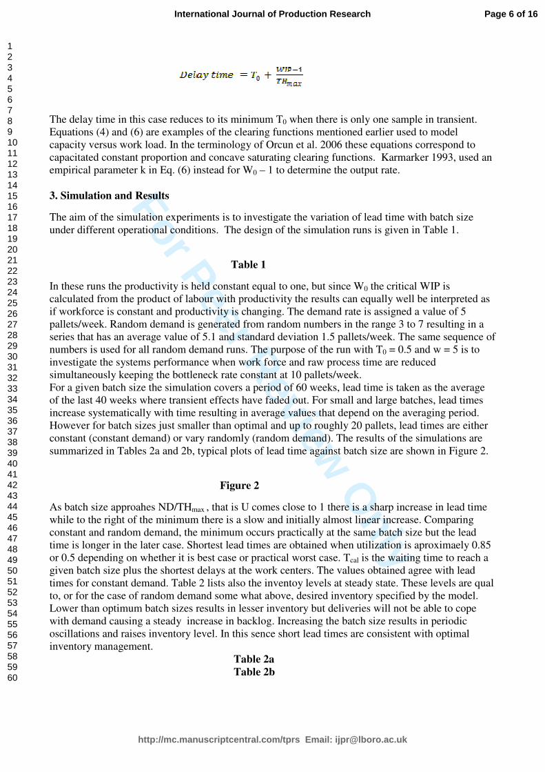
3. Simulation and Results

The aim of the simulation experiments is to investigate the variation of lead time with batch size

under different operational conditions. The design of the simulation runs is given in Table 1.

Table 1

In these runs the productivity is held constant equal to one, but since W0 the critical WIP is

calculated from the product of labour with productivity the results can equally well be interpreted as

if workforce is constant and productivity is changing. The demand rate is assigned a value of 5

pallets/week. Random demand is generated from random numbers in the range 3 to 7 resulting in a

series that has an average value of 5.1 and standard deviation 1.5 pallets/week. The same sequence of

numbers is used for all random demand runs. The purpose of the run with T0 = 0.5 and w = 5 is to

investigate the systems performance when work force and raw process time are reduced

simultaneously keeping the bottleneck rate constant at 10 pallets/week.

For a given batch size the simulation covers a period of 60 weeks, lead time is taken as the average

of the last 40 weeks where transient effects have faded out. For small and large batches, lead times

increase systematically with time resulting in average values that depend on the averaging period.

However for batch sizes just smaller than optimal and up to roughly 20 pallets, lead times are either

constant (constant demand) or vary randomly (random demand). The results of the simulations are

summarized in Tables 2a and 2b, typical plots of lead time against batch size are shown in Figure 2.

Figure 2

As batch size approahes ND/THmax , that is U comes close to 1 there is a sharp increase in lead time

while to the right of the minimum there is a slow and initially almost linear increase. Comparing

constant and random demand, the minimum occurs practically at the same batch size but the lead

time is longer in the later case. Shortest lead times are obtained when utilization is aproximaely 0.85

or 0.5 depending on whether it is best case or practical worst case. Tcal is the waiting time to reach a

given batch size plus the shortest delays at the work centers. The values obtained agree with lead

times for constant demand. Table 2 lists also the inventoy levels at steady state. These levels are qual

to, or for the case of random demand some what above, desired inventory specified by the model.

Lower than optimum batch sizes results in lesser inventory but deliveries will not be able to cope

with demand causing a steady increase in backlog. Increasing the batch size results in periodic

oscillations and raises inventory level. In this sence short lead times are consistent with optimal

inventory management.

Table 2a

Table 2b

Page 6 of 16



123456789101112131415161718192021222324252627282930313233343536373839404142434445464748495051525354555657585960

For Peer Review O

nly

3.1 Relation to Queue theory

Treating quality control as an M/M/1 queuing system (Hopp and Spearman 2000, p. 269) the average

lead time can be written as

the last two terms are due to production and finishing. Equation (8) is graphed in Figure 3, the curve

is similar to those obtained by SD simulation but is less flat.

Figure 3

An expression for the batch size that minimizes T(Q) can be found by taking the derivative and

setting it to zero giving

The second term is due to randomness because Q* = DT0N/W0 is equivalent to 100% capacity

utilization. Eq.(9) gives results that agree well with practical worst-case scenario, for example

substituting the data used to plot Figure 3, Eq. (9) gives 12 pallets as in Table 2.

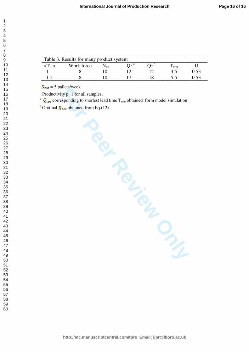
3.2. Many Product System

So far the analysis has been limited to a one product system and samples having identical raw

process time. To model the general case where process times at the testing unit are different (this

may be the case even for a homogenous batch) requires indexing the individual batches as well as the

samples, a procedure that considerably complicates the simulation. Moreover identifying the

individual items raises issues such as scheduling and prioritisation which are beyond the scope of

this work. Nevertheless by expressing the workload in time units it is possible to estimate the degree

of capacity utilization and total batch size resulting in smallest average lead time.

Let be the total demand and the total number of batches. The

proportion of the in individual batches in the production mix should reflect demand i.e. =

otherwise there will be an access inventory of one product and shortage of another. This

production mix generates samples each having a raw process time . In time units

the workload generated is and maximum throughput for sample type j becomes

where p and w are productivity and work force as in Eq.(3). Since

the output is considered to be constrained only by labour sample analysis is carried out in parallel,

hence the maximum total throughput is . If the number of samples exceeds

available workforce than some of the in the summation will be zero. This is equivalent to

assigning some analysts more than one sample and considering these as a single unit of work with a

process time equal to the sum of the individual process times. The summation is then taken over the

number of analysts available. With these definitions Eq.(7) and Eq.(8) can be rewritten as

(8)

(9)

Page 7 of 16



123456789101112131415161718192021222324252627282930313233343536373839404142434445464748495051525354555657585960

For Peer Review O

nly

(10)

(11)

WL is the work load in time units and is the average raw process time.

From Eq.(11) one gets

(12)

Which reduces to Eq.(9) when one item with constant raw process time is considered. Simulation

runs after adapting the model to the definitions above and expressing the delay time by Eq.(10)

generates curves as in Figure 2. Numerical results are reported in Table 3.

Table 3

4. Summery

System dynamics is a useful tool for studying the effectiveness of different policies. The model

presented above reproduces a simple manufacturing system where product must be tested before

being released. The quality control is assumed to be the bottleneck section of the workflow. The

maximum output rate at the testing station is constrained by labour, productivity and raw process

time. In both cases it is shown that as capacity is heavily exploited WIP levels and lead times

increase indefinitely due to congestion at the bottleneck. Also there is an optimum batch size which

results in minimum lead times. These insights are important in two ways. Firstly, constantly pushing

production rate beyond a certain point results in a viscous circle of missed due dates, increased

workload and longer queues. Preliminary Eq.(9), or a utilization level in the range 0.5 to 0.8 can be

used to estimate a passable work load. Secondly, one should take a systemic approach to process

improvement. Streamlining and enhancing the workflow in one sector may turn out to be counter

productive unless measures are also taken to manage the side effects generated at the bottleneck.

Page 8 of 16



123456789101112131415161718192021222324252627282930313233343536373839404142434445464748495051525354555657585960

For Peer Review O

nly

References

Akkerman, H. and Dellaert, N., 2005. The rediscovery of industrial dynamics to supply chain

management in a dynamic and fragmented world. System Dynamics Review, 21(3), 173 – 186.

Angerhofer, B. J. and Angelides, M.C., 2000. System dynamic modelling in supply chain

management: research review. Proceedings of the 2000 Winter Simulation Conference,

342 – 351. Available from http://www.informs-cs.org/wsc00papers/049.PDF [Accessed 14 April

2008].

Chandra, P. and Gupta S.,1997. Managing batch processors to reduce lead time in a semiconductor

Packaging line. International Journal of Production Research, 35(3), 611 – 633.

Enns, S.T., 2001. MRP performance effects due to lot sizes and planned lead time. International

Journal of Production Research, 39(3), 461 – 480.

Gung, R.R.,1999. A work load balancing model for determining set-up time and batch size

reductions in GT flow line work cells. International Journal of Production Research, 37(4),

769 – 791.

Forrester, J.W., 1958. Industrial dynamics: A major breakthrough for decision makers. Harvard

Business Review, 36(4), 37 – 66; 1961, Industrial dynamics. Portland OR: Productivity Press.

Hopp, J.W. and Spearman, M.L., 2000. Factory physics. 2nd ed. Irwin MacGraw-Hill.

Huang M. et al., 2007. Simulation study using system dynamics for a CONWIP-controlled lamp

supply chain. The International Journal of Advanced Manufacturing Technology, 32(1-2),

184 – 191.

Karmarker, U.S., 1987. Lot sizes, lead time and in-process inventories. Management Science, 33(3),

409 – 418, 1993 Manufacturing lead times, order release and capacity loading. In: Handbooks

in OR & MS, 287 – 329.

Lee , J.M. and Chung, C.H., 1998. Batching multiple products on parallel heterogeneous machines in

a closed job shop. International Journal of Production Research, 36(10), 2793 – 2811.

Ocrun, S. et al., 2006. Using system dynamics simulations to compare capacity models for

production planning. Proceedings of the 2006 Winter Simulation Conference, 1855 – 1862,

Available from http://www.informs-sim.org/wsc06papers/237.pdf [Accessed 6 mars 2008].

Olinder, A.M. and Olhager, J., 1998. The effect of MRP lot sizing on actual cumulative lead times

in multilevel systems. Production Planning & Control, 9(3), 293 – 302.

Pahl, J. et al., 2007. Production planning with load dependent lead times: an update of research.

Annals of Operations Research, 153(1), 297 – 345.

Sterman, J.D., 2000. Business dynamics, system thinking and modelling for a complex world.

MacGraw-Hill Higher Education.

Page 9 of 16



123456789101112131415161718192021222324252627282930313233343536373839404142434445464748495051525354555657585960

http://www.informs-cs.org/wsc00papers/049.PDF

http://www.ingentaconnect.com/content/klu/170;jsessionid=8ljalrq8eoii7.alice

http://www.informs-sim.org/wsc06papers/237.pdf

For Peer Review O

nly

Appendix

Further details regarding the model

shipment rate = MIN(desired shipment rate, finished goods inventory/minimum delay time), that is

the firm ships either what it wants or what it is able to.

finished goods inventory (initial value)= customer order rate * minimum delivery delay

order fulfilment rate = shipment rate; formulated as MIN(back log/time step, shipment rate) in order

to prevent the backlog becoming negative

backlog(initial value) = customer order rate * minimum delivery delay

desired shipment rate = customer order rate

minimum delivery delay = delay time production + T0 + delay time finishing

delay time production = delay time finishing = 0.5 weeks

adjustment for inventory = (desired inventory – finished goods inventory)/inventory adjustment time

inventory adjustment time = 4 weeks

expected order rate = SMOOTH(order rate, averaging time), this term calculates a time average

based on an exponential smoothing of the input

averaging time = 4 weeks

desired inventory = expected order rate * minimum delivery delay + safety stock

safety stock = 2.5 pallets

number of samples = 10 samples

Runge-Kutta integration method was used, time step 0.016 week

Page 10 of 16



123456789101112131415161718192021222324252627282930313233343536373839404142434445464748495051525354555657585960

For Peer Review O

nly

Production Unreleased

ProductsFinishing

Finished Goods

Inventory

Quality

Control

production rate production finish

ratefinishing start rate finishing rate

Back Log

customer order

rate

order fulfillment

rate

minimum delivery

delay

lead time

QC start rate release rate

expected order

rate

desired inventory

safety stock

adjustemnt for

inventory

desired production

inventory

adjustement time

averaging time

delay time

production

delay time finishing

batch size

number of samples

CT work force

desirede

shipment rate

To

max throughput

productivity

shipment rate

Figure 1. Stocks and flow structure of the manufacturing model studied

Page 11 of 16



123456789101112131415161718192021222324252627282930313233343536373839404142434445464748495051525354555657585960

For Peer Review O

nly

(a) (b)

Figure 2. Lead time vs. batch size, (a) best-case, (b) practical worst case. For both runs w = 8, P = 1, T0 = 1

Page 12 of 16



123456789101112131415161718192021222324252627282930313233343536373839404142434445464748495051525354555657585960

For Peer Review O

nly

Figure 3. Plot of Eq.(8) for N = 10, D = 5, THmax = 8, T0=1

Page 13 of 16



123456789101112131415161718192021222324252627282930313233343536373839404142434445464748495051525354555657585960

For Peer Review O

nly

Table 1. Design variables and their attributes

Work force Delay time Demand T0

10 Equations (5) and (7) Constant and random 1



5 Equations (5) and (7) Constant and random 0.5

Page 14 of 16



123456789101112131415161718192021222324252627282930313233343536373839404142434445464748495051525354555657585960

For Peer Review O

nly

Table 2a. Results summery, constant demand

T0 = 1 Work force Q* a

Tmin FGIb

Stdc

Ud

Tcale

Best case 10 6 3.6 12.5 0.0 0.83 3.2

Best case 8 8 3.7 12.5 0.1 0.78 3.6

Best case 6 10 3.9 12.5 0.2 0.83 4.0

PWC 10 11 4.4 12.5 0.2 0.45 4.2

PWC 8 12 4.5 12.5 0.3 0.52 4.4

PWC 6 15 4.8 12.5 0.4 0.56 5.0

T0 = 0.5

Best case 5 6 2.9 10 0.1 0.83 2.7

PWC 5 9 3.4 10 0.1 0.56 3.3 a batch size corresponding to shortest lead time Tmin

b average finished goods inventory at Q*

c standard deviation finished goods inventory

d utilization

e theoretical lead time calculated by Tcal = Q*/D + T0 + 1

Table 2b. Results summery, random demand

T0 = 1 Work force Q* a

Tmin FGIb

Stdc

Ud

Best case 10 6 5.2 13.5 2.2 0.83

Best case 8 7 5.2 13.5 2.3 0.89

Best case 6 9 5.4 13.5 2.2 0.93

PWC 10 10 5.9 13.5 2.3 0.5

PWC 8 12 6.0 13.6 2.3 0.52

PWC 6 14 6.3 13.5 2.1 0.64

T0 = 0.5

Best case 5 6 4.4 10.8 2.1 0.83

PWC 5 7 4.9 10.8 2.2 0.71

Page 15 of 16



123456789101112131415161718192021222324252627282930313233343536373839404142434445464748495051525354555657585960

For Peer Review O

nly

= 5 pallets/week

Productivity p=1 for all samples.

a corresponding to shortest lead time Tmin obtained form model simulation

b Optimal obtained from Eq.(12)

Table 3. Results for many product system

<T0 > Work force Ntot Q* a

Q* b Tmin

U

1 8 10 12 12 4.5 0.53

1.5 8 10 17 18 5.5 0.53

Page 16 of 16



123456789101112131415161718192021222324252627282930313233343536373839404142434445464748495051525354555657585960

Documents

Dependence of lead time on batch size studied by a system