Embed Size (px)
Citation preview
From:OECD Journal on Budgeting
Access the journal at:http://dx.doi.org/10.1787/16812336
Fiscal rules and regime-dependent fiscal reaction functions
The South African case
Philippe Burger, Marina Marinkov
Please cite this article as:
Burger, Philippe and Marina Marinkov (2012), “Fiscal rules andregime-dependent fiscal reaction functions: The South African case”,OECD Journal on Budgeting, Vol. 12/1.http://dx.doi.org/10.1787/budget-12-5k9czxjth7tg

This document and any map included herein are without prejudice to the status of orsovereignty over any territory, to the delimitation of international frontiers and boundaries and tothe name of any territory, city or area.

1
OECD Journal on Budgeting
Volume 2012/1
© OECD 2012
Fiscal rules and regime-dependent fiscal reaction functions: The South African case
by
Philippe Burger and Marina Marinkov*
This article argues the case for a policy of “anchored flexibility” in the form of a flexible fiscal rulethat allows for the pursuit of economic stability but always anchors that pursuit in fiscalsustainability. The rule is explicitly structured to be simple and is designed in analogy to theinflation-targeting framework. The article heeds the warning that consistently forecasting theoutput gap with any degree of precision is quite difficult, if not impossible, and thus proposes atarget band for the deficit, instead of point targets for the overall deficit and the structural budgetbalance. To ensure fiscal sustainability over and above the contribution of the deficit rule, thearticle also proposes a band for the debt/GDP ratio. This debt rule acts as a negative feedbackrule that stipulates the adjustments required in the deficit, should the actual debt/GDP ratiomove outside the stipulated band. Since the government needs to change revenue andexpenditure in order to change the deficit, the article then explores empirically whether and withhow much revenue and expenditure in South Africa changed to maintain fiscal sustainability.More specifically the article explores various models of the fiscal reaction function to illuminategovernment behaviour in South Africa. These models consider how the deficit, expenditure anddifferent types of revenue reacted to the debt/GDP ratio and the output gap to ensure fiscalsustainability. Lastly, the article considers measures that could enhance the automaticstabilisers, while simultaneously allowing for the maintenance of fiscal sustainability in themedium term.
JEL classification: H60, E62, C32
Keywords: fiscal rules, fiscal reaction function, time-series models, South Africa
* Philippe Burger is Professor and Chair of the Department of Economics at the University of the FreeState, South Africa. Marina Marinkov is Senior Researcher at the Macroeconomics and Public FinanceUnit of the Financial and Fiscal Commission (FFC), South Africa. An earlier version of this articlewas presented at the ERSA Workshop on Public Economics (Economic Research Southern Africa,http://econrsa.org) held at the Stellenbosch Institute for Advanced Study on 2-3 May 2011. The authorswish to thank George Kopits, Estian Calitz and Krige Siebrits as well as other participants in the ERSAworkshop for valuable comments. The usual disclaimers apply.

FISCAL RULES AND REGIME-DEPENDENT FISCAL REACTION FUNCTIONS: THE SOUTH AFRICAN CASE
OECD JOURNAL ON BUDGETING – VOLUME 2012/1 © OECD 20122
The financial and economic crisis that started in 2008 as well as the response of
governments to the crisis resulted globally in fast-rising public debt/GDP ratios.
Governments in countries such as Greece, Ireland and Portugal face the possibility of debt
restructuring and bailouts by the EU and the IMF, while countries such as the United
Kingdom and the United States also experienced the sharpest peace-time increase in their
debt/GDP ratios since modern times. Financial markets too express uncertainty, and
several calls have been made in the United Kingdom and the United States to identify an
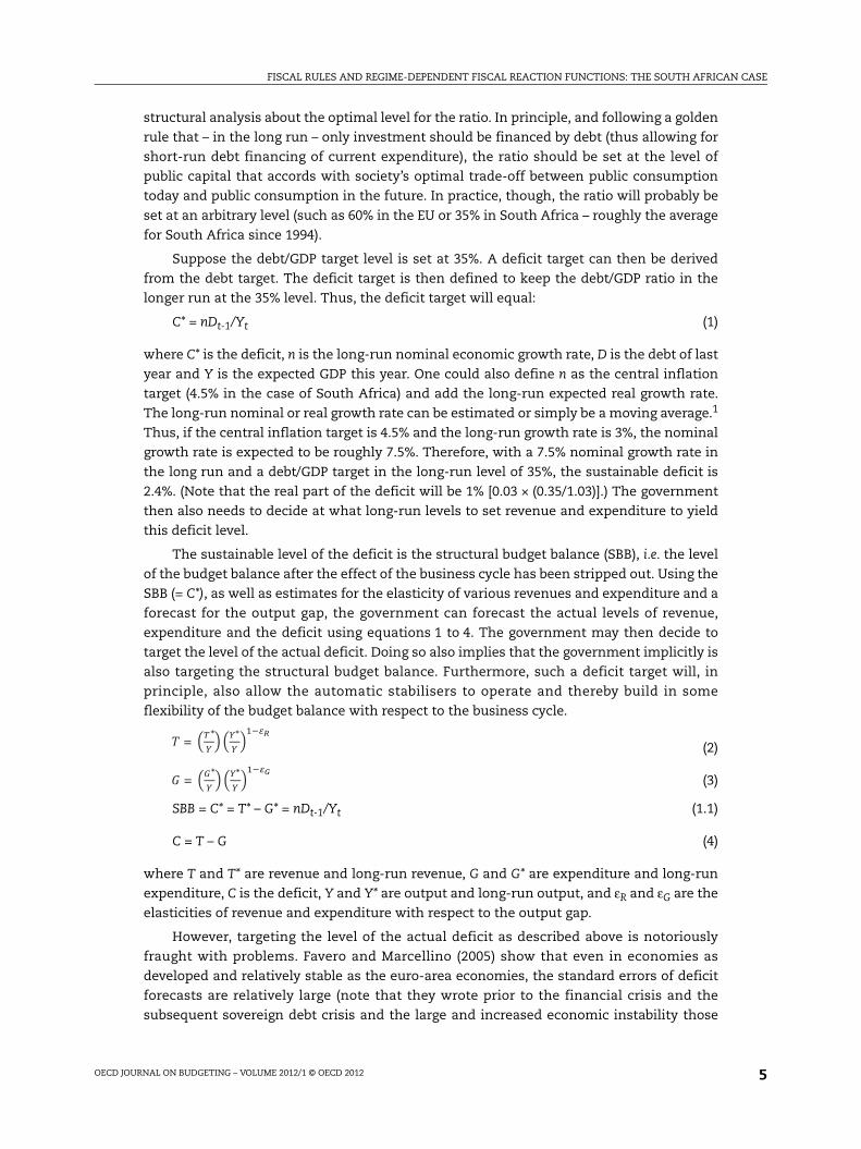
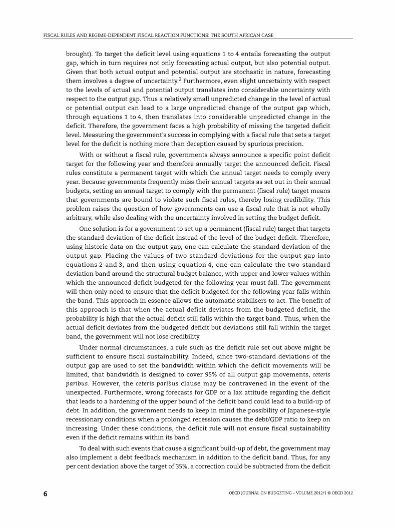
“exit strategy” from the large stimulus policies pursued by their governments. South Africa
also experienced an increase in its public debt/GDP ratio, though the increase is not nearly
as dramatic as in the countries cited above (see Figure 1). These increases in public debt/
GDP ratios globally raise again the question whether flexible fiscal rules are not necessary.
More specifically: Is what is needed not rules that allow for stimulus measures during
recessions, but rules that also identify an exit strategy from these measures? Indeed, if
these exit strategies are clearly defined in terms of a fiscal rule, the stimulus measures
themselves might generate more market confidence and thus have a larger impact.
Therefore, this article argues the case for a policy of “anchored flexibility” in the form
of a flexible fiscal rule that allows for the pursuit of economic stability but always anchors
that pursuit in fiscal sustainability. The rule is explicitly structured to be simple and is
designed in analogy to the inflation-targeting framework. In addition to containing a
proposal for a fiscal rule that describes how the government should react in future, the
article also explores how the government reacted in the past by presenting estimations of
the fiscal reaction function. Various specifications of that function are presented. In
Figure 1. The public debt/GDP ratio in South Africa
Source: South African Reserve Bank.
70
60
50
30
20
10
0
40
1947
1950
1953
1956
1959
1962
1965
1968
1971
1974
1977
1980
1983
1986
1989
1992
1995
1998
2001
2004
2007
2010
Public debt/GDP

FISCAL RULES AND REGIME-DEPENDENT FISCAL REACTION FUNCTIONS: THE SOUTH AFRICAN CASE
OECD JOURNAL ON BUDGETING – VOLUME 2012/1 © OECD 2012 3
addition, the estimated fiscal reaction functions are also used to explore whether revenue
or expenditure carried the largest burden of adjustment in the past. Showing that the
largest adjustments fell on revenue, the article also proposes how expenditure measures
can be augmented to allow for increased sensitivity to recessions, while also creating a
mechanism for a fast adjustment and restitution of fiscal sustainability once the recession
passes.
1. Whence fiscal rules?The debate about fiscal rules is not a recent phenomenon, with the underlying
concern regarding the size and burden of public debt being an age-old one, going back
centuries. For instance, referring to 18th century United Kingdom, David Hume (1742)
stated that “… either the nation must destroy public credit, or public credit will destroy the
nation”. The oldest fiscal rule is the simple balanced budget rule, succinctly stated for the
first time in modern times in the “treasury view” of 1929 (Clarke, 1988). However, the Great
Depression highlighted the untenable nature of this rule during severe recessionary times.
Thus, following the Great Depression, rules gave way to discretionary fiscal policy in the
1940s, 1950s and 1960s. Keynesian economics and Abba Lerner’s “functional finance view”
emphasised that government should not focus on balancing the budget, but rather on
balancing the economy; the budget will then take care of itself (Lerner, 1951). These views
provided the theoretical underpinnings for discretionary fiscal policy.
Discretionary policy seemed to have carried the day in the first three decades
following WWII. The exceptional economic growth rates and the rather low interest rates
meant that governments could grow their economies out of the public debt burdens that
they incurred during WWII. South Africa is no exception, with public debt doubling in
amount during the first three decades, though halving as a ratio of GDP. However, this does
not mean that fiscal rules disappeared altogether. Most governments still followed a basic
public sector golden rule whereby loans were predominantly incurred to finance
infrastructure and capital, while current expenditure was financed by tax revenues. Fiscal
rules also did not disappear from economic literature. As early as 1948, Milton Friedman
argued the case for a flexible fiscal rule that allows for the operation of what is today
known as automatic stabilisers. To quote him: “The principle of balancing outlays and
receipts at a hypothetical income level would be substituted for the principle of balancing
actual outlays and receipts” (Friedman, 1948:249-250). Hence, Friedman’s proposal
essentially aims at balancing the budget over the business cycle.
As Friedman argued, his proposal was not an isolated set of ideas, since it drew on
existing ideas circulating in academic and policy circles at the time. Though Friedman
made his proposal in 1948, fiscal rules only became a serious topic of discussion again in
the 1980s and 1990s, following the significant deficit and debt problems that many
developed countries then faced. By this time, the debate on fiscal rules could also draw on
a significant public choice literature emphasising issues such as time inconsistency in the
behaviour of governments, the deficit bias of governments, and the political business cycle
(cf. Alesina and Perotti, 1994; Corsetti and Roubini, 1996; Drazen, 2004; Kydland and
Prescott, 1977).
Different authors also had different definitions of what constitutes fiscal rules, but all
definitions implied a constraint of fiscal policy actions over time (cf. Buti and Giudice, 2002,
2004; Drazen, 2004; Kell, 2001; Kopits, 2004; Kopits and Symansky, 1998; Milesi-Ferretti,

FISCAL RULES AND REGIME-DEPENDENT FISCAL REACTION FUNCTIONS: THE SOUTH AFRICAN CASE
OECD JOURNAL ON BUDGETING – VOLUME 2012/1 © OECD 20124
2003; Siebrits and Calitz, 2004; and Tanner, 2004). In addition, most authors view fiscal rules
as restrictions on budget deficits, the level of public debt or government expenditure
(cf. Milesi-Ferretti, 2003:378-379; Tanner, 2004:719). Differences do exist as to whether rules
should be permanent or could also include temporary restrictions (e.g. the 3% stipulation
of GEAR, the “Growth, Employment and Redistribution” strategy of the ANC-led
government in South Africa in 1996) and whether rules should be contained in policy
statements or also encoded in law (cf. Kopits and Symansky 1998:2). According to Kopits
and Symansky (1998:18-20) and Kell (2001:8-30), a good fiscal rule should be:
● well-defined;
● highly transparent;
● simple in the eyes of the public;
● flexible enough to accommodate cyclical fluctuations and exogenous shocks;
● consistent with other macroeconomic policies;
● adequate with respect to specific goals;
● enforceable in the given environment and supported by efficient policies.
To the above list one could also add that a good rule should ease the ability of
government to pursue fiscal sustainability or, alternatively, constrain the ability of
government to run an unsustainable fiscal policy. Kopits and Symansky (1998:19-20)
nevertheless argue that a trade-off exists between these characteristics. Thus, probably no
rule will possess all characteristics – e.g. simpler rules might be less flexible, but more
credible.
An important characteristic of the modern fiscal rules is the concern to reconcile the
need for fiscal sustainability with the desire to allow for government to support economic
stability, mostly through automatic stabilisers. In doing so, modern fiscal rules follow
directly from Friedman’s 1948 proposal.
2. A flexible fiscal framework: the basicsProperly designed automatic stabilisers enhance the ability of government to
implement a flexible fiscal rule. Such a rule is sensitive to the business cycle, but
simultaneously also ensures fiscal sustainability. It is therefore less of a rule and more of a
guiding framework; it constitutes “anchored flexibility”.
A flexible fiscal rule that is embedded in properly designed permanent and temporary
automatic stabilisers allows for both a timely response to a downturn and more certainty
about the path back to fiscally sustainable levels of expenditure, revenue and debt once the
economy stabilises. In 2010/11, concern in countries such as the United Kingdom and the
United States regarding the “path back” found expression in debates about the so-called
“exit strategy” governments should follow in the aftermath of the very large fiscal
injections that economies received following the 2008/09 financial crisis. These concerns
regarding exit strategies highlight the role that could be played by “anchored flexibility”
built into fiscal rules to provide more certainty. Moreover, more certainty about the “path
back” to fiscal sustainability might also increase confidence in the success of stimulus
policy and thereby enhance fiscal multipliers and thus the impact of a stimulus policy.
Given that fiscal sustainability is largely about the trajectory of debt/GDP, a debt/GDP
target level might be the right place to start when thinking about a fiscal rule or framework.
The specific level at which to target the debt/GDP ratio might be arbitrary or based on a
FISCAL RULES AND REGIME-DEPENDENT FISCAL REACTION FUNCTIONS: THE SOUTH AFRICAN CASE
OECD JOURNAL ON BUDGETING – VOLUME 2012/1 © OECD 2012 5
structural analysis about the optimal level for the ratio. In principle, and following a golden
rule that – in the long run – only investment should be financed by debt (thus allowing for
short-run debt financing of current expenditure), the ratio should be set at the level of
public capital that accords with society’s optimal trade-off between public consumption
today and public consumption in the future. In practice, though, the ratio will probably be
set at an arbitrary level (such as 60% in the EU or 35% in South Africa – roughly the average
for South Africa since 1994).
Suppose the debt/GDP target level is set at 35%. A deficit target can then be derived
from the debt target. The deficit target is then defined to keep the debt/GDP ratio in the
longer run at the 35% level. Thus, the deficit target will equal:
C* = nDt-1/Yt (1)
where C* is the deficit, n is the long-run nominal economic growth rate, D is the debt of last
year and Y is the expected GDP this year. One could also define n as the central inflation
target (4.5% in the case of South Africa) and add the long-run expected real growth rate.
The long-run nominal or real growth rate can be estimated or simply be a moving average.1
Thus, if the central inflation target is 4.5% and the long-run growth rate is 3%, the nominal
growth rate is expected to be roughly 7.5%. Therefore, with a 7.5% nominal growth rate in
the long run and a debt/GDP target in the long-run level of 35%, the sustainable deficit is
2.4%. (Note that the real part of the deficit will be 1% [0.03 × (0.35/1.03)].) The government
then also needs to decide at what long-run levels to set revenue and expenditure to yield
this deficit level.
The sustainable level of the deficit is the structural budget balance (SBB), i.e. the level
of the budget balance after the effect of the business cycle has been stripped out. Using the
SBB (= C*), as well as estimates for the elasticity of various revenues and expenditure and a
forecast for the output gap, the government can forecast the actual levels of revenue,
expenditure and the deficit using equations 1 to 4. The government may then decide to
target the level of the actual deficit. Doing so also implies that the government implicitly is
also targeting the structural budget balance. Furthermore, such a deficit target will, in
principle, also allow the automatic stabilisers to operate and thereby build in some
flexibility of the budget balance with respect to the business cycle.
(2)
(3)
SBB = C* = T* – G* = nDt-1/Yt (1.1)
C = T – G (4)
where T and T* are revenue and long-run revenue, G and G* are expenditure and long-run
expenditure, C is the deficit, Y and Y* are output and long-run output, and εR and εG are the
elasticities of revenue and expenditure with respect to the output gap.
However, targeting the level of the actual deficit as described above is notoriously
fraught with problems. Favero and Marcellino (2005) show that even in economies as
developed and relatively stable as the euro-area economies, the standard errors of deficit
forecasts are relatively large (note that they wrote prior to the financial crisis and the
subsequent sovereign debt crisis and the large and increased economic instability those
= * *
= * *
FISCAL RULES AND REGIME-DEPENDENT FISCAL REACTION FUNCTIONS: THE SOUTH AFRICAN CASE
OECD JOURNAL ON BUDGETING – VOLUME 2012/1 © OECD 20126
brought). To target the deficit level using equations 1 to 4 entails forecasting the output
gap, which in turn requires not only forecasting actual output, but also potential output.
Given that both actual output and potential output are stochastic in nature, forecasting
them involves a degree of uncertainty.2 Furthermore, even slight uncertainty with respect
to the levels of actual and potential output translates into considerable uncertainty with
respect to the output gap. Thus a relatively small unpredicted change in the level of actual
or potential output can lead to a large unpredicted change of the output gap which,
through equations 1 to 4, then translates into considerable unpredicted change in the
deficit. Therefore, the government faces a high probability of missing the targeted deficit
level. Measuring the government’s success in complying with a fiscal rule that sets a target
level for the deficit is nothing more than deception caused by spurious precision.
With or without a fiscal rule, governments always announce a specific point deficit
target for the following year and therefore annually target the announced deficit. Fiscal
rules constitute a permanent target with which the annual target needs to comply every
year. Because governments frequently miss their annual targets as set out in their annual
budgets, setting an annual target to comply with the permanent (fiscal rule) target means
that governments are bound to violate such fiscal rules, thereby losing credibility. This
problem raises the question of how governments can use a fiscal rule that is not wholly
arbitrary, while also dealing with the uncertainty involved in setting the budget deficit.
One solution is for a government to set up a permanent (fiscal rule) target that targets
the standard deviation of the deficit instead of the level of the budget deficit. Therefore,
using historic data on the output gap, one can calculate the standard deviation of the
output gap. Placing the values of two standard deviations for the output gap into
equations 2 and 3, and then using equation 4, one can calculate the two-standard
deviation band around the structural budget balance, with upper and lower values within
which the announced deficit budgeted for the following year must fall. The government
will then only need to ensure that the deficit budgeted for the following year falls within
the band. This approach in essence allows the automatic stabilisers to act. The benefit of
this approach is that when the actual deficit deviates from the budgeted deficit, the
probability is high that the actual deficit still falls within the target band. Thus, when the
actual deficit deviates from the budgeted deficit but deviations still fall within the target
band, the government will not lose credibility.
Under normal circumstances, a rule such as the deficit rule set out above might be
sufficient to ensure fiscal sustainability. Indeed, since two-standard deviations of the
output gap are used to set the bandwidth within which the deficit movements will be
limited, that bandwidth is designed to cover 95% of all output gap movements, ceteris
paribus. However, the ceteris paribus clause may be contravened in the event of the
unexpected. Furthermore, wrong forecasts for GDP or a lax attitude regarding the deficit
that leads to a hardening of the upper bound of the deficit band could lead to a build-up of
debt. In addition, the government needs to keep in mind the possibility of Japanese-style
recessionary conditions when a prolonged recession causes the debt/GDP ratio to keep on
increasing. Under these conditions, the deficit rule will not ensure fiscal sustainability
even if the deficit remains within its band.
To deal with such events that cause a significant build-up of debt, the government may
also implement a debt feedback mechanism in addition to the deficit band. Thus, for any
per cent deviation above the target of 35%, a correction could be subtracted from the deficit
FISCAL RULES AND REGIME-DEPENDENT FISCAL REACTION FUNCTIONS: THE SOUTH AFRICAN CASE
OECD JOURNAL ON BUDGETING – VOLUME 2012/1 © OECD 2012 7
of the next couple of years to reduce the debt/GDP ratio back to target (the opposite can be
done if debt falls below target). For instance, a feedback rule might state that a third of the
deviation of debt from the target of the previous year should be subtracted from the
deficit.3 The debt feedback rule can be further refined so that, in this case too, the
government might consider using a range within which the debt/GDP ratio can be allowed
to fluctuate. Thus, the feedback mechanism kicks in when the debt/GDP ratio falls outside
(for instance) the 25-45% band, thus ensuring that feedback does not occur in the depth of
a recession.4 The width of the band can be set arbitrarily or with reference to the deficit
band. Thus, if the deficit band is set using two standard deviations of the output gap in
equations 2, 3 and 4, and if on average downswings last (for instance) for two or three
years, the government may set the bandwidth for debt so as to allow two or three
successive years of the deficit at the maximum of its upper bound. This action will prevent
a hardening of the upper bound of the deficit band. More importantly, the debt feedback
rule ensures fiscal sustainability in the longer run by overriding the effect of the deficit rule
when debt tends to increase above levels acceptable to the government.
3. A flexible fiscal framework: the mechanicsSo how will a combined deficit-and-debt rule work? Suppose that C**t/Yt is the
projected budget deficit before adjustments are made to remain within the target ranges
for both the deficit and debt:
C**t/Yt = [(1 + v)(Gt-1) – (1 + r)(Tt-1)]/(1 + n)Yt-1 (5)
where v is the growth rate of government expenditure, r is the growth rate of revenue, n is
the nominal economic growth rate, G is government expenditure, T is government revenue
and Y is nominal GDP. A deficit rule can then be defined as:
Ct/Yt = C**t/Yt – α1[C**t/Yt – (C*/Y)L] – α2[C**t/Yt – (C*/Y)U] (6)
where C is the actual budget deficit. A debt feedback rule can be defined as:
Ct/Yt = C**t/Yt – β1[(Dt-1/Yt-1) – (D/Y)L] – β2[(Dt-1/Yt-1) – (D/Y)U] (7)
where (C*/Y)L and (C*/Y)U represent respectively the lower and upper bounds for the target
range for C*/Y, and (D/Y)L and (D/Y)U represent respectively the lower and upper bounds for
the target range for D/Y. In addition:
α1 = 1 if C**t/Yt < (C*/Y)L and α1 = 0 if C**t/Yt ≥ (C*/Y)L
α2 = 1 if C**t/Yt > (C*/Y)U and α2 = 0 if C**t/Yt ≤ (C*/Y)U
0 < β1 ≤ 1 if Dt-1/Yt-1 < (D/Y)L and β1 = 0 if Dt-1/Yt-1 ≥ (D/Y)L
0 < β2 ≤ 1 if Dt-1/Yt-1 > (D/Y)U and β2 = 0 if Dt-1/Yt-1 ≤ (D/Y)U
In principle, it is possible for governments to apply either equation 6 or equation 7.
The deficit rule as contained in equation 6 will allow the deficit to move counter-cyclically,
but within limits set by the lower and upper bounds. However, a drawback of this rule is
that if the economy remains in a recession for a protracted period (Japan being a prime
example), it will not prevent the debt/GDP ratio from increasing. Nevertheless, the rule will
prevent fiscal unsustainability in the strict sense of the word by preventing the debt/GDP
ratio and deficit/GDP ratio from both increasing at an increasing rate. More specifically, the
rate at which the debt/GDP ratio will increase will remain constant relative to GDP. To
ensure that debt does not increase either unboundedly or at a constant rate to GDP,
FISCAL RULES AND REGIME-DEPENDENT FISCAL REACTION FUNCTIONS: THE SOUTH AFRICAN CASE
OECD JOURNAL ON BUDGETING – VOLUME 2012/1 © OECD 20128
governments could use the debt rule contained in equation 7. Equation 7 in itself is
sufficient to ensure that the debt/GDP ratio does not increase without limit. It also allows
for counter-cyclical policy, but it places no limit on how quickly the lower or upper bounds
for the debt/GDP ratio are reached from within the acceptable debt/GDP target range.
However, as discussed in the previous section, the government can also combine the two
rules:
Ct/Yt = C**t/Yt – α1[C**t/Yt – (C*/Y)L] – α2[C**t/Yt – (C*/Y)U] – β1[(Dt-1/Yt-1) – (D/Y)L]
– β2[(Dt-1/Yt-1) – (D/Y)U] (8)
The same conditions for α and β apply as in the case of equations 6 and 7, and are
augmented with the following condition: when β1 = 0 and β2 = 0, then α1 = 1 and α2 = 1, and
when β1 ≠ 0 or β2 ≠ 0, then α1 = 0 and α2 = 0. Thus, the government applies both rules, with
the additional condition ensuring that the debt rule dominates the deficit rule once debt
exceeds the acceptable range.
The deficit rule then allows the government to run counter-cyclical policy, but it paces
the speed of the stimulus or contraction by setting a limit to the range within which the
deficit/GDP ratio can move. However, once the government reaches either the lower or
upper bound of the debt/GDP ratio, the debt rule kicks in and sets the pace for the deficit/
GDP ratio that the government can run.
There are three main benefits of the framework described above:
● The framework is simple to explain, as it is analogous to inflation targeting.
● Fiscal discipline is ensured but, as long as the actual deficit remains within the band,
deviations of actual deficits from announced budget targets do not constitute failure to
keep to the fiscal rule.
● The proposed rule is flexible, yet sets limits. It allows a government to react to
recessionary conditions while also ex ante setting out the exit strategy the government
can use. Market confidence is thus increased, which may also help to improve the
impact of fiscal stimulus measures.
4. The fiscal reaction function: assessing the government’s past behaviourAchieving deficit and debt targets is done indirectly, through adjusting either revenue
or expenditure levels or both. The IMF reports (IMF, 2011:88, 91) that, when attempting
fiscal adjustment, G7 countries usually set out to cut expenditure rather than increase
taxes.5 However, expenditure cuts usually turn out to be much less than expected, while
the revenue collected exceeds expectation. Applying a fiscal rule also entails adjusting
either revenue or expenditure or both. In addition, understanding the revenue and
expenditure behaviour of a government in the past might therefore act as a guide to what
that government is likely to adjust in order to keep to its rule should no explicit changes to
its behaviour occur. An understanding of past behaviour can also guide a government in
making changes to its behaviour that will increase the scope for adjustment.
This section explores the past behaviour of the South African government to establish
the behaviour of the deficit, revenue and expenditure with respect to debt. It shows that, as
in the G7 countries, adjustments usually rely on revenue adjustments, though expenditure
also adjusts. To investigate the past behaviour of the government, this section presents
estimates of the fiscal reaction function, following the specification by Bohn (1998), Claeys

FISCAL RULES AND REGIME-DEPENDENT FISCAL REACTION FUNCTIONS: THE SOUTH AFRICAN CASE
OECD JOURNAL ON BUDGETING – VOLUME 2012/1 © OECD 2012 9
(2008), Favero and Marcellino (2005), and Favero and Monacelli (2005). Section 5 then
discusses measures to increase the responsiveness of expenditure and revenue.
4.1. Deriving the reaction function
In essence, the reaction function considers the reaction of the primary balance/GDP,
revenue/GDP or expenditure/GDP ratios to a change in the public debt/GDP ratio. Starting
with the budget constraint of government (equation 9), one can derive Bohn’s fiscal
reaction function (Bohn, 1998).
Dt = Dt-1 + itDt-1 – Bt (9)
where D is public debt, i is the nominal interest rate on government bonds, and B is the
primary balance (+ surplus; – deficit). From equation 9 one can get:
Δ(D/Y)t = [(rt – gt)/(1 + gt)](D/Y)t-1 – (B/Y)t (10)
where r is the real interest rate, g is the real economic growth rate, and Y is nominal GDP.
We define αtRequired = (rt – gt)/(1 + gt) and set Δ(D/Y)t = 0 to get the primary balance required
to ensure a stable debt/GDP ratio:
(B/Y)tRequired = αt
Required(D/Y)t-1 = [(rt – gt)/(1 + gt)](D/Y)t-1 (11)
To establish whether the government acted to keep its debt/GDP ratio stable over time,
one can estimate what value αtRequired took in reality. Thus, one can estimate:
(B/Y)tActual = α(D/Y)t-1 + εt (12)
Equation 12 can be expanded to include a lag of the primary balance that will allow for
inertia in government behaviour (De Mello, 2005:10). A constant (α1) can also be added to
allow for an (explicit or implicit) debt/GDP target not equal to zero. If necessary, the output
gap can also be included as a control variable. The fiscal reaction function then becomes:
(B/Y)tActual = α1 + α2(B/Y)t-1
Actual + α3(D/Y)t-1 + εt (13)
To expect government behaviour and thus the reaction function to remain constant
over long periods of time might be construed as possibly (though not necessarily)
unrealistic. More specifically, different political administrations may view their debt
positions differently. To deal with the possible effect of different administrations, this
article presents estimates of equation 13 that control for the different political
administrations of South Africa since 1948 by including dummies that interact with the
debt/GDP ratio.
A further refinement of equation 13 was made by Claeys (2008:24-30) and by Favero
and Marcellino (2005:763) who follow Bohn’s (1998) specification, but they prefer to
separate the components of the primary balance. Therefore, using equation 13, they
substitute expenditure and revenue, in turn, for the primary balance.
As long as α3/(1 – α2) in equation 13 is equal to or larger than αRequired in equation 11,
fiscal policy will be sustainable. However, this condition is limited to cases where r > g.
Bispham (1987:67-70) showed that when r < g, fiscal policy technically speaking cannot
become unsustainable if unsustainability is defined as a public debt/GDP ratio that moves
to infinity in finite time. If r ≠ g, equation 14 – which is a multi-period budget constraint –
describes the dynamics of the debt/GDP ratio over time (with p being the initial debt/GDP
ratio at time t = 0):6
(14)= ( ⁄ ) ( ) − ( ⁄ ) + ( )

FISCAL RULES AND REGIME-DEPENDENT FISCAL REACTION FUNCTIONS: THE SOUTH AFRICAN CASE
OECD JOURNAL ON BUDGETING – VOLUME 2012/1 © OECD 201210
When r > g and t → ∞, equation 14 shows that the debt/GDP ratio will explode unless
the first term on the right-hand side of equation 14, through an adjustment of the primary
balance, is set equal in size but opposite in sign to the third term on the right-hand side.
However, note that when r < g and t → ∞, equation 14 reduces to equation 15. Equation 15
indicates that when r < g the debt/GDP ratio will converge to a stable ratio and thus not
explode.7 Therefore, even though it might still decide to react to its debt position when
r < g, the government need not – within limits, of course – react to developments in the
debt/GDP ratio.8
(15)
To deal with the possibility that the government may or may not react to the debt/GDP
ratio depending on the sign of the (rt – gt)/(1 + gt) gap, equation 13 can be estimated with a
Markov-switching model. A number of studies have used Markov-switching models in
which the probabilities of different fiscal policy regimes can vary endogenously (cf. Afonso
et al., 2009; Caceres et al., 2010; Claeys, 2005; Favero and Monacelli, 2005). Generally, these
studies impose two regimes a priori – i.e. a fiscal active and a fiscal passive regime as in
Leeper (1991) – and then compare these models to a single-regime model as well as to
higher-regime models.9 However, two regimes can also be imposed when expecting one
regime to apply when r > g (a case where α3 > 0) and when r < g (a case where α3 ≤ 0).
Neither of these two regimes is fiscally irresponsible; they merely represent two behaviours
that, each in its specific setting, represent a sustainable fiscal policy. However, note that
when imposing two regimes, the regimes observed might not be so closely linked to the
sign of the (rt – gt)/(1 + gt) gap. Thus, one might simply find a stable debt regime where the
government reacts to debt irrespective of whether r exceeds or falls short of g, and an
unstable debt regime which technically is only possible when r > g. The latter might also be
characterised as a fiscal active regime, while the former is the fiscal passive regime.
A further way in which to allow for changing behaviour over time is to follow Favero
and Monacelli (2005) and Favero and Marcellino (2005). These authors take a slightly
different approach from Bohn (1998) and Claeys (2008), by specifying a reaction function
that allows for the government’s response to debt to vary over time depending on the
position of the real interest rate relative to the real economic growth rate. Equation 13 is
then adjusted so that, using equation 11:
(B/Y)tActual = α1 + α2(B/Y)t-1
Actual + γ1αRequired(D/Y)t-1 + υt = α1 + α2(B/Y)t-1Actual
+ γ1(B/Y)tRequired + υt (16)
where α3 in equation 13 equals γ1αRequired in equation 16.
Thus, as shown in equation 16, the fixed reaction to the debt/GDP ratio estimated with
equation 13 becomes a time-varying reaction in equation 16 that depends on the
movements in αRequired and thus (r – g)/(1 + g). When fiscal policy is responsive to its debt
position, γ1 = 1 in equation 16. However, note that even though equation 16 allows for
government behaviour as captured by γ1αRequired to adjust over time depending exclusively
on changes in αRequired and thus (r – g)/(1 + g), one might also, in addition, allow for the
time-varying behaviour of γ1. The size of γ1 might then also depend on the position of r
relative to g. As with the discussion above, when r < g the government might decide not to
react to its debt, in which case γ1 = 0, or it might act counter-cyclically, which means that
γ1 < 0. (It will be counter-cyclical provided that the cyclical increase [decrease] in the growth
rate outpaces the cyclical increase [decrease] in the interest rate, meaning that (r – g) moves
⁄ − ( ⁄ ) = ( ⁄ )
FISCAL RULES AND REGIME-DEPENDENT FISCAL REACTION FUNCTIONS: THE SOUTH AFRICAN CASE
OECD JOURNAL ON BUDGETING – VOLUME 2012/1 © OECD 2012 11
counter-cyclically.) To allow for all these different types of time-varying behaviour, this
article presents results estimated with a single-regime model, a two-regime Markov-
switching model, and a generalised method of moments (GMM) model estimated with
interactive dummies. Just as with equation 13, equation 16 can also be estimated with the
components of the deficit, thus separating revenue and expenditure. The following
subsections present the estimation results for equations 13 and 16.
4.2. The reaction of the primary balance/GDP ratio to the debt/GDP ratio
This section presents results for fiscal reaction functions estimated with the primary
balance, total expenditure and total revenue, as well as revenue collected from income
taxes and goods and sales taxes. Because they contain the longest and most detailed time
series, the data for the primary balance, as well as government revenue and expenditure,
originate from the national government finance statistics obtained from the online
download facility of the South African Reserve Bank (www.resbank.co.za). Monthly and
annual data for the level series of the types of revenue are only available since 1990, with
quarterly four-term percentage changes available since 1968 (except for sales taxes that
were first levied in 1970). Quarterly and annual data for total expenditure and revenue are
available from 1960, and quarterly data for interest payments are available since 1971. The
public debt/GDP ratio refers to gross public debt for national government, and is available
on an annual basis since 1947 and a quarterly basis since 1960. Primary balance data using
government data are only available since 1971. However, the analysis uses a second
primary balance series calculated with national accounts data only available on an annual
basis and dating back to 1947. Since the underlying data-generating process for
government data is the annual budget (i.e. the government reacts to the previous year’s
debt/GDP ratio), the above data were used to generate annual series using all available data.
An exception is made with the Markov-switching models. The choice of using quarterly as
opposed to annual data in the Markov-switching models was governed by concerns about
the ability of the model to detect regime-switching behaviour. Studies like Cheung and
Erandsson (2005) have found that, in addition to selecting a reasonable sample size, an
increase in sample frequency offers a better chance of detecting Markov-switching
dynamics. Hence, the Markov-switching models were estimated using quarterly data and
government reacting to the fourth lag. The output gap was generated using a Hodrick-
Prescott filter.10 The regressions presented below use all available data (unless otherwise
indicated), which means that sample periods are not always the same.
The Kwiatkowski-Phillips-Schmidt-Shin (KPSS) stationarity tests (with stationarity as
the null hypothesis) yield mixed results, in most cases indicating that at a 5% level the
series are non-stationary, but at a 1% level they are stationary. Bohn (1998) notes that the
debt/GDP ratio and the primary balance/GDP ratio usually display very high levels of
persistence, so high indeed that it becomes extremely difficult to establish unambiguously
whether or not the series are stationary. However, in several papers Bohn argues why the
series should be accepted as stationary on economic grounds (Bohn, 1998). His reasoning is
based on the fact that, in the United States, the real interest rate paid by the government
has for most of the 20th century been below the economic growth rate, a point Bohn (2010)
recently repeated.11 Bohn (2007) also argues that one should not be overly concerned with
the stationarity of the debt, expenditure or revenue series (whether or not expressed as
ratio to GDP) because, if differencing these series any number of times renders them
stationary, then a government satisfies its intertemporal budget constraint. Instead Bohn

FISCAL RULES AND REGIME-DEPENDENT FISCAL REACTION FUNCTIONS: THE SOUTH AFRICAN CASE
OECD JOURNAL ON BUDGETING – VOLUME 2012/1 © OECD 201212
argues for the use of “error-correction-type policy reaction functions”, such as the one
defined above, in which he does not explicitly control or account for the stationarity
properties of the data. Favero and Marcellino concur with Bohn when they argue in their
article that:
As there are strong economic reasons to assume that all the seven variables [which
include government receipts, expenditure, debt and the fiscal balance, all expressed as
ratio to GDP] are stationary, we will proceed under this assumption even though the
outcome of augmented Dickey-Fuller unit root tests is mixed, likely due to the low
power of these tests in samples as short as ours (42 observations). (Favero and
Marcellino, 2005:759; the text in square brackets above was not in the original, but
refers to the variables that Favero and Marcellino included.)
Following Bohn (2007), this section presents estimates of various forms of the fiscal
reaction function as specified in equation 13. Note that all the reaction functions were
estimated using GMM to deal with problems of endogeneity (lags of the explanatory
variables are used as instruments and all estimations are just identified).
Table 1 presents an estimate of equation 13 with the primary balance as a left-hand
side variable and the output gap as a control variable. The model runs from 1971 to 2010
and was estimated using the primary balance data calculated with government data. As
Burger et al. (2011) indicated, using a state space model for the period 1947-2009, the
government’s reaction changed in the 1970s and 1980s. To address the issue of possible
breaks in government behaviour over time, the analysis uses a set of dummies that will
interact with the debt/GDP ratio and distinguishes between the terms of the various
administrations in power. In addition, the analysis uses the primary balance calculated
with national accounts data and which covers a sample running from 1949 to 2010. Thus,
it covers all the terms of both the National Party and African National Congress
administrations. The dummy takes a value of one starting in the year after an
administration took power, since that would be the first budget fully under control of that
administration. The administrations were: Malan (1948-54), Strijdom (1954-58), Verwoerd
(1958-66), Vorster (1966-78), Botha (1978-89), De Klerk (1989-94), Mandela (1994-99), Mbeki
(1999-2008), Motlanthe (2008-09) and Zuma (2009-present). Since the Motlanthe
administration was a caretaker administration for and until Zuma took power in 2009,
their terms are put together.
Table 2 shows the results for the terms of the various administrations. The analysis
was run for the full sample for which debt and deficit data are available, namely 1949-2010
(and thus includes all National Party and African National Congress administrations).
Adding in turn the parameters of the various administrations’ dummies that interact with
Table 1. The fiscal reaction functionSample 1971-2010; p values in brackets
B/Y
(B/Y)(–1) 0.947 (0.000)
(D/Y)(–1) 0.090 (0.015)
(Y gap)(–1) –0.553 (0.025)
C –0.033 (0.024)
Adjusted R2 0.29
FISCAL RULES AND REGIME-DEPENDENT FISCAL REACTION FUNCTIONS: THE SOUTH AFRICAN CASE
OECD JOURNAL ON BUDGETING – VOLUME 2012/1 © OECD 2012 13
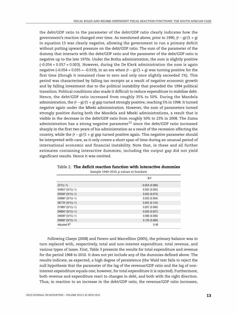
the debt/GDP ratio to the parameter of the debt/GDP ratio clearly indicates how the
government’s reaction changed over time. As mentioned above, prior to 1990, (r – g)/(1 + g)
in equation 13 was clearly negative, allowing the government to run a primary deficit
without putting upward pressure on the debt/GDP ratio. The sum of the parameter of the
dummy that interacts with the debt/GDP ratio and the parameter of the debt/GDP ratio is
negative up to the late 1970s. Under the Botha administration, the sum is slightly positive
(–0.054 + 0.057 = 0.003). However, during the De Klerk administration the sum is again
negative (–0.054 + 0.035 = –0.019), in an era when (r – g)/(1 + g) was turning positive for the
first time (though it remained close to zero and only once slightly exceeded 1%). This
period was characterised by falling tax receipts as a result of negative economic growth
and by falling investment due to the political instability that preceded the 1994 political
transition. Political conditions also made it difficult to reduce expenditure to stabilise debt.
Hence, the debt/GDP ratio increased from roughly 35% to 50%. During the Mandela
administration, the (r – g)/(1 + g) gap turned strongly positive, reaching 5% in 1998. It turned
negative again under the Mbeki administration. However, the sum of parameters turned
strongly positive during both the Mandela and Mbeki administrations, a result that is
visible in the decrease in the debt/GDP ratio from roughly 50% to 23% in 2008. The Zuma
administration has a strong negative parameter12 since the debt/GDP ratio increased
sharply in the first two years of his administration as a result of the recession affecting the
country, while the (r – g)/(1 + g) gap turned positive again. This negative parameter should
be interpreted with care, as it only covers a short span of time during an unusual period of
international economic and financial instability. Note that, in these and all further
estimates containing interactive dummies, including the output gap did not yield
significant results. Hence it was omitted.
Following Claeys (2008) and Favero and Marcellino (2005), the primary balance was in
turn replaced with, respectively, total and non-interest expenditure, total revenue, and
various types of taxes. First, Table 3 presents the results for total expenditure and revenue
for the period 1968 to 2010. It does not yet include any of the dummies defined above. The
results indicate, as expected, a high degree of persistence (the Wald test fails to reject the
null hypothesis that the parameter of the lag of the revenue/GDP ratio and the lag of non-
interest expenditure equals one; however, for total expenditure it is rejected). Furthermore,
both revenue and expenditure react to changes in debt, and both with the right direction.
Thus, in reaction to an increase in the debt/GDP ratio, the revenue/GDP ratio increases,
Table 2. The deficit reaction function with interactive dummiesSample 1949-2010; p values in brackets
B/Y
(D/Y)(–1) –0.054 (0.000)
D4954*(D/Y)(–1) 0.032 (0.002)
D5558*(D/Y)(–1) 0.023 (0.073)
D5966*(D/Y)(–1) 0.033 (0.004)
D6778*(D/Y)(–1) 0.022 (0.152)
D7989*(D/Y)(–1) 0.057 (0.000)
D9094*(D/Y)(–1) 0.035 (0.027)
D9599*(D/Y)(–1) 0.090 (0.000)
D0008*(D/Y)(–1) 0.125 (0.000)
Adjusted R2 0.48
FISCAL RULES AND REGIME-DEPENDENT FISCAL REACTION FUNCTIONS: THE SOUTH AFRICAN CASE
OECD JOURNAL ON BUDGETING – VOLUME 2012/1 © OECD 201214
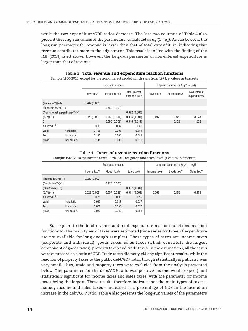
while the two expenditure/GDP ratios decrease. The last two columns of Table 4 also
present the long-run values of the parameters, calculated as α3/(1 – α2). As can be seen, the
long-run parameter for revenue is larger than that of total expenditure, indicating that
revenue contributes more to the adjustment. This result is in line with the finding of the
IMF (2011) cited above. However, the long-run parameter of non-interest expenditure is
larger than that of revenue.
Subsequent to the total revenue and total expenditure reaction functions, reaction
functions for the main types of taxes were estimated (time series for types of expenditure
are not available for long enough samples). These types of taxes are income taxes
(corporate and individual), goods taxes, sales taxes (which constitute the largest
component of goods taxes), property taxes and trade taxes. In the estimations, all the taxes
were expressed as a ratio of GDP. Trade taxes did not yield any significant results, while the
reaction of property taxes to the public debt/GDP ratio, though statistically significant, was
very small. Thus, trade and property taxes were excluded from the analysis presented
below. The parameter for the debt/GDP ratio was positive (as one would expect) and
statistically significant for income taxes and sales taxes, with the parameter for income
taxes being the largest. These results therefore indicate that the main types of taxes –
namely income and sales taxes – increased as a percentage of GDP in the face of an
increase in the debt/GDP ratio. Table 4 also presents the long-run values of the parameters
Table 3. Total revenue and expenditure reaction functionsSample 1960-2010, except for the non-interest model which runs from 1971; p values in brackets
Estimated models Long-run parameters [α3/(1 – α2)]
Revenue/Y Expenditure/YNon-interest
expenditure/YRevenue/Y Expenditure/Y
Non-interest expenditure/Y
(Revenue/Y)(–1) 0.967 (0.000)
(Expenditure/Y)(–1) 0.860 (0.000)
(Non-interest expenditure/Y)(–1) 0.972 (0.000)
(D/Y)(–1) 0.023 (0.039) –0.060 (0.014) –0.095 (0.001) 0.697 –0.429 –3.373
C 0.060 (0.003) 0.045 (0.013) 0.429 1.602
Adjusted R2 0.93 0.87 0.89
Wald t-statistic 0.155 0.006 0.681
Test F-statistic 0.155 0.006 0.681
(Prob) Chi-square 0.148 0.006 0.679
Table 4. Types of revenue reaction functionsSample 1968-2010 for income taxes; 1970-2010 for goods and sales taxes; p values in brackets
Estimated models Long-run parameters [α3/(1 – α2)]
Income tax/Y Goods tax/Y Sales tax/Y Income tax/Y Goods tax/Y Sales tax/Y
(Income tax/Y)(–1) 0.923 (0.000)
(Goods tax/Y)(–1) 0.976 (0.000)
(Sales tax/Y)(–1) 0.937 (0.000)
(D/Y)(–1) 0.028 (0.009) 0.007 (0.222) 0.011 (0.008) 0.363 0.156 0.173
Adjusted R2 0.78 0.96 0.95
Wald t-statistic 0.029 0.388 0.027
Test F-statistic 0.029 0.388 0.027
(Prob) Chi-square 0.023 0.383 0.021
FISCAL RULES AND REGIME-DEPENDENT FISCAL REACTION FUNCTIONS: THE SOUTH AFRICAN CASE
OECD JOURNAL ON BUDGETING – VOLUME 2012/1 © OECD 2012 15
from which it is clear that, in the income tax/GDP ratio equation, the long-run parameter
value for the debt/GDP ratio is the largest.
The estimates containing the interactive dummies for the terms of administration of
the various prime ministers and presidents yield significant results (presented for the
period 1960-2010; see Table 5). Note that the parameter for the debt/GDP ratio itself was
statistically insignificantly different from zero (thus indicating no reaction in the Zuma
administration – again a result that should be considered with caution since the
administration is young and took power during a recession, so the administration has not
had the opportunity to demonstrate fully its stance with regard to debt). Therefore, the
reaction of each administration is summarised by the parameter for the interactive
dummy multiplied by the debt/GDP ratio. Table 5 shows that both revenue and expenditure
consistently reacted to increases in debt with the requisite sign (positive for revenue and
negative for expenditure). It should also be noted that, once one controls for the different
regimes, the Wald test – conducted to determine whether the parameters on the lags of the
revenue/GDP and expenditure/GDP ratios equal one – is rejected. Lastly, Table 5 also
presents the long-run values of the parameters from which it is clear that, in the revenue/
GDP ratio equation, the long-run parameter value for the debt/GDP ratio is larger than in
both the expenditure/GDP ratio and the non-interest expenditure/GDP ratio equations.
Thus, the finding that the non-interest expenditure/GDP ratio responds with more than
the revenue found when the regression was run without the interactive dummies is
overturned when including the interactive dummies.
Table 6 presents regressions with the income tax/GDP ratio, the goods tax/GDP ratio
and the sales tax/GDP ratio. The income tax/GDP ratio was regressed on its own lag and the
dummies for the terms of prime ministers and presidents that interact with the public
debt/GDP ratio. Note that the debt/GDP ratio is not included, as it is statistically
insignificant when included. The parameters show a consistent reaction of the income tax/
GDP ratio, with the lowest reactions in the period 1989-94 (a period of low growth and thus
lower tax income due to the political uncertainty preceding the transition to democracy)
and, of course, the period 2009-10 when the parameter has a zero value (as indicated by the
debt/GDP ratio being omitted from the model due to its statistical insignificance). The Wald
test also indicates that the parameter on the lagged value of the income tax/GDP ratio is
not equal to one.
Table 6 also presents estimates for the goods tax/GDP and sales tax/GDP ratios. As
mentioned above, sales tax constitutes the largest proportion of goods taxes, with the
petrol levy being the second-largest component. Estimations with the terms of the various
prime ministers did not yield satisfactory results. A possible explanation for this might be
the rather fragmented history of sales tax. In 1970, the government imposed a sales tax on
goods when the goods left the factory or were imported. According to Browne (1983), this
sales tax did not yield the expected income stream for the government. Therefore, the
government replaced this first sales tax in 1978 with the general sales tax (GST) levied on
final consumers at a rate of 4%. In 1991, the government in turn replaced the GST – then
levied at 12% – with the value-added tax (VAT) at a rate of 10%. Thereafter the VAT rate
increased to 14% (the debt burden also increased during the same period).13 Since the ANC
government came to power, it has not changed the VAT rate.
Therefore, instead of using the terms of prime ministers and presidents, dummy
variables that respectively cover the GST period (1978-90) and the VAT period (1991-2010)

FISCAL RULES AND REGIME-DEPENDENT FISCAL REACTION FUNCTIONS: THE SOUTH AFRICAN CASE
OECD JOURNAL ON BUDGETING – VOLUME 2012/1 © OECD 201216
were created and subsequently interacted with the debt/GDP ratio. Table 6 shows that both
these dummy variables interacting with the debt/GDP ratio have the correct sign and are
statistically significant. The positive value for the VAT dummy interacting with the debt/
GDP ratio in the face of an unchanged VAT rate since the mid-1990s possibly follows from
the sharp increase in the VAT rate in the early 1990s, during a period in which the debt/GDP
ratio also increased sharply.
To conclude, the above discussion shows that, once one controls for different
administrations or changes made to the types of taxes levied, as was the case with GST and
VAT, almost all the series turned out to be stationary – a finding that concurs with the
Table 5. Total revenue and expenditure reaction functionswith interactive dummies
Sample 1960-2010, except for the non-interest model which runs from 1971; p values in brackets
Estimated models Long-run parameters [α3/(1 – α2)]
Revenue/Y Expenditure/YNon-interest
expenditure/YRevenue/Y Expenditure/Y
Non-interest expenditure/Y
(Revenue/Y)(–1) 0.961 (0.000)
(Expenditure/Y)(–1) 0.573 (0.006)
(Non-interest expenditure/Y)(–1) 0.548 (0.009)
D5966*(D/Y)(–1) 0.019 (0.011) –0.120 (0.023) 0.499 –0.282
D6778*(D/Y)(–1) 0.025 (0.002) –0.094 (0.009) –0.148 (0.009) 0.642 –0.220 –0.327
D7989*(D/Y)(–1) 0.035 (0.006) –0.089 (0.027) –0.125 (0.006) 0.897 –0.209 –0.277
D9094*(D/Y)(–1) 0.017 (0.173) –0.052 (0.015) –0.057 (0.020) 0.429 –0.122 –0.127
D9599*(D/Y)(–1) 0.025 (0.001) –0.043 (0.012) –0.061 (0.002) 0.647 –0.100 –0.135
D0008*(D/Y)(–1) 0.024 (0.125) –0.071 (0.007) –0.076 (0.002) 0.622 –0.166 –0.168
C 0.136 (0.021) 0.140 (0.009) 0.318 0.309
Adjusted R2 0.92 0.87 0.86
Wald t-statistic 0.018 0.036 0.029
Test F-statistic 0.018 0.036 0.029
(Prob) Chi-square 0.014 0.030 0.022
Table 6. Types of revenue reaction functions with interactive dummiesp values in brackets
Estimated models Long-run parameters [α3/(1 – α2)]
Income tax/Y1 Goods tax/Y2 Sales tax/Y2 Income tax/Y1 Goods tax/Y2 Sales tax/Y2
(Income tax/Y)(–1) 0.943 (0.000)
(Goods tax/Y)(–1) 0.968 (0.000)
(Sales tax/Y)(–1) 0.935 (0.000)
D7890*(D/Y)(–1) 0.018 (0.000) 0.019 (0.000) 0.563 0.292
D9110*(D/Y)(–1) 0.006 (0.035) 0.011 (0.011) 0.188 0.169
D6778*(D/Y)(–1) 0.028 (0.000) 0.485
D7989*(D/Y)(–1) 0.024 (0.000) 0.416
D9094*(D/Y)(–1) 0.011 (0.157) 0.195
D9599*(D/Y)(–1) 0.020 (0.000) 0.353
D0008*(D/Y)(–1) 0.024 (0.014) 0.425
Adjusted R2 0.78 0.97 0.97
Wald t-statistic 0.000 0.006 0.024
Test F-statistic 0.000 0.006 0.024
(Prob) Chi-square 0.000 0.003 0.018
1. Sample 1968-2010.2. Sample 1970-2010.

FISCAL RULES AND REGIME-DEPENDENT FISCAL REACTION FUNCTIONS: THE SOUTH AFRICAN CASE
OECD JOURNAL ON BUDGETING – VOLUME 2012/1 © OECD 2012 17
arguments of Bohn, Claeys, and Favero and Marcellino that these series are inherently
stationary.
More importantly, regarding the question raised above as to whether the government
depended on adjustments to revenues or expenditures – or both – when pursuing a fiscal
rule, the above analysis indicates that when the debt/GDP ratio increased, both revenue
and expenditure adjusted, thereby ensuring the sustainability of fiscal policy in the post-
WWII period. However, when comparing the size of the long-run tax and expenditure
parameters, calculated as α3/(1 – α2), it would appear that the expenditure parameters are
smaller than the tax parameters. This finding accords with the IMF finding about the
behaviour of G7 country governments (IMF, 2011).
Lastly, irrespective of which set of dummies (political administrations or types of sales
taxes) is included in the regressions with the primary balance as dependent variable, it is
clear that the size of the parameters mostly reflects the stance of the (r – g)/(1 + g) gap.
Thus, although the reaction of the various administrations differed, the extent to which
they differed seems to reflect the stance of the (r – g)/(1 + g) gap at the time. Hence, this
analysis calls for the use of a time-varying analysis that controls for the movements in the
(r – g)/(1 + g) gap. This is done in subsection 4.4 below.
4.3. Allowing for a time-varying reaction to the debt/GDP ratio usinga Markov-switching model
Using quarterly data for the period 1972Q1-2010Q4 (i.e. 156 observations), this section
presents the Markov-switching estimations for fiscal reaction functions as specified in
equations 13 and 16. Because of a lack of data, the analysis does not attempt to extend its
examination to the period prior to the 1970s. Thus, the analysis uses the primary balance
calculated with government data. The following two specifications were estimated for
South Africa over the period:
(B/Y)tActual = α0st + α1st(B/Y)t-4
Actual + α2styt-4 + α3st(D/Y)t-4 + εtst (13.1)
(B/Y)tActual = β0st + β1st(B/Y)t-4 Actual + β2styt-4 + γ1st(B/Y)Required
t-4 + υtst (16.1)
where subscript s is a state variable that is unobserved and assumed to be generated by a
probability distribution that takes into account both the parameters and the variables in
the model. In addition, s takes on values of N = 1, 2, thus denoting two regimes (i.e. the
assumption of a two-state Markov chain is made). Transition probabilities are given by
pij = Pr(st = j| st-1 = i) and, assuming that the current regime is i, the expected average
duration of staying in the same regime is (1 – pii)-1. The specification in equations 13.1
and 16.1 allows all of the model parameters to vary across regimes. Lastly, errors εt and υt
are considered to be normally distributed with a zero mean and a constant variance that is
allowed to be different in each regime.14 Note that all of the regressors have been lagged
four quarters to capture the annual nature of the national budget process. Tables 7 and 8
below report the estimation results.
The bottom row in Table 7 reports the results obtained making the assumption of a
constant fiscal regime over the estimation period. This model uses the same data as the
model reported in Table 1, the only difference being that Table 1 uses an annual frequency,
while Table 7 is quarterly. The parameters are statistically significant and indicate that
fiscal policy has been active and pro-cyclical over the estimation sample. With respect to
the Markov-switching model, the results reported in Table 7 show that two fiscal regimes
can be identified for South Africa over the estimation sample. Regime 1 has a positive and

FISCAL RULES AND REGIME-DEPENDENT FISCAL REACTION FUNCTIONS: THE SOUTH AFRICAN CASE
OECD JOURNAL ON BUDGETING – VOLUME 2012/1 © OECD 201218
statistically significant α3 coefficient (i.e. fiscal pacifism) and a negative (i.e. pro-cyclical)
and statistically significant α2 coefficient. Regime 2 has a positive and statistically
insignificant α3 coefficient (i.e. fiscal activism) and a positive (i.e. counter-cyclical) and
statistically significant α3 coefficient. In terms of the durations of the two regimes,
Regime 1 is more persistent, with Regime 2 detected in three brief periods: 1980-82, 1992-94
and 2009-10 (see Figure 2 that indicates the probability of being in Regime 1). Notice that
especially the last two periods were characterised by relatively sharp increases in the debt/
GDP ratio (while in the case of the first period, it marked the end of the longer-run decrease
in the debt/GDP ratio).
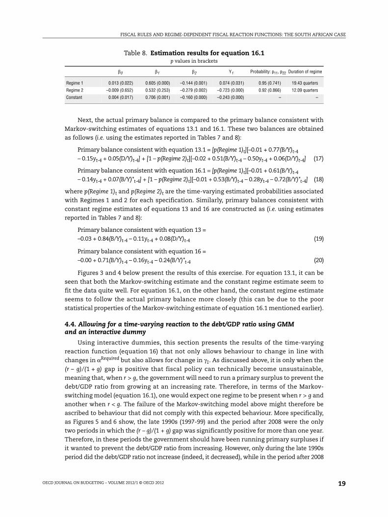
The estimates under the assumption of a constant regime, reported in the bottom row
of Table 8, indicate that fiscal policy in South Africa has been active and pro-cyclical.
However, these results imply that, when r > g, the government did not run a sustainable
fiscal policy by adjusting the size of the actual primary balance to fit the size of the
required primary balance. This contradicts the results in Table 7. The results of the
estimation for equation 16.1 are also reported in Table 8. Equation 16.1 explores the
possibility that γ1 is also a time-varying parameter (in addition to αRequired in equation 16).
While the majority of the coefficients are statistically significant, the transition probability
estimates are not and thus cast doubt on the time-varying probabilities associated with the
assumed two regimes.
Table 7. Estimation results for equation 13.1p values in brackets
α0 α1 α2 α3 Probability: p11, p22 Duration of regime
Regime 1 –0.012 (0.013) 0.765 (0.000) –0.150 (0.000) 0.052 (0.000) 0.97 (0.000) 32.67 quarters
Regime 2 –0.027 (0.341) 0.506 (0.177) 0.495 (0.000) 0.059 (0.201) 0.84 (0.000) 6.37 quarters
Constant –0.027 (0.001) 0.836 (0.000) –0.115 (0.012) 0.083 (0.000) – –
Figure 2. The probability of being in Regime 1
Source: Authors’ own calculations using data from the South African Reserve Bank.
1.1
1.0
0.9
0.8
0.7
0.6
0.5
0.4
0.3
0.2
0.1
0
Equation 13.1 – Markov-switching(2) model
1972
Q1
1974
Q1
1976
Q1
1978
Q1
1980
Q1
1982
Q1
1984
Q1
1986
Q1
1988
Q1
1990
Q1
1992
Q1
1994
Q1
1996
Q1
1998
Q1
2000
Q1
2002
Q1
2004
Q1
2006
Q1
2008
Q1
2010
Q1
FISCAL RULES AND REGIME-DEPENDENT FISCAL REACTION FUNCTIONS: THE SOUTH AFRICAN CASE
OECD JOURNAL ON BUDGETING – VOLUME 2012/1 © OECD 2012 19
Next, the actual primary balance is compared to the primary balance consistent with
Markov-switching estimates of equations 13.1 and 16.1. These two balances are obtained
as follows (i.e. using the estimates reported in Tables 7 and 8):
Primary balance consistent with equation 13.1 = [p(Regime 1)t][–0.01 + 0.77(B/Y)t-4
– 0.15yt-4 + 0.05(D/Y)t-4] + [1 – p(Regime 2)t][–0.02 + 0.51(B/Y)t-4 – 0.50yt-4 + 0.06(D/Y)t-4] (17)
Primary balance consistent with equation 16.1 = [p(Regime 1)t][–0.01 + 0.61(B/Y)t-4
– 0.14yt-4 + 0.07(B/Y)*t-4] + [1 – p(Regime 2)t][–0.01 + 0.53(B/Y)t-4 – 0.28yt-4 – 0.72(B/Y)*t-4] (18)
where p(Regime 1)t and p(Regime 2)t are the time-varying estimated probabilities associated
with Regimes 1 and 2 for each specification. Similarly, primary balances consistent with
constant regime estimates of equations 13 and 16 are constructed as (i.e. using estimates
reported in Tables 7 and 8):
Primary balance consistent with equation 13 =
–0.03 + 0.84(B/Y)t-4 – 0.11yt-4 + 0.08(D/Y)t-4 (19)
Primary balance consistent with equation 16 =
–0.00 + 0.71(B/Y)t-4 – 0.16yt-4 – 0.24(B/Y)*t-4 (20)
Figures 3 and 4 below present the results of this exercise. For equation 13.1, it can be
seen that both the Markov-switching estimate and the constant regime estimate seem to
fit the data quite well. For equation 16.1, on the other hand, the constant regime estimate
seems to follow the actual primary balance more closely (this can be due to the poor
statistical properties of the Markov-switching estimate of equation 16.1 mentioned earlier).
4.4. Allowing for a time-varying reaction to the debt/GDP ratio using GMM and an interactive dummy
Using interactive dummies, this section presents the results of the time-varying
reaction function (equation 16) that not only allows behaviour to change in line with
changes in αRequired but also allows for change in γ1. As discussed above, it is only when the
(r – g)/(1 + g) gap is positive that fiscal policy can technically become unsustainable,
meaning that, when r > g, the government will need to run a primary surplus to prevent the
debt/GDP ratio from growing at an increasing rate. Therefore, in terms of the Markov-
switching model (equation 16.1), one would expect one regime to be present when r > g and
another when r < g. The failure of the Markov-switching model above might therefore be
ascribed to behaviour that did not comply with this expected behaviour. More specifically,
as Figures 5 and 6 show, the late 1990s (1997-99) and the period after 2008 were the only
two periods in which the (r – g)/(1 + g) gap was significantly positive for more than one year.
Therefore, in these periods the government should have been running primary surpluses if
it wanted to prevent the debt/GDP ratio from increasing. However, only during the late 1990s
period did the debt/GDP ratio not increase (indeed, it decreased), while in the period after 2008
Table 8. Estimation results for equation 16.1p values in brackets
β0 β1 β2 Y1 Probability: p11, p22 Duration of regime
Regime 1 0.013 (0.022) 0.605 (0.000) –0.144 (0.001) 0.074 (0.031) 0.95 (0.741) 19.43 quarters
Regime 2 –0.009 (0.652) 0.532 (0.253) –0.279 (0.002) –0.723 (0.000) 0.92 (0.866) 12.09 quarters
Constant 0.004 (0.017) 0.706 (0.001) –0.160 (0.000) –0.243 (0.000) – –

FISCAL RULES AND REGIME-DEPENDENT FISCAL REACTION FUNCTIONS: THE SOUTH AFRICAN CASE
OECD JOURNAL ON BUDGETING – VOLUME 2012/1 © OECD 201220
it did increase. To deal with these two very different reactions to a positive (r – g)/(1 + g) gap,
the analysis created dummies for the two periods that interacted with the required
primary balance. Only the dummy for the period 1997-99 yielded statistically significant
results (presented below). In addition, since the required primary balance is calculated
with the actual effective interest rate of the government obtained from government data,
the actual primary balance measure used is the one calculated with government data.
Table 9 shows that, for most of the sample period, the reaction of the actual primary
balance/GDP ratio to changes in the required primary balance has been negative, only
Figure 3. Comparison of the actual primary balance and the primary balance consistent with equations 13 and 13.1
Source: Authors’ own calculations using data from the South African Reserve Bank.
Figure 4. Comparison of the actual primary balance and the primary balance consistent with equations 16 and 16.1
Source: Authors’ own calculations using data from the South African Reserve Bank.
0.10
0.08
0.06
0.04
0.02
0
-0.02
-0.04
0.10
0.08
0.06
0.04
0
0.02
-0.02
-0.04
Primary balance consistent with(1) (Markov-switching)Primary balance
Primary balance consistent with(1) (Constant regime)Primary balance
1972
Q1
1973
Q3
1975
Q1
1976
Q3
1978
Q1
1979
Q3
1981
Q1
1982
Q3
1984
Q1
1985
Q3
1987
Q1
1988
Q3
1990
Q1
1991
Q3
1993
Q1
1994
Q3
1996
Q1
1997
Q3
1999
Q1
2000
Q3
2002
Q1
2003
Q3
2005
Q1
2006
Q3
2008
Q1
2009
Q3
1972
Q1
1973
Q3
1975
Q1
1976
Q3
1978
Q1
1979
Q3
1981
Q1
1982
Q3
1984
Q1
1985
Q3
1987
Q1
1988
Q3
1990
Q1
1991
Q3
1993
Q1
1994
Q3
1996
Q1
1997
Q3
1999
Q1
2000
Q3
2002
Q1
2003
Q3
2005
Q1
2006
Q3
2008
Q1
2009
Q3
0.10
0.08
0.06
0.04
0.02
0
-0.02
-0.04
0.10
0.08
0.06
0.04
0
0.02
-0.02
-0.04
Primary balance consistent with(2) (Markov-switching)Primary balance
Primary balance consistent with(2) (Constant regime)Primary balance
1972
Q1
1973
Q3
1975
Q1
1976
Q3
1978
Q1
1979
Q3
1981
Q1
1982
Q3
1984
Q1
1985
Q3
1987
Q1
1988
Q3
1990
Q1
1991
Q3
1993
Q1
1994
Q3
1996
Q1
1997
Q3
1999
Q1
2000
Q3
2002
Q1
2003
Q3
2005
Q1
2006
Q3
2008
Q1
2009
Q3
1972
Q1
1973
Q3
1975
Q1
1976
Q3
1978
Q1
1979
Q3
1981
Q1
1982
Q3
1984
Q1
1985
Q3
1987
Q1
1988
Q3
1990
Q1
1991
Q3
1993
Q1
1994
Q3
1996
Q1
1997
Q3
1999
Q1
2000
Q3
2002
Q1
2003
Q3
2005
Q1
2006
Q3
2008
Q1
2009
Q3

FISCAL RULES AND REGIME-DEPENDENT FISCAL REACTION FUNCTIONS: THE SOUTH AFRICAN CASE
OECD JOURNAL ON BUDGETING – VOLUME 2012/1 © OECD 2012 21
turning positive for the period 1997-99. As mentioned above, when the (r – g)/(1 + g) gap is
positive, the primary balance should increase in response to an increase in the required
primary balance. The government’s behaviour accorded with this requirement in the late
1990s, but not in the period since 2008. As discussed above, when the (r – g)/(1 + g) gap is
positive, the value for the parameter of the required primary balance/GDP ratio is expected
to equal 1. The Wald test indicates that the null hypothesis (that α2 + α3 = 1) cannot be
rejected, pointing to the government acting in a fiscally sustainable manner during the
budgets for the period 1997-99.
When the (r – g)/(1 + g) gap is negative, the government can run a primary deficit
without putting upward pressure on the debt/GDP ratio. Should it run a larger primary
deficit than is required to keep the debt/GDP ratio stable, the debt/GDP ratio will increase
but at a decreasing rate, thus converging to a higher level – i.e. it will not display explosive
behaviour.15 Thus, for periods when the (r – g)/(1 + g) gap is negative, one would expect the
parameter for the required primary balance to be statistically insignificant, or negative and
Figure 5. The (r – g)/(1 + g) relationship
Source: South African Reserve Bank and authors’ own calculations.
Figure 6. The (r – g)/(1 + g) gap and the actual and required primary balances
Source: South African Reserve Bank and authors’ own calculations.
0.35
0.30
0.25
0.20
0.15
0.10
0.05
0
-0.05
-0.10
-0.15
-0.201971 1973 1975 1977 1979 1981 1983 1985 1987 1989 1991 1993 1995 1997 1999 2001 2003 2005 2007 2009
Nominal GDP growth Nominal effective interest rate (r – g)/(1 + g)
0.08
0.06
0.04
0.02
0
-0.02
-0.04
-0.06
-0.081971 1973 1975 1977 1979 1981 1983 1985 1987 1989 1991 1993 1995 1997 1999 2001 2003 2005 2007 2009
(r – g)/(1 + g) > 0 Actual primary balance/GDP ratio Required primary balance/GDP ratio

FISCAL RULES AND REGIME-DEPENDENT FISCAL REACTION FUNCTIONS: THE SOUTH AFRICAN CASE
OECD JOURNAL ON BUDGETING – VOLUME 2012/1 © OECD 201222
statistically significant, indicating a government that pursued a counter-cyclical fiscal
policy.16 As indicated by the negative parameter for the required primary balance in times
when the (r – g)/(1 + g) gap was negative, this counter-cyclical fiscal policy seems to have
been present in South Africa particularly when the (r – g)/(1 + g) gap was negative (also see
Figures 5 and 6). Furthermore, given the statistical insignificance of the dummy for the
short period after 2008 (and hence its exclusion from the model), counter-cyclical policy
might also have dominated the requirement to stabilise the debt/GDP ratio even though
the (r – g)/(1 + g) gap was positive. However, what seems to contrast with the counter-
cyclical behaviour of the actual primary balance with respect to movements in the required
primary balance (i.e. the negative parameter on the required primary balance) is the pro-
cyclical impact of the output gap (i.e. the negative parameter of the output gap).
Table 9 also presents the results for the reaction function estimated with expenditure
and revenue. Revenue seems to always move in the same direction as the required primary
surplus, with a positive parameter of 0.222. However, both total and non-interest
expenditure seem to move counter-cyclically when the (r – g)/(1 + g) gap is negative.
Nevertheless, as can be seen from adding the parameter on the required primary balance
to that of the required primary balance multiplied by the interactive dummy, both total and
non-interest expenditure act to stabilise the actual primary balance by decreasing when
the required primary balance increases. In addition, as can be expected given that interest
expenditure is non-discretionary, the parameters in the non-interest expenditure model
are larger than those in the total expenditure model. Comparing the behaviour of the
different models shows that expenditure displays the same behaviour as the primary
balance. Re-specifying the models with the different types of taxes did not yield good
results, indicating that the behaviour of revenue is mostly displayed on the aggregate level
and not so much on the level of individual types of revenue. In addition, the output gap was
not significant in any of the expenditure or revenue models; hence it was excluded from
the final specification.
4.5. Explaining the results
If – following Bohn, Claeys, Favero and Marcellino, and Favero and Monacelli – the
primary balance/GDP and debt/GDP ratios are taken as stationary, one can then follow
Table 9. Reaction functions with time-varying debt parametersSample 1971-2010; p values in brackets
B/Y1 Revenue/Y Expenditure/Y Non-interest expenditure/Y
(B/Y)(–1) 0.720 (0.000)
(Revenue/Y)(–1) 0.840 (0.000)
(Expenditure/Y)(–1) 0.676 (0.005)
(Non-interest expenditure/Y)(–1) 0.450 (0.006)
(B/Y)Required –0.484 (0.034) 0.222 (0.055) 0.242 (0.288) 1.146 (0.002)
D9799*(B/Y)Required 1.470 (0.000) –0.520 (0.045) –1.377 (0.002)
Y gap(–1) –0.422 (0.032)
C 0.037 (0.010) 0.087 (0.146) 0.138 (0.001)
Adjusted R2 0.21 0.82 0.70 0.78
Wald t-statistic 0.909
Test F-statistic 0.909
(Prob) Chi-square 0.909
1. Wald test H0: α2 + α3 = 1.

FISCAL RULES AND REGIME-DEPENDENT FISCAL REACTION FUNCTIONS: THE SOUTH AFRICAN CASE
OECD JOURNAL ON BUDGETING – VOLUME 2012/1 © OECD 2012 23
these authors further by estimating fiscal reaction functions. Indeed, when estimating
these reaction functions and controlling for changing behaviour over time, the persistence
parameters in these relationships are less than one, whether the relationship is estimated
with GMM or a Markov-switching model. In GMM models where the parameters were close
to but less than one, the Wald tests indicate that they nevertheless are statistically
significantly less than one.
In the reaction functions containing the debt/GDP ratio, the inclusion of interactive
dummies multiplied by the debt/GDP ratio indicates that:
● The behaviour of total and non-interest expenditure as well as the different types of
revenue changed over time.
● The size of the reaction of the primary balance to changes in the debt/GDP ratio mostly
seems to reflect the stance of the (r – g)/(1 + g) gap.
● The reaction of the revenue/GDP ratio to changes in the debt/GDP ratio is larger than that
of the expenditure/GDP ratio. This is in accordance with recent findings by the IMF for
the G7 countries (IMF, 2011).
Table 10 contains the summary of the different models estimated in subsections 4.1
through 4.4. The first row reports the signs of the (r – g)/(1 + g) gap over the period 1971-
2010. Subsequent rows report the government’s reaction to an increase in public debt (in
the case of the baseline model as well as models 1 and 2) or to an increase in the required
primary balance (in the case of model 3). Given that model 3 regresses the actual budget
balance on the required budget balance, the sign of the (r – g)/(1 + g) gap needs to be taken
into account when interpreting the coefficient estimates. This has been done in the last
row of Table 10 where the signs of the estimated coefficients γ1αRequired change when the
(r – g)/(1 + g) gap is negative (i.e. when fiscal policy can technically not become
unsustainable). What is notable is the relatively high degree of consistency in terms of the
results, particularly when considering that different frequencies of the data (quarterly and
annual) as well as different estimation techniques were used (GMM with dummy variables
that impose exogenously determined regimes and Markov-switching estimations where
the regimes are endogenously determined). The baseline model indicates that the
government has been fiscally passive (indicated by white cells) over the entire sample
under consideration, whereas models 1-3 indicate that the government has been largely
fiscally passive over the same sample period. Episodes where models 1-3 indicate fiscal
activism (indicated by darker cells) and no (or ambiguous) government reaction (indicated
by lighter cells) are also consistent for the most part – particularly for the periods 1990-94
and 2008-10. It should be noted that the fiscal activism indicated during the 2008-10 period
makes a case for fiscal guidelines (or fiscal rules) given that debt levels are rising and that
there are some real pressures on the budget (such as job-creation efforts set out in the New
Growth Path as well as the National Health Insurance).
According to the estimates of equations 13, 13.1, 16 and 16.1 that contain an output
gap, the reaction of the actual primary balance to the output gap is pro-cyclical. However,
it should also be mentioned that the inclusion of the political administration dummies
rendered the output gap statistically insignificant. It is also insignificant in the expenditure
and revenue models controlling for the (r – g)/(1 + g) gap (i.e. the expenditure and revenue
versions of equation 16). The analysis also shows that, when the (r – g)/(1 + g) gap was
positive in the period 1997-99, the government did act to contain debt and ensure fiscal
sustainability. More specifically, the analysis shows that the actual primary balance

FISCAL RULES AND REGIME-DEPENDENT FISCAL REACTION FUNCTIONS: THE SOUTH AFRICAN CASE
OECD JOURNAL ON BUDGETING – VOLUME 2012/1 © OECD 201224
reacted to the size of the required primary balance to the extent that the public debt/GDP
ratio did not increase during that period. However, the same cannot be said for the period
after 2008.
5. Adjusting the sensitivity of the automatic stabilisersThe estimations above indicate that the reaction of the revenue/GDP ratio to the debt/
GDP ratio is larger than that of the expenditure/GDP ratio. Thus, there might be a need to
enhance the reaction of the expenditure/GDP ratio. In addition, the fiscal rule set out above
allows for the deficit to move in a counter-cyclical fashion by allowing revenue to drop and
expenditure to increase when the economy experiences a recession. With government
expenditure and revenue set to vary around a predefined long-run level, the rule very much
depends on the workings of the automatic stabilisers. The government’s reaction to the
cycle is therefore “automated”. However, as the reaction of many countries to the 2008/09
financial crisis indicated, governments also change their discretionary fiscal policy. This of
course raises the question as to whether or not the burden of reaction should not be shifted
to a larger extent to the automatic stabilisers, thereby automating fiscal reaction much
more. Automatic stabilisers eliminate the observation and decision lags that hamper
discretionary reactions. Shifting the burden of reaction more to the automatic stabilisers,
though, may require the enhancement of these stabilisers.
Baunsgaard and Symansky (2009) suggested several ways in which the automatic
stabilisers can be enhanced without increasing the size of government. These include
permanent and temporary changes to tax and expenditure frameworks. Temporary
changes are like trip-switches that are triggered when specific macroeconomic thresholds
are crossed (Baunsgaard and Symansky, 2009:6). Baunsgaard and Symansky (2009:8-11)
argue that changes to permanent measures, such as increasing the progressiveness of
personal income tax or increasing the share of personal income tax in total revenues
collected, will not yield a significant enhancement of the automatic stabilisers. Thus, they
argue for the use of temporary measures.
Baunsgaard and Symansky (2009:16-17) thus propose the use of temporary measures
with high multiplier effects such as temporary tax policies targeted at low-income
households that are probably credit or liquidity constrained. These measures could take
Table 10. Summary of the estimation results: reaction of the primary balance to either debt (models 1 and 2) or the required primary balance (model 3)1
Sign of the(r – g)/(1 + g)
gap
1971-90(–)
1991-96(0)
1997-99(+)
2000-08(+/–)
2009-2010(+)
Reaction of the government
Baseline model 1971-2010 (+)
Model 1 1971-78 (–) 1979-89 (+) 1990-94 (–) 1995-2008 (+) 2009-10 (–)
Model 2 1972-81 (+) 1981-82 (0) 1982-90 (+) 1990-94 (0) 1994-2009 (+) 2009-10 (0)
Model 3 1971-90(–)(–) = (+)
1991-96(–)(0) = (0)
1997-99(+)(+) = (+)
2000-08(–)(+/–) = (–/+)
2009-10(–)(+) = (–)
1. The baseline model and model 1 are reported in Table 3 and Table 4, respectively (subsection 4.2 above). Model 2 is theMarkov-switching model reported in Table 7 (subsection 4.3 above), while model 3 is reported in the second column ofTable 9 (subsection 4.4 above). For model 3, note that the first sign in brackets each time represents the sign of theparameter (i.e. the reaction of the primary balance to the required primary balance), while the second sign represents thesign of the (r – g)/(1 + g) gap. Thus, the sign in brackets on the right-hand side of the equal sign represents their combinedsign and thus the sign of the reaction of the primary balance to debt (γ1αRequired).

FISCAL RULES AND REGIME-DEPENDENT FISCAL REACTION FUNCTIONS: THE SOUTH AFRICAN CASE
OECD JOURNAL ON BUDGETING – VOLUME 2012/1 © OECD 2012 25
the form of rebates on personal income taxes, temporary reductions in VAT, temporary
investment tax incentives for businesses that might be credit or liquidity constrained, and
temporary tax credits for job creation. On the expenditure side, the government could use
temporary transfers, again to credit and liquidity constrained households, as well as
temporarily expand existing unemployment benefits (e.g. longer period of eligibility, higher
benefits). Furthermore, transfers to lower levels of government will alleviate the pressure
on lower tiers of government when these are not allowed to run budget deficits
(Baunsgaard and Symansky, 2009:17).
In addition to the measures listed by Baunsgaard and Symansky (2009), the
government could also create a catalogue of “shovel-ready infrastructure projects”.
Usually, investment projects do not make for good fiscal stimulus projects. In addition to
the observation and decision lags that hamper all discretionary fiscal policy, infrastructure
projects also suffer from a long implementation phase. Project specifications must be
drawn up and a tender process then followed which, in turn, is followed by contractual
negotiations. However, the government could have a catalogue of projects that are already
negotiated and concluded with private construction companies that are activated once a
recession occurs. Such a catalogue can be modelled on the United Kingdom Strategic
Infrastructure Partnership model (SIP). This model is ideal when there are successive
phases of similar types of work. In such a model there is certainty about the kind of
infrastructure, but there is uncertainty with regard to the timing and exact phases of the
work (cf. HM Treasury, 2008:21-22).17 Another measure to use with a trip-switch would be
the payment of temporary subsidies to employers not to retrench workers. Thus, the
government pays companies directly to keep workers employed. This also means that
companies do not lose good workers and are geared to benefit from the upswing the
moment conditions improve.
The implementation of temporary measures needs to depend on economic trigger
indicators (or trip-switches). Only when the indicator reaches a particular value will the
measure be activated. In addition, the trigger also needs to work in the opposite direction,
so as to ensure the deactivation of the temporary measure. This will provide an automatic
“exit strategy” from such a stimulus policy. GDP, which is usually only available with a lag,
might not be the most suitable indicator. More timely data or forward-looking indicators
would make for better indicators. Baunsgaard and Symansky (2009:16) mention Feldstein’s
2007 proposal for the United States to use a three-month cumulative decline in payroll
employment as a trigger point, and Elmendorf and Furman’s 2008 proposal for a three-
month change in employment that is negative for three successive months. Forward-
looking indicators require proper forecasting, and Baunsgaard and Symansky (2009:16)
suggest that this be done by an independent agency to prevent manipulation by the
government and to ensure credibility.
6. ConclusionThis article contains a proposal for the use of a simple deficit-and-debt fiscal rule.
Because of the difficulty of forecasting deficits and macroeconomic variables such as
output and potential output with a satisfactory degree of precision, the fiscal framework
contained in this article proposes a permanent (fiscal rule) target that targets the standard
deviation of the deficit instead of the level of budget deficit. Using historic data about the
output gap, as well as estimates of tax and expenditure elasticities, a government can set
a band around the structural budget balance within which the actual deficit will be allowed

FISCAL RULES AND REGIME-DEPENDENT FISCAL REACTION FUNCTIONS: THE SOUTH AFRICAN CASE
OECD JOURNAL ON BUDGETING – VOLUME 2012/1 © OECD 201226
to fluctuate. The government then needs to ensure that the deficit budgeted for the next
year falls within the band. Setting the deficit within a band then allows the automatic
stabilisers to act. As discussed, the benefit of this approach is that when the actual deficit
then deviates from the budgeted deficit, the probability is high that the actual deficit still
falls within the target band. The government is then guided by the fiscal rule but, where
deviations still fall within the target band, it will not lose credibility when the actual deficit
deviates from the budgeted deficit.
The estimates of the fiscal reaction function showed that, historically, the South
African government contained debt and ensured fiscal sustainability. Thus, in general the
South African government ran a passive fiscal policy. The exceptions were the early 1990s
and the period since 2008, periods during which the debt burden increased. The fiscal
activism observed during the 2008-10 period makes a case for fiscal guidelines (or fiscal
rules) given that debt levels are rising and that there are some real pressures on the budget
(such as job-creation efforts set out in the New Growth Path as well as the National Health
Insurance).
Compared to the expenditure/GDP ratio, the revenue/GDP ratio was historically more
reactive to changes in the debt/GDP ratio. This is in line with behaviour in G7 countries.
The government could also consider measures to increase this reactiveness of revenue and
expenditure, both to changes in debt and the business cycle. Thus, the last section of the
article contains proposals to increase the reactiveness of revenue and expenditure to both
the cyclical movements and the need to restore fiscal sustainability. These proposals aim
at the creation of so-called “trip-switches” where a recession causes an increase in
expenditure and a reduction in revenue, and thereby enhances the ability of the automatic
stabilisers. However, once the economy returns to potential, the trip-switches ensure a
decrease in expenditure and an increase in revenue. The latter not only enhances the
automatic stabilisers, but defines an “exit clause” for fiscal stimulus that acts as an
adjustment policy to ensure fiscal sustainability.
Notes
1. Given the poor track record of forecasters, the best forecast might be as simple as using anautoregressive model (AR). Favero and Marcellino (2005) argue that simple AR models formacroeconomic and fiscal data forecasts still outperform more complex structural models.
2. The problem might be even more serious given that recent values of GDP included in the modelestimation are frequently subject to relatively large revisions. Thus, uncertainty not only existswith regard to the forecasts of the GDP gap, but also with respect to the accuracy of recent pastvalues of GDP.
3. One can also measure the average length of recessions, and think of using half-life calculations(i.e. setting the proportion that must be corrected equal to a value that will ensure that, forinstance, at least half of the deviation is eliminated in half the time that a business cycle lasts).
4. The band can also be set using the half-life calculations mentioned in Note 3.
5. Indeed, in many countries initial plans involve cuts in taxation too, so that expenditure must becut by more than is necessary to stabilise public finances.
6. If r = g, then Dt/Yt = t(B/Y) + p where p = the initial debt/GDP ratio and B/Y = the primary balance/GDP ratio. Note that as t → ∞ so will Dt/Yt = t(B/Y) + p → ∞.
7. When r < g, the economy is said to be dynamically inefficient since government can improvePareto efficiency by making transfers from the young to the old, while if r > g the economy is saidto be dynamically inefficient since such transfers will reduce Pareto efficiency (see Diamond, 1965,as well as Abel et al., 1989).

FISCAL RULES AND REGIME-DEPENDENT FISCAL REACTION FUNCTIONS: THE SOUTH AFRICAN CASE
OECD JOURNAL ON BUDGETING – VOLUME 2012/1 © OECD 2012 27
8. Note that the level to which the ratio converges may itself be high, which in turn might causeinterest rates to increase and thereby cause (r – g) to turn positive. However, if the ratio convergesto a level acceptable to lenders, this feedback effect on interest rates might be absent or limited.
9. The reason is that there is no criterion for an optimal number of regimes in a Markov-switchingmodel (Claeys, 2005; Afonso et al., 2009).
10. To deal with the end-point problem often encountered with the Hodrick-Prescott filter, this articlefollows Mise et al. (2005). An AR(n) model was used (with n set at 12 quarters to eliminate serialcorrelation). The AR model was used to forecast two additional years that were then added to eachof the series before applying the Hodrick-Prescott filter. An annual series is then constructed fromthe quarterly series.
11. Note that equation 10 can be slightly altered to: (D/Y)t = [(1 + rt)/(1 + gt)](D/Y)t-1 – (B/Y)t with thedifference between r and g usually not more than two percentage points, meaning that [(1 + rt)/(1 + gt)]will usually be very close to 1. If the government sets the primary balance B to offset the effect ofthe first term on the right-hand side, it may render the debt/GDP ratio either level stationary, buttoo close to a unit root for stationarity tests to establish unambiguously whether or not the seriesis stationary, or first-difference stationary.
12. No dummy is included for the Zuma administration since nine administrations require eightdummies. Thus, the parameter on the debt/GDP ratio is the value for the Zuma administration.
13. At the time it was argued that, because VAT has a broader base, it could be introduced at a lowerrate than GST. Hence, whereas the last GST rate was 12%, the first VAT rate was 10%. However, itsoon became clear that the base was not broader, and the government increased the rate until itreached 14%. Our thanks to Estian Calitz, Director General of Finance in the early 1990s, forproviding this information to us.
14. See Hamilton (1994) for more on Markov-switching models.
15. Of course, this only occurs provided that lenders are willing to accommodate the higher level atwhich the debt/GDP ratio will stabilise. If they do not accept it, the interest rate might increase,causing the (r – g)/(1 + g) gap to turn positive, in which case fiscal policy can technically becomeunsustainable.
16. This can occur provided that the (r – g)/(1 + g) gap moves counter-cyclically, which seems to havebeen the case in South Africa. See Figure 5 which shows that the growth rate registered muchhigher variation than the effective interest rate on government debt, thereby dominating thebehaviour of the (r – g)/(1 + g) gap.
17. One might also ask, though, why a government would wait for a recession before implementingthese projects and not simply make the investment when the yield is expected to be positive,irrespective of the business cycle. However, it should be kept in mind that a government operatesunder a budget constraint and might not consider it advisable to increase the future tax and debtburden to finance these projects, even when projects are expected to yield a positive return. In arecession and thus in the face of falling demand, there might be scope to increase publicinvestment, thereby offsetting the fall in private investment.
Bibliography
Abel, A.B., N.G. Mankiw, L.H. Summers and R.J. Zeckhauser (1989), “Assessing Dynamic Efficiency:Theory and Evidence”, Review of Economic Studies, 56:1-20.
Afonso, A., P. Claeys and M.R. Sousa (2009), “Fiscal Regime Shifts in Portugal”, School of Economics andManagement (ISEG) Working Paper Series, WP 41/2009/DE/UECE, Technical University of Lisbon.
Alesina, A. and R. Perotti (1994), “The Political Economy of Budget Deficits”, NBER Working Paper,No. 4637, National Bureau of Economic Research, Cambridge, Massachusetts, United States,www.nber.org.
Baunsgaard, T. and S.A. Symansky (2009), “Automatic Fiscal Stabilizers”, IMF Staff Position Note, SPN/09/23, International Monetary Fund, Washington, DC.
Bispham, J.A. (1987), “Rising Public Sector Indebtedness: Some More Unpleasant Arithmetic”, inM.J. Boskin, J.S. Flemming and S. Gorini (eds.), Private Saving and Public Debt, Basil Blackwell, Oxford,United Kingdom, pp. 40-71.
Bohn, H. (1995), “The Sustainability of Budget Deficits in a Stochastic Economy”, Journal of Money, Creditand Banking, 27(1):257-271.
FISCAL RULES AND REGIME-DEPENDENT FISCAL REACTION FUNCTIONS: THE SOUTH AFRICAN CASE
OECD JOURNAL ON BUDGETING – VOLUME 2012/1 © OECD 201228
Bohn, H. (1998), “The Behaviour of US Public Debt and Deficits”, The Quarterly Journal of Economics,113(3):949-963.
Bohn, H. (2007), “Are stationary and cointegration restrictions really necessary for the intertemporalbudget constraint?”, Journal of Monetary Economics, 54:1837-1847.
Bohn, H. (2010), “The Economic Consequences of Rising US Government Debt: Privileges at Risk”,University of California at Santa Barbara, United States, http://econ.ucsb.edu/~bohn.
Boskin, M.J., J.S. Flemming and S. Gorini (eds.) (1987), Private Saving and Public Debt, Basil Blackwell,Oxford, United Kingdom.
Browne, G.W.G. (1983), “Fifty Years of Public Finance”, South African Journal of Economics, 51(1):134-173.
Burger, P., I. Stuart, C. Jooste and A. Cuevas (2011), “Fiscal Sustainability and the Fiscal Reaction Function forSouth Africa”, IMF Working Paper WP/11/69, International Monetary Fund, Washington, DC.
Buti, M. and G. Giudice (2002), “Maastricht’s Fiscal Rules at Ten: An Assessment”, Journal of CommonMarket Studies, 40(5):823-848.
Buti, M. and G. Giudice (2004), “EMU Fiscal Rules: What can and cannot be exported” in G. Kopits (ed.),Rules-based Fiscal Policy in Emerging Markets: Background, Analysis and Prospects, Palgrave (Macmillan),Houndmills, United Kingdom.
Caceres, C., A. Corbacho and L. Medina (2010), “Structural Breaks in Fiscal Performance: Did FiscalResponsibility Laws Have Anything to do with Them?”, IMF Working Paper No. 10/248, InternationalMonetary Fund, Washington, DC.
Cheung, Y. and U.G. Erandsson (2005), “Exchange Rates and Markov Switching Dynamics”, Journal ofBusiness and Statistics, 23(3):314-320.
Claeys, P. (2005), “Policy Mix and Debt Sustainability: Evidence from Fiscal Policy Rules”, CESifo WorkingPaper No. 1406, CESifo Group (the Center for Economic Studies, the Ifo Institute and the CESifoGmbH), Munich, Germany, www.cesifo-group.de.
Claeys, P. (2008), “Rules and their Effect on Fiscal Policy in Sweden”, Swedish Economic Policy Review, 15:7-47.
Clarke, P. (1988), The Keynesian Revolution in the Making: 1924-1936, Clarendon Press, Oxford, UnitedKingdom.
Corsetti, G. and N. Roubini (1996), “European versus American Perspectives on Balanced-BudgetRules”, American Economic Review, 86(2):408-413.
De Mello, L. (2005), “Estimating a Fiscal Reaction Function: The Case of Debt Sustainability in Brazil”,OECD Economics Department Working Papers No. 423, OECD Publishing, http://dx.doi.org/10.1787/556325773018.
Diamond, P.A. (1965), “National Debt in a Neo-classical Growth Model”, American Economic Review,55:1126-1150.
Drazen, A. (2004), “Fiscal Rules from a Political Economy Perspective” in G. Kopits (ed.), Rules-basedFiscal Policy in Emerging Markets: Background, Analysis and Prospects, Palgrave (Macmillan),Houndmills, United Kingdom.
Elmendorf, D.W. and J. Furman (2008), “If, When, How: A Primer on Fiscal Stimulus”, The HamiltonProject Strategy Papers, January, The Brookings Institution, Washington, DC.
Favero, C. and M. Marcellino (2005), “Modelling and Forecasting Fiscal Variables for the Euro Area”,Oxford Bulletin of Economics and Statistics, 67 (Supplement [2005] 0305-9049), pp. 755-783.
Favero, C. and T. Monacelli (2005), “Fiscal Policy Rules and Regime (In)Stability: Evidence from the US”,Working Paper No. 282, Innocenzo Gasparini Institute for Economic Research, Bocconi University,Milan, Italy, www.igier.unibocconi.it.
Feldstein, M. (2007), “How to Avert Recession”, The Wall Street Journal, 5 December.
Friedman, M. (1948), “A Monetary and Fiscal Framework for Economic Stability”, American EconomicReview, 38(3):245-264.
Hamilton, J.D. (1988), “Rational-Expectations Econometric Analysis of Changes in Regime: AnInvestigation of the Term Structure of Interest Rates”, Journal of Economic Dynamics and Control,12:385-423.
Hamilton, J.D. (1994), Time Series Analysis, Princeton University Press, New Jersey, United States.

FISCAL RULES AND REGIME-DEPENDENT FISCAL REACTION FUNCTIONS: THE SOUTH AFRICAN CASE
OECD JOURNAL ON BUDGETING – VOLUME 2012/1 © OECD 2012 29
HM Treasury (2008), Infrastructure Procurement: Delivering Long-term Value, London, www.hm-treasury.gov.uk.
Hume, D. (1742), Essays, Moral, Political, and Literary, 1987 edition edited by E.F. Miller, Liberty Fund,Indianapolis, Indiana, United States; accessed 20 April 2010 at www.econlib.org/library/LFBooks/Hume/hmMPL32.html.
IMF (International Monetary Fund) (2011), Fiscal Monitor April 2011 – Shifting Gears: Tackling Challenges onthe Road to Fiscal Adjustment, IMF, Washington, DC.
Kell, M. (2001), “An Assessment of Fiscal Rules in the United Kingdom”, IMF Working Papers No. 01/91,International Monetary Fund, Washington, DC.
Kopits, G. (2004), “Overview of Fiscal Policy Rules in Emerging Markets” in G. Kopits (ed.), Rules-basedFiscal Policy in Emerging Markets: Background, Analysis and Prospects, Palgrave (Macmillan),Houndmills, United Kingdom.
Kopits, G. and S.A. Symansky (1998), “Fiscal Policy Rules”, IMF Occasional Paper No. 162, InternationalMonetary Fund, Washington, DC.
Kydland, E. and E.C. Prescott (1977), “Rules rather than Discretion: The Inconsistency of OptimalPlans”, Journal of Political Economy, 85:473-491.
Leeper, E. (1991), “Equilibria under ‘Active’ and ‘Passive’ Monetary and Fiscal Policies”, Journal ofMonetary Economics, 27:129-147.
Lerner, A. (1951), Economics and Employment, McGraw-Hill, New York, United States.
Milesi-Ferretti, G.M. (2003), “Good, Bad or Ugly? On the effects of fiscal rules with creative accounting”,Journal of Public Economics, 88:377-394.
Mise, E., T. Kim and P. Newbold (2005), “On suboptimality of the Hodrick-Prescott filter at time seriesendpoints”, Journal of Macroeconomics, 27:53-67.
Siebrits, F.K. and E. Calitz (2004), “Should South Africa adopt numerical fiscal rules?”, South AfricanJournal of Economics, 72(4):759-783.
South African Reserve Bank (SARB) (2010), online data: www.reservebank.co.za.
Tanner, E. (2004), “Fiscal Rules and Countercyclical Policy: Frank Ramsey meets Gramm-Rudman-Hollings”, Journal of Policy Modeling, 16:719-731.