Embed Size (px)
Citation preview
Page 1 of 55
Confidential
DEPRECIATION EXPENSE: A PRIMER FOR UTILITY REGULATORS
May 2021 This publication was produced for review by the United States Agency for International Development (USAID). It was prepared by the National Association of Regulatory Utility Commissioners (NARUC).
DEPRECIATION EXPENSE: A PRIMER FOR UTILITY REGULATORS
Page 2
DEPRECIATION EXPENSE: A PRIMER FOR UTILITY REGULATORS Project Title: Tariff Toolkit - Depreciation Expense: A Primer for Utility
Regulators Sponsoring USAID Office: Energy Division, Center for Environment, Energy, and
Infrastructure, Bureau for Development, Democracy, and Innovation
Cooperative Agreement #: AID-OAA-A-16-00042 Recipient: National Association of Regulatory Utility Commissioners
(NARUC) Date of Publication: May 2021 Author: VIS Economic & Energy Consultants S.A.
This publication is made possible by the generous support of the American people through the United States Agency for International Development (USAID). The contents are the responsibility of the National Association of Regulatory Utility Commissioners (NARUC) and do not necessarily reflect the views of USAID or the United States Government.
Cover Photo Credit: © suebsiri / Adobe Stock
DEPRECIATION EXPENSE: A PRIMER FOR UTILITY REGULATORS
Page 3
Table of Contents
Acknowledgements ...................................................................................................... 7
About the Author ......................................................................................................... 7
1. Introduction ....................................................................................................... 9
1.1. Objective........................................................................................................................................................ 9
1.2. Scope .............................................................................................................................................................. 9
1.3. Organization ................................................................................................................................................. 9
2. Depreciation Overview ................................................................................... 10
2.1. Tariff Regulation Context ........................................................................................................................ 10
2.2. Definition and Treatment of Depreciation .......................................................................................... 10
3. Fundamentals of Depreciation ....................................................................... 11
3.1. Regulatory Depreciation Principles ....................................................................................................... 11
3.2. Basic Depreciation Concepts .................................................................................................................. 12
4. Cost Allocation Methods ................................................................................ 13
5. Age-Life Methods ............................................................................................. 13
6. Asset Value ....................................................................................................... 15
7. Asset Life .......................................................................................................... 18
7.1. Asset Life Concepts .................................................................................................................................. 18
7.2. Estimating Service Life .............................................................................................................................. 20
8. Depreciation Rate ............................................................................................ 24
8.1. Straight-Line Method ................................................................................................................................ 25
8.2. Accelerated Methods ................................................................................................................................ 26
8.3. Deferred Methods ..................................................................................................................................... 27
8.4. Selection of Depreciation Rate .............................................................................................................. 27
9. Asset Grouping ................................................................................................ 28
9.1. Grouping Approaches .............................................................................................................................. 28
9.2. Group Weighting ....................................................................................................................................... 29
10. Regulatory Considerations ............................................................................. 30
11. Final Remarks .................................................................................................. 32
Annex I: Numerical Example .................................................................................... 33
Annex II: Case Studies ............................................................................................... 41
DEPRECIATION EXPENSE: A PRIMER FOR UTILITY REGULATORS
Page 4
1. Case Study – Georgia ...................................................................................... 41
1.1. Country context ........................................................................................................................................ 41
1.2. Overview of the Allowed Revenue ....................................................................................................... 43
1.3. Main dimensions and inputs of the Depreciation System ................................................................ 44
1.4. Assembling the Depreciation System - Estimating the Allowed Depreciation Costs ............... 47
1.5. Final Remarks .............................................................................................................................................. 49
2. Case study – Tanzania ..................................................................................... 49
2.1. Country context ........................................................................................................................................ 49
2.2. Overview of the Allowed Revenue ....................................................................................................... 51
2.3. Main dimensions and inputs of the Depreciation System ................................................................ 52
2.4. Assembling the Depreciation System - Estimating the Allowed Depreciation Costs ............... 54
2.5. Final Remarks .............................................................................................................................................. 54
DEPRECIATION EXPENSE: A PRIMER FOR UTILITY REGULATORS
Page 5
List of Figures Figure 1: Main dimensions of depreciation system vs. key input for calculating depreciation rate(s) .. 14
Figure 2: Example of survivor curve ..................................................................................................................... 20
Figure 3: Example of survivor frequency curve ................................................................................................. 21
Figure 4: Estimation of average remaining service life using survivor curves ............................................. 21
List of Graphs: Annexes Graph 1: 'Survivor Curve' ....................................................................................................................................... 34
Graph 2: Undepreciated reserve (%) per broad group during its total service life .................................. 48
List of Tables: Annexes Table 1: Observed Life Table and calculation of Average Service Life ........................................................ 34
Table 2: Average Remaining Service Life calculation ........................................................................................ 35
Table 3: Whole Life technique of the Straight-Line method (1/2) ................................................................ 36
Table 4: Whole Life technique of the Straight-Line method (2/2) ................................................................ 37
Table 5: Remaining Life technique of the Straight-Line method (1/2) .......................................................... 37
Table 6: Remaining Life technique of the Straight-Line method (2/2) .......................................................... 38
Table 7: Sum-of-the-Years-Digits method .......................................................................................................... 39
Table 8: Double Declining Balance method ....................................................................................................... 39
Table 9: Sinking Fund method ................................................................................................................................ 40
Table 10: Responsibilities of the main stakeholders of the Georgian electricity sector ......................... 42
Table 11: Examples of the service life and annual depreciation rates of assets groups as defined by GNERC .............................................................................................................................................................. 46
Table 12: Calculation of annual depreciation and depreciation reserve ..................................................... 48
Table 13: List of the main stakeholders of the Tanzanian electricity sector and their role ................... 51
DEPRECIATION EXPENSE: A PRIMER FOR UTILITY REGULATORS
Page 6
Foreword Establishing a cost-reflective tariff based on sound economic principles is of paramount importance for a public utility. It allows the utility to serve its customers efficiently and reliably while also enabling the utility to adequately recover its cost of service in a timely manner and achieve its revenue requirement, including the opportunity to earn its authorized return on equity. A cost-reflective tariff minimizes regulatory lag, avoids subsidies where possible, and helps achieve customer benefits. Thus, the development and application of cost-reflective tariffs is critically important to safeguard the financial viability of energy utilities, and the electricity sector in general, and to provide appropriate incentives for attracting necessary investments for energy projects.
One of the primary components in a utility’s annual revenue requirement is depreciation, often referred to as “return of capital.” It is my pleasure to introduce “Depreciation Expense: A Primer for Utility Regulators.” While the Primer has been created for the benefit of countries with developing economies in an attempt to advance their regulatory framework, the concept of depreciation is foundational to utility regulation in the western world. At its core, an appropriate depreciation schedule will time the cost recognition of a capital project over its life with a goal of keeping utility service affordable and avoiding cost spikes and unnecessary intergenerational subsidies. While there will sometimes be sound reasons for deviation, these core principles have stood the test of time, making this primer relevant for everyone engaged in utility regulation.
Judith Williams Jagdmann First Vice President, National Association of Regulatory Utility Commissioners Chair, Virginia State Corporation Commission
DEPRECIATION EXPENSE: A PRIMER FOR UTILITY REGULATORS
Page 7
Acknowledgements
This primer was developed in partnership with the National Association of Regulatory Utility Commissioners (NARUC) with the generous support of the United States Agency for International Development (USAID). This primer is one in a series of various primers on cost-reflective tariffs, and will be incorporated into a larger comprehensive guide on tariff settings, the Tariff Toolkit.
The authors would like to thank the following individuals for their valuable input and support:
‒ Giorgi Kelbakiani, Head of Capital Expenditures Audit Unit at the Department of Tariffs and Economic Analysis of the Georgian National Energy and Water Supply Regulatory Commission
‒ Msafiri Mtepa, Manager of Financial Analysis and Modeling at the Energy and Water Utilities Regulatory Authority in Tanzania
About the Author
VIS Economic & Energy Consultants is an international consultancy providing specialized economic and regulatory advice to energy sector clients. VIS is based in Athens, Greece, and its current operations span Europe, Eurasia, the Middle East & North Africa, Asia, and Sub-Saharan Africa.
The in-house staff of VIS combines specialist sectoral and service expertise, gained through extensive involvement in consulting projects, with a strong project management record. Experience transcends the biggest part of the energy sector (power, natural gas, oil, renewable energy and energy efficiency, alternative fuels), having worked in numerous consulting and technical assistance projects financed by public and private clients.
VIS has supported clients for the formulation of tariffs for regulated networks, the development of energy pricing models, market codes and regulations, market reviews, the economic and financial evaluation of infrastructure projects, feasibility studies, privatization and restructuring of utilities, and the development of strategy and business plans for utilities.
Energy clients and beneficiaries in international projects VIS has worked for include USAID, the NARUC, the World Bank, the IFC, the European Commission (DG-Energy, EuropeAid), the European Investment Bank (EIB), the Millennium Challenge Corporation (MCC), LuxDEV, and the European Agency for Coordination of Energy Regulators (ACER).
DEPRECIATION EXPENSE: A PRIMER FOR UTILITY REGULATORS
Page 8
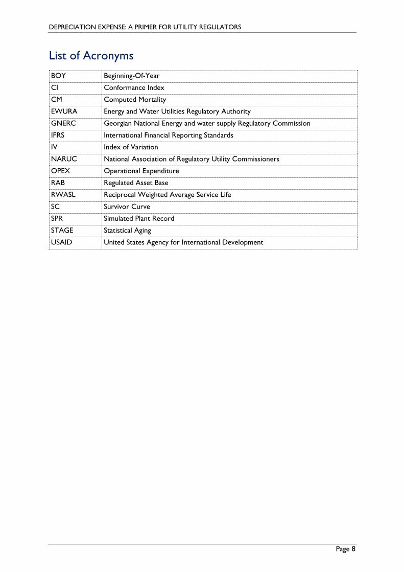
List of Acronyms
BOY Beginning-Of-Year
CI Conformance Index
CM Computed Mortality
EWURA Energy and Water Utilities Regulatory Authority
GNERC Georgian National Energy and water supply Regulatory Commission
IFRS International Financial Reporting Standards
IV Index of Variation
NARUC National Association of Regulatory Utility Commissioners
OPEX Operational Expenditure
RAB Regulated Asset Base
RWASL Reciprocal Weighted Average Service Life
SC Survivor Curve
SPR Simulated Plant Record
STAGE Statistical Aging
USAID United States Agency for International Development
DEPRECIATION EXPENSE: A PRIMER FOR UTILITY REGULATORS
Page 9
1. Introduction
With funding support from USAID, the NARUC is developing a Cost-Reflective Tariff Toolkit aimed at supporting policymakers, regulators, and utilities on the design and implementation of cost-reflective tariffs through effective engagement of the public and key stakeholders in the decision-making process. The Toolkit consists of several short primers providing practical information and guidance on specific elements and topics of cost-reflective tariffs to utility service regulators in emerging economies.
The development and application of cost-reflective tariffs, based on sound economic principles, is of crucial importance for safeguarding the financial viability of energy utilities and the electricity sector as a whole. It also ensures that appropriate incentives are in place for attracting necessary investments in the electricity sector.
1.1. Objective
The objective of this primer is to assist energy regulators working in emerging economies with building their understanding and knowledge of key concepts related to depreciation, and to support effective decision making when developing cost-reflective tariffs.
1.2. Scope
This primer presents key factors affecting allowed depreciation costs as well as alternative approaches and regulatory considerations when determining allowed depreciation in the context of cost-reflective tariffs for regulated entities operating in monopolistic market segments (e.g. network companies).
1.3. Organization
The primer is organized as follows:
Section 2 places depreciation in the context of tariff regulation.
Section 3 presents fundamental concepts and principles of regulatory depreciation.
Section 4 presents alternative cost allocation methods.
Section 5 presents the components of age-life methods.
Section 6 discusses alternative approaches for determining asset value.
Section 7 presents common techniques for calculating the service life of an asset.
Section 8 describes common methods for determining the depreciation rate.
Section 9 explains alternative asset grouping procedures.
Section 10 discusses overarching regulatory considerations concerning depreciation.
Section 11 concludes with final remarks.
Annex 1 presents numerical examples.
Annex II provides case studies of how regulators in Georgia and Tanzania determine allowed depreciation for electricity transmission systems as part of the utility’s tariff-setting process.
DEPRECIATION EXPENSE: A PRIMER FOR UTILITY REGULATORS
Page 10
2. Depreciation Overview
2.1. Tariff Regulation Context
The long-term objective of a regulated firm is to preserve its profitability and viability, as reflected in its financial statements. On the other hand, the long-term objective of the regulator is to deliver a safe, reliable, economic, sustainable, and environmentally responsible supply of energy to end-users, while at the same time ensuring the financial viability of the regulated utility.1 For this purpose, when setting tariffs and associated incentives, the regulator must consider their impact on end-users, while at the same time allowing the firm a reasonable opportunity to recover its operating costs and capital. The regulated firm must reconcile financial performance objectives with regulatory compliance.
2.2. Definition and Treatment of Depreciation
Depreciation is defined as the decrease in the value or worth of a fixed asset that occurs throughout its life, and is usually associated with utilizing the asset for the production of material goods or services. When determining depreciation of an asset over time, a systematic and rational approach should be adopted for the purpose of allocating the value of a depreciable asset over its life.
Depreciation, which refers to the periodic allocation of costs to reflect the use of tangible fixed assets such as buildings and equipment, is distinguished from amortization, which refers to the use of intangible assets such as patents, copyrights, leaseholds and goodwill. The focus of this primer is on depreciation, as regulators may or may not recognize intangible assets in the Regulated Asset Base (RAB) of regulated companies.2
In the context of statutory accounting, depreciation refers to the expense that a company is allowed to record in its financial accounts, according to legally binding rules, for the purpose of determining its taxable income. In the context of tariff regulation, which is the subject of this primer, depreciation refers to the expense that a regulated entity is allowed to recover through service tariffs. Regulatory depreciation shall correspond to an estimate of the annual cost that is incurred by ‘using up’ or ‘consuming’ the value of specific assets for the provision of the regulated service. Depreciation is one of the three main elements of a regulated entity’s Allowed Revenue, the annual revenue that the regulated utility is allowed to recover through its tariffs. Allowed Revenue is commonly determined as the sum of three individual ‘building blocks:’ the regulated entity’s operating costs (OPEX), depreciation (‘return of capital’), and a return on the invested capital (‘return on capital’).3 The government and regulatory authorities should work together with the aim to align
1 Specifically, regulatory decisions and rulemaking must balance the following requirements: serve demand growth and expand electricity access, ensure the financial viability of utilities, facilitate private investment, protect customer interests (particularly of vulnerable customers), support technical safety and maintain system reliability, enhance energy security and manage risk. 2 Amortization expenses associated with acquisition premia in particular may potentially not be included in the determination of a regulated entity’s Allowed Revenue, as they are linked to company-specific motivations and do not reflect any true economic costs of providing the regulated service. The recognition of amortization expenses associated with acquisition premia in a regulated entity’s Allowed Revenue would create an incentive for acquiring companies to raise their acquisition price, thus resulting in inflated tariffs and distorted price signals to customers. 3 Income tax should be included as a fourth building block element in the Allowed Revenue in case the allowed return (e.g. WACC) is in ‘post-tax’ terms. Otherwise, the regulated utility’s income tax obligation is accounted for by the ‘pre-tax’ allowed return so income tax should not be included as a separate building block element of Allowed Revenue.
DEPRECIATION EXPENSE: A PRIMER FOR UTILITY REGULATORS
Page 11
regulatory and statutory depreciation methodologies in order to ensure that consistent incentives are provided to the regulated companies.4 The allowed depreciation expense also facilitates the financing of investments required for the provision of the regulated service. Specifically, recovery of depreciation expenses through service tariffs ensures the financial viability of utilities by making available the necessary funds for repayment of capital borrowed through bank or bond financing. In the latter case, where such financing instruments are available, depositing depreciation expenses recovered over time in a ‘sinking fund’ enables the utility to pay off the bond upon its maturity (e.g. 30 years after the initial investment). Overall, in order to ensure that tariffs signal the true economic cost of providing the regulated service (see section 3 below), depreciation expenses should be used solely for allocating the cost associated with using an asset for the provision of the regulated service. This is highlighted in NARUC (1996, p.23):5
It is essential to remember that depreciation is intended only for the purpose of recording the periodic allocation of cost in a manner properly related to the useful life of the plant. It is not intended, for example, to achieve a desired financial objective or to fund modernization programs.
3. Fundamentals of Depreciation
3.1. Regulatory Depreciation Principles
Regulatory decisions and rulemaking concerning depreciation should adhere to the following key regulatory principles. • Economic efficiency: Tariffs should be designed so that regulated entities can expect to recover
the cost of efficiently incurred investments, while at the same time limiting the scope for unnecessarily high returns.6 A corollary of the latter is that, considering all different customer classes in aggregate, the regulated company should be allowed to recover the cost of its investments only once (i.e. customers should not have to pay for the same asset multiple times), in contrast to what may be observed in competitive markets. In other words, regulated entities shall be provided with appropriate incentives to invest in the assets that are necessary for delivering the regulated service at the desired level, while the true economic cost of providing the regulated service should be signaled via prices so as to ensure that customers make socially optimal decisions.
• Price stability and intergenerational equity: The profile of regulatory depreciation directly impacts the time profile of prices and thus the uncertainty that may be associated with price variations as well as the inter-temporal allocation of costs arising from the provision of the regulated service. The principles of price stability and intergenerational equity imply that the profile
4 For example, a regulatory approach aimed at incentivizing regulated companies to undertake investments through early recognition of depreciation expense in its Allowed Revenue (e.g. ‘Accelerated’ method resulting in higher charges in the first years of the service life of an asset, as discussed in section 8) might be diluted by a statutory approach of Straight-Line depreciation in case the additional depreciation proceeds allowed by the regulator are not deducted from taxable income. This would be the case if income tax is not included as a separate ‘building block’ item in the Allowed Revenue but instead is accounted for through the use of a pre-tax allowed return (e.g. pre-tax WACC). 5 NARUC. 1996. Public Utility Depreciation Practices. Washington, DC: National Association of Regulatory Utility
Commissioners. 6 Designing regulated tariffs is the process of allocating the cost of services provided between and within categories of customers (customer classes), reflecting the specific costs associated with the use of the system by each customer class.
DEPRECIATION EXPENSE: A PRIMER FOR UTILITY REGULATORS
Page 12
of regulatory depreciation chosen should aim to minimize price volatility and the associated risk, as well as ensure that costs are equitably allocated across time.
• Administrative simplicity: A simple approach to regulatory depreciation is preferred, for the
purpose of minimizing the administrative burden to the regulator as well as for ensuring that pricing decisions by the regulator can be easily followed and anticipated by energy sector stakeholders, including the regulated entity.
3.2. Basic Depreciation Concepts
There are two approaches for determining the value of depreciation: the ‘value’ concept and the ‘cost allocation’ concept. The value concept for determining regulatory depreciation is based on periodic estimations of the asset value. The decrease in the estimated value of the asset can be considered as a measure of the value of depreciation for the corresponding period. The estimation can be made either in terms of the replacement cost, the market value, or the earnings value of the asset, through physical inspections or sample checks regarding obsolescence, wear and tear, and inadequacy of the asset. However, the value concept is not commonly used for determining the value of regulatory depreciation as it is highly burdensome and creates significant uncertainty both for the regulator and the regulated utility. NARUC (1996, p.11-12) describes the significant drawbacks of the value concept approach:
It would (…) be a staggering undertaking to attempt such estimates on an annual basis for a complex and extensive utility plant. Therefore, the practice of conducting annual estimates has found little application in the utility industry. It is particularly cumbersome and inadequate because utilities need to record depreciation on a monthly basis for earnings and expense reports. A further complication, of course, is that major technological improvements tend to make questionable any year-to-year measure of depreciation that is determined by this process.
In the cost allocation concept, the original cost of an asset is treated as a prepaid expense. The value of regulatory depreciation is then determined by allocating this expense to specific accounting periods during the time the asset is providing service. The depreciation expense allocated in each accounting period is logged on the regulated entity’s income statement, while the unallocated amount, the ‘net asset value,’ is logged as an asset in the balance sheet. The cost allocation concept is considered the most appropriate, and it is the one that regulators use for determining the value of depreciation in the context of cost-reflective tariff setting. NARUC (1996, 12) highlights the advantages of the cost allocation concept approach:
The cost allocation concept satisfies the accounting principle of matching expense and revenues. On the income statement, the inflow of resources is revenue. The outflow is expense. Using up the productive capacity of assets in an accounting period is recorded in accounting records as depreciation expense.
The amount of money used to purchase the asset is the basis for the entry in accounting records. This amount is regarded as being definite and immediately determinable. The accounting objectives of verifiability and neutrality are also satisfied.
DEPRECIATION EXPENSE: A PRIMER FOR UTILITY REGULATORS
Page 13
4. Cost Allocation Methods
The main cost allocation methods are ‘age-life’ methods and ‘unit of production methods.’ Unit of production methods estimate depreciation costs on the basis of units of production (e.g. energy transmitted) rather than as a function of time. The underlying assumptions of unit of production methods are: • An asset’s capacity to provide the regulated service can be more accurately determined in
production units rather than in years of service life. • The depreciation expense associated with ‘using up’ or ‘consuming’ its value is more strongly
related to the asset’s level of utilization rather than its age. Age-life methods estimate depreciation costs as a function of time. Common to all age-life methods is an estimate of service life and an apportionment of expense by ‘using up’ or ‘consuming’ the value of specific assets to each year or accounting period so that the total cost is recovered over the life of the asset. Age-life methods will be the focus of this primer, as they are the most commonly used variant of the cost allocation concept, and the one that is most appropriate for the purpose of determining depreciation expenses of energy network infrastructure. NARUC (1996, p.52) draws attention to the advantages of age-life methods and the fact that this methodological approach is the one used almost universally for the determination of depreciation expenses:
Because reasonable estimates at any time are attainable, and age-life methods directly meet the depreciation objective, age-life methods are favored by all accounting, regulatory, and tax depreciation plans. Departures from age-life methods require specific justification, such as extraordinary obsolescence or consumption not related to age.
5. Age-Life Methods
Age-life methods require estimates of the following elements (each discussed in further detail in sections 6, 7, and 8): • A measure of the asset’s initial value and net salvage value (i.e. of the proceeds received from
the disposition of the retired asset upon completion of its service life, less the costs of removal), discussed in section 6.
• A measure of the asset’s service life (i.e. of the period during which the asset will be able to provide the regulated service with minimal or no requirement for replacement or maintenance investments), such as average service life or remaining life, discussed in section 7.
• A decision on the type of annual rate based on which the total cost of the asset will be recovered during its service life, discussed in section 8.
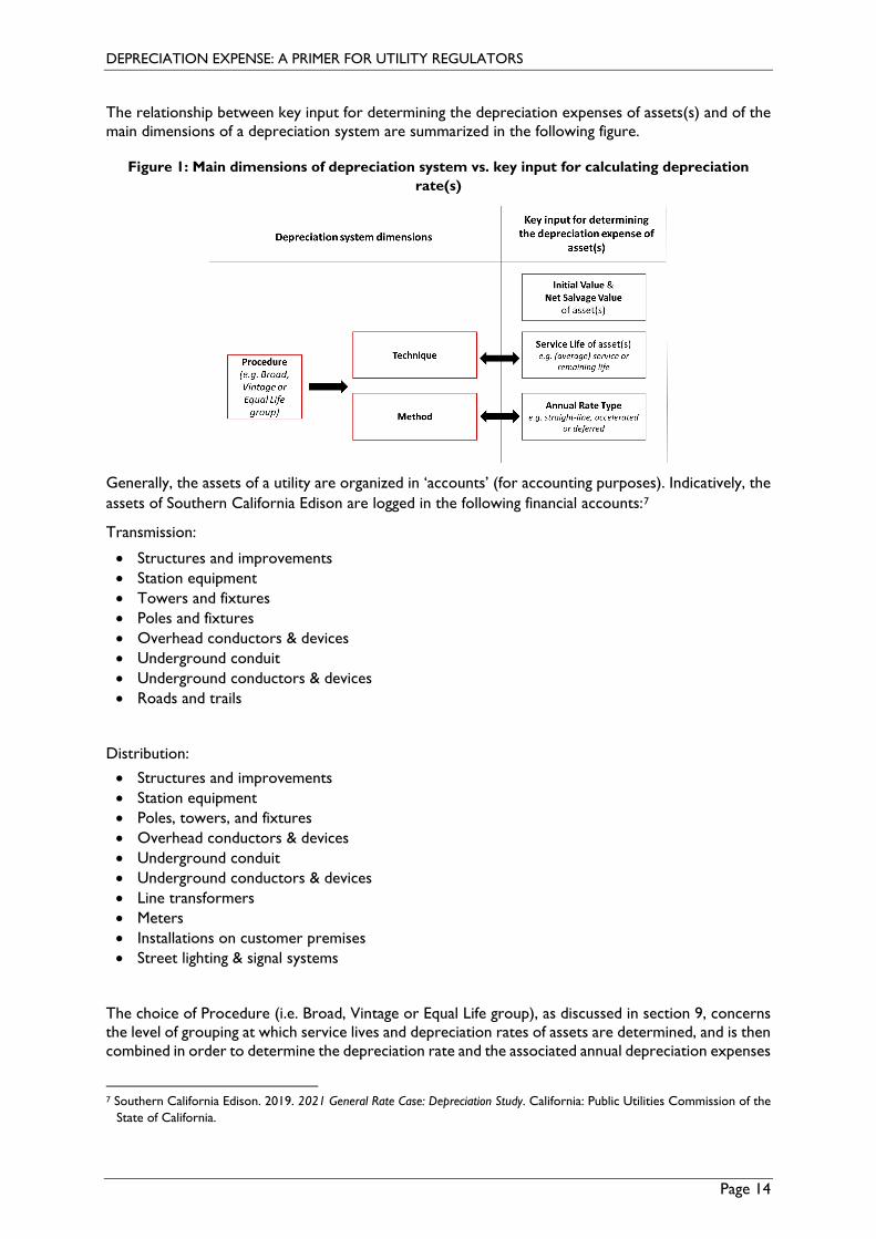
The three basic dimensions commonly used to define a utility’s depreciation system (i.e. the systematic approach for allocating the value of depreciable assets over their life) are:
1. Method: concerns the choice of the annual rate type (i.e. Straight-Line, Accelerated or Deferred methods)
2. Procedure: concerns the choice for grouping of individual asset units under a depreciation class (e.g. Broad, Vintage or Equal Life group) and is discussed in section 9
3. Technique: concerns the choice for the asset life measure (e.g. average life or remaining life)
DEPRECIATION EXPENSE: A PRIMER FOR UTILITY REGULATORS
Page 14
The relationship between key input for determining the depreciation expenses of assets(s) and of the main dimensions of a depreciation system are summarized in the following figure.
Figure 1: Main dimensions of depreciation system vs. key input for calculating depreciation rate(s)
Generally, the assets of a utility are organized in ‘accounts’ (for accounting purposes). Indicatively, the assets of Southern California Edison are logged in the following financial accounts:7
Transmission:
• Structures and improvements • Station equipment • Towers and fixtures • Poles and fixtures • Overhead conductors & devices • Underground conduit • Underground conductors & devices • Roads and trails
Distribution:
• Structures and improvements • Station equipment • Poles, towers, and fixtures • Overhead conductors & devices • Underground conduit • Underground conductors & devices • Line transformers • Meters • Installations on customer premises • Street lighting & signal systems
The choice of Procedure (i.e. Broad, Vintage or Equal Life group), as discussed in section 9, concerns the level of grouping at which service lives and depreciation rates of assets are determined, and is then combined in order to determine the depreciation rate and the associated annual depreciation expenses
7 Southern California Edison. 2019. 2021 General Rate Case: Depreciation Study. California: Public Utilities Commission of the
State of California.
DEPRECIATION EXPENSE: A PRIMER FOR UTILITY REGULATORS
Page 15
for each account. In other words, a different rate of depreciation is first estimated for each group. These depreciation rates are then weighted (taking into account the size of each group), to determine the average depreciation rate of the account (e.g. ‘poles, towers, and fixtures’) to which the groups belong.
6. Asset Value
The initial value of an asset is a key element of age-life methods for determining regulatory depreciation. Additionally, an asset may need to be reevaluated during its life in order to more accurately reflect the true economic value of ‘using up’ or ‘consuming’ this asset to provide the regulated service. The estimation of asset value can be based on three approaches:8
1. Historic costs (i.e. original asset costs) 2. Replacement costs (i.e. current asset costs) 3. Market value of the asset
• Historic costs: the original cost of acquiring an asset. This approach is more relevant for new assets (i.e. newly built infrastructure and equipment). When determining the depreciable value of pre-existing assets, following a change in the ownership or legal status of the regulated company (e.g. unbundling), the depreciation reserve accumulated to date must be subtracted from the original cost of purchasing the asset or it should be appropriately reflected in the acquiring company’s financial accounts.
As discussed in ERRA (2009), this approach has the following advantages: it is efficient, objective, and can be easily audited as it is based on the accounting costs recorded in the company’s financial statements rather than on expert assessments.9 On the other hand, data on the original cost of acquiring old assets may not be available (e.g. when the value of assets of a newly formed network company needs to be determined following its unbundling from a vertically integrated utility). Additionally, this approach does not always provide an accurate estimate of the asset’s true economic value, leading to underestimation when there is high inflation and overestimation when there is rapid technological change. Finally, this approach may lead to lumpy and/ or unstable tariffs, since the allowed depreciation, which is re-calculated following the purchase of new assets (valued in current market prices), may be significantly higher than the previously allowed depreciation (based on previously acquired assets valued at historic cost). A specific variant of the historic cost approach is often applied in inflationary environments, in which the value of assets is periodically re-adjusted in line with an inflation index, either annually or at specific intervals.10
8 For the vast majority of regulators, the asset valuation approach used for determining the allowed depreciation is identical to the approach used for estimating the value of the RAB, which is in turn used for determining the entity’s allowed return on invested capital. 9 ERRA. 2009. Determination of the Regulatory Asset Base after Revaluation of License Holder’s Assets. Chart of Account. Budapest:
Energy Regulators Regional Association. 10 This variant of the historic cost approach is distinct from regulatory approaches where RAB is inflation-indexed due to the use of a ‘real’ return on capital (i.e. excluding inflation). In the variant referred to in the context of this Primer, the regulator chooses to compensate the regulated company for the decline in the real value of its assets, over and above the nominal return on its capital (i.e. which already accounts for inflation in the regulated entity’s allowed return of equity and debt).
DEPRECIATION EXPENSE: A PRIMER FOR UTILITY REGULATORS
Page 16
Concerning entities whose functional currency is the currency of a hyperinflationary economy, defined as one with cumulative inflation over three years of 100% or more, International Accounting Standard 29 (IAS 29) of the International Financial Reporting Standards (IFRS) applies. IAS 29 specifies that:
Financial statements (…) must be expressed in units of the functional currency current as at the end of the reporting period. Restatement to current units of currency is made using the change in a general price index. An entity must disclose the fact that the financial statements have been restated, the price index used for restatement, and whether the financial statements are prepared on the basis of historical costs or current costs.11
When determining regulatory depreciation in hyperinflationary environments, application of IAS 29 overcomes the underestimation of an asset’s economic value and thus of allowed depreciation, which would arise if the unadjusted historic cost of the asset were to be used. On the other hand, conditions of hyperinflation aggravate the conflict between the objectives of the regulator to a) keep the tariffs stable over time and b) to secure recovery of the investment. In most cases, equipment and machinery are purchased in international currency, and any adjustments in the Allowed Revenue as a result of hyperinflation may require a significant increase in the value to be recovered and lead to a rise in tariffs. Therefore, the application of the IFRS should be accompanied with other regulatory measures (e.g. prolonging the depreciation period) to mitigate the negative impact of hyperinflation on the level of tariffs.
• Replacement costs: the cost of replacing an existing asset with equivalent infrastructure or equipment, having the same capability and capacity to provide the regulated service, minus the associated accumulated depreciation reflecting the life of the existing asset.
This approach is more relevant for pre-existing assets, the value of which needs to be re-determined due to a change in the ownership or legal status of the regulated company that may also change the associated regulatory framework. For example, an existing network company may be privatized, or it may be established following unbundling from a vertically integrated utility. The latter case may also be linked with the development of an open access framework and use-of-system tariffs for the respective network. A reevaluation of the regulated network company’s assets is often warranted in such cases in order to ensure that the true economic cost of providing the service is reflected in tariffs and in their expected revenue and profits. The advantages and disadvantages of this approach are discussed in ERRA (2009). Τhis approach leads to a more accurate estimate of the asset’s true economic value, as compared to the historic cost approach, and thus to more efficient decisions by customers (e.g. in terms of consumption) as well as by the regulated company (e.g. in terms of long-term investments). It also leads to smoother variation in Allowed Revenue and tariffs following the purchase of new assets. On the other hand, this approach may be more costly and subjective as it is based on assessments carried out by expert evaluators and requires collection of detailed data and information.
• Market value: based on the present value of future expected net cash flows resulting from the provision of regulated services that are associated with the operation of an asset.
11 “IAS 29 Financial Reporting in Hyperinflationary Economies.” IFRS. https://www.ifrs.org/issued-standards/list-of-standards/ias-29-financial-reporting-in-hyperinflationary-economies/
DEPRECIATION EXPENSE: A PRIMER FOR UTILITY REGULATORS
Page 17
This estimate leads to a more accurate estimate of the asset’s true economic value, as compared to the historic cost approach. However, the major disadvantage of this approach is that it is circular since the allowed depreciation is an input to the future expected net cash flows used for determining the asset’s market value (and in turn the level of allowed depreciation).
Aside from considerations related to inflation, and under normal circumstances (i.e. not involving a change in the regulated entity’s legal or ownership status or a major change in the regulatory framework), the options available to the regulator for the purpose of determining the allowed depreciation (as well as the return on capital) are:
• Require the regulated entity to re-evaluate its assets at regular intervals based on replacement costs, according to specific rules established by the regulator.
• Do not allow any revaluation of assets.
The main advantage of the replacement cost approach is that the resulting tariff better reflects the ‘true’ cost of providing the regulated service, thus leading to a more efficient allocation of resources, primarily in terms of customer choices concerning their level of consumption, as well as in terms of investment decisions by the regulated entity. The main disadvantage of this approach is that it may create uncertainty for the regulated entity concerning the recovery of its capital (as well as the achievement of its required return on capital). This will be reflected adversely on customer tariffs, as a higher return on capital will be required by the regulated entity in order to compensate for this risk.12 In practice, regulators often use a hybrid approach combining the use of historic costs for new assets, with ad-hoc or periodic re-valuations using replacement costs. On the other hand, it is preferable that the regulator use a consistent approach. Consistency provides certainty to the regulated entity that it will recover its capital through allowed depreciation (as well as its return on capital), thus minimizing the level of risk associated with its investment and avoiding tariff increases. Salvage value In order to calculate the asset value to be used for determining the allowed depreciation expense, the net salvage value of the asset at its retirement should be deducted from the initial asset value (or any subsequent re-valuation). The net salvage value of an asset is the amount that can be received for a retired asset if it is sold or reused for another purpose within the utility (gross salvage value), over and above any associated removal cost. Sources of gross salvage value include the sale of parts and material of the retired asset as scrap, or sale of the asset for reuse. For example, retired copper conductors may be sold as raw material. Equipment may be sold to other companies who can refurbish them for resale or their own use. Alternatively, when an asset is retired from providing the regulated service, it can be used by the utility for other purposes. In any case, the value of the salvage, at the time of retirement from providing the regulated service, needs to be determined based on the asset’s replacement cost or market value. If the asset is put to other uses by the utility, a measure of the asset’s life that is associated with the alternative use should also be determined, and the corresponding depreciation schedule be calculated again. The cost of removal refers to the cost of demolishing, dismantling or removing an asset and consists primarily of labor and other costs associated with transportation and handling as well as costs arising
12 This is especially the case if the re-evaluation also includes an optimization assessment of the regulated entity’s assets which can potentially result in a regulatory decision to exclude a particular asset from the Allowed Revenue calculation if it is deemed that the asset in question is no longer necessary for providing the regulated service.
DEPRECIATION EXPENSE: A PRIMER FOR UTILITY REGULATORS
Page 18
due to the need for waste disposal or environmental remediation. The cost of removal also needs to be estimated in order to determine the asset’s net salvage value that will enter the calculation of the depreciation rate. In practice, the value of scrap for the majority of transmission or distribution assets is likely to be only limited or nil. In contrast, removal costs are often significant, thus resulting in a negative net salvage value. Therefore, the resulting cost to be depreciated often exceeds the initial asset value.13
7. Asset Life
7.1. Asset Life Concepts
The asset’s life is another key element of age-life methods for determining regulatory depreciation. In the context of tariff regulation, an asset’s life is effectively determined by the time the asset is retired from providing the regulated service. The time an asset is retired from providing the regulated service, or reaches the end of its life, may depend on ‘physical’ or ‘functional’ factors. Physical factors leading to the retirement of an asset include:
• Wear and tear: the damage that naturally and inevitably occurs as a result of normal wear or aging of an asset.
• Decay or deterioration: the gradual damage caused by environmental factors such as moisture, temperature, solar radiation, air movement and pressure, precipitation, and intrusion by insects.
• Extreme climate events and accidents: the damage due to exceptional natural phenomena (e.g. storm, flooding, hurricane, etc.) or due to accidents caused by human, animals, or vegetation.
Functional factors leading to the retirement of an asset relate to market, regulatory, policy and technological developments which make the operation of the asset unprofitable or inefficient, including: • Inadequacy: The asset lacks the capacity to provide the regulated service due to changes in market
preferences or demand. In such case, it might be preferable to replace the entire asset rather than make additions. For example, replacement rather than extension of a substation may be required if the existing substation is insufficient to accommodate new equipment such as switchgear, and to ensure that supply is not interrupted by keeping the existing substations operational while the new is installed.
• Obsolescence: The asset becomes uneconomical, inefficient, or otherwise unfit to provide the regulated service due to technological developments. For example, replacement of conventional meters by smart metering devices may be required in order to improve identification and monitoring of supply interruptions and the associated corrective actions.
• Public authorities: The asset needs to be replaced due to a request by public authorities (e.g. due to interference with public uses or works) or due to changing policies and regulations (e.g. change in service, environmental or safety standards).
Based on the distinction between ‘physical’ or ‘functional’ factors leading to the retirement of an asset, two asset life concepts are defined:
13 This is especially the case when historic costs are used for determining the initial value of assets and no adjustment factor is applied to this value to account for inflation. In such cases, since salvage value is estimated on the basis of current prices, while initial asset value is determined on the basis of prices at the time of installation, it is often the case that the former is a significant part of the total cost to be depreciated over an asset’s life.
DEPRECIATION EXPENSE: A PRIMER FOR UTILITY REGULATORS
Page 19
1. ‘Physical Life:’ period over which an asset remains functional (i.e. until it physically deteriorates to the point of being no longer functional irrespective of whether it is inadequate or technologically obsolete).
2. ‘Service Life:’ period over which an asset can be used for providing the regulated service (i.e. until it becomes inadequate or technologically obsolete or needs to be replaced due to changing policies and regulations).
In reality, functional factors tend to be the most frequent causes leading to the retirement of assets, thus an asset’s service life tends to be the most appropriate and common approach to the determination of an asset’s life. Concerning the treatment of service life for determining the allowed depreciation expenses of a regulated entity, there are two main approaches: the ‘Whole Life’ technique and the ‘Remaining Life’ technique. Whole Life technique
The Whole Life technique uses the total service life of an asset to calculate the depreciation expense (i.e. the allocation of an asset’s value) over its whole life. The annual depreciation expense is calculated for the whole life of the asset and applied going forward. Indicatively, when using the Whole Life technique and applying a ‘Straight-Line’ method for determining depreciation (discussed in detail in section 8) the salvage and removal costs need to be subtracted from the initial value of the asset, and divided by the asset’s service life:
𝐴𝐴𝐴𝐴𝐴𝐴𝐴𝐴𝐴𝐴𝐴𝐴 𝐷𝐷𝐷𝐷𝐷𝐷𝐷𝐷𝐷𝐷𝐷𝐷𝐷𝐷𝐴𝐴𝐷𝐷𝐷𝐷𝐷𝐷𝐴𝐴 =𝐼𝐼𝐴𝐴𝐷𝐷𝐷𝐷𝐷𝐷𝐴𝐴𝐴𝐴 𝑉𝑉𝐴𝐴𝐴𝐴𝐴𝐴𝐷𝐷 𝐷𝐷𝑜𝑜 𝐴𝐴𝐴𝐴𝐴𝐴𝐷𝐷𝐷𝐷 − (𝑆𝑆𝐴𝐴𝐴𝐴𝑆𝑆𝐴𝐴𝑆𝑆𝐷𝐷 − 𝑅𝑅𝐷𝐷𝑅𝑅𝐷𝐷𝑆𝑆𝐴𝐴𝐴𝐴 𝐶𝐶𝐷𝐷𝐴𝐴𝐷𝐷)
𝑇𝑇𝐷𝐷𝐷𝐷𝐴𝐴𝐴𝐴 𝑆𝑆𝐷𝐷𝐷𝐷𝑆𝑆𝐷𝐷𝐷𝐷𝐷𝐷 𝐿𝐿𝐷𝐷𝑜𝑜𝐷𝐷 (1)
The resulting depreciation value is applied annually, throughout the asset’s life. However, it is likely that the service life assigned to the asset turns out to be incorrect (see discussion on estimation of service life in section 9.2) or that the salvage value and removal costs are not accurate.
The major disadvantage of the Whole Life technique is that it will result in a ‘depreciation reserve imbalance’ (i.e. the accumulated depreciation might be higher or lower than it should). To correct such over-accrual or under-accrual of depreciation a special depreciation factor14 (positive or negative) may be allowed to be added to the estimated one.
Remaining Life technique
The Remaining Life technique uses the remaining service life of the asset over which the undepreciated initial value of the asset less the salvage and removal costs, is allocated. Indicatively, when using the Remaining Life technique and applying a Straight-Line method for determining depreciation (discussed in detail in section 8), accumulated depreciation to date (i.e. the depreciation reserve) as well as the salvage and removal costs need to be subtracted from the initial value of the asset, and divided by the asset’s remaining life:
𝐴𝐴𝐴𝐴𝐴𝐴𝐴𝐴𝐴𝐴𝐴𝐴 𝐷𝐷𝐷𝐷𝐷𝐷𝐷𝐷𝐷𝐷𝐷𝐷𝐷𝐷𝐴𝐴𝐷𝐷𝐷𝐷𝐷𝐷𝐴𝐴 = 𝐼𝐼𝐴𝐴𝐷𝐷𝐷𝐷𝐷𝐷𝐴𝐴𝐴𝐴 𝑉𝑉𝐴𝐴𝐴𝐴𝐴𝐴𝐷𝐷 𝐷𝐷𝑜𝑜 𝐴𝐴𝐴𝐴𝐴𝐴𝐷𝐷𝐷𝐷 − (𝑆𝑆𝐴𝐴𝐴𝐴𝑆𝑆𝐴𝐴𝑆𝑆𝐷𝐷 − 𝑅𝑅𝐷𝐷𝑅𝑅𝐷𝐷𝑆𝑆𝐴𝐴𝐴𝐴 𝐶𝐶𝐷𝐷𝐴𝐴𝐷𝐷) − 𝑅𝑅𝐷𝐷𝐴𝐴𝐷𝐷𝐷𝐷𝑆𝑆𝐷𝐷
𝑅𝑅𝐷𝐷𝑅𝑅𝐴𝐴𝐷𝐷𝐴𝐴𝐷𝐷𝐴𝐴𝑆𝑆 𝑆𝑆𝐷𝐷𝐷𝐷𝑆𝑆𝐷𝐷𝐷𝐷𝐷𝐷 𝐿𝐿𝐷𝐷𝑜𝑜𝐷𝐷 (2)
The advantage of the Remaining Life technique is that any necessary adjustments to the annual depreciation because of required corrections to the estimated service life or to the salvage value and removal costs, are accrued automatically over the remaining life of the asset.
As discussed in section 9, depreciation expenses tend to be estimated for groups of assets with similar characteristics in aggregate, rather than for each asset unit individually, as detailed data for each unit
14 Commonly referred to as ‘amortization’ factor.
DEPRECIATION EXPENSE: A PRIMER FOR UTILITY REGULATORS
Page 20
is often impractical and highly expensive to maintain. When referring to groups of assets rather than individual assets, the above formulas for the Whole Life and Remaining Life technique are replaced by equivalent aggregate values for the assets in the group, while service life measures are replaced by average figures for the whole group, specifically ‘average service life’ and ‘average remaining service life.’
7.2. Estimating Service Life
The values of service life used for the various assets of the regulated entity, in order to determine the allowed depreciation expense, can range from assumptions by the company management (following guidance from the regulator) or directly by the regulator, to informed assessments based on complex technical mathematical models. The approach used for estimating the average or the remaining service life of an asset or a group of assets with similar life and mortality characteristics, depends on the availability of statistical historical data on the age of each asset item (i.e. ‘aged’ data) by the regulated entity. Aged data require a detailed record of the age of each asset item, from the date of installation to the date of retirement. However, for some asset types that involve numerous items it may be too expensive or impractical to record the exact age of each unit. In such cases, data are ‘unaged’ and contain only annual monetary amounts of installations and retirements. Actuarial methods applied to aged data
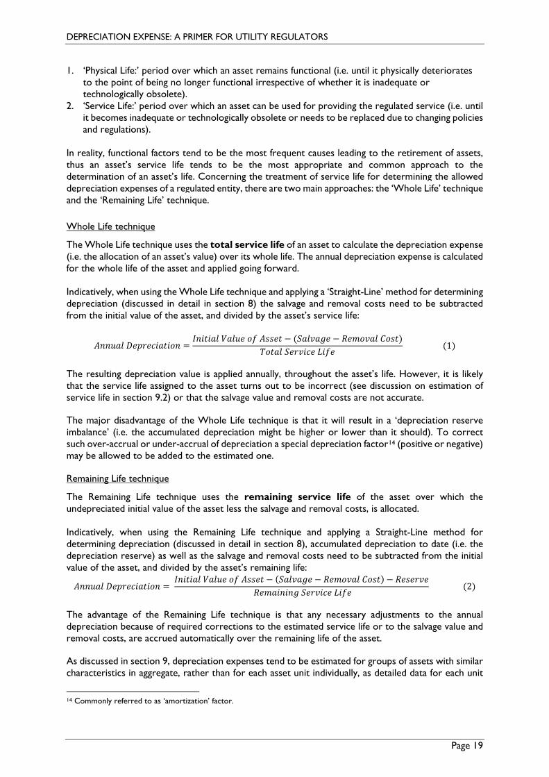
Life Analysis When a complete set of aged data is available, it is straightforward to analyze the ‘mortality’ characteristics of assets (i.e. the age at which assets within a certain group retire) using ‘actuarial’ methods. Actuarial methods are based on historic statistical data and produce associated ‘survivor curves’ required for estimating the average life and the average remaining life of a group of assets. Survivor curves depict the % of assets (in number or monetary units) within a group that are reaching a particular age. An example of a survivor curve is shown in the following figure. From this figure it can be inferred that approximately 40% of the assets in the group will survive to reach 20.5 years of age, or in other words they will not be retired before they reach 20.5 years of age.
Figure 2: Example of survivor curve
The same information can be depicted using a ‘retirement frequency curve’ showing the probability that an asset will retire at a particular age.
DEPRECIATION EXPENSE: A PRIMER FOR UTILITY REGULATORS
Page 21
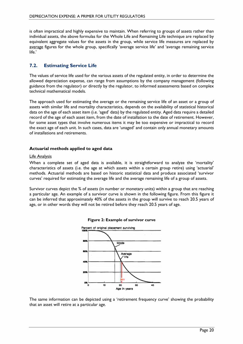
Figure 3: Example of survivor frequency curve
The key value of survivor curves (SC) is that they enable the calculation of the group’s average service life using the following formula, which effectively represents the average age of retirement weighted by the % of assets retired at each age:
𝐴𝐴𝑆𝑆𝐷𝐷𝐷𝐷𝐴𝐴𝑆𝑆𝐷𝐷 𝑆𝑆𝐷𝐷𝐷𝐷𝑆𝑆𝐷𝐷𝐷𝐷𝐷𝐷 𝐿𝐿𝐷𝐷𝑜𝑜𝐷𝐷 =𝐴𝐴𝐷𝐷𝐷𝐷𝐴𝐴 𝐴𝐴𝐴𝐴𝑢𝑢𝐷𝐷𝐷𝐷 𝑆𝑆𝐶𝐶 𝑜𝑜𝐷𝐷𝐷𝐷𝑅𝑅 𝐴𝐴𝑆𝑆𝐷𝐷 0 𝐷𝐷𝐷𝐷 𝑅𝑅𝐴𝐴𝑚𝑚
100% (3)
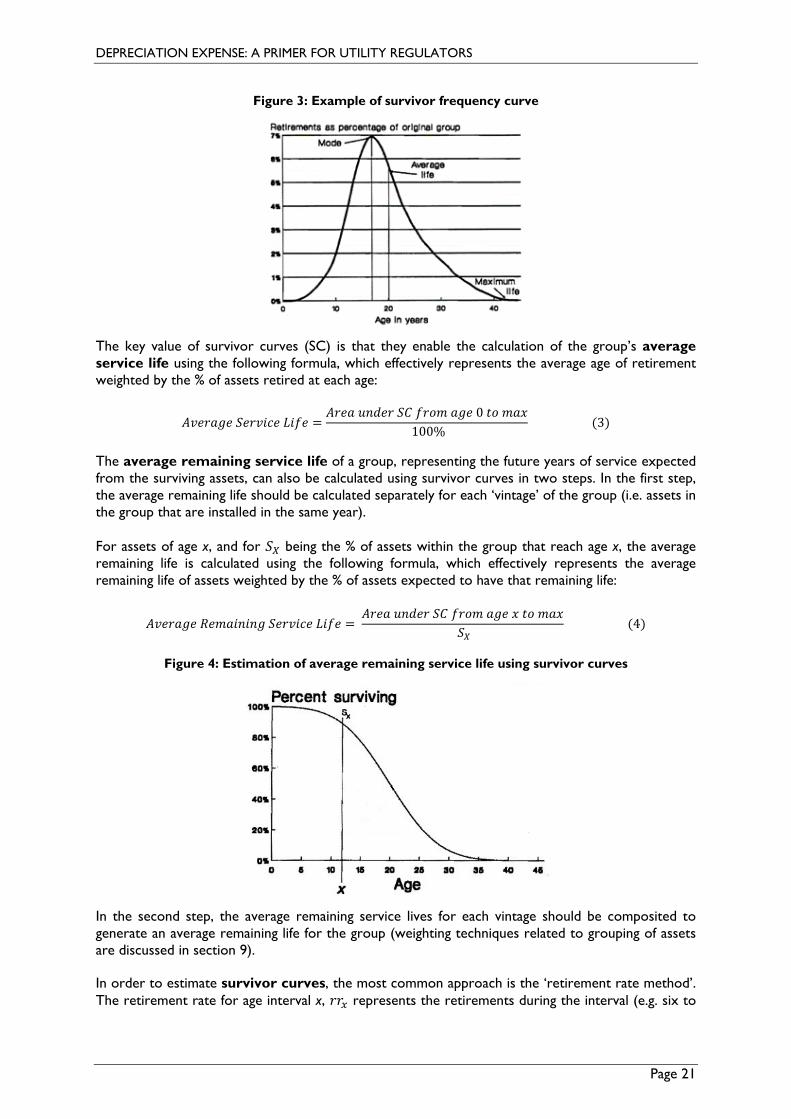
The average remaining service life of a group, representing the future years of service expected from the surviving assets, can also be calculated using survivor curves in two steps. In the first step, the average remaining life should be calculated separately for each ‘vintage’ of the group (i.e. assets in the group that are installed in the same year). For assets of age x, and for 𝑆𝑆𝑋𝑋 being the % of assets within the group that reach age x, the average remaining life is calculated using the following formula, which effectively represents the average remaining life of assets weighted by the % of assets expected to have that remaining life:
𝐴𝐴𝑆𝑆𝐷𝐷𝐷𝐷𝐴𝐴𝑆𝑆𝐷𝐷 𝑅𝑅𝐷𝐷𝑅𝑅𝐴𝐴𝐷𝐷𝐴𝐴𝐷𝐷𝐴𝐴𝑆𝑆 𝑆𝑆𝐷𝐷𝐷𝐷𝑆𝑆𝐷𝐷𝐷𝐷𝐷𝐷 𝐿𝐿𝐷𝐷𝑜𝑜𝐷𝐷 = 𝐴𝐴𝐷𝐷𝐷𝐷𝐴𝐴 𝐴𝐴𝐴𝐴𝑢𝑢𝐷𝐷𝐷𝐷 𝑆𝑆𝐶𝐶 𝑜𝑜𝐷𝐷𝐷𝐷𝑅𝑅 𝐴𝐴𝑆𝑆𝐷𝐷 𝑚𝑚 𝐷𝐷𝐷𝐷 𝑅𝑅𝐴𝐴𝑚𝑚
𝑆𝑆𝑋𝑋 (4)
Figure 4: Estimation of average remaining service life using survivor curves
In the second step, the average remaining service lives for each vintage should be composited to generate an average remaining life for the group (weighting techniques related to grouping of assets are discussed in section 9).
In order to estimate survivor curves, the most common approach is the ‘retirement rate method’. The retirement rate for age interval x, 𝐷𝐷𝐷𝐷𝑥𝑥 represents the retirements during the interval (e.g. six to
DEPRECIATION EXPENSE: A PRIMER FOR UTILITY REGULATORS
Page 22
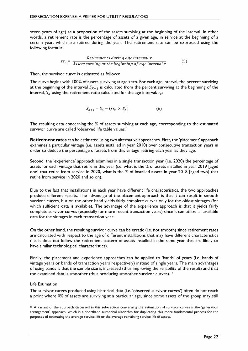
seven years of age) as a proportion of the assets surviving at the beginning of the interval. In other words, a retirement rate is the percentage of assets of a given age, in service at the beginning of a certain year, which are retired during the year. The retirement rate can be expressed using the following formula:
𝐷𝐷𝐷𝐷𝑥𝑥 = 𝑅𝑅𝐷𝐷𝐷𝐷𝐷𝐷𝐷𝐷𝐷𝐷𝑅𝑅𝐷𝐷𝐴𝐴𝐷𝐷𝐴𝐴 𝑢𝑢𝐴𝐴𝐷𝐷𝐷𝐷𝐴𝐴𝑆𝑆 𝐴𝐴𝑆𝑆𝐷𝐷 𝐷𝐷𝐴𝐴𝐷𝐷𝐷𝐷𝐷𝐷𝑆𝑆𝐴𝐴𝐴𝐴 𝑚𝑚
𝐴𝐴𝐴𝐴𝐴𝐴𝐷𝐷𝐷𝐷𝐴𝐴 𝐴𝐴𝐴𝐴𝐷𝐷𝑆𝑆𝐷𝐷𝐴𝐴𝑆𝑆 𝐴𝐴𝐷𝐷 𝐷𝐷ℎ𝐷𝐷 𝑏𝑏𝐷𝐷𝑆𝑆𝐷𝐷𝐴𝐴𝐴𝐴𝐷𝐷𝐴𝐴𝑆𝑆 𝐷𝐷𝑜𝑜 𝐴𝐴𝑆𝑆𝐷𝐷 𝐷𝐷𝐴𝐴𝐷𝐷𝐷𝐷𝐷𝐷𝑆𝑆𝐴𝐴𝐴𝐴 𝑚𝑚 (5)
Then, the survivor curve is estimated as follows:
The curve begins with 100% of assets surviving at age zero. For each age interval, the percent surviving at the beginning of the interval 𝑆𝑆𝑋𝑋+1 is calculated from the percent surviving at the beginning of the interval, 𝑆𝑆𝑋𝑋 using the retirement ratio calculated for the age interval𝐷𝐷𝐷𝐷𝑥𝑥 :
𝑆𝑆𝑋𝑋+1 = 𝑆𝑆𝑋𝑋 − (𝐷𝐷𝐷𝐷𝑥𝑥 × 𝑆𝑆𝑋𝑋) (6)
The resulting data concerning the % of assets surviving at each age, corresponding to the estimated survivor curve are called ‘observed life table values.’ Retirement rates can be estimated using two alternative approaches. First, the ‘placement’ approach examines a particular vintage (i.e. assets installed in year 2010) over consecutive transaction years in order to deduce the percentage of assets from this vintage retiring each year as they age. Second, the ‘experience’ approach examines in a single transaction year (i.e. 2020) the percentage of assets for each vintage that retire in this year (i.e. what is the % of assets installed in year 2019 [aged one] that retire from service in 2020, what is the % of installed assets in year 2018 [aged two] that retire from service in 2020 and so on). Due to the fact that installations in each year have different life characteristics, the two approaches produce different results. The advantage of the placement approach is that it can result in smooth survivor curves, but on the other hand yields fairly complete curves only for the oldest vintages (for which sufficient data is available). The advantage of the experience approach is that it yields fairly complete survivor curves (especially for more recent transaction years) since it can utilize all available data for the vintages in each transaction year. On the other hand, the resulting survivor curve can be erratic (i.e. not smooth) since retirement rates are calculated with respect to the age of different installations that may have different characteristics (i.e. it does not follow the retirement pattern of assets installed in the same year that are likely to have similar technological characteristics). Finally, the placement and experience approaches can be applied to ‘bands’ of years (i.e. bands of vintage years or bands of transaction years respectively) instead of single years. The main advantages of using bands is that the sample size is increased (thus improving the reliability of the result) and that the examined data is smoother (thus producing smoother survivor curves).15
Life Estimation The survivor curves produced using historical data (i.e. ‘observed survivor curves’) often do not reach a point where 0% of assets are surviving at a particular age, since some assets of the group may still 15 A variant of the approach discussed in this sub-section concerning the estimation of survivor curves is the ‘generation arrangement’ approach, which is a shorthand numerical algorithm for duplicating this more fundamental process for the purposes of estimating the average service life or the average remaining service life of assets.
DEPRECIATION EXPENSE: A PRIMER FOR UTILITY REGULATORS
Page 23
be in service beyond the maximum age at which assets have historically retired. In other words, particular vintages may reach ages between 55 and 60 years and still be in service, while the maximum recorded age of retirement in the group may be 54. In this case, the observed survivor curve is termed a ‘stub.’ This is important, as the complete curve is required in order to estimate the average service life (or average remaining service life) of a group, which is represented by the area under the curve. In this case, the observed survivor curve must be smoothed and extended to 0% surviving. As noted in NARUC (1996, p. 120):
The longer the stub, the more reliable the resulting curve fit and extension. As a result, the analyst may be forced to choose between a more reliable longer stub, which by necessity reflects older data, and a less reliable shorter stub, which reflects more recent vintages and, therefore, is more likely to reflect the future. It is generally considered desirable to have the stub curve drop below 50% surviving.
The methods generally used to smooth irregularities in the observed data or to extend a curve where data are lacking can be categorized as follows:
• Smoothing and extending the observed data (e.g. observed life table data, frequency curve, or
retirement ratios) using the Gompertz - Makeham formula.
• Mathematically matching generalized survivor curves (i.e. curve shapes) to the observed life table values: o The most widely used standard curve sets are the ‘Iowa’ curves originally conceived by Edwin
Kurtz and developed by Robley Winfrey (1931 and 1935).16 General classes of curves include L, S, R, and O and several sub-types, leading to approximately 32 standard curves.
o ‘Bell’ curves developed by the Bell telephone companies (NARUC, 1996). o ‘H’ curves by Bradford Kimball (1947) of the New York Public Service Commission.17
• Visually matching generalized survivor curves to the observed life table values, based on the analyst’s judgement. This approach is more time-consuming and less precise than mathematical matching, and is used less often.
Semi-actuarial methods applied to un-aged data
When the utility’s asset records and accounts do not contain the age of assets upon retirement, other methods termed ‘semi-actuarial’ are used to estimate the average service life and the average remaining service life of assets. The methods used can be categorized as follows: • The ‘Simulated Plant Record’ (SPR) (Bauhan, 1948) is the most commonly used method when only
un-aged data is available.18 The method indicates the generalized survivor curves that best represent the life characteristics of assets in each group. The selection of curves is based upon the closeness of the match between actual and simulated annual amounts and is measured by the Conformance Index (CI) or the Index of Variation (IV).
16 Winfrey, Robley, and Edwin B. Kurtz. 1931. “Life Characteristics of Physical Property.” “Bulletin 103,” Iowa Engineering
Experiment Station.
Winfrey, Robley. 1935 (Revised in 1967). “Statistical Analyses of Industrial Property Retirements.” Originally printed as “Bulletin 125.” Ames, Iowa: Engineering Research Institute, Iowa State University.
17 Kimball, Bradford F. 1947. “A System of Life Tables for Physical Property Based on the Truncated Normal Distribution.” Econometrica 15, no. 4: 342-360.
18 Bauhan, Alex. 1948. “Simulated Plant-Record Method of Life Analysis of Utility Plant for Depreciation-Accounting Purposes.” Land Economics 24, no. 2 (May): 129-136.
DEPRECIATION EXPENSE: A PRIMER FOR UTILITY REGULATORS
Page 24
These measures are based upon the ‘least squares’ method, which is a standard approach in regression analysis to find the best fit for a set of data points. The least square method aims to identify the fit (i.e. the curve) that minimizes the sum of the squares of the difference between actual and estimated data points. The most common type of generalized curves used in SPR methods are Iowa curves. The SPR method uses one of three different models to indicate a survivor curve:
o ‘Balance’ model: the generalized curves are ranked according to their ability to simulate actual annual asset balances for specified test years.
o ‘Period retirements’ model: the generalized curves are ranked according to their ability to simulate asset retirement for a specified period.
o ‘Annual retirements’ model: the generalized curves are ranked according to their ability to simulate annual asset retirements for specified test years.
• ‘Statistical Aging’ (STAGE) (ICC, 1985)19 and ‘Computed Mortality’ (CM) (Carver, 1989)20 models are used to simulate missing aged data for an account of unaged data (i.e. to simulate aged retirements). The models age annual retirements (or balances) using retirement ratios from a generalized curve (e.g., Iowa curve, Gompertz-Makeham). The simulated data may then be analyzed using actuarial methods in order to estimate the average service life of the group’s assets. Aged retirements are calculated for each vintage by applying an assumed generalized survivor curve to the ‘Beginning-Of-Year’ (BOY) vintage balances (actual BOY is used for the year of installation and simulated thereafter). Different average service lives are tried with a specified curve type until the sum of generated vintage retirements equals the total actual retirements for all vintages in the simulation year. The simulated survivors (i.e. BOY) for each vintage are then used to simulate the next year's retirements, and so forth.
• ‘Turnover’ methods (NARUC, 1996) are based on the concept that the time it takes a group of assets to ‘turn over’ (i.e. the time it takes the retirements to exhaust a previous asset balance) can be used as a measure of its service life. The turnover period would equal the average service life of the assets if the asset balance did not grow over time and assuming a constant retirement dispersion across vintages (i.e. that vintages have homogenous life characteristics).
In practice, however, the balance grows over time, thus a ‘life adjustment’ factor is applied to the turnover period, using standardized survivor curves. The key assumptions for applying this adjustment is that the balance grows at a uniform (i.e. constant) rate and that the retirement dispersion is constant across vintages. The major drawbacks of the Turnover approach are the restrictions posed by those two assumptions.
8. Depreciation Rate
The choice of the depreciation rate type characterizes a depreciation system’s method and is a key input for determining allowed depreciation. The depreciation rate is applied to a measure of the asset group’s balance in order to determine the depreciation expense for each period. The measure of the asset group’s balance to which the depreciation rate is applied varies depending 19 ICC. 1985. User documentation for the Statistical Aging System (STAGE): Interstate Commerce Commission. Washington, D.C.:
Depreciation Branch, Bureau of Accounts. 20 Carver, Lynda. 1989. “Computed Mortality.” Journal of the Society of Depreciation Professionals 1, no. 1.
DEPRECIATION EXPENSE: A PRIMER FOR UTILITY REGULATORS
Page 25
on the method applied, but most commonly is the asset group’s total initial value minus the corresponding total net salvage value. Concerning the asset group’s total initial value, the standard practice is to use the average of the group’s balances at the beginning and end of the period to account for new asset additions during the examined period.21 Three different approaches are presented below regarding the determination of the depreciation rates: ‘Straight-Line’, ‘Accelerated’ and ‘Deferred’ methods.
8.1. Straight-Line Method
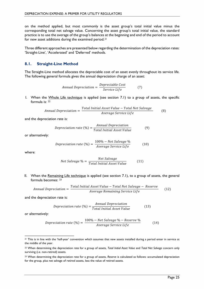
The Straight-Line method allocates the depreciable cost of an asset evenly throughout its service life. The following general formula gives the annual depreciation charge of an asset:
𝐴𝐴𝐴𝐴𝐴𝐴𝐴𝐴𝐴𝐴𝐴𝐴 𝐷𝐷𝐷𝐷𝐷𝐷𝐷𝐷𝐷𝐷𝐷𝐷𝐷𝐷𝐴𝐴𝐷𝐷𝐷𝐷𝐷𝐷𝐴𝐴 = 𝐷𝐷𝐷𝐷𝐷𝐷𝐷𝐷𝐷𝐷𝐷𝐷𝐷𝐷𝐴𝐴𝑏𝑏𝐴𝐴𝐷𝐷 𝐶𝐶𝐷𝐷𝐴𝐴𝐷𝐷𝑆𝑆𝐷𝐷𝐷𝐷𝑆𝑆𝐷𝐷𝐷𝐷𝐷𝐷 𝐿𝐿𝐷𝐷𝑜𝑜𝐷𝐷
(7)
I. When the Whole Life technique is applied (see section 7.1) to a group of assets, the specific formula is: 22
𝐴𝐴𝐴𝐴𝐴𝐴𝐴𝐴𝐴𝐴𝐴𝐴 𝐷𝐷𝐷𝐷𝐷𝐷𝐷𝐷𝐷𝐷𝐷𝐷𝐷𝐷𝐴𝐴𝐷𝐷𝐷𝐷𝐷𝐷𝐴𝐴 = 𝑇𝑇𝐷𝐷𝐷𝐷𝐴𝐴𝐴𝐴 𝐼𝐼𝐴𝐴𝐷𝐷𝐷𝐷𝐷𝐷𝐴𝐴𝐴𝐴 𝐴𝐴𝐴𝐴𝐴𝐴𝐷𝐷𝐷𝐷 𝑉𝑉𝐴𝐴𝐴𝐴𝐴𝐴𝐷𝐷 − 𝑇𝑇𝐷𝐷𝐷𝐷𝐴𝐴𝐴𝐴 𝑁𝑁𝐷𝐷𝐷𝐷 𝑆𝑆𝐴𝐴𝐴𝐴𝑆𝑆𝐴𝐴𝑆𝑆𝐷𝐷
𝐴𝐴𝑆𝑆𝐷𝐷𝐷𝐷𝐴𝐴𝑆𝑆𝐷𝐷 𝑆𝑆𝐷𝐷𝐷𝐷𝑆𝑆𝐷𝐷𝐷𝐷𝐷𝐷 𝐿𝐿𝐷𝐷𝑜𝑜𝐷𝐷 (8)
and the depreciation rate is:
𝐷𝐷𝐷𝐷𝐷𝐷𝐷𝐷𝐷𝐷𝐷𝐷𝐷𝐷𝐴𝐴𝐷𝐷𝐷𝐷𝐷𝐷𝐴𝐴 𝐷𝐷𝐴𝐴𝐷𝐷𝐷𝐷 (%) =𝐴𝐴𝐴𝐴𝐴𝐴𝐴𝐴𝐴𝐴𝐴𝐴 𝐷𝐷𝐷𝐷𝐷𝐷𝐷𝐷𝐷𝐷𝐷𝐷𝐷𝐷𝐴𝐴𝐷𝐷𝐷𝐷𝐷𝐷𝐴𝐴
𝑇𝑇𝐷𝐷𝐷𝐷𝐴𝐴𝐴𝐴 𝐼𝐼𝐴𝐴𝐷𝐷𝐷𝐷𝐷𝐷𝐴𝐴𝐴𝐴 𝐴𝐴𝐴𝐴𝐴𝐴𝐷𝐷𝐷𝐷 𝑉𝑉𝐴𝐴𝐴𝐴𝐴𝐴𝐷𝐷 (9)
or alternatively:
𝐷𝐷𝐷𝐷𝐷𝐷𝐷𝐷𝐷𝐷𝐷𝐷𝐷𝐷𝐴𝐴𝐷𝐷𝐷𝐷𝐷𝐷𝐴𝐴 𝐷𝐷𝐴𝐴𝐷𝐷𝐷𝐷 (%) = 100% − 𝑁𝑁𝐷𝐷𝐷𝐷 𝑆𝑆𝐴𝐴𝐴𝐴𝑆𝑆𝐴𝐴𝑆𝑆𝐷𝐷 %𝐴𝐴𝑆𝑆𝐷𝐷𝐷𝐷𝐴𝐴𝑆𝑆𝐷𝐷 𝑆𝑆𝐷𝐷𝐷𝐷𝑆𝑆𝐷𝐷𝐷𝐷𝐷𝐷 𝐿𝐿𝐷𝐷𝑜𝑜𝐷𝐷
(10)
where:
𝑁𝑁𝐷𝐷𝐷𝐷 𝑆𝑆𝐴𝐴𝐴𝐴𝑆𝑆𝐴𝐴𝑆𝑆𝐷𝐷 % = 𝑁𝑁𝐷𝐷𝐷𝐷 𝑆𝑆𝐴𝐴𝐴𝐴𝑆𝑆𝐴𝐴𝑆𝑆𝐷𝐷
𝑇𝑇𝐷𝐷𝐷𝐷𝐴𝐴𝐴𝐴 𝐼𝐼𝐴𝐴𝐷𝐷𝐷𝐷𝐷𝐷𝐴𝐴𝐴𝐴 𝐴𝐴𝐴𝐴𝐴𝐴𝐷𝐷𝐷𝐷 𝑉𝑉𝐴𝐴𝐴𝐴𝐴𝐴𝐷𝐷 (11)
II. When the Remaining Life technique is applied (see section 7.1), to a group of assets, the general formula becomes: 23
𝐴𝐴𝐴𝐴𝐴𝐴𝐴𝐴𝐴𝐴𝐴𝐴 𝐷𝐷𝐷𝐷𝐷𝐷𝐷𝐷𝐷𝐷𝐷𝐷𝐷𝐷𝐴𝐴𝐷𝐷𝐷𝐷𝐷𝐷𝐴𝐴 = 𝑇𝑇𝐷𝐷𝐷𝐷𝐴𝐴𝐴𝐴 𝐼𝐼𝐴𝐴𝐷𝐷𝐷𝐷𝐷𝐷𝐴𝐴𝐴𝐴 𝐴𝐴𝐴𝐴𝐴𝐴𝐷𝐷𝐷𝐷 𝑉𝑉𝐴𝐴𝐴𝐴𝐴𝐴𝐷𝐷 − 𝑇𝑇𝐷𝐷𝐷𝐷𝐴𝐴𝐴𝐴 𝑁𝑁𝐷𝐷𝐷𝐷 𝑆𝑆𝐴𝐴𝐴𝐴𝑆𝑆𝐴𝐴𝑆𝑆𝐷𝐷 − 𝑅𝑅𝐷𝐷𝐴𝐴𝐷𝐷𝐷𝐷𝑆𝑆𝐷𝐷
𝐴𝐴𝑆𝑆𝐷𝐷𝐷𝐷𝐴𝐴𝑆𝑆𝐷𝐷 𝑅𝑅𝐷𝐷𝑅𝑅𝐴𝐴𝐷𝐷𝐴𝐴𝐷𝐷𝐴𝐴𝑆𝑆 𝑆𝑆𝐷𝐷𝐷𝐷𝑆𝑆𝐷𝐷𝐷𝐷𝐷𝐷 𝐿𝐿𝐷𝐷𝑜𝑜𝐷𝐷 (12)
and the depreciation rate is:
𝐷𝐷𝐷𝐷𝐷𝐷𝐷𝐷𝐷𝐷𝐷𝐷𝐷𝐷𝐴𝐴𝐷𝐷𝐷𝐷𝐷𝐷𝐴𝐴 𝐷𝐷𝐴𝐴𝐷𝐷𝐷𝐷 (%) =𝐴𝐴𝐴𝐴𝐴𝐴𝐴𝐴𝐴𝐴𝐴𝐴 𝐷𝐷𝐷𝐷𝐷𝐷𝐷𝐷𝐷𝐷𝐷𝐷𝐷𝐷𝐴𝐴𝐷𝐷𝐷𝐷𝐷𝐷𝐴𝐴
𝑇𝑇𝐷𝐷𝐷𝐷𝐴𝐴𝐴𝐴 𝐼𝐼𝐴𝐴𝐷𝐷𝐷𝐷𝐷𝐷𝐴𝐴𝐴𝐴 𝐴𝐴𝐴𝐴𝐴𝐴𝐷𝐷𝐷𝐷 𝑉𝑉𝐴𝐴𝐴𝐴𝐴𝐴𝐷𝐷 (13)
or alternatively:
𝐷𝐷𝐷𝐷𝐷𝐷𝐷𝐷𝐷𝐷𝐷𝐷𝐷𝐷𝐴𝐴𝐷𝐷𝐷𝐷𝐷𝐷𝐴𝐴 𝐷𝐷𝐴𝐴𝐷𝐷𝐷𝐷 (%) = 100% − 𝑁𝑁𝐷𝐷𝐷𝐷 𝑆𝑆𝐴𝐴𝐴𝐴𝑆𝑆𝐴𝐴𝑆𝑆𝐷𝐷 % − 𝑅𝑅𝐷𝐷𝐴𝐴𝐷𝐷𝐷𝐷𝑆𝑆𝐷𝐷 %
𝐴𝐴𝑆𝑆𝐷𝐷𝐷𝐷𝐴𝐴𝑆𝑆𝐷𝐷 𝑆𝑆𝐷𝐷𝐷𝐷𝑆𝑆𝐷𝐷𝐷𝐷𝐷𝐷 𝐿𝐿𝐷𝐷𝑜𝑜𝐷𝐷 (14)
21 This is in line with the ‘half-year’ convention which assumes that new assets installed during a period enter in service at the middle of the year. 22 When determining the depreciation rate for a group of assets, Total Initial Asset Value and Total Net Salvage concern only surviving (i.e. non-retired) assets. 23 When determining the depreciation rate for a group of assets, Reserve is calculated as follows: accumulated depreciation for the group, plus net salvage of retired assets, less the value of retired assets.
DEPRECIATION EXPENSE: A PRIMER FOR UTILITY REGULATORS
Page 26
where
𝑅𝑅𝐷𝐷𝐴𝐴𝐷𝐷𝐷𝐷𝑆𝑆𝐷𝐷 % = 𝑅𝑅𝐷𝐷𝐴𝐴𝐷𝐷𝐷𝐷𝑆𝑆𝐷𝐷
𝑇𝑇𝐷𝐷𝐷𝐷𝐴𝐴𝐴𝐴 𝐼𝐼𝐴𝐴𝐷𝐷𝐷𝐷𝐷𝐷𝐴𝐴𝐴𝐴 𝐴𝐴𝐴𝐴𝐴𝐴𝐷𝐷𝐷𝐷 𝑉𝑉𝐴𝐴𝐴𝐴𝐴𝐴𝐷𝐷 (15)
Unless there is a reassessment of key input values, leading to a correction in the respective measure of average life (average service life or remaining service life) or in the net salvage, both techniques under the Straight-Line method result in constant depreciation rates and annual depreciation expense.
8.2. Accelerated Methods
Accelerated methods include approaches (‘Sum-of-the-Years-Digits’ and ‘Declining Balance’ methods) that result in higher depreciation expenses for the earlier years of the service life of an asset.24 The key advantage of Accelerated methods is that, in case estimates of service life are subject to wide possible error, only a small allocation of the initial asset value is left to the period near the end of an asset’ life.
Sum-of-the-Years-Digits method In the Sum-of-the-Years-Digits method, the rate varies with age resulting in higher charges in early service life and lower in later life. The initial value of the asset is fully recovered by the end of the asset’s life (in contrast to the Declining Balance method as discussed below). The depreciation rate in the asset’s year of age n is calculated as follows:
𝐷𝐷𝐷𝐷𝐷𝐷𝐷𝐷𝐷𝐷𝐷𝐷𝐷𝐷𝐴𝐴𝐷𝐷𝐷𝐷𝐷𝐷𝐴𝐴 𝐷𝐷𝐴𝐴𝐷𝐷𝐷𝐷𝑛𝑛(%) = 𝐿𝐿 − 𝐴𝐴 + 1∑ 𝑚𝑚𝐿𝐿1
× (100% −𝑁𝑁𝐷𝐷𝐷𝐷 𝑆𝑆𝐴𝐴𝐴𝐴𝑆𝑆𝐴𝐴𝑆𝑆𝐷𝐷 %) (16)
where: L is a measure of the asset’s life, ∑ 𝑚𝑚𝐿𝐿1 is the sum of each whole number from 1 to L.
The Sum-of-the-Years-Digits method results in an annual depreciation expense that decreases by a fixed amount each year along a straight line having a negative slope. The major drawback of this method is that it does not represent the true consumption pattern of assets.
If used with respect to a group of assets, the Sum-of-the-Years-Digits method must be applied separately for each vintage group (i.e. assets of a particular vintage) so that a changing depreciation rate can be applied to the vintage as it ages.
Declining Balance method
In the Declining Balance method, the depreciation rate is constant, but it is applied to the net asset balance instead of the gross asset balance. The depreciation rate is set higher than the rate estimated through the Straight-Line method by a factor of 1.5 or 2. In the ‘Double Declining’ method, for instance, the depreciation rate and expenses for a group of assets are given by the following formulas:
𝐷𝐷𝐷𝐷𝐷𝐷𝐷𝐷𝐷𝐷𝐷𝐷𝐷𝐷𝐴𝐴𝐷𝐷𝐷𝐷𝐷𝐷𝐴𝐴 𝐷𝐷𝐴𝐴𝐷𝐷𝐷𝐷 (%) = 2 ×100% − 𝑁𝑁𝐷𝐷𝐷𝐷 𝑆𝑆𝐴𝐴𝐴𝐴𝑆𝑆𝐴𝐴𝑆𝑆𝐷𝐷 (%)𝐴𝐴𝑆𝑆𝐷𝐷𝐷𝐷𝐴𝐴𝑆𝑆𝐷𝐷 𝑆𝑆𝐷𝐷𝐷𝐷𝑆𝑆𝐷𝐷𝐷𝐷𝐷𝐷 𝐿𝐿𝐷𝐷𝑜𝑜𝐷𝐷
(17)
𝐷𝐷𝐷𝐷𝐷𝐷𝐷𝐷𝐷𝐷𝐷𝐷𝐷𝐷𝐴𝐴𝐷𝐷𝐷𝐷𝐷𝐷𝐴𝐴 = 𝐷𝐷𝐷𝐷𝐷𝐷𝐷𝐷𝐷𝐷𝐷𝐷𝐷𝐷𝐴𝐴𝐷𝐷𝐷𝐷𝐷𝐷𝐴𝐴 𝐷𝐷𝐴𝐴𝐷𝐷𝐷𝐷 (%) × (𝑇𝑇𝐷𝐷𝐷𝐷𝐴𝐴𝐴𝐴 𝐼𝐼𝐴𝐴𝐷𝐷𝐷𝐷𝐷𝐷𝐴𝐴𝐴𝐴 𝐴𝐴𝐴𝐴𝐴𝐴𝐷𝐷𝐷𝐷 𝑉𝑉𝐴𝐴𝐴𝐴𝐴𝐴𝐷𝐷 − 𝑅𝑅𝐷𝐷𝐴𝐴𝐷𝐷𝐷𝐷𝑆𝑆𝐷𝐷) (18)
24 In case that a regulated entity uses the Accelerated depreciation for statutory (i.e. income tax) purposes and another method (i.e. the Straight-Line method) for regulatory purposes, there will be a difference between the regulatory and tax depreciation expenses, which complicates the utility’s bookkeeping.
DEPRECIATION EXPENSE: A PRIMER FOR UTILITY REGULATORS
Page 27
The major drawbacks of the Declining Balance method is that it may produce unwanted fluctuations in the annual depreciation expense and that, as in the Sum-of-the-Years-Digits method, it does not represent the true consumption pattern of assets. Additionally, the depreciation expense of each year decreases with age along a logarithmic curve, thus for depreciation expense close to zero the curve becomes asymptotic and the depreciable cost of the asset is never fully allocated. On the other hand, the Declining Balance method generates more internal funds from depreciation expenses (compared to the Straight-Line method) as long as overall gross asset value continues to grow.
8.3. Deferred Methods
Deferred methods include depreciation approaches that result in depreciation costs being deferred to the later years of the service life of an asset. In the deferred methods, besides the depreciation rate used, an interest rate is added. The most common deferred method is the ‘Sinking Fund’ method.
Sinking Fund Method The Sinking Fund method considers not only the investment cost of the asset, but also the opportunity cost of the investment in terms of the interest that could have been earned if the amount spent on purchasing the asset was invested elsewhere.
The depreciation rate in the Sinking Fund method is determined so that, when applied annually over the asset’s service life and coupled with interest credits to the reserve at the selected interest rate, it will cover the full cost of an asset. The basic formulas for the depreciation rate and the depreciation expense are the following:
𝐷𝐷𝐷𝐷𝐷𝐷𝐷𝐷𝐷𝐷𝐷𝐷𝐷𝐷𝐴𝐴𝐷𝐷𝐷𝐷𝐷𝐷𝐴𝐴 𝐷𝐷𝐴𝐴𝐷𝐷𝐷𝐷 (%) = (1 − 𝑁𝑁𝐷𝐷𝐷𝐷 𝑆𝑆𝐴𝐴𝐴𝐴𝑆𝑆𝐴𝐴𝑆𝑆𝐷𝐷 %) ×𝐷𝐷
(1 + 𝐷𝐷)𝐿𝐿 − 1 (19)
𝐷𝐷𝐷𝐷𝐷𝐷𝐷𝐷𝐷𝐷𝐷𝐷𝐷𝐷𝐴𝐴𝐷𝐷𝐷𝐷𝐷𝐷𝐴𝐴 = (𝐷𝐷𝐷𝐷𝐷𝐷𝐷𝐷𝐷𝐷𝐷𝐷𝐷𝐷𝐴𝐴𝐷𝐷𝐷𝐷𝐷𝐷𝐴𝐴 𝐷𝐷𝐴𝐴𝐷𝐷𝐷𝐷 × 𝑇𝑇𝐷𝐷𝐷𝐷𝐴𝐴𝐴𝐴 𝐼𝐼𝐴𝐴𝐷𝐷𝐷𝐷𝐷𝐷𝐴𝐴𝐴𝐴 𝐴𝐴𝐴𝐴𝐴𝐴𝐷𝐷𝐷𝐷 𝑉𝑉𝐴𝐴𝐴𝐴𝐴𝐴𝐷𝐷) + (𝐷𝐷 × 𝑅𝑅𝐷𝐷𝐴𝐴𝐷𝐷𝐷𝐷𝑆𝑆𝐷𝐷) (20)
where: L is a measure of the asset’s life 𝐷𝐷 is the net interest rate25 Compared to the Straight-Line method, the Sinking Fund method produces lower early depreciation expenses and higher expenses in the later years, due to the interest received on the accumulated depreciation reserve which increases as the asset ages. A major drawback of the Sinking Fund approach is that, due to the increasing interest towards the end of the asset’s service life, even when an asset is retired only one or two years earlier than the initially estimated time, a significant difference may arise between the accumulated depreciation and the cost being recovered (i.e. the total initial asset value). Thus, Deferred Methods require higher accuracy in the calculation of the average service life and net salvage of an asset group.26
8.4. Selection of Depreciation Rate
Concerning the selection of the appropriate type of depreciation rate, NARUC (1996, p.61) states:
The straight-line method is almost universally used in the utility rate making process. (…)
25 The Sinking Fund method can be also applied using the Remaining Life technique with equivalent formulas. 26 If the interest rate used in the Sinking Fund method is the same as the allowed rate of return on RAB (e.g. WACC), the method produces a constant total of depreciation expense and return each accounting period.
DEPRECIATION EXPENSE: A PRIMER FOR UTILITY REGULATORS
Page 28
The accelerated methods identified above are not generally used for regulatory purposes. (…)
Interest methods, such as the sinking fund method, are no longer in general use.
On the other hand, Pardina et al. (2008) note that Accelerated methods can be used for eliminating the risk of an asset’s underutilization or obsolescence.27 The usage of the Accelerated method may be appropriate in contexts such as the current one, where energy markets are evolving rapidly. Higher distributed generation and storage in the near future can provide network users with the option to bypass the grid fully or partially. If the Straight-Line method is used, future consumers may be required to pay for an asset which they do not benefit from. On the other hand, Accelerated methods may lead to overinvestments and replacement of assets that continue to provide useful services. In other words, if the asset is depreciated in the early years of its service life, then the utility might not have an incentive to maintain the asset but rather re-invest in asset replacements.
9. Asset Grouping
The final element of a depreciation system is the Procedure, or in other words the approach towards grouping of individual asset units (e.g. in Broad, Vintage or Equal Life group), which corresponds to the level at which the life characteristics and salvage values of assets are estimated through appropriate depreciation studies. The average service lives and corresponding depreciation rates of each group are then weighted to calculate the depreciation rate as well as the depreciation expense for each Account of the regulated entity. As noted by NARUC (1996, p. 20):
Generally speaking, smaller groups yield more accuracy, but there are diminishing returns because more detailed accounting records are required.
9.1. Grouping Approaches
The main grouping alternatives concerning the level at which the life characteristics and salvage values of assets are estimated, for the purpose of determining average service lives and corresponding depreciation rates, and then combined in order to determine the weighted average depreciation rate of account) are:
• Single Unit: Each unit is depreciated separately. Because the Procedure requires separate record-keeping for each unit, it is not practical for most types of assets, unless it concerns unique and stand-alone assets of significant value (e.g. generation stations).
• Broad Group: Grouped together units that have similar characteristics, are used in the same way and operate under the same conditions. These units are depreciated as a single group with a common average service life. Because of the averaging effect across assets in the Broad Group, this Procedure results in reasonably stable depreciation charges over time and is widely used.
This Procedure requires that at least accounting records of annual asset additions and balances are maintained. Retirements by vintage and associated estimation of the Broad Group’s survivor curve are desirable but not necessary. The Broad Group model views the asset group as a collection of vintages that each have the same characteristics, thus a single Initial Asset Value and a single Net Salvage are used to describe all assets in a Broad Group. An account may consist of one or more Broad Groups.
27 Pardina, Martin Rodriguez, Richard Schlirf Rapti, and Eric Groom. 2008. Accounting for Infrastructure Regulation. Washington:
The World Bank.
DEPRECIATION EXPENSE: A PRIMER FOR UTILITY REGULATORS
Page 29
• Vintage Group: groups together the units placed in service during the same year (i.e. each vintage is a separate group). In this Procedure, the depreciation characteristics and the average service life are analyzed separately for each vintage, and then all vintages are combined to determine the average service life of the account. The Vintage Group model views the account as a collection of vintage groups that may have different life and salvage characteristics. The major drawback of the Vintage Group Procedure is that because assets within a vintage may have very different life characteristics, many assets will be depreciated over a significantly longer or shorter timeframe than their actual service life.
Assets with shorter service lives than the vintage group average are under-depreciated, and assets with longer service lives than the group average are over-depreciated. Therefore, the Procedure does not send the right signal when the retirement of an asset occurs as over-accumulation or under-accumulation of depreciation will arise over time. The Equal Life Group Procedure addresses this issue. Nevertheless, in the longer term, both Procedures result in the same total accumulated depreciation expenses for the account and the assets are fully recovered by the time all assets of a vintage are depreciated.
• Equal Life Group: groups together assets within vintage groups that have similar life characteristics and the same expected service life. In other words, each vintage group within the account is divided into smaller sub-groups, each of which is limited to units that are expected to have the same life, and depreciates them over the group’s average service life. The depreciation rate is calculated separately for the Equal Life Groups before being combined to determine the total depreciation of the account. Through this Procedure, the full cost of the shorter-lived units is fully depreciated while they are in service and thus the longer-lived units bear only their own costs. Both the Vintage Group and the Equal Life Procedures require that survivor curves are available. For the Equal Life Group in particular, the survivor curves are required to determine the subgroups within the vintage groups. Even though the Equal Life Group is preferable to the Vintage Group Procedures, it is still expected to produce greater fluctuations in depreciation expense from year to year than the Broad Group Procedure.
9.2. Group Weighting
When groups are defined and their average service lives as well as associated depreciation rates are estimated, these groups need to be combined (through appropriate weighting) to determine the depreciation rate for the account. Weighting is important, as the average service life (and thus the depreciation rate) of an account changes according to the changing composition of its component groups.
Direct weighting
Direct weighting is presented in this section for illustrative purposes and it is not appropriate for weighting different groups (e.g. Vintage Groups or Equal Life Groups). Given two units, which start their operation in the same year, their investment cost is €100 each, the salvage is zero, and their service lives are five and 10 years, their direct weighted average life equals 7.5 years and the depreciation rate (using the Straight-Line method) is 13.33%. For the first five years, the depreciation each year is €200 (total Initial Asset Value) multiplied by the 13.33% rate. In other words, by the end of the first five years, €133.33 will have been depreciated. For the next 5 years, only one unit remains and the depreciation each year is €100 multiplied by the 13.33% rate. In this way, by the end of the 10th year, the investment cost of €200 is completely depreciated.
DEPRECIATION EXPENSE: A PRIMER FOR UTILITY REGULATORS
Page 30
Reciprocal (harmonic) weighting
Reciprocal (harmonic) weighting is the appropriate approach for weighting Vintage Groups and Equal Life Groups (and also Broad Groups if more than one is specified within an account) for the purpose of determining the depreciation rate of the account. Consider the above example with respect to groups of assets, instead of units. The first group (A) has a five-year average service life and an Initial Asset Value of €100, while the second group (B) has a 10-year average service life and an Initial Asset Value of €300. The method of reciprocal weighting is: During the first 5 years, the reciprocal weighted average service life (RWASL) is:
𝑅𝑅𝑅𝑅𝐴𝐴𝑆𝑆𝐿𝐿 = 𝑇𝑇𝐷𝐷𝐷𝐷𝐴𝐴𝐴𝐴 𝐼𝐼𝐴𝐴𝐷𝐷𝐷𝐷𝐷𝐷𝐴𝐴𝐴𝐴 𝐴𝐴𝐴𝐴𝐴𝐴𝐷𝐷𝐷𝐷 𝑉𝑉𝐴𝐴𝐴𝐴𝐴𝐴𝐷𝐷 ÷ �𝐼𝐼𝐴𝐴𝐷𝐷𝐷𝐷𝐷𝐷𝐴𝐴𝐴𝐴 𝐴𝐴𝐴𝐴𝐴𝐴𝐷𝐷𝐷𝐷 𝑉𝑉𝐴𝐴𝐴𝐴𝐴𝐴𝐷𝐷 𝐴𝐴𝐴𝐴𝑆𝑆𝐷𝐷𝐷𝐷𝐴𝐴𝑆𝑆𝐷𝐷 𝑆𝑆𝐷𝐷𝐷𝐷𝑆𝑆𝐷𝐷𝐷𝐷𝐷𝐷 𝐿𝐿𝐷𝐷𝑜𝑜𝐷𝐷 𝐴𝐴
+ 𝐼𝐼𝐴𝐴𝐷𝐷𝐷𝐷𝐷𝐷𝐴𝐴𝐴𝐴 𝐴𝐴𝐴𝐴𝐴𝐴𝐷𝐷𝐷𝐷 𝑉𝑉𝐴𝐴𝐴𝐴𝐴𝐴𝐷𝐷 𝐵𝐵𝐴𝐴𝑆𝑆𝐷𝐷𝐷𝐷𝐴𝐴𝑆𝑆𝐷𝐷 𝑆𝑆𝐷𝐷𝐷𝐷𝑆𝑆𝐷𝐷𝐷𝐷𝐷𝐷 𝐿𝐿𝐷𝐷𝑜𝑜𝐷𝐷 𝐵𝐵
�
thus,
𝑅𝑅𝑅𝑅𝐴𝐴𝑆𝑆𝐿𝐿 = €400 ÷ (€20 + €30) = 8
and the corresponding depreciation rate is:
𝐷𝐷𝐷𝐷𝐷𝐷𝐷𝐷𝐷𝐷𝐷𝐷𝐷𝐷𝐴𝐴𝐷𝐷𝐷𝐷𝐷𝐷𝐴𝐴 𝑅𝑅𝐴𝐴𝐷𝐷𝐷𝐷 = 100%𝑅𝑅𝑅𝑅𝐴𝐴𝑆𝑆𝐿𝐿
= 12.5%
The accumulated depreciation for the first five years is thus:
𝐴𝐴𝐷𝐷𝐷𝐷𝐴𝐴𝑅𝑅𝐴𝐴𝐴𝐴𝐴𝐴𝐷𝐷𝐷𝐷𝑢𝑢 𝐷𝐷𝐷𝐷𝐷𝐷𝐷𝐷𝐷𝐷𝐷𝐷𝐷𝐷𝐴𝐴𝐷𝐷𝐷𝐷𝐷𝐷𝐴𝐴 𝑜𝑜𝐷𝐷𝐷𝐷 𝑜𝑜𝐷𝐷𝐷𝐷𝐴𝐴𝐷𝐷 𝑜𝑜𝐷𝐷𝑆𝑆𝐷𝐷 𝑌𝑌𝐷𝐷𝐴𝐴𝐷𝐷𝐴𝐴 = 5 × (12.5% × €400) = €250
In the remaining five years of service of group B, the reserve of €150 is depreciated at a rate of:
𝐷𝐷𝐷𝐷𝐷𝐷𝐷𝐷𝐷𝐷𝐷𝐷𝐷𝐷𝐴𝐴𝐷𝐷𝐷𝐷𝐷𝐷𝐴𝐴 𝑅𝑅𝐴𝐴𝐷𝐷𝐷𝐷 = 100%
𝐴𝐴𝑆𝑆𝐷𝐷𝐷𝐷𝐴𝐴𝑆𝑆𝐷𝐷 𝑆𝑆𝐷𝐷𝐷𝐷𝑆𝑆𝐷𝐷𝐷𝐷𝐷𝐷 𝐿𝐿𝐷𝐷𝑜𝑜𝐷𝐷 𝐵𝐵= 10%
and the accumulated depreciation for the remaining five years is thus:
𝐴𝐴𝐷𝐷𝐷𝐷𝐴𝐴𝑅𝑅𝐴𝐴𝐴𝐴𝐴𝐴𝐷𝐷𝐷𝐷𝑢𝑢 𝐷𝐷𝐷𝐷𝐷𝐷𝐷𝐷𝐷𝐷𝐷𝐷𝐷𝐷𝐴𝐴𝐷𝐷𝐷𝐷𝐷𝐷𝐴𝐴 𝑜𝑜𝐷𝐷𝐷𝐷 𝐴𝐴𝐴𝐴𝐴𝐴𝐷𝐷 𝑜𝑜𝐷𝐷𝑆𝑆𝐷𝐷 𝑌𝑌𝐷𝐷𝐴𝐴𝐷𝐷𝐴𝐴 = 5 × (10% × €300) = €150
Therefore, the Total Initial Asset Value of €400 is fully depreciated by the end of the 10th year.
10. Regulatory Considerations
Regulatory depreciation is an important issue for the regulator, for several reasons:
• Regulated activities are usually capital intensive; thus, depreciation is a major component of the costs that need to be recovered through tariffs.
• There is a wide range of alternative approaches concerning the determination of depreciation expenses so the regulator, depending on priorities, is able to choose between smoothing regulated prices and normalizing cash flows (e.g. through Straight-Line Method and Broad Group Procedure), or reducing risks for the regulated entity associated with technological or demand-related obsolescence (e.g. through the Accelerated Method).
DEPRECIATION EXPENSE: A PRIMER FOR UTILITY REGULATORS
Page 31
• Revisions or adjustments in key input for determining depreciation expense may result in significant windfall gains or losses (e.g. following re-valuation of assets through replacement costs) for the regulated entity, and even in assets becoming stranded.28
For this reason, regulators need to develop their monitoring skills. They must understand the potential risks for the regulated business and identify associated treatments and opportunities, in order to ensure delivery of the required services and recovery of the capital invested. Emerging energy technologies such as renewable sources (especially small-scale distributed sources) and energy storage systems, may significantly affect the development of transmission and distribution networks, causing investment deferrals in both networks. Additionally, the advent of such technologies, by reducing the net demand to be supplied through transmission and distribution networks, may lead to (partial) stranding of existing networks. Stranding, to the extent that it characterizes only a lower than expected utilization of the asset (and not also a non-recognition of associated costs by the regulator) is expected to affect (negatively) the prices that consumers have to pay for network services, since customers will be required to pay for non-efficiently incurred investments, or in other words investments which are no longer associated with the true economic cost of providing the regulated service. To the extent that stranding is also associated with non-recognition of associated costs by the regulator, the corresponding risk is expected to be reflected a priori in the regulated entity’s financing costs and thus on tariffs. Thus, more favorable conditions may need to be provided by the regulator to network companies in order to mitigate this risk and limit financing costs. Such conditions may include the use of Accelerated rather than Straight-Line depreciation Method or greater flexibility in the recognition of investment costs, to encourage utilities to make long-term investments in network assets.29 In particular, the Accelerated Method of depreciation, by allowing greater depreciation expenses in the early years of the life of an asset, reduces the risks of investment recovery that are associated with a longer period. Greater flexibility in the recognition of investment costs and of associated depreciation expenses can lead to smoother tariffs at times when other cost elements, such as the cost of capital, are low.30 On the other hand, Accelerated depreciation methods create instability in tariffs, as the cost of depreciation and thus prices would tend to be higher in the early years of the asset’s life and decrease in the long term as the asset ages. Moreover, as depreciation is one of the main building blocks of Allowed Revenue, the Accelerated Method may remove an asset owner’s incentive to continue to use the asset once it is fully depreciated. Once the asset is fully depreciated, the utility only earns revenue from associated operational expenses as neither depreciation nor return on the asset apply. In such a case, the utility may not have an incentive to properly maintain assets and may aim to replace the depreciated assets even if it remains fully functional.
28 Stranded assets are commonly defined as those assets which, at some time prior to the end of their service life, as a result of changes in market and regulatory conditions, are not utilized to the level originally foreseen for the purpose of providing the regulated service, and are thus expected to be unable to fully recover their cost. 29 Such regulatory measures aimed at ensuring the financial sustainability of investments should ensure that the asset value to be recovered through depreciation corresponds to a representative measure of asset costs. The main aspect to be adjusted by the regulator concerns the time schedule of this recovery. 30 In order to adhere to the principle of economic efficiency, such adjustments in the recognized depreciation expenses should be made only when the asset’s utilization rates deviate from the expected (e.g. as a result of higher than expected demand).
DEPRECIATION EXPENSE: A PRIMER FOR UTILITY REGULATORS
Page 32
11. Final Remarks
The development and application of cost-reflective tariffs, based on sound economic principles, is of crucial importance for safeguarding the financial viability of energy utilities and of the electricity sector as a whole, as well as for ensuring that appropriate incentives are in place for attracting necessary investments in the sector.
This primer presents key factors affecting allowed depreciation costs, as well as alternative approaches and regulatory considerations that may be useful when determining allowed depreciation. Utilizing these approaches in combination with informed judgment is beneficial to utilities, investors, and customers.
DEPRECIATION EXPENSE: A PRIMER FOR UTILITY REGULATORS
Page 33
Annex I: Numerical Example
In this Annex, a numerical example is presented, applying the approaches and formulas described in sections 7.2 (‘Estimating Service Life’) and 8 (‘Depreciation Rate’). The respective formulas in the main sections of the Primer are indexed for ease of reference.
Estimating Service Life
As discussed in section 7.2, when statistical historical data on the age of each asset (i.e. aged data) is available, the mortality characteristics of asset groups (i.e. the age at which assets within a certain group retire) can be analyzed using actuarial methods. Actuarial methods produce the survivor curves required for estimating the average life and the average remaining life of assets in a group. In this fictitious example, we assume that a detailed historical record of the age of each asset within a group is available, from the date of installation to the date of retirement. The assets we examine concern a Broad Group (see section 9.2 for a discussion of ‘Grouping Approaches’), in other words a group of units that have similar characteristics, are used in the same way and operate under the same conditions (e.g. poles). Through this analysis, the objective is to produce the observed survivor curve for this particular category of assets. The survivor curve will be used to estimate the average service life (or the average remaining service life) and the depreciation rate that should be applied to assets belonging in this category. Based on the statistical historical data available, the total initial value of the assets in this category (placed in service at various years) is calculated at $1,000,000. The observed value of retirements occurring at each age interval (x) is shown in column 3 of Table 1. The value of assets surviving at the end of each year is shown in column 2. The retirement rate (rrx) at each age interval is shown in column 4 and is calculated according to formula (5) of Section 7.2, using the values of column 3 (Retirements) and column 2 (Surviving Assets):
𝐷𝐷𝐷𝐷𝑥𝑥 = 𝑅𝑅𝐷𝐷𝐷𝐷𝐷𝐷𝐷𝐷𝐷𝐷𝑅𝑅𝐷𝐷𝐴𝐴𝐷𝐷𝐴𝐴 𝑢𝑢𝐴𝐴𝐷𝐷𝐷𝐷𝐴𝐴𝑆𝑆 𝐴𝐴𝑆𝑆𝐷𝐷 𝐷𝐷𝐴𝐴𝐷𝐷𝐷𝐷𝐷𝐷𝑆𝑆𝐴𝐴𝐴𝐴 𝑚𝑚
𝐴𝐴𝐴𝐴𝐴𝐴𝐷𝐷𝐷𝐷𝐴𝐴 𝐴𝐴𝐴𝐴𝐷𝐷𝑆𝑆𝐷𝐷𝐴𝐴𝑆𝑆 𝐴𝐴𝐷𝐷 𝐷𝐷ℎ𝐷𝐷 𝑏𝑏𝐷𝐷𝑆𝑆𝐷𝐷𝐴𝐴𝐴𝐴𝐷𝐷𝐴𝐴𝑆𝑆 𝐷𝐷𝑜𝑜 𝐴𝐴𝑆𝑆𝐷𝐷 𝐷𝐷𝐴𝐴𝐷𝐷𝐷𝐷𝐷𝐷𝑆𝑆𝐴𝐴𝐴𝐴 𝑚𝑚
The percent of assets (Sx) surviving at the beginning of age interval x, is shown in column 6. It is estimated according to formula (6) of Section 7.2, using the values of column 4 (Retirement Rate) and starting from a value of 100% (i.e. all assets are surviving at the beginning of age interval 1):
𝑆𝑆𝑋𝑋+1 = 𝑆𝑆𝑋𝑋 − (𝐷𝐷𝐷𝐷𝑥𝑥 × 𝑆𝑆𝑋𝑋)
The survivor curve, depicting the percent of assets (Sx) surviving at each year of age is shown in Figure 1.
The average service life is estimated using formula (3) of Section 7.2:
𝐴𝐴𝑆𝑆𝐷𝐷𝐷𝐷𝐴𝐴𝑆𝑆𝐷𝐷 𝑆𝑆𝐷𝐷𝐷𝐷𝑆𝑆𝐷𝐷𝐷𝐷𝐷𝐷 𝐿𝐿𝐷𝐷𝑜𝑜𝐷𝐷 =𝐴𝐴𝐷𝐷𝐷𝐷𝐴𝐴 𝐴𝐴𝐴𝐴𝑢𝑢𝐷𝐷𝐷𝐷 𝑆𝑆𝐶𝐶 𝑜𝑜𝐷𝐷𝐷𝐷𝑅𝑅 𝐴𝐴𝑆𝑆𝐷𝐷 0 𝐷𝐷𝐷𝐷 𝑅𝑅𝐴𝐴𝑚𝑚
100%
The area under the survivor curve (SC) is estimated as the sum of the areas of all trapezoids between ages n-1 and n, as shown in Figure 1, from age 0 to maximum life. The area of a trapezoid between age n-1 and age n is presented in column 7 of Table 1 and is estimated using the following formula:
𝑇𝑇𝐷𝐷𝐴𝐴𝐷𝐷𝐷𝐷𝑇𝑇𝐷𝐷𝐷𝐷𝑢𝑢 𝐴𝐴𝐷𝐷𝐷𝐷𝐴𝐴 =𝑆𝑆𝑛𝑛−1 + 𝑆𝑆𝑛𝑛
2× [𝐴𝐴 − (𝐴𝐴 − 1)]
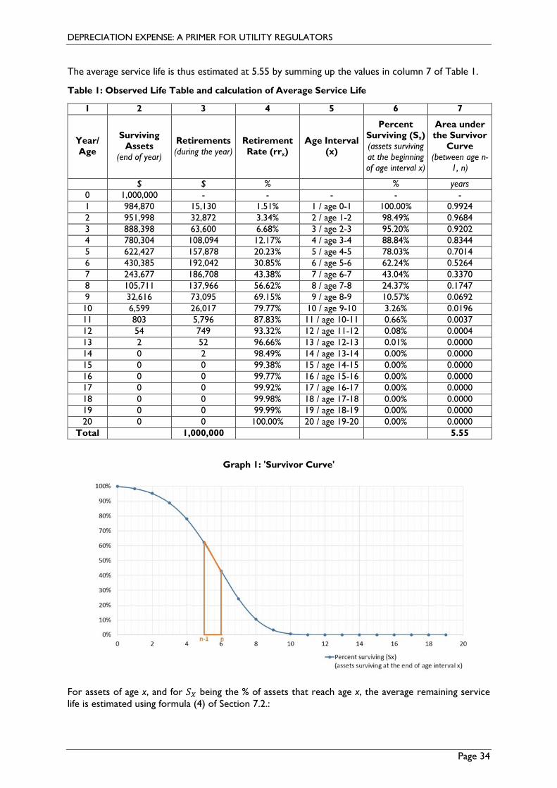
DEPRECIATION EXPENSE: A PRIMER FOR UTILITY REGULATORS
Page 34
The average service life is thus estimated at 5.55 by summing up the values in column 7 of Table 1.
Table 1: Observed Life Table and calculation of Average Service Life
1 2 3 4 5 6 7
Year/ Age
Surviving Assets
(end of year)
Retirements (during the year)
Retirement Rate (rrx)
Age Interval (x)
Percent Surviving (Sx) (assets surviving at the beginning of age interval x)
Area under the Survivor
Curve (between age n-
1, n)
$ $ % % years 0 1,000,000 - - - - - 1 984,870 15,130 1.51% 1 / age 0-1 100.00% 0.9924 2 951,998 32,872 3.34% 2 / age 1-2 98.49% 0.9684 3 888,398 63,600 6.68% 3 / age 2-3 95.20% 0.9202 4 780,304 108,094 12.17% 4 / age 3-4 88.84% 0.8344 5 622,427 157,878 20.23% 5 / age 4-5 78.03% 0.7014 6 430,385 192,042 30.85% 6 / age 5-6 62.24% 0.5264 7 243,677 186,708 43.38% 7 / age 6-7 43.04% 0.3370 8 105,711 137,966 56.62% 8 / age 7-8 24.37% 0.1747 9 32,616 73,095 69.15% 9 / age 8-9 10.57% 0.0692 10 6,599 26,017 79.77% 10 / age 9-10 3.26% 0.0196 11 803 5,796 87.83% 11 / age 10-11 0.66% 0.0037 12 54 749 93.32% 12 / age 11-12 0.08% 0.0004 13 2 52 96.66% 13 / age 12-13 0.01% 0.0000 14 0 2 98.49% 14 / age 13-14 0.00% 0.0000 15 0 0 99.38% 15 / age 14-15 0.00% 0.0000 16 0 0 99.77% 16 / age 15-16 0.00% 0.0000 17 0 0 99.92% 17 / age 16-17 0.00% 0.0000 18 0 0 99.98% 18 / age 17-18 0.00% 0.0000 19 0 0 99.99% 19 / age 18-19 0.00% 0.0000 20 0 0 100.00% 20 / age 19-20 0.00% 0.0000
Total 1,000,000 5.55
Graph 1: 'Survivor Curve'
For assets of age x, and for 𝑆𝑆𝑋𝑋 being the % of assets that reach age x, the average remaining service life is estimated using formula (4) of Section 7.2.:
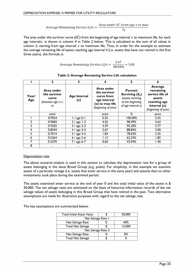
DEPRECIATION EXPENSE: A PRIMER FOR UTILITY REGULATORS
Page 35
𝐴𝐴𝑆𝑆𝐷𝐷𝐷𝐷𝐴𝐴𝑆𝑆𝐷𝐷 𝑅𝑅𝐷𝐷𝑅𝑅𝐴𝐴𝐷𝐷𝐴𝐴𝐷𝐷𝐴𝐴𝑆𝑆 𝑆𝑆𝐷𝐷𝐷𝐷𝑆𝑆𝐷𝐷𝐷𝐷𝐷𝐷 𝐿𝐿𝐷𝐷𝑜𝑜𝐷𝐷 = 𝐴𝐴𝐷𝐷𝐷𝐷𝐴𝐴 𝐴𝐴𝐴𝐴𝑢𝑢𝐷𝐷𝐷𝐷 𝑆𝑆𝐶𝐶 𝑜𝑜𝐷𝐷𝐷𝐷𝑅𝑅 𝐴𝐴𝑆𝑆𝐷𝐷 𝑚𝑚 𝐷𝐷𝐷𝐷 𝑅𝑅𝐴𝐴𝑚𝑚
𝑆𝑆𝑋𝑋
The area under the survivor curve (SC) from the beginning of age interval 𝑚𝑚 to maximum life, for each age interval𝑚𝑚, is shown in column 4 in Table 2 below. This is calculated as the sum of all values in column 2, starting from age interval 𝑚𝑚 to maximum life. Thus, in order for the example to estimate the average remaining life of assets reaching age interval 4 (i.e. assets that have not retired in the first three years), the formula is:
𝐴𝐴𝑆𝑆𝐷𝐷𝐷𝐷𝐴𝐴𝑆𝑆𝐷𝐷 𝑅𝑅𝐷𝐷𝑅𝑅𝐴𝐴𝐷𝐷𝐴𝐴𝐷𝐷𝐴𝐴𝑆𝑆 𝑆𝑆𝐷𝐷𝐷𝐷𝑆𝑆𝐷𝐷𝐷𝐷𝐷𝐷 𝐿𝐿𝐷𝐷𝑜𝑜𝐷𝐷 = 2.67
88.84%= 3.00
Table 2: Average Remaining Service Life calculation
1 2 3 4 5 6
Year/ Age
Area under the survivor
curve (between age n-1,
n)
Age Interval (x)
Area under the survivor curve from age interval
(x) to max life (beginning of year)
Percent Surviving (Sx) (assets surviving at the beginning of age interval x)
Average remaining
service life of assets
reaching age interval (x)
(beginning of year) years years % years 1 0.9924 1 / age 0-1 5.55 100.00% 5.55 2 0.9684 2 / age 1-2 4.56 98.49% 4.63 3 0.9202 3 / age 2-3 3.59 95.20% 3.77 4 0.8344 4 / age 3-4 2.67 88.84% 3.00 5 0.7014 5 / age 4-5 1.83 78.03% 2.35 6 0.5264 6 / age 5-6 1.13 62.24% 1.82 7 0.3370 7 / age 6-7 0.60 43.04% 1.40 8 … … … … …
Depreciation rate
The above actuarial analysis is used in this section to calculate the depreciation rate for a group of assets belonging in the same Broad Group (e.g. poles). For simplicity, in this example we examine assets of a particular vintage (i.e. assets that enter service in the same year) and assume that no other investments took place during the examined period. The assets examined enter service at the end of year 0 and the total initial value of the assets is $ 30,000. The net salvage rates are estimated on the basis of historical information records of the net salvage values of assets belonging in this Broad Group that have retired in the past. Two alternative assumptions are made for illustrative purposes with regard to the net salvage rate. The key assumptions are summarized below.
Total Initial Asset Value $ 30,000 Net Salvage Rate 1
Net Salvage Rate % 40% Total Net Salvage $ 12,000
Net Salvage Rate 2 Net Salvage Rate % 0% Total Net Salvage $ 0
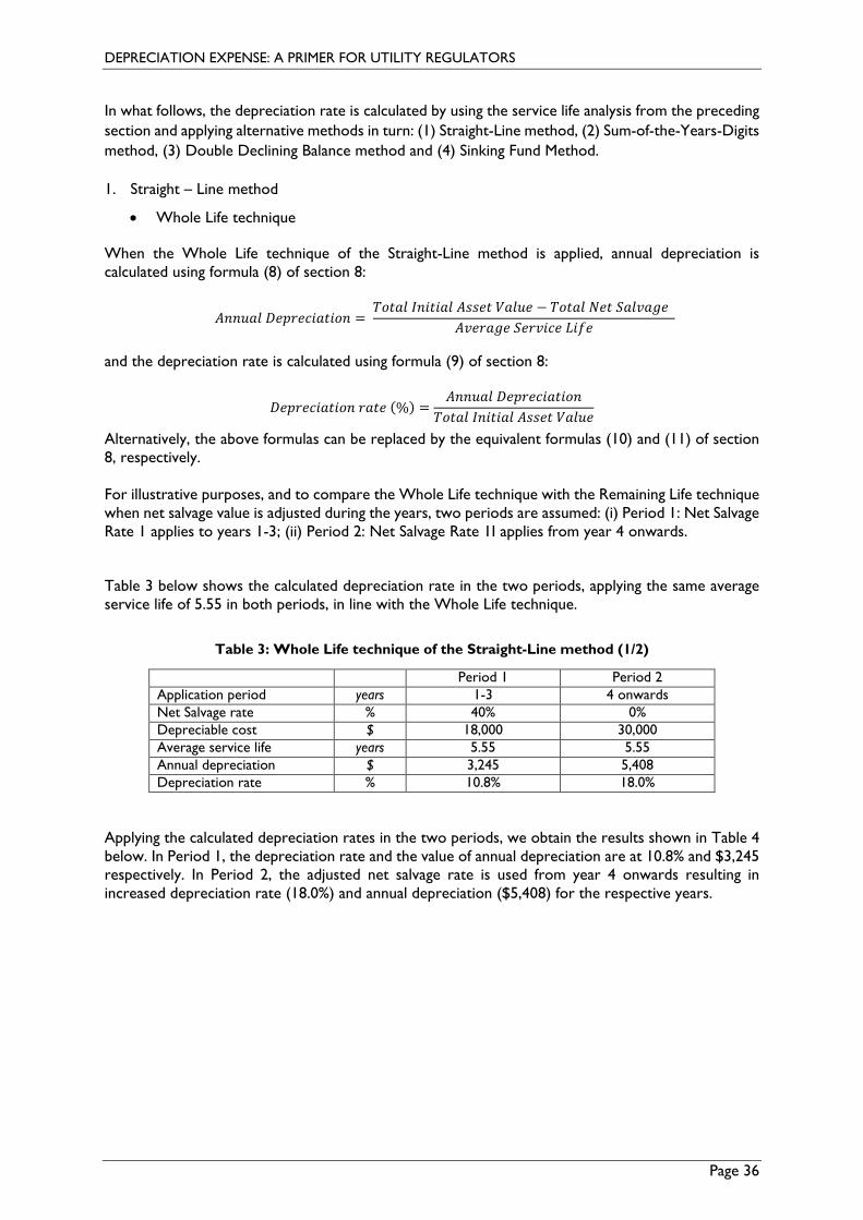
DEPRECIATION EXPENSE: A PRIMER FOR UTILITY REGULATORS
Page 36
In what follows, the depreciation rate is calculated by using the service life analysis from the preceding section and applying alternative methods in turn: (1) Straight-Line method, (2) Sum-of-the-Years-Digits method, (3) Double Declining Balance method and (4) Sinking Fund Method. 1. Straight – Line method
• Whole Life technique
When the Whole Life technique of the Straight-Line method is applied, annual depreciation is calculated using formula (8) of section 8:
𝐴𝐴𝐴𝐴𝐴𝐴𝐴𝐴𝐴𝐴𝐴𝐴 𝐷𝐷𝐷𝐷𝐷𝐷𝐷𝐷𝐷𝐷𝐷𝐷𝐷𝐷𝐴𝐴𝐷𝐷𝐷𝐷𝐷𝐷𝐴𝐴 = 𝑇𝑇𝐷𝐷𝐷𝐷𝐴𝐴𝐴𝐴 𝐼𝐼𝐴𝐴𝐷𝐷𝐷𝐷𝐷𝐷𝐴𝐴𝐴𝐴 𝐴𝐴𝐴𝐴𝐴𝐴𝐷𝐷𝐷𝐷 𝑉𝑉𝐴𝐴𝐴𝐴𝐴𝐴𝐷𝐷 − 𝑇𝑇𝐷𝐷𝐷𝐷𝐴𝐴𝐴𝐴 𝑁𝑁𝐷𝐷𝐷𝐷 𝑆𝑆𝐴𝐴𝐴𝐴𝑆𝑆𝐴𝐴𝑆𝑆𝐷𝐷
𝐴𝐴𝑆𝑆𝐷𝐷𝐷𝐷𝐴𝐴𝑆𝑆𝐷𝐷 𝑆𝑆𝐷𝐷𝐷𝐷𝑆𝑆𝐷𝐷𝐷𝐷𝐷𝐷 𝐿𝐿𝐷𝐷𝑜𝑜𝐷𝐷
and the depreciation rate is calculated using formula (9) of section 8:
𝐷𝐷𝐷𝐷𝐷𝐷𝐷𝐷𝐷𝐷𝐷𝐷𝐷𝐷𝐴𝐴𝐷𝐷𝐷𝐷𝐷𝐷𝐴𝐴 𝐷𝐷𝐴𝐴𝐷𝐷𝐷𝐷 (%) =𝐴𝐴𝐴𝐴𝐴𝐴𝐴𝐴𝐴𝐴𝐴𝐴 𝐷𝐷𝐷𝐷𝐷𝐷𝐷𝐷𝐷𝐷𝐷𝐷𝐷𝐷𝐴𝐴𝐷𝐷𝐷𝐷𝐷𝐷𝐴𝐴
𝑇𝑇𝐷𝐷𝐷𝐷𝐴𝐴𝐴𝐴 𝐼𝐼𝐴𝐴𝐷𝐷𝐷𝐷𝐷𝐷𝐴𝐴𝐴𝐴 𝐴𝐴𝐴𝐴𝐴𝐴𝐷𝐷𝐷𝐷 𝑉𝑉𝐴𝐴𝐴𝐴𝐴𝐴𝐷𝐷
Alternatively, the above formulas can be replaced by the equivalent formulas (10) and (11) of section 8, respectively. For illustrative purposes, and to compare the Whole Life technique with the Remaining Life technique when net salvage value is adjusted during the years, two periods are assumed: (i) Period 1: Net Salvage Rate 1 applies to years 1-3; (ii) Period 2: Net Salvage Rate 1I applies from year 4 onwards.
Table 3 below shows the calculated depreciation rate in the two periods, applying the same average service life of 5.55 in both periods, in line with the Whole Life technique.
Table 3: Whole Life technique of the Straight-Line method (1/2)
Period 1 Period 2 Application period years 1-3 4 onwards Net Salvage rate % 40% 0% Depreciable cost $ 18,000 30,000 Average service life years 5.55 5.55 Annual depreciation $ 3,245 5,408 Depreciation rate % 10.8% 18.0%
Applying the calculated depreciation rates in the two periods, we obtain the results shown in Table 4 below. In Period 1, the depreciation rate and the value of annual depreciation are at 10.8% and $3,245 respectively. In Period 2, the adjusted net salvage rate is used from year 4 onwards resulting in increased depreciation rate (18.0%) and annual depreciation ($5,408) for the respective years.
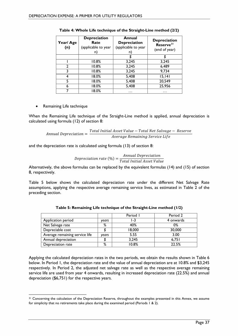
DEPRECIATION EXPENSE: A PRIMER FOR UTILITY REGULATORS
Page 37
Table 4: Whole Life technique of the Straight-Line method (2/2)
Year/ Age (n)
Depreciation Rate
(applicable to year n)
Annual Depreciation
(applicable to year n)
Depreciation Reserve31
(end of year)
$ $ 1 10.8% 3,245 3,245 2 10.8% 3,245 6,489 3 10.8% 3,245 9,734 4 18.0% 5,408 15,141 5 18.0% 5,408 20,549 6 18.0% 5,408 25,956 7 18.0% … …
• Remaining Life technique
When the Remaining Life technique of the Straight-Line method is applied, annual depreciation is calculated using formula (12) of section 8:
𝐴𝐴𝐴𝐴𝐴𝐴𝐴𝐴𝐴𝐴𝐴𝐴 𝐷𝐷𝐷𝐷𝐷𝐷𝐷𝐷𝐷𝐷𝐷𝐷𝐷𝐷𝐴𝐴𝐷𝐷𝐷𝐷𝐷𝐷𝐴𝐴 = 𝑇𝑇𝐷𝐷𝐷𝐷𝐴𝐴𝐴𝐴 𝐼𝐼𝐴𝐴𝐷𝐷𝐷𝐷𝐷𝐷𝐴𝐴𝐴𝐴 𝐴𝐴𝐴𝐴𝐴𝐴𝐷𝐷𝐷𝐷 𝑉𝑉𝐴𝐴𝐴𝐴𝐴𝐴𝐷𝐷 − 𝑇𝑇𝐷𝐷𝐷𝐷𝐴𝐴𝐴𝐴 𝑁𝑁𝐷𝐷𝐷𝐷 𝑆𝑆𝐴𝐴𝐴𝐴𝑆𝑆𝐴𝐴𝑆𝑆𝐷𝐷 − 𝑅𝑅𝐷𝐷𝐴𝐴𝐷𝐷𝐷𝐷𝑆𝑆𝐷𝐷
𝐴𝐴𝑆𝑆𝐷𝐷𝐷𝐷𝐴𝐴𝑆𝑆𝐷𝐷 𝑅𝑅𝐷𝐷𝑅𝑅𝐴𝐴𝐷𝐷𝐴𝐴𝐷𝐷𝐴𝐴𝑆𝑆 𝑆𝑆𝐷𝐷𝐷𝐷𝑆𝑆𝐷𝐷𝐷𝐷𝐷𝐷 𝐿𝐿𝐷𝐷𝑜𝑜𝐷𝐷
and the depreciation rate is calculated using formula (13) of section 8:
𝐷𝐷𝐷𝐷𝐷𝐷𝐷𝐷𝐷𝐷𝐷𝐷𝐷𝐷𝐴𝐴𝐷𝐷𝐷𝐷𝐷𝐷𝐴𝐴 𝐷𝐷𝐴𝐴𝐷𝐷𝐷𝐷 (%) =𝐴𝐴𝐴𝐴𝐴𝐴𝐴𝐴𝐴𝐴𝐴𝐴 𝐷𝐷𝐷𝐷𝐷𝐷𝐷𝐷𝐷𝐷𝐷𝐷𝐷𝐷𝐴𝐴𝐷𝐷𝐷𝐷𝐷𝐷𝐴𝐴
𝑇𝑇𝐷𝐷𝐷𝐷𝐴𝐴𝐴𝐴 𝐼𝐼𝐴𝐴𝐷𝐷𝐷𝐷𝐷𝐷𝐴𝐴𝐴𝐴 𝐴𝐴𝐴𝐴𝐴𝐴𝐷𝐷𝐷𝐷 𝑉𝑉𝐴𝐴𝐴𝐴𝐴𝐴𝐷𝐷
Alternatively, the above formulas can be replaced by the equivalent formulas (14) and (15) of section 8, respectively. Table 5 below shows the calculated depreciation rate under the different Net Salvage Rate assumptions, applying the respective average remaining service lives, as estimated in Table 2 of the preceding section.
Table 5: Remaining Life technique of the Straight-Line method (1/2)
Period 1 Period 2 Application period years 1-3 4 onwards Net Salvage rate % 40% 0% Depreciable cost $ 18,000 30,000 Average remaining service life years 5.55 3.00 Annual depreciation $ 3,245 6,751 Depreciation rate % 10.8% 22.5%
Applying the calculated depreciation rates in the two periods, we obtain the results shown in Table 6 below. In Period 1, the depreciation rate and the value of annual depreciation are at 10.8% and $3,245 respectively. In Period 2, the adjusted net salvage rate as well as the respective average remaining service life are used from year 4 onwards, resulting in increased depreciation rate (22.5%) and annual depreciation ($6,751) for the respective years.
31 Concerning the calculation of the Depreciation Reserve, throughout the examples presented in this Annex, we assume for simplicity that no retirements take place during the examined period (Periods 1 & 2).
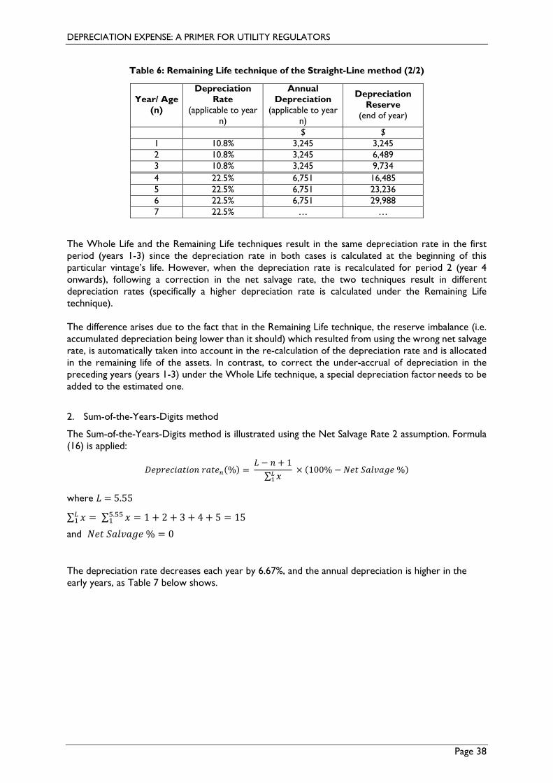
DEPRECIATION EXPENSE: A PRIMER FOR UTILITY REGULATORS
Page 38
Table 6: Remaining Life technique of the Straight-Line method (2/2)
Year/ Age (n)
Depreciation Rate
(applicable to year n)
Annual Depreciation
(applicable to year n)
Depreciation Reserve
(end of year)
$ $ 1 10.8% 3,245 3,245 2 10.8% 3,245 6,489 3 10.8% 3,245 9,734 4 22.5% 6,751 16,485 5 22.5% 6,751 23,236 6 22.5% 6,751 29,988 7 22.5% … …
The Whole Life and the Remaining Life techniques result in the same depreciation rate in the first period (years 1-3) since the depreciation rate in both cases is calculated at the beginning of this particular vintage’s life. However, when the depreciation rate is recalculated for period 2 (year 4 onwards), following a correction in the net salvage rate, the two techniques result in different depreciation rates (specifically a higher depreciation rate is calculated under the Remaining Life technique). The difference arises due to the fact that in the Remaining Life technique, the reserve imbalance (i.e. accumulated depreciation being lower than it should) which resulted from using the wrong net salvage rate, is automatically taken into account in the re-calculation of the depreciation rate and is allocated in the remaining life of the assets. In contrast, to correct the under-accrual of depreciation in the preceding years (years 1-3) under the Whole Life technique, a special depreciation factor needs to be added to the estimated one.
2. Sum-of-the-Years-Digits method
The Sum-of-the-Years-Digits method is illustrated using the Net Salvage Rate 2 assumption. Formula (16) is applied:
𝐷𝐷𝐷𝐷𝐷𝐷𝐷𝐷𝐷𝐷𝐷𝐷𝐷𝐷𝐴𝐴𝐷𝐷𝐷𝐷𝐷𝐷𝐴𝐴 𝐷𝐷𝐴𝐴𝐷𝐷𝐷𝐷𝑛𝑛(%) = 𝐿𝐿 − 𝐴𝐴 + 1∑ 𝑚𝑚𝐿𝐿1
× (100% − 𝑁𝑁𝐷𝐷𝐷𝐷 𝑆𝑆𝐴𝐴𝐴𝐴𝑆𝑆𝐴𝐴𝑆𝑆𝐷𝐷 %)
where 𝐿𝐿 = 5.55
∑ 𝑚𝑚𝐿𝐿1 = ∑ 𝑚𝑚5.551 = 1 + 2 + 3 + 4 + 5 = 15
and 𝑁𝑁𝐷𝐷𝐷𝐷 𝑆𝑆𝐴𝐴𝐴𝐴𝑆𝑆𝐴𝐴𝑆𝑆𝐷𝐷 % = 0
The depreciation rate decreases each year by 6.67%, and the annual depreciation is higher in the early years, as Table 7 below shows.
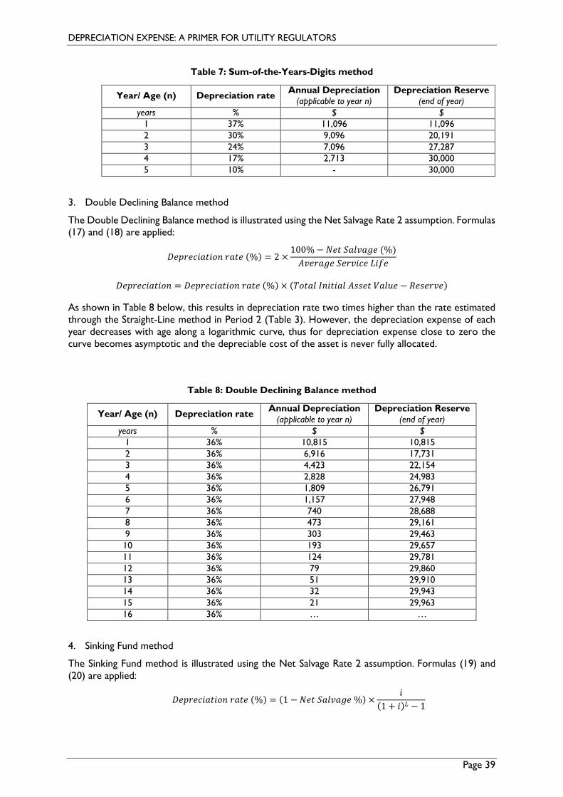
DEPRECIATION EXPENSE: A PRIMER FOR UTILITY REGULATORS
Page 39
Table 7: Sum-of-the-Years-Digits method
Year/ Age (n) Depreciation rate Annual Depreciation (applicable to year n)
Depreciation Reserve (end of year)
years % $ $ 1 37% 11,096 11,096 2 30% 9,096 20,191 3 24% 7,096 27,287 4 17% 2,713 30,000 5 10% - 30,000
3. Double Declining Balance method
The Double Declining Balance method is illustrated using the Net Salvage Rate 2 assumption. Formulas (17) and (18) are applied:
𝐷𝐷𝐷𝐷𝐷𝐷𝐷𝐷𝐷𝐷𝐷𝐷𝐷𝐷𝐴𝐴𝐷𝐷𝐷𝐷𝐷𝐷𝐴𝐴 𝐷𝐷𝐴𝐴𝐷𝐷𝐷𝐷 (%) = 2 ×100% − 𝑁𝑁𝐷𝐷𝐷𝐷 𝑆𝑆𝐴𝐴𝐴𝐴𝑆𝑆𝐴𝐴𝑆𝑆𝐷𝐷 (%)𝐴𝐴𝑆𝑆𝐷𝐷𝐷𝐷𝐴𝐴𝑆𝑆𝐷𝐷 𝑆𝑆𝐷𝐷𝐷𝐷𝑆𝑆𝐷𝐷𝐷𝐷𝐷𝐷 𝐿𝐿𝐷𝐷𝑜𝑜𝐷𝐷
𝐷𝐷𝐷𝐷𝐷𝐷𝐷𝐷𝐷𝐷𝐷𝐷𝐷𝐷𝐴𝐴𝐷𝐷𝐷𝐷𝐷𝐷𝐴𝐴 = 𝐷𝐷𝐷𝐷𝐷𝐷𝐷𝐷𝐷𝐷𝐷𝐷𝐷𝐷𝐴𝐴𝐷𝐷𝐷𝐷𝐷𝐷𝐴𝐴 𝐷𝐷𝐴𝐴𝐷𝐷𝐷𝐷 (%) × (𝑇𝑇𝐷𝐷𝐷𝐷𝐴𝐴𝐴𝐴 𝐼𝐼𝐴𝐴𝐷𝐷𝐷𝐷𝐷𝐷𝐴𝐴𝐴𝐴 𝐴𝐴𝐴𝐴𝐴𝐴𝐷𝐷𝐷𝐷 𝑉𝑉𝐴𝐴𝐴𝐴𝐴𝐴𝐷𝐷 − 𝑅𝑅𝐷𝐷𝐴𝐴𝐷𝐷𝐷𝐷𝑆𝑆𝐷𝐷)
As shown in Table 8 below, this results in depreciation rate two times higher than the rate estimated through the Straight-Line method in Period 2 (Table 3). However, the depreciation expense of each year decreases with age along a logarithmic curve, thus for depreciation expense close to zero the curve becomes asymptotic and the depreciable cost of the asset is never fully allocated.
Table 8: Double Declining Balance method
Year/ Age (n) Depreciation rate Annual Depreciation (applicable to year n)
Depreciation Reserve (end of year)
years % $ $ 1 36% 10,815 10,815 2 36% 6,916 17,731 3 36% 4,423 22,154 4 36% 2,828 24,983 5 36% 1,809 26,791 6 36% 1,157 27,948 7 36% 740 28,688 8 36% 473 29,161 9 36% 303 29,463 10 36% 193 29,657 11 36% 124 29,781 12 36% 79 29,860 13 36% 51 29,910 14 36% 32 29,943 15 36% 21 29,963 16 36% … …
4. Sinking Fund method
The Sinking Fund method is illustrated using the Net Salvage Rate 2 assumption. Formulas (19) and (20) are applied:
𝐷𝐷𝐷𝐷𝐷𝐷𝐷𝐷𝐷𝐷𝐷𝐷𝐷𝐷𝐴𝐴𝐷𝐷𝐷𝐷𝐷𝐷𝐴𝐴 𝐷𝐷𝐴𝐴𝐷𝐷𝐷𝐷 (%) = (1 − 𝑁𝑁𝐷𝐷𝐷𝐷 𝑆𝑆𝐴𝐴𝐴𝐴𝑆𝑆𝐴𝐴𝑆𝑆𝐷𝐷 %) ×𝐷𝐷
(1 + 𝐷𝐷)𝐿𝐿 − 1
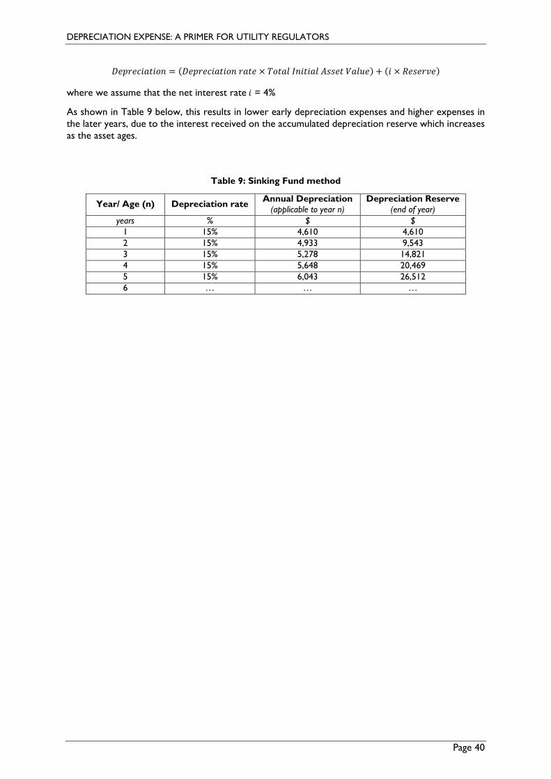
DEPRECIATION EXPENSE: A PRIMER FOR UTILITY REGULATORS
Page 40
𝐷𝐷𝐷𝐷𝐷𝐷𝐷𝐷𝐷𝐷𝐷𝐷𝐷𝐷𝐴𝐴𝐷𝐷𝐷𝐷𝐷𝐷𝐴𝐴 = (𝐷𝐷𝐷𝐷𝐷𝐷𝐷𝐷𝐷𝐷𝐷𝐷𝐷𝐷𝐴𝐴𝐷𝐷𝐷𝐷𝐷𝐷𝐴𝐴 𝐷𝐷𝐴𝐴𝐷𝐷𝐷𝐷 × 𝑇𝑇𝐷𝐷𝐷𝐷𝐴𝐴𝐴𝐴 𝐼𝐼𝐴𝐴𝐷𝐷𝐷𝐷𝐷𝐷𝐴𝐴𝐴𝐴 𝐴𝐴𝐴𝐴𝐴𝐴𝐷𝐷𝐷𝐷 𝑉𝑉𝐴𝐴𝐴𝐴𝐴𝐴𝐷𝐷) + (𝐷𝐷 × 𝑅𝑅𝐷𝐷𝐴𝐴𝐷𝐷𝐷𝐷𝑆𝑆𝐷𝐷)
where we assume that the net interest rate 𝐷𝐷 = 4%
As shown in Table 9 below, this results in lower early depreciation expenses and higher expenses in the later years, due to the interest received on the accumulated depreciation reserve which increases as the asset ages.
Table 9: Sinking Fund method
Year/ Age (n) Depreciation rate Annual Depreciation (applicable to year n)
Depreciation Reserve (end of year)
years % $ $ 1 15% 4,610 4,610 2 15% 4,933 9,543 3 15% 5,278 14,821 4 15% 5,648 20,469 5 15% 6,043 26,512 6 … … …
DEPRECIATION EXPENSE: A PRIMER FOR UTILITY REGULATORS
Page 41
Annex II: Case Studies
In this Annex, we showcase two studies on how regulators in countries with emerging economies determine allowed depreciation for electricity transmission systems, as part of the utility’s tariff-setting process. The two case studies cover Georgia and Tanzania, two countries in different regions of the world and with different age profiles of their electricity power systems.
The same organization structure is described for both case studies as follows:
• An overview of the country and its electricity sector • An overview of a utility’s allowed revenue according to the tariff regulation • The approaches followed by the regulator to define the key elements of the allowed
depreciation of regulated assets • A summary of how the concepts above are used by the regulator to estimate utility asset
depreciation. • Key findings
1. Case Study – Georgia
1.1. Country context
1.1.1. Overview of the country
Georgia is located in the Caucasus region of Eurasia and borders the Black Sea, Russia, Azerbaijan, Armenia and Turkey. It has a population of 3.7 million people. It is a developing country with an average annual economic growth of 5.3 % between 2005 and 2019.32
After Georgia’s independence in 1991, its economy went into a deep recession and major structural reforms were initiated throughout the economy.
In 2016, Georgia entered into the EU-Georgia Association Agreement and in 2017 became a Contracting party of the Energy Community Treaty. Since then, major reforms have been taking place in order to align Georgia’s energy sector with EU regulations for electricity and gas markets as well as climate and environment.
1.1.2. Overview of the Power Sector The electricity generation in Georgia is based on hydropower plants, thermal power plants and a small share of wind energy generation. The installed capacity counted 4,230 MW in 2019, consisting of 77.9% of hydro power, 21.6% of thermal power, and 0.5% of wind power capacity. Accordingly, the electricity produced in 2019, was by 75.9 % from hydropower plants, 23.4% from thermal power plants and the remaining 0.7% from wind turbines.33 The largest generation companies, Engurhesi Ltd, with an aggregate hydro plants’ installed capacity of 1,300 MW, and Vardnili Hydroplant Cascade Ltd, with hydro power capacity of 220 MW, are state owned.34 All other electricity generation companies are privately owned, and have thermal power
32 “The World Bank in Georgia.” The World Bank. https://www.worldbank.org/en/country/georgia/overview 33 “Georgian National Energy and Water Supply Regulatory Commission Report on Activities of 2019.” GNERC. https://gnerc.org/files/Annual%20Reports/Reports%20English/2019%20En.pdf 34 GNERC input
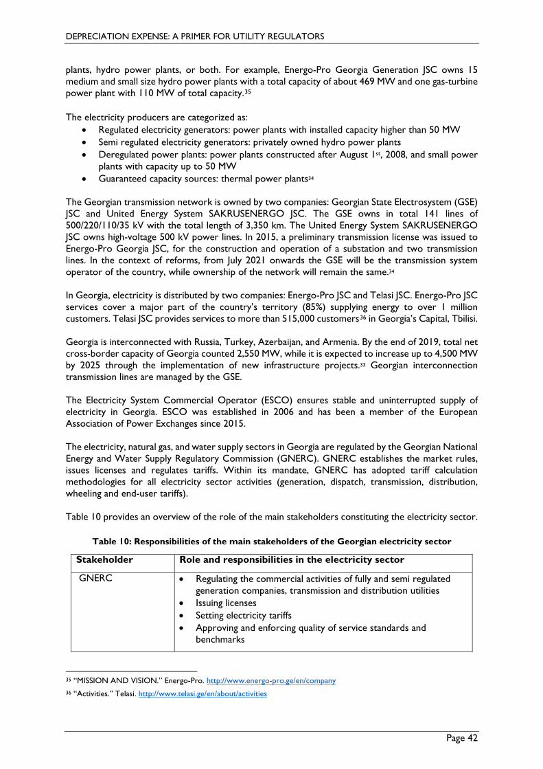
DEPRECIATION EXPENSE: A PRIMER FOR UTILITY REGULATORS
Page 42
plants, hydro power plants, or both. For example, Energo-Pro Georgia Generation JSC owns 15 medium and small size hydro power plants with a total capacity of about 469 MW and one gas-turbine power plant with 110 MW of total capacity.35 The electricity producers are categorized as:
• Regulated electricity generators: power plants with installed capacity higher than 50 MW • Semi regulated electricity generators: privately owned hydro power plants • Deregulated power plants: power plants constructed after August 1st, 2008, and small power
plants with capacity up to 50 MW • Guaranteed capacity sources: thermal power plants34
The Georgian transmission network is owned by two companies: Georgian State Electrosystem (GSE) JSC and United Energy System SAKRUSENERGO JSC. The GSE owns in total 141 lines of 500/220/110/35 kV with the total length of 3,350 km. The United Energy System SAKRUSENERGO JSC owns high-voltage 500 kV power lines. In 2015, a preliminary transmission license was issued to Energo-Pro Georgia JSC, for the construction and operation of a substation and two transmission lines. In the context of reforms, from July 2021 onwards the GSE will be the transmission system operator of the country, while ownership of the network will remain the same.34 In Georgia, electricity is distributed by two companies: Energo-Pro JSC and Telasi JSC. Energo-Pro JSC services cover a major part of the country’s territory (85%) supplying energy to over 1 million customers. Telasi JSC provides services to more than 515,000 customers36 in Georgia’s Capital, Tbilisi. Georgia is interconnected with Russia, Turkey, Azerbaijan, and Armenia. By the end of 2019, total net cross-border capacity of Georgia counted 2,550 MW, while it is expected to increase up to 4,500 MW by 2025 through the implementation of new infrastructure projects.33 Georgian interconnection transmission lines are managed by the GSE. The Electricity System Commercial Operator (ESCO) ensures stable and uninterrupted supply of electricity in Georgia. ESCO was established in 2006 and has been a member of the European Association of Power Exchanges since 2015. The electricity, natural gas, and water supply sectors in Georgia are regulated by the Georgian National Energy and Water Supply Regulatory Commission (GNERC). GNERC establishes the market rules, issues licenses and regulates tariffs. Within its mandate, GNERC has adopted tariff calculation methodologies for all electricity sector activities (generation, dispatch, transmission, distribution, wheeling and end-user tariffs). Table 10 provides an overview of the role of the main stakeholders constituting the electricity sector.
Table 10: Responsibilities of the main stakeholders of the Georgian electricity sector
Stakeholder Role and responsibilities in the electricity sector
GNERC • Regulating the commercial activities of fully and semi regulated generation companies, transmission and distribution utilities
• Issuing licenses • Setting electricity tariffs • Approving and enforcing quality of service standards and
benchmarks
35 “MISSION AND VISION.” Energo-Pro. http://www.energo-pro.ge/en/company 36 “Activities.” Telasi. http://www.telasi.ge/en/about/activities
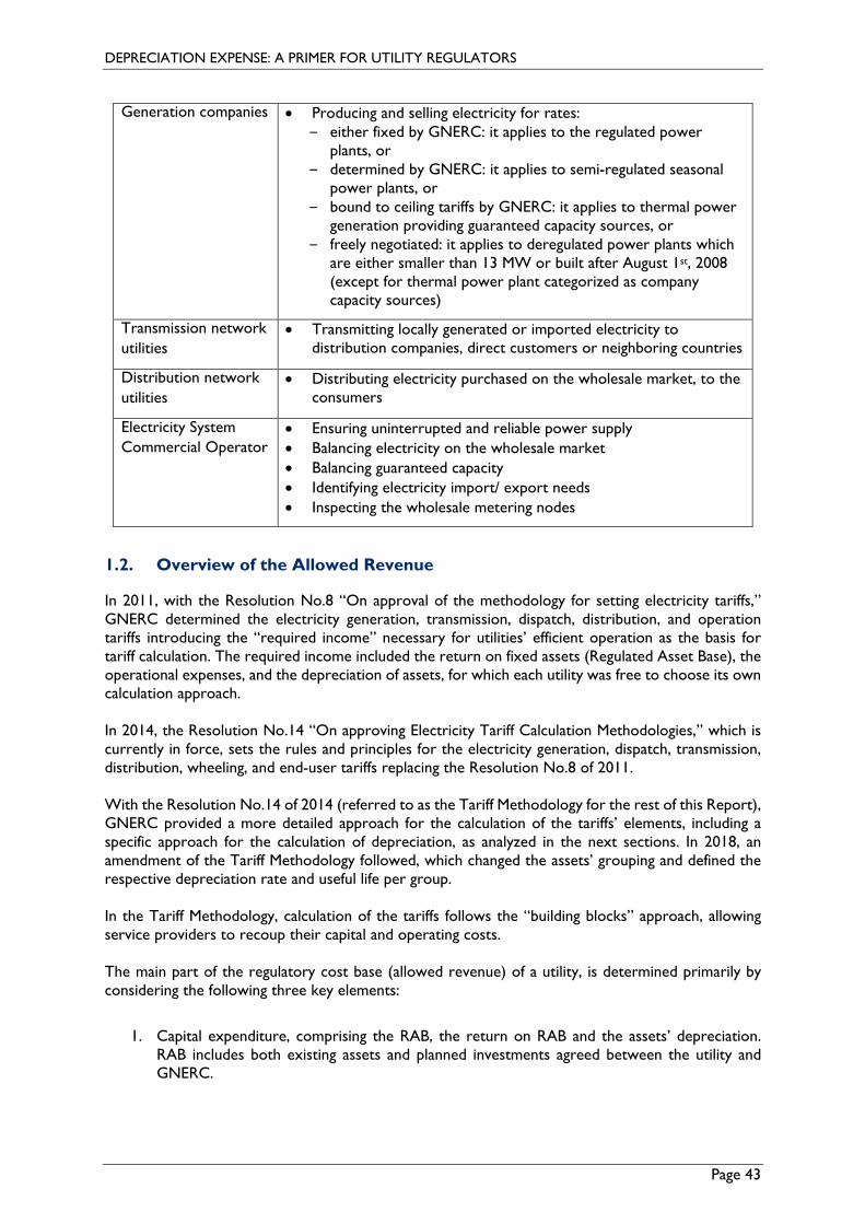
DEPRECIATION EXPENSE: A PRIMER FOR UTILITY REGULATORS
Page 43
Generation companies • Producing and selling electricity for rates: ‒ either fixed by GNERC: it applies to the regulated power
plants, or ‒ determined by GNERC: it applies to semi-regulated seasonal
power plants, or ‒ bound to ceiling tariffs by GNERC: it applies to thermal power
generation providing guaranteed capacity sources, or ‒ freely negotiated: it applies to deregulated power plants which
are either smaller than 13 MW or built after August 1st, 2008 (except for thermal power plant categorized as company capacity sources)
Transmission network utilities
• Transmitting locally generated or imported electricity to distribution companies, direct customers or neighboring countries
Distribution network utilities
• Distributing electricity purchased on the wholesale market, to the consumers
Electricity System Commercial Operator
• Ensuring uninterrupted and reliable power supply • Balancing electricity on the wholesale market • Balancing guaranteed capacity • Identifying electricity import/ export needs • Inspecting the wholesale metering nodes
1.2. Overview of the Allowed Revenue
In 2011, with the Resolution No.8 “On approval of the methodology for setting electricity tariffs,” GNERC determined the electricity generation, transmission, dispatch, distribution, and operation tariffs introducing the “required income” necessary for utilities’ efficient operation as the basis for tariff calculation. The required income included the return on fixed assets (Regulated Asset Base), the operational expenses, and the depreciation of assets, for which each utility was free to choose its own calculation approach. In 2014, the Resolution No.14 “On approving Electricity Tariff Calculation Methodologies,” which is currently in force, sets the rules and principles for the electricity generation, dispatch, transmission, distribution, wheeling, and end-user tariffs replacing the Resolution No.8 of 2011. With the Resolution No.14 of 2014 (referred to as the Tariff Methodology for the rest of this Report), GNERC provided a more detailed approach for the calculation of the tariffs’ elements, including a specific approach for the calculation of depreciation, as analyzed in the next sections. In 2018, an amendment of the Tariff Methodology followed, which changed the assets’ grouping and defined the respective depreciation rate and useful life per group. In the Tariff Methodology, calculation of the tariffs follows the “building blocks” approach, allowing service providers to recoup their capital and operating costs. The main part of the regulatory cost base (allowed revenue) of a utility, is determined primarily by considering the following three key elements:
1. Capital expenditure, comprising the RAB, the return on RAB and the assets’ depreciation. RAB includes both existing assets and planned investments agreed between the utility and GNERC.
DEPRECIATION EXPENSE: A PRIMER FOR UTILITY REGULATORS
Page 44
2. Controllable and uncontrollable operating expenses, with controllable expenses being adjusted annually by an inflation indicator CPI and an efficiency factor X.
3. Costs for filling normative losses in the electricity network. These are defined on the basis of a weighted average purchase price (estimated according to the planned electricity purchases by the utility in the regulatory period to compensate for losses), and the amount of electricity normative losses (calculated according to GNERC Resolution No.15 of 2014 by using inter-alia actual data for the base year and the trend of the actual losses of three previous years).
Other elements (i.e. the interest cost of working capital and service quality components) are also included in the calculation of a utility’s allowed revenue. A year-on-year correction mechanism to cover over/under-recovery of tariffs is also foreseen. The focus of this case study is on the treatment of the depreciation of assets by GNERC.
1.3. Main dimensions and inputs of the Depreciation System
In this section we provide a description of the approaches followed by GNERC to define the key elements of the allowed depreciation of regulated assets, applied for electricity transmission tariffs.
1.3.1. Initial Value of Assets According to GNERC’s Tariff Methodology, for the calculation of allowed depreciation, a utility should determine the initial value of its assets based on a “historic costs” approach. The Georgian electricity network infrastructure comprises new assets, constructed after 2000, as well as old assets, dating back to the period when Georgia was part of the Soviet Union. After 1995 and mainly in the 2000s and 2010s, when several investments were made in the Georgian power sector, utilities kept records of their investments. However, regarding the older assets before the beginning of energy sector reforms in 1995, there was no regulatory set up requiring any property records, resulting in unavailability of old assets’ cost data. To address the issue of missing cost data for old assets, GNERC provides in the Tariff Methodology that in cases where cost records are not available, “replacement costs” shall be used as a one – time proxy. If, for instance, a utility owns an asset that was constructed back in the 1990s, and there is no record of the original cost of acquiring this asset, while the costs of additional investments that were made on the asset in 2007 and subsequent years, have been recorded, the utility should determine the 2007 replacement costs of developing a new asset of the same type and depreciate/ adjust these costs to reflect the condition of the existing asset. The resulting value constitutes the initial value of the asset determined by following the replacement costs approach. All the subsequent costs, because of the additions in 2007 onwards, should be treated as historic costs, and added to the asset’s initial value.
1.3.2. Revaluation of Assets As far as the assets’ revaluation is concerned, there is no provision about this in the current Tariff Methodology. The value of assets is fixed since their first valuation, and no periodic re-adjustment due to potential variations in the inflation and/ or currency risk, is foreseen. However, Georgian utilities, which often take loans in foreign currency (dollars/ euros) while making investments in the local
DEPRECIATION EXPENSE: A PRIMER FOR UTILITY REGULATORS
Page 45
currency (Georgian Lari (GEL)), have requested from GNERC a framework for their assets’ revaluation, since they are directly affected by any change in the currency exchange rates.
1.3.3. Impairment tests for statutory accounts Utilities are obliged to carry out their accounting and financial recording based on the Unified System of Accounting. 2020 was the first year these guidelines were implemented. Regarding the statutory accounts of the utilities, the Tariff Methodology includes provisions on how impairment test results are to be used, without clearly setting an obligation to the utilities for executing such tests for the statutory accounts. There are also provisions that protect utilities from unexpected/ uncontrollable circumstances. For example, in case of major legal changes causing steep decrease in the value of a utility’s assets, the impairment test results are not taken into account, and thus the allowed return on those assets are calculated as before.
1.3.4. Salvage Value of Assets The mechanism applied by GNERC for estimating the salvage value of assets, and for treating the sale of assets, incentivizes utilities to use their assets until the end of their useful life, i.e., until their value is fully depreciated. The tariff methodology stipulates that:
• If the utility retires an asset upon the end of its useful life, the net salvage value of the asset at its retirement equals to zero. In case the utility sells this retired, completely depreciated, regulated asset, then 50% of the profit received from the sale is deducted from the utility’s allowed revenue.
• On the other hand, if the utility sells an asset before it is completely depreciated, then 100% of the profit made from the sale of this ‘incompletely used-up’ regulated asset, is subtracted from the allowed revenue. In this case, the asset’s salvage value is equal to the asset’s net book value in the year of its retirement.
1.3.5. Grouping of Assets GNERC groups together units of the same type and similar characteristics, which are used in the same way and operate under the same conditions (“broad groups”). The grouping Procedure is carried out by the technical department of GNERC. At this level of “broad groups” the life characteristics of the assets (i.e., service life and depreciation rate) are determined. Examples of broad groups include:
• Overhead lines of 110kV and above • Overhead lines of 35kV • Overhead lines 6/10 kV • Overhead lines 220/380 V • Power transformers • Distribution equipment (bus bar) • Overvoltage protection equipment • Converters (rectifiers, inverters, and voltage regulators)
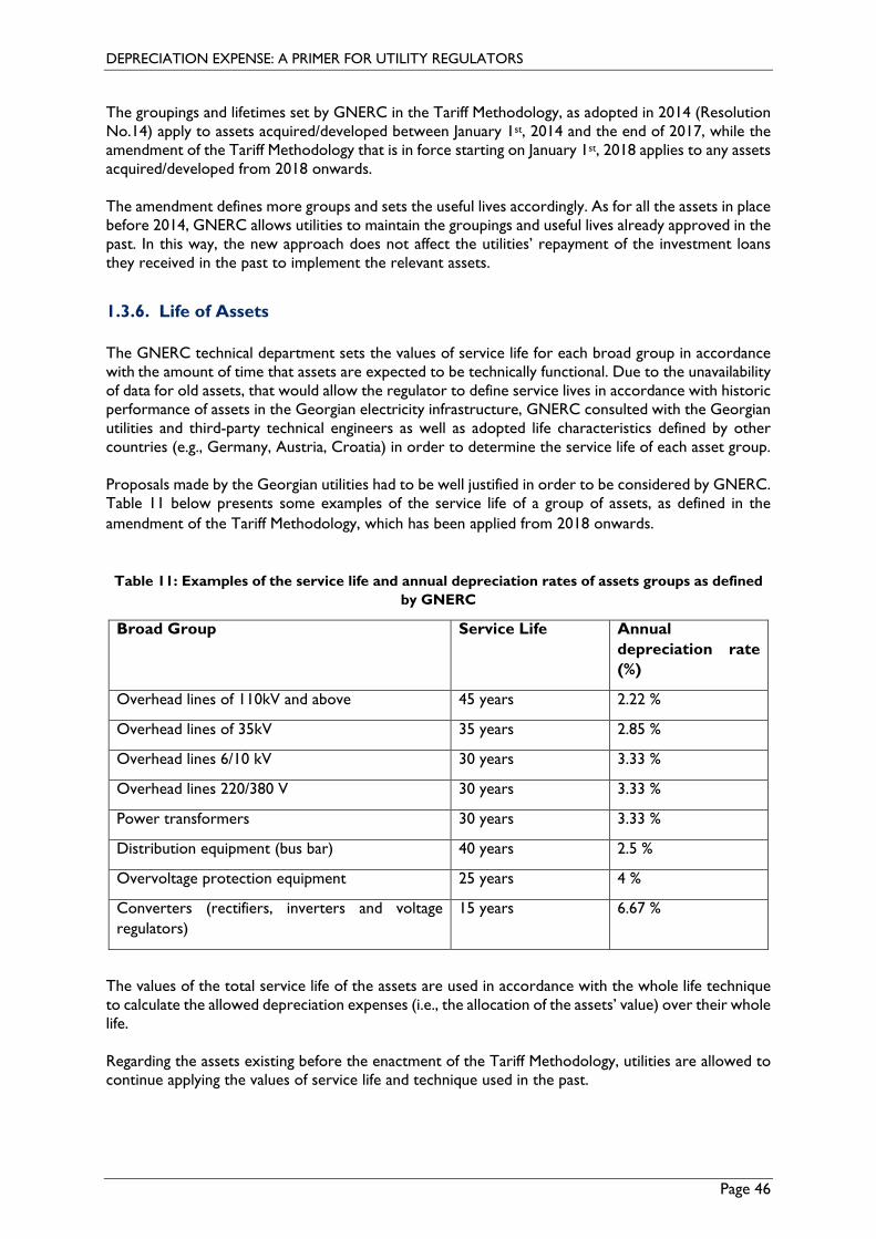
DEPRECIATION EXPENSE: A PRIMER FOR UTILITY REGULATORS
Page 46
The groupings and lifetimes set by GNERC in the Tariff Methodology, as adopted in 2014 (Resolution No.14) apply to assets acquired/developed between January 1st, 2014 and the end of 2017, while the amendment of the Tariff Methodology that is in force starting on January 1st, 2018 applies to any assets acquired/developed from 2018 onwards. The amendment defines more groups and sets the useful lives accordingly. As for all the assets in place before 2014, GNERC allows utilities to maintain the groupings and useful lives already approved in the past. In this way, the new approach does not affect the utilities’ repayment of the investment loans they received in the past to implement the relevant assets.
1.3.6. Life of Assets The GNERC technical department sets the values of service life for each broad group in accordance with the amount of time that assets are expected to be technically functional. Due to the unavailability of data for old assets, that would allow the regulator to define service lives in accordance with historic performance of assets in the Georgian electricity infrastructure, GNERC consulted with the Georgian utilities and third-party technical engineers as well as adopted life characteristics defined by other countries (e.g., Germany, Austria, Croatia) in order to determine the service life of each asset group. Proposals made by the Georgian utilities had to be well justified in order to be considered by GNERC. Table 11 below presents some examples of the service life of a group of assets, as defined in the amendment of the Tariff Methodology, which has been applied from 2018 onwards.
Table 11: Examples of the service life and annual depreciation rates of assets groups as defined by GNERC
Broad Group Service Life Annual depreciation rate (%)
Overhead lines of 110kV and above 45 years 2.22 %
Overhead lines of 35kV 35 years 2.85 %
Overhead lines 6/10 kV 30 years 3.33 %
Overhead lines 220/380 V 30 years 3.33 %
Power transformers 30 years 3.33 %
Distribution equipment (bus bar) 40 years 2.5 %
Overvoltage protection equipment 25 years 4 %
Converters (rectifiers, inverters and voltage regulators)
15 years 6.67 %
The values of the total service life of the assets are used in accordance with the whole life technique to calculate the allowed depreciation expenses (i.e., the allocation of the assets’ value) over their whole life. Regarding the assets existing before the enactment of the Tariff Methodology, utilities are allowed to continue applying the values of service life and technique used in the past.
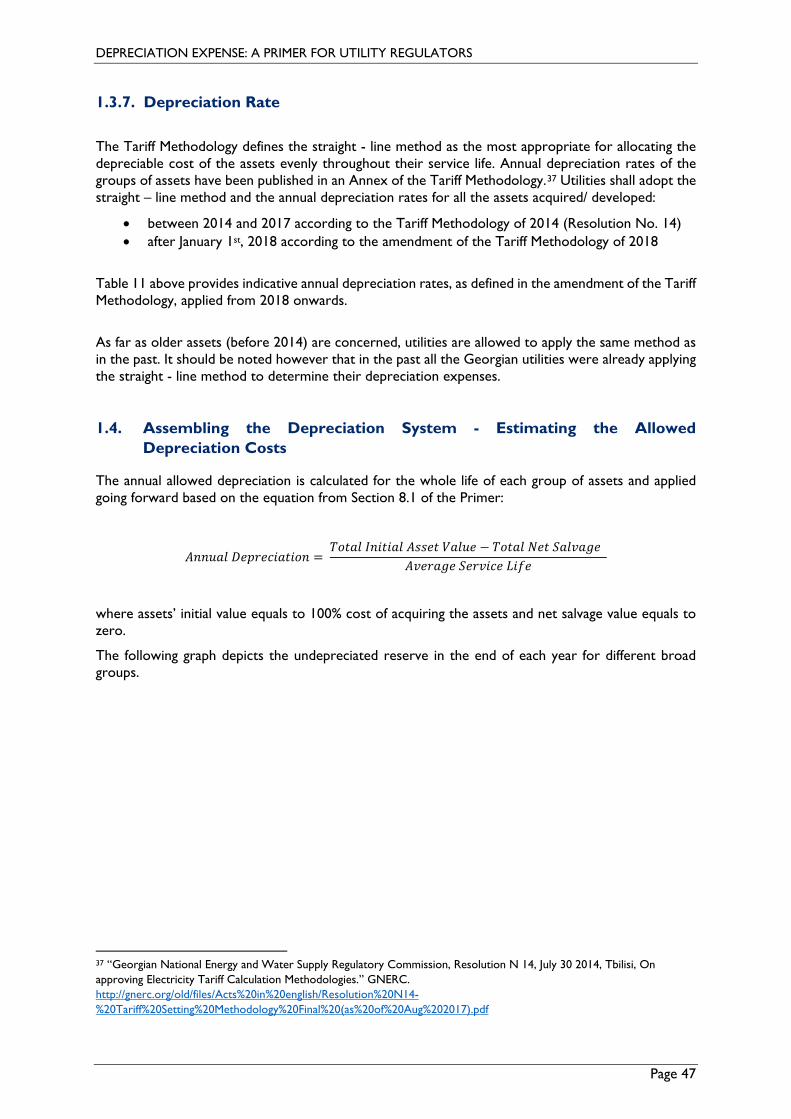
DEPRECIATION EXPENSE: A PRIMER FOR UTILITY REGULATORS
Page 47
1.3.7. Depreciation Rate
The Tariff Methodology defines the straight - line method as the most appropriate for allocating the depreciable cost of the assets evenly throughout their service life. Annual depreciation rates of the groups of assets have been published in an Annex of the Tariff Methodology.37 Utilities shall adopt the straight – line method and the annual depreciation rates for all the assets acquired/ developed:
• between 2014 and 2017 according to the Tariff Methodology of 2014 (Resolution No. 14) • after January 1st, 2018 according to the amendment of the Tariff Methodology of 2018
Table 11 above provides indicative annual depreciation rates, as defined in the amendment of the Tariff Methodology, applied from 2018 onwards.
As far as older assets (before 2014) are concerned, utilities are allowed to apply the same method as in the past. It should be noted however that in the past all the Georgian utilities were already applying the straight - line method to determine their depreciation expenses.
1.4. Assembling the Depreciation System - Estimating the Allowed Depreciation Costs
The annual allowed depreciation is calculated for the whole life of each group of assets and applied going forward based on the equation from Section 8.1 of the Primer:
𝐴𝐴𝐴𝐴𝐴𝐴𝐴𝐴𝐴𝐴𝐴𝐴 𝐷𝐷𝐷𝐷𝐷𝐷𝐷𝐷𝐷𝐷𝐷𝐷𝐷𝐷𝐴𝐴𝐷𝐷𝐷𝐷𝐷𝐷𝐴𝐴 = 𝑇𝑇𝐷𝐷𝐷𝐷𝐴𝐴𝐴𝐴 𝐼𝐼𝐴𝐴𝐷𝐷𝐷𝐷𝐷𝐷𝐴𝐴𝐴𝐴 𝐴𝐴𝐴𝐴𝐴𝐴𝐷𝐷𝐷𝐷 𝑉𝑉𝐴𝐴𝐴𝐴𝐴𝐴𝐷𝐷 − 𝑇𝑇𝐷𝐷𝐷𝐷𝐴𝐴𝐴𝐴 𝑁𝑁𝐷𝐷𝐷𝐷 𝑆𝑆𝐴𝐴𝐴𝐴𝑆𝑆𝐴𝐴𝑆𝑆𝐷𝐷
𝐴𝐴𝑆𝑆𝐷𝐷𝐷𝐷𝐴𝐴𝑆𝑆𝐷𝐷 𝑆𝑆𝐷𝐷𝐷𝐷𝑆𝑆𝐷𝐷𝐷𝐷𝐷𝐷 𝐿𝐿𝐷𝐷𝑜𝑜𝐷𝐷
where assets’ initial value equals to 100% cost of acquiring the assets and net salvage value equals to zero.
The following graph depicts the undepreciated reserve in the end of each year for different broad groups.
37 “Georgian National Energy and Water Supply Regulatory Commission, Resolution N 14, July 30 2014, Tbilisi, On approving Electricity Tariff Calculation Methodologies.” GNERC. http://gnerc.org/old/files/Acts%20in%20english/Resolution%20N14-%20Tariff%20Setting%20Methodology%20Final%20(as%20of%20Aug%202017).pdf
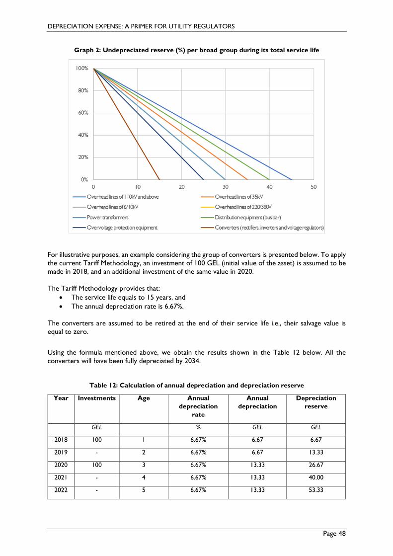
DEPRECIATION EXPENSE: A PRIMER FOR UTILITY REGULATORS
Page 48
Graph 2: Undepreciated reserve (%) per broad group during its total service life
For illustrative purposes, an example considering the group of converters is presented below. To apply the current Tariff Methodology, an investment of 100 GEL (initial value of the asset) is assumed to be made in 2018, and an additional investment of the same value in 2020. The Tariff Methodology provides that:
• The service life equals to 15 years, and • The annual depreciation rate is 6.67%.
The converters are assumed to be retired at the end of their service life i.e., their salvage value is equal to zero.
Using the formula mentioned above, we obtain the results shown in the Table 12 below. All the converters will have been fully depreciated by 2034.
Table 12: Calculation of annual depreciation and depreciation reserve
Year Investments Age Annual depreciation
rate
Annual depreciation
Depreciation reserve
GEL % GEL GEL
2018 100 1 6.67% 6.67 6.67
2019 - 2 6.67% 6.67 13.33
2020 100 3 6.67% 13.33 26.67
2021 - 4 6.67% 13.33 40.00
2022 - 5 6.67% 13.33 53.33
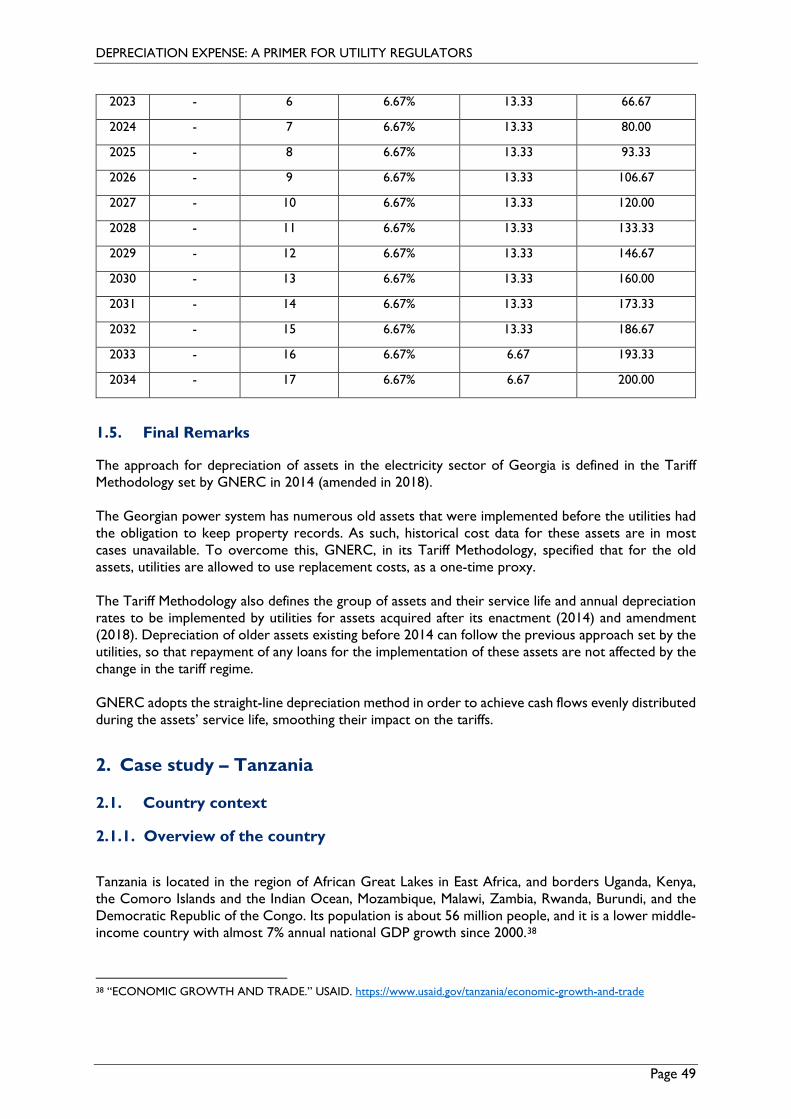
DEPRECIATION EXPENSE: A PRIMER FOR UTILITY REGULATORS
Page 49
2023 - 6 6.67% 13.33 66.67
2024 - 7 6.67% 13.33 80.00
2025 - 8 6.67% 13.33 93.33
2026 - 9 6.67% 13.33 106.67
2027 - 10 6.67% 13.33 120.00
2028 - 11 6.67% 13.33 133.33
2029 - 12 6.67% 13.33 146.67
2030 - 13 6.67% 13.33 160.00
2031 - 14 6.67% 13.33 173.33
2032 - 15 6.67% 13.33 186.67
2033 - 16 6.67% 6.67 193.33
2034 - 17 6.67% 6.67 200.00
1.5. Final Remarks
The approach for depreciation of assets in the electricity sector of Georgia is defined in the Tariff Methodology set by GNERC in 2014 (amended in 2018). The Georgian power system has numerous old assets that were implemented before the utilities had the obligation to keep property records. As such, historical cost data for these assets are in most cases unavailable. To overcome this, GNERC, in its Tariff Methodology, specified that for the old assets, utilities are allowed to use replacement costs, as a one-time proxy. The Tariff Methodology also defines the group of assets and their service life and annual depreciation rates to be implemented by utilities for assets acquired after its enactment (2014) and amendment (2018). Depreciation of older assets existing before 2014 can follow the previous approach set by the utilities, so that repayment of any loans for the implementation of these assets are not affected by the change in the tariff regime. GNERC adopts the straight-line depreciation method in order to achieve cash flows evenly distributed during the assets’ service life, smoothing their impact on the tariffs.
2. Case study – Tanzania
2.1. Country context
2.1.1. Overview of the country
Tanzania is located in the region of African Great Lakes in East Africa, and borders Uganda, Kenya, the Comoro Islands and the Indian Ocean, Mozambique, Malawi, Zambia, Rwanda, Burundi, and the Democratic Republic of the Congo. Its population is about 56 million people, and it is a lower middle-income country with almost 7% annual national GDP growth since 2000.38
38 “ECONOMIC GROWTH AND TRADE.” USAID. https://www.usaid.gov/tanzania/economic-growth-and-trade
DEPRECIATION EXPENSE: A PRIMER FOR UTILITY REGULATORS
Page 50
In 2020, the country achieved the highest percentage in access to electricity so far (84.6%)39. To reach this level of development, the country has undergone several energy-sector reforms aiming to attract private investments, increase electricity supply and meet demand. An important part of the reforms is the effort for regulating electricity and adopting cost-reflective tariffs.
2.1.2. Overview of the Power Sector
As of June 30th, 2019, the installed capacity was 1,600 MW of which 1,560 MW was connected to the main grid and 37 MW were off grids. This capacity does not take into account industries with own use generation capacity of about 197 MW. The generation mix consisted of natural gas 67.5%, hydropower 32.3%, liquid fuel (HFO/IDO/GO) 0.1%, and biomass 0.2%. The electricity generation counted around 7.5 TWh.40 Tanzania Electric Supply Company Limited (TANESCO), which is a public and vertically integrated utility, dominates the electricity sector. It is engaged in electricity generation, transmission, distribution, supply and cross border trade activities.
Private utilities have a relatively small role in the electricity sector. Indicatively, Mwenga Hydropower Limited (MHL) and Andoya Hydro Electric Power Company Limited (AHEPO) are active in electricity generation and distribution activities. The transmission network comprises 5,896 km, of which 543 km are 66 kV lines, 1,673 km of 132 kV lines, 3,011 km of 220 kV lines, and 670 km of 400 kV lines. The distribution network comprises of approximately 109,663 km, of which 109,225 km are owned and operated by TANESCO, 414 km by Mwenga Power Services Limited, and 24 km by Andoya Hydro Electric Power Company Limited.40 The Energy and Water Utilities Regulatory Authority (EWURA) started its operation in 2006, and is responsible for the technical and economic regulation of the electricity sector in Tanzania. All utilities pursuing electricity generation, transmission, distribution, supply, system operation, and cross-border trade with respect to capacity higher than 1 MW, should hold the respective license issued by EWURA. For utilities providing services below 1 MW capacity, licensing is not required, but their registration at EWURA is obligatory. EWURA approves and enforces tariffs and fees charged by utilities and ensures quality and reliability of electricity supply. Table 13 provides an overview of the responsibilities of the main stakeholders in the Tanzanian electricity sector.
39 “Tanzania records highest percentage in access to electricity.” ESI Africa. https://www.esi-africa.com/industry-sectors/transmission-and-distribution/tanzania-records-highest-percentage-in-access-to-electricity/ 40 “THE ELECTRICITY SUB – SECTOR REGULATORY PERFORMANCE REPORT FOR THE FINANCIAL YEAR 2018/2019.” EWURA, https://www.ewura.go.tz/wp-content/uploads/2020/07/Regulatory-Performance-Report-on-Electricity-Sub-sector-for-the-Year-2019.pdf
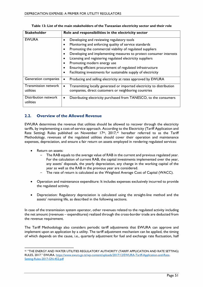
DEPRECIATION EXPENSE: A PRIMER FOR UTILITY REGULATORS
Page 51
Table 13: List of the main stakeholders of the Tanzanian electricity sector and their role
Stakeholder Role and responsibilities in the electricity sector
EWURA • Developing and reviewing regulatory tools • Monitoring and enforcing quality of service standards • Promoting the commercial viability of regulated suppliers • Developing and implementing measures to protect consumer interests • Licensing and registering regulated electricity suppliers • Promoting modern energy use • Ensuring efficient procurement of regulated infrastructure • Facilitating investments for sustainable supply of electricity
Generation companies • Producing and selling electricity at rates approved by EWURA
Transmission network utilities
• Transmitting locally generated or imported electricity to distribution companies, direct customers or neighboring countries
Distribution network utilities
• Distributing electricity purchased from TANESCO, to the consumers
2.2. Overview of the Allowed Revenue
EWURA determines the revenue that utilities should be allowed to recover through the electricity tariffs, by implementing a cost-of-service approach. According to the Electricity (Tariff Application and Rate Setting) Rules published on November 17th, 2017,41 hereafter referred to as the Tariff Methodology, revenues of the regulated utilities should cover their operation and maintenance expenses, depreciation, and ensure a fair return on assets employed in rendering regulated services:
• Return on assets: ‒ The RAB equals to the average value of RAB in the current and previous regulated year.
For the calculation of current RAB, the capital investments implemented over the year, any assets’ disposals, the yearly depreciation, any change in the working capital of the year as well as the RAB in the previous year are considered.
‒ The rate of return is calculated as the Weighted Average Cost of Capital (WACC).
• Operation and maintenance expenditure: It includes expenses exclusively incurred to provide the regulated activity.
• Depreciation: Regulatory depreciation is calculated using the straight-line method and the assets’ remaining life, as described in the following sections.
In case of the transmission system operator, other revenues related to the regulated activity including the net amount (revenues – expenditures) realized through the cross-border trade are deducted from the revenue requirement. The Tariff Methodology also considers periodic tariff adjustments that EWURA can approve and implement upon an application by a utility. The tariff adjustment mechanism can be applied, the timing of which depends on the cause, i.e., quarterly adjustment for fuel and exchange rate fluctuation, half
41 “THE ENERGY AND WATER UTILITIES REGULATORY AUTHORITY (TARIFF APPLICATION AND RATE SETTING) RULES, 2017.” EWURA. https://www.ewura.go.tz/wp-content/uploads/2017/12/EWURA-Tariff-Application-and-Rate-Setting-Rules-2017-GN-452.pdf
DEPRECIATION EXPENSE: A PRIMER FOR UTILITY REGULATORS
Page 52
yearly for inflation, and annually planned projects implementation. Tariff adjustments can also be made in cases where a utility receives a tax exemption, grant or subsidy from the Government.
The focus of this case study is on the treatment of the depreciation of assets by EWURA.
2.3. Main dimensions and inputs of the Depreciation System
In this section, we provide a description of the approaches followed by EWURA to define the key elements of the allowed depreciation of regulated assets, applied for electricity transmission tariffs.
2.3.1. Initial Value of Assets According to EWURA’s Tariff Methodology, for the calculation of allowed depreciation, a utility should determine the initial value of its assets based on a “historic costs” approach. This approach requires purchasing costs to be recorded.
In practice, historic costs, reflecting actual costs, are used in most cases for determining the initial value of the assets. Nevertheless, EWURA has considered cases that accounting data are not available; in such cases, either the cost of replacing current assets with new assets (replacement cost), or benchmarking, taking into account data by utilities of neighboring countries, can be used for estimating assets’ initial value. Indicatively, the replacement cost approach was applied during the 2012/13 tariff review.
2.3.2. Revaluation of Assets As far as the revaluation of assets is concerned, according to Tariff Application Guidelines for Regulated Utilities in Electricity and Natural Gas Subsectors,42 International Financial Reporting Standards (IFRS) and International Valuation Standards (IVS) requirements should be followed. The assets’ revaluation is determined in accordance with the utility’s policy. TANESCO states in its annual reports that the utility’s management team is responsible for identifying the need for assets’ revaluation, while the periodic assets’ revaluations are carried out by external independent experts/ valuers. In the period 2015 – 2016, a revaluation took place. In this revaluation, transmission assets were valued by following the net replacement cost approach, i.e., the new values of the assets were determined by the current replacement costs of developing/ acquiring new assets with similar characteristics (e.g., voltage level) and depreciated according to the age, economic obsolescence, and condition of the existing assets.
2.3.3. Impairment tests for statutory accounts
Regulated utilities are obliged to carry out their accounting and financial recording following the International Financial Reporting Standards (IFRS).
42 “Tariff Application Guidelines for Regulated Utilities in the Electricity and Natural Gas Subsectors.” EWURA. https://www.ewura.go.tz/wp-content/uploads/2015/04/Tariff-Application-Guidelines-for-Electricity-and-Natural-Gas-2017.pdf
DEPRECIATION EXPENSE: A PRIMER FOR UTILITY REGULATORS
Page 53
Regarding the statutory accounts of the utilities, the utilities are obliged to carry out impairment tests. According to TANESCO’s annual reports, the utility’s directors are responsible for estimating the carrying amount/ book value of impaired assets. Impairment tests are executed when there are events/ changes indicating that assets’ book value may not be recovered.
2.3.4. Salvage Value of Assets Transmission utilities determine the salvage value of the assets at the end of their useful life, taking into account the discounted free cash flow of the last year. Any removal costs are subtracted in order to estimate the net salvage value of the assets. According to TANESCO’s annual reports, salvage values are reviewed periodically, and appropriate adjustments are made. In the Tanzanian transmission grid, retirements of assets have not occurred so far. This applies even in cases of aged assets, because of the frequent replacements of the aged assets’ parts that ensure continuing reliable provision of services.
2.3.5. Grouping of Assets EWURA follows the broad group approach and defines the following three group of transmission assets:
1. Substations of 400kVA, 220kVA, 66kVA capacities, 2. SCADA – control centers, and 3. High Voltage Transmission Lines of 66kV, 132kV, 220kV and 400kV voltage levels.
2.3.6. Life of Assets EWURA sets the values of service life for each broad group by adopting benchmarking of transmission assets of similar utilities. The maximum service life of 50 years is assigned to High Voltage Transmission Lines group, while an average 35-year service life is considered a representative economic life of the transmission assets of all three groups. The Tariff Methodology considers the remaining useful economic life of each asset in the calculation of allowed depreciation.
2.3.7. Depreciation Rate The Tariff Methodology defines the straight - line method as the most appropriate for allocating the regulatory asset base throughout the remaining service life of the assets. The depreciation rate is determined by dividing the annual depreciation by the initial value of the assets. The Tariff Methodology provides the equation for calculating annual depreciation, as presented in the following section 3.4.
DEPRECIATION EXPENSE: A PRIMER FOR UTILITY REGULATORS
Page 54
2.4. Assembling the Depreciation System - Estimating the Allowed Depreciation Costs
The Tariff Methodology defines the following equation for calculating annual regulatory depreciation for each asset:
𝐴𝐴𝐴𝐴𝐴𝐴𝐴𝐴𝐴𝐴𝐴𝐴 𝐷𝐷𝐷𝐷𝐷𝐷𝐷𝐷𝐷𝐷𝐷𝐷𝐷𝐷𝐴𝐴𝐷𝐷𝐷𝐷𝐷𝐷𝐴𝐴 𝐷𝐷𝑜𝑜 𝐷𝐷𝐴𝐴𝐷𝐷ℎ 𝐴𝐴𝐴𝐴𝐴𝐴𝐷𝐷𝐷𝐷 = 𝑅𝑅𝐴𝐴𝐵𝐵 of each asset
𝐴𝐴𝑆𝑆𝐷𝐷𝐷𝐷𝐴𝐴𝑆𝑆𝐷𝐷 𝑅𝑅𝐷𝐷𝑅𝑅𝐴𝐴𝐷𝐷𝐴𝐴𝐷𝐷𝐴𝐴𝑆𝑆 𝑆𝑆𝐷𝐷𝐷𝐷𝑆𝑆𝐷𝐷𝐷𝐷𝐷𝐷 𝐿𝐿𝐷𝐷𝑜𝑜𝐷𝐷 𝐷𝐷𝑜𝑜 𝐷𝐷𝐴𝐴𝐷𝐷ℎ 𝐴𝐴𝐴𝐴𝐴𝐴𝐷𝐷𝐷𝐷
where:
RAB of each asset in the current year t is:
𝑅𝑅𝐴𝐴𝐵𝐵𝑡𝑡 = 𝑅𝑅𝐴𝐴𝐵𝐵𝑡𝑡−1 + 𝐼𝐼𝐴𝐴𝑆𝑆𝐷𝐷𝐴𝐴𝐷𝐷𝑅𝑅𝐷𝐷𝐴𝐴𝐷𝐷 𝐴𝐴𝑢𝑢𝑢𝑢𝐷𝐷𝐷𝐷𝐷𝐷𝐷𝐷𝐴𝐴𝐴𝐴𝑡𝑡 − 𝐷𝐷𝐷𝐷𝐴𝐴𝐷𝐷𝐷𝐷𝐴𝐴𝐴𝐴𝐴𝐴𝐴𝐴𝑡𝑡 − 𝐷𝐷𝐷𝐷𝐷𝐷𝐷𝐷𝐷𝐷𝐷𝐷𝐷𝐷𝐴𝐴𝐷𝐷𝐷𝐷𝐷𝐷𝐴𝐴𝑡𝑡 + 𝛥𝛥(𝑅𝑅𝐷𝐷𝐷𝐷𝑊𝑊𝐷𝐷𝐴𝐴𝑆𝑆 𝐶𝐶𝐴𝐴𝐷𝐷𝐷𝐷𝐷𝐷𝐴𝐴𝐴𝐴)𝑡𝑡.
This approach of calculating annual depreciation appears to provide the regulator with the flexibility to adjust accordingly the regulatory depreciation, reflecting extraordinary changes on the RAB’s value, mitigating inflationary and currency risk, as well as impairment tests results, limiting the likelihood of sharp tariff increases.
2.5. Final Remarks
The approach for depreciation of assets in the electricity transmission sector of Tanzania is defined in the Tariff Methodology set by EWURA in 2017. In Tanzania, in most cases the utilities keep property records. As such, historic cost data are used for determining the initial value of the assets. In case of unavailability of historic data, EWURA defines the replacement cost approach, or benchmarking, taking into account data by utilities of neighboring countries, for calculating the initial value of the assets. EWURA also defines three broad groups for the transmission assets and their service life. The calculation of depreciation is based on the straight-line method and the remaining useful life of assets, as the equation provided in Tariff Methodology determines.
DEPRECIATION EXPENSE: A PRIMER FOR UTILITY REGULATORS
Page 55
National Association of Regulatory Utility Commissioners (NARUC) 1101 Vermont Ave, NW, Suite 200
Washington, DC 20005 USA Tel: +1-202-898-2210 Fax: +1-202-898-2213
www.naruc.org
For questions regarding this publication, please contact Emiliya Bagirova ([email protected]) Erin Hammel ([email protected]).