Depth variation and stereo processing tasks in natural scenes

Depth variation and stereo processing tasks in natural scenes

Arvind V. IyerDepartment of Psychology, University of Pennsylvania,

Philadelphia, PA, USA $

Johannes Burge

Department of Psychology, University of Pennsylvania,Philadelphia, PA, USA

Neuroscience Graduate Group,University of Pennsylvania, Philadelphia, PA, USA

Bioengineering Graduate Group,University of Pennsylvania, Philadelphia, PA, USA $#

Local depth variation is a distinctive property of naturalscenes, but its effects on perception have only recentlybegun to be investigated. Depth variation in naturalscenes is due to depth edges between objects andsurface nonuniformities within objects. Here, wedemonstrate how natural depth variation impactsperformance in two fundamental tasks related tostereopsis: half-occlusion detection and disparitydetection. We report the results of a computationalstudy that uses a large database of natural stereo-imagesand coregistered laser-based distance measurements.First, we develop a procedure for precisely samplingstereo-image patches from the stereo-images and thenquantify the local depth variation in each patch by itsdisparity contrast. Next, we show that increaseddisparity contrast degrades half-occlusion detection anddisparity detection performance and changes the sizeand shape of the spatial integration areas (‘‘receptivefields’’) that optimize performance. Then, we show thata simple image-computable binocular statistic predictsdisparity contrast in natural scenes. Finally, we reportthe most likely spatial patterns of disparity variation anddisparity discontinuities (half-occlusions) in naturalscenes. Our findings motivate computational andpsychophysical investigations of the mechanisms thatunderlie stereo processing tasks in local regions ofnatural scenes.

Introduction

An ultimate goal of perception science and systemsneuroscience is to understand how sensory-perceptualprocessing works in natural conditions. In recent years,interest has increased in using natural stimuli forcomputational, psychophysical, and neurophysiologi-cal investigations (Adams et al., 2016; Burge, Fowlkes,

& Banks, 2010; Burge & Geisler, 2011; Burge & Geisler,2012; Burge & Geisler, 2014; Burge & Geisler, 2015;Burge & Jaini, 2017; Burge, McCann, & Geisler, 2016;Cooper & Norcia, 2015; Felsen & Dan, 2005; Field,1987; Geisler & Perry, 2009; Geisler & Ringach, 2009;Geisler, Najemnik, & Ing, 2009; Hibbard, 2008;Hibbard & Bouzit, 2005; Jaini & Burge, 2017; Liu,Bovik, & Cormack, 2008; Maiello, Chessa, Solari, &Bex, 2014; Olshausen & Field, 1996; Potetz & Lee,2003; Scharstein & Szeliski, 2003; Sebastian, Burge, &Geisler, 2015; Sprague, Cooper, Tosic, & Banks, 2015;van Hateren & van der Schaaf, 1998; Wilcox & Lakra,2007; Yang & Purves, 2003). This burgeoning interesthas been fueled by at least three factors. First, high-fidelity natural stimulus databases are becomingavailable for widespread scientific use. Second, power-ful statistical, computational, and psychophysicalmethods are making natural stimuli increasinglytractable to work with. Third, and most importantly,the science requires it. Models of sensory andperceptual processing, from retina to behavior, thatpredict neurophysiological and behavioral performancewith artificial stimuli often generalize poorly to naturalstimuli (Felsen & Dan, 2005; Foster, 2011; Heitman etal., 2016; Kim & Burge, 2018; Talebi & Baker, 2012).High-quality measurements of natural scenes andimages are needed to ground models in the data thatvisual systems evolved to process.

The process by which the visual system estimates thethree-dimensional structure of the environment is oneof the most intensely studied questions in vision. Theparadigmatic depth cue is binocular disparity. Stere-opsis is the perception of depth based on binoculardisparity (Cumming & DeAngelis, 2001; Gonzalez &Perez, 1998), our most precise depth cue. In the visioncommunity, stereopsis and the estimation of binoculardisparity (i.e., solving the correspondence problem)

Citation: Iyer, A. V., & Burge, J. (2018). Depth variation and stereo processing tasks in natural scenes. Journal of Vision, 18(6):4,1–22, https://doi.org/10.1167/18.6.4.

Journal of Vision (2018) 18(6):4, 1–22 1

https://doi.org/10 .1167 /18 .6 .4 ISSN 1534-7362 Copyright 2018 The AuthorsReceived June 30, 2017; published June 14, 2018

This work is licensed under a Creative Commons Attribution-NonCommercial-NoDerivatives 4.0 International License.Downloaded From: http://jov.arvojournals.org/pdfaccess.ashx?url=/data/journals/jov/937196/ on 06/14/2018

mailto:[email protected]




http://burgelab.psych.upenn.edu

http://burgelab.psych.upenn.edu

https://creativecommons.org/licenses/by-nc-nd/4.0/

have been investigated primarily with artificial images(but see also Burge & Geisler, 2014; Hibbard, 2008).Researchers are developing psychophysical paradigmsfor using natural stimuli to investigate stereopsis, andcomputational analyses for uncovering the disparityprocessing mechanisms that optimize performance.Several natural stereo-image databases, some of whichare accompanied by groundtruth distance measure-ments, have been released in recent years (Adams et al.,2016; Burge et al., 2016; Canessa et al., 2017; Scharstein& Szeliski, 2002). Research with natural stimuli is aidedby methods for assigning accurate groundtruth labelsto sampled stimuli. Sampling accuracy and precisionmust be at or above the precision of the human visualsystem. Otherwise, observed performance limits may beconfounded with inaccuracies in the sampling proce-dure.

The primary aim of this manuscript is to determinethe impact of local depth variation on half-occlusiondetection and disparity detection, two tasks funda-mentally related to stereopsis. These tasks are equiva-lent to (a) determining whether a given point in oneeye’s image has or lacks a corresponding point in theother eye’s image (i.e., half-occlusion detection) and (b)if it is binocularly visible, whether the second eye isfoveating the same scene point as the first (i.e., disparitydetection). Accurate performance in these tasks sup-ports perception of depth order, da Vinci stereopsis,and fine stereo-depth discrimination (Blakemore, 1970;Cormack, Stevenson, & Schor, 1991; Kaye, 1978;Nakayama & Shimojo, 1990; Wilcox & Lakra, 2007).First, we develop a high-fidelity procedure for samplingstereo-image patches from natural stereo-images; weestimate that the procedure is as precise as the humanvisual system for all but the most sensitive conditions(Blakemore, 1970; Cormack et al., 1991). A MATLABimplementation of the procedure is available at http://www.github.com/BurgeLab/StereoImageSampling.Second, we show that local depth variation systemat-ically degrades performance in both tasks, and changesthe size and shape of the integration area that optimizesperformance in both tasks. Then, we examine howluminance and disparity covary in natural scenes andshow how local depth variation can be directlyestimated from stereo-images. Finally, we report themost likely spatial patterns of disparity variation anddisparity discontinuities (half-occlusions) in naturalscenes.

Results

To analyze the impact of natural depth variation onhalf-occlusion detection and binocular disparity detec-tion in natural scenes, it is useful to sample a large

collection of binocular image patches with groundtruthdepth information. In most stereo-photographs ofnatural scenes, groundtruth information about the 3D-coordinates of the imaged surfaces is unavailable. Inmost computer-graphics-generated scenes, groundtruthinformation about the 3D scene is available, but it isunknown whether those scenes accurately reflect alltask-relevant aspects of natural scenes and images.Therefore, it is important to obtain natural stereo-image databases accompanied by the 3D-coordinates ofeach imaged surface. Provided the 3D scene data are ofsufficiently high quality, groundtruth binocular dis-parities (and corresponding points) can be computedfrom the 3D data using trigonometric instead of image-based methods.

Recently, Burge et al. (2016) published a largedatabase of calibrated stereo-images of natural sceneswith precisely coregistered (61 pixel) laser-basedmeasurements of the groundtruth distances to theimaged objects in the scene. The laser-based distancemeasurements were obtained with a range scanner.During acquisition of each eye’s view of the scene, thenodal points of the camera and the range scanner werepositioned at identical locations. This feature of thedata acquisition process ensured that each pixel in eacheye’s photographic image had a matched pixel in theassociated range image, and vice versa. The currentmanuscript uses this dataset.

Interpolating binocular corresponding pointsfrom groundtruth distance data

In this section, we introduce a new interpolation-based procedure for precisely sampling binocular imagepatches from stereo-images of natural scenes. The sameprocedure can also be used to determine whether agiven point in one eye’s image has, or lacks, acorresponding point in the other eye’s image. Left- andright-eye image points are corresponding image points ifthey correspond the same surface point in a 3D scene.Accurate, precise determination of correspondingimage points is necessary for accurate, precise samplingof binocular image-patches. In natural stereo-images,corresponding image points are usually estimated viaimage-based methods such as local cross-correlation(Banks, Gepshtein, & Landy, 2004; Cormack et al.,1991; Tyler & Julesz, 1978). We use our new procedure,along with the Burge et al. (2016) dataset, to determinegroundtruth corresponding points directly from thecoregistered distance data. Importantly, this proceduredoes not rely on image-based matching routines.

To obtain binocular image patches such that thecenter pixel of each eye’s patch coincides withcorresponding image points, a two-stage interpolationprocedure is required. First, corresponding image point

Journal of Vision (2018) 18(6):4, 1–22 Iyer & Burge 2

Downloaded From: http://jov.arvojournals.org/pdfaccess.ashx?url=/data/journals/jov/937196/ on 06/14/2018

http://www.github.com/BurgeLab/StereoImageSampling

http://www.github.com/BurgeLab/StereoImageSampling

locations are interpolated using ray-tracing techniques.Second, to protect against the effects of binocularsampling error, the luminance and range images areinterpolated to obtain stereo-image patches in whichthe center pixels of the left- and right-eye imagescoincide with corresponding image point locations.

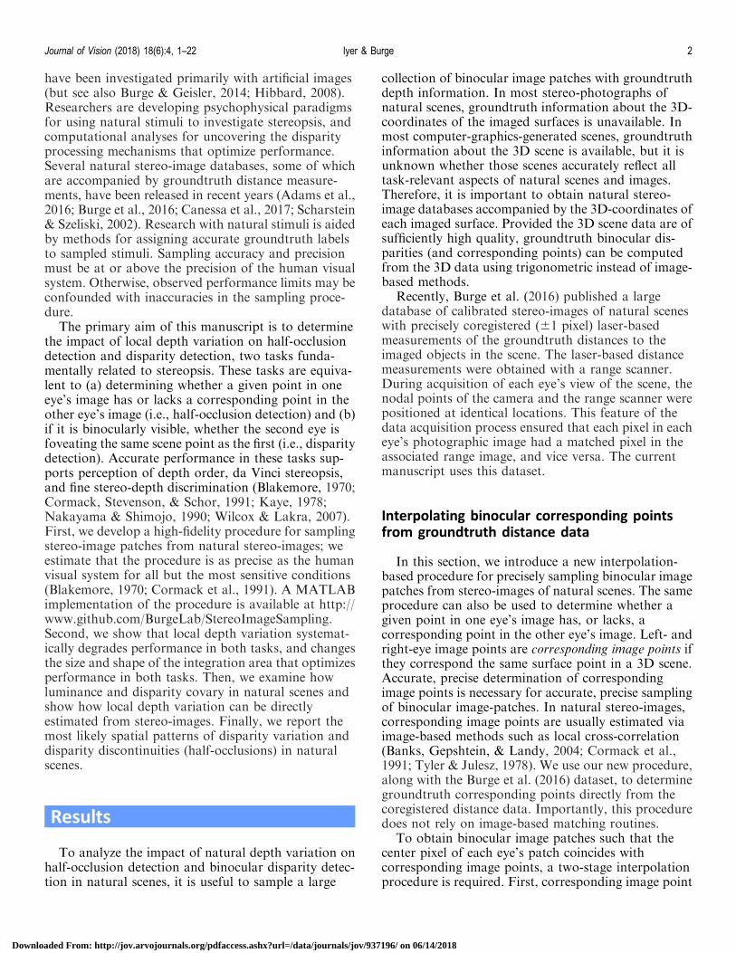
Sampling a pixel center from either the left- or theright-eye luminance image initializes the interpolationprocedure. The eye from whose image the pixel center isfirst chosen is the anchor eye. Each pixel is located in afrontoparallel projection plane 3 m from the cyclopeaneye (i.e., the midpoint of the interocular axis). Left-eye(LE) and right-eye (RE) lines of sight through thecenters of these pixels define a set of intersection pointsin 3D space (Figure 1A). These intersection points arethe sampled 3D scene points. When a point on a 3Dsurface coincides with a sampled 3D scene point, the

left- and right-eye lines of sight to this point intersectthe projection plane at pixel centers (Figure 1A).However, most sampled 3D scene points do not have a3D surface passing through them, and most 3D surfacepoints do not coincide with sampled 3D scene points.Thus, corresponding image points do not generallycoincide with pixel centers in the projection plane. Thegoal of our interpolation procedure is to interpolate 3Dsurface points and corresponding image points so thatthe postinterpolation pixel centers coincide withcorresponding image points

Figure 1B illustrates how interpolated 3D surfaceand corresponding image point locations are obtained.Consider a pair of LE and RE pixel centers thatcorrespond to a sampled 3D scene point. Sampled 3Dscene points (Figure 1B, open squares in scene) do notgenerally coincide with sampled 3D surface points

Figure 1. Stereo 3D sampling geometry, corresponding image-points, and interpolation procedure. (A) Top-view of 3D sampling

geometry. Left-eye (LE) and right-eye (RE) luminance and range images are captured one human interocular distance apart (65 mm).

Sampled 3D scene points (white squares) occur at the intersections of LE and RE lines of sight (thin lines) and usually do not lie on 3D

surfaces. Samples in the projection plane (i.e., pixel centers) are a subset of these sampled 3D scene points. Sampled 3D surface

points (white dots) occur at the intersections of LE or RE lines of sight with 3D surfaces (thick black curve) in the scene. Small arrows

along lines of sight represent light reflected from sampled 3D surface points that determine the pixel values in the luminance and

range images for each eye. Occasionally, sampled 3D surface points coincide with sampled 3D scene points (large dashed circles).

Light rays from these points intersect the projection plane at pixel centers. (B) Procedure to obtain corresponding image point

locations: Sample a pixel location (1) in the anchor eye’s image (here, the left eye). Locate the corresponding sampled left eye 3D

surface point (2). Find the right eye projection (3) from sampled 3D surface point by ray tracing. Select nearest pixel center (4) in right

eye image. Locate the corresponding sampled right eye 3D surface point (5). Find sampled 3D scene point (6) nearest the left- and

right-eye sampled 3D surface points. This sampled 3D scene point is the intersection point of the left- and right-eye lines of sight

through the sampled 3D surface points. Find interpolated 3D surface point (7) by linear interpolation (i.e., the location of the

intersection of cyclopean line of sight with chord joining sampled 3D surface points; see inset). Dashed light rays from this

interpolated 3D surface point define corresponding point locations (8) in the projection plane. The vergence demand h of the

interpolated scene point is the angle between the left- and right-eye lines of sight required to fixate the point. (C) Sampling error

before interpolation in arcmin. Dashed vertical lines indicate the expected sampling error assuming surface point locations are

uniformly distributed between sampled 3D scene points. (D) Estimated sampling error after interpolation in arcsec.



(Figure 1B, open circles). Thus, the luminance infor-mation in these pixels (Figure 1B, open squares inprojection plane) does not generally correspond to asingle point on a 3D surface. The interpolated surfacepoint (Figure 1B, black circle) occurs at the intersectionbetween the cyclopean line of sight and a line segmentconnecting sampled 3D surface points. This interpo-lated 3D surface point, unlike the sampled 3D scenepoint, lies on (or extremely near) a 3D surface. The LEand RE lines of sight to the interpolated 3D surfacepoint intersect the projection plane at correspondingimage points (Figure 1B, black squares).

This interpolation procedure is necessary to ensurethat binocular sampling errors are below humandisparity detection thresholds. Under optimal condi-tions, human disparity detection thresholds are ap-proximately 5 arcsec (Blakemore, 1970; Cormack et al.,1991). Failing to interpolate would result in 635 arcsecbinocular sampling errors (i.e., erroneous fixationdisparities), which are large relative to disparitydetection thresholds. Assuming that surfaces areuniformly distributed between sampled 3D scenepoints, the vergence demand difference of the interpo-lated 3D surface point and the nearest 3D sampledscene point should be uniformly distributed. Figure 1Cconfirms this prediction; the vergence demand differ-ences indeed tend to lie between 635 arcsec, indicatingthat the assumptions of the interpolation procedure are

valid. (Vergence demand h is the angle between the LEand RE lines of sight required fixating a given 3Dpoint; vergence demand difference Dh ¼ h2 � h1 is thedifference between two vergence demands.)

Unfortunately, interpolated corresponding imagepoints returned by this procedure are not guaranteed tobe true corresponding image points. If a sampledsurface point is half-occluded, then correspondingimage points do not exist, and the procedure returnsinvalid points. We screen for bad points by repeatingthe interpolation procedure twice, with a different eyeas anchor eye on each repeat. When interpolated 3Dsurface points from each anchor eye match, theirassociated vergence demands will match on bothrepeats, indicating that the interpolated correspondingpoints are valid. Figure 1D shows that after interpo-lation, approximately 80% of interpolated 3D surfacepoints had vergence demand differences of less than 65arcsec across repeats. For subsequent analyses ofbinocularly visible scene points, interpolated pointswith vergence demand differences larger than 65arcsec are discarded, ensuring that residual samplingerrors are smaller than human stereo-detection thresh-olds for all but the very most sensitive conditions(Blakemore, 1970; Cormack et al., 1991). Visualinspection of hundreds of interpolated points corrob-orates the numerical results.

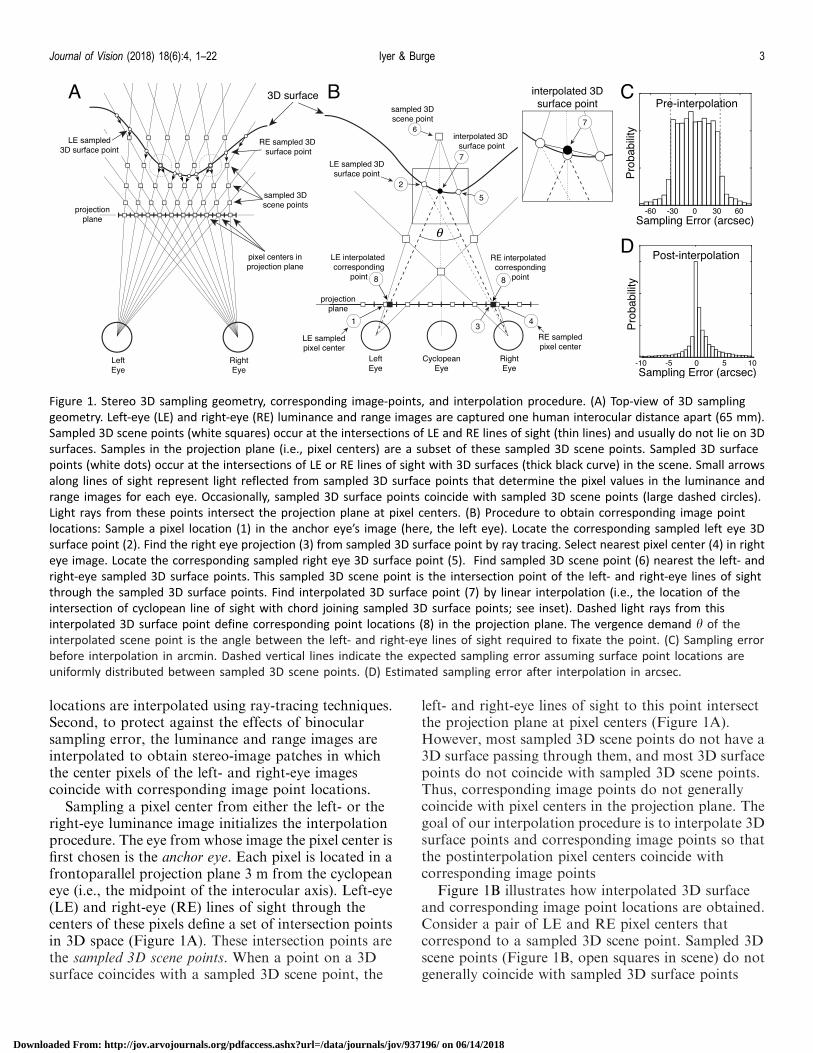
Figure 2. Half-occluded scene points, binocularly visible scene points, and vergence demand. (A) Half-occluded 3D surface point. The

scene point on the far surface (black circle) is visible to the left eye and occluded from the right eye. Arrows indicate the ray tracing

performed by the interpolation routine (see Figure 1). Squares represent interpolated image points returned by the interpolation

procedure. When 3D surface points are half-occluded, the interpolation procedure returns invalid points. (B) Binocularly visible

surface point (black circle) and corresponding image points (black squares) in the projection plane. When the scene point is

binocularly visible, the vergence demand h of the surface point is the same, regardless of the anchor eye. The vergence demand is

identical whether the left or the right eye is used as the anchor eye. (C) Vergence demand is computed within the epipolar plane

defined by a 3D surface point and the left- and right-eye nodal points.



To understand why half-occluded points can yieldinvalid corresponding image points, and why vergencedemand differences can help screen for them, considerthe scenario depicted in Figure 2A. When the left eye isthe anchor eye, the left-eye image point is associatedwith a far surface point having vergence demand hL,and the right-eye image point returned by theinterpolation is invalid because no true correspondingpoint exists. When the right eye is the anchor eye, thesame right-eye image point is associated with a nearsurface point having vergence demand hR not equal tohL. In other words, the vergence demand differenceDh ¼ hR � hL does not equal zero. Also note that whenthe right eye is the anchor eye, the left-eye image point(middle black square) returned by the procedure doesnot match the original left-eye image point. For cases in

which the surface point is binocularly visible, bothrepeats of the interpolation procedure yield the samevergence demands, surface points, and interpolatedimage points (Figure 2B). The vergence demand of asurface point is computed in the epipolar plane definedby the surface point and the left- and right-eye nodalpoints (Figure 2C).

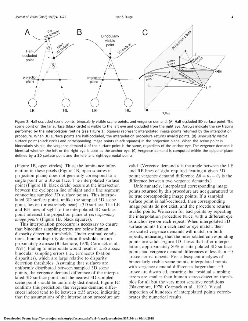
Results of the sampling and interpolation procedureare depicted in each of two natural scenes (Figure 3Aand B). Left- and right-eye luminance images (upperrow) and range images (lower row) are shown. 500randomly sampled corresponding image points, asso-ciated with 500 scene points, are overlaid onto eachstereo-image; 250 were sampled with the left eye as theanchor eye, and 250 were sampled with right eye as theanchor eye. Divergently-fuse the left two images or

Figure 3. Corresponding points overlaid on stereo-images (upper row) and coregistered groundtruth distance data (lower row) for two

different scenes, (A) and (B). Wall-fuse the left two images or cross-fuse the right two images to see the imaged scene in stereo-3D.

True corresponding points (yellow dots) lie on imaged 3D surfaces. Candidate corresponding points that are half-occluded or are

otherwise invalid (red dots) are also shown. For reference, the yellow boxes in (A) and (B) indicate 38 and 18 areas, respectively.



cross-fuse the right two images to see the scene and thecorresponding points in stereo-3D. True correspondingimage points (yellow) lie on the imaged surfaces in the3D scene. Invalid interpolated points (red) are alsoshown. To protect against eye-specific biases in thesubsequent analyses, surface points are sampled sym-metrically about the sagittal plane of the head.

After corresponding points are determined, lumi-nance and range values are interpolated on a uniformgrid of pixels centered at the corresponding points.Left- and right-eye luminance and range stereo- patchesare then cropped from the images. Maps of ground-truth disparity, relative to the center pixel, are thencomputed directly from the range images.

Quantifying local depth variation with disparitycontrast

The patterns of binocular disparities encountered bya behaving organism depend on the properties ofobjects in the environment and how the organisminteracts with those objects. When an organism fixatesa point on an object in a 3D scene, its image is formedon the left and right-eye foveas. These images are theinputs to the organism’s foveal disparity processingmechanisms. To a first approximation, if the fixatedpoint lies on a planar frontoparallel surface, thendisparities of nearby points will be zero. However,when the fixated point lies on curved, bumpy, and/orslanted surface, the disparities of nearby points willvary more significantly. When a depth edge is near thefixated point, dramatic changes in disparity can occurin the neighborhood of the fovea.

To quantify local depth variation, we compute thedisparity contrast associated with each stereo-pair thatis centered on a binocularly visible scene point.Disparity contrast is the root-mean-squared (RMS)disparity relative to the center pixel in a localneighborhood

Cd ¼

ffiffiffiffiffiffiffiffiffiffiffiffiffiffiffiffiffiffiffiffiffiffiffiffiffiffiffiffiXx2A

d xð Þ2,

N

vuut ð1Þ

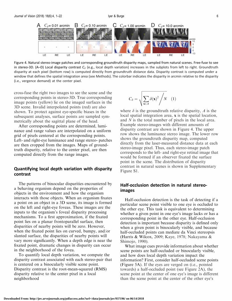
where d is the groundtruth relative disparity, A is thelocal spatial integration area, x is the spatial location,and N is the total number of pixels in the local area.Example stereo-images with different amounts ofdisparity contrast are shown in Figure 4. The upperrow shows the luminance stereo image. The lower rowshows the groundtruth disparity map, computeddirectly from the laser-measured distance data at eachstereo-image pixel. Thus, each stereo-image patchcorresponds to the left- and right-eye retinal image thatwould be formed if an observer fixated the surfacepoint in the scene. The distribution of disparitycontrast in natural scenes is shown in SupplementaryFigure S1.

Half-occlusion detection in natural stereo-images

Half-occlusion detection is the task of detecting if aparticular scene point visible to one eye is occluded tothe other eye. This task is equivalent to determiningwhether a given point in one eye’s image lacks or has acorresponding point in the other eye. Half-occlusiondetection is important because disparity is defined onlywhen a given point is binocularly visible, and becausehalf-occluded points can mediate da Vinci stereopsis(Harris & Wilcox, 2009; Kaye, 1978; Nakayama &Shimojo, 1990).

What image cues provide information about whetherscene points are half-occluded or binocularly visible,and how does local depth variation impact theinformation? First, consider half-occluded scene points(Figure 5A). If the eyes are verged on (i.e., pointedtowards) a half-occluded point (see Figure 2A), thescene point at the center of one eye’s image is differentthan the scene point at the center of the other eye’s

Figure 4. Natural stereo-image patches and corresponding groundtruth disparity maps, sampled from natural scenes. Free-fuse to see

in stereo-3D. (A–D) Local disparity contrast Cd (e.g., local depth variation) increases in the subplots from left to right. Groundtruth

disparity at each pixel (bottom row) is computed directly from groundtruth distance data. Disparity contrast is computed under a

window that defines the spatial integration area (see Methods). The colorbar indicates the disparity in arcmin relative to the disparity

(i.e., vergence demand) at the center pixel.



http://jov.arvojournals.org/data/Journals/JOV/937196/jovi-18-05-12_s02.pdf


image, the left- and right-eye images will be centered ondifferent points in the scene, and the left- and right-eyeimages should be very different (Figure 5B). Now,consider binocularly visible scene points. If the eyes areverged (i.e., fixated) on a binocularly visible scenepoint, the left- and right-eye images should be verysimilar. However, if local depth variation near abinocularly visible scene point is high, left- and right-eye images centered on that point should be less similar.

To examine the impact of local disparity variation onhalf-occlusion detection in natural scenes, we firstsampled 10,000 stereo-image patches from the naturalscene database using the procedure discussed above.We found that 86.5% of the sampled stereo-image pairswere centered on binocularly visible scene points, andthat 13.5% were centered on half-occluded scene points.We determined which patches had half-occludedcenters directly from the range measurements bydetermining which patches had centers where thehorizontal disparity gradient (DG ¼ Dh=DX) with anyother point was 2.0 or higher (a disparity gradient of2.0 corresponds to Panum’s limiting case; see Bulthoff,Fahle, & Wegmann, 1991). The disparity gradient inthe half-occlusion scenario depicted in Figure 2A issomewhat larger than 2.0. Second, to quantify local

depth variation, we computed the disparity contrast ofall patches with binocularly visible centers. For allanalyses, disparity contrast was computed over a localintegration area of 1.08 (0.58 full-width at half-height;see Equation 1); results are robust to this choice (seeSupplementary Figure S1). Third, the similarity of theleft- and right-eye image patches was quantified withthe correlation coefficient

qLR ¼

Px2A

cWL xð ÞcWR xð Þ

cWL xð Þ�� cWR xð Þ

�� ð2Þ

where cWL and cWR are windowed left- and right-eyeWeber contrast images (see Methods) and where

c xð Þk k ¼ffiffiffiffiffiffiffiffiffiffiffiffiffiffiffiffiffiffiffiffiffiffiffiPN

x2A c xð Þ2q

is the L2 norm of the contrast

image in a local integration area A. The integrationarea is determined by the size of a cosine windowingfunction W (see Methods); the windowing functiondetermines the size of the spatial integration area withinwhich binocular correlation is computed. Fourth,under the assumption that the correlation coefficient isthe decision variable, we used standard methods fromsignal detection theory to determine how well half-occlusions can be detected in natural images. Specifi-

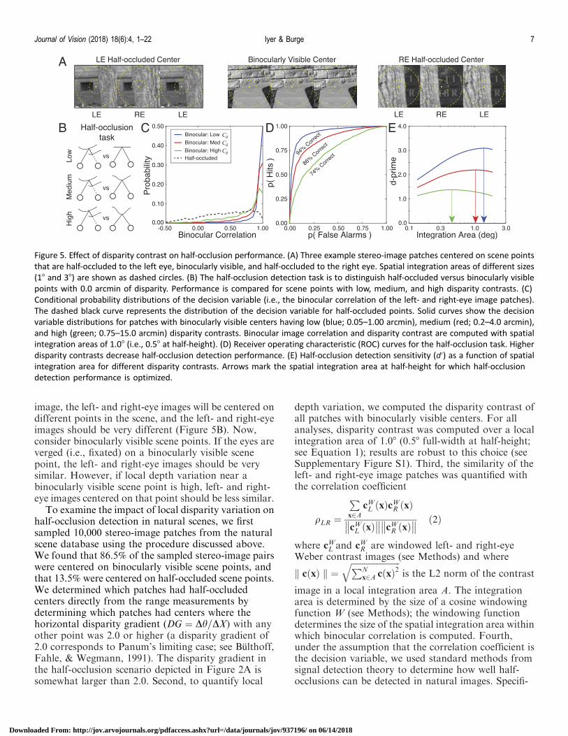
Figure 5. Effect of disparity contrast on half-occlusion performance. (A) Three example stereo-image patches centered on scene points

that are half-occluded to the left eye, binocularly visible, and half-occluded to the right eye. Spatial integration areas of different sizes

(18 and 38) are shown as dashed circles. (B) The half-occlusion detection task is to distinguish half-occluded versus binocularly visible

points with 0.0 arcmin of disparity. Performance is compared for scene points with low, medium, and high disparity contrasts. (C)

Conditional probability distributions of the decision variable (i.e., the binocular correlation of the left- and right-eye image patches).

The dashed black curve represents the distribution of the decision variable for half-occluded points. Solid curves show the decision

variable distributions for patches with binocularly visible centers having low (blue; 0.05–1.00 arcmin), medium (red; 0.2–4.0 arcmin),

and high (green; 0.75–15.0 arcmin) disparity contrasts. Binocular image correlation and disparity contrast are computed with spatial

integration areas of 1.08 (i.e., 0.58 at half-height). (D) Receiver operating characteristic (ROC) curves for the half-occlusion task. Higher

disparity contrasts decrease half-occlusion detection performance. (E) Half-occlusion detection sensitivity (d0) as a function of spatial

integration area for different disparity contrasts. Arrows mark the spatial integration area at half-height for which half-occlusion

detection performance is optimized.




cally, we determined the conditional probability of thedecision variable given (a) that the center pixel wasbinocularly visible for each disparity contrastp qLRjbino;Cdð Þ and (b) that the center pixel was half-occluded p qLRjmonoð Þ (Figure 5C), swept out an ROCcurve (Figure 5D), computed the area underneath it todetermine percent correct, and then converted to d0.Finally, we repeated the steps for different spatialintegration areas. Half-occlusion detection perfor-mance (d0) changes significantly as a function of thespatial integration area for each of several disparitycontrasts (Figure 5E). Clearly, local depth variationreduces how well binocularly visible points can bediscriminated from half-occluded points. (Note that thesame procedure could be adapted to work in the retinalperiphery with one straightforward extension. For anygiven patch in one eye’s image, a cross-correlationcould be performed to determine the peripherallocations in the other eye to compare. The correlationof the two patches yielding the maximum correlationcould then be used as input to the procedure describedabove.)

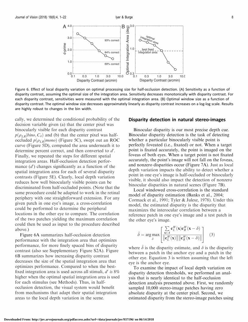
Figure 6A summarizes half-occlusion detectionperformance with the integration area that optimizesperformance, for more finely spaced bins of disparitycontrast (also see Supplementary Figure S2A). Figure6B summarizes how increasing disparity contrastdecreases the size of the spatial integration area thatoptimizes performance. Compared to when the best-fixed integration area is used across all stimuli, d0 is 8%higher when the optimal spatial integration area is usedfor each stimulus (see Methods). Thus, in half-occlusion detection, the visual system would benefitfrom mechanisms that adapt their spatial integrationareas to the local depth variation in the scene.

Disparity detection in natural stereo-images

Binocular disparity is our most precise depth cue.Binocular disparity detection is the task of detectingwhether a particular binocularly visible point isperfectly foveated (i.e., fixated) or not. When a targetpoint is fixated accurately, the point is imaged on thefoveas of both eyes. When a target point is not fixatedaccurately, the point’s image will not fall on the foveas,and nonzero disparities occur (Figure 7A). Just as localdepth variation impacts the ability to detect whether apoint in one eye’s image is half-occluded or binocularlyvisible, it should also impact the detection of nonzerobinocular disparities in natural scenes (Figure 7B).

Local windowed cross-correlation is the standardmodel of disparity estimation (Banks et al., 2004;Cormack et al., 1991; Tyler & Julesz, 1978). Under thismodel, the estimated disparity is the disparity thatmaximizes the interocular correlation between areference patch in one eye’s image and a test patch inthe other eye’s image.

d ¼ arg maxd

Px2A

cWL xð ÞcWR x� dð Þ

cWL xð Þ�� cWR x� dð Þ

�� 24

35 ð3Þ

where d is the disparity estimate, and d is the disparitybetween a patch in the anchor eye and a patch in theother eye. Equation 3 is written assuming that the lefteye is the anchor eye.

To examine the impact of local depth variation ondisparity detection thresholds, we performed an anal-ysis that is nearly identical to the half-occlusiondetection analysis presented above. First, we randomlysampled 10,000 stereo-image patches having zeroabsolute disparity at the center pixel. Second, weestimated disparity from the stereo-image patches using

Figure 6. Effect of local disparity variation on optimal processing size for half-occlusion detection. (A) Sensitivity as a function of

disparity contrast, assuming the optimal size of the integration area. Sensitivity decreases monotonically with disparity contrast. For

each disparity contrast, sensitivities were measured with the optimal integration area. (B) Optimal window size as a function of

disparity contrast. The optimal window size decreases approximately linearly as disparity contrast increases on a log-log scale. Results

are highly robust to changes in the bin width.




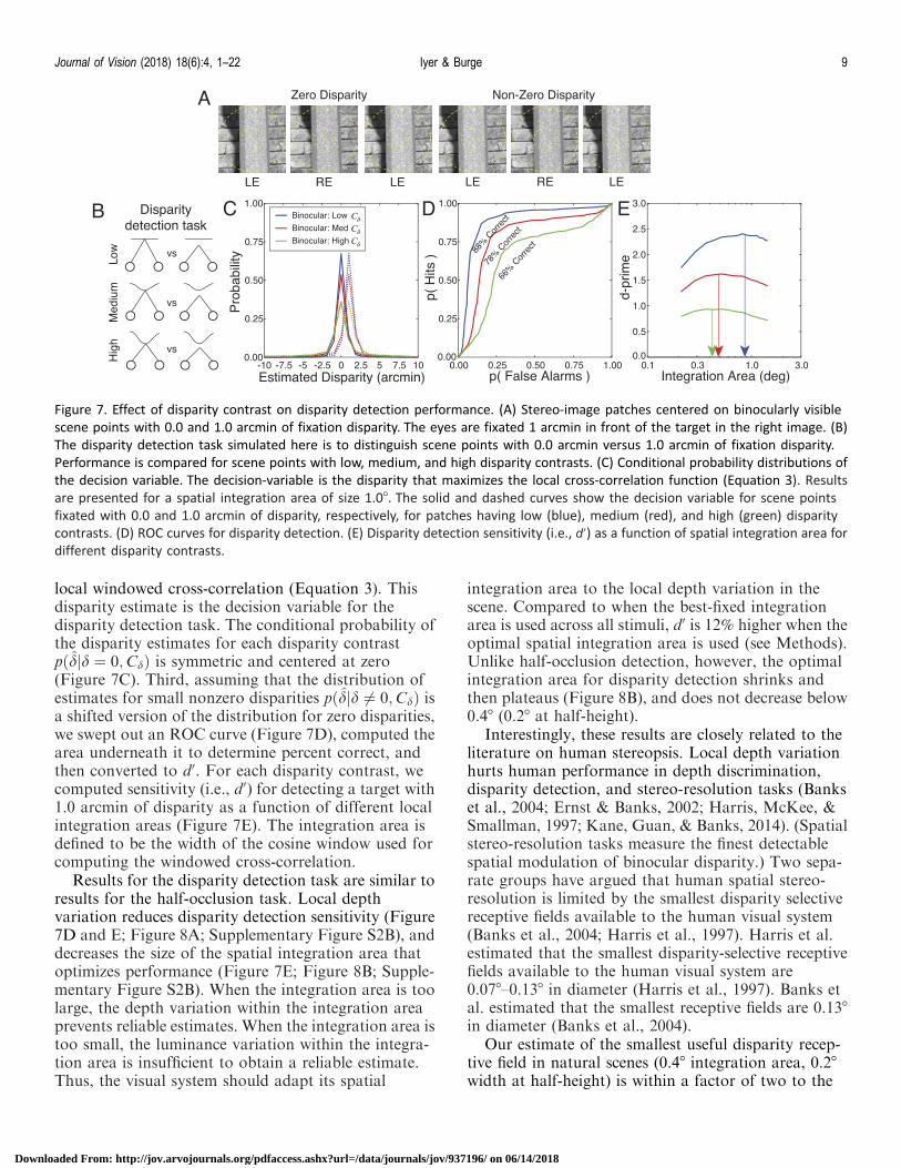
local windowed cross-correlation (Equation 3). Thisdisparity estimate is the decision variable for thedisparity detection task. The conditional probability ofthe disparity estimates for each disparity contrastpðdjd ¼ 0;CdÞ is symmetric and centered at zero(Figure 7C). Third, assuming that the distribution ofestimates for small nonzero disparities pðdjd 6¼ 0;CdÞ isa shifted version of the distribution for zero disparities,we swept out an ROC curve (Figure 7D), computed thearea underneath it to determine percent correct, andthen converted to d0. For each disparity contrast, wecomputed sensitivity (i.e., d0) for detecting a target with1.0 arcmin of disparity as a function of different localintegration areas (Figure 7E). The integration area isdefined to be the width of the cosine window used forcomputing the windowed cross-correlation.

Results for the disparity detection task are similar toresults for the half-occlusion task. Local depthvariation reduces disparity detection sensitivity (Figure7D and E; Figure 8A; Supplementary Figure S2B), anddecreases the size of the spatial integration area thatoptimizes performance (Figure 7E; Figure 8B; Supple-mentary Figure S2B). When the integration area is toolarge, the depth variation within the integration areaprevents reliable estimates. When the integration area istoo small, the luminance variation within the integra-tion area is insufficient to obtain a reliable estimate.Thus, the visual system should adapt its spatial

integration area to the local depth variation in thescene. Compared to when the best-fixed integrationarea is used across all stimuli, d0 is 12% higher when theoptimal spatial integration area is used (see Methods).Unlike half-occlusion detection, however, the optimalintegration area for disparity detection shrinks andthen plateaus (Figure 8B), and does not decrease below0.48 (0.28 at half-height).

Interestingly, these results are closely related to theliterature on human stereopsis. Local depth variationhurts human performance in depth discrimination,disparity detection, and stereo-resolution tasks (Bankset al., 2004; Ernst & Banks, 2002; Harris, McKee, &Smallman, 1997; Kane, Guan, & Banks, 2014). (Spatialstereo-resolution tasks measure the finest detectablespatial modulation of binocular disparity.) Two sepa-rate groups have argued that human spatial stereo-resolution is limited by the smallest disparity selectivereceptive fields available to the human visual system(Banks et al., 2004; Harris et al., 1997). Harris et al.estimated that the smallest disparity-selective receptivefields available to the human visual system are0.078–0.138 in diameter (Harris et al., 1997). Banks etal. estimated that the smallest receptive fields are 0.138in diameter (Banks et al., 2004).

Our estimate of the smallest useful disparity recep-tive field in natural scenes (0.48 integration area, 0.28

width at half-height) is within a factor of two to the

Figure 7. Effect of disparity contrast on disparity detection performance. (A) Stereo-image patches centered on binocularly visible

scene points with 0.0 and 1.0 arcmin of fixation disparity. The eyes are fixated 1 arcmin in front of the target in the right image. (B)

The disparity detection task simulated here is to distinguish scene points with 0.0 arcmin versus 1.0 arcmin of fixation disparity.

Performance is compared for scene points with low, medium, and high disparity contrasts. (C) Conditional probability distributions of

the decision variable. The decision-variable is the disparity that maximizes the local cross-correlation function (Equation 3). Results

are presented for a spatial integration area of size 1.08. The solid and dashed curves show the decision variable for scene points

fixated with 0.0 and 1.0 arcmin of disparity, respectively, for patches having low (blue), medium (red), and high (green) disparity

contrasts. (D) ROC curves for disparity detection. (E) Disparity detection sensitivity (i.e., d0) as a function of spatial integration area for

different disparity contrasts.






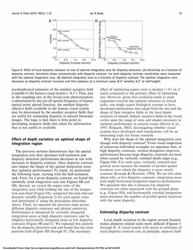
psychophysical estimates of the smallest receptive fieldavailable to the human visual system (;0.18). Thus, justas the sampling rate of the foveal cone photoreceptorsis determined by the cut-off spatial frequency of humanoptical point spread function, the smallest disparityselective fields available to the human visual systemmay be determined by the smallest receptive fields thatare useful for estimating disparity in natural binocularimages. The logic is that there is little point indeveloping receptive fields that select for informationthat is not useful or available.

Effect of depth variation on optimal shape ofintegration region

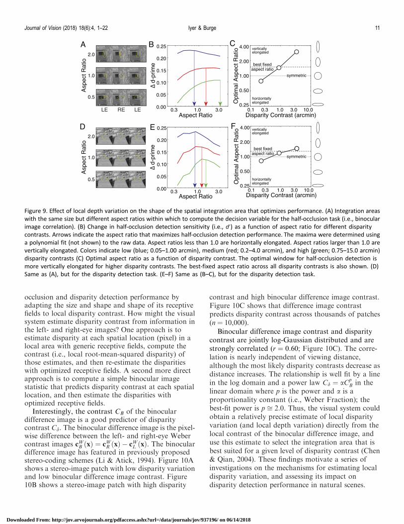
The previous sections demonstrate that the spatialintegration area that optimizes half-occlusion anddisparity detection performance decreases in size withincreases in disparity contrast. Does disparity contrastalso impact the shape of the spatial integration areasthat optimize performance? To check, we performedthe following steps, starting with the half-occlusiontask. First, for a given disparity contrast, we found theoptimally sized integration area (see Figures 6B and8B). Second, we varied the aspect ratio of theintegration area while holding the size of the integra-tion area fixed (Figure 9A), computed the task-relevantdecision variable (Equation 2) for each aspect ratio,and determined d0 using the procedures describedabove. Third, we repeated the previous steps acrossdifferent disparity contrasts and plotted sensitivity.Performance is optimized by vertically elongatedintegration areas at high disparity contrasts, and by(slightly) horizontally elongated areas at low disparitycontrasts (Figure 9B and C). We repeated this analysisfor the disparity detection task and found that the samepatterns hold (Figure 9D through F). The secondary

effect of optimizing aspect ratio is modest (;0.1 in d0

units) compared to the primary effect of optimizingsize. However, given that evolution tends to pushorganisms towards the optimal solutions in criticaltasks, one might expect biological systems to havedeveloped mechanisms that adapt both the size and theshape of their receptive fields to the local depthstructure of stimuli. Indeed, receptive fields in the visualcortex span the range of sizes and shapes necessary tooptimize performance in natural scenes (Harris et al.,1997; Ringach, 2002). Investigating whether visualsystems have developed such mechanisms will be aninteresting topic for future research.

Why does the shape of the optimal integration areachange with disparity contrast? From visual inspectionof numerous individual examples we speculate that, athigh disparity contrasts, vertical elongation improvesperformance because large disparity contrasts are mostoften caused by vertically oriented depth edges (e.g.,Figure 9A). For such cases, vertically oriented inte-gration areas increase the number of pooled spatiallocations over which the disparity is more nearlyconstant (Kanade & Okutomi, 1994). We are less clearabout why, at low disparity contrasts, integration areaswith slight horizontal elongation improve performance.We speculate that this is because low disparitycontrasts are often associated with the ground plane(e.g., Figure 9D), and horizontally oriented integrationareas maximize the number of pooled spatial locationswith the same disparity.

Estimating disparity contrast

Local depth variation in the region around fixationmakes disparity-related tasks more difficult (Figures 5through 8). A visual system with access to estimates oflocal disparity contrast can, in principle, improve half-

Figure 8. Effect of local disparity variation on size of optimal integration area for disparity detection. (A) Sensitivity as a function of

disparity contrast. Sensitivity drops monotonically with disparity contrast. For each disparity contrast, sensitivities were measured

with the optimal integration area. (B) Optimal integration area as a function of disparity contrast. The optimal integration area

decreases as disparity contrast increases and then plateaus at a minimum value (0.48 window; 0.28 at half-height).



occlusion and disparity detection performance byadapting the size and shape and shape of its receptivefields to local disparity contrast. How might the visualsystem estimate disparity contrast from information inthe left- and right-eye images? One approach is toestimate disparity at each spatial location (pixel) in alocal area with generic receptive fields, compute thecontrast (i.e., local root-mean-squared disparity) ofthose estimates, and then re-estimate the disparitieswith optimized receptive fields. A second more directapproach is to compute a simple binocular imagestatistic that predicts disparity contrast at each spatiallocation, and then estimate the disparities withoptimized receptive fields.

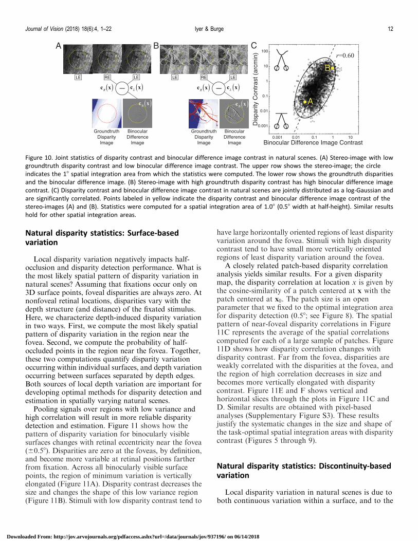
Interestingly, the contrast CB of the binoculardifference image is a good predictor of disparitycontrast Cd. The binocular difference image is the pixel-wise difference between the left- and right-eye Webercontrast images cWB xð Þ ¼ cWR xð Þ � cWL xð Þ. The binoculardifference image has featured in previously proposedstereo-coding schemes (Li & Atick, 1994). Figure 10Ashows a stereo-image patch with low disparity variationand low binocular difference image contrast. Figure10B shows a stereo-image patch with high disparity

contrast and high binocular difference image contrast.Figure 10C shows that difference image contrastpredicts disparity contrast across thousands of patches(n ¼ 10,000).

Binocular difference image contrast and disparitycontrast are jointly log-Gaussian distributed and arestrongly correlated (r ¼ 0:60; Figure 10C). The corre-lation is nearly independent of viewing distance,although the most likely disparity contrasts decrease asdistance increases. The relationship is well fit by a linein the log domain and a power law Cd ¼ aCp

B in thelinear domain where p is the power and a is aproportionality constant (i.e., Weber Fraction); thebest-fit power is p ffi 2:0. Thus, the visual system couldobtain a relatively precise estimate of local disparityvariation (and local depth variation) directly from thelocal contrast of the binocular difference image, anduse this estimate to select the integration area that isbest suited for a given level of disparity contrast (Chen& Qian, 2004). These findings motivate a series ofinvestigations on the mechanisms for estimating localdisparity variation, and assessing its impact ondisparity detection performance in natural scenes.

Figure 9. Effect of local depth variation on the shape of the spatial integration area that optimizes performance. (A) Integration areas

with the same size but different aspect ratios within which to compute the decision variable for the half-occlusion task (i.e., binocular

image correlation). (B) Change in half-occlusion detection sensitivity (i.e., d0) as a function of aspect ratio for different disparity

contrasts. Arrows indicate the aspect ratio that maximizes half-occlusion detection performance. The maxima were determined using

a polynomial fit (not shown) to the raw data. Aspect ratios less than 1.0 are horizontally elongated. Aspect ratios larger than 1.0 are

vertically elongated. Colors indicate low (blue; 0.05–1.00 arcmin), medium (red; 0.2–4.0 arcmin), and high (green; 0.75–15.0 arcmin)

disparity contrasts (C) Optimal aspect ratio as a function of disparity contrast. The optimal window for half-occlusion detection is

more vertically elongated for higher disparity contrasts. The best-fixed aspect ratio across all disparity contrasts is also shown. (D)

Same as (A), but for the disparity detection task. (E–F) Same as (B–C), but for the disparity detection task.



Natural disparity statistics: Surface-basedvariation

Local disparity variation negatively impacts half-occlusion and disparity detection performance. What isthe most likely spatial pattern of disparity variation innatural scenes? Assuming that fixations occur only on3D surface points, foveal disparities are always zero. Atnonfoveal retinal locations, disparities vary with thedepth structure (and distance) of the fixated stimulus.Here, we characterize depth-induced disparity variationin two ways. First, we compute the most likely spatialpattern of disparity variation in the region near thefovea. Second, we compute the probability of half-occluded points in the region near the fovea. Together,these two computations quantify disparity variationoccurring within individual surfaces, and depth variationoccurring between surfaces separated by depth edges.Both sources of local depth variation are important fordeveloping optimal methods for disparity detection andestimation in spatially varying natural scenes.

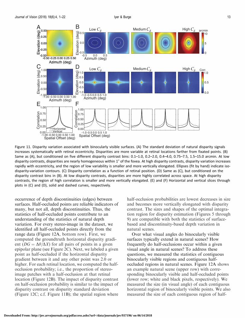
Pooling signals over regions with low variance andhigh correlation will result in more reliable disparitydetection and estimation. Figure 11 shows how thepattern of disparity variation for binocularly visiblesurfaces changes with retinal eccentricity near the fovea(60.58). Disparities are zero at the foveas, by definition,and become more variable at retinal positions fartherfrom fixation. Across all binocularly visible surfacepoints, the region of minimum variation is verticallyelongated (Figure 11A). Disparity contrast decreases thesize and changes the shape of this low variance region(Figure 11B). Stimuli with low disparity contrast tend to

have large horizontally oriented regions of least disparityvariation around the fovea. Stimuli with high disparitycontrast tend to have small more vertically orientedregions of least disparity variation around the fovea.

A closely related patch-based disparity correlationanalysis yields similar results. For a given disparitymap, the disparity correlation at location x is given bythe cosine-similarity of a patch centered at x with thepatch centered at x0. The patch size is an openparameter that we fixed to the optimal integration areafor disparity detection (0.58; see Figure 8). The spatialpattern of near-foveal disparity correlations in Figure11C represents the average of the spatial correlationscomputed for each of a large sample of patches. Figure11D shows how disparity correlation changes withdisparity contrast. Far from the fovea, disparities areweakly correlated with the disparities at the fovea, andthe region of high correlation decreases in size andbecomes more vertically elongated with disparitycontrast. Figure 11E and F shows vertical andhorizontal slices through the plots in Figure 11C andD. Similar results are obtained with pixel-basedanalyses (Supplementary Figure S3). These resultsjustify the systematic changes in the size and shape ofthe task-optimal spatial integration areas with disparitycontrast (Figures 5 through 9).

Natural disparity statistics: Discontinuity-basedvariation

Local disparity variation in natural scenes is due toboth continuous variation within a surface, and to the

Figure 10. Joint statistics of disparity contrast and binocular difference image contrast in natural scenes. (A) Stereo-image with low

groundtruth disparity contrast and low binocular difference image contrast. The upper row shows the stereo-image; the circle

indicates the 18 spatial integration area from which the statistics were computed. The lower row shows the groundtruth disparities

and the binocular difference image. (B) Stereo-image with high groundtruth disparity contrast has high binocular difference image

contrast. (C) Disparity contrast and binocular difference image contrast in natural scenes are jointly distributed as a log-Gaussian and

are significantly correlated. Points labeled in yellow indicate the disparity contrast and binocular difference image contrast of the

stereo-images (A) and (B). Statistics were computed for a spatial integration area of 1.08 (0.58 width at half-height). Similar results

hold for other spatial integration areas.




occurrence of depth discontinuities (edges) betweensurfaces. Half-occluded points are reliable indicators ofmany, but not all, depth discontinuities. Thus, thestatistics of half-occluded points contribute to anunderstanding of the statistics of natural depthvariation. For every stereo-image in the dataset, weidentified all half-occluded points directly from therange data (Figure 12A, bottom row). First, wecomputed the groundtruth horizontal disparity gradi-ent (DG ¼ Dh=DX) for all pairs of points in a givenepipolar plane (see Figure 2C). Next, we labeled a givenpoint as half-occluded if the horizontal disparitygradient between it and any other point was 2.0 orhigher. For each retinal location, we computed the half-occlusion probability; i.e., the proportion of stereo-image patches with a half-occlusion at that retinallocation (Figure 12B). The impact of disparity contraston half-occlusion probability is similar to the impact ofdisparity contrast on disparity standard deviation(Figure 12C; c.f. Figure 11B); the spatial region where

half-occlusion probabilities are lowest decreases in sizeand becomes more vertically elongated with disparitycontrast. The sizes and shapes of the optimal integra-tion region for disparity estimation (Figures 5 through9) are compatible with both the statistics of surface-based and discontinuity-based depth variation innatural scenes.

Over what visual angles do binocularly visiblesurfaces typically extend in natural scenes? Howfrequently do half-occlusions occur within a givenvisual angle in natural scenes? To address thesequestions, we measured the statistics of contiguousbinocularly visible regions and contiguous half-occluded regions in natural scenes. Figure 12A showsan example natural scene (upper row) with corre-sponding binocularly visible and half-occluded points(lower row; white and black pixels, respectively). Wemeasured the size (in visual angle) of each contiguoushorizontal region of binocularly visible points. We alsomeasured the size of each contiguous region of half-

Figure 11. Disparity variation associated with binocularly visible surfaces. (A) The standard deviation of natural disparity signals

increases systematically with retinal eccentricity. Disparities are more variable at retinal locations farther from fixated points. (B)

Same as (A), but conditioned on five different disparity contrast bins: 0.1–1.0, 0.2–2.0, 0.4–4.0, 0.75–7.5, 1.5–15.0 arcmin. At low

disparity contrasts, disparities are nearly homogeneous within 18 of the fovea. At high disparity contrasts, disparity variation increases

rapidly with eccentricity, and the region of low variability is smaller and more vertically elongated. Ellipses (fit by hand) indicate iso-

disparity-variation contours. (C) Disparity correlation as a function of retinal position. (D) Same as (C), but conditioned on the

disparity contrast bins in (B). At low disparity contrasts, disparities are more highly correlated across space. At high disparity

contrasts, the region of high correlation is smaller and more vertically elongated. (E) and (F) Horizontal and vertical slices through

plots in (C) and (D), solid and dashed curves, respectively.



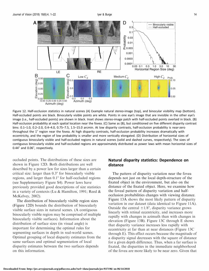
occluded points. The distributions of these sizes areshown in Figure 12D. Both distributions are welldescribed by a power law for sizes larger than a certaincritical size: larger than 0.38 for binocularly visibleregions, and larger than 0.18 for half-occluded regions(see Supplementary Figure S4). Power laws havepreviously provided good descriptions of size statisticsin a variety of contexts (Lu & Hamilton, 1991; Reed &McKelvey, 2002).

The distribution of binocularly visible region sizes(Figure 12D) bounds the distribution of binocularlyvisible surface sizes in natural scenes. (A contiguousbinocularly visible region may be comprised of multiplebinocularly visible surfaces). Information about thedistribution of surface sizes (in visual angle) isimportant for determining the optimal rules forsegmenting surfaces in depth in real-world scenes.Optimal grouping of local disparity estimates from thesame surfaces and optimal segmentation of localdisparity estimates between the two surfaces dependson this information.

Natural disparity statistics: Dependence ondistance

The pattern of disparity variation near the foveadepends not just on the local depth-structure of thefixated object in the environment, but also on thedistance of the fixated object. Here, we examine howthe foveal pattern of disparity variation and half-occlusion probabilities changes with viewing distance.Figure 13A shows the most likely pattern of disparityvariation in our dataset (data identical to Figure 11A).Outside the central 61/88, disparity variance growslinearly with retinal eccentricity, and increases morerapidly with changes in azimuth than with changes inelevation (Figure 13B). Figure 13C through E showsthat disparity variance increases less rapidly witheccentricity at far than at near distances (Figure 13Cthrough E). This effect occurs because the magnitude ofa disparity signal decreases with the square of distancefor a given depth difference. Thus, when a far surface isfixated, the disparities in the immediate neighborhoodof the fovea are more likely to be near zero. Given that

Figure 12. Half-occlusion statistics in natural scenes (A) Example natural stereo-image (top), and binocular visibility map (bottom).

Half-occluded points are black. Binocularly visible points are white. Points in one eye’s image that are invisible in the other eye’s

image (i.e., half-occluded points) are shown in black. Inset shows stereo-image patch with half-occluded points overlaid in black. (B)

Half-occlusion probability at each spatial location near the fovea. (C) Same as (B), but conditioned on five different disparity contrast

bins: 0.1–1.0, 0.2–2.0, 0.4–4.0, 0.75–7.5, 1.5–15.0 arcmin. At low disparity contrasts, half-occlusion probability is near-zero

throughout the 18 region near the fovea. At high disparity contrasts, half-occlusion probability increases dramatically with

eccentricity, and the region of low probability is smaller and more vertically elongated. (D) Distribution of horizontal sizes of

contiguous binocularly visible and half-occluded regions in natural scenes (solid and dashed curves, respectively). The sizes of

contiguous binocularly visible and half-occluded regions are approximately distributed as power laws with mean horizontal sizes of

0.448 and 0.068, respectively.




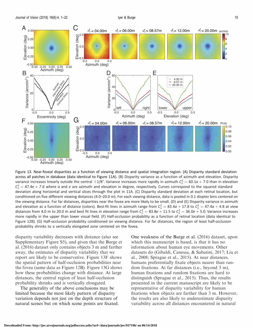
disparity variability decreases with distance (also seeSupplementary Figure S5), and given that the Burge etal. (2016) dataset only contains objects 3 m and fartheraway, the estimates of disparity variability that wereport are likely to be conservative. Figure 13F showsthe spatial pattern of half-occlusion probabilities nearthe fovea (same data as Figure 12B). Figure 13G showshow these probabilities change with distance. At largedistances, the central region of least half-occlusionprobability shrinks and is vertically elongated.

The generality of the above conclusions may belimited because the most likely pattern of disparityvariation depends not just on the depth structure ofnatural scenes but on which scene points are fixated.

One weakness of the Burge et al. (2016) dataset, uponwhich this manuscript is based, is that it has noinformation about human eye movements. Otherdatasets do (Gibaldi, Canessa, & Sabatini, 2017; Liu etal., 2008; Sprague et al., 2015). At near distances,humans preferentially fixate objects nearer than ran-dom fixations. At far distances (i.e., beyond 3 m),human fixations and random fixations are hard todistinguish (Sprague et al., 2015). Thus, the resultspresented in the current manuscript are likely to berepresentative of disparity variability for humanfixations when objects are farther than 3 m. However,the results are also likely to underestimate disparityvariability across all distances encountered in natural

Figure 13. Near-foveal disparities as a function of viewing distance and spatial integration region. (A) Disparity standard deviation

across all patches in database (data identical to Figure 11A). (B) Disparity variance as a function of azimuth and elevation. Disparity

variance increases linearly outside the central 61/88. Variance increases more rapidly in azimuth C2d ¼ 60:1aþ 7:0 than in elevation

C2d ¼ 47:4eþ 7:6 where a and e are azimuth and elevation in degree, respectively. Curves correspond to the squared standard

deviation along horizontal and vertical slices through the plot in 11A. (C) Disparity standard deviation at each retinal location, but

conditioned on five different viewing distances (4.0–20.0 m). For each viewing distance, data is pooled in 0.1 diopter bins centered on

the viewing distance. For far distances, disparities near the fovea are more likely to be small. (D) and (E) Disparity variance in azimuth

and elevation as a function of distance (colors). Best-fit lines in azimuth range from C2d ¼ 83:4aþ 17:8 to C2

d ¼ 47:4aþ 4:8 at view

distances from 4.0 m to 20.0 m and best fit lines in elevation range from C2d ¼ 83:8eþ 11:5 to C2

d ¼ 36:0eþ 5:0. Variance increases

more rapidly in the upper than lower visual field. (F) Half-occlusion probability as a function of retinal location (data identical to

Figure 12B). (G) Half-occlusion probability conditioned on viewing distance. For far distances, the region of least half-occlusion

probability shrinks to a vertically elongated zone centered on the fovea.




viewing (also see Supplementary Figure S1 andSupplementary Figure S6).

Discussion

We developed a high-precision stereo-image sam-pling procedure, and used it along with a recentlypublished dataset (Burge et al., 2016), to demonstratehow natural depth variation impacts performance intwo tasks fundamentally related to stereopsis. In thefirst set of analyses, we analyzed natural binocularimages and determined the receptive field sizes andshapes that optimize performance in half-occlusiondetection and disparity detection in natural scenes. Inthe second set of analyses, we analyzed groundtruthrange data and determined how disparity statistics andhalf-occlusion probabilities change as a function ofretinal eccentricity. The latter analyses justify thefindings of the former. Here, in the discussion section,we discuss the connections to other topics in theliterature, limitations of the current results, anddirections for future work.

Relationship to previous work

The dataset leveraged in this manuscript has someadvantages and some disadvantages compared to otherrecently published datasets. We compare four recentlypublished datasets, and consider the advantages anddisadvantages of each with respect to six factors: (a) thepresence or absence of eye movements, (b) the presenceor absence of groundtruth half-occlusions andgroundtruth disparities, (c) the spatial resolution of theimages, (d) the range of object distances represented inthe dataset, (e) the diversity of the sampled scenes, and(f) the appropriateness of the dataset for use inpsychophysical experiments. Each dataset was collectedwith a different purpose (or set of purposes) in mind,and each is limited by choices made by the researchersand by the technology used to collect the data.

Sprague et al. (2015) affixed human observers with amobile binocular eye tracker and collected binocularimage movies of natural scenes as human observersperformed everyday tasks around the University ofCalifornia, Berkeley. The dataset contains objectsranging in distance from 0.5 m to infinity. The principalaim in collecting the dataset was to estimate the priorprobability distribution of binocular disparities en-countered by humans in natural viewing. Absolutedisparity depends on the 3D structure of the scene,where the observer is located in the scene, and wherethe observer gazes in the scene. Collecting stereo-images in concert with matched binocular eye move-

ments is therefore necessary to estimate the distributionof disparities encountered by humans, and the datasetis well suited for this aim. There are two primarydisadvantages associated with the dataset. The firstdisadvantage is that groundtruth disparities andgroundtruth occlusions are not known. Disparitieswere instead estimated from the left- and right-eyeimages via image-based routines. A second disadvan-tage is that the stereo-images are low spatial resolution(;9 pix/deg). Thus, while this dataset is well-suited forestimating disparity statistics in natural viewing, it is ill-suited for examining the accuracy of disparity estima-tion algorithms, for investigating the impact of localdisparity variation on disparity estimation perfor-mance, or for obtaining natural stimuli for use inpsychophysical experiments.

Gibaldi et al. (2017) tracked binocular eye move-ments of head-fixed human observers viewing twocomputer generated 3D scenes from different view-points on a stereo-display (Gibaldi et al., 2017). Thedataset contains objects ranging in distance from only0.5 to 1.5 m. This paper also had the aim ofcharacterizing disparity statistics in natural viewing.Gibaldi et al.’s computer-generated scenes afford accessto groundtruth disparities and groundtruth occlusions.The rendered images had comparatively high spatialresolution (;44 pix/deg) and, with appropriate cali-bration, could be suitable for use in psychophysicalexperiments. All of these features represent importantimprovements on the weaknesses of the Sprague et al.(2015) dataset. The first disadvantage of the Gibaldi etal. dataset is that the eye movements were not collectedduring observer interaction with the environment; eyemovements were instead collected during free viewingof static disparity-specified scenes, presented on ahaploscope in a laboratory. A second disadvantage isthat the dataset contains only two types of scenes—anoffice desk and a kitchen table—raising the specter ofstatistical undersampling. A third disadvantage is thatthe images were constructed and rendered in software.Although the authors undertook a heroic effort to mapnatural textures onto high-resolution 3D models of realobjects, the possibility remains that the resulting stimulido not accurately capture all relevant aspects of realscenes. Those caveats aside, this dataset has tremen-dous potential value, and it provides computer-generated stimuli for both computational and psycho-physical studies, especially if it can be expanded.

Adams et al. (2016) collected multiple stereo-imagepairs, and wide-field (i.e., 3608) laser range scans andhigh-dynamic-range images of 76 outdoor scenes nearHampshire, UK (Adams et al., 2016). The datasetcontained objects ranging from 1 m to infinity. Theauthors also expended considerable effort to ensurethat imaged scenes were sampled randomly throughoutthe English countryside. This dataset was collected with





the immediate aim of characterizing the statistics of 3Dsurface orientation as a function of viewing elevation innatural scenes, and the authors developed a sophisti-cated procedure for estimating local surface orientationfrom the distance data. The dataset is also very wellsuited for other applications not relevant to the topic ofthis manuscript. The stereo-images have very highspatial resolution (;160 pix/deg). One disadvantage ofthis dataset is that it does not include eye movementdata, so the impact of natural eye movements ondisparity statistics cannot be estimated. A seconddisadvantage is that only one range scan was capturedper scene. With only one range scan, stereo-parallaxprecludes precise pixel-wise coregistration of thegroundtruth distance data with the left- and right-eyephotographic images. Thus, although groundtruthdisparity could be computed from the distance data, itis impossible to precisely coregister the stereo-imagedata with the range data at each pixel in both the left-and right-eye images.

Burge et al. (2016) collected 99 stereo-images ofnatural scenes with laser range scans coregistered toeach eye’s photographic image around the Universityof Texas at Austin campus. The dataset containsobjects ranging in distance from 3 m to infinity. Arobotic gantry aligned the nodal points of the cameraand the scanner during data acquisition. As a result,every pixel in each eye’s photographic image containsgroundtruth distance data from the correspondingrange scan from which groundtruth disparities andgroundtruth occlusions can be directly computed. Theimages in the dataset also have comparatively highspatial resolution (;52 pix/deg). These features of thedataset make it particularly well suited for performinganalyses of the impact of local disparity variation ondisparity estimation. The primary disadvantage of thisdataset is that it does not contain eye movement data,although the technique used by Gibaldi et al. (2017)could be applied to get comparable data (also see Liu,Cormack, & Bovik, 2010). However, because the datahas high spatial resolution and coregistered ground-truth distance information, the dataset should proveuseful as a source for stimuli in perceptual experimentsand for future computational studies.

Adaptive filtering in psychophysics andneuroscience

The computational results reported here predict thathuman performance in disparity-related tasks canbenefit from adapting the size and shape of receptivefields to the disparity contrast of each stimulus. Isstimulus-based adaptive filtering neurophysiologicallyplausible? Yes. Increases in luminance contrast areassociated with decreases in the spatial size of receptive

fields in macaque V1 (Cavanaugh, Bair, & Movshon,2002; Sceniak, Ringach, Hawken, & Shapley, 1999),and increases in luminance contrast are associated withdecreases in the temporal integration period in ma-caque V1 and MT (Bair & Movshon, 2004). Develop-ing psychophysical paradigms that can address thisissue is an important direction for future work.

The influence of priors in perception

In recent years, the impact of stimulus priors onperceptual biases (Burge et al., 2010; Burge, Peterson,& Palmer, 2005; Girshick, Landy, & Simoncelli, 2011;Kim & Burge, 2018; Parise, Knorre, & Ernst, 2014;Stocker & Simoncelli, 2006; Weiss, Simoncelli, &Adelson, 2002) and on the design of neural systems(Liu et al., 2008; Sprague et al., 2015) have beenextensively investigated. However, Bayesian estimationtheory predicts that priors should significantly impactperceptual estimates only when measurements arehighly unreliable (Knill & Richards, 1996). In many(most?) viewing situations, factors other than the priorare likely to be more important determinants ofperformance (Burge & Jaini, 2017).

Psychophysics is principally concerned with under-standing the lawful relationships between stimulusproperties and human performance in critical tasks.Human performance in natural tasks varies fromstimulus to stimulus because stimuli differ in their task-relevant properties. The prior probability distributionalone cannot account for stimulus-to-stimulus perfor-mance variation. For example, the median stimulus inthe natural scene database is near-planar (Supplemen-tary Figure S7), and performance with near-planarstimuli is quite good, but not representative ofperformance with stimuli having more depth variation(Figure 4). Thus, it is necessary to characterize stimulusvariability and develop models that predict its impacton psychophysical performance. A great deal ofprevious work has examined the impact of externalnoise on performance in simple tasks (Geisler & Davila,1985; Pelli, 1985). Comparatively little work hasexamined the impact of natural stimulus variability onperformance in critical tasks (but also see Burge &Geisler, 2011; Burge & Geisler, 2014; Burge & Geisler,2015; Geisler & Perry, 2009; Hibbard, 2008). Thecurrent paper examines the impact of natural stimulusvariability on two tasks fundamental to stereopsis.

Stereo-image patch sampling for psychophysics

Task-specific computational analyses, like thosepresented here, are useful for determining the optimalsolutions to sensory-perceptual problems, and for





developing targeted hypotheses about the processingrules of biological visual systems. However, to deter-mine whether computational results, like those pre-sented here, are in fact relevant to biological visualsystems, psychophysical experiments are ultimatelyrequired. The stereo-image sampling and interpolationprocedure developed here can be used to obtain anabundant supply of test stimuli with known ground-truth disparities for future experiments on humandisparity processing and stereopsis with natural stimuli.

Change-point statistics for optimal grouping andsegregation

A grand problem in perception and neuroscienceresearch is to understand the principles that drive hownoisy local estimates are grouped across space and timeinto more accurate global estimates (Yuille & Grzy-wacz, 1988). The spatial patterns of estimates, theprecision (i.e., reliability) of those estimates, and thechange-point statistics of natural scenes play importantroles in determining the optimal rules for grouping andsegmenting local estimates. (In this context, change-point statistics quantify the probability that spatiallyadjacent locations correspond to the same or differentsurfaces; Figure 12, Supplementary Figure S4). Prob-ability-based modeling frameworks, and the carefulcompilation of natural image and scene statistics,should provide a strong foundation for understandingthe principles that should drive local-global processingin natural scenes.

Conclusion

In this manuscript, we developed a high-fidelitystereo-image sampling and interpolation procedure andthen used it to investigate the impact of natural depthvariation on two tasks fundamental to stereopsis: half-occlusion detection and disparity detection. Localdepth variation decreases the size and changes theshape of the spatial integration area that optimizesperformance in both tasks. We also showed howdisparity variation and half-occlusion probabilitychanges as a function of retinal eccentricity, andpresented the first data on the distributions of half-occluded and binocularly visible region sizes in naturalscenes. The tools reported here can facilitate the use ofnatural stimuli in psychophysical studies of stereo-vision, and supply a strong empirical foundation forthe future development of models of optimal groupingof disparity signals in natural scenes.

Methods

Contrast images and binocular differenceimages

The inputs to the human visual system are the left-and right-eye retinal images. Disparity-processingmechanisms are widely modeled to operate on localcontrast signals, the output of luminance normalizationmechanisms in the retina. The Weber contrast image cis obtained from a luminance images I by subtractingoff and dividing by the mean

c xð Þ ¼ I xð Þ � �I�I

ð4Þ

where �I is the local windowed mean and x0 ¼ x0; y0ð Þ isthe location of the central pixel. The local windowedmean is given by

�I ¼Xx2A

I xð ÞW xð Þ !, X

x2AW xð Þ

!ð5Þ

where W xð Þ is a spatial windowing function. We haveused Gaussian or raised-cosine windowing functions;results are highly robust to the specific type of window.The windowed Weber contrast image

cW xð Þ ¼ c xð ÞW xð Þis obtained by point-wise multiplying the Webercontrast image by the window.

Binocular difference image contrast

The binocular difference image is given by the point-wise difference of the two retinal images

cWB xð Þ ¼ cWR xð Þ � cWL xð Þ ð6Þwhere cL and cR are the windowed left- and right-eyecontrast images where the center pixels of each imageare centered on candidate corresponding points (seeFigure 2A and B). Thus, the binocular difference imageis the point-wise difference of the left-and right-eyecontrast images. The RMS contrast of the binoculardifference image CB is given by

CB ¼

ffiffiffiffiffiffiffiffiffiffiffiffiffiffiffiffiffiffiffiffiffiffiffiffiffiffiffiffiffiffiffiffiffiffiffiffiffiffiffiffiffiffiffiffiffiffiffiffiffiffiffiffiffiffiffiffiffiffiffiffiffiffiffiffiffiffiffiffiffiffiffiffiffiffiffiffiffiffiffiXx2A

cWB xð Þ� �2.

W xð Þ !, X

x2AW xð Þ

!vuut ð7Þ

where W xð Þ is the window that imposes the spatialintegration area.




Binocular disparity contrast

Our sampling procedure ensures that the center ofeach sampled stereo-image patch corresponds to thesame surface point in the scene, assuming that thesurface point is binocularly visible. If the surface pointis half-occluded (i.e., visible to only one eye), its imageonly falls on the fovea of the anchor eye and a point onthe occluding surface will be imaged at the fovea of theother eye. Disparity is undefined at half-occludedpoints, so we compute disparity contrast only forbinocularly visible points.

To compute disparity, a point of reference must beassumed. We compute disparity relative to the centerpixel of the anchor eye’s image patch (see Results). Thiscomputation is equivalent to computing absolutedisparity, assuming that the center pixel of the anchoreye’s image corresponds to a binocularly visible scenepoint and that the eyes are fixating it. It is alsoequivalent to computing relative disparity where thepoint of reference is the center pixel of the anchor eye’simage. To compute the groundtruth disparity patternfrom groundtruth distance, we first compute thevergence demand at each pixel from the distance data,and then subtract the vergence demand at the centralpixel from the vergence demand of every other pixel inthe patch. All vergence angles are computed in theepipolar plane. The result is the pattern of absolutenear-foveal disparities d xð Þ that would result fromfixating the surface point in the scene corresponding tothe center pixel of the anchor eye’s image.

Root-mean-squared (RMS) disparity contrast is ascalar measure of variation about the mean in a localspatial area. The RMS disparity contrast is given by

Cd ¼

ffiffiffiffiffiffiffiffiffiffiffiffiffiffiffiffiffiffiffiffiffiffiffiffiffiffiffiffiffiffiffiffiffiffiffiffiffiffiffiffiffiffiffiffiffiffiffiffiffiffiffiffiffiffiffiffiffiffiffiffiffiffiffiffiffiffiffiffiXx

c2d xð ÞW xð Þ !, X

x

W xð Þ !vuut ð8Þ

where cd xð Þ ¼ d xð Þ � �d is the mean-centered disparitymap.

Comparing detection sensitivities for fixed andadaptive spatial integration areas

In a two-presentation forced choice task, proportioncorrect P is given by the area under the ROC curve(e.g., Figure 5D). The corresponding sensitivity d0 isgiven by

d0 ¼ffiffiffi2p

U�1 Pð Þ ð9Þwhere U�1 �ð Þ is the inverse cumulative normal. Withfixed spatial integration areas, window size is fixed tomaximize sensitivity across all stimuli regardless ofdisparity contrast. With adaptive filtering, window size

changes to optimize sensitivity at each disparitycontrast. Overall proportion correct with adaptivefiltering is given by a weighted sum of the proportioncorrect Pi in each nonoverlapping disparity-contrastbin.

Padaptive ¼1

N

Xi

NiPi ð10Þ

where Ni is the number of stimuli in disparity-contrastbin i.

Keywords: natural scene statistics, depth perception,binocular vision, stereopsis, half-occlusion, disparityestimation, correspondence problem, adaptive filtering,stereo-image patch sampling

Acknowledgments

This work was supported by startup funds to JBfrom the University of Pennsylvania, and by NIH grantR01-EY028571 to JB from the National Eye Instituteand the Office of Behavioral and Social SciencesResearch.

Commercial relationships: none.Corresponding author: Arvind V. Iyer.Email: [email protected]: Department of Psychology, University ofPennsylvania, Philadelphia, PA, USA.

References

Adams, W. J., Elder, J. H., Graf, E. W., Leyland, J.,Lugtigheid, A. J., & Murry, A. (2016). The South-ampton-York Natural Scenes (SYNS) dataset:Statistics of surface attitude. Nature PublishingGroup, 6, 35805, https://doi.org/10.1038/srep35805.

Bair, W., & Movshon, J. A. (2004). Adaptive temporalintegration of motion in direction-selective neuronsin macaque visual cortex. Journal of Neuroscience,24(33), 7305–7323, https://doi.org/10.1523/JNEUROSCI.0554-04.2004.

Banks, M. S., Gepshtein, S., & Landy, M. S. (2004).Why is spatial stereoresolution so low? Journal ofNeuroscience, 24(9), 2077–2089, https://doi.org/10.1523/JNEUROSCI.3852-02.2004.

Blakemore, C. (1970). The range and scope ofbinocular depth discrimination in man. The Journalof Physiology, 211(3), 599–622.

Burge, J., Fowlkes, C. C., & Banks, M. S. (2010).Natural-scene statistics predict how the figure-




https://doi.org/10.1038/srep35805

https://doi.org/10.1523/JNEUROSCI.0554-04.2004




ground cue of convexity affects human depthperception. Journal of Neuroscience, 30(21), 7269–7280, https://doi.org/10.1523/JNEUROSCI.5551-09.2010.

Burge, J., & Geisler, W. S. (2011). Optimal defocusestimation in individual natural images. Proceed-ings of the National Academy of Sciences, USA,108(40), 16849–16854, https://doi.org/10.1073/pnas.1108491108.

Burge, J., & Geisler, W. S. (2012). Optimal defocusestimates from individual images for autofocusing adigital camera. Proceedings of the IS&T/SPIE 47thAnnual Meeting, https://doi.org/10.1117/12.912066.

Burge, J., & Geisler, W. S. (2014). Optimal disparityestimation in natural stereo images. Journal ofVision, 14(2):1, 1–18, https://doi.org/10.1167/14.2.1. [PubMed] [Article]

Burge, J., & Geisler, W. S. (2015). Optimal speedestimation in natural image movies predicts humanperformance. Nature Communications, 6: 7900,https://doi.org/10.1038/ncomms8900.

Burge, J., & Jaini, P. (2017). Accuracy maximizationanalysis for sensory-perceptual tasks: Computa-tional improvements, filter robustness, and codingadvantages for scaled additive noise. PLoS Com-putational Biology, 13(2), e1005281, https://doi.org/10.1371/journal.pcbi.1005281.

Burge, J., McCann, B. C., & Geisler, W. S. (2016).Estimating 3D tilt from local image cues in naturalscenes. Journal of Vision, 16(13):2, 1–25, https://doi.org/10.1167/16.13.2. [PubMed] [Article]

Burge, J., Peterson, M. A., & Palmer, S. E. (2005).Ordinal configural cues combine with metricdisparity in depth perception. Journal of Vision,5(6):5, 534–542, https://doi.org/10.1167/5.6.5.[PubMed] [Article]

Bulthoff, H., Fahle, M., & Wegmann, M. (1991).Perceived depth scales with disparity gradient.Perception, 20(2), 145–153, https://doi.org/10.1068/p200145.

Canessa, A., Gibaldi, A., Chessa, M., Fato, M., Solari,F., & Sabatini, S. P. (2017). A dataset ofstereoscopic images and ground-truth disparitymimicking human fixations in peripersonal space.Scientific Data, 4: 170034, https://doi.org/10.1038/sdata.2017.34.

Cavanaugh, J. R., Bair, W., & Movshon, J. A. (2002).Nature and interaction of signals from the receptivefield center and surround in macaque V1 neurons.Journal of Neurophysiology, 88(5), 2530–2546,https://doi.org/10.1152/jn.00692.2001.

Chen, Y., & Qian, N. (2004). A coarse-to-fine disparityenergy model with both phase-shift and position-

shift receptive field mechanisms. Neural Computa-tion, 16(8), 1545–1577, https://doi.org/10.1162/089976604774201596.

Cooper, E. A., & Norcia, A. M. (2015). Predictingcortical dark/bright asymmetries from naturalimage statistics and early visual transforms. PLoSComputational Biology, 11(5): e1004268, https://doi.org/10.1371/journal.pcbi.1004268.

Cormack, L. K., Stevenson, S. B., & Schor, C. M.(1991). Interocular correlation, luminance contrastand cyclopean processing. Vision Research, 31(12),2195–2207.

Cumming, B. G., & DeAngelis, G. C. (2001). Thephysiology of stereopsis. Annual Review of Neuro-science, 24, 203–238, https://doi.org/10.1146/annurev.neuro.24.1.203.

Ernst, M. O., & Banks, M. S. (2002, January 24).Humans integrate visual and haptic information ina statistically optimal fashion. Nature, 415(6870),429–433, https://doi.org/10.1038/415429a.

Felsen, G., & Dan, Y. (2005). A natural approach tostudying vision. Nature Neuroscience, 8(12), 1643–1646, https://doi.org/10.1038/nn1608.

Field, D. J. (1987). Relations between the statistics ofnatural images and the response properties ofcortical cells. Journal of the Optical Society ofAmerica. A, Optics and Image Science, 4(12), 2379–2394.

Foster, D. H. (2011). Color constancy. Vision Research,51(7), 674–700, https://doi.org/10.1016/j.visres.2010.09.006.

Geisler, W. S., & Davila, K. D. (1985). Idealdiscriminators in spatial vision: Two-point stimuli.Journal of the Optical Society of America. A, Opticsand Image Science, 2(9), 1483–1497.

Geisler, W. S., Najemnik, J., & Ing, A. D. (2009).Optimal stimulus encoders for natural tasks.Journal of Vision, 9(13):17, 1–16, https://doi.org/10.1167/9.13.17. [PubMed] [Article]

Geisler, W. S., & Perry, J. S. (2009). Contour statisticsin natural images: Grouping across occlusions.Visual Neuroscience, 26(1), 109–121, https://doi.org/10.1017/S0952523808080875.

Geisler, W. S., & Ringach, D. (2009). Natural systemsanalysis. Visual Neuroscience, 26(1), 1–3, https://doi.org/10.1017/S0952523808081005.

Gibaldi, A., Canessa, A., & Sabatini, S. P. (2017). Theactive side of stereopsis: Fixation strategy andadaptation to natural environments. Nature Pub-lishing Group, 7: 44800, https://doi.org/10.1038/srep44800.

Girshick, A. R., Landy, M. S., & Simoncelli, E. P.





https://doi.org/10.1073/pnas.1108491108


https://doi.org/10.1117/12.912066

https://doi.org/10.1167/14.2.1

https://doi.org/10.1167/14.2.1

https://www.ncbi.nlm.nih.gov/pubmed/24492596

http://jov.arvojournals.org/article.aspx?articleid=2121400

https://doi.org/10.1038/ncomms8900

https://doi.org/10.1371/journal.pcbi.1005281


https://doi.org/10.1167/16.13.2

https://doi.org/10.1167/16.13.2



https://doi.org/10.1167/5.6.5



https://doi.org/10.1068/p200145

https://doi.org/10.1068/p200145

https://doi.org/10.1038/sdata.2017.34

https://doi.org/10.1038/sdata.2017.34

https://doi.org/10.1152/jn.00692.2001

https://doi.org/10.1162/089976604774201596

https://doi.org/10.1162/089976604774201596



https://doi.org/10.1146/annurev.neuro.24.1.203

https://doi.org/10.1146/annurev.neuro.24.1.203

https://doi.org/10.1038/415429a

https://doi.org/10.1038/nn1608

https://doi.org/10.1016/j.visres.2010.09.006


https://doi.org/10.1167/9.13.17

https://doi.org/10.1167/9.13.17



https://doi.org/10.1017/S0952523808080875

https://doi.org/10.1017/S0952523808080875

https://doi.org/10.1017/S0952523808081005

https://doi.org/10.1017/S0952523808081005



(2011). Cardinal rules: Visual orientation percep-tion reflects knowledge of environmental statistics.Nature Neuroscience, 14(7), 926–932, https://doi.org/10.1038/nn.2831.

Gonzalez, F., & Perez, R. (1998). Neural mechanismsunderlying stereoscopic vision. Progress in Neuro-biology, 55(3), 191–224.

Harris, J. M., McKee, S. P., & Smallman, H. S. (1997).Fine-scale processing in human binocular stereop-sis. Journal of the Optical Society of America. A,Optics, Image Science, and Vision, 14(8), 1673–1683.

Harris, J. M., & Wilcox, L. M. (2009). The role ofmonocularly visible regions in depth and surfaceperception. Vision Research, 49(22), 2666–2685,https://doi.org/10.1016/j.visres.2009.06.021.

Heitman, A., Brackbill, N., Greschner, M., Sher, A.,Litke, A. M., & Chichilnisky, E. J. (2016). Testingpseudo-linear models of responses to natural scenesin primate retina. Manuscript in preparation,bioRxiv, https://doi.org/10.1101/045336.

Hibbard, P. B. (2008). Binocular energy responses tonatural images. Vision Research, 48(12), 1427–1439,https://doi.org/10.1016/j.visres.2008.03.013.

Hibbard, P. B., & Bouzit, S. (2005). Stereoscopiccorrespondence for ambiguous targets is affectedby elevation and fixation distance. Spatial Vision,18(4), 399–411.

Jaini, P., & Burge, J. (2017). Linking normative modelsof natural tasks to descriptive models of neuralresponse. Journal of Vision, 17(12):16, 1–26, https://doi.org/10.1167/17.12.16. [PubMed] [Article]

Kanade, T., & Okutomi, M. (1994). A stereo matchingalgorithm with an adaptive window: Theory andexperiment. IEEE Transactions on Pattern Analysisand Machine Intelligence, 16(9), 920–932.

Kane, D., Guan, P., & Banks, M. S. (2014). The limitsof human stereopsis in space and time. Journal ofNeuroscience, 34(4), 1397–1408, https://doi.org/10.1523/JNEUROSCI.1652-13.2014.

Kaye, M. (1978). Stereopsis without binocular corre-lation. Vision Research, 18(8), 1013–1022.

Kim, S., & Burge, J. (2018). The lawful imprecision ofhuman surface tilt estimation in natural scenes.eLife, 7: e31448, https://doi.org/10.7554/eLife.31448.

Knill, D. C., & Richards, W. (1996). Perception asBayesian inference. New York: Cambridge Uni-versity Press.

Li, Z., & Atick, J. J. (1994). Efficient stereo coding inthe multiscale representation. Network: Computa-tion in Neural Systems, 5, 157–174.

Liu, Y., Bovik, A. C., & Cormack, L. K. (2008).Disparity statistics in natural scenes. Journal ofVision, 8(11):19, 1–14, https://doi.org/10.1167/8.11.19. [PubMed] [Article]

Liu, Y., Cormack, L. K., & Bovik, A. C. (2010).Dichotomy between luminance and disparity fea-tures at binocular fixations. Journal of Vision,10(12):23, 1–17, https://doi.org/10.1167/10.12.23.[PubMed] [Article]

Lu, E. T., & Hamilton, R. J. (1991). Avalanches andthe distribution of solar-flares. Astrophysical Jour-nal, 380(2), L89–L92.

Maiello, G., Chessa, M., Solari, F., & Bex, P. J. (2014).Simulated disparity and peripheral blur interactduring binocular fusion. Journal of Vision, 14(8):13,1–14, https://doi.org/10.1167/14.8.13. [PubMed][Article]

Nakayama, K., & Shimojo, S. (1990). da Vincistereopsis: Depth and subjective occluding contoursfrom unpaired image points. Vision Research,30(11), 1811–1825.

Olshausen, B. A., & Field, D. J. (1996, June 13).Emergence of simple-cell receptive field propertiesby learning a sparse code for natural images.Nature, 381(6583), 607–609, https://doi.org/10.1038/381607a0.

Parise, C. V., Knorre, K., & Ernst, M. O. (2014).Natural auditory scene statistics shapes humanspatial hearing. Proceedings of the National Acad-emy of Sciences, 111(16), 6104–6108. https://doi.org/10.1073/pnas.1322705111.

Pelli, D. G. (1985). Uncertainty explains many aspectsof visual contrast detection and discrimination.Journal of the Optical Society of America. A, Opticsand Image Science, 2(9), 1508–1532.

Potetz, B., & Lee, T. S. (2003). Statistical correlationsbetween two-dimensional images and three-dimen-sional structures in natural scenes. Journal of theOptical Society of America. A, Optics, ImageScience, and Vision, 20(7), 1292–1303.

Reed, W. J., & McKelvey, K. S. (2002). Power-lawbehaviour and parametric models for the size-distribution of forest fires. Ecological Modelling,150(3), 239–254.

Ringach, D. L. (2002). Spatial structure and symmetryof simple-cell receptive fields in macaque primaryvisual cortex. Journal of Neurophysiology, 88(1),455–463, https://doi.org/10.1152/jn.00881.2001.

Sceniak, M. P., Ringach, D. L., Hawken, M. J., &Shapley, R. (1999). Contrast’s effect on spatialsummation by macaque V1 neurons. NatureNeuroscience, 2(8), 733–739, https://doi.org/10.1038/11197.



https://doi.org/10.1038/nn.2831

https://doi.org/10.1038/nn.2831


https://doi.org/10.1101/045336


https://doi.org/10.1167/17.12.16

https://doi.org/10.1167/17.12.16





https://doi.org/10.7554/eLife.31448

https://doi.org/10.7554/eLife.31448

https://doi.org/10.1167/8.11.19

https://doi.org/10.1167/8.11.19



https://doi.org/10.1167/10.12.23



https://doi.org/10.1167/14.8.13



https://doi.org/10.1038/381607a0

https://doi.org/10.1038/381607a0



https://doi.org/10.1152/jn.00881.2001

https://doi.org/10.1038/11197

https://doi.org/10.1038/11197

Scharstein, D., & Szeliski, R. (2002). A taxonomy andevaluation of dense two-frame stereo correspon-dence algorithms. International Journal of Com-puter Vision, 47(1-3), 7–42.

Scharstein, D., & Szeliski, R. (2003). High-accuracystereo depth maps using structured light. InComputer Vision and Pattern Recognition, 2003.Proceedings. 2003 IEEE Computer Society Confer-ence (Vol. 1, pp. I-I). IEEE.

Sebastian, S., Burge, J., & Geisler, W. S. (2015).Defocus blur discrimination in natural images withnatural optics. Journal of Vision, 15(5):16, 1–17,https://doi.org/10.1167/15.5.16. [PubMed] [Article]

Sprague, W. W., Cooper, E. A., Tosic, I., & Banks, M.S. (2015). Stereopsis is adaptive for the naturalenvironment. Science Advances, 1(4), e1400254–e1400254, https://doi.org/10.1126/sciadv.1400254.

Stocker, A. A., & Simoncelli, E. P. (2006). Noisecharacteristics and prior expectations in humanvisual speed perception. Nature Neuroscience, 9(4),578–585, https://doi.org/10.1038/nn1669.

Talebi, V., & Baker, C. L. (2012). Natural versussynthetic stimuli for estimating receptive fieldmodels: A comparison of predictive robustness.Journal of Neuroscience, 32(5), 1560–1576, https://doi.org/10.1523/JNEUROSCI.4661-12.2012.

Tyler, C. W., & Julesz, B. (1978). Binocular cross-correlation in time and space. Vision Research,18(1), 101–105.

van Hateren, J. H., & van der Schaaf, A. (1998).Independent component filters of natural imagescompared with simple cells in primary visual cortex.Proceedings of the Royal Society of London. SeriesB: Biological Sciences, 265(1394), 359–366, https://doi.org/10.1098/rspb.1998.0303.

Weiss, Y., Simoncelli, E. P., & Adelson, E. H. (2002).Motion illusions as optimal percepts. NatureNeuroscience, 5(6), 598–604, https://doi.org/10.1038/nn858.

Wilcox, L. M., & Lakra, D. C. (2007). Depth frombinocular half-occlusions in stereoscopic images ofnatural scenes. Perception, 36(6), 830–839, https://doi.org/10.1068/p5708.

Yang, Z., & Purves, D. (2003). Image/source statisticsof surfaces in natural scenes. Network, 14(3), 371–390.

Yuille, A. L., & Grzywacz, N. M. (1988, May 5). Acomputational theory for the perception of coher-ent visual motion. Nature, 333(6168), 71–74,https://doi.org/10.1038/333071a0.



https://doi.org/10.1167/15.5.16



https://doi.org/10.1126/sciadv.1400254




https://doi.org/10.1098/rspb.1998.0303

https://doi.org/10.1098/rspb.1998.0303



https://doi.org/10.1068/p5708

https://doi.org/10.1068/p5708

https://doi.org/10.1038/333071a0

Documents

Depth variation and stereo processing tasks in natural scenes