Embed Size (px)
Citation preview
Background Inverted Pendulum Visualization Derivation Without Oscillator Derivation With Oscillator
Derivation of Equations of Motion forInverted Pendulum Problem
Filip Jeremic
McMaster University
November 28, 2012
Background Inverted Pendulum Visualization Derivation Without Oscillator Derivation With Oscillator
Kinetic Energy
Definition
The energy which an object possesses due to its motion
It is defined as the work needed to accelerate a body of agiven mass from rest to its stated velocity
In classical mechanics, the kinetic energy Ek of a point objectis defined by its mass m and velocity v :
Ek =1
2mv2
Background Inverted Pendulum Visualization Derivation Without Oscillator Derivation With Oscillator
Potential Energy
Definition
The energy of an object or a system due to the position of thebody or the arrangement of the particles of the system
The amount of gravitational potential energy possessed by anelevated object is equal to the work done against gravity inlifting it
Thus, for an object at height h, the gravitational potentialenergy Ep is defined by its mass m, and the gravitationalconstant g :
Ep = mgh
Background Inverted Pendulum Visualization Derivation Without Oscillator Derivation With Oscillator
Lagrangian Mechanics
An analytical approach to the derivation of E.O.M. of amechanical system
Lagrange’s equations employ a single scalar function, ratherthan vector components
To derive the equations modeling an inverted pendulum all weneed to know is how to take partial derivatives
Background Inverted Pendulum Visualization Derivation Without Oscillator Derivation With Oscillator
Lagrangian
Definition
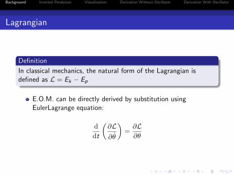
In classical mechanics, the natural form of the Lagrangian isdefined as L = Ek − Ep
E.O.M. can be directly derived by substitution usingEulerLagrange equation:
d
dt
(∂L∂θ
)=∂L∂θ
Background Inverted Pendulum Visualization Derivation Without Oscillator Derivation With Oscillator
Lagrangian
Definition
In classical mechanics, the natural form of the Lagrangian isdefined as L = Ek − Ep
E.O.M. can be directly derived by substitution usingEulerLagrange equation:
d
dt
(∂L∂θ
)=∂L∂θ
Background Inverted Pendulum Visualization Derivation Without Oscillator Derivation With Oscillator
Inverted Pendulum Problem
The pendulum is a stiff bar of length L which is supported atone end by a frictionless pin
The pin is given an oscillating vertical motion s defined by:
s(t) = A sinωt
Problem
Our problem is to derive the E.O.M. which relates time with theacceleration of the angle from the vertical position
Background Inverted Pendulum Visualization Derivation Without Oscillator Derivation With Oscillator
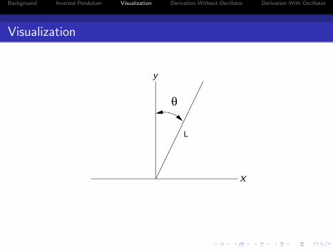
Visualization
Background Inverted Pendulum Visualization Derivation Without Oscillator Derivation With Oscillator
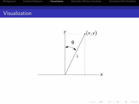
Visualization
Background Inverted Pendulum Visualization Derivation Without Oscillator Derivation With Oscillator
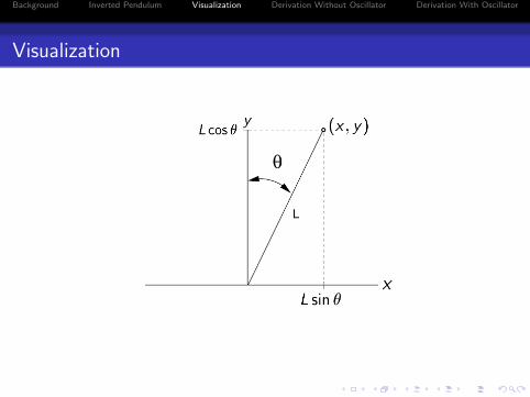
Visualization
Background Inverted Pendulum Visualization Derivation Without Oscillator Derivation With Oscillator
Visualization
Background Inverted Pendulum Visualization Derivation Without Oscillator Derivation With Oscillator
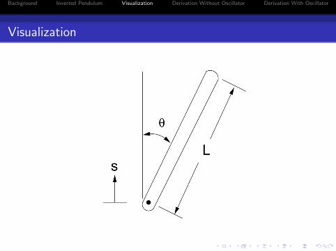
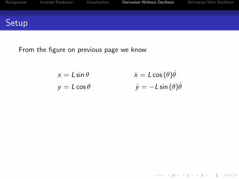
Setup
From the figure on previous page we know
x = L sin θ x = L cos (θ)θ
y = L cos θ y = −L sin (θ)θ
Recall the definition of the Lagrangian
L = Ek − Ep
L =1
2mv2 −mgy

Background Inverted Pendulum Visualization Derivation Without Oscillator Derivation With Oscillator
Setup
From the figure on previous page we know
x = L sin θ x = L cos (θ)θ
y = L cos θ y = −L sin (θ)θ
Recall the definition of the Lagrangian
L = Ek − Ep
L =1
2mv2 −mgy
Background Inverted Pendulum Visualization Derivation Without Oscillator Derivation With Oscillator
Setup Continued...
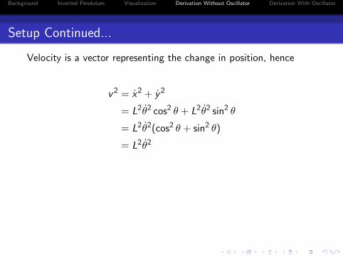
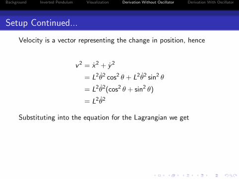
Velocity is a vector representing the change in position, hence
v2 = x2 + y2
= L2θ2 cos2 θ + L2θ2 sin2 θ
= L2θ2(cos2 θ + sin2 θ)
= L2θ2
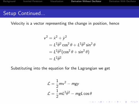
Substituting into the equation for the Lagrangian we get
L =1
2mv2 −mgy
L =1
2mL2θ2 −mgL cos θ
Background Inverted Pendulum Visualization Derivation Without Oscillator Derivation With Oscillator
Setup Continued...
Velocity is a vector representing the change in position, hence
v2 = x2 + y2
= L2θ2 cos2 θ + L2θ2 sin2 θ
= L2θ2(cos2 θ + sin2 θ)
= L2θ2
Substituting into the equation for the Lagrangian we get
L =1
2mv2 −mgy
L =1
2mL2θ2 −mgL cos θ
Background Inverted Pendulum Visualization Derivation Without Oscillator Derivation With Oscillator
Setup Continued...
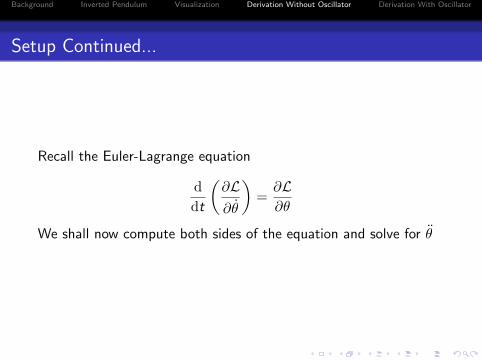
Recall the Euler-Lagrange equation
d
dt
(∂L∂θ
)=∂L∂θ
We shall now compute both sides of the equation and solve for θ
Background Inverted Pendulum Visualization Derivation Without Oscillator Derivation With Oscillator
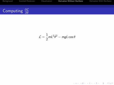
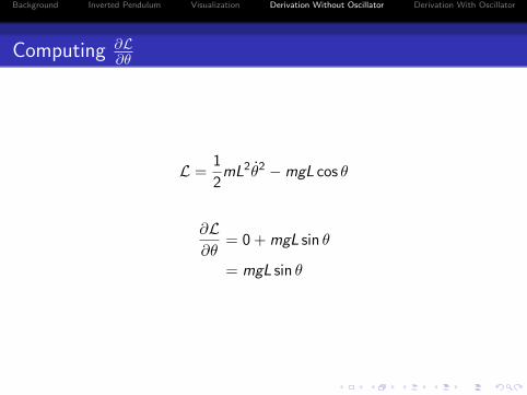
Computing ∂L∂θ
L =1
2mL2θ2 −mgL cos θ
∂L∂θ
= 0 + mgL sin θ
= mgL sin θ
Background Inverted Pendulum Visualization Derivation Without Oscillator Derivation With Oscillator
Computing ∂L∂θ
L =1
2mL2θ2 −mgL cos θ
∂L∂θ
= 0 + mgL sin θ
= mgL sin θ
Background Inverted Pendulum Visualization Derivation Without Oscillator Derivation With Oscillator
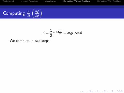
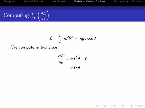
Computing ddt
(∂L∂θ
)
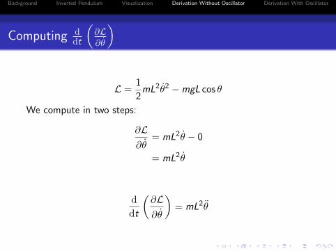
L =1
2mL2θ2 −mgL cos θ
We compute in two steps:
∂L∂θ
= mL2θ − 0
= mL2θ
d
dt
(∂L∂θ
)= mL2θ
Background Inverted Pendulum Visualization Derivation Without Oscillator Derivation With Oscillator
Computing ddt
(∂L∂θ
)
L =1
2mL2θ2 −mgL cos θ
We compute in two steps:
∂L∂θ
= mL2θ − 0
= mL2θ
d
dt
(∂L∂θ
)= mL2θ
Background Inverted Pendulum Visualization Derivation Without Oscillator Derivation With Oscillator
Computing ddt
(∂L∂θ
)
L =1
2mL2θ2 −mgL cos θ
We compute in two steps:
∂L∂θ
= mL2θ − 0
= mL2θ
d
dt
(∂L∂θ
)= mL2θ
Background Inverted Pendulum Visualization Derivation Without Oscillator Derivation With Oscillator
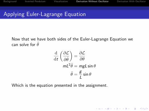
Applying Euler-Lagrange Equation
Now that we have both sides of the Euler-Lagrange Equation wecan solve for θ
d
dt
(∂L∂θ
)=∂L∂θ
mL2θ = mgL sin θ
θ =g
Lsin θ
Which is the equation presented in the assignment.
Background Inverted Pendulum Visualization Derivation Without Oscillator Derivation With Oscillator
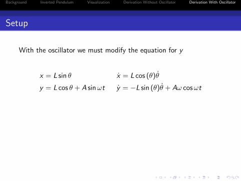
Setup
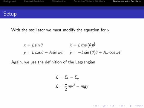
With the oscillator we must modify the equation for y
x = L sin θ x = L cos (θ)θ
y = L cos θ + A sinωt y = −L sin (θ)θ + Aω cosωt
Again, we use the definition of the Lagrangian
L = Ek − Ep
L =1
2mv2 −mgy
Background Inverted Pendulum Visualization Derivation Without Oscillator Derivation With Oscillator
Setup
With the oscillator we must modify the equation for y
x = L sin θ x = L cos (θ)θ
y = L cos θ + A sinωt y = −L sin (θ)θ + Aω cosωt
Again, we use the definition of the Lagrangian
L = Ek − Ep
L =1
2mv2 −mgy
Background Inverted Pendulum Visualization Derivation Without Oscillator Derivation With Oscillator
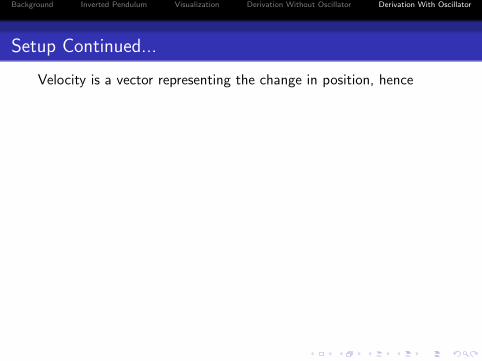
Setup Continued...
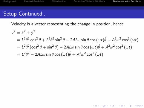
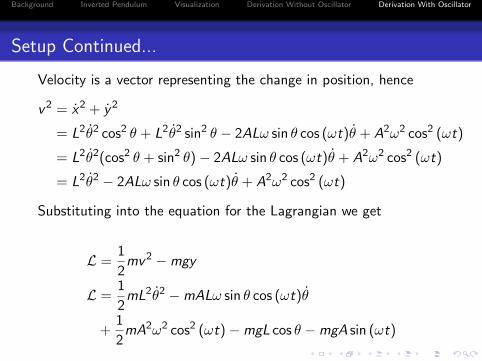
Velocity is a vector representing the change in position, hence
v2 = x2 + y2
= L2θ2 cos2 θ + L2θ2 sin2 θ − 2ALω sin θ cos (ωt)θ + A2ω2 cos2 (ωt)
= L2θ2(cos2 θ + sin2 θ)− 2ALω sin θ cos (ωt)θ + A2ω2 cos2 (ωt)
= L2θ2 − 2ALω sin θ cos (ωt)θ + A2ω2 cos2 (ωt)
Substituting into the equation for the Lagrangian we get
L =1
2mv2 −mgy
L =1
2mL2θ2 −mALω sin θ cos (ωt)θ
+1
2mA2ω2 cos2 (ωt)−mgL cos θ −mgA sin (ωt)
Background Inverted Pendulum Visualization Derivation Without Oscillator Derivation With Oscillator
Setup Continued...
Velocity is a vector representing the change in position, hence
v2 = x2 + y2
= L2θ2 cos2 θ + L2θ2 sin2 θ − 2ALω sin θ cos (ωt)θ + A2ω2 cos2 (ωt)
= L2θ2(cos2 θ + sin2 θ)− 2ALω sin θ cos (ωt)θ + A2ω2 cos2 (ωt)
= L2θ2 − 2ALω sin θ cos (ωt)θ + A2ω2 cos2 (ωt)
Substituting into the equation for the Lagrangian we get
L =1
2mv2 −mgy
L =1
2mL2θ2 −mALω sin θ cos (ωt)θ
+1
2mA2ω2 cos2 (ωt)−mgL cos θ −mgA sin (ωt)
Background Inverted Pendulum Visualization Derivation Without Oscillator Derivation With Oscillator
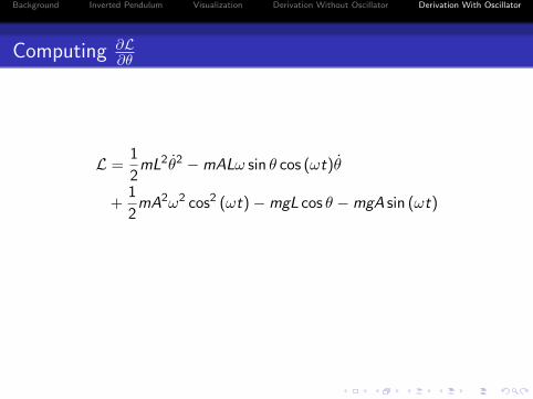
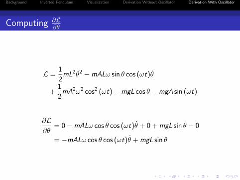
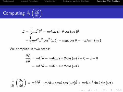
Computing ∂L∂θ
L =1
2mL2θ2 −mALω sin θ cos (ωt)θ
+1
2mA2ω2 cos2 (ωt)−mgL cos θ −mgA sin (ωt)
∂L∂θ
= 0−mALω cos θ cos (ωt)θ + 0 + mgL sin θ − 0
= −mALω cos θ cos (ωt)θ + mgL sin θ
Background Inverted Pendulum Visualization Derivation Without Oscillator Derivation With Oscillator
Computing ∂L∂θ
L =1
2mL2θ2 −mALω sin θ cos (ωt)θ
+1
2mA2ω2 cos2 (ωt)−mgL cos θ −mgA sin (ωt)
∂L∂θ
= 0−mALω cos θ cos (ωt)θ + 0 + mgL sin θ − 0
= −mALω cos θ cos (ωt)θ + mgL sin θ
Background Inverted Pendulum Visualization Derivation Without Oscillator Derivation With Oscillator
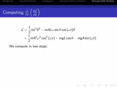
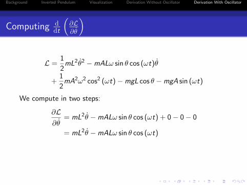
Computing ddt
(∂L∂θ
)
L =1
2mL2θ2 −mALω sin θ cos (ωt)θ
+1
2mA2ω2 cos2 (ωt)−mgL cos θ −mgA sin (ωt)
We compute in two steps:
∂L∂θ
= mL2θ −mALω sin θ cos (ωt) + 0− 0− 0
= mL2θ −mALω sin θ cos (ωt)
d
dt
(∂L∂θ
)= mL2θ −mALω cos θ cos (ωt)θ + mALω2 sin θ sin (ωt)
Background Inverted Pendulum Visualization Derivation Without Oscillator Derivation With Oscillator
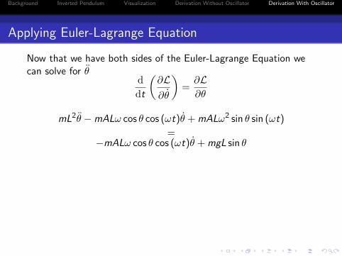
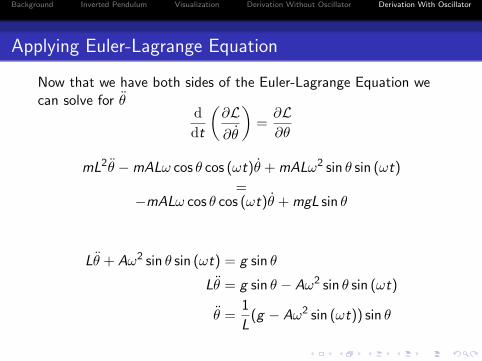
Applying Euler-Lagrange Equation
Now that we have both sides of the Euler-Lagrange Equation wecan solve for θ
d
dt
(∂L∂θ
)=∂L∂θ
mL2θ −mALω cos θ cos (ωt)θ + mALω2 sin θ sin (ωt)
=−mALω cos θ cos (ωt)θ + mgL sin θ
Lθ + Aω2 sin θ sin (ωt) = g sin θ
Lθ = g sin θ − Aω2 sin θ sin (ωt)
θ =1
L(g − Aω2 sin (ωt)) sin θ
Background Inverted Pendulum Visualization Derivation Without Oscillator Derivation With Oscillator
References
http://en.wikipedia.org/wiki/Euler-Lagrange equation
http://en.wikipedia.org/wiki/Lagrangian mechanics
http://en.wikipedia.org/wiki/Newton’s laws of motion