Derivative-driven window-based regression method for gas turbine performance prognostics

TSOUTSANIS, Elias <http://orcid.org/0000-0001-8476-4726> and MESKIN, Nader

Available from Sheffield Hallam University Research Archive (SHURA) at:

http://shura.shu.ac.uk/16175/

This document is the author deposited version. You are advised to consult the publisher's version if you wish to cite from it.

Published version

TSOUTSANIS, Elias and MESKIN, Nader (2017). Derivative-driven window-based regression method for gas turbine performance prognostics. Energy, 128, 302-311.

Copyright and re-use policy

See http://shura.shu.ac.uk/information.html

Sheffield Hallam University Research Archivehttp://shura.shu.ac.uk

brought to you by COREView metadata, citation and similar papers at core.ac.uk

provided by Sheffield Hallam University Research Archive

Derivative-driven window-based regression method for gas turbine

performance prognostics

Elias Tsoutsanisa,∗, Nader Meskinb

aSchool of Engineering, Emirates Aviation University, Dubai, United Arab EmiratesbDepartment of Electrical Engineering, College of Engineering, Qatar University, Doha, Qatar

Abstract

The domination of gas turbines in the energy arena is facing many challenges from environmental regulations

and the plethora of renewable energy sources. The gas turbine has to operate under demand-driven modes

and its components consume their useful life faster than the engines of the base-load operation era. As a

result the diagnostics and prognostics tools should be further developed to cope with the above operation

modes and improve the condition based maintenance (CBM).

In this study, we present a derivative-driven diagnostic pattern analysis method for estimating the per-

formance of gas turbines under dynamic conditions. A real time model-based tuner is implemented through

a dynamic engine model built in Matlab/Simulink for diagnostics. The nonlinear diagnostic pattern is then

partitioned into data-windows. These are the outcome of a data analysis based on the second order deriva-

tive which corresponds to the acceleration of degradation. Linear regression is implemented to locally fit

the detected deviations and predict the engine behavior. The accuracy of the proposed method is assessed

through comparison between the predicted and actual degradation by the remaining useful life (RUL) metric.

The results demonstrate and illustrate an improved accuracy of our proposed methodology for prognostics

of gas turbines under dynamic modes.

Keywords: Derivative-Driven Analysis, Window-Based Regression, Gas Turbine Prognostics, Condition

Based Maintenance

Highlights

• A data-based method for gas turbine performance prognostics is developed.

• The proposed method takes into account dynamic operating modes and employs a derivative-driven

diagnostic pattern analysis.

• Linear regression is performed on a local data window manner to detect degradation.

∗Corresponding authorEmail address: elias.tsoutsanis@emirates.com (Elias Tsoutsanis)

Preprint submitted to Energy March 21, 2017

• The accuracy of the method is tested under transient operating conditions and compared to an earlier

method.

• The proposed method is capable of detecting accurately the evolution of compressor fouling.

Nomenclature

Symbols

A acceleration of component performance degradation ∆X

g1−2 coefficients of linear regression

k acceleration threshold

L width of window

m mass flow rate

n total number of operating points

N corrected shaft rotational speed

P total pressure

q total number of windows

T total temperature

u ambient and operating conditions vector

W useful power output

x component performance parameter

X component characteristics vector

Y measurement vector

Greek

Γ mass flow capacity

ǫ prediction error

∆ deviation

η isentropic efficiency

π pressure ratio

σ spread

Subscript

c compressor

d degraded

exh exhaust

2

f fuel

lreg linear regression

pt power turbine

r reference engine

t turbine

th thermal

1− 6 engine gas path location

1. Introduction1

The continuously growing energy demand along with the challenging aspect of reducing greenhouse2

emissions has transformed the power generation sector. Nowadays, the conventional fossil-fuelled power3

plants are required to work in partnership with the intermittent renewable energy plants for maintaining4

the stability and reliability of the electricity grid. This has reformed the gas turbine powered plants. The5

gas turbines are currently required to start up and shut down faster for satisfying the energy demand that6

fluctuates according to the intermittent character of the renewables energy sources. An emerging group of7

works in the literature has addressed the challenging aspect of the part-load performance behavior of gas8

turbines both at steady state [1, 2] and dynamic/transient conditions [3, 4, 5, 6] for optimizing the energy9

production and the stability of the electricity grid [7, 8].10

Under such dynamic conditions and grid-following modes both the renewable and gas turbine subsystems11

are expected to degrade at different rates [9, 10] and more importantly to consume their useful life faster12

than that of a system operating at base-load conditions. Therefore, the CBM of gas turbine systems is going13

to be affected by this recent shift in the engine operating profile.14

By principle, the diagnostic and prognostic tools [11, 12, 13, 14, 15] not only improve our understanding15

for complex and nonlinear systems such as the gas turbines but their accuracy and reliability are transferable16

to the effectiveness of the CBM. An example of the impact that these decision making tools have in the CBM17

can be found in the latest GE Digital Twin and Predix technologies [16]. It follows that the gas turbine18

community is faced with the challenging aspect of improving the accuracy of diagnostics and especially19

prognostics solutions for engines operating under dynamic conditions. Apart from a limited number of20

works available in the literature [17, 18, 19, 20, 21], the majority of the existing diagnostic methods are21

based on steady state operation. Subsequently, the majority of the existing prognostics methods have been22

developed and tested by taking into consideration diagnostic information that was primarily based on the23

steady state conditions .24

The ever growing development of prognostic schemes for gas turbine engines has resulted into a large25

number of prognostic solutions. Generally, these schemes can be divided into two categories, such as data-26

3

based and model-based approaches. Amongst the data-based prognostic methods the most popular are27

neural networks [22, 23] and bayesian networks [24, 25]. A subgroup of the data-based methods are the28

statistical approaches [26, 27] in which their primary focus is that of forecasting the behavior of a system29

without necessarily evaluating the remaining useful life of the component.30

Model-based methods rely heavily on engine model diagnosis which is directly coupled to the prognosis31

process. For the model-based approaches the most commonly used method is that of trending the available32

diagnostic information through linear and nonlinear regression models [28, 29]. Another popular model-33

based prognostic solution is based on the particle filtering [30, 31, 32, 33, 34] methods. Finally, there is a34

family of hybrid prognostic approaches [35, 10] that combine algorithms coming from the model-based and35

data-based groups. From the numerous methods employed for gas turbine prognostics only a few examples36

in the literature [28, 10] have employed dynamic/transient operational modes for diagnosis [18, 32, 36] and37

prognosis.38

Therefore, the development of a prognostic system capable of taking into account the dynamic gas39

turbine operation is fundamental for an effective and successful CBM. Dynamic operating gas turbines have40

to be monitored at an increased frequency rate which results in a vast amount of data for the gas turbine41

operators to process, analyze and interpret towards to facilitating the maintenance and operation of the42

engines. In addition, the fast and highly nonlinear engine dynamics make the interpretation of the gas path43

information a very complex task since it moves away from the common practice of the industry to forecast44

the behavior of the engine based on its entire operational history. It would be more practical to focus the45

prognostic analysis for such dynamic gas turbines in the short-term since the electricity demand dominated46

by the intermittent character of the renewables affects the operating profile of the gas turbines and alters47

significantly the degradation pattern of its components. Within this context and taking into consideration48

the vast amount of engine monitored information contained in data lakes the aim of this study is to develop49

a method for accurately forecasting the engine component degradation into the future by examining the50

rate by which the degradation changes with respect to time.51

Generally, the gas turbine engine performance depends on its components behavior. In our recent52

study [37], an advanced model-based adaptation method was combined with a dynamic gas turbine model53

developed in Matlab/Simulink. The outcome of this process was a uniquely tuned set of engine component54

maps that empowered the engine model to match the performance measurements of a reference engine55

operating under transient diagnostics.56

From our recent work [10] on prognostics we utilized an adaptive diagnostic process [18] for a number of57

sliding windows capturing the entire degraded measurements. Subsequently, the detected degradation was58

used for a linear regression towards prognostics. In contrast to our earlier study, the proposed method em-59

ploys a real time data-driven tuner that performs the diagnosis online and each operating point corresponds60

to a different set of component maps. The information containing the diagnostic data is then divided into61

4

smaller time segments referred to as windows. The time range of each window, referred to as width, depends62

on the time data series distribution. Specifically, the data distribution examined refers to the acceleration63

of degradation which is represented as the second order derivative of the predicted deviations. It follows,64

that the bank of data encapsulated in the collection of windows are utilized in a local linear window-based65

manner for predicting the future behavior of the engine components. The current work is an extension of66

our recent work [38] which includes a comparison of the proposed method with the one presented in [10].67

The accuracy improvement of the proposed method is tested for evaluating the level of compressor fouling68

when the engine experiences concurrently multiple component degradations. At the same time the engine69

operates under dynamic/transient conditions for a period of time that corresponds to 25,000 h. The metrics70

of RUL and the PDF [39, 40, 41] have been utilized to assess and evaluate the accuracy improvement of71

the proposed method over the one developed earlier by the authors [10]. Finally, this prognostic tool can72

facilitate the gas turbine operators to increase their awareness for the performance of their gas turbine assets73

when these operate under transient conditions and enable them to optimize the operation of their plants.74

To summarize the main contributions of this paper can be listed as follows:75

1. The problem of fault prognosis of an industrial gas turbine under transient conditions is investigated by76

using a regression method which is activated by a derivative-driven criterion of detected degradations.77

2. Compared to the previous related works, the proposed method represents a powerful tool for forecast-78

ing the evolution of degraded component performance without taking into account the entire diagnostic79

history of the equipment. This is achieved by splitting the detected component degradation pattern80

into smaller increments where the evolutions of degradation can be assumed to be linear with respect81

to time.82

3. Moreover, the distribution of diagnostic data is examined based on a second order derivative crite-83

rion which corresponds to the acceleration of degradation. Upon this criterion the diagnostic pattern84

is partitioned into smaller segments that we refer to as windows and the contained information is85

implemented for performing short-term prognostics. This is the first time in the literature that the86

acceleration of the diagnostic data is utilized for simplifying the prognostic process.87

4. Furthermore, we compare the proposed method with the one developed earlier by the authors [10] in88

order to demonstrate and illustrate the prediction accuracy improvement through the use of PDF and89

RUL metrics.90

5. The main benefit of the proposed prognostic method is its ability to simplify the nonlinear time evolving91

component degradation into a simple local and linear process for which meaningful prognostic results92

can be easily interpreted. Using the proposed technique, the prognosis is generalized for gas turbine93

dynamic operating modes and can be further employed for other demand-driven energy equipment.94

5

The remainder of this paper is organized as follows. In Section 2, the proposed prognostic method along95

with the concept of performance adaptation used for diagnostics and its integration with a dynamic engine96

model are described. The description of the case studies are presented in Section 3. Simulation results of97

the proposed approach are presented in Section 4, followed by the conclusions in Section 5.98

2. Methodology99

2.1. Assumptions100

The component performance degradation of gas turbines is mainly attributed to the ambient conditions,101

the operating mode and the manufacturing tolerances. These factors increase the complexity of the diagnos-102

tics and subsequently the prognostics tasks. This is evident by the numerous existing prognostic solutions103

proposed for gas turbines. In this study several assumptions have been made, for facilitating the application104

of the proposed method to service engines, as follows:105

• Only incipient component performance faults (no abrupt) are considered for prognostics.106

• All the engine components are experiencing performance degradations simultaneously.107

• The performance degradation of each component corresponds to deviations of the mass flow capacity108

and isentropic efficiency from their clean/healthy values.109

• The pattern of degradations examined are monotonical.110

• The operating conditions are varying with respect to time.111

The above assumptions rely on the fact that modern gas turbine that operate under dynamic conditions112

maintain a monotonically pattern of degradation even if regular maintenance actions such as online and/or113

offline compressor washings are performed. As far as the gas path information provided by the instrumen-114

tation set we assume that there is no presence of noise and bias. The reason for this lies in the fact that115

the main aim of this study is to focus purely on the capability of the developed method to deal effectively116

with the estimation of the component degradation pattern and not on the validity of the sensor informa-117

tion. Other approaches for data-smoothing and noise-filtering could be performed prior to diagnostics and118

prognostics for ensuring a good quality data set for the above purposes.119

2.2. Model Tuning120

The frequently performed maintenance actions in industrial gas turbines (such as online/offline compres-121

sor washing, replacement of inlet filtration systems, fuel nozzles and sensors) and the evolving performance122

degradation of their components alter the performance and health signature of the engine. Therefore, gas123

turbine users have to progressively refine and update their engine models for improving the accuracy of124

6

the performance prediction based on available service engine data. This process is commonly referred to as125

model-based performance adaptation and deals with the optimization of component-based parameters such126

as mass flow capacities and efficiencies so that the service engine measurable performance parameters such127

as gas path temperatures and pressures are properly matched. This is a minimization problem since its goal128

is to mimimize the observed residuals between the model predictions and the engine test data. This process129

establishes the data-set that corresponds to the healthy engine condition. It follows that data from a family130

of adapted engine models can be implemented for performance-based diagnostic analysis.131

Model

Map Th/cs

Reference Engine

OF

Min?Stop

Yes

No

u

X Y

Yr

Map Tuning

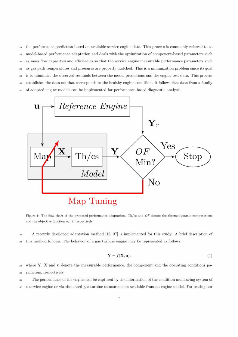
Figure 1: The flow chart of the proposed performance adaptation. Th/cs and OF denote the thermodynamic computations

and the objective function eq. 2, respectively.

A recently developed adaptation method [18, 37] is implemented for this study. A brief description of132

this method follows. The behavior of a gas turbine engine may be represented as follows:133

Y = f(X,u), (1)

where Y, X and u denote the measurable performance, the component and the operating conditions pa-134

rameters, respectively.135

The performance of the engine can be captured by the information of the condition monitoring system of136

a service engine or via simulated gas turbine measurements available from an engine model. For testing our137

7

proposed method two gas turbine models are used. The gas turbine model that implements the component138

characteristics of PROOSIS [42] simulation software is referred to as the reference engine and acts as the test139

engine in this study. The second model, which is going to be referred to as the engine model, implements140

the recently developed adaptation concept [37].141

The deviations between the engine model predictions Y and the reference engine observations Yr are142

evaluated by the Objective Function (OF ) as follows:143

OF =

√

√

√

√

n∑

i=1

(

Yi −Yri

Yri

)2

, (2)

where n denotes the number of the operating points and Yi and Yri denote the i-th predicted and observable144

performance parameter, respectively.145

For initial engine model adaptation the data generated by the reference engine are matched by the engine146

model on a global scale i.e. a single set of component maps is progressively tuned in order minimize the147

observed residuals. For a more detailed description and analysis of the adaptation concept the reader is148

prompted to our earlier works [18, 37].149

Degraded Reference Engine

5 10 15 20 25 30 35

5

10

Corrected Mass Flow Rate, mc

Pressure

Ratio,πc

Component map

5,000 10,000 15,000 20,000 25,000−4

−3

−2

−1

0

Time (h)

Injected

deviation

incompressor

efficien

cy(%

)

Injected degradation

Thermodynamic

Computations

u

t

Xr

∆Xrinj

XrdYrd

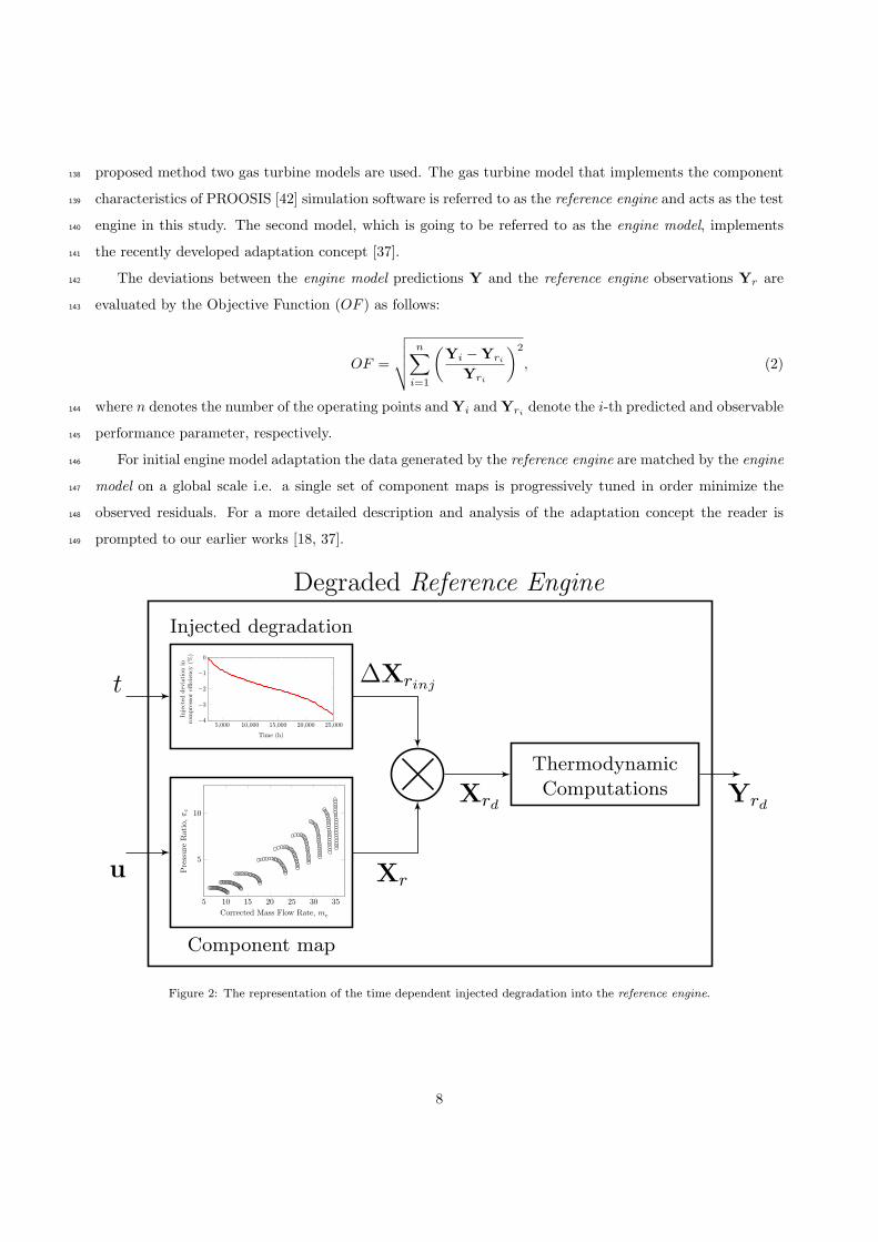
Figure 2: The representation of the time dependent injected degradation into the reference engine.

8

2.3. Diagnostics150

Generally the performance deterioration of engine components is oftenly represented by the component151

parameter deviation ∆X from its nominal/clean value and given by:152

∆X = 100× (Xd −X) /X. (3)

where X and Xd denote the clean and degraded component parameter, respectively.153

For representing the time evolving performance degradation, the component maps of the reference engine154

are injected with deviation signals which alter the mass flow capacity and efficiency outputs of each com-155

ponent. Consequently, the initial healthy parameter of the reference engine Xr is deviated by the injected156

signal ∆Xrinjresulting in a fault-contaminated component map output Xrd . This in turn is reflected in the157

measurable parameter Yrd of the reference engine which corresponds to degraded conditions, as seen from158

Fig. 2.159

The component degradation ∆Xrinjwith respect to time t may be represented as a function g, i.e.160

∆Xrinj(t) = g(t). The mathematical form of the function g depends on the injected deviation signal. In161

practise, the evolution of component degradation can be captured by a variety of functions however the162

most common approach is data-trending through linear and polynomial regression models.163

At this stage the objective of the diagnosis task deals with estimating the level of the component degra-164

dation of the reference engine. The performance adaptation is once again implemented for performing the165

diagnostic task. However, there is a major difference in the way that the adaptation is implemented here166

for the diagnostic purpose. The initial adapted component maps remain unaffected and only their output,167

as shown in Fig. 3, is further tuned. This process can be performed real time by employing the algebraic168

constraint function of Matlab/Simulink. In contrary to our earlier works, where the adaptation concept169

was implemented for diagnostics on a global scale, this approach is performed locally for every operating170

point and the corresponding generated component maps are utilized for matching the evolving degraded171

measurements.172

The accuracy of the diagnostic task is evaluated by the Diagnostic Index (DI) [37] as follows:173

DI = 100

(

1

1 + ǫ

)

, (4)

where ǫ is the detected residual for the component parameter X as follows:174

ǫ =

n∑

i=1

∣

∣

∣

∣

∆Xi−∆Xrinji

∆Xrinji

∣

∣

∣

∣

n. (5)

At this point it should be pointed out that the accuracy of the diagnostic and subsequently the prog-175

nostic processes is relying heavily on the capability of the engine model to adapt its component parameters176

9

Model

Map

Th/cs

Reference Engine

OF

Min?Stop

Yes

No

u

X

Xd Yd

Yrd

Adaptive Diagnosis

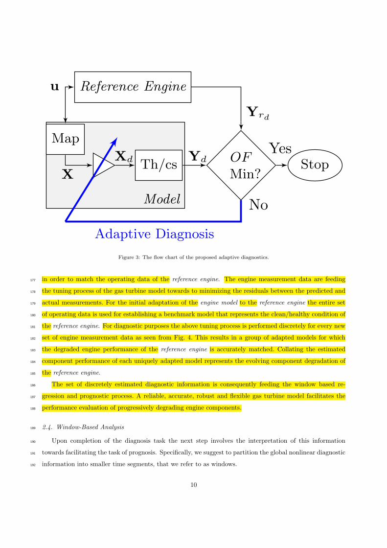
Figure 3: The flow chart of the proposed adaptive diagnostics.

in order to match the operating data of the reference engine. The engine measurement data are feeding177

the tuning process of the gas turbine model towards to minimizing the residuals between the predicted and178

actual measurements. For the initial adaptation of the engine model to the reference engine the entire set179

of operating data is used for establishing a benchmark model that represents the clean/healthy condition of180

the reference engine. For diagnostic purposes the above tuning process is performed discretely for every new181

set of engine measurement data as seen from Fig. 4. This results in a group of adapted models for which182

the degraded engine performance of the reference engine is accurately matched. Collating the estimated183

component performance of each uniquely adapted model represents the evolving component degradation of184

the reference engine.185

The set of discretely estimated diagnostic information is consequently feeding the window based re-186

gression and prognostic process. A reliable, accurate, robust and flexible gas turbine model facilitates the187

performance evaluation of progressively degrading engine components.188

2.4. Window-Based Analysis189

Upon completion of the diagnosis task the next step involves the interpretation of this information190

towards facilitating the task of prognosis. Specifically, we suggest to partition the global nonlinear diagnostic191

information into smaller time segments, that we refer to as windows.192

10

Model

Map Th/cs

Reference Engine

OF

Min?Stop

Yes

No

u

X Y

Yr

Map Tuning

Model

Map

Th/cs

Reference Engine

OF

Min?Stop

Yes

No

u

X

Xd Yd

Yrd

Adaptive Diagnosis

Model

Map

Th/cs

Reference Engine

OF

Min?Stop

Yes

No

u

X

Xd Yd

Yrd

Adaptive Diagnosis

Model

Map

Th/cs

Reference Engine

OF

Min?Stop

Yes

No

u

X

Xd Yd

Yrd

Adaptive Diagnosis

Model

Map

Th/cs

Reference Engine

OF

Min?Stop

Yes

No

u

X

Xd Yd

Yrd

Adaptive Diagnosis

Initial AdaptationGlobal

Model A

DiagnosticsLocal

Model D1

Model D2

Model D3

...Model Dn

Yr

Time

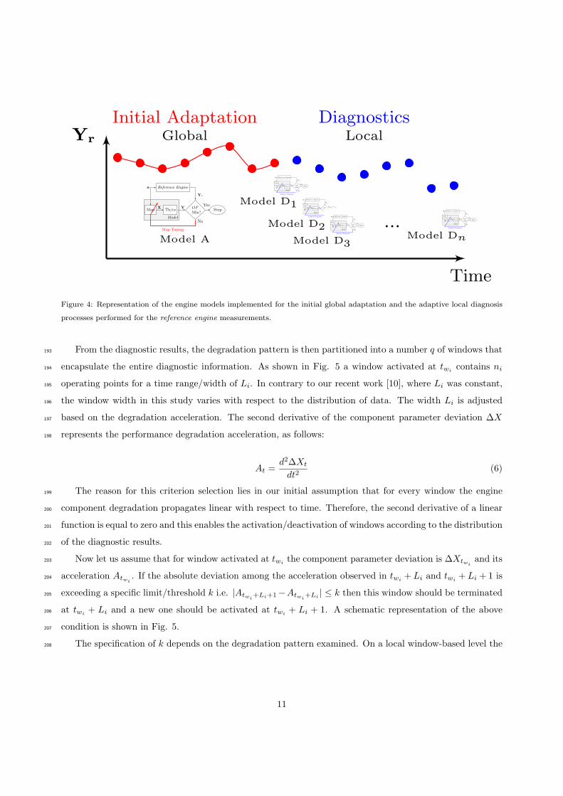
Figure 4: Representation of the engine models implemented for the initial global adaptation and the adaptive local diagnosis

processes performed for the reference engine measurements.

From the diagnostic results, the degradation pattern is then partitioned into a number q of windows that193

encapsulate the entire diagnostic information. As shown in Fig. 5 a window activated at twicontains ni194

operating points for a time range/width of Li. In contrary to our recent work [10], where Li was constant,195

the window width in this study varies with respect to the distribution of data. The width Li is adjusted196

based on the degradation acceleration. The second derivative of the component parameter deviation ∆X197

represents the performance degradation acceleration, as follows:198

At =d2∆Xt

dt2(6)

The reason for this criterion selection lies in our initial assumption that for every window the engine199

component degradation propagates linear with respect to time. Therefore, the second derivative of a linear200

function is equal to zero and this enables the activation/deactivation of windows according to the distribution201

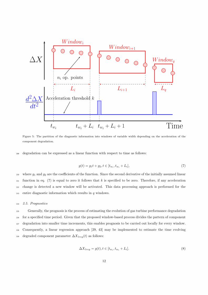
of the diagnostic results.202

Now let us assume that for window activated at twithe component parameter deviation is ∆Xtwi

and its203

acceleration Atwi. If the absolute deviation among the acceleration observed in twi

+Li and twi+Li + 1 is204

exceeding a specific limit/threshold k i.e. |Atwi+Li+1−Atwi

+Li| ≤ k then this window should be terminated205

at twi+ Li and a new one should be activated at twi

+ Li + 1. A schematic representation of the above206

condition is shown in Fig. 5.207

The specification of k depends on the degradation pattern examined. On a local window-based level the208

11

∆X

d2∆Xdt2

Time

ni op. points

Acceleration threshold k

Windowi

Li

Windowi+1

Li+1

Windowq

Lq

twi twi+ Li twi

+ Li + 1

Figure 5: The partition of the diagnostic information into windows of variable width depending on the acceleration of the

component degradation.

degradation can be expressed as a linear function with respect to time as follows:209

g(t) = g1t+ g2, t ∈ [twi, twi

+ Li], (7)

where g1 and g2 are the coefficients of the function. Since the second derivative of the initially assumed linear210

function in eq. (7) is equal to zero it follows that k is specified to be zero. Therefore, if any acceleration211

change is detected a new window will be activated. This data processing approach is performed for the212

entire diagnostic information which results in q windows.213

2.5. Prognostics214

Generally, the prognosis is the process of estimating the evolution of gas turbine performance degradation215

for a specified time period. Given that the proposed window-based process divides the pattern of component216

degradation into smaller time increments, this enables prognosis to be carried out locally for every window.217

Consequently, a linear regression approach [29, 43] may be implemented to estimate the time evolving218

degraded component parameter ∆X lreg(t) as follows:219

∆X lreg = g(t), t ∈ [twi, twi

+ Li]. (8)

12

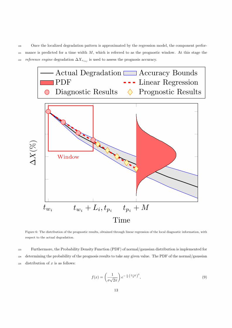
Once the localized degradation pattern is approximated by the regression model, the component perfor-220

mance is predicted for a time width M , which is referred to as the prognostic window. At this stage the221

reference engine degradation ∆Xrinjis used to assess the prognosis accuracy.222

twi twi+ Li, tpi

tpi+M

Window

Time

∆X(%

)

Actual Degradation Accuracy BoundsPDF Linear RegressionDiagnostic Results Prognostic Results

Figure 6: The distribution of the prognostic results, obtained through linear regression of the local diagnostic information, with

respect to the actual degradation.

Furthermore, the Probability Density Function (PDF) of normal/gaussian distribution is implemented for223

determining the probability of the prognosis results to take any given value. The PDF of the normal/gaussian224

distribution of x is as follows:225

f(x) =

(

1

σ√2π

)

e−1

2 (x−µσ )

2

, (9)

13

where x denotes the degraded component parameter ∆X lreg of standard deviation σ.226

The PDF of the linearly regressed component parameter ∆X lreg information along with the diagnostic227

predictions ∆X and the actual degradation ∆Xrinjwith its corresponding accuracy bounds is shown in Fig.228

6. The final step of the prognosis task is RUL estimation for the component.229

The majority of the performance-based prognostic algorithms for rotating machinery [29, 28] evaluate230

RUL by projecting the diagnostic predictions into time and assigning a probability of these predictions to231

reach a certain threshold. The proposed prognosis is adopting another logic since its main focus is the inves-232

tigation of the degradation pattern itself and how it evolves over time. The localized linear window-based233

analysis facilitates the short-term performance prediction of degraded components and the Equivalent RUL234

(ERUL) metric suggested by the authors is implemented for determining the evolution of the degradation235

in short-term intervals.236

Finally, accuracy bounds similar to the diagnostic accuracy bounds are implemented for the true ERUL.237

The true ERUL is determined by the injected degradation to the engine component parameters ∆Xrinj. As238

a result the comparison between estimated ERUL and true ERUL provides an insight to the performance239

capability of the proposed method. The ERUL represents the rate at which the component of the engine240

system ‘consumes’ its useful life according to the mode of operation.241

3. Case Study Description242

The proposed adaptive and window-based methods for prognostics approaches are integrated into a an243

industrial gas turbine model that is developed in MATLAB/Simulink environment. It is worth mentioning244

that the MATLAB/Simulink environment is becoming very popular for the analysis of energy systems245

dynamics and the design of controllers [44, 45, 46, 47]. Our developed model has been validated towards246

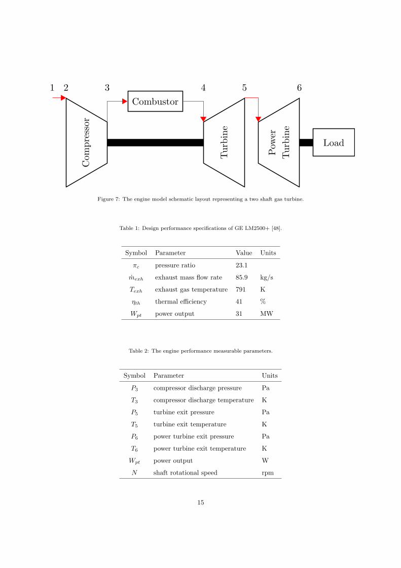
PROOSIS [42] simulation software. The engine model is similar to the GE LM2500+ aero derivative gas tur-247

bine [48] which is a two-shaft industrial gas turbine that consists of a compressor, a combustor, a compressor248

turbine and a power turbine as schematically represented in Fig 7. The design performance specifications of249

the engine are tabulated in Table 1.250

The control input of the gas turbine model configuration is the fuel flow rate mf . A detailed description251

of the gas turbine model can be found in our recent works in [49, 37]. The objective of the case studies252

is to evaluate the accuracy improvement of our prognostic method in comparison to the earlier prognostic253

scheme developed where fixed width windows were implemented. The selected measurable parameters for254

the diagnostic and prognostic tasks are listed in Table 2.255

Now let us describe the reference engine data generation process. The time step of the simulation256

procedure is 1 ms. For 100 s simulation time a total of 100,000 data samples are generated. The above data257

should be mapped to the examined component degradations that are typical for 25,000 h of operation. This258

14

1 2 3 4 5 6Com

pressor

Combustor

Turbine

Pow

er

Turbine

Load

Figure 7: The engine model schematic layout representing a two shaft gas turbine.

Table 1: Design performance specifications of GE LM2500+ [48].

Symbol Parameter Value Units

πc pressure ratio 23.1

mexh exhaust mass flow rate 85.9 kg/s

Texh exhaust gas temperature 791 K

ηth thermal efficiency 41 %

Wpt power output 31 MW

Table 2: The engine performance measurable parameters.

Symbol Parameter Units

P3 compressor discharge pressure Pa

T3 compressor discharge temperature K

P5 turbine exit pressure Pa

T5 turbine exit temperature K

P6 power turbine exit pressure Pa

T6 power turbine exit temperature K

Wpt power output W

N shaft rotational speed rpm

15

0 5, 000 10, 000 15, 000 20, 000 25, 0000.65

0.9

1.15

Time (h)

Fuel

flow

rate

mf/m

fdes

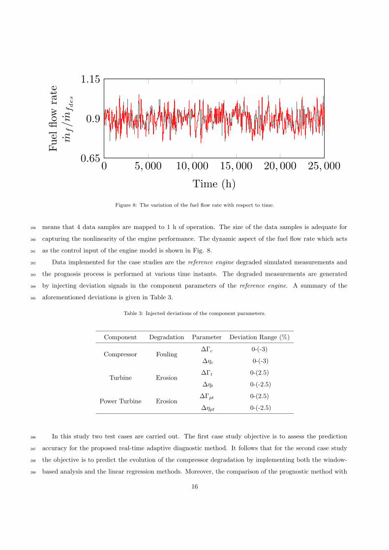
Figure 8: The variation of the fuel flow rate with respect to time.

means that 4 data samples are mapped to 1 h of operation. The size of the data samples is adequate for259

capturing the nonlinearity of the engine performance. The dynamic aspect of the fuel flow rate which acts260

as the control input of the engine model is shown in Fig. 8.261

Data implemented for the case studies are the reference engine degraded simulated measurements and262

the prognosis process is performed at various time instants. The degraded measurements are generated263

by injecting deviation signals in the component parameters of the reference engine. A summary of the264

aforementioned deviations is given in Table 3.265

Table 3: Injected deviations of the component parameters.

Component Degradation Parameter Deviation Range (%)

Compressor Fouling∆Γc

∆ηc

0-(-3)

0-(-3)

Turbine Erosion∆Γt

∆ηt

0-(2.5)

0-(-2.5)

Power Turbine Erosion∆Γpt

∆ηpt

0-(2.5)

0-(-2.5)

In this study two test cases are carried out. The first case study objective is to assess the prediction266

accuracy for the proposed real-time adaptive diagnostic method. It follows that for the second case study267

the objective is to predict the evolution of the compressor degradation by implementing both the window-268

based analysis and the linear regression methods. Moreover, the comparison of the prognostic method with269

16

the one earlier developed by the authors will give an insight of the accuracy improvement by the variable270

window-width activation introduced. Towards this end the common metrics of PDF and ERUL are utilized271

for assessing the accuracy of the prognosis.272

It should be noted that the earlier prognostic method will implement the diagnostic results on a different273

manner than in [10]. In the earlier study [10] the fixed width method was employed for both the diagnostic274

and prognostic process. The diagnosis in that case was carried out in a sliding window-based manner and275

for each diagnostic window the suite of engine model component maps were optimized and degradations276

were detected on a local window level. Consequently, the diagnostic information was the outcome of collated277

data from the detected degradations of each window. That approach had the advantage of partly filtering278

out the time component from the degradation so that the prognosis could be performed on a linear fixed-279

width window-based method. In contrast to our earlier work, this study waives off the added advantage of280

performing diagnosis in a window based fashion and only prognosis is performed on local window level.281

4. Results282

4.1. Diagnosis283

The model-based performance adaptation and the adaptive diagnostic method, are implemented for284

detecting the degradation of each component. The process commenced by initially adapting the engine285

model to the clean/nominal condition of reference engine for an operational profile that included both286

steady state and transient operating points. Then degradations were injected to the compressor, turbine287

and power turbine at td=2,500 h. The first bank of data up to td is utilized for engine model adaptation288

and denote the clean/nominal/healthy condition of the engine.289

Diagnostic tasks are initiated at td and carried out real time by tuning the output of each component290

map that has been initially optimized by the earlier adaptation process. The detected compressor fouling291

which is represented by the deviated mass flow component parameter is shown in Fig. 9. The diagnostic292

results indicated an improved accuracy in the diagnosis and in case of the compressor mass flow capacity293

the DI is 0.99 which implies that the diagnosis is 99% effective. It should be noted that all the compo-294

nent degradations have been detected with the same level of accuracy, but only the results concerning the295

compressor degradation are presented here.296

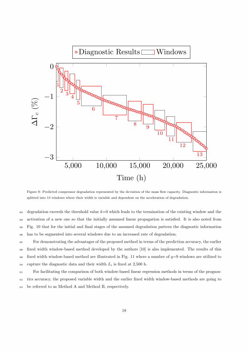
Prior to performing prognostics, the diagnostic information encapsulated by the detected deviations is297

split into a number of windows as seen from Fig. 9. For this case their time width Li relies solely on the298

distribution of the component degradation acceleration. The outcome of the above process resulted in a set299

of q=13 windows of variable width Li spanning from 250 h to 5,000 h.300

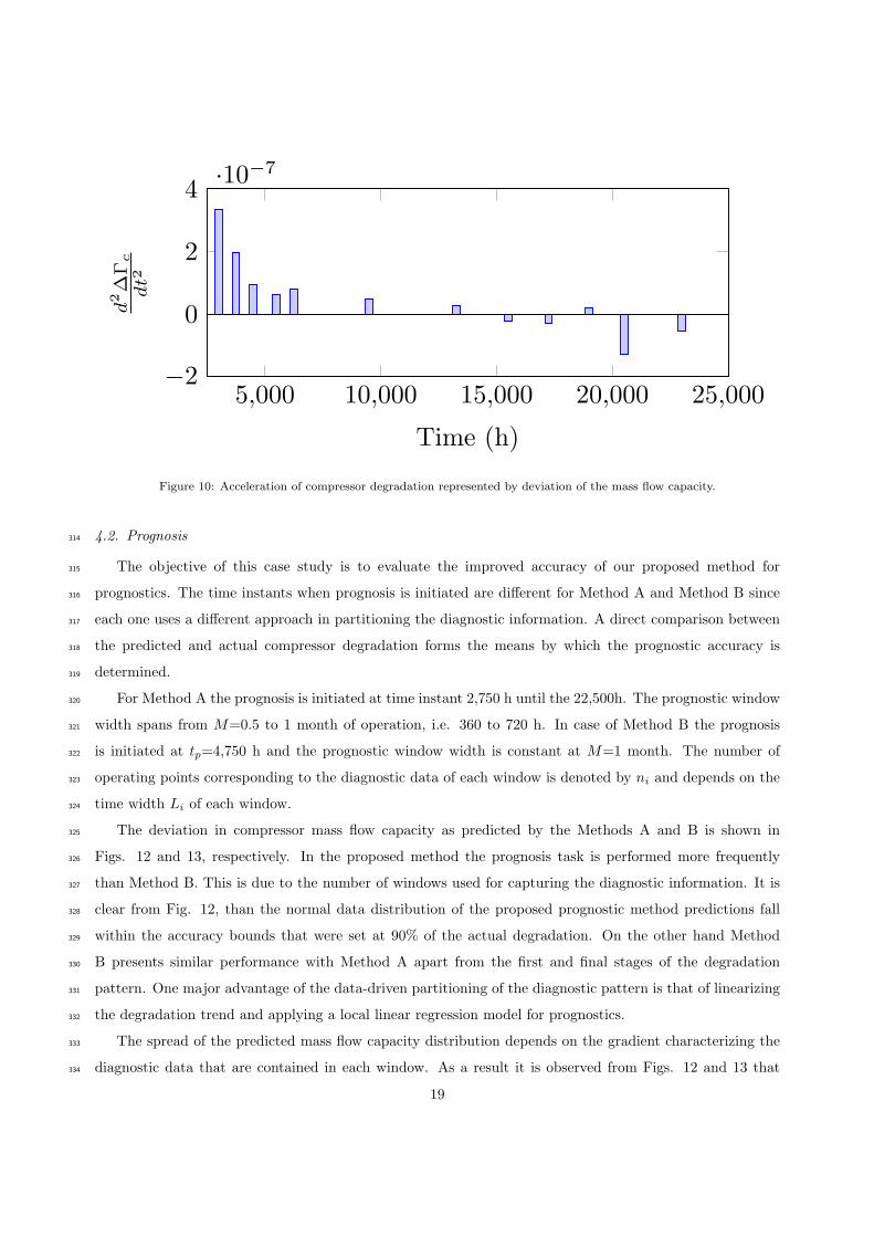
The acceleration of compressor degradation is represented by the second derivative of mass flow capac-301

ity with respect to time as seen from Fig. 10. At specific time instants, the acceleration of compressor302

17

5,000 10,000 15,000 20,000 25,000−3

−2

−1

0

1

23

4

5

6

7

89

10

11

12

13

Time (h)

∆Γc(%

)

Diagnostic Results Windows

Figure 9: Predicted compressor degradation represented by the deviation of the mass flow capacity. Diagnostic information is

splitted into 13 windows where their width is variable and dependent on the acceleration of degradation.

degradation exceeds the threshold value k=0 which leads to the termination of the existing window and the303

activation of a new one so that the initially assumed linear propagation is satisfied. It is also noted from304

Fig. 10 that for the initial and final stages of the assumed degradation pattern the diagnostic information305

has to be segmented into several windows due to an increased rate of degradation.306

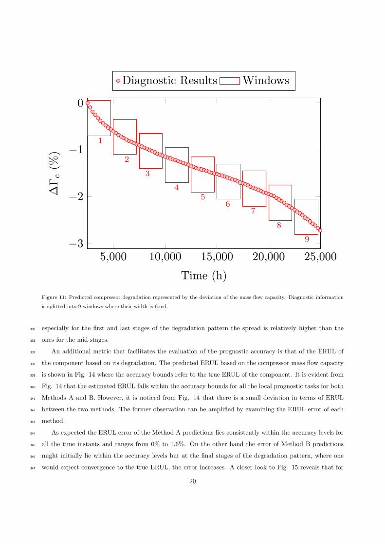
For demonstrating the advantages of the proposed method in terms of the prediction accuracy, the earlier307

fixed width window-based method developed by the authors [10] is also implemented. The results of this308

fixed width window-based method are illustrated in Fig. 11 where a number of q=9 windows are utilized to309

capture the diagnostic data and their width Li is fixed at 2,500 h.310

For facilitating the comparison of both window-based linear regression methods in terms of the prognos-311

tics accuracy, the proposed variable width and the earlier fixed width window-based methods are going to312

be referred to as Method A and Method B, respectively.313

18

5,000 10,000 15,000 20,000 25,000−2

0

2

4·10−7

Time (h)

d2∆Γc

dt2

Figure 10: Acceleration of compressor degradation represented by deviation of the mass flow capacity.

4.2. Prognosis314

The objective of this case study is to evaluate the improved accuracy of our proposed method for315

prognostics. The time instants when prognosis is initiated are different for Method A and Method B since316

each one uses a different approach in partitioning the diagnostic information. A direct comparison between317

the predicted and actual compressor degradation forms the means by which the prognostic accuracy is318

determined.319

For Method A the prognosis is initiated at time instant 2,750 h until the 22,500h. The prognostic window320

width spans from M=0.5 to 1 month of operation, i.e. 360 to 720 h. In case of Method B the prognosis321

is initiated at tp=4,750 h and the prognostic window width is constant at M=1 month. The number of322

operating points corresponding to the diagnostic data of each window is denoted by ni and depends on the323

time width Li of each window.324

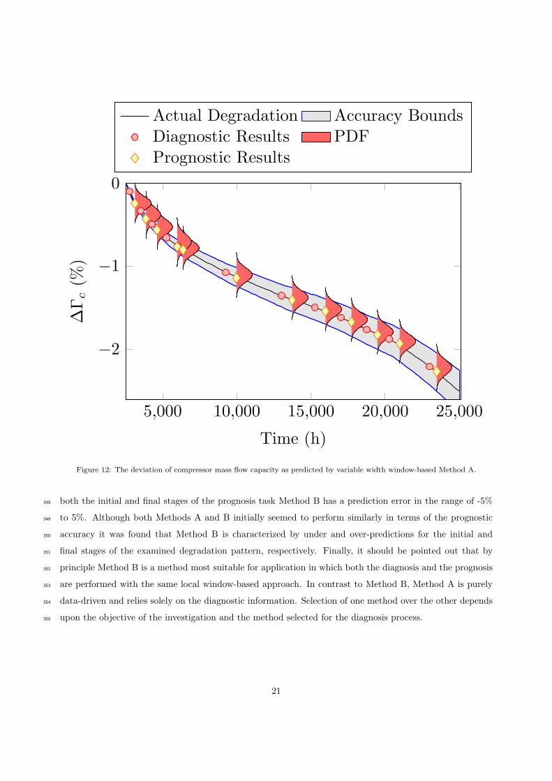
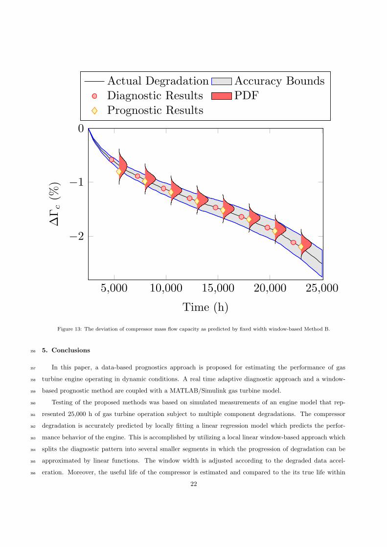
The deviation in compressor mass flow capacity as predicted by the Methods A and B is shown in325

Figs. 12 and 13, respectively. In the proposed method the prognosis task is performed more frequently326

than Method B. This is due to the number of windows used for capturing the diagnostic information. It is327

clear from Fig. 12, than the normal data distribution of the proposed prognostic method predictions fall328

within the accuracy bounds that were set at 90% of the actual degradation. On the other hand Method329

B presents similar performance with Method A apart from the first and final stages of the degradation330

pattern. One major advantage of the data-driven partitioning of the diagnostic pattern is that of linearizing331

the degradation trend and applying a local linear regression model for prognostics.332

The spread of the predicted mass flow capacity distribution depends on the gradient characterizing the333

diagnostic data that are contained in each window. As a result it is observed from Figs. 12 and 13 that334

19

5,000 10,000 15,000 20,000 25,000−3

−2

−1

0

1

2

3

4

56

7

8

9

Time (h)

∆Γc(%

)

Diagnostic Results Windows

Figure 11: Predicted compressor degradation represented by the deviation of the mass flow capacity. Diagnostic information

is splitted into 9 windows where their width is fixed.

especially for the first and last stages of the degradation pattern the spread is relatively higher than the335

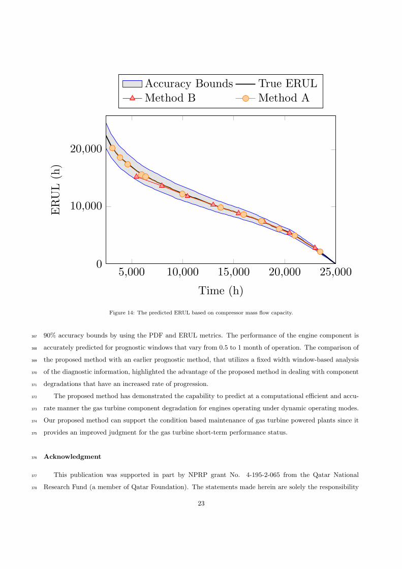
ones for the mid stages.336

An additional metric that facilitates the evaluation of the prognostic accuracy is that of the ERUL of337

the component based on its degradation. The predicted ERUL based on the compressor mass flow capacity338

is shown in Fig. 14 where the accuracy bounds refer to the true ERUL of the component. It is evident from339

Fig. 14 that the estimated ERUL falls within the accuracy bounds for all the local prognostic tasks for both340

Methods A and B. However, it is noticed from Fig. 14 that there is a small deviation in terms of ERUL341

between the two methods. The former observation can be amplified by examining the ERUL error of each342

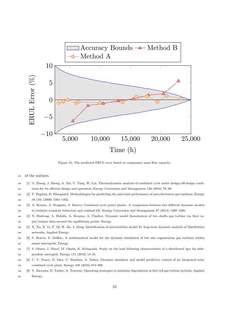
method.343

As expected the ERUL error of the Method A predictions lies consistently within the accuracy levels for344

all the time instants and ranges from 0% to 1.6%. On the other hand the error of Method B predictions345

might initially lie within the accuracy levels but at the final stages of the degradation pattern, where one346

would expect convergence to the true ERUL, the error increases. A closer look to Fig. 15 reveals that for347

20

5,000 10,000 15,000 20,000 25,000

−2

−1

0

Time (h)

∆Γc(%

)

Actual Degradation Accuracy BoundsDiagnostic Results PDFPrognostic Results

Figure 12: The deviation of compressor mass flow capacity as predicted by variable width window-based Method A.

both the initial and final stages of the prognosis task Method B has a prediction error in the range of -5%348

to 5%. Although both Methods A and B initially seemed to perform similarly in terms of the prognostic349

accuracy it was found that Method B is characterized by under and over-predictions for the initial and350

final stages of the examined degradation pattern, respectively. Finally, it should be pointed out that by351

principle Method B is a method most suitable for application in which both the diagnosis and the prognosis352

are performed with the same local window-based approach. In contrast to Method B, Method A is purely353

data-driven and relies solely on the diagnostic information. Selection of one method over the other depends354

upon the objective of the investigation and the method selected for the diagnosis process.355

21

5,000 10,000 15,000 20,000 25,000

−2

−1

0

Time (h)

∆Γc(%

)

Actual Degradation Accuracy BoundsDiagnostic Results PDFPrognostic Results

Figure 13: The deviation of compressor mass flow capacity as predicted by fixed width window-based Method B.

5. Conclusions356

In this paper, a data-based prognostics approach is proposed for estimating the performance of gas357

turbine engine operating in dynamic conditions. A real time adaptive diagnostic approach and a window-358

based prognostic method are coupled with a MATLAB/Simulink gas turbine model.359

Testing of the proposed methods was based on simulated measurements of an engine model that rep-360

resented 25,000 h of gas turbine operation subject to multiple component degradations. The compressor361

degradation is accurately predicted by locally fitting a linear regression model which predicts the perfor-362

mance behavior of the engine. This is accomplished by utilizing a local linear window-based approach which363

splits the diagnostic pattern into several smaller segments in which the progression of degradation can be364

approximated by linear functions. The window width is adjusted according to the degraded data accel-365

eration. Moreover, the useful life of the compressor is estimated and compared to the its true life within366

22

5,000 10,000 15,000 20,000 25,0000

10,000

20,000

Time (h)

ERUL(h)

Accuracy Bounds True ERULMethod B Method A

Figure 14: The predicted ERUL based on compressor mass flow capacity.

90% accuracy bounds by using the PDF and ERUL metrics. The performance of the engine component is367

accurately predicted for prognostic windows that vary from 0.5 to 1 month of operation. The comparison of368

the proposed method with an earlier prognostic method, that utilizes a fixed width window-based analysis369

of the diagnostic information, highlighted the advantage of the proposed method in dealing with component370

degradations that have an increased rate of progression.371

The proposed method has demonstrated the capability to predict at a computational efficient and accu-372

rate manner the gas turbine component degradation for engines operating under dynamic operating modes.373

Our proposed method can support the condition based maintenance of gas turbine powered plants since it374

provides an improved judgment for the gas turbine short-term performance status.375

Acknowledgment376

This publication was supported in part by NPRP grant No. 4-195-2-065 from the Qatar National377

Research Fund (a member of Qatar Foundation). The statements made herein are solely the responsibility378

23

5,000 10,000 15,000 20,000 25,000−10

−5

0

5

10

Time (h)

ERULError(%

)

Accuracy Bounds Method BMethod A

Figure 15: The predicted ERUL error based on compressor mass flow capacity.

of the authors.379

[1] G. Zhang, J. Zheng, A. Xie, Y. Yang, W. Liu, Thermodynamic analysis of combined cycle under design/off-design condi-380

tions for its efficient design and operation, Energy Conversion and Management 126 (2016) 76–88.381

[2] F. Haglind, B. Elmegaard, Methodologies for predicting the part-load performance of aero-derivative gas turbines, Energy382

34 (10) (2009) 1484–1492.383

[3] A. Benato, A. Stoppato, S. Bracco, Combined cycle power plants: A comparison between two different dynamic models384

to evaluate transient behaviour and residual life, Energy Conversion and Management 87 (2014) 1269–1280.385

[4] N. Hadroug, A. Hafaifa, A. Kouzou, A. Chaibet, Dynamic model linearization of two shafts gas turbine via their in-386

put/output data around the equilibrium points, Energy.387

[5] X. Xu, K. Li, F. Qi, H. Jia, J. Deng, Identification of microturbine model for long-term dynamic analysis of distribution388

networks, Applied Energy.389

[6] S. Bracco, F. Delfino, A mathematical model for the dynamic simulation of low size cogeneration gas turbines within390

smart microgrids, Energy.391

[7] S. Obara, J. Morel, M. Okada, K. Kobayashi, Study on the load following characteristics of a distributed igcc for inde-392

pendent microgrid, Energy 115 (2016) 13–25.393

[8] C. V. Ponce, D. Saez, C. Bordons, A. Nunez, Dynamic simulator and model predictive control of an integrated solar394

combined cycle plant, Energy 109 (2016) 974–986.395

[9] V. Zaccaria, D. Tucker, A. Traverso, Operating strategies to minimize degradation in fuel cell gas turbine hybrids, Applied396

Energy.397

24

[10] E. Tsoutsanis, N. Meskin, M. Benammar, K. Khorasani, A dynamic prognosis scheme for flexible operation of gas turbines,398

Applied Energy 164 (2016) 685–701.399

[11] A. Volponi, Gas turbine engine health management: Past, present, and future trends, Journal of Engineering for Gas400

Turbines and Power 136 (5) (2014) 051201.401

[12] J. Sun, H. Zuo, W. Wang, M. G. Pecht, Application of a state space modeling technique to system prognostics based402

on a health index for condition-based maintenance, Mechanical Systems and Signal Processing 28 (2012) 585 – 596,403

interdisciplinary and Integration Aspects in Structural Health Monitoring. doi:http://dx.doi.org/10.1016/j.ymssp.404

2011.09.029.405

URL http://www.sciencedirect.com/science/article/pii/S0888327011003979406

[13] D. Zhou, H. Zhang, Y.-G. Li, S. Weng, A dynamic reliability-centered maintenance analysis method for natural gas407

compressor station based on diagnostic and prognostic technology, Journal of Engineering for Gas Turbines and Power408

138 (6) (2016) 061601.409

[14] M. Y. Asr, M. M. Ettefagh, R. Hassannejad, S. N. Razavi, Diagnosis of combined faults in rotary machinery by non-naive410

bayesian approach, Mechanical Systems and Signal Processing 85 (2017) 56–70.411

[15] E. Mohammadi, M. Montazeri-Gh, Active fault tolerant control with self-enrichment capability for gas turbine engines,412

Aerospace Science and Technology 56 (2016) 70–89.413

[16] GE, Transforming GE to Digital Industrial, see also http://www.ge.com/ (2016).414

[17] Y. G. Li, A gas turbine diagnostic approach with transient measurements, Proceedings of the Institution of Mechanical415

Engineers, Part A: Journal of Power and Energy 217 (2) (2003) 169–177.416

[18] E. Tsoutsanis, N. Meskin, M. Benammar, K. Khorasani, Transient gas turbine performance diagnostics through nonlinear417

adaptation of compressor and turbine maps, Journal of Engineering for Gas Turbines and Power, GTP-14-1630 137.418

[19] G. Merrington, O. K. Kwon, G. Goodwin, B. Carlsson, Fault detection and diagnosis in gas turbines, Journal of Engineering419

for Gas Turbines and Power 113 (2) (1991) 276–282.420

[20] M. Amozegar, K. Khorasani, An ensemble of dynamic neural network identifiers for fault detection and isolation of gas421

turbine engines, Neural Networks 76 (2016) 106–121.422

[21] E. Mohammadi, M. Montazeri-Gh, A fuzzy-based gas turbine fault detection and identification system for full and part-load423

performance deterioration, Aerospace Science and Technology 46 (2015) 82–93.424

[22] A. Vatani, K. Khorasani, N. Meskin, Health monitoring and degradation prognostics in gas turbine engines using dynamic425

neural networks, in: ASME Turbo Expo, GT2015-4401, ASME, 2015.426

[23] J. Szoplik, Forecasting of natural gas consumption with artificial neural networks, Energy 85 (2015) 208 – 220. doi:http:427

//dx.doi.org/10.1016/j.energy.2015.03.084.428

URL http://www.sciencedirect.com/science/article/pii/S036054421500393X429

[24] M. A. Zaidan, R. F. Harrison, A. R. Mills, P. J. Fleming, Bayesian hierarchical models for aerospace gas turbine engine430

prognostics, Expert Systems with Applications 42 (1) (2015) 539 – 553.431

[25] M. A. Zaidan, A. R. Mills, R. F. Harrison, P. J. Fleming, Gas turbine engine prognostics using bayesian hierarchical432

models: A variational approach, Mechanical Systems and Signal Processing 7071 (2016) 120 – 140. doi:http://dx.doi.433

org/10.1016/j.ymssp.2015.09.014.434

URL http://www.sciencedirect.com/science/article/pii/S0888327015004094435

[26] D. Zhou, H. Zhang, S. Weng, A novel prognostic model of performance degradation trend for power machinery maintenance,436

Energy 78 (2014) 740 – 746. doi:http://dx.doi.org/10.1016/j.energy.2014.10.067.437

URL http://www.sciencedirect.com/science/article/pii/S0360544214012171438

[27] D. Feng, M. Xiao, Y. Liu, H. Song, Z. Yang, L. Zhang, A kernel principal component analysis–based degradation439

model and remaining useful life estimation for the turbofan engine, Advances in Mechanical Engineering 8 (5) (2016)440

25

1687814016650169.441

[28] E. Tsoutsanis, N. Meskin, M. Benammar, K. Khorasani, Performance-based prognosis scheme for industrial gas turbines,442

in: Prognostics and Health Management (PHM), 2015 IEEE Conference on, IEEE, 2015, pp. 1–8.443

[29] Y. G. Li, P. Nilkitsaranont, Gas turbine performance prognostic for condition-based maintenance, Applied Energy 86 (10)444

(2009) 2152–2161.445

[30] N. Daroogheh, N. Meskin, K. Khorasani, A novel particle filter parameter prediction scheme for failure prognosis, in:446

American Control Conference (ACC), 2014, IEEE, 2014, pp. 1735–1742.447

[31] N. Daroogheh, A. Baniamerian, N. Meskin, K. Khorasani, A hybrid prognosis and health monitoring strategy by integrating448

particle filters and neural networks for gas turbine engines, in: Prognostics and Health Management (PHM), 2015 IEEE449

Conference on, 2015, pp. 1–8. doi:10.1109/ICPHM.2015.7245020.450

[32] H. Hanachi, J. Liu, A. Banerjee, Y. Chen, Sequential state estimation of nonlinear/non-gaussian systems with stochastic451

input for turbine degradation estimation, Mechanical Systems and Signal Processing 72 (2016) 32–45.452

[33] Q. Wang, J. Huang, F. Lu, An improved particle filtering algorithm for aircraft engine gas-path fault diagnosis, Advances453

in Mechanical Engineering 8 (7) (2016) 1687814016659602.454

[34] D. E. Acuna, M. E. Orchard, Particle-filtering-based failure prognosis via sigma-points: Application to lithium-ion battery455

state-of-charge monitoring, Mechanical Systems and Signal Processing 85 (2017) 827–848.456

[35] D. Zhou, Z. Yu, H. Zhang, S. Weng, A novel grey prognostic model based on markov process and grey incidence analysis457

for energy conversion equipment degradation, Energy 109 (2016) 420 – 429. doi:http://dx.doi.org/10.1016/j.energy.458

2016.05.008.459

URL http://www.sciencedirect.com/science/article/pii/S0360544216305606460

[36] B. Pourbabaee, N. Meskin, K. Khorasani, Robust sensor fault detection and isolation of gas turbine engines subjected461

to time-varying parameter uncertainties, Mechanical Systems and Signal Processing (2016) –doi:http://dx.doi.org/10.462

1016/j.ymssp.2016.02.023.463

URL http://www.sciencedirect.com/science/article/pii/S0888327016000741464

[37] E. Tsoutsanis, N. Meskin, M. Benammar, K. Khorasani, A component map tuning method for performance prediction465

and diagnostics of gas turbine compressors, Applied Energy 135 (2014) 572–585.466

[38] E. Tsoutsanis, N. Meskin, Forecasting the health of gas turbine components through an integrated performance-based467

approach, in: Prognostics and Health Management (ICPHM), 2016 IEEE International Conference on, IEEE, 2016, pp.468

1–8.469

[39] A. Saxena, Prognostics the science of prediction, in: Proc. PHM Conference, Portland, OR, 2010.470

[40] Y. Cheng, C. Lu, T. Li, L. Tao, Residual lifetime prediction for lithium-ion battery based on functional principal component471

analysis and bayesian approach, Energy 90, Part 2 (2015) 1983 – 1993. doi:http://dx.doi.org/10.1016/j.energy.2015.472

07.022.473

URL http://www.sciencedirect.com/science/article/pii/S0360544215009172474

[41] K.-C. Yung, B. Sun, X. Jiang, Prognostics-based qualification of high-power white leds using levy process approach,475

Mechanical Systems and Signal Processing.476

[42] PROOSIS, Propulsion Object-Oriented Simulation Software, see also http://www.proosis.com/ (2016).477

[43] D. C. Montgomery, G. C. Runger, Applied statistics and probability for engineers, John Wiley & Sons, 2010.478

[44] L. Barelli, G. Bidini, A. Ottaviano, Integration of sofc/gt hybrid systems in micro-grids, Energy.479

[45] R. Chacartegui, D. Sanchez, A. Munoz, T. Sanchez, Real time simulation of medium size gas turbines, Energy Conversion480

and Management 52 (1) (2011) 713–724.481

[46] M. Sharifzadeh, M. Meghdari, D. Rashtchian, Multi-objective design and operation of solid oxide fuel cell (sofc) triple482

combined-cycle power generation systems: Integrating energy efficiency and operational safety, Applied Energy 185 (2017)483

26

345–361.484

[47] Y. Yu, L. Chen, F. Sun, C. Wu, Matlab/simulink-based simulation for digital-control system of marine three-shaft gas-485

turbine, Applied Energy 80 (1) (2005) 1–10.486

[48] GE, The LM2500+ Engine, see also http://www.ge.com/ (2017).487

[49] E. Tsoutsanis, N. Meskin, M. Benammar, K. Khorasani, Dynamic performance simulation of an aeroderivative gas turbine488

using the matlab simulink environment, in: Proc. ASME IMECE, IMECE2013-64102, Vol. 4, San Diego, USA, 2013, p.489

V04AT04A050.490

27