Embed Size (px)
Citation preview

Descent Algorithms, Line SearchLecturer: Pradeep Ravikumar
Co-instructor: Aarti Singh
Convex Optimization 10-725/36-725
Unconstrained Minimization
• To get to the optimal solution x^*, we typically use iterative algorithms
• Compute sequence of iterates x_k that (hopefully) converge to x^* at a fast rate
• x_{k+1} is some (simple) function of f, previous iterates
x
⇤ 2 argminx
f(x)
Two Classes of Iterative Algorithms
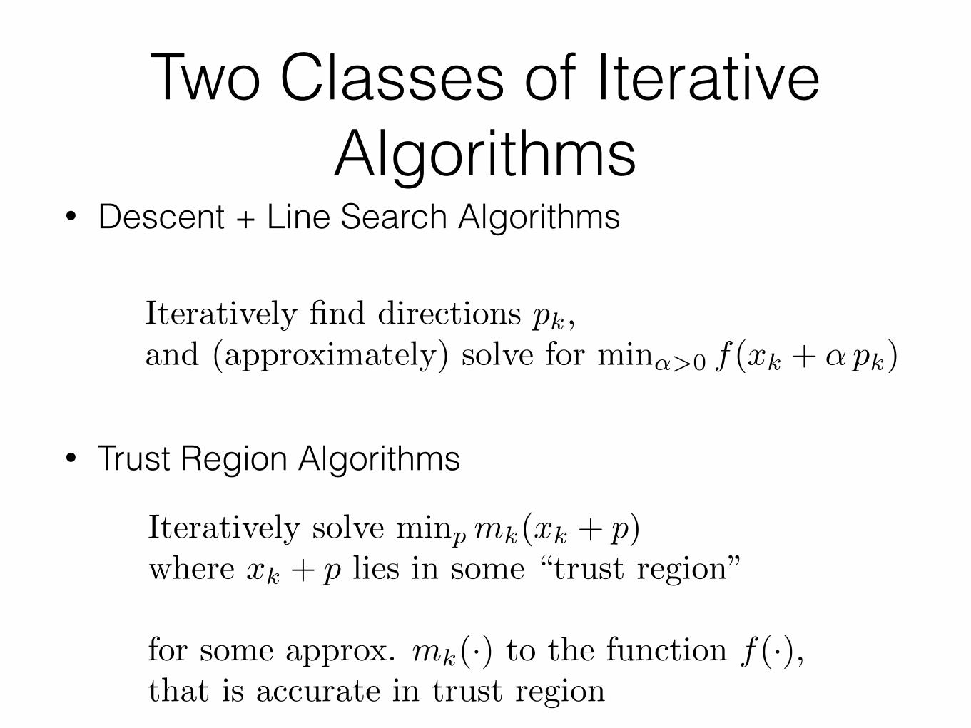
• Descent + Line Search Algorithms
• Trust Region Algorithms
Iteratively find directions pk,
and (approximately) solve for min↵>0 f(xk + ↵ pk)
Iteratively solve minp mk(xk + p)
where xk + p lies in some “trust region”
for some approx. mk(·) to the function f(·),that is accurate in trust region
Descent Algorithms
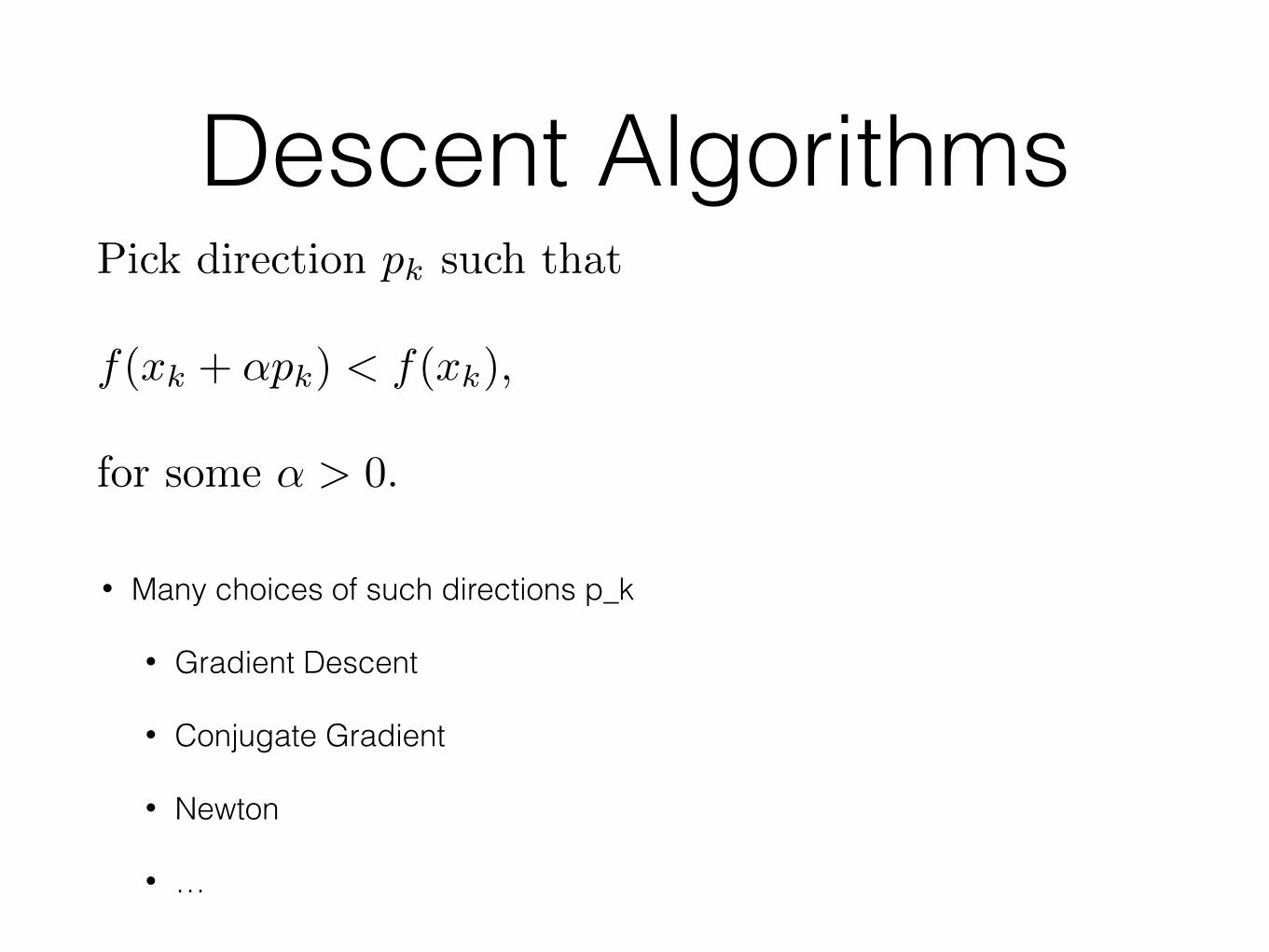
• Many choices of such directions p_k
• Gradient Descent
• Conjugate Gradient
• Newton
• …
Pick direction pk such that
f(xk + ↵pk) < f(xk),
for some ↵ > 0.
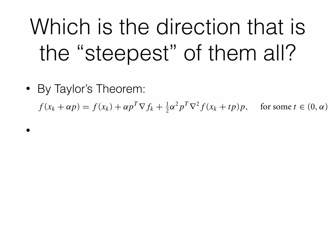
Which is the direction that is the “steepest” of them all?
• By Taylor’s Theorem:
•
2 . 2 . O v e r v i e w o f A l g o r i t h m s 21
contoursof model
of f
*
kunconstrainedminimizer
contours
pk
kp
x
1m =
m =12
Figure 2.4 Two possible trust regions (circles) and their corresponding steps pk . Thesolid lines are contours of the model function mk .
SEARCH DIRECTIONS FOR LINE SEARCH METHODS
The steepest-descent direction −∇fk is the most obvious choice for search directionfor a line search method. It is intuitive; among all the directions we could move from xk ,it is the one along which f decreases most rapidly. To verify this claim, we appeal again toTaylor’s theorem (Theorem 2.1), which tells us that for any search direction p and step-lengthparameter α, we have
f (xk + αp) # f (xk) + αpT∇fk + 12α
2pT∇2f (xk + tp)p, for some t ∈ (0,α)
(see (2.6)). The rate of change in f along the direction p at xk is simply the coefficient ofα, namely, pT∇fk . Hence, the unit direction p of most rapid decrease is the solution to theproblem
minp
pT∇fk, subject to ∥p∥ # 1. (2.12)
Since pT∇fk # ∥p∥ ∥∇fk∥ cos θ , where θ is the angle between p and ∇fk , we have from∥p∥ # 1 that pT∇fk # ∥∇fk∥ cos θ , so the objective in (2.12) is minimized when cos θ

Which is the direction that is the “steepest” of them all?
• By Taylor’s Theorem:
• Rate of change of f along direction p:
2 . 2 . O v e r v i e w o f A l g o r i t h m s 21
contoursof model
of f
*
kunconstrainedminimizer
contours
pk
kp
x
1m =
m =12
Figure 2.4 Two possible trust regions (circles) and their corresponding steps pk . Thesolid lines are contours of the model function mk .
SEARCH DIRECTIONS FOR LINE SEARCH METHODS
The steepest-descent direction −∇fk is the most obvious choice for search directionfor a line search method. It is intuitive; among all the directions we could move from xk ,it is the one along which f decreases most rapidly. To verify this claim, we appeal again toTaylor’s theorem (Theorem 2.1), which tells us that for any search direction p and step-lengthparameter α, we have
f (xk + αp) # f (xk) + αpT∇fk + 12α
2pT∇2f (xk + tp)p, for some t ∈ (0,α)
(see (2.6)). The rate of change in f along the direction p at xk is simply the coefficient ofα, namely, pT∇fk . Hence, the unit direction p of most rapid decrease is the solution to theproblem
minp
pT∇fk, subject to ∥p∥ # 1. (2.12)
Since pT∇fk # ∥p∥ ∥∇fk∥ cos θ , where θ is the angle between p and ∇fk , we have from∥p∥ # 1 that pT∇fk # ∥∇fk∥ cos θ , so the objective in (2.12) is minimized when cos θ
lim↵!0
f(xk + ↵p)� f(xk)
↵
= p
T rfk

Which is the direction that is the “steepest” of them all?
• By Taylor’s Theorem:
• Rate of change of f along direction p:
• Unit direction p with most rapid decrease:
2 . 2 . O v e r v i e w o f A l g o r i t h m s 21
contoursof model
of f
*
kunconstrainedminimizer
contours
pk
kp
x
1m =
m =12
Figure 2.4 Two possible trust regions (circles) and their corresponding steps pk . Thesolid lines are contours of the model function mk .
SEARCH DIRECTIONS FOR LINE SEARCH METHODS
The steepest-descent direction −∇fk is the most obvious choice for search directionfor a line search method. It is intuitive; among all the directions we could move from xk ,it is the one along which f decreases most rapidly. To verify this claim, we appeal again toTaylor’s theorem (Theorem 2.1), which tells us that for any search direction p and step-lengthparameter α, we have
f (xk + αp) # f (xk) + αpT∇fk + 12α
2pT∇2f (xk + tp)p, for some t ∈ (0,α)
(see (2.6)). The rate of change in f along the direction p at xk is simply the coefficient ofα, namely, pT∇fk . Hence, the unit direction p of most rapid decrease is the solution to theproblem
minp
pT∇fk, subject to ∥p∥ # 1. (2.12)
Since pT∇fk # ∥p∥ ∥∇fk∥ cos θ , where θ is the angle between p and ∇fk , we have from∥p∥ # 1 that pT∇fk # ∥∇fk∥ cos θ , so the objective in (2.12) is minimized when cos θ
lim↵!0
f(xk + ↵p)� f(xk)
↵
= p
T rfk
2 . 2 . O v e r v i e w o f A l g o r i t h m s 21
contoursof model
of f
*
kunconstrainedminimizer
contours
pk
kp
x
1m =
m =12
Figure 2.4 Two possible trust regions (circles) and their corresponding steps pk . Thesolid lines are contours of the model function mk .
SEARCH DIRECTIONS FOR LINE SEARCH METHODS
The steepest-descent direction −∇fk is the most obvious choice for search directionfor a line search method. It is intuitive; among all the directions we could move from xk ,it is the one along which f decreases most rapidly. To verify this claim, we appeal again toTaylor’s theorem (Theorem 2.1), which tells us that for any search direction p and step-lengthparameter α, we have
f (xk + αp) # f (xk) + αpT∇fk + 12α
2pT∇2f (xk + tp)p, for some t ∈ (0,α)
(see (2.6)). The rate of change in f along the direction p at xk is simply the coefficient ofα, namely, pT∇fk . Hence, the unit direction p of most rapid decrease is the solution to theproblem
minp
pT∇fk, subject to ∥p∥ # 1. (2.12)
Since pT∇fk # ∥p∥ ∥∇fk∥ cos θ , where θ is the angle between p and ∇fk , we have from∥p∥ # 1 that pT∇fk # ∥∇fk∥ cos θ , so the objective in (2.12) is minimized when cos θ

Which is the direction that is the “steepest” of them all?
• By Taylor’s Theorem:
• Rate of change of f along direction p:
• Unit direction p with most rapid decrease:
2 . 2 . O v e r v i e w o f A l g o r i t h m s 21
contoursof model
of f
*
kunconstrainedminimizer
contours
pk
kp
x
1m =
m =12
Figure 2.4 Two possible trust regions (circles) and their corresponding steps pk . Thesolid lines are contours of the model function mk .
SEARCH DIRECTIONS FOR LINE SEARCH METHODS
The steepest-descent direction −∇fk is the most obvious choice for search directionfor a line search method. It is intuitive; among all the directions we could move from xk ,it is the one along which f decreases most rapidly. To verify this claim, we appeal again toTaylor’s theorem (Theorem 2.1), which tells us that for any search direction p and step-lengthparameter α, we have
f (xk + αp) # f (xk) + αpT∇fk + 12α
2pT∇2f (xk + tp)p, for some t ∈ (0,α)
(see (2.6)). The rate of change in f along the direction p at xk is simply the coefficient ofα, namely, pT∇fk . Hence, the unit direction p of most rapid decrease is the solution to theproblem
minp
pT∇fk, subject to ∥p∥ # 1. (2.12)
Since pT∇fk # ∥p∥ ∥∇fk∥ cos θ , where θ is the angle between p and ∇fk , we have from∥p∥ # 1 that pT∇fk # ∥∇fk∥ cos θ , so the objective in (2.12) is minimized when cos θ
lim↵!0
f(xk + ↵p)� f(xk)
↵
= p
T rfk
22 C h a p t e r 2 . F u n d a m e n t a l s o f U n c o n s t r a i n e d O p t i m i z a t i o n
kx
kp *x.
Figure 2.5 Steepest descent direction for a function of two variables.
takes on its minimum value of−1 at θ " π radians. In other words, the solution to (2.12) is
p " −∇fk/∥∇fk∥,
as claimed. As we show in Figure 2.5, this direction is orthogonal to the contours of thefunction.
The steepest descent method is a line search method that moves along pk " −∇fk atevery step. It can choose the step lengthαk in a variety of ways, as we discuss in Chapter 3. Oneadvantage of the steepest descent direction is that it requires calculation of the gradient ∇fk
but not of second derivatives. However, it can be excruciatingly slow on difficult problems.Line search methods may use search directions other than the steepest descent direc-
tion. In general, any descent direction—one that makes an angle of strictly less than π/2radians with−∇fk—is guaranteed to produce a decrease in f , provided that the step lengthis sufficiently small (see Figure 2.6). We can verify this claim by using Taylor’s theorem. From(2.6), we have that
f (xk + ϵpk) " f (xk) + ϵpTk ∇fk + O(ϵ2).
When pk is a downhill direction, the angle θk between pk and ∇fk has cos θk < 0, so that
pTk ∇fk " ∥pk∥ ∥∇fk∥ cos θk < 0.
It follows that f (xk + ϵpk) < f (xk) for all positive but sufficiently small values of ϵ.Another important search direction—perhaps the most important one of all—
is the Newton direction. This direction is derived from the second-order Taylor series
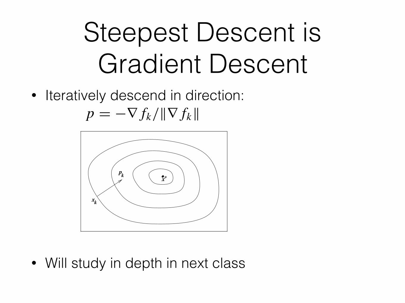
Steepest Descent is Gradient Descent
• Iteratively descend in direction:
• Will study in depth in next class
22 C h a p t e r 2 . F u n d a m e n t a l s o f U n c o n s t r a i n e d O p t i m i z a t i o n
kx
kp *x.
Figure 2.5 Steepest descent direction for a function of two variables.
takes on its minimum value of−1 at θ " π radians. In other words, the solution to (2.12) is
p " −∇fk/∥∇fk∥,
as claimed. As we show in Figure 2.5, this direction is orthogonal to the contours of thefunction.
The steepest descent method is a line search method that moves along pk " −∇fk atevery step. It can choose the step lengthαk in a variety of ways, as we discuss in Chapter 3. Oneadvantage of the steepest descent direction is that it requires calculation of the gradient ∇fk
but not of second derivatives. However, it can be excruciatingly slow on difficult problems.Line search methods may use search directions other than the steepest descent direc-
tion. In general, any descent direction—one that makes an angle of strictly less than π/2radians with−∇fk—is guaranteed to produce a decrease in f , provided that the step lengthis sufficiently small (see Figure 2.6). We can verify this claim by using Taylor’s theorem. From(2.6), we have that
f (xk + ϵpk) " f (xk) + ϵpTk ∇fk + O(ϵ2).
When pk is a downhill direction, the angle θk between pk and ∇fk has cos θk < 0, so that
pTk ∇fk " ∥pk∥ ∥∇fk∥ cos θk < 0.
It follows that f (xk + ϵpk) < f (xk) for all positive but sufficiently small values of ϵ.Another important search direction—perhaps the most important one of all—
is the Newton direction. This direction is derived from the second-order Taylor series
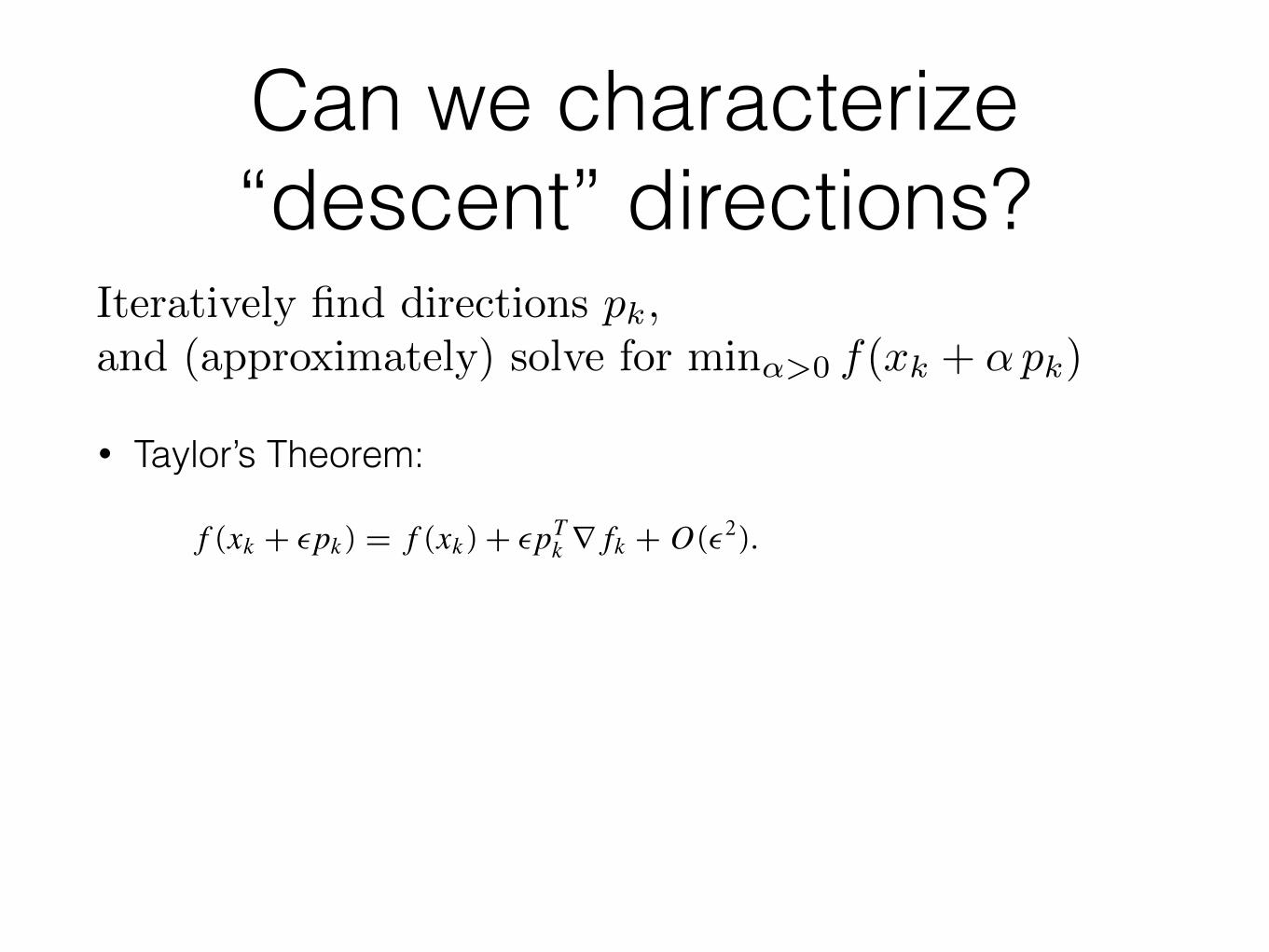
Can we characterize “descent” directions?
• Taylor’s Theorem:
Iteratively find directions pk,
and (approximately) solve for min↵>0 f(xk + ↵ pk)
22 C h a p t e r 2 . F u n d a m e n t a l s o f U n c o n s t r a i n e d O p t i m i z a t i o n
kx
kp *x.
Figure 2.5 Steepest descent direction for a function of two variables.
takes on its minimum value of−1 at θ " π radians. In other words, the solution to (2.12) is
p " −∇fk/∥∇fk∥,
as claimed. As we show in Figure 2.5, this direction is orthogonal to the contours of thefunction.
The steepest descent method is a line search method that moves along pk " −∇fk atevery step. It can choose the step lengthαk in a variety of ways, as we discuss in Chapter 3. Oneadvantage of the steepest descent direction is that it requires calculation of the gradient ∇fk
but not of second derivatives. However, it can be excruciatingly slow on difficult problems.Line search methods may use search directions other than the steepest descent direc-
tion. In general, any descent direction—one that makes an angle of strictly less than π/2radians with−∇fk—is guaranteed to produce a decrease in f , provided that the step lengthis sufficiently small (see Figure 2.6). We can verify this claim by using Taylor’s theorem. From(2.6), we have that
f (xk + ϵpk) " f (xk) + ϵpTk ∇fk + O(ϵ2).
When pk is a downhill direction, the angle θk between pk and ∇fk has cos θk < 0, so that
pTk ∇fk " ∥pk∥ ∥∇fk∥ cos θk < 0.
It follows that f (xk + ϵpk) < f (xk) for all positive but sufficiently small values of ϵ.Another important search direction—perhaps the most important one of all—
is the Newton direction. This direction is derived from the second-order Taylor series

Can we characterize “descent” directions?
• Taylor’s Theorem:
• Suppose angle between p_k and \grad f_k is \theta_k, and cos(\theta_k) < 0 i.e. angle is strictly less than 90 degrees
Iteratively find directions pk,
and (approximately) solve for min↵>0 f(xk + ↵ pk)
22 C h a p t e r 2 . F u n d a m e n t a l s o f U n c o n s t r a i n e d O p t i m i z a t i o n
kx
kp *x.
Figure 2.5 Steepest descent direction for a function of two variables.
takes on its minimum value of−1 at θ " π radians. In other words, the solution to (2.12) is
p " −∇fk/∥∇fk∥,
as claimed. As we show in Figure 2.5, this direction is orthogonal to the contours of thefunction.
The steepest descent method is a line search method that moves along pk " −∇fk atevery step. It can choose the step lengthαk in a variety of ways, as we discuss in Chapter 3. Oneadvantage of the steepest descent direction is that it requires calculation of the gradient ∇fk
but not of second derivatives. However, it can be excruciatingly slow on difficult problems.Line search methods may use search directions other than the steepest descent direc-
tion. In general, any descent direction—one that makes an angle of strictly less than π/2radians with−∇fk—is guaranteed to produce a decrease in f , provided that the step lengthis sufficiently small (see Figure 2.6). We can verify this claim by using Taylor’s theorem. From(2.6), we have that
f (xk + ϵpk) " f (xk) + ϵpTk ∇fk + O(ϵ2).
When pk is a downhill direction, the angle θk between pk and ∇fk has cos θk < 0, so that
pTk ∇fk " ∥pk∥ ∥∇fk∥ cos θk < 0.
It follows that f (xk + ϵpk) < f (xk) for all positive but sufficiently small values of ϵ.Another important search direction—perhaps the most important one of all—
is the Newton direction. This direction is derived from the second-order Taylor series
))
22 C h a p t e r 2 . F u n d a m e n t a l s o f U n c o n s t r a i n e d O p t i m i z a t i o n
kx
kp *x.
Figure 2.5 Steepest descent direction for a function of two variables.
takes on its minimum value of−1 at θ " π radians. In other words, the solution to (2.12) is
p " −∇fk/∥∇fk∥,
as claimed. As we show in Figure 2.5, this direction is orthogonal to the contours of thefunction.
The steepest descent method is a line search method that moves along pk " −∇fk atevery step. It can choose the step lengthαk in a variety of ways, as we discuss in Chapter 3. Oneadvantage of the steepest descent direction is that it requires calculation of the gradient ∇fk
but not of second derivatives. However, it can be excruciatingly slow on difficult problems.Line search methods may use search directions other than the steepest descent direc-
tion. In general, any descent direction—one that makes an angle of strictly less than π/2radians with−∇fk—is guaranteed to produce a decrease in f , provided that the step lengthis sufficiently small (see Figure 2.6). We can verify this claim by using Taylor’s theorem. From(2.6), we have that
f (xk + ϵpk) " f (xk) + ϵpTk ∇fk + O(ϵ2).
When pk is a downhill direction, the angle θk between pk and ∇fk has cos θk < 0, so that
pTk ∇fk " ∥pk∥ ∥∇fk∥ cos θk < 0.
It follows that f (xk + ϵpk) < f (xk) for all positive but sufficiently small values of ϵ.Another important search direction—perhaps the most important one of all—
is the Newton direction. This direction is derived from the second-order Taylor series
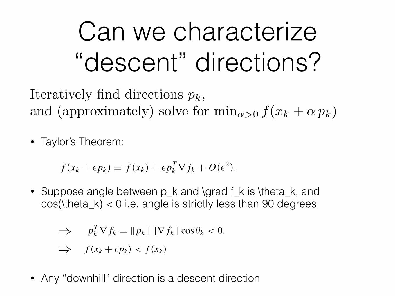
Can we characterize “descent” directions?
• Taylor’s Theorem:
• Suppose angle between p_k and \grad f_k is \theta_k, and cos(\theta_k) < 0 i.e. angle is strictly less than 90 degrees
• Any “downhill” direction is a descent direction
Iteratively find directions pk,
and (approximately) solve for min↵>0 f(xk + ↵ pk)
22 C h a p t e r 2 . F u n d a m e n t a l s o f U n c o n s t r a i n e d O p t i m i z a t i o n
kx
kp *x.
Figure 2.5 Steepest descent direction for a function of two variables.
takes on its minimum value of−1 at θ " π radians. In other words, the solution to (2.12) is
p " −∇fk/∥∇fk∥,
as claimed. As we show in Figure 2.5, this direction is orthogonal to the contours of thefunction.
The steepest descent method is a line search method that moves along pk " −∇fk atevery step. It can choose the step lengthαk in a variety of ways, as we discuss in Chapter 3. Oneadvantage of the steepest descent direction is that it requires calculation of the gradient ∇fk
but not of second derivatives. However, it can be excruciatingly slow on difficult problems.Line search methods may use search directions other than the steepest descent direc-
tion. In general, any descent direction—one that makes an angle of strictly less than π/2radians with−∇fk—is guaranteed to produce a decrease in f , provided that the step lengthis sufficiently small (see Figure 2.6). We can verify this claim by using Taylor’s theorem. From(2.6), we have that
f (xk + ϵpk) " f (xk) + ϵpTk ∇fk + O(ϵ2).
When pk is a downhill direction, the angle θk between pk and ∇fk has cos θk < 0, so that
pTk ∇fk " ∥pk∥ ∥∇fk∥ cos θk < 0.
It follows that f (xk + ϵpk) < f (xk) for all positive but sufficiently small values of ϵ.Another important search direction—perhaps the most important one of all—
is the Newton direction. This direction is derived from the second-order Taylor series
22 C h a p t e r 2 . F u n d a m e n t a l s o f U n c o n s t r a i n e d O p t i m i z a t i o n
kx
kp *x.
Figure 2.5 Steepest descent direction for a function of two variables.
takes on its minimum value of−1 at θ " π radians. In other words, the solution to (2.12) is
p " −∇fk/∥∇fk∥,
as claimed. As we show in Figure 2.5, this direction is orthogonal to the contours of thefunction.
The steepest descent method is a line search method that moves along pk " −∇fk atevery step. It can choose the step lengthαk in a variety of ways, as we discuss in Chapter 3. Oneadvantage of the steepest descent direction is that it requires calculation of the gradient ∇fk
but not of second derivatives. However, it can be excruciatingly slow on difficult problems.Line search methods may use search directions other than the steepest descent direc-
tion. In general, any descent direction—one that makes an angle of strictly less than π/2radians with−∇fk—is guaranteed to produce a decrease in f , provided that the step lengthis sufficiently small (see Figure 2.6). We can verify this claim by using Taylor’s theorem. From(2.6), we have that
f (xk + ϵpk) " f (xk) + ϵpTk ∇fk + O(ϵ2).
When pk is a downhill direction, the angle θk between pk and ∇fk has cos θk < 0, so that
pTk ∇fk " ∥pk∥ ∥∇fk∥ cos θk < 0.
It follows that f (xk + ϵpk) < f (xk) for all positive but sufficiently small values of ϵ.Another important search direction—perhaps the most important one of all—
is the Newton direction. This direction is derived from the second-order Taylor series
))
22 C h a p t e r 2 . F u n d a m e n t a l s o f U n c o n s t r a i n e d O p t i m i z a t i o n
kx
kp *x.
Figure 2.5 Steepest descent direction for a function of two variables.
takes on its minimum value of−1 at θ " π radians. In other words, the solution to (2.12) is
p " −∇fk/∥∇fk∥,
as claimed. As we show in Figure 2.5, this direction is orthogonal to the contours of thefunction.
The steepest descent method is a line search method that moves along pk " −∇fk atevery step. It can choose the step lengthαk in a variety of ways, as we discuss in Chapter 3. Oneadvantage of the steepest descent direction is that it requires calculation of the gradient ∇fk
but not of second derivatives. However, it can be excruciatingly slow on difficult problems.Line search methods may use search directions other than the steepest descent direc-
tion. In general, any descent direction—one that makes an angle of strictly less than π/2radians with−∇fk—is guaranteed to produce a decrease in f , provided that the step lengthis sufficiently small (see Figure 2.6). We can verify this claim by using Taylor’s theorem. From(2.6), we have that
f (xk + ϵpk) " f (xk) + ϵpTk ∇fk + O(ϵ2).
When pk is a downhill direction, the angle θk between pk and ∇fk has cos θk < 0, so that
pTk ∇fk " ∥pk∥ ∥∇fk∥ cos θk < 0.
It follows that f (xk + ϵpk) < f (xk) for all positive but sufficiently small values of ϵ.Another important search direction—perhaps the most important one of all—
is the Newton direction. This direction is derived from the second-order Taylor series

Can we characterize “descent” directions?
Iteratively find directions pk,
and (approximately) solve for min↵>0 f(xk + ↵ pk)2 . 2 . O v e r v i e w o f A l g o r i t h m s 23
_kf
pk
Figure 2.6 A downhill direction pk
approximation to f (xk + p), which is
f (xk + p) ≈ fk + pT∇fk + 12p
T∇2fkpdef# mk(p). (2.13)
Assuming for the moment that ∇2fk is positive definite, we obtain the Newton directionby finding the vector p that minimizes mk(p). By simply setting the derivative of mk(p) tozero, we obtain the following explicit formula:
pNk # −∇2f −1
k ∇fk. (2.14)
The Newton direction is reliable when the difference between the true function f (xk +p) and its quadratic model mk(p) is not too large. By comparing (2.13) with (2.6), we seethat the only difference between these functions is that the matrix ∇2f (xk + tp) in thethird term of the expansion has been replaced by ∇2fk # ∇2f (xk). If ∇2f (·) is sufficientlysmooth, this difference introduces a perturbation of only O(∥p∥3) into the expansion, sothat when ∥p∥ is small, the approximation f (xk + p) ≈ mk(p) is very accurate indeed.
The Newton direction can be used in a line search method when ∇2fk is positivedefinite, for in this case we have
∇f Tk pN
k # −pNkT∇2fkp
Nk ≤ −σk∥pN
k∥2
for some σk > 0. Unless the gradient ∇fk (and therefore the step pNk ) is zero, we have that
∇f Tk pN
k < 0, so the Newton direction is a descent direction. Unlike the steepest descentdirection, there is a “natural” step length of 1 associated with the Newton direction. Most
Downhill direction p_k
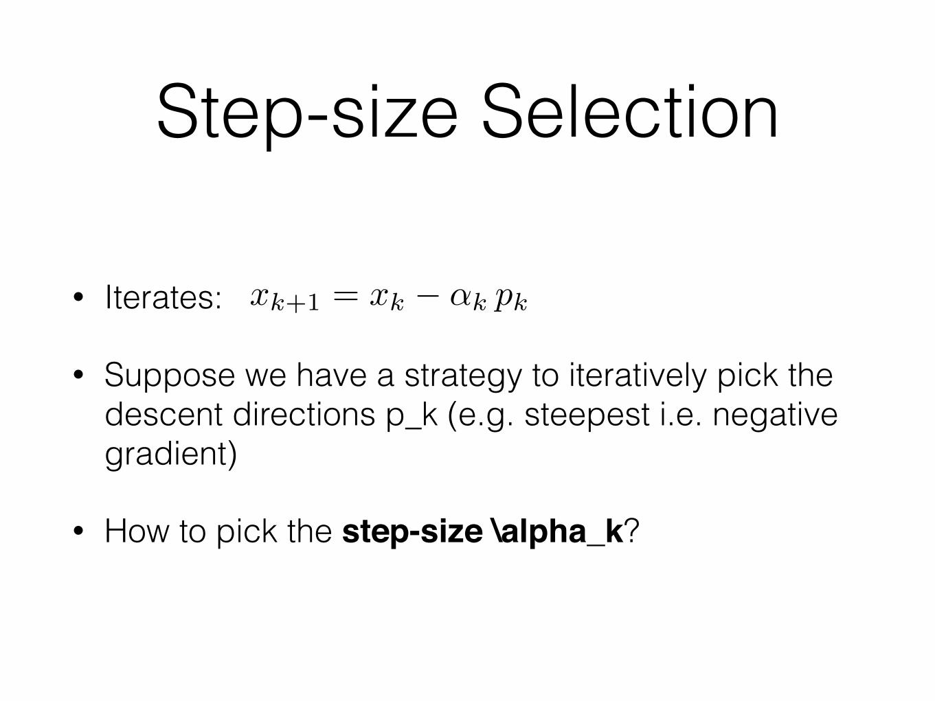
Step-size Selection
• Iterates:
• Suppose we have a strategy to iteratively pick the descent directions p_k (e.g. steepest i.e. negative gradient)
• How to pick the step-size \alpha_k?
xk+1 = xk � ↵k pk
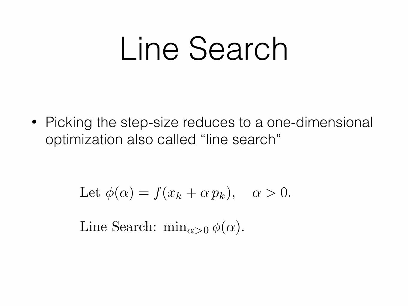
Line Search
• Picking the step-size reduces to a one-dimensional optimization also called “line search”
Let �(↵) = f(xk + ↵ pk), ↵ > 0.
Line Search: min↵>0 �(↵).

Exact Line Search
• One-dimensional non-convex optimization problem
• Might be too expensive
Solve for global minimum: min↵>0 �(↵).36 C h a p t e r 3 . L i n e S e a r c h M e t h o d s
(φ α)
pointstationaryfirst
minimizerlocalfirst
global minimizer
α
Figure 3.1 The ideal step length is the global minimizer.
iteration by means of a low-rank formula. When pk is defined by (3.2) and Bk is positivedefinite, we have
pTk ∇fk " −∇f T
k B−1k ∇fk < 0,
and therefore pk is a descent direction.In the next chapters we study how to choose the matrix Bk , or more generally, how
to compute the search direction. We now give careful consideration to the choice of thestep-length parameter αk .
3.1 STEP LENGTH
In computing the step length αk , we face a tradeoff. We would like to choose αk togive a substantial reduction of f , but at the same time, we do not want to spend too muchtime making the choice. The ideal choice would be the global minimizer of the univariatefunction φ(·) defined by
φ(α) " f (xk + αpk), α > 0, (3.3)
but in general, it is too expensive to identify this value (see Figure 3.1). To find even a localminimizer of φ to moderate precision generally requires too many evaluations of the objec-
Inexact line search• Solve for the optimization min_{alpha > 0}
\phi(alpha) approximately and cheaply
• Question: is it sufficient to obtain an alpha that strictly?
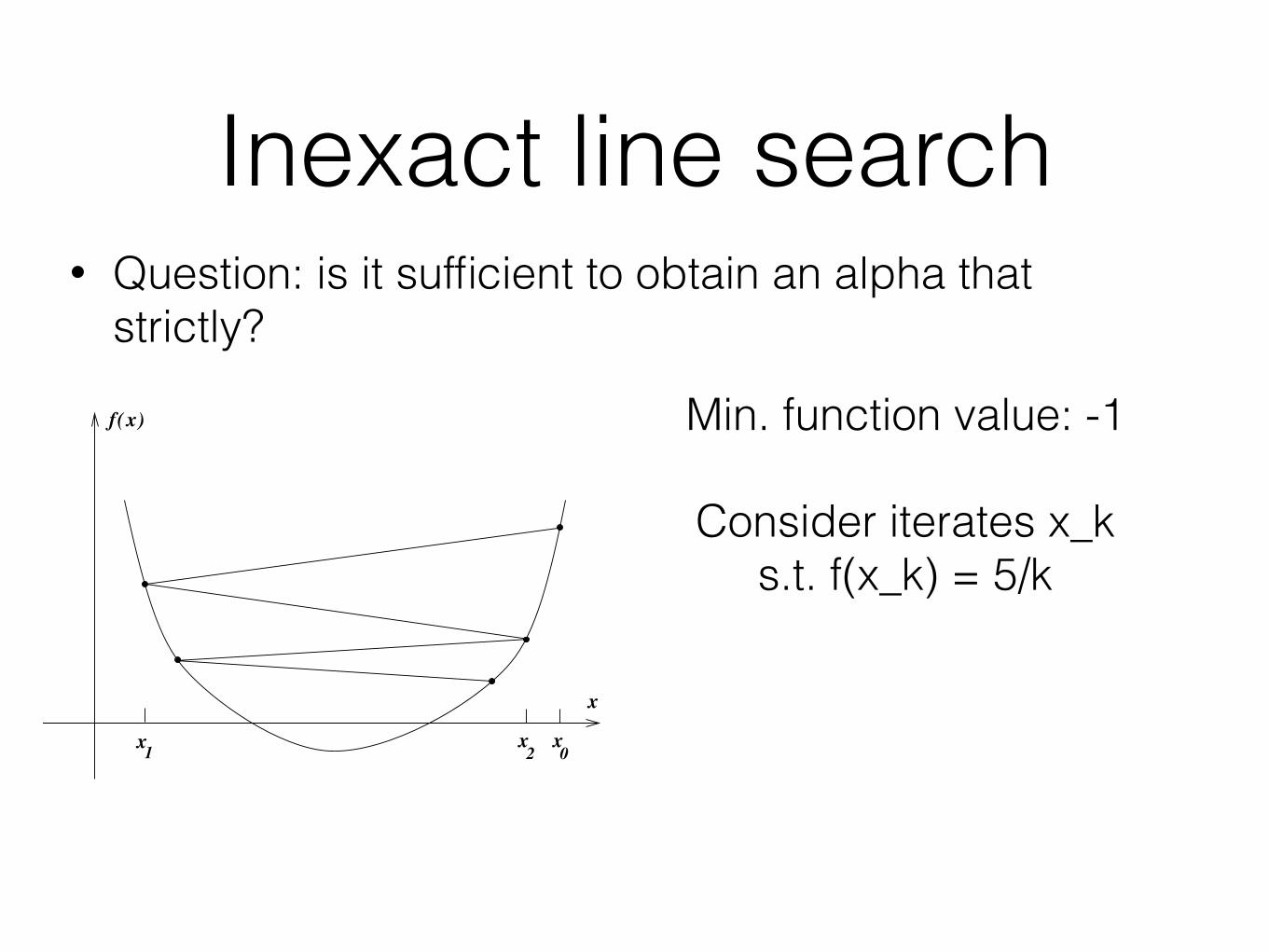
Inexact line search• Question: is it sufficient to obtain an alpha that
strictly? 3 . 1 . S t e p L e n g t h 37
2x
0x1x
x
xf( )
Figure 3.2 Insufficient reduction in f .
tive function f and possibly the gradient ∇f . More practical strategies perform an inexactline search to identify a step length that achieves adequate reductions in f at minimal cost.
Typical line search algorithms try out a sequence of candidate values for α, stopping toaccept one of these values when certain conditions are satisfied. The line search is done in twostages: A bracketing phase finds an interval containing desirable step lengths, and a bisectionor interpolation phase computes a good step length within this interval. Sophisticated linesearch algorithms can be quite complicated, so we defer a full description until the end ofthis chapter. We now discuss various termination conditions for the line search algorithmand show that effective step lengths need not lie near minimizers of the univariate functionφ(α) defined in (3.3).
A simple condition we could impose on αk is that it provide a reduction in f , i.e.,f (xk + αkpk) < f (xk). That this is not appropriate is illustrated in Figure 3.2, where theminimum is f ∗ # −1, but the sequence of function values {5/k}, k # 0, 1, . . ., convergesto zero. The difficulty is that we do not have sufficient reduction in f , a concept we discussnext.
THE WOLFE CONDITIONS
A popular inexact line search condition stipulates thatαk should first of all give sufficientdecrease in the objective function f , as measured by the following inequality:
f (xk + αpk) ≤ f (xk) + c1α∇f Tk pk, (3.4)
Min. function value: -1
Consider iterates x_k s.t. f(x_k) = 5/k
Inexact line search• Question: is it sufficient to obtain an alpha that
strictly? 3 . 1 . S t e p L e n g t h 37
2x
0x1x
x
xf( )
Figure 3.2 Insufficient reduction in f .
tive function f and possibly the gradient ∇f . More practical strategies perform an inexactline search to identify a step length that achieves adequate reductions in f at minimal cost.
Typical line search algorithms try out a sequence of candidate values for α, stopping toaccept one of these values when certain conditions are satisfied. The line search is done in twostages: A bracketing phase finds an interval containing desirable step lengths, and a bisectionor interpolation phase computes a good step length within this interval. Sophisticated linesearch algorithms can be quite complicated, so we defer a full description until the end ofthis chapter. We now discuss various termination conditions for the line search algorithmand show that effective step lengths need not lie near minimizers of the univariate functionφ(α) defined in (3.3).
A simple condition we could impose on αk is that it provide a reduction in f , i.e.,f (xk + αkpk) < f (xk). That this is not appropriate is illustrated in Figure 3.2, where theminimum is f ∗ # −1, but the sequence of function values {5/k}, k # 0, 1, . . ., convergesto zero. The difficulty is that we do not have sufficient reduction in f , a concept we discussnext.
THE WOLFE CONDITIONS
A popular inexact line search condition stipulates thatαk should first of all give sufficientdecrease in the objective function f , as measured by the following inequality:
f (xk + αpk) ≤ f (xk) + c1α∇f Tk pk, (3.4)
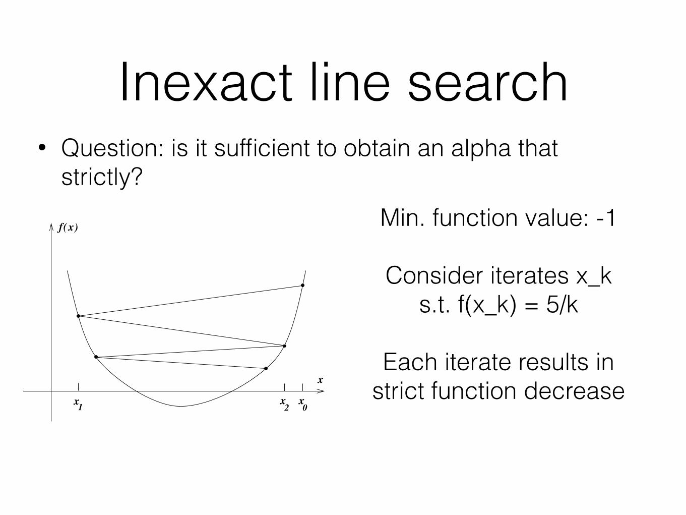
Min. function value: -1
Consider iterates x_k s.t. f(x_k) = 5/k
Each iterate results in strict function decrease

Inexact line search• Question: is it sufficient to obtain an alpha that
strictly? 3 . 1 . S t e p L e n g t h 37
2x
0x1x
x
xf( )
Figure 3.2 Insufficient reduction in f .
tive function f and possibly the gradient ∇f . More practical strategies perform an inexactline search to identify a step length that achieves adequate reductions in f at minimal cost.
Typical line search algorithms try out a sequence of candidate values for α, stopping toaccept one of these values when certain conditions are satisfied. The line search is done in twostages: A bracketing phase finds an interval containing desirable step lengths, and a bisectionor interpolation phase computes a good step length within this interval. Sophisticated linesearch algorithms can be quite complicated, so we defer a full description until the end ofthis chapter. We now discuss various termination conditions for the line search algorithmand show that effective step lengths need not lie near minimizers of the univariate functionφ(α) defined in (3.3).
A simple condition we could impose on αk is that it provide a reduction in f , i.e.,f (xk + αkpk) < f (xk). That this is not appropriate is illustrated in Figure 3.2, where theminimum is f ∗ # −1, but the sequence of function values {5/k}, k # 0, 1, . . ., convergesto zero. The difficulty is that we do not have sufficient reduction in f , a concept we discussnext.
THE WOLFE CONDITIONS
A popular inexact line search condition stipulates thatαk should first of all give sufficientdecrease in the objective function f , as measured by the following inequality:
f (xk + αpk) ≤ f (xk) + c1α∇f Tk pk, (3.4)
Consider iterates x_k s.t. f(x_k) = 5/k
Each iterate results in strict function decrease
But f(x_k) converges to zero, which is greater than min. value which is -1
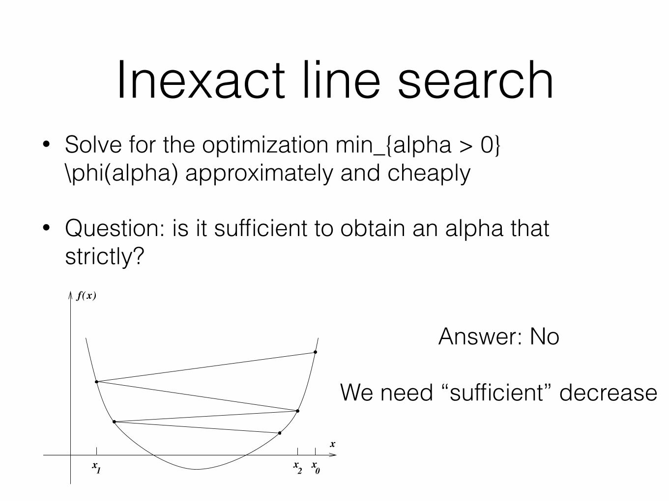
Inexact line search• Solve for the optimization min_{alpha > 0}
\phi(alpha) approximately and cheaply
• Question: is it sufficient to obtain an alpha that strictly? 3 . 1 . S t e p L e n g t h 37
2x
0x1x
x
xf( )
Figure 3.2 Insufficient reduction in f .
tive function f and possibly the gradient ∇f . More practical strategies perform an inexactline search to identify a step length that achieves adequate reductions in f at minimal cost.
Typical line search algorithms try out a sequence of candidate values for α, stopping toaccept one of these values when certain conditions are satisfied. The line search is done in twostages: A bracketing phase finds an interval containing desirable step lengths, and a bisectionor interpolation phase computes a good step length within this interval. Sophisticated linesearch algorithms can be quite complicated, so we defer a full description until the end ofthis chapter. We now discuss various termination conditions for the line search algorithmand show that effective step lengths need not lie near minimizers of the univariate functionφ(α) defined in (3.3).
A simple condition we could impose on αk is that it provide a reduction in f , i.e.,f (xk + αkpk) < f (xk). That this is not appropriate is illustrated in Figure 3.2, where theminimum is f ∗ # −1, but the sequence of function values {5/k}, k # 0, 1, . . ., convergesto zero. The difficulty is that we do not have sufficient reduction in f , a concept we discussnext.
THE WOLFE CONDITIONS
A popular inexact line search condition stipulates thatαk should first of all give sufficientdecrease in the objective function f , as measured by the following inequality:
f (xk + αpk) ≤ f (xk) + c1α∇f Tk pk, (3.4)
Answer: No
We need “sufficient” decrease
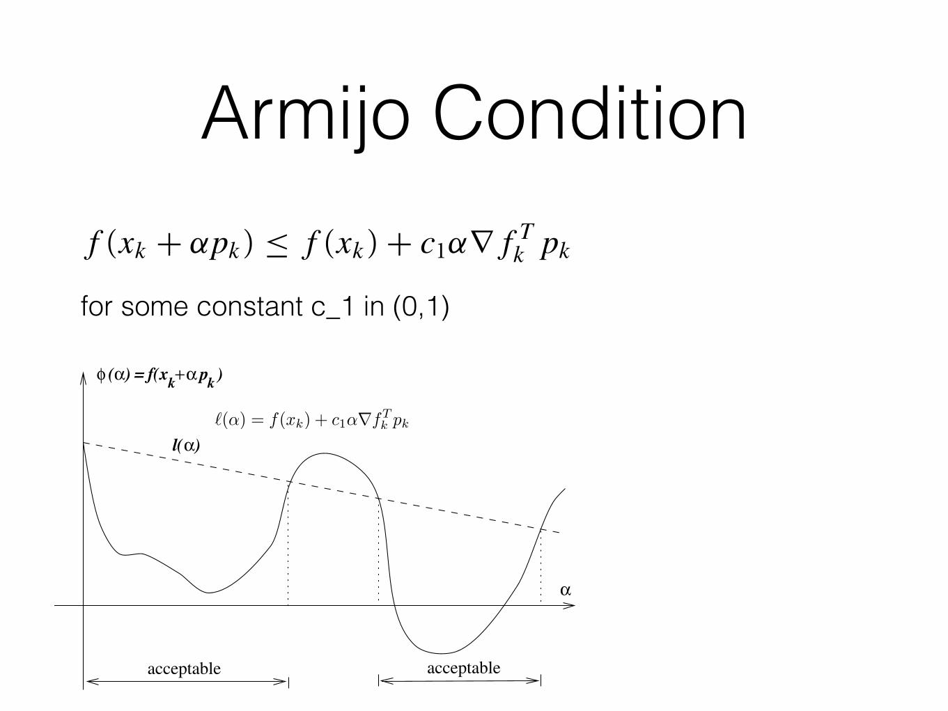
Armijo Condition
3 . 1 . S t e p L e n g t h 37
2x
0x1x
x
xf( )
Figure 3.2 Insufficient reduction in f .
tive function f and possibly the gradient ∇f . More practical strategies perform an inexactline search to identify a step length that achieves adequate reductions in f at minimal cost.
Typical line search algorithms try out a sequence of candidate values for α, stopping toaccept one of these values when certain conditions are satisfied. The line search is done in twostages: A bracketing phase finds an interval containing desirable step lengths, and a bisectionor interpolation phase computes a good step length within this interval. Sophisticated linesearch algorithms can be quite complicated, so we defer a full description until the end ofthis chapter. We now discuss various termination conditions for the line search algorithmand show that effective step lengths need not lie near minimizers of the univariate functionφ(α) defined in (3.3).
A simple condition we could impose on αk is that it provide a reduction in f , i.e.,f (xk + αkpk) < f (xk). That this is not appropriate is illustrated in Figure 3.2, where theminimum is f ∗ # −1, but the sequence of function values {5/k}, k # 0, 1, . . ., convergesto zero. The difficulty is that we do not have sufficient reduction in f , a concept we discussnext.
THE WOLFE CONDITIONS
A popular inexact line search condition stipulates thatαk should first of all give sufficientdecrease in the objective function f , as measured by the following inequality:
f (xk + αpk) ≤ f (xk) + c1α∇f Tk pk, (3.4)
for some constant c_1 in (0,1)38 C h a p t e r 3 . L i n e S e a r c h M e t h o d s
αl( )
φ (α f(x +) = kαk p )
acceptableacceptable
α
Figure 3.3 Sufficient decrease condition.
for some constant c1 ∈ (0, 1). In other words, the reduction in f should be proportional toboth the step length αk and the directional derivative ∇f T
k pk . Inequality (3.4) is sometimescalled the Armijo condition.
The sufficient decrease condition is illustrated in Figure 3.3. The right-hand-side of(3.4), which is a linear function, can be denoted by l(α). The function l(·) has negative slopec1∇f T
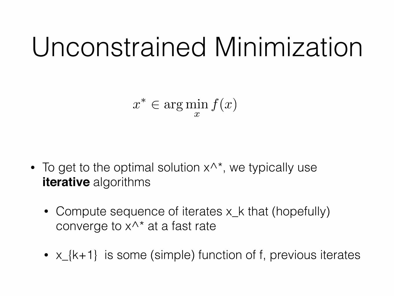
k pk , but because c1 ∈ (0, 1), it lies above the graph of φ for small positive values ofα. The sufficient decrease condition states that α is acceptable only if φ(α) ≤ l(α). Theintervals on which this condition is satisfied are shown in Figure 3.3. In practice, c1 is chosento be quite small, say c1 $ 10−4.
The sufficient decrease condition is not enough by itself to ensure that the algorithmmakes reasonable progress, because as we see from Figure 3.3, it is satisfied for all sufficientlysmall values of α. To rule out unacceptably short steps we introduce a second requirement,called the curvature condition, which requires αk to satisfy
∇f (xk + αkpk)T pk ≥ c2∇f Tk pk, (3.5)
for some constant c2 ∈ (c1, 1), where c1 is the constant from (3.4). Note that the left-hand-side is simply the derivative φ′(αk), so the curvature condition ensures that the slope ofφ(αk) is greater than c2 times the gradient φ′(0). This makes sense because if the slope φ′(α)is strongly negative, we have an indication that we can reduce f significantly by movingfurther along the chosen direction. On the other hand, if the slope is only slightly negativeor even positive, it is a sign that we cannot expect much more decrease in f in this direction,
`(↵) = f(xk) + c1↵rf
Tk pk
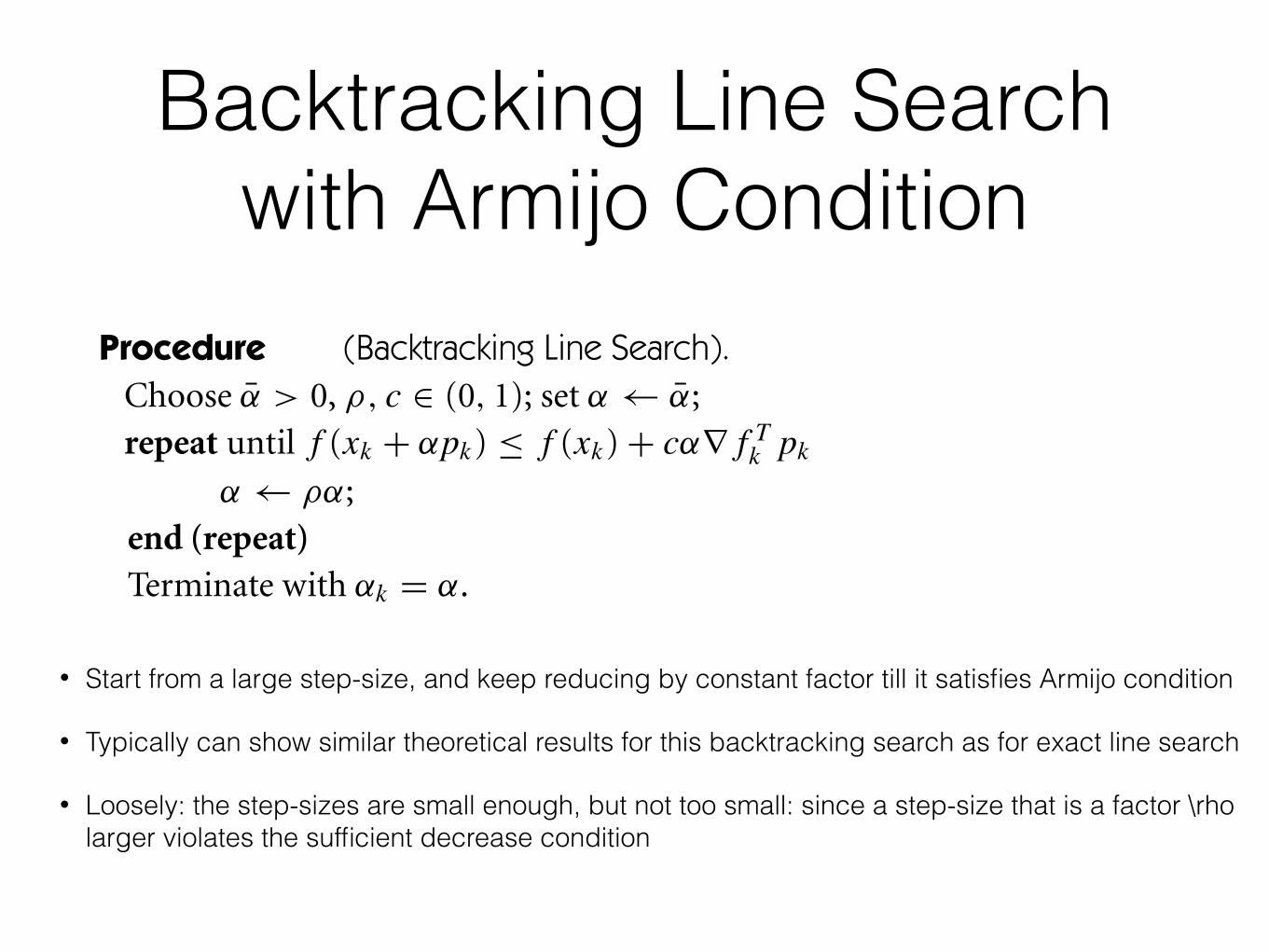
Backtracking Line Search with Armijo Condition
• Start from a large step-size, and keep reducing by constant factor till it satisfies Armijo condition
• Typically can show similar theoretical results for this backtracking search as for exact line search
• Loosely: the step-sizes are small enough, but not too small: since a step-size that is a factor \rho larger violates the sufficient decrease condition
3 . 1 . S t e p L e n g t h 41
By combining (3.8) and (3.9), we obtain
∇f (xk + α′′pk)T pk # c1∇f Tk pk > c2∇f T
k pk, (3.10)
since c1 < c2 and ∇f Tk pk < 0. Therefore, α′′ satisfies the Wolfe conditions (3.6), and the
inequalities hold strictly in both (3.6a) and (3.6b). Hence, by our smoothness assumptionon f , there is an interval around α′′ for which the Wolfe conditions hold. Moreover, sincethe term in the left-hand side of (3.10) is negative, the strong Wolfe conditions (3.7) hold inthe same interval. !
The Wolfe conditions are scale-invariant in a broad sense: Multiplying the objectivefunction by a constant or making an affine change of variables does not alter them. They canbe used in most line search methods, and are particularly important in the implementationof quasi-Newton methods, as we see in Chapter 8.
THE GOLDSTEIN CONDITIONS
Like the Wolfe conditions, the Goldstein conditions also ensure that the step lengthα achieves sufficient decrease while preventing α from being too small. The Goldsteinconditions can also be stated as a pair of inequalities, in the following way:
f (xk) + (1− c)αk∇f Tk pk ≤ f (xk + αkpk) ≤ f (xk) + cαk∇f T
k pk, (3.11)
with 0 < c < 12 . The second inequality is the sufficient decrease condition (3.4), whereas
the first inequality is introduced to control the step length from below; see Figure 3.6A disadvantage of the Goldstein conditions vis-a-vis the Wolfe conditions is that the
first inequality in (3.11) may exclude all minimizers of φ. However, the Goldstein and Wolfeconditions have much in common, and their convergence theories are quite similar. TheGoldstein conditions are often used in Newton-type methods but are not well suited forquasi-Newton methods that maintain a positive definite Hessian approximation.
SUFFICIENT DECREASE AND BACKTRACKING
We have mentioned that the sufficient decrease condition (3.6a) alone is not sufficientto ensure that the algorithm makes reasonable progress along the given search direction.However, if the line search algorithm chooses its candidate step lengths appropriately, byusing a so-called backtracking approach, we can dispense with the extra condition (3.6b) anduse just the sufficient decrease condition to terminate the line search procedure. In its mostbasic form, backtracking proceeds as follows.
Procedure 3.1 (Backtracking Line Search).Choose α > 0, ρ, c ∈ (0, 1); set α← α;repeat until f (xk + αpk) ≤ f (xk) + cα∇f T
k pk
42 C h a p t e r 3 . L i n e S e a r c h M e t h o d s
fkTpkcα
Tpkkα (1_ c) f
φ ( = f(x k+α pα ) k )
acceptable steplengths
α
Figure 3.6 The Goldstein conditions.
α← ρα;end (repeat)Terminate with αk " α.
In this procedure, the initial step length α is chosen to be 1 in Newton and quasi-Newtonmethods, but can have different values in other algorithms such as steepest descent or conju-gate gradient. An acceptable step length will be found after a finite number of trials becauseαk will eventually become small enough that the sufficient decrease condition holds (see Fig-ure 3.3). In practice, the contraction factor ρ is often allowed to vary at each iteration of theline search. For example, it can be chosen by safeguarded interpolation, as we describe later.We need ensure only that at each iteration we have ρ ∈ [ρlo, ρhi], for some fixed constants0 < ρlo < ρhi < 1.
The backtracking approach ensures either that the selected step length αk is somefixed value (the initial choice α), or else that it is short enough to satisfy the sufficientdecrease condition but not too short. The latter claim holds because the accepted value αk
is within striking distance of the previous trial value, αk/ρ, which was rejected for violatingthe sufficient decrease condition, that is, for being too long.
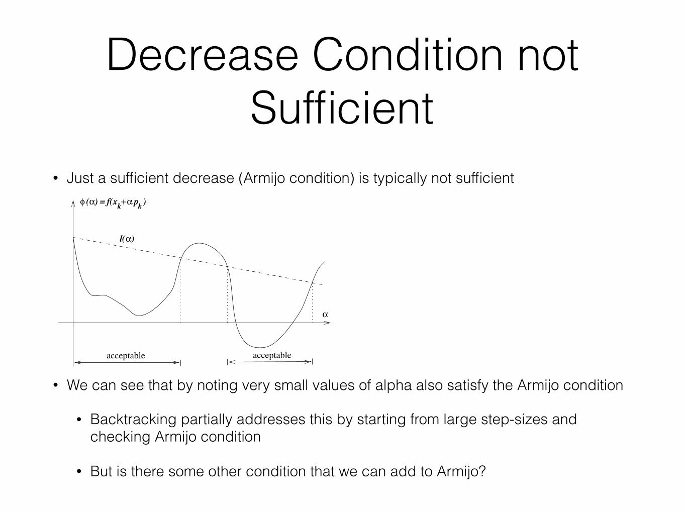
Decrease Condition not Sufficient
• Just a sufficient decrease (Armijo condition) is typically not sufficient
• We can see that by noting very small values of alpha also satisfy the Armijo condition
• Backtracking partially addresses this by starting from large step-sizes and checking Armijo condition
• But is there some other condition that we can add to Armijo?
38 C h a p t e r 3 . L i n e S e a r c h M e t h o d s
αl( )
φ (α f(x +) = kαk p )
acceptableacceptable
α
Figure 3.3 Sufficient decrease condition.
for some constant c1 ∈ (0, 1). In other words, the reduction in f should be proportional toboth the step length αk and the directional derivative ∇f T
k pk . Inequality (3.4) is sometimescalled the Armijo condition.
The sufficient decrease condition is illustrated in Figure 3.3. The right-hand-side of(3.4), which is a linear function, can be denoted by l(α). The function l(·) has negative slopec1∇f T
k pk , but because c1 ∈ (0, 1), it lies above the graph of φ for small positive values ofα. The sufficient decrease condition states that α is acceptable only if φ(α) ≤ l(α). Theintervals on which this condition is satisfied are shown in Figure 3.3. In practice, c1 is chosento be quite small, say c1 $ 10−4.
The sufficient decrease condition is not enough by itself to ensure that the algorithmmakes reasonable progress, because as we see from Figure 3.3, it is satisfied for all sufficientlysmall values of α. To rule out unacceptably short steps we introduce a second requirement,called the curvature condition, which requires αk to satisfy
∇f (xk + αkpk)T pk ≥ c2∇f Tk pk, (3.5)
for some constant c2 ∈ (c1, 1), where c1 is the constant from (3.4). Note that the left-hand-side is simply the derivative φ′(αk), so the curvature condition ensures that the slope ofφ(αk) is greater than c2 times the gradient φ′(0). This makes sense because if the slope φ′(α)is strongly negative, we have an indication that we can reduce f significantly by movingfurther along the chosen direction. On the other hand, if the slope is only slightly negativeor even positive, it is a sign that we cannot expect much more decrease in f in this direction,
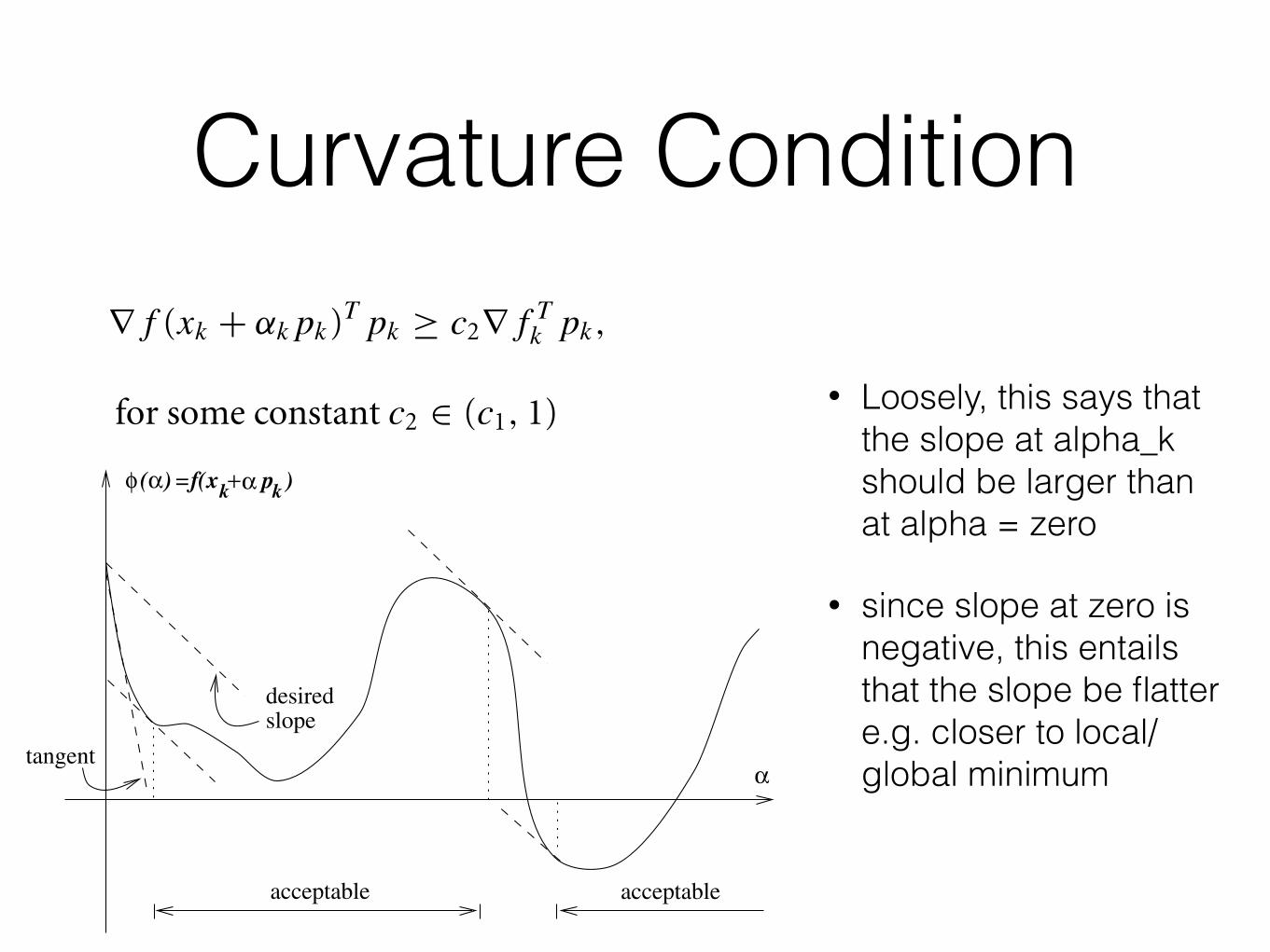
Curvature Condition
• Loosely, this says that the slope at alpha_k should be larger than at alpha = zero
• since slope at zero is negative, this entails that the slope be flatter e.g. closer to local/global minimum
38 C h a p t e r 3 . L i n e S e a r c h M e t h o d s
αl( )
φ (α f(x +) = kαk p )
acceptableacceptable
α
Figure 3.3 Sufficient decrease condition.
for some constant c1 ∈ (0, 1). In other words, the reduction in f should be proportional toboth the step length αk and the directional derivative ∇f T
k pk . Inequality (3.4) is sometimescalled the Armijo condition.
The sufficient decrease condition is illustrated in Figure 3.3. The right-hand-side of(3.4), which is a linear function, can be denoted by l(α). The function l(·) has negative slopec1∇f T
k pk , but because c1 ∈ (0, 1), it lies above the graph of φ for small positive values ofα. The sufficient decrease condition states that α is acceptable only if φ(α) ≤ l(α). Theintervals on which this condition is satisfied are shown in Figure 3.3. In practice, c1 is chosento be quite small, say c1 $ 10−4.
The sufficient decrease condition is not enough by itself to ensure that the algorithmmakes reasonable progress, because as we see from Figure 3.3, it is satisfied for all sufficientlysmall values of α. To rule out unacceptably short steps we introduce a second requirement,called the curvature condition, which requires αk to satisfy
∇f (xk + αkpk)T pk ≥ c2∇f Tk pk, (3.5)
for some constant c2 ∈ (c1, 1), where c1 is the constant from (3.4). Note that the left-hand-side is simply the derivative φ′(αk), so the curvature condition ensures that the slope ofφ(αk) is greater than c2 times the gradient φ′(0). This makes sense because if the slope φ′(α)is strongly negative, we have an indication that we can reduce f significantly by movingfurther along the chosen direction. On the other hand, if the slope is only slightly negativeor even positive, it is a sign that we cannot expect much more decrease in f in this direction,
3 . 1 . S t e p L e n g t h 39
desiredslope
k )φ (α)=f(xk+α p
tangentα
acceptableacceptable
Figure 3.4 The curvature condition.
so it might make sense to terminate the line search. The curvature condition is illustrated inFigure 3.4. Typical values of c2 are 0.9 when the search direction pk is chosen by a Newtonor quasi-Newton method, and 0.1 when pk is obtained from a nonlinear conjugate gradientmethod.
The sufficient decrease and curvature conditions are known collectively as the Wolfeconditions. We illustrate them in Figure 3.5 and restate them here for future reference:
f (xk + αkpk) ≤ f (xk) + c1αk∇f Tk pk, (3.6a)
∇f (xk + αkpk)T pk ≥ c2∇f Tk pk, (3.6b)
with 0 < c1 < c2 < 1.A step length may satisfy the Wolfe conditions without being particularly close to a
minimizer of φ, as we show in Figure 3.5. We can, however, modify the curvature conditionto force αk to lie in at least a broad neighborhood of a local minimizer or stationary pointof φ. The strong Wolfe conditions require αk to satisfy
f (xk + αkpk) ≤ f (xk) + c1αk∇f Tk pk, (3.7a)
|∇f (xk + αkpk)T pk| ≤ c2|∇f Tk pk|, (3.7b)
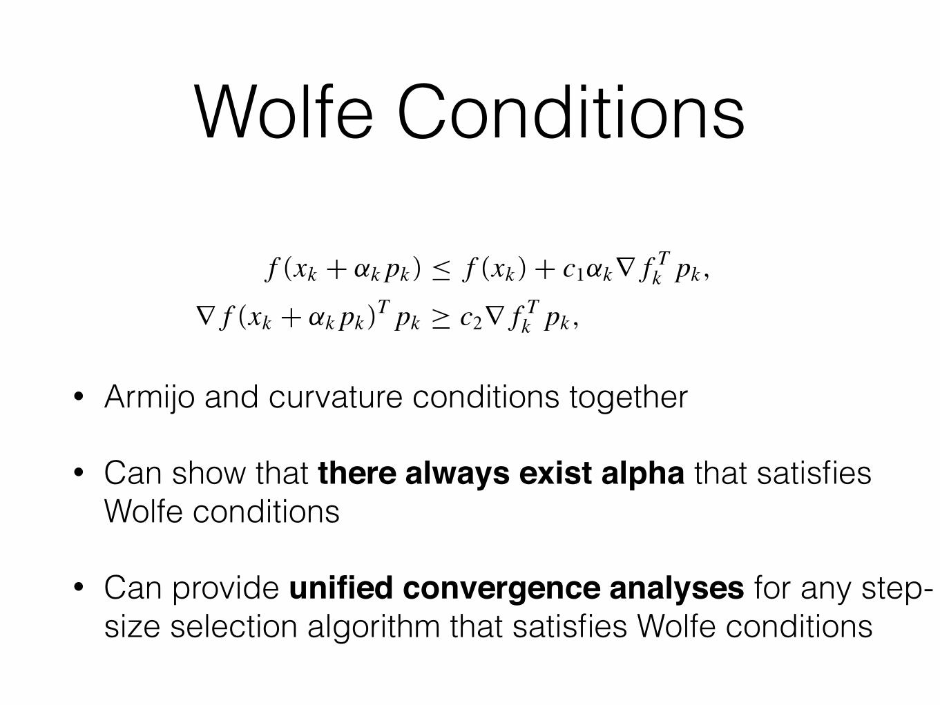
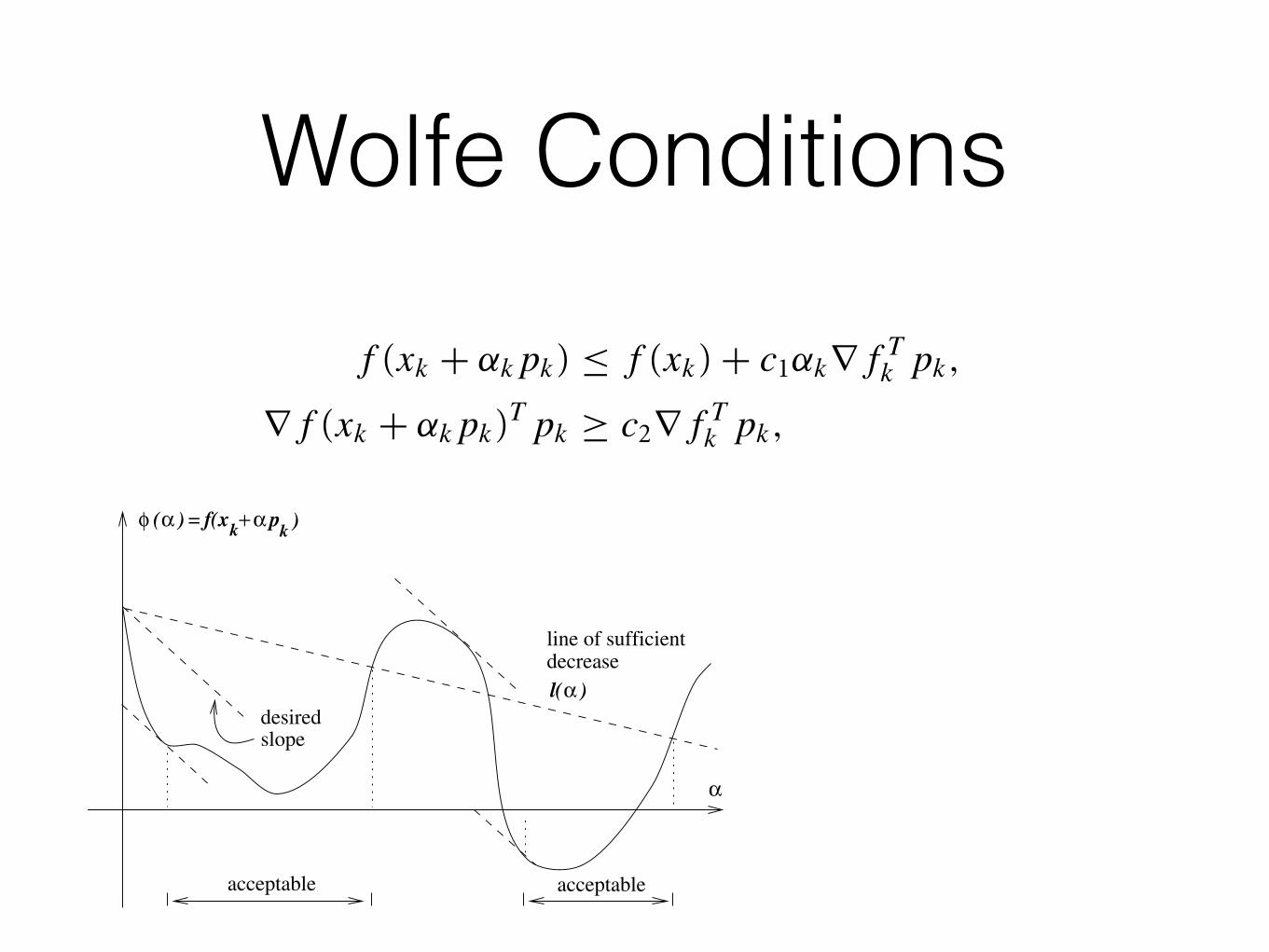
Wolfe Conditions
• Armijo and curvature conditions together
• Can show that there always exist alpha that satisfies Wolfe conditions
• Can provide unified convergence analyses for any step-size selection algorithm that satisfies Wolfe conditions
3 . 1 . S t e p L e n g t h 39
desiredslope
k )φ (α)=f(xk+α p
tangentα
acceptableacceptable
Figure 3.4 The curvature condition.
so it might make sense to terminate the line search. The curvature condition is illustrated inFigure 3.4. Typical values of c2 are 0.9 when the search direction pk is chosen by a Newtonor quasi-Newton method, and 0.1 when pk is obtained from a nonlinear conjugate gradientmethod.
The sufficient decrease and curvature conditions are known collectively as the Wolfeconditions. We illustrate them in Figure 3.5 and restate them here for future reference:
f (xk + αkpk) ≤ f (xk) + c1αk∇f Tk pk, (3.6a)
∇f (xk + αkpk)T pk ≥ c2∇f Tk pk, (3.6b)
with 0 < c1 < c2 < 1.A step length may satisfy the Wolfe conditions without being particularly close to a
minimizer of φ, as we show in Figure 3.5. We can, however, modify the curvature conditionto force αk to lie in at least a broad neighborhood of a local minimizer or stationary pointof φ. The strong Wolfe conditions require αk to satisfy
f (xk + αkpk) ≤ f (xk) + c1αk∇f Tk pk, (3.7a)
|∇f (xk + αkpk)T pk| ≤ c2|∇f Tk pk|, (3.7b)
Wolfe Conditions
3 . 1 . S t e p L e n g t h 39
desiredslope
k )φ (α)=f(xk+α p
tangentα
acceptableacceptable
Figure 3.4 The curvature condition.
so it might make sense to terminate the line search. The curvature condition is illustrated inFigure 3.4. Typical values of c2 are 0.9 when the search direction pk is chosen by a Newtonor quasi-Newton method, and 0.1 when pk is obtained from a nonlinear conjugate gradientmethod.
The sufficient decrease and curvature conditions are known collectively as the Wolfeconditions. We illustrate them in Figure 3.5 and restate them here for future reference:
f (xk + αkpk) ≤ f (xk) + c1αk∇f Tk pk, (3.6a)
∇f (xk + αkpk)T pk ≥ c2∇f Tk pk, (3.6b)
with 0 < c1 < c2 < 1.A step length may satisfy the Wolfe conditions without being particularly close to a
minimizer of φ, as we show in Figure 3.5. We can, however, modify the curvature conditionto force αk to lie in at least a broad neighborhood of a local minimizer or stationary pointof φ. The strong Wolfe conditions require αk to satisfy
f (xk + αkpk) ≤ f (xk) + c1αk∇f Tk pk, (3.7a)
|∇f (xk + αkpk)T pk| ≤ c2|∇f Tk pk|, (3.7b)
40 C h a p t e r 3 . L i n e S e a r c h M e t h o d s
slopedesired
line of sufficientdecreasel(α )
acceptable
α
φ (α )= αpf(x + kk )
acceptable
Figure 3.5 Step lengths satisfying the Wolfe conditions.
with 0 < c1 < c2 < 1. The only difference with the Wolfe conditions is that we no longerallow the derivative φ′(αk) to be too positive. Hence, we exclude points that are far fromstationary points of φ.
It is not difficult to prove that there exist step lengths that satisfy the Wolfe conditionsfor every function f that is smooth and bounded below.
Lemma 3.1.Suppose that f : IRn → IR is continuously differentiable. Let pk be a descent direction at
xk , and assume that f is bounded below along the ray {xk + αpk|α > 0}. Then if 0 < c1 <
c2 < 1, there exist intervals of step lengths satisfying the Wolfe conditions (3.6) and the strongWolfe conditions (3.7).
Proof. Since φ(α) # f (xk + αpk) is bounded below for all α > 0 and since 0 < c1 < 1,the line l(α) # f (xk) + αc1∇f T
k pk must intersect the graph of φ at least once. Let α′ > 0be the smallest intersecting value of α, that is,
f (xk + α′pk) # f (xk) + α′c1∇f Tk pk. (3.8)
The sufficient decrease condition (3.6a) clearly holds for all step lengths less than α′.By the mean value theorem, there exists α′′ ∈ (0,α′) such that
f (xk + α′pk)− f (xk) # α′∇f (xk + α′′pk)T pk. (3.9)
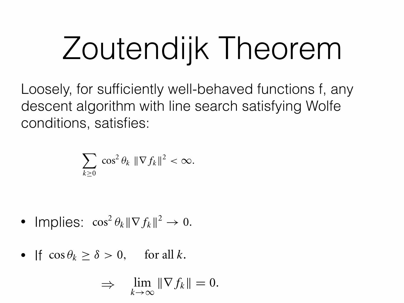
Zoutendijk Theorem
• Implies:
• If
44 C h a p t e r 3 . L i n e S e a r c h M e t h o d s
while the Lipschitz condition (3.13) implies that
(∇fk+1 − ∇fk)T pk ≤ αkL∥pk∥2.
By combining these two relations, we obtain
αk ≥c2 − 1
L
∇f Tk pk
∥pk∥2.
By substituting this inequality into the first Wolfe condition (3.6a), we obtain
fk+1 ≤ fk − c11− c2
L
(∇f Tk pk)2
∥pk∥2.
From the definition (3.12), we can write this relation as
fk+1 ≤ fk − c cos2 θk∥∇fk∥2,
where c & c1(1 − c2)/L. By summing this expression over all indices less than or equal tok, we obtain
fk+1 ≤ f0 − ck!
j&0
cos2 θj∥∇fj∥2. (3.15)
Since f is bounded below, we have that f0− fk+1 is less than some positive constant, for allk. Hence by taking limits in (3.15), we obtain
∞!
k&0
cos2 θk∥∇fk∥2 <∞,
which concludes the proof. !
Similar results to this theorem hold when the Goldstein conditions (3.11) or strongWolfe conditions (3.7) are used in place of the Wolfe conditions.
Note that the assumptions of Theorem 3.2 are not too restrictive. If the function f werenot bounded below, the optimization problem would not be well-defined. The smoothnessassumption—Lipschitz continuity of the gradient—is implied by many of the smoothnessconditions that are used in local convergence theorems (see Chapters 6 and 8) and are oftensatisfied in practice.
Inequality (3.14), which we call the Zoutendijk condition, implies that
cos2 θk∥∇fk∥2 → 0. (3.16)
3 . 2 . C o n v e r g e n c e o f L i n e S e a r c h M e t h o d s 45
This limit can be used in turn to derive global convergence results for line search algorithms.If our method for choosing the search direction pk in the iteration (3.1) ensures that
the angle θk defined by (3.12) is bounded away from 90◦, there is a positive constant δ suchthat
cos θk ≥ δ > 0, for all k. (3.17)
It follows immediately from (3.16) that
limk→∞∥∇fk∥ ' 0. (3.18)
In other words, we can be sure that the gradient norms∥∇fk∥ converge to zero, provided thatthe search directions are never too close to orthogonality with the gradient. In particular, themethod of steepest descent (for which the search direction pk makes an angle of zero degreeswith the negative gradient) produces a gradient sequence that converges to zero, providedthat it uses a line search satisfying the Wolfe or Goldstein conditions.
We use the term globally convergent to refer to algorithms for which the property(3.18) is satisfied, but note that this term is sometimes used in other contexts to meandifferent things. For line search methods of the general form (3.1), the limit (3.18) is thestrongest global convergence result that can be obtained: We cannot guarantee that themethod converges to a minimizer, but only that it is attracted by stationary points. Onlyby making additional requirements on the search direction pk—by introducing negativecurvature information from the Hessian ∇2f (xk), for example—can we strengthen theseresults to include convergence to a local minimum. See the Notes and References at the endof this chapter for further discussion of this point.
Consider now the Newton-like method (3.1), (3.2) and assume that the matrices Bk
are positive definite with a uniformly bounded condition number. That is, there is a constantM such that
∥Bk∥ ∥B−1k ∥ ≤ M, for all k.
It is easy to show from the definition (3.12) that
cos θk ≥ 1/M (3.19)
(see Exercise 5). By combining this bound with (3.16) we find that
limk→∞∥∇fk∥ ' 0. (3.20)
Therefore, we have shown that Newton and quasi-Newton methods are globally convergentif the matrices Bk have a bounded condition number and are positive definite (which is
)
Loosely, for sufficiently well-behaved functions f, any descent algorithm with line search satisfying Wolfe conditions, satisfies:
3 . 2 . C o n v e r g e n c e o f L i n e S e a r c h M e t h o d s 43
This simple and popular strategy for terminating a line search is well suited for Newtonmethods (see Chapter 6) but is less appropriate for quasi-Newton and conjugate gradientmethods.
3.2 CONVERGENCE OF LINE SEARCH METHODS
To obtain global convergence, we must not only have well-chosen step lengths but also well-chosen search directions pk . We discuss requirements on the search direction in this section,focusing on one key property: the angle θk between pk and the steepest descent direction−∇fk , defined by
cos θk #−∇f T
k pk
∥∇fk∥ ∥pk∥. (3.12)
The following theorem, due to Zoutendijk, has far-reaching consequences. It shows,for example, that the steepest descent method is globally convergent. For other algorithmsit describes how far pk can deviate from the steepest descent direction and still give rise toa globally convergent iteration. Various line search termination conditions can be used toestablish this result, but for concreteness we will consider only the Wolfe conditions (3.6).Though Zoutendijk’s result appears, at first, to be technical and obscure, its power will soonbecome evident.
Theorem 3.2.Consider any iteration of the form (3.1), where pk is a descent direction and αk satisfies
the Wolfe conditions (3.6). Suppose that f is bounded below in IRn and that f is continuously
differentiable in an open set N containing the level set L def# {x : f (x) ≤ f (x0)}, where x0 isthe starting point of the iteration. Assume also that the gradient ∇f is Lipschitz continuous onN , that is, there exists a constant L > 0 such that
∥∇f (x)− ∇f (x)∥ ≤ L∥x − x∥, for all x, x ∈ N . (3.13)
Then
!
k≥0
cos2 θk ∥∇fk∥2 <∞. (3.14)
Proof. From (3.6b) and (3.1) we have that
(∇fk+1 − ∇fk)T pk ≥ (c2 − 1)∇f Tk pk,
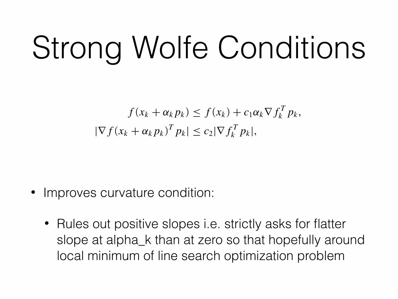
Strong Wolfe Conditions
• Improves curvature condition:
• Rules out positive slopes i.e. strictly asks for flatter slope at alpha_k than at zero so that hopefully around local minimum of line search optimization problem
3 . 1 . S t e p L e n g t h 39
desiredslope
k )φ (α)=f(xk+α p
tangentα
acceptableacceptable
Figure 3.4 The curvature condition.
so it might make sense to terminate the line search. The curvature condition is illustrated inFigure 3.4. Typical values of c2 are 0.9 when the search direction pk is chosen by a Newtonor quasi-Newton method, and 0.1 when pk is obtained from a nonlinear conjugate gradientmethod.
The sufficient decrease and curvature conditions are known collectively as the Wolfeconditions. We illustrate them in Figure 3.5 and restate them here for future reference:
f (xk + αkpk) ≤ f (xk) + c1αk∇f Tk pk, (3.6a)
∇f (xk + αkpk)T pk ≥ c2∇f Tk pk, (3.6b)
with 0 < c1 < c2 < 1.A step length may satisfy the Wolfe conditions without being particularly close to a
minimizer of φ, as we show in Figure 3.5. We can, however, modify the curvature conditionto force αk to lie in at least a broad neighborhood of a local minimizer or stationary pointof φ. The strong Wolfe conditions require αk to satisfy
f (xk + αkpk) ≤ f (xk) + c1αk∇f Tk pk, (3.7a)
|∇f (xk + αkpk)T pk| ≤ c2|∇f Tk pk|, (3.7b)
(Strong) Wolfe Condition Algorithms
• Armijo condition ensures sufficient decrease
• Curvature condition ensures that step-size is not too small (otherwise won’t make enough progress)
• Backtracking algorithm introduced earlier finesses need for curvature condition by starting from large step-size and iteratively reducing step-size
• not guaranteed to satisfy Wolfe conditions per se
• Algorithms targeted to satisfying Wolfe conditions tricky to code, even trickier to analyze