Embed Size (px)
Citation preview
Under consideration for publication in Theory and Practice of Logic Programming 1
Description and Optimization of AbstractMachines in a Dialect of Prolog∗
JOSE F. MORALES1 MANUEL CARRO1,2 MANUEL HERMENEGILDO1,2
1 IMDEA Software Institute
(e-mail: {josef.morales,manuel.carro,manuel.hermenegildo}@imdea.org)2 School of Computer Science, Technical University of Madrid (UPM)
(e-mail: {mcarro,herme}@fi.upm.es)
submitted 26 January 2007; revised 8 July 2009, 20 April 2014; accepted 26 June 2014
Note: To appear in Theory and Practice of Logic Programming (TPLP)
Abstract
In order to achieve competitive performance, abstract machines for Prolog and relatedlanguages end up being large and intricate, and incorporate sophisticated optimizations,both at the design and at the implementation levels. At the same time, efficiency consid-erations make it necessary to use low-level languages in their implementation. This makesthem laborious to code, optimize, and, especially, maintain and extend. Writing the ab-stract machine (and ancillary code) in a higher-level language can help tame this inherentcomplexity. We show how the semantics of most basic components of an efficient virtualmachine for Prolog can be described using (a variant of) Prolog. These descriptions arethen compiled to C and assembled to build a complete bytecode emulator. Thanks to thehigh level of the language used and its closeness to Prolog, the abstract machine descrip-tion can be manipulated using standard Prolog compilation and optimization techniqueswith relative ease. We also show how, by applying program transformations selectively, weobtain abstract machine implementations whose performance can match and even exceedthat of state-of-the-art, highly-tuned, hand-crafted emulators.
KEYWORDS: Abstract Machines, Compilation, Optimization, Program Transformation,Prolog, Logic Languages.
1 Introduction
Abstract machines have proved themselves very useful when defining theoretical
models and implementations of software and hardware systems. In particular, they
have been widely used to define execution models and as implementation vehi-
cles for many languages, most frequently in functional and logic programming, and
∗ This is a significantly extended and revised version of the paper “Towards Description andOptimization of Abstract Machines in an Extension of Prolog” published in the proceedingsof the 2006 International Symposium on Logic-based Program Synthesis and Transformation(LOPSTR’06) (Morales et al. 2007).
arX
iv:1
411.
5573
v1 [
cs.P
L]
20
Nov
201
4

2 J. F. Morales, M. Carro, and M. Hermenegildo
more recently also in object-oriented programming, with the Java abstract ma-
chine (Gosling et al. 2005) being a very popular recent example. There are also
early examples of the use of abstract machines in traditional procedural languages
(e.g., the P-Code used as a target in early Pascal implementations (Nori et al.
1981)) and in other realms such as, for example, operating systems (e.g., Dis, the
virtual machine for the Inferno operating system (Dorward et al. 1997)).
The practical applications of the indirect execution mechanism that an abstract
machine represents are countless: portability, generally small executables, simpler
security control through sandboxing, increased compilation speed, etc. However,
unless the abstract machine implementation is highly optimized, these benefits can
come at the cost of poor performance. Designing and implementing fast, resource-
friendly, competitive abstract machines is a complex task. This is especially so in
the case of programming languages where there is a wide gap between many of their
basic constructs and features and what is available in the underlying off-the-shelf
hardware: term representation vs. memory words, unification vs. assignment, au-
tomatic vs. manual memory management, destructive vs. non-destructive updates,
backtracking and tabling vs. Von Neumann-style control flow, etc. In addition, the
extensive code optimizations required to achieve good performance make devel-
opment and, especially, maintenance and further modifications non-trivial. Imple-
menting or testing new optimizations is often involved, as decisions previously taken
need to be revisited, and low-level, tedious recoding is often necessary to test a new
idea.
Improved performance has been achieved by post-processing the input program
(often called bytecode) of the abstract machine (emulator) and generating efficient
native code — sometimes achieving performance that is very close to that of an
implementation of the source program directly written in C. This is technically
challenging and the overall picture is even more complex when bytecode and native
code are mixed, usually by dynamic recompilation. This in principle combines the
best of both worlds by deciding when and how native code (which may be large
and/or costly to obtain) is generated based on runtime analysis of the program
execution, while leaving the rest as bytecode. Some examples are the Java HotSpot
VM (Paleczny et al. 2001), the Psyco (Rigo 2004) extension for Python, or for
logic programming, all-argument predicate indexing in recent versions of Yap Pro-
log (Santos-Costa et al. 2007), the dynamic recompilation of asserted predicates
in BinProlog (Tarau 2006), etc. Note, however, that the initial complexity of the
virtual machine and all of its associated maintenance issues have not disappeared,
and emulator designers and maintainers still have to struggle with thousands of
lines of low-level code.
In this paper we explore the possibility of rewriting most of the runtime and vir-
tual machine in the high-level source language (or a close dialect of it), and then use
all the available compilation machinery to obtain native code from it. Ideally, this
native code should provide comparable performance to that of hand-crafted code,
while keeping the size of low-level coded parts in the system to a minimum. This is
the approach taken herein, where we explore writing Prolog emulators in a Prolog
dialect. As we will see later, the approach is interesting not only for simplifying the

Theory and Practice of Logic Programming 3
task of developers but also for widening the application domain of the language
to other kinds of problems which extend beyond just emulators, such as reusing
analysis and transformation passes, and making it easier to automate tedious opti-
mization techniques for emulators, such as specializing emulator instructions. The
advantages of using a higher-level language are rooted on one hand in the capability
of hiding implementation details that a higher-level language provides, and on the
other hand in its amenability to transformation and manipulation. These, as we will
see, are key for our goals, as they reduce error-prone, tedious programming work,
while making it possible to describe at the same time complex abstract machines
in a concise and correct way.
A similar objective has been pursued elsewhere. For example, the JavaInJava (Taival-
saari 1998) and PyPy (Rigo and Pedroni 2006) projects have similar goals. The
initial performance figures reported for these implementations highlight how chal-
lenging it is to make them competitive with existing hand-tuned abstract machines:
JavaInJava started with an initial slowdown of approximately 700 times w.r.t. then-
current implementations, and PyPy started at the 2000× slowdown level. Compet-
itive execution times were only possible after changes in the source language and
compilation tool chain, by restricting it or adding annotations. For example, the
slowdown of PyPy was reduced to 3.5× – 11.0× w.r.t. CPython (Rigo and Pedroni
2006). These results can be partially traced back to the attempt to reimplement the
whole machinery at once, which has the disadvantage of making such a slowdown
almost inevitable. This makes it difficult to use the generated virtual machines as
“production” software (which would therefore be routinely tested) and, especially,
it makes it difficult to study how a certain, non-local optimization will carry over
to a complete, optimized abstract machine.
Therefore, we chose an alternative approach: gradually porting selected key com-
ponents (such as, e.g., instruction definitions) and combining this port with other
emulator generation techniques (Morales et al. 2005). At every step we made sure
experimentally1 that the performance of the original emulator was maintained
throughout the process. The final result is an emulator that is completely writ-
ten in a high-level language and which, when compiled to native code, does not
lose any performance w.r.t. a manually written emulator. Also, and as a very rele-
vant byproduct, we develop a language (and a compiler for it) which is high-level
enough to make several program transformation and analysis techniques applica-
ble, while offering the possibility of being compiled into efficient native code. While
this language is general-purpose and can be used to implement arbitrary programs,
throughout this paper we will focus on its use in writing abstract machines and to
easily generate variations of such machines.
The rest of the paper proceeds as follows: Section 2 gives an overview of the differ-
ent parts of our compilation architecture and information flow and compares it with
a more traditional setup. Section 3 presents the source language with which our ab-
1 And also with stronger means: for some core components we checked that the binary codeproduced from the high-level definition of the abstract machine and that coming from thehand-written one were identical.

4 J. F. Morales, M. Carro, and M. Hermenegildo
stract machine is written, and justifies the design decisions (e.g., typing, destructive
updates, etc.) based on the needs of applications which demand high performance.
Section 3.4 summarizes how compilation to efficient native code is done through
C. Section 4 describes language extensions which were devised specifically to write
abstract machines (in particular, the WAM) and Section 5 explores how the added
flexibility of the high-level language approach can be taken advantage of in order
to easily generate variants of abstract machines with different core characteristics.
This section also studies experimentally the performance that can be attained with
these variants. Finally, Section 6 presents our conclusions.
2 Overview of our Compilation Architecture
The compilation architecture we present here uses several languages, language trans-
lators, and program representations which must be defined and placed in the “big
picture.” For generality, and since those elements are common to most bytecode-
based systems, we will refer to them by more abstract names when possible or
convenient, although in our initial discussion we will equate them with the actual
languages in our production environment.
The starting point in this work is the Ciao system (Hermenegildo et al. 2012),
which includes an efficient, WAM-based (Warren 1983; Ait-Kaci 1991), abstract
machine coded in C (an independent evolution which forked from the SICStus
0.5/0.7 virtual machine), a compiler to bytecode with an experimental extension
to emit optimized C code (Morales et al. 2004), and the CiaoPP preprocessor, a
program analysis, specialization and transformation framework (Bueno et al. 1997;
Hermenegildo et al. 1999; Puebla et al. 2000b; Hermenegildo et al. 2005).
We will denote the source Prolog language as Ls, the symbolic WAM code as
La, the byte-encoded WAM code as Lb, and the C language as Lc. The different
languages and translation processes described in this section are typically found in
most Prolog systems, and this scheme could be easily applied to other situations.
We will use N:L to denote the program N written in language L. Thus, we can
distinguish in the traditional approach (Figure 1):
Front-end compiler: P:Ls is compiled to P:Li, where Ls is the source language
and Li is an intermediate representation. For simplicity, we assume that this
phase includes any analysis, transformation, and optimization.
Bytecode back-end: P:Li is translated to P:La, where La is the symbolic repre-
sentation of the bytecode language.
Bytecode assembler: P:La is encoded into P:Lb, where Lb defines encoded byte-
code streams (a sequence of bytes whose design is focused on interpretation
speed).
To execute Lb programs, a hand-written emulator E:Lc (where Lc is a lower-level
language) is required, in addition to some runtime code (written in Lc). Alterna-
tively, it is possible to translate intermediate code by means of a low level back

Theory and Practice of Logic Programming 5
Traditional approach
Lb emulatorE:Lc
low-level code(hand written)
user programP:Ls
source code
Front-endcompiler
P:Li
intermediate code
Bytecodeback-end
P:La
symbolicbytecode
Bytecodeassembler
P:Lb
bytecode
Low-levelback-end
P:Lc
low-level code
Emulation and native compilation must ex-hibit the same behaviour:(E:Lc ◦ P:Lb) ≡ (P:Lc)
Fig. 1. Traditional compilation architecture.
end, which compiles a program P:Li directly into its,P:Lc equivalent.2 This avoids
the need for any emulator if all programs are compiled to native code, but additional
runtime support is usually necessary.
The initial classical architecture needs manual coding of a large and complex piece
of code, the emulator, using a low-level language, often missing the opportunity to
reuse compilation techniques that may have been developed for high-level languages,
not only to improve efficiency, but also program readability, correctness, etc.
In the extended compilation scheme we assume that we can design a dialect from
Ls and write the emulator for symbolic La code, instead of byte-encoded Lb, in
that language. We will call Lrs the extended language and Er:Lr
s the emulator. Note
that the mechanical generation of an interpreter for Lb from an interpreter for La
was previously described and successfully tested in an emulator generator (Morales
et al. 2005). Adopting it for this work was perceived as a correct decision, since it
moves low-level implementation (and bytecode representation) issues to a transla-
tion phase, thus reducing the requirements on the language to preserve emulator
efficiency, and in practice making the code easier to manage. The new translation
pipeline, depicted in the extended approach path (Figure 2) shows the following
2 Note that in JIT systems the low-level code is generated from the encoded bytecode represen-tation. For simplicity we keep the figure for static code generation, which takes elements of Lias the input.
6 J. F. Morales, M. Carro, and M. Hermenegildo
Extended approach
user programP:Ls
source code
Front-endcompiler
P:Li
intermediate code
Bytecodeback-end
P:La
symbolicbytecode
Bytecodeassembler
P:Lb
bytecode
Low-levelback-end
P:Lc
low-level code
La emulatorEr:Lr
s
source code
Lb emulatorEr:Lr
i
intermediate code
Front-endcompiler
Lrs , La;Lb support
Er:Lc
low-level code
Low-levelback-end
Lri support
Emulation and native compilation must ex-hibit the same behaviour:(Er:Lc ◦ P:Lb) ≡ (P:Lc)Generated and hand-written (Figure 1 emu-lators should be equivalent:(Er:Lc ◦ P:Lb) ≡ (E:Lc ◦ P:Lb)
Fig. 2. Extended compilation architecture.
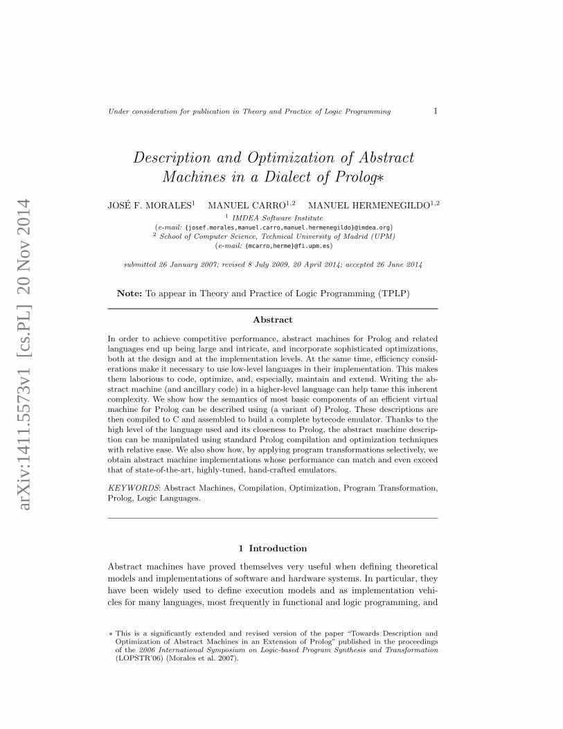
processes (the dashed lines represent the modifications that some of the elements
undergo with respect to the original ones):
Extended front-end compiler: it compiles Lrs programs into Lr
i programs (where
Lri is the intermediate language with extensions required to produce efficient na-
tive code). This compiler includes the emulator generator. That framework makes
it possible to write instruction definitions for an La emulator, plus separate byte-
code encoding rules, and process them together to obtain an Lb emulator. I.e., it
translates Er:Lrs to an Er:Lr
i emulator for Lb.
Extended low-level back-end: it compiles Lri programs into Lc programs. The
resulting Er:Lri is finally translated to Er:Lc, which should be equivalent (in the
sense of producing the same output) to E:Lc.
The advantage of this scheme lies in its flexibility for sharing optimizations, analy-
ses, and transformations at different compilation stages (e.g., the same machinery
for partial evaluation, constant propagation, common subexpression elimination,
etc. can be reused), which are normally reimplemented for high- and low-level lan-
guages.

Theory and Practice of Logic Programming 7
3 The imProlog Language
We describe in this section our Lrs language, imProlog, and the analysis and code
generation techniques used to compile it into highly efficient code.3 This Prolog
variant is motivated by the following problems:
• It is hard to guarantee that certain overheads in Prolog that are directly
related with the language expressiveness (e.g., boxed data for dynamic typing,
trailing for non-determinism, uninstantiated free variables, multiple-precision
arithmetic, etc.) will always be removed by compile-time techniques.
• Even if that overhead could be eliminated, there is also the cost of some basic
operations, such as modifying a single attribute in a custom data structure,
which is not constant in the declarative subset of Prolog. For example, the
cost of replacing the value of an argument in a Prolog structure is, in most
straightforward implementations, linear w.r.t. the number of arguments of the
structure, since a certain amount of copying of the structure spine is typically
involved. In contrast, replacing an element in a C structure is a constant-
time operation. Again, while this overhead can be optimized away in some
cases during compilation, the objective is to define a language layer in which
constant-time can be ensured for these operations.
We now present the different elements that comprise the imProlog language and we
will gradually introduce a number of restrictions on the kind of programs which
we admit as valid. The main reason to impose these restrictions is to achieve the
central goal in this paper: generating efficient emulators starting from a high-level
language.
In a nutshell, the imProlog language both restricts and extends Prolog. The im-
pure features (e.g., the dynamic database) of Prolog are not part of imProlog and
only programs meeting some strict requirements about determinism, modes in the
unification, and others, are allowed. In a somewhat circular fashion, the require-
ments we impose on these programs are those which allow us to compile them into
efficient code. Therefore, implementation matters somewhat influence the design
and semantics of the language. On the other hand, imProlog also extends Prolog in
order to provide a single, well-defined, and amenable to analysis mechanism to im-
plement constant-time access to data: a specific kind of mutable variables. Thanks
to the restrictions aforementioned and this mechanism imProlog programs can be
compiled into very efficient low-level (e.g., C) code.
Since we are starting from Prolog, which is well understood, and the restrictions
on the admissible programs can be introduced painlessly (they just reduce the set
of programs which are deemed valid by the compiler), we will start by showing,
in the next section, how we tackle efficient data handling, which as we mentioned
departs significantly, but in a controlled way, from the semantics of Prolog.
3 The name imProlog stands for imperative Prolog, because its purpose is to make typicallyimperative algorithms easier to express in Prolog, but minimizing and controlling the scope ofimpurities.

8 J. F. Morales, M. Carro, and M. Hermenegildo
Notation. We will use lowercase math font for variables (x, y, z, ...) in the rules
that describe the compilation and language semantics. Prolog variable names will
be written in math capital font (X, Y, Z, ...). Keywords and identifiers in the target
C language use bold text (return). Finally, sans serif text is used for other names
and identifiers (f, g, h, ...). The typography will make it possible to easily distinguish
a compilation pattern for ‘f(a)’, where ‘a’ may be any valid term, and ‘f(A)’, where
‘A’ is a Prolog variable with the concrete name “A.” Similarly, the expression f (a1,
..., an) denotes any structure with functor name f and n arguments, whatever they
may be. It differs from f(A1, ..., An), where the functor name is fixed to f and the
arguments are variables). If n is 0, the previous expression is tantamount to just f.
3.1 Efficient Mechanisms for Data Access and Update
In this section we will describe the formal semantics of typed mutable variables,
our proposal for providing efficient (in terms of time and memory) data handling
in imProlog. These variables feature backtrackable destructive assignment and are
accessible and updatable in constant time through the use of a unique, associated
identifier. This is relevant for us as it is required to efficiently implement a wide
variety of algorithms, some of which appear in WAM-based abstract machines,4
which we want to describe in enough detail as to obtain efficient executables.
There certainly exist a number options for implementing constant-time data ac-
cess in Prolog. Dynamic predicates (assert / retract) can in some cases (maybe with
the help of type information) provide constant-time operations; existing destructive
update primitives (such as setarg/3) can do the same. However, it is difficult for
the analyses normally used in the context of logic programming to deal with them
in a precise way, in a significant part because their semantics was not devised with
analysis in mind, and therefore they are difficult to optimize as much as we need
herein.
Therefore, we opted for a generalization of mutable variables with typing con-
straints as mentioned before. In our experience, this fits in a less intrusive way with
the rest of the logic framework, and at the same time allows us to generate efficient
code for the purpose of the work in this paper.5 Let us introduce some preliminary
definitions before presenting the semantics of mutable variables:
Type: τ is a unary predicate that defines a set of values (e.g., regular types as
in (Dart and Zobel 1992; Gallagher and de Waal 1994; Vaucheret and Bueno
2002)). If τ(v) holds, then v is said to contain values of type τ .
Mutable identifier: the identifier id of a mutable is a unique atomic value that
4 One obvious example is the unification algorithm of logical variables, itself based on the Union-Find algorithm. An interesting discussion of this point is available in (Schrijvers and Fruhwirth2006), where a CHR version of the Union-Find algorithm is implemented and its complexitystudied.
5 Note that this differs from (Morales et al. 2007), where changes in mutable data were non-backtrackable side effects. Notwithstanding, performance is not affected in this work, since werestrict at compile-time the emulator instructions to be deterministic.

Theory and Practice of Logic Programming 9
(M-New)` τ(v) id = new id(ϕ0) ϕ = ϕ0[id/(τ , v)] ` m = id
ϕ0;ϕ ` m = initmut(τ , v)
(M-Read)` m = id ( , v) = ϕ(id) ` x = v
ϕ;ϕ ` x = m@
(M-Assign)` m = id (τ , ) = ϕ0(id) ` τ(v) ϕ = ϕ0[id/(τ , v)]
ϕ0;ϕ ` m ⇐ v
(M-Type)` m = id (τ , ) = ϕ(id)
ϕ;ϕ ` mut(τ , m)
(M-Weak)` a
ϕ;ϕ ` a
(M-Conj)ϕ0;ϕ1 ` a ϕ1;ϕ ` b
ϕ0;ϕ ` (a ∧ b)
(M-Disj-1)ϕ0;ϕ ` a
ϕ0;ϕ ` (a ∨ b)(M-Disj-2)
ϕ0;ϕ ` b
ϕ0;ϕ ` (a ∨ b)
Fig. 3. Rules for the implicit mutable store (operations and logical connectives).
uniquely identifies a mutable and does not unify with any other non-variable
except itself.
Mutable store: ϕ is a mapping {id1/(τ1, val1), ..., idn/(τn, valn)}, where id i
are mutable identifiers, val i are terms, and τ i type names. The expression ϕ(id)
stands for the pair (τ , val) associated with id in ϕ, while ϕ[id/(τ , val)] denotes
a mapping ϕ′ such that
ϕ′(id i) =
{(τ , val) if id i = id
ϕ(id i) otherwise
We assume the availability of a function new id(ϕ) that obtains a new unique
identifier not present in ϕ.
Mutable environment: By ϕ0; ϕ ` g we denote a judgment of g in the context
of a mutable environment (ϕ0, ϕ). The pair (ϕ0, ϕ) relates the initial and final
mutable stores, and the interpretation of the g explicit.
We can now define the rules that manipulate mutable variables (Figure 3). For the
sake of simplicity, they do not impose any evaluation order. In practice, and in order
to keep the computational cost low, we will use the Prolog resolution strategy, and
impose limitations on the instantiation level of some particular terms; we postpone
discussing this issue until Section 3.2:
Creation: The (M-New) rule defines the creation of new mutable placeholders.
A goal m = initmut(τ , v)6 checks that τ(v) holds (i.e., v has type τ), creates a
new mutable identifier id that does not appear as a key in ϕ0 and does not unify
with any other term in the program, defines the updated ϕ as ϕ0 where the value
associated with id is v, and unifies m with id. These restrictions ensure that m
is an unbound variable before the mutable is created.
6 To improve readability, we use the functional notation of (Casas et al. 2006) for the new initmut/3and (@)/2 built-in predicates.

10 J. F. Morales, M. Carro, and M. Hermenegildo
Access: Reading the contents of a mutable variable is defined in the (M-Read)
rule. The goal x = m@ holds if the variable m is bound with a mutable identifier
id, for which an associated v value exists in the mutable store ϕ, and the variable
x unifies with v.7
Assignment: Assignment of values to mutables is described in the (M-Assign)
rule. The goal m ⇐ v, which assigns a value to a mutable identifier, holds iff:
• m is unified with a mutable identifier id, for which a value is stored in ϕ0
with associated type τ ;
• v has type τ , i.e., the value to be stored is compatible with the type asso-
ciated with the mutable;
• ϕ0 is the result of replacing the associated type and value for id by τ and
v, respectively.
Typing: The (M-Type) rule allows checking that a variable contains a mutable
identifier of a given type. A goal mut(τ , m) is true if m is unified with a mutable
identifier id that is associated with the type τ in the mutable store ϕ.
Note that although some of the rules above enforce typing constraints, the com-
piler, as we will see, is actuallly able to statically remove these checks and there is
no dynamic typing involved in the execution of admissible imProlog programs. The
rest of the rules define how the previous operations on mutable variables can be
joined and combined together, and with other predicates:
Weakening: The weakening rule (M-Weak) states that if some goal can be solved
without a mutable store, then it can also be solved in the context of a mutable
store that is left untouched. This rule allows the integration of the new rules with
predicates (and built-ins) that do not use mutables.
Conjunction: The (M-Conj) rule defines how to solve a goal a ∧ b (written as
(a, b) in code) in an environment where the input mutable store ϕ0 is trans-
formed into ϕ, by solving a and b and connecting the output mutable store of
the former (ϕ1) with the input mutable store of the latter. This conjunction is
not commutative, since the updates performed by a may alter the values read in
b. If none of those goals modify the mutable store, then commutativity can be
ensured. If none of them access the mutable store, then it is equivalent to the
classic definition of conjunction (by applying the (M-Weak) rule).
Disjunction: The disjunction of two goals is defined in the (M-Disj) rule, where a
∨ b (written as (a ; b) in code) holds in a given environment if either a or b holds in
such environment, with no relation between the mutable stores of both branches.
That means that changes in the mutable store would be backtrackable (e.g., any
change introduced by an attempt to solve one branch must be undone when
trying another alternative). As with conjunction, if the goals in the disjunction
do not update nor access the mutable store, then it is equivalent to the classic
definition of disjunction (by applying the (M-Weak) rule).
7 Since the variable in the mutable store is constrained to the type, it is not necessary to checkthat x belongs to that type.

Theory and Practice of Logic Programming 11
Mutable terms, conceptually similar to the mutables we present here, were in-
troduced in SICStus Prolog as a replacement for setarg/3, and also appear in pro-
posals for global variables in logic programming (such as (Schachte 1997), Bart
Demoen’s implementation of (non)backtrackable global variables for hProlog/SWI-
Prolog (Demoen et al. 1998)), or imperative assignment (Giannesini et al. 1985).
In the latter case there was no notion of types and the terms assigned to had to be
(ground) atoms at the time of assignment.
We will consider that two types unify if their names match. Thus, typing in
mutables divide the mutable store into separate, independent regions, which will
facilitate program analysis. For the purpose of this work we will treat mutable
variables as a native part of the language. It would however be possible to emulate
the mutable store as a pair of additional arguments, threaded from left to right
in the goals of the predicate bodies. A similar translation is commonly used to
implement DCGs or state variables in Mercury (Somogyi et al. 1996).
3.2 Compilation Strategy
In the previous section the operations on mutable data were presented separately
from the host language, and no commitment was made regarding their implementa-
tion other than assuming that it could be done efficiently. However, when the host
language Lrs has a Prolog-like semantics (featuring unification and backtracking)
and even if backtrackable destructive assignment is used, the compiled code can
be unaffordably inefficient for deterministic computations unless extensive analysis
and optimization is performed. On the other hand, the same computations may be
easy to optimize in lower-level languages.
A way to overcome those problems is to specialize the translated code for a rel-
evant subset of the initial input data. This subset can be abstractly specified: let
us consider a predicate bool/1 that defines truth values, and a call bool(X ) where
X is known to be always bound to a de-referenced atom. The information about
the dereferencing state of X is a partial specification of the initial conditions, and
replacing the call to the generic bool/1 predicate by a call to another predicate that
implements a version of bool/1 that avoids unnecessary work (e.g., there is no need
for choice points or tag testing on X ) produces the same computation, but using
code that is both shorter and faster. To be usable in the compilation process, it is
necessary to propagate this knowledge about the program behavior as predicate-
level assertions or program-point annotations, usually by means of automatic meth-
ods such as static analysis. Such techniques has been tested elsewhere (Warren 1977;
Taylor 1991; Van Roy and Despain 1992; Van Roy 1994; Morales et al. 2004).
This approach (as most automatic optimization techniques) has obviously its own
drawbacks when high performance is a requirement: a) the analysis is not always
precise enough, which makes the compiler require manual annotations or generate
under-optimized programs; b) the program is not always optimized, even if the
analysis is able to infer interesting properties about it, since the compiler may not
be clever enough to improve the algorithm; and c) the final program performance is

12 J. F. Morales, M. Carro, and M. Hermenegildo
pred ::= head :– body (Predicates)head ::= bβcid(var, ..., var)bβc (Heads)body ::= goals | (goals → goals ; body) (Body)goals ::= bβcgoal, ..., bβcgoal (Conjunction of goals)goal ::= var = var | var = cons | (Unifications)
var = var@ | var ⇐ var | (Mutable ops.)id(var, ..., var) (Built-In/User call)
var ::= uppercase name (Variables)id ::= lowercase name (Atom names)
cons ::= atom names, integers, floats, characters, etc. (Other constants)β ::= abstract substitution (Program point anots.)
Fig. 4. Syntax of normalized programs.
hard to predict, as we leave more optimization decisions to the compiler, of which
the programmer may not be aware.
For the purposes of this paper, cases a and b do not represent a major problem.
Firstly, if some of the annotations cannot be obtained automatically and need to be
provided by hand, the programming style still encourages separation of optimization
annotations (as hints for the compiler) and the actual algorithm, which we believe
makes code easier to manage. Secondly, we adapted the language imProlog and
compilation process to make the algorithms implemented in the emulator easier
to represent and compile. For case c, we took an approach different from that in
other systems. Since our goal is to generate low-level code that ensures efficiency,
we impose some constraints on the compilation output to avoid generation of code
known to be suboptimal. This restricts the admissible code and the compiler informs
the user when the constraints do not hold, by reporting efficiency errors. This
is obviously too drastic a solution for general programs, but we found it a good
compromise in our application.
3.2.1 Preprocessing imProlog programs
The compilation algorithm starts with the expansion of syntactic extensions (such
as, e.g., functional notation), followed by normalization and analysis. Normalization
is helpful to reduce programs to simpler building blocks for which compilation
schemes are described.
The syntax of the normalized programs is shown in Figure 4, and is similar to
that used in ciaocc (Morales et al. 2004). It focuses on simplifying code generation
rules and making analysis information easily accessible. Additionally, operations
on mutable variables are considered built-ins. Normalized predicates contain a sin-
gle clause, composed of a head and a body which contains a conjunction of goals
or if-then-elses. Every goal and head are prefixed with program point information
which contains the abstract substitution inferred during analysis, relating every
variable in the goal / head with an abstraction of its value or state. However, com-
pilation needs that information to be also available for every temporary variable
that may appear during code generation and which is not yet present in the nor-

Theory and Practice of Logic Programming 13
malized program. In order to overcome this problem, most auxiliary variables are
already introduced before the analysis. The code reaches a homogeneous form by
requiring that both head and goals contain only syntactical variables as arguments,
and making unification and matching explicit in the body of the clauses. Each of
these basic data-handling steps can therefore be annotated with the corresponding
abstract state. Additionally, unifications are restricted to the variable-variable and
variable-constant cases. As we will see later, this is enough for our purposes.
Program Transformations. Normalization groups the bodies of the clauses of the
same predicate in a disjunction, sharing common new variables in the head ar-
guments, introducing unifications as explained before, and taking care of renaming
variables local to each clause.8 As a simplification for the purposes of this paper, we
restrict ourselves to treating atomic, ground data types in the language. Structured
data is created by invoking built-in or predefined predicates. Control structures
such as disjunctions ( ; ) and negation (\+ ) are only supported when they can
be translated to if-then-elses, and a compilation error is emitted (and compilation
is aborted) if they cannot. If cuts are not explicitly written in the program, mode
analysis and determinism analysis help in detecting the mutually exclusive prefixes
of the bodies, and delimit them with cuts. Note that the restrictions that we impose
on the accepted programs make it easier to treat some non-logical Prolog features,
such as red cuts, which make the language semantics more complex but are widely
used in practice. We allow the use of red cuts (explicitly or as (... → ... ; ...) con-
structs) as long as it is possible to insert a mutually exclusive prefix in all the
alternatives of the disjunctions where they appear: (b1, !, b2 ; b3) is treated as
equivalent to (b1, !, b2 ; \+ b1, !, b3) if analysis (e.g., (Debray et al. 1997)) is able
to determine that b1 does not generate multiple solutions and does not further
instantiate any variables shared with the head or the rest of the alternatives.
Predicate and Program Point Information. The information that the analysis infers
from (and is annotated in) the normalized program is represented using the Ciao
assertion language (Hermenegildo et al. 1999; Puebla et al. 2000a; Hermenegildo
et al. 2005) (with suitable property definitions and mode macros for our purposes).
This information can be divided into predicate-level assertions and program point
assertions. Predicate-level assertions relate an abstract input state with an output
state (bβ0cf (a1, ..., an)bβc), or state facts about some properties (see below) of the
predicate. Given a predicate f /n, the properties needed for the compilation rules
used in this work are:
• det(f /n): The predicate f /n is deterministic (it has exactly one solution).
• semidet(f /n): The predicate f /n is semideterministic (it has one or zero so-
lutions).
8 This is required to make their information independent in each branch during analysis andcompilation.

14 J. F. Morales, M. Carro, and M. Hermenegildo
We assume that there is a single call pattern, or that all the possible call patterns
have been aggregated into a single one, i.e., the analysis we perform does not take
into account the different modes in which a single predicate can be called. Note
that this does not prevent effectively supporting different separate call patterns, as
a previous specialization phase can generate a different predicate version for each
calling pattern.
The second kind of annotations keeps track of the abstract state of the execution
at each program point. For a goal bβcg, the following judgments are defined on the
abstract substitution β on variables of g :
• β ` fresh(x ): The variable x is a fresh variable (not instantiated to any value,
not sharing with any other variable).
• β ` ground(x ): The variable x contains a ground term (it does not contain
any free variable).
• β ` x :τ : The values that the variable x can take at this program point are of
type τ .
3.2.2 Overview of the Analysis of Mutable Variables
The basic operations on mutables are restricted to some instantiation state on input
and have to obey to some typing rules. In order to make the analysis as parametric
as possible to the concrete rules, these are stated using the following assertions on
the predicates @/2, initmut/3, and ⇐/2:
:– pred @(+mut(T ), −T ).
:– pred initmut(+(ˆT ), +T, −mut(T )).
:– pred (+mut(T )) ⇐ (+T ).
These state that:
• Reading the value associated with a mutable identifier of type mut(T ) (which
must be ground) gives a value type T.
• Creating a mutable variable with type T (escaped in the assertion to indicate
that it is the type name that is provided as argument, not a value of that
type) takes an initial value of type T and gives a new mutable variable of
type mut(T ).
• Assigning a mutable identifier (which must be ground and of type mut(T )) a
value requires the latter to be of type T.
Those assertions instruct the type analysis about the meaning of the built-ins,
requiring no further changes w.r.t. equivalent9 type analyses for plain Prolog. How-
ever, in our case more precision is needed. E.g., given mut(int, A) and (A ⇐ 3,
p(A@)) we want to infer that p/1 is called with an integer value 3 and not with
any integer (as inferred using just the assertion). With no information about the
9 In the sense that the behaviour of the built-ins is not hard-wired into the analysis itself.

Theory and Practice of Logic Programming 15
built-ins, that code is equivalent to (T 0 = 3, A ⇐ T 0, T 1 = A@, p(T 1)), and no
relation between T 0 and T 1 is established.
However, based on the semantics of mutables variables and their operations (Fig-
ure 3), it is possible to define an analysis based on abstract interpretation to infer
properties of the values stored in the mutable store. To natively understand the
built-ins, it is necessary to abstract the mutable identifiers and the mutable store,
and represent it in the abstract domain, for which different options exist.
One is to explicitly keep the relation between the abstraction of the mutable
identifier and the variable containing its associated value. For every newly created
mutable or mutable assignment, the associated value is changed, and the previous
code would be equivalent to (T = 3, A ⇐ T, T = A@, p(T )). The analysis in this
case will lose information when the value associated with the mutable is unknown.
That is, given mut(int, A) and mut(int, B), it is not possible to prove that A ⇐ 3,
p(B@) will not call p/1 with a value of 3.
Different abstractions of the mutable identifiers yield different precision levels
in the analysis. E.g., given an abstract domain for mutable identifiers that distin-
guishes newly created mutables, the chunk of code (A = initmut(int, 1), B = init-
mut(int, 2), A ⇐ 3, p(B@)) has enough information to ensure that B is unaffected
by the assignment to A. In the current state, and for the purpose of the paper,
the abstraction of mutable identifiers is able to take into account newly created
mutables and mutables of a particular type. When an assignment is performed on
an unknown mutable, it only needs to change the values of mutables of exactly the
same type, improving precision.10 If mutable identifiers are interpreted as pointers,
that problem is related to pointer aliasing in imperative programming (see (Hind
and Pioli 2000) for a tutorial overview).
3.3 Data Representation and Operations
Data representation in most Prolog systems often chooses a general mapping from
Prolog terms and variables to C data so that full unification and backtracking can
be implemented. However, for the logical and mutable variables of imProlog, we
need the least expensive mapping to C types and variables possible, since anything
else would bring an unacceptable overhead in critical code (such as emulator in-
structions). A general way to overcome this problem, which is taken in this work, is
to start from a general representation and replacing it by a more specific encoding.
Let us recall the general representation in WAM-based implementations (Warren
1983; Ait-Kaci 1991). The abtract machine state is composed of a set of registers
and stacks of memory cells. The values stored in those registers and memory cells
are called tagged words. Every tagged word has a tag and a value, the tag indicating
the kind of value stored in it. Possible values are constants (such as integers up to
some fixed length, indexes for atoms, etc.), or pointers to larger data which does not
fit in the space for the value (such as larger integers, multiple precision numbers,
10 That was enough to specialize pieces of imProlog code implementing the unification of taggedwords, which was previously optimized by hand.

16 J. F. Morales, M. Carro, and M. Hermenegildo
floating point numbers, arrays of arguments for structures).11 There exist a special
reference tag that indicates that the value is a pointer to another cell. That reference
tag allows a cell to point to itself (for unbound variables), or set of cells point to
the same value (for unified variables). Given our assumption that mutable variables
can be efficiently implemented, we want to point out that these representations can
be extended for this case, using, for example, an additional mutable tag, to denote
that the value is a pointer to another cell which contains the associated value. How
terms are created and unified using a tagged cell representation is well described in
the relevant literature.
When a Prolog-like language is (naively) translated to C, a large part of the
overhead comes from the use of tags (including bits reserved for automatic memory
management) and machine words with fixed sizes (e.g., unsigned int) for tagged
cells. If we are able to enforce a fixed tag for every variable (which we can in principle
map to a word) at compile time at every program point, those additional tag bits
can be removed from the representation and the whole machine word can be used
for the value. This makes it possible to use different C types for each kind of value
(e.g., char, float, double, etc.). Moreover, the restrictions that we have imposed
on program determinism (Section 3.2.1), variable scoping, and visibility of mutable
identifiers make trailing unnecessary.
3.3.1 C types for values
The associated C type that stores the value for an imProlog type τ is defined
in a two-layered approach. First, the type τ is inferred by means of Prolog type
analysis. In our case we are using the regular type analysis of (Vaucheret and
Bueno 2002), which can type more programs than a Hindley-Damas-Milner type
analysis (Damas and Milner 1982). Then, for each variable a compatible encoding
type, which contains all the values that the variable can take, is assigned, and the
corresponding C type for that encoding type is used. Encoding types are Prolog
types annotated with an assertion that indicates the associated C type. A set of
heuristics is used to assign economic encodings so that memory usage and type
characteristics are adjusted as tightly as possible. Consider, for example, the type
flag/1 defined as
:– regtype flag/1 + low(int32).
flag := off | on.
It specifies that the values in the declared type must be represented using the int32
C type. In this case, off will be encoded as 0 and on encoded as 1. The set of
available encoding types must be fixed at compile time, either defined by the user
or provided as libraries. Although it is not always possible to automatically provide
a mapping, we believe that this is a viable alternative to more restrictive typing
11 Those will be ignored in this paper, since all data can be described using atomic constants,mutable identifiers, and built-ins to control the emulator stacks.

Theory and Practice of Logic Programming 17
refmode(x)0v 1v 0m 1m 2m
Final C type cτ cτ * cτ cτ * cτ * *ref rvalJxK &x x - &x x
val lvalJxK x *x - x *x
val rvalJxK x *x &x x *x
mutval/val lvalJxK x *x **x
mutval/val rvalJxK x *x **x
Table 1. Operation and translation table for different mapping modes of imProlog
variables
options such as Hindley-Damas-Milner based typings. A more detailed description
of data types in imProlog is available in (Morales et al. 2008).
3.3.2 Mapping imProlog variables to C variables
The logical and mutable variables of imProlog are mapped onto imperative, low-
level variables which can be global, local, or passed as function arguments. Thus,
pointers to the actual memory locations where the value, mutable identifier, or
mutable value are stored may be necessary. However, as stated before, we need to
statically determine the number of references required. The reference modes of a
variable will define the shape of the memory cell (or C variable), indicating how
the value or mutable value is accessed:
• 0v: the cell contains the value.
• 1v: the cell contains a pointer to the value.
• 0m: the cell contains the mutable value.
• 1m: the cell contains a pointer to the mutable cell, which contains the value.
• 2m: the cell contains a pointer to another cell, which contains a pointer to
the mutable cell, which contains the mutable value.
For an imProlog variable x, with associated C symbol x, and given the C type
for its value cτ , Table 1 gives the full C type definition to be used in the variable
declaration, the r-value (for the left part of C assignments) and l-value (as C expres-
sions) for the reference (or address) to the variable, the variable value, the reference
to the mutable value, and the mutable value itself. These definitions relate C and
imProlog variables and will be used later in the compilation rules. Note that the
translation for ref rval and val lval is not defined for 0m. That indicates that it is
impossible to modify the mutable identifier itself for that mutable, since it is fixed.
This tight mapping to C types, avoiding when possible unnecessary indirections,
allows the C compiler to apply optimizations such as using machine registers for
mutable variables.
The following algorithm infers the reference mode (refmode( )) of each predicate
variable making use of type and mode annotations:
1: Given the head bβ0cf (a1, ..., an)bβc, the ith-argument mode argmode(f /n, i)

18 J. F. Morales, M. Carro, and M. Hermenegildo
for a predicate argument ai, is defined as:
argmode(f /n, i) =
{in if β ` ground(ai)
out if β0 ` fresh(ai), β ` ground(ai)
2: For each predicate argument ai, depending on argmode(f /n, ai):
— If argmode(f /n, ai) = in, then
– if β ` ai:mut(t) then refmode(ai) = 1m, else refmode(ai) = 0v.
— If argmode(f /n, ai) = out, then
– if β ` ai:mut(t) then refmode(ai) = 2m, else refmode(ai) = 1v.
3: For each unification bβca = b:
— if β ` fresh(a), β ` ground(b), β ` b:mut(t), then refmode(a) = 1m.
— Otherwise, if β ` fresh(a), then refmode(a) = 0v.
4: For each mutable initialization bβca = initmut(t, b):
— if β ` fresh(a), β ` ground(b), β ` b: mut(t), then refmode(a) = 0m.
5: Any case not covered above is a compile-time error.
Escape analysis of mutable identifiers. According to the compilation scheme we fol-
low, if a mutable variable identifier cannot be reached outside the scope of a pred-
icate, it can be safely mapped to a (local) C variable. That requires the equivalent
of escape analysis for mutable identifiers. A conservative approximation to decide
that mutables can be assigned to local C variables is the following: the mutable
variable identifier can be read from, assigned to, and passed as argument to other
predicates, but it cannot be assigned to anything else than other local variables.
This is easy to check and has been precise enough for our purposes.
3.4 Code Generation Rules
Compilation processes a set of predicates, each one composed of a head and body
as defined in Section 3.2.1. The body can contain control constructs, calls to user
predicates, calls to built-ins, and calls to external predicates written in C. For each
of these cases we will summarize the compilation as translation rules, where p stands
for the predicate compilation output that stores the C functions for the compiled
predicates. The compilation state for a predicate is denoted as θ, and it is composed
of a set of variable declarations and a mapping from identifiers to basic blocks. Each
basic block, identified by δ, contains a sequence of sentences and a terminal control
sentence.
Basic blocks are finally translated to C code as labels, sequences of sentences,
and jumps or conditional branches generated as gotos and if-then-elses. Note that
the use of labels and jumps in the generated code should not make the C compiler
generate suboptimal code, as simplification of control logic to basic blocks and
jumps is one of the first steps performed by C compilers. It was experimentally
checked that using if-then-else constructs (when possible) does not necessarily help

Theory and Practice of Logic Programming 19
(Conj)
〈θ0〉 bb new ⇒ δb 〈θ1〉〈θ1〉 gcomp(a, η[s7→δb], δ) ⇒ 〈θ2〉〈θ2〉 gcomp(b, η, δb) ⇒ 〈θ〉〈θ0〉 gcomp((a, b), η, δ) ⇒ 〈θ〉
(IfThenElse)
〈θ0〉 bb newn(2) ⇒ [δt, δe] 〈θ1〉〈θ1〉 gcomp(a, η[s7→δt, f 7→δe], δ) ⇒ 〈θ2〉〈θ2〉 gcomp(then, η, δt) ⇒ 〈θ3〉 〈θ3〉 gcomp(else, η, δe) ⇒ 〈θ〉
〈θ0〉 gcomp((a → then ; else), η, δ) ⇒ 〈θ〉
(True)〈θ0〉 emit(goto η(s), δ) ⇒ 〈θ〉〈θ0〉 gcomp(true, η, δ) ⇒ 〈θ〉 (Fail)
〈θ0〉 emit(goto η(f), δ) ⇒ 〈θ〉〈θ0〉 gcomp(fail, η, δ) ⇒ 〈θ〉
Fig. 5. Control compilation rules.
mainstream C compilers in generating better code. In any case, doing so is a code
generation option.
For simplicity, in the following rules we will use the syntax 〈θ0〉 ∀i=1..n g 〈θn〉to denote the evaluation of g for every value of i between 1 and n, where the
intermediate states θj are adequately threaded to link every state with the following
one.
3.4.1 Compilation of Goals
The compilation of goals is described by the rule 〈θ0〉 gcomp(goal, η, δ)⇒ 〈 θ〉. η is
a mapping which goes from continuation identifiers (e.g., s for the success continua-
tion, f for the failure continuation, and possibly more identifiers for other continua-
tions, such as those needed for exceptions) to basic blocks identifiers. Therefore η(s)
and η(f) denote the continuation addresses in case of success (resp. failure) of goal.
The compilation state θ is obtained from θ0 by appending the generated code for
goal to the δ basic block, and optionally introducing more basic blocks connected
by the continuations associated to them.
The rules for the compilation of control are presented in Figure 5. We will assume
some predefined operations to request a new basic block identifier (bb new) and a
list of new identifiers (bb newn), and to add a C sentence to a given basic block
(emit). The conjunction (a, b) is translated by rule (Conj) by reclaiming a new
new basic block identifier δb for the subgoal b, generating code for a in the target δ,
using as success continuation δb, and then generating code for b in δb. The construct
(a → b ; c) is similarly compiled by the (IfThenElse) rule. The compilation of
a takes place using as success and failure continuations the basic block identifiers
where b and c are emitted, respectively. Then, the process continues by compiling
both b and c using the original continuations. The goals true and fail are compiled
by emitting a jump statement (goto ) that goes directly to the success and failure
continuation (rules (True) and (Fail)).
As stated in Section 3.2.1, there is no compilation rule for disjunctions (a ; b).
Nevertheless, program transformations can change them into if-then-else structures,
following the constraints on the input language. E.g., (X = 1 ; X = 2) is accepted
if X is ground on entry, since the code can be translated into the equivalent (X

20 J. F. Morales, M. Carro, and M. Hermenegildo
(Call-S)
semidet(f /n)[r1, ..., rn] = argpass(f /n)∀i=1..n ci = r iJaiKcf = c id(f /n) 〈θ0〉 emit s(cf(c1, ..., cn), η, δ) ⇒ 〈θ〉
〈θ0〉 gcomp(f (a1, ..., an), η, δ) ⇒ 〈θ〉
(Emit-S)〈θ0〉 emit(if (expr) goto η(s); else goto η(f); , δ) ⇒ 〈θ〉
〈θ0〉 emit s(expr, η, δ) ⇒ 〈θ〉
(Call-D)
det(f /n)[r1, ..., rn] = argpass(f /n)∀i=1..n ci = r iJaiKcf = c id(f /n) 〈θ0〉 emit d(cf(c1, ..., cn), η, δ) ⇒ 〈θ〉
〈θ0〉 gcomp(f (a1, ..., an), η, δ) ⇒ 〈θ〉
(Emit-D)
〈θ0〉 emit(stat, δ) ⇒ 〈θ1〉〈θ1〉 emit(goto η(s), δ) ⇒ 〈θ〉〈θ0〉 emit d(stat, η, δ) ⇒ 〈θ〉
Fig. 6. Compilation of calls.
= 1 → true ; X = 2 → true). It will not be accepted if X is unbound, since the
if-then-else code and the initial disjunction are not equivalent.
Note that since continuations are taken using C goto statements, there is a
great deal of freedom in the physical ordering of the basic blocks in the program.
The current implementation emits code in an order roughly corresponding to the
source program, but it has internal data structures which make it easy to change
this order. Note that different orderings can impact performance, by, for example,
changing code locality, affecting how the processor speculative execution units per-
form, and changing which goto statements which jump to an immediate label can
be simplified by the compiler.
3.4.2 Compilation of Goal Calls
External predicates explicitly defined in C and user predicates compiled to C code
have both the same external interface. Thus we use the same call compilation rules
for them.
Predicates that may fail are mapped to functions with boolean return types (in-
dicating success / failure), and those which cannot fail are mapped to procedures
(with no return result – as explained later in Section 3.4.4). Figure 6 shows the
rules to compile calls to external or user predicates. Function argpass(f /n) returns
the list [r1, ..., rn] of argument passing modes for predicate f /n. Depending on
argmode(f /n, i) (see Section 3.3.2) , r i is val rval for in or ref rval for out. Using the
translation in Table 1, the C expression for each variable is given as r iJaiK. Taking
the C identifier assigned to predicate (c id(f /n)), we have all the pieces to perform
the call. If the predicate is semi-deterministic (i.e., it either fails or gives a single
solution), the (Call-S) rule emits code that checks the return value and jumps to
the success or failure continuation. If the predicate is deterministic, the (Call-D)
rule emits code that continues at the success continuation. To reuse those code
generation patterns, rules (Emit-S) and (Emit-D) are defined.

Theory and Practice of Logic Programming 21
(Unify-FG)
var(a) var(b) β ` fresh(a) β ` ground(b)ca = val lvalJaK cb = val rvalJbK〈θ0〉 emit d(ca=cb, η, δ) ⇒ 〈θ〉〈θ0〉 gcomp(bβca = b, η, δ) ⇒ 〈θ〉
(Unify-GG)
var(a) var(b) β ` ground(a) β ` ground(b)ca = val rvalJaK cb = val rvalJbK〈θ0〉 emit s(ca==cb, η, δ) ⇒ 〈θ〉
〈θ0〉 gcomp(bβca = b, η, δ) ⇒ 〈θ〉
(Instance-FC)
var(a) cons(b) β ` fresh(a)ca = val lvalJaK cb = encodecons(b, encodingtype(a))〈θ0〉 emit d(ca=cb, η, δ) ⇒ 〈θ〉
〈θ0〉 gcomp(bβca = b, η, δ) ⇒ 〈θ〉
Fig. 7. Unification compilation rules.
(InitMut)
var(a) β ` fresh(a) refmode(a) = 0m〈θ0〉 gcomp(a ⇐ b, η, δ) ⇒ 〈θ〉〈θ0〉 gcomp(a = initmut(τ , b), η, δ) ⇒ 〈θ〉
(AssignMut)
var(a) β ` ground(a) β ` a:mut( )var(b) β ` ground(b)ca = mutval/val lvalJaKcb = val rvalJbK〈θ0〉 emit d(ca=cb, η, δ) ⇒ 〈θ〉〈θ0〉 gcomp(a ⇐ b, η, δ) ⇒ 〈θ〉
(ReadMut)
var(a) β ` ground(a) β ` a:mut( ) β ` ground(a@)var(b) β ` fresh(b)ca = mutval/val rvalJaKcb = val lvalJbK〈θ0〉 emit d(cb=ca, η, δ) ⇒ 〈θ〉
〈θ0〉 gcomp(b = a@, η, δ) ⇒ 〈θ〉
Fig. 8. Compilation rules for mutable operations.
3.4.3 Compilation of Built-in Calls
When compiling goal calls, we distinguish the special case of built-ins, which are
natively understood by the imProlog compiler and which treats them especially.
The unification a = b is handled as shown in Figure 7. If a is a fresh variable
and b is ground (resp. for the symmetrical case), the (Unify-FG) rule specifies a
translation that generates an assignment statement that copies the value stored in b
into a (using the translation for their r-value and l-value, respectively). When a and
b are both ground, the built-in is translated into a comparison of their values (rule
(Unify-GG)). When a is a variable and b is a constant, the built-in is translated
into an assignment statement that copies the C value encoded from b, using the
encoding type required by a, into a (rule (Instance-FC)). Note that although
full unification may be assumed during program transformations and analysis, it
must be ultimately reduced to one of the cases above. Limiting to the simpler
cases is expected, in order to avoid bootstrapping problems when defining the full
unification in imProlog as part of the emulator definition.
The compilation rules for operations on mutable variables are defined in Figure 8.
22 J. F. Morales, M. Carro, and M. Hermenegildo
(Pred-D)
det(name) ([a1, ..., an], body) = lookup(name)θ0 = bb empty〈θ3〉 bb newn(2) ⇒ [δ, δs] 〈θ4〉〈θ4〉 gcomp(body, [s7→δs], δ) ⇒ 〈θ5〉〈θ5〉 emit(return, δs) ⇒ 〈θ〉cf = c id(name)argdecls = argdecls([a1, ..., an]) vardecls = vardecls(body) code = bb code(δ, θ)〈p0〉 emitdecl(void cf(argdecls) { vardecls; code }) ⇒ 〈p〉
〈p0〉 pcomp(name) ⇒ 〈p〉
(Pred-S)
semidet(name) ([a1, ..., an], body) = lookup(name)θ0 = bb empty〈θ3〉 bb newn(3) ⇒ [δ, δs, δf ] 〈θ4〉〈θ4〉 gcomp(body, [s7→δs, f 7→δf ], δ) ⇒ 〈θ5〉〈θ5〉 emit(return TRUE, δs) ⇒ 〈θ6〉〈θ6〉 emit(return FALSE, δf ) ⇒ 〈θ〉cf = c id(name)argdecls = argdecls([a1, ..., an]) vardecls = vardecls(body) code = bb code(δ, θ)〈p0〉 emitdecl(bool cf(argdecls) { vardecls; code }) ⇒ 〈p〉
〈p0〉 pcomp(name) ⇒ 〈p〉
Fig. 9. Predicate compilation rules.
The initialization of a mutable a = initmut(τ , b) (rule (InitMut)) is compiled as
a mutable assignment, but limited to the case where the reference mode of a is 0m
(that is, it has been inferred that it will be a local mutable variable). The built-
in a ⇐ b is translated into an assignment statement (rule (AssignMut)), that
copies the value of b as the mutable value of a. The (ReadMut) rule defines the
translation of b = a@, an assignment statement that copies the value stored in the
mutable value of a into b, which must be a fresh variable. Note that the case x =
a@ where x is not fresh can be reduced to (t = a@, x = t), with t a new variable,
for which compilation rules exist.
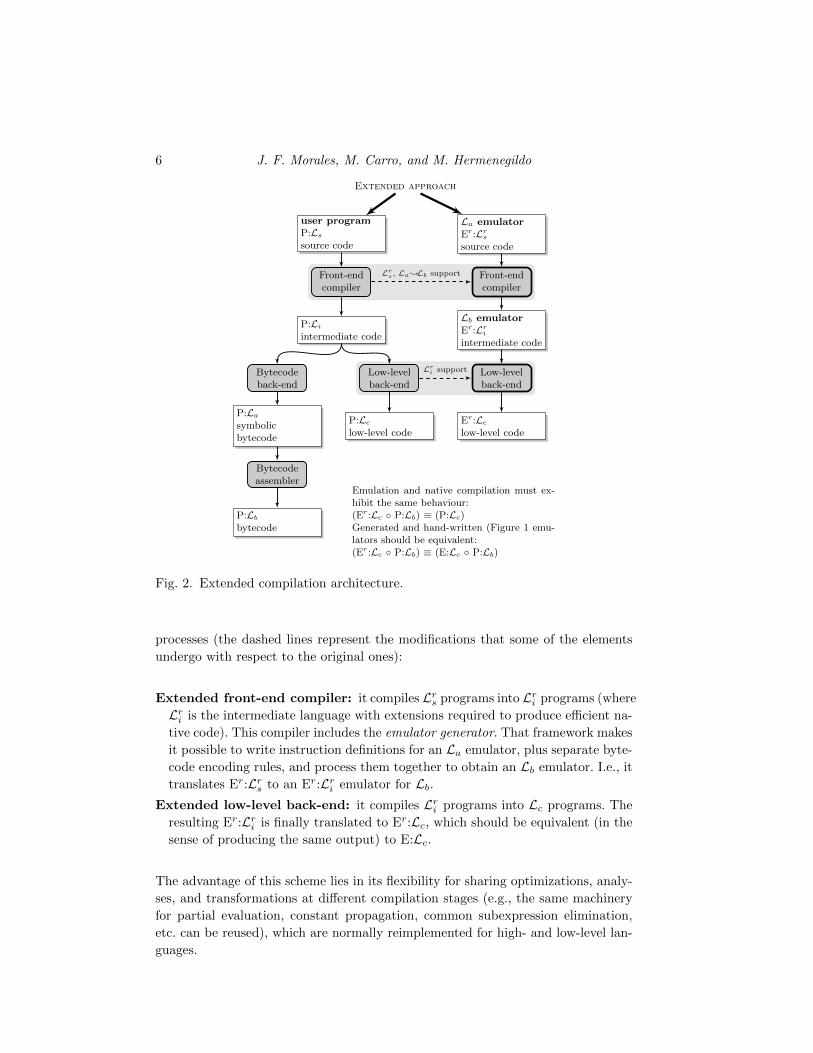
3.4.4 Compilation of Predicates
The rules in the previous sections defined how goals are compiled. In this section we
will use those rules to compile predicates as C functions. Figure 9 provides rules that
distinguish between deterministic and semi-deterministic predicates. For a predicate
with name = f /n, the lookup(name) function returns its arguments and body. The
information from analysis of encoding types and reference modes (Section 3.3) is
used by argdecls and vardecls to obtain the list of argument and variable declarations
for the program. On the other hand, bb code is a predefined operation that flattens
the basic blocks in its second argument θ as a C block composed of labels and
statements. Finally, the emitdecl operation is responsible for inserting the function
declarations in the compilation output p. Those definitions are used in the (Pred-
D) and (Pred-S) rules. The former compiles deterministic predicates by binding
a single success to a return statement, and emits a C function returning no value.
The latter compiles semi-deterministic predicates by binding the continuations to
code that returns a true or false value depending on the success and failure status.
Note that this code matches exactly the scheme needed in Section 3.4.2 to perform
calls to imProlog predicates compiled as C functions.

Theory and Practice of Logic Programming 23
Source:
:– regtype flag/1 + low(int32).flag := off | on.:– pred p(+I ) :: flag.p(I ) :–
mflag(I, A),A = B,swmflag(B),A@ = on.
:– pred mflag/2 + unfold.mflag(I, X ) :–
X = initmut(flag, I ).:– pred swmflag(+I ) :: mut(flag).swmflag(X ) :–
swflag(X @, X 2),X ⇐ X 2.
:– pred swflag/2 + unfold.swflag(on, off).swflag(off, on).
Output:
1 bool p(int32 i) {2 int32 a;3 int32 *b;4 int32 t;5 b = &a;6 swmflag(b);7 t = a;8 if (t == 1) goto l1; else goto l2;9 l1: return TRUE;
10 l2: return FALSE;11 }12 void smwflag(int32 *x) {13 int32 t;14 int32 x2;15 t = *x;16 if (t == 1) goto l1; else goto l2;17 l1: x2 = 0;18 goto l3;19 l2: x2 = 1;20 l3: *x = x2;21 return;22 }
Fig. 10. imProlog compilation example
3.4.5 A Compilation Example
In order to clarify how the previous rules generate code, we include here a code
snippet (Figure 10) with several types of variables accessed both from the scope of
their first appearance, and from outside that frame. We show also how this code is
compiled into two C functions. Note that redundant jumps and labels have been
simplified. It is composed of an encoding type definition flag/1, two predicates that
are compiled to C functions (p/1 semi-deterministic, swmflag/1 deterministic), and
two predicates with annotations to unfold the code during preprocessing (mflag/2
and swflag/2). Note that by unfolding the mflag/2 predicate, a piece of illegal code
(passing a reference to a local mutable) becomes legal. Indeed, this kind of predicate
unfolding has proved to be a good, manageable replacement for the macros which
usually appear in emulators written in lower-level languages and which are often a
source of mistakes.
3.4.6 Related compilation schemes
Another compilation scheme which produces similar code is described in (Hender-
son and Somogyi 2002). There are, however, significant differences, of which we will
mention just a few. One of them is the source language and the constraints imposed
on it. In our case we aim at writing a WAM emulator in imProlog from which C
code is generated with the constraint that it has to be identical (or, at least, very
close) to a hand-written and hand-optimized emulator, including the implementa-
tion of the internal data structures. This has forced us to pay special attention to
the compilation and placement of data, use mutable variables, and ignore for now

24 J. F. Morales, M. Carro, and M. Hermenegildo
non-deterministic control. Also, in this work we use an intermediate representation
based on basic blocks, which makes it easier to interface with internal back-ends for
compilers other than GCC, such as LLVM (Lattner and Adve 2004) (which enables
JIT compilation from the same representation).
4 Extensions for Emulator Generation in imProlog
The dialect and compilation process that has been described so far is general enough
to express the instructions in a typical WAM emulator, given some basic built-ins
about operations on data types, memory stacks, and O.S. interface. However, com-
bining those pieces of code together to build an efficient emulator requires a compact
encoding of the bytecode language, and a bytecode fetching and dispatching loop
that usually needs a tight control on low-level data and operations that we have not
included in the imProlog language. In (Morales et al. 2005) we showed that it is
possible to automate the generation of the emulator from generic instruction defini-
tions and annotations stating how the bytecode is encoded and decoded. Moreover,
this process was found to be highly mechanizable, while making instruction code
easier to manage and other optimizations (such as instruction merging) easier to
perform. In this section we show how this approach is integrated in the compilation
process, by including the emulator generation as part of it.
4.1 Defining WAM instructions in imProlog
The definition of every WAM instruction in imProlog looks just like a regular predi-
cate, and the types, modes, etc. of each of their arguments have to be declared using
(Ciao) assertions. As an example, Figure 11 shows imProlog code corresponding to
the definition of an instruction which tries to unify a term and a constant. The
pred declaration states that the first argument is a mutable variable and that the
second is a tagged word containing a constant. It includes a sample implementation
of the WAM dereference operation, which follows a reference chain and stops when
the value pointed to is the same as the pointing term, or when the chain cannot
be followed any more. Note the use of the native type tagged/2 and the operations
tagof/2 and tagval/2 which access the tag and the associated value of a tagged
word, respectively. Also note that the tagval/2 of a tagged word with ref results
in a mutable variable, as can be recognized in the code. Other native operations
include trail cond/1, trail push/1, and operations to manage the emulator stacks.
Note the special predicates next ins and fail ins. They execute the next instruction
or the failure instruction, respectively. The purpose of the next instruction is to
continue the emulation of the next bytecode instruction (which can be considered
as a recursive call to the emulator itself, but which will be defined as a built-in).
The failure instruction must take care of unwinding the stacks at the WAM level
and selecting the next bytecode instruction to execute (to implement the failure
in the emulator). As a usual instruction, it can be defined by calling built-ins or
other imProlog code, and it should finally include a call to next ins to continue the

Theory and Practice of Logic Programming 25
:– pred u cons(+, +) :: mut(tagged) * constagged.u cons(A, Cons) :–
deref(A@, T d),( tagof(T d, ref) → bind cons(T d, Cons), next ins; T d = Cons → next ins; fail ins).
:– pred deref/2.deref(T, T d) :–
( tagof(T, ref) →T 1 = ∼tagval(T )@,(T = T 1 → T d = T 1 ; deref(T 1, T d))
; T d = T).
:– pred bind/2.bind cons(Var, Cons) :–
(trail cond(Var) → trail push(Var) ; true),∼tagval(Var) ⇐ Cons.
Fig. 11. Unification with a constant and auxiliary definitions.
emulation. Since this instruction is often invoked from other instructions, a special
treatment is given to share its code, which will be described later.
The compilation process is able to unfold (if so desired) the definition of the
predicates called by u cons/2 and to propagate information inside the instruction,
in order to optimize the resulting piece of the emulator. After the set of trans-
formations that instruction definitions are subject to, and other optimizations on
the output (such as transformation of some recursions into loops) the generated C
code is of high quality (see, for example, Figure 14, for the code corresponding to
a specialization of this instruction).
Our approach has been to define a reduced number of instructions (50 is a ball-
park figure) and let the merging and specialization process (see Section 5) generate
all instructions needed to have a competitive emulator. Note that efficient emula-
tors tend to have a large number of instructions (hundreds, or even thousands, in
the case of Quintus Prolog) and many of them are variations (obtained through
specialization, merging, etc., normally done manually) on “common blocks.” These
common blocks are the simple instructions we aim at representing explicitly in
imProlog.
In the experiments we performed (Section 5.3) the emulator with a largest num-
ber of instructions had 199 different opcodes (not counting those which result from
padding some other instruction with zeroes to ensure a correct alignment in mem-
ory). A simple instruction set is easier to maintain and its consistency is easier to
ensure. Complex instructions are generated automatically in a (by construction)
sound way from this initial “seed.”

26 J. F. Morales, M. Carro, and M. Hermenegildo
mgen
La emulatorEr:Lr
s
source codeBytecodedefinitions
Instruction def-initions in Lr
s
Machine M
Menc
Mdec
MargI
Mins′
MdefI
Menc
Mins′ La to Lb
back-end
...
Ls to Lb compiler
emucompMdec
MargI
Mins′
MdefI
Lb emulatorEr:Lc
low-level code
Fig. 12. From imProlog definitions to Lb emulator in Lc.
4.2 An Emulator Specification in imProlog
Although imProlog could be powerful enough to describe the emulation loop, as
mentioned before we leverage on previous work (Morales et al. 2005) in which Lc
emulators were automatically built from definitions of instructions written in La and
their corresponding code written in Lc. Bytecode representation, compiler back-end,
and an emulator (including the emulator loop) able to understand Lb code can be
automatically generated from those components. In our current setting, definitions
for La instructions are written in Lrs (recall Figure 2) and these definitions can be
automatically translated into Lc by the imProlog compiler. We are thus spared of
making this compiler more complex than needed. More details on this process will
be given in the following section.
4.3 Assembling the Emulator
We will describe now the process that takes an imProlog representation of an ab-
stract machine and obtains a full-fledged implementation of this machine. The over-
all process is sketched in Figure 12, and can be divided into two stages, which we
have termed mgen and emucomp. The emulator definition, E , is a set of predicates
and assertions written in imProlog, and mgen is basically a normalization process
where the source E is processed to obtain a machine definition M. This definition
contains components describing the instruction semantics written in imProlog and
a set of hints about the bytecode representation (e.g., numbers for the bytecode
instructions). M is then processed by an emulator compiler emucomp which gen-
erates a bytecode emulator for the language Lb, written in the language Lc. The
machinery to encode La programs into the bytecode representation Lb is also given
by definitions in M.
Using the terminology in (Morales et al. 2005), we denote the components of Mas follows:
M = (Menc, Mdec, MargI , MdefI , Mins′)

Theory and Practice of Logic Programming 27
First, the relation between La and Lb is given by means of several components:12
Menc declares how the bytecode encodes La instructions and data: e.g., X(0) is
encoded as the number 0 for an instruction which needs access to some X register.
Mdec declares how the bytecode should be decoded to give back the initial instruc-
tion format in La: e.g., for an instruction which uses as argument an X register,
a 0 means X(0).
The remaining of the components of M capture the meaning of the (rather low
level) constituents of La, providing a description of each instruction. Those com-
ponents do not make bytecode representation issues explicit, as they have already
been specified in Menc and Mdec. In the present work definitions for La instruc-
tions are given in Lrs, instead of in Lc as was done in the formalization presented
in (Morales et al. 2005). The reason for this change is that in (Morales et al. 2005)
the final implementation language (Lc, in which emulators were generated) was
also the language in which each basic instruction was assumed to be written. How-
ever, in our case, instructions are obviously written in Lrs (i.e., imProlog, which is
more amenable to automatic program transformations) and it makes more sense
to use it directly in the definition of M. Using Lrs requires, however, extending
and/or modifying the remaining parts of M with respect to the original definition
as follows:
MargI which assigns a pair (T,mem) to every expression in La, where T is the
type of the expression and mem is the translation of the expression into Lc. For
example, the type of X(0) is mut(tagged) and its memory location is &(x[0]),
assuming X registers end up in an array.13
MdefI which contains the definition of each instruction in Lrs.
Mins′ which describes the instruction set with opcode numbers and the format
of each instruction, i.e., the type in La for each instruction argument: e.g., X
registers, Y registers, integers, atoms, functors.
The rest of the components and Mins′ are used by the emulator compiler to
generate an Lb emulator written in Lc. A summarized definition of the emulator
compiler and how it uses the different pieces in M can be found in Figure 13.
The (Emu) rule defines a function that contains the emulator loop. It is similar
to the (Pred-D) rule already presented, but takes parts of the source code from
M. It generates a list of basic block identifiers for each instruction, and a basic
block identifier for the emulator loop entry. The (Swr) rule is used to insert a
switch statement that implements the opcode fetching, and jumps to the code of
each instruction. The (Ins) rule is used to generate the code for each instruction.
To implement the built-ins next ins and fail ins, two special continuations ni and fi
are stored in the continuation mapping. The continuation to the failure instruction
is bound to the δf basic block identifier (assuming that the opf opcode is that
12 The complete description includes all elements for a WAM: X and Y registers, atoms, numbers,functors, etc.
13 This definition has been expanded with respect to its originalMarg definition in order to includethe imProlog type in addition to the memory location.

28 J. F. Morales, M. Carro, and M. Hermenegildo
(Emu)
Mops = [op1, ..., opn]θ0 = bb empty〈θ0〉 bb newn(n + 1) ⇒ [δ, δ1, ..., δn] 〈θ1〉〈θ1〉 emit switch(get_opcode(), Mops, [δ1, ..., δn], δ) ⇒ 〈θ2〉〈θ2〉 ∀i=1..n inscomp(opi, δ, δi, [fi7→δf ]) 〈θ〉code = bb code(δ, θ)〈p0〉 emitdecl(void emu() { code }) ⇒ 〈p〉
〈p0〉 emucomp ⇒ 〈p〉
(Swr)〈θ0〉 emit(switch (x) {case v1: goto δ1; ...; case vn: goto δn; }, δ) ⇒ 〈θ〉
〈θ0〉 emit switch(x, [v1, ..., vn], [δ1, ..., δn], δ) ⇒ 〈θ〉
(Ins)
(body, nextp) = insdef(opcode)〈θ2〉 gcomp(body, η[ni7→(δ0, nextp)], δ) ⇒ 〈θ〉〈θ0〉 inscomp(opcode, δ0, δ, η) ⇒ 〈θ〉
(NextIns)
(δs, nextp) = η(ni)〈θ0〉 emit(nextp, δ) ⇒ 〈θ1〉〈θ1〉 emit(goto δs, δ) ⇒ 〈θ〉
〈θ0〉 gcomp(next ins, η, δ) ⇒ 〈θ〉 (FailIns)
δs = η(fi)〈θ0〉 emit(goto δs, δ) ⇒ 〈θ〉〈θ0〉 gcomp(fail ins, η, δ) ⇒ 〈θ〉
Fig. 13. Emulator compiler.
of the failure instruction). The (FailIns) rule includes a special case in gcomp
that implements this call. The continuation to the next instruction is a pair of the
basic block that begins the emulator switch, and a piece of C code that moves the
bytecode pointer to the next instruction (that is particular to each instruction, and
is returned by insdef alongside with its code). The (NextIns) rule emits code that
executes that code and jumps to opcode fetching.
The abstract machine component Mins′ is used to obtain the name and data
format of the instruction identified by a given opcode. From the format andMargI
definition, a type, an encoding type, and a custom r-value for each instruction
argument are filled. In this way, the compilation process can transparently work
with variables whose value is defined from the operand information in a bytecode
stream (e.g., an integer, a machine register, etc.).
Relation with Other Compilation Schemes. The scheme of the generated emulator
code is somewhat similar to what the Janus compilation scheme (Gudeman et al.
1992) produces for general programs. In Janus, addresses for continuations are either
known statically (e.g., for calls, and therefore a direct, static jump to a label can
be performed) or are popped from the stack when returning. Since labels cannot
be directly assigned to variables in standard C, an implementation workaround is
made by assigning a number to each possible return address (and it is this number
which is pushed onto / popped from the stack) and using a switch to relate these
numbers with the code executing them. In our case we have a similar switch, but
it relates each opcode with its corresponding instruction code, and it is executed
every time a new instruction is dispatched.
We want to note that we deliberately stay within standard C in this presentation:
taking advantage of C extensions, such as storing labels in variables, which are
provided by gcc and used, for example, in (Henderson et al. 1995; Codognet and
Diaz 1995), is out of the scope of this paper. These optimizations are not difficult

Theory and Practice of Logic Programming 29
1 loop:2 switch(Op(short,P,0)) {3 ...4 case 97: goto ux_cons;5 ...6 }7 ...8 ux_cons:9 tagged t;
10 t = X(Op(short,P,2));11 deref(&t);12 if (tagged_tag(t) != REF)13 goto ux_cons__0;14 bind_cons(t, Op(tagged,P,4));15 goto ux_cons__1;16 ux_cons__0:17 if (t != Op(tagged,P,4))18 goto fail_ins;19 ux_cons__1:20 P = Skip(P,8);21 goto loop;22 ...
1 void deref(tagged_t *a0) {2 tagged_t t0;3 deref:4 if (tagged_tag(*a0) == REF)5 goto deref__0;6 else goto deref__1;7 deref__0:8 t0 = *(tagged_val(*a0));9 if ((*a0) != t0)
10 goto deref__2;11 else goto deref__1;12 deref__2:13 *a0 = t0;14 goto deref;15 deref__1:16 return;17 }
Fig. 14. Code generated for a simple instruction.
to add as code generation options, and therefore they should not be part of a basic
scheme. Besides, that would make it difficult to use compilers other than gcc.
Example 4.1
As an example, from the instruction in Figure 11, which unifies a term living in
some variable with a constant, we can derive a specialized version in which the term
is assumed to live in an X register. The declaration:
:– ins alias(ux cons, u cons(xreg mutable, constagged)).
assigns the (symbolic) name ux cons to the new instruction, and specifies that the
first argument lives in an X register. The declaration:
:– ins entry(ux cons).
indicates that the emulator has an entry for that instruction.14 Figure 14 shows the
code generated for the instruction (right) and a fragment of the emulator generated
by the emulator compiler in Figure 13.
14 We optionally allow a pre-assignment of an opcode number to each instruction entry. Differentassignments of instruction numbers to opcodes can impact the final performance, as they dictatehow the code is laid out in the emulator switch which affects, for example, the behavior of thecache.

30 J. F. Morales, M. Carro, and M. Hermenegildo
E M L emu prgB Bencode
prg A
ptransetrans
Mmgen emucomp
E’ M’ L emu prgB’ B’ encodeprg A’
M’
mgenemucomp
emulatorgeneration
programexecution
programcompilation
initial state final state
prg P
front-endcompiler
Fig. 15. Application of an instruction set transformation (ptrans, etrans).
5 Automatic Generation of Abstract Machine Variations
Using the techniques described in the previous section we now address how abstract
machine variations can be generated automatically. Substantial work has been de-
voted to abstract machine generation strategies such as, e.g., (Demoen and Nguyen
2000; Nassen et al. 2001; Zhou 2007), which explore different design variations with
the objective of putting together highly optimized emulators. However, as shown
previously, by making the semantics of the abstract machine instructions explicit
in a language like imProlog, which is easily amenable to automatic processing, such
variations can be formulated in a straightforward way mostly as automatic trans-
formations. Adding new transformation rules and testing them together with the
existing ones becomes then a relatively easy task.
We will briefly describe some of these transformations, which will be experimen-
tally evaluated in Section 5.3. Each transformation is identified by a two-letter
code. We make a distinction between transformations which change the instruc-
tion set (by creating new instructions) and those which only affect the way code is
generated.
5.1 Instruction Set Transformations
Let us define an instruction set transformation as a pair (ptrans,etrans), so that
ptrans transforms programs from two symbolic bytecode languages La and (a pos-
sibly different) La’ 15 and etrans transforms the abstract machine definition within
Lrs. Figure 15 depicts the relation between emulator generation, program compi-
lation, program execution, and instruction set transformations. The full emulator
generation includes etrans as preprocessing before mgen is performed. The resulting
emulator is able to interpret transformed programs after ptrans is applied (before
15 Those languages can be different, for example, if the transformation adds or removes someinstructions
Theory and Practice of Logic Programming 31
bytecode encoding), that is, the new compiler is obtained by including ptrans as a
new compilation phase.
Note that both ptrans and etrans are working at the symbolic bytecode level.
It is easier to work with a symbolic La program than with the stream of bytes
that represents Lb code, and it is easier to transform instructions written in Lrs and
specified at the La level, than those already written in Lc code (where references to
Lb code and implementation details obscure the actual semantics). Reasoning about
the correctness of the global transformation that affects the La program and the
instruction code is also easier in the Lrs specification of the emulator instructions
than in a low-level Lc emulator (assuming the correctness of the emulator generation
process).
In the following sections we will review the instruction set transformations cur-
rently available. Although more transformations can of course be applied, the cur-
rent set is designed with the aim of generating, from simple imProlog definitions,
an emulator which is as efficient as a hand-crafted, carefully tuned one.
5.1.1 Instruction Merging [im]
Instruction Merging generates larger instructions from sequences of smaller ones,
and is aimed at saving fetch cycles at the expense of a larger instruction set and,
therefore, an increased switch size. This technique has been used extensively in high-
performance systems (e.g., Quintus Prolog, SICStus, Yap, etc.). The performance
of different combinations has been studied empirically (Nassen et al. 2001), but
in that work new instructions were generated by hand, although deciding which
instructions had to be created was done by means of profiling. In our framework
only a single declaration is needed to emit code for a new, merged instruction.
Merging is done automatically through code unfolding and based on the definitions
of the component instructions. This makes it possible, in principle, to define a set
of (experimentally) optimal merging rules. However, finding exactly this set of rules
is actually not straightforward.
Merging rules are specified separately from the instruction code itself, and these
rules state how basic instructions have to be combined. To start with, we will need
to show how instructions are defined based on their abstract versions. For example,
definition:
move(A, B) :– B ⇐ A@ .
moves data between two locations, i.e., the contents of the a mutable into the b
mutable. In order to specify precisely the source and destination of the data, it is
necessary to specify the instruction format, with a declaration such as:
:– ins alias(movexy, move(xreg mutable, yreg mutable)).
which defines a virtual instruction named movexy, that corresponds to the instan-
tiation of the code for move/2 for the case in which the first argument corresponds

32 J. F. Morales, M. Carro, and M. Hermenegildo
to an X register and the second one corresponds to a Y register. Both registers are
seen from imProlog as mutable variables of type mut(tagged). Then, and based on
this more concrete instruction, the declaration:
:– ins entry(movexy + movexy).
forces the compiler to actually use during compilation an instruction composed of
two virtual ones and to emit bytecode containing it (thanks to the ptrans transfor-
mation in Figure 15, which processes the program instruction sequence to replace
occurrences of the collapsed pattern by the new instruction). Emulator code will
be generated implementing an instruction which merges two movexy instructions
(thanks to the etrans transformation). The corresponding code is equivalent to:
:– ins entry(movexy movexy).
:– pred movexy movexy(xreg mutable, yreg mutable,
xreg mutable, yreg mutable).
movexy movexy(A, B, C, D) :– B ⇐ A@, D ⇐ C @ .
This can later be subject to other transformations and used to generate emulator
code as any other imProlog instruction.
5.1.2 Single-Instruction Encoding of Sequences of the Same Instruction [ie]
In some cases a series of similar instructions (e.g., unify with void) with different
arguments can be collapsed into a single instruction with a series of operands which
correspond to the arguments of each of the initial instructions. For example, a
bytecode sequence such as:
unify with void(x(1)), unify with void(x(2)), unify with void(x(5))
can be compiled into:
unify with void n([x(1), x(2), x(5)])
which would perform exactly as in the initial instruction series, but taking less space
and needing fewer fetch cycles. Such an instruction can be created, emitted, and
the corresponding emulator code generated automatically based on the definition
of unify with void.
In order to express this composite instruction within imProlog using a single pred-
icate, unify with void n needs to receive a fixed number of arguments. A different
predicate for each of the possible lengths of the array would have to be generated
otherwise. A single argument actually suffices; hence the square brackets, which are
meant to denote an array.
The imProlog code which corresponds to the newly generated instruction is, con-
ceptually, as follows:
Theory and Practice of Logic Programming 33
unify with void n(Array) :–
array len(Array, L),
unify with void n 2(0, L, Array).
unify with void n 2(I, L, Array) :–
( I = L → true
; elem(I, Array, E ),
unify with void(E ),
I 1 is I + 1,
unify with void n 2(I 1, L, Array)
).
It should be clear here why a fixed number of arguments is needed: a series of
unify with void n/1, unify with void n/2, etc. would have to be generated otherwise.
Note that the loop code ultimately calls unify with void/1, the Lrs reflection of the
initial instruction.
In this particular case the compiler to Lc performs some optimizations not cap-
tured in the previous code. For example, instead of traversing explicitly the array
with an index, this array is expanded and inlined in the bytecode and the program
counter is used to retrieve the indexes of the registers by incrementing it after every
access. As the length of the array is known when the bytecode is generated, it is
actually explicitly encoded in the final bytecode. Therefore, all of the newly intro-
duced operations (array len/2, elem/3, etc.) need constant time and are compiled
efficiently.
5.1.3 Instructions for Special Built-Ins [ib]
As mentioned before, calling external library code or internal predicates (classically
termed “built-ins”) requires following a protocol, to pass the arguments, to check
for failure, etc. Although the protocol can be the same as for normal predicates
(e.g., passing arguments as X registers), some built-ins require a special (more effi-
cient) protocol (e.g., passing arguments as Lc arguments, avoiding movements in X
registers). Calling those special built-ins is, by default, taken care of by a generic
family of instructions, one per arity. This is represented as the instructions:
:– ins alias(bltin1d, bltin1(bltindet(tagged), xreg)).
bltin1(BltName, A) :– BltName(A@).
:– ins alias(bltin2d, bltin2(bltindet(tagged, tagged), xreg, xreg)).
bltin2(BltName, A, B) :– BltName(A@, B@).
where each bltinI/i + 1 acts as a bridge to call the external code expecting i param-
eters. The BltName argument represents a predicate abstraction that will contain
a reference to the actual code of the built-in during the execution. The type of the
BltName argument reflects the accepted calling pattern of the predicate abstrac-
tion. When compiling those instructions to Lc code, that predicate abstraction is

34 J. F. Morales, M. Carro, and M. Hermenegildo
efficiently translated as an unboxed pointer to an Lc procedure.16 With the def-
inition shown above, the imProlog compiler can generate, for different arities, an
instruction which calls the built-in passed as first argument.
However, by specifying at compile time a predefined set of built-ins or predicates
written in Lc (that is, a static value for BltName instead of a dynamic value), the
corresponding instructions can be statically specialized and an instruction set which
performs direct calls to the corresponding built-ins can be generated. This saves an
operand, generating slightly smaller code, and replaces an indirection by a direct
call, which saves memory accesses and helps the processor pipeline, producing faster
code.
5.2 Transformations of Instruction Code
Some transformations do not create new instructions; they perform instead a num-
ber of optimizations on already existing instructions by manipulating the code or
by applying selectively alternative translation schemes.
5.2.1 Unfolding Rules [ur]
Simple predicates can be unfolded before compilation. In the case of instruction
merging, unfolding is used to merge two (or more) instructions into a single piece of
code, in order to avoid fetch cycles (Section 5.1.1). However, uncontrolled unfolding
is not always an advantage, because an increased emulator size can affect negatively
the cache behavior. Therefore the ur option turns on or off a predefined set of rules
to control which instruction mergings are actually performed. Unfolding rules follow
the scheme:
:– ins entry(Ins1 + Ins2 + ... + Insn, WhatToUnfold).
where Ins1 to Insn are the basic instructions to be merged, and WhatToUnfold is a
rule specifying exactly which instruction(s) has to be unfolded when ur is activated.
As a concrete example, the unfolding rule:
:– ins entry(alloc + movexy + movexy, 1).
means that in the instruction to be generated by combining one alloc and two
movexy, the code for alloc is inlined (the value of the last argument 1 refers to
the first instruction in the sequence), and the (shared) code for movexy + movexy
is invoked afterwards. A companion instruction merging rule for movexy + movexy
exists:
16 In the bytecode, the argument that corresponds to the predicate abstraction is stored as anumber that uniquely identifies the built-in. When the bytecode is actually loaded, this numberis used to look up the actual address of the built-in in a table maintained at runtime. This isneeded since, in general, there is no way to know which address will be assigned to the entrypoint of a given built-in in different program executions.

Theory and Practice of Logic Programming 35
:– ins entry(movexy + movexy, all).
which states that the code for both movexy has to be unfolded in a combined
instruction. The instruction alloc + movexy + movexy would generate code for alloc
plus a call to movexy + movexy. The compiler eventually replaces this call by an
explicit jump to the location of movexy + movexy in the emulator. The program
counter is updated accordingly to access the arguments correctly.
5.2.2 Alternative Tag Switching Schemes [ts]
Tags are used to determine dynamically the type of basic data (atoms, structures,
numbers, variables, etc.) contained in a (tagged) memory word. Many instructions
and built-ins (like unification) take different actions depending on the type (or tag)
of the input arguments. This is called tag switching, and it is a heavily-used opera-
tion which is therefore worth optimizing as much as possible. The tag is identified
(and the corresponding action taken) using tag switching such as:
(tagtest1 → tagcode1 ; ... ; tagtestn → tagcoden)
where every tagtest i has the form tagof(v, tag i) (i.e., code that performs a different
action depending on the tag value of a tagged v). The ts option chooses between
either a switch control structure (when enabled) or a set of predefined test patterns
based on tag encodings and assertions on the possible tags (when disabled).
Both possibilities are studied in more detail in (Morales et al. 2008). Since the
numbers that encode the tags are usually small, it is easy for a modern C compiler
(e.g., gcc) to generate an indirection table and jump to the right code using it
(that is, it does not require a linear search). It is difficult, however, to make the C
compiler aware that checks to ensure that the tag number will actually be one of
the cases in the switch are, by construction, unnecessary (i.e., there is no need for
a default case). This information could be propagated to the compiler with a type
system which not all low-level languages have. The alternative compilation scheme
(rule (Tif)) makes explicit use of tag-checking primitives, where the sequence of
ctest i and the code of each branch depends on the particular case.
The latter approach is somewhat longer (and more complex as the number of
allowed tags grows) than the former. However, in some cases there are several
advantages to the latter, besides the already mentioned avoidance of boundary
checks:
• Tags with higher runtime probability can be checked before, in order to select
the right branch as soon as possible.
• Since the evaluation order is completely defined, tests can be specialized to
determine as fast as possible which alternative holds. For example, if by ini-
tial assumption v can only be either a heap variable, a stack variable, or a
structure (having a different tag for each case), then the tests can check if it
is a heap variable or a stack variable and assume that it is a structure in the
last branch.

36 J. F. Morales, M. Carro, and M. Hermenegildo
Deciding on the best option has to be based on experimentation, the results of
which we summarize in Section 5.3.3 and in tables 4 and 5.
5.2.3 Connected Continuations [cc]
Some actions can be repeated unnecessarily because they appear at the end of an
operation and at the beginning of the next one. Often they have no effect the second
time they are called (because they are, e.g., tests which do not change the tested
data, or data movements). In the case of tests, for example, they are bound to fail
or succeed depending on what happened in the previous invocation.
As an example, in the fragment deref(T ), (tagof(T, ref)→ A ; B) the test tagof(R,
ref) is performed just before exiting deref/1 (see Figure 11). Code generation for
instructions which include similar patterns is able to insert a jump either to A
or B from the code generated for deref/1. This option enables or disables this
optimization for a series of preselected cases, by means of code annotations similar
to the ones already shown.
5.2.4 Read/Write Mode Specialization [rw]
WAM-based implementations use a flag to test whether heap structures are being
read (matched against) or written (created). According to the value of this flag,
which is set by code executed immediately before, several instructions adapt their
behavior with an internal, local if-then-else.
A common optimization is to partially evaluate the switch statement which imple-
ments the fetch-and-execute cycle inside the emulator loop. Two different switches
can be generated, with the same structure, but with heap-related instructions spe-
cialized to perform either reads or writes (Carlsson 1996). Enabling or disabling
the rw optimization makes it possible to generate instruction sets (and emulators)
where this transformation has been turned on or off.
This is conceptually performed by generating different versions of the code for
the instructions, depending on the value of a mutable variable mode, which can only
take the values read or write. Deciding whether to generate different code versions
or to generate if-then-elses to be checked at run-time is done based on a series of
heuristics which try to forecast the complexity and size of the resulting code.
5.3 Experimental Evaluation
We present in this section experimental data regarding the performance achieved
on a set of benchmarks by a collection of emulators, all of which were automatically
generated by selecting different combinations of the options presented in previous
sections. In particular, by using all compatible possibilities for the transformation
and generation options given in Section 5 we generated 96 different emulators (in-
stead of 27 = 128, as not all options are independent; for example, ie needs im to
be performed). This bears a close relationship with (Demoen and Nguyen 2000),
but here we are not changing the internal data structure representation (and of

Theory and Practice of Logic Programming 37
course our instructions are all initially coded in imProlog). It is also related to the
experiment reported in (Nassen et al. 2001), but the tests we perform are more
extensive and cover more variations on the kind of changes that the abstract ma-
chine is subject to. Also, (Nassen et al. 2001) starts off by being selective about the
instructions to merge, which may seem a good idea but, given the very intricate
dependencies among different optimizations, can also result in a loss of optimization
opportunities. In any case, this is certainly a point we want to address in the future
by using instruction-level profiling.
Although most of the benchmarks we used are relatively well known, a brief
description follows:
boyer Simplified Boyer-Moore theorem prover kernel.
crypt Cryptoarithmetic puzzle involving multiplication.
deriv Symbolic derivation of polynomials.
factorial Compute the factorial of a number.
fib Simply recursive computation of the nth Fibonacci number.
knights Chess knight tour, visiting only once every board cell.
nreverse Naive reversal of a list using append.
poly Raises symbolically the expression 1 + x + y + z to the nth power.
primes Sieve of Eratosthenes.
qsort Implementation of QuickSort.
queens11 N -Queens with N = 11.query Makes a natural language query to a knowledge database with infor-
mation about country names, population, and area.
tak Computation of the Takeuchi function.
Our starting point was a “bare” instruction set comprising the common basic
blocks of a relatively efficient abstract machine (the “optimized” abstract machine
of Ciao 1.13, in the ‘optim comp’ directory of the Ciao 1.13 repository).17 The
Ciao abstract machines have their remote roots in the emulator of SICStus Prolog
0.5/0.7 (1986-89), but have evolved over the years quite independently and been
the object of many optimizations and code rewrites resulting in performance im-
provements and much added functionality.18 The performance of this, our baseline
engine matches that of modern Prolog implementations. Table 2 helps evaluating
the speed of this baseline optimized Ciao emulator w.r.t. to the relatively unop-
timized Ciao 1.13 emulator compiled by default in the Ciao distribution, some
high-performance Prolog implementations (Yap 5.1.2 (Santos-Costa et al. 2011)
and hProlog 2.7 (Demoen 2012)), and the popular SWI-Prolog system (version
5.6.55 (Wielemaker 2010)).
Figures 16 (in page 39) to 37 (in page 47) summarize graphically the results of
the experiments, as the data gathered —96 emulators × 13 benchmarks = 1248
performance figures— is too large to be comfortably presented in regular tables.
17 Changes in the optimized version include tweaks to clause jumping, arithmetic operations andbuilt-ins and some code clean-ups that reduce the size of the emulator loop.
18 This includes modules, attributed variables, support for higher order, multiprocessing, paral-lelism, tabling, modern memory management, etc., etc.

38 J. F. Morales, M. Carro, and M. Hermenegildo
Benchmark Yap hProlog SWI Ciao-std Ciao-opt5.1.2 2.7 5.6.55 1.13 (baseline)
boyer 1392 1532 11169 2560 1604crypt 3208 2108 36159 6308 3460deriv 3924 3824 12610 6676 3860exp 1308 1740 2599 1400 1624factorial 4928 2368 16979 3404 2736fft 1020 1652 14351 2236 1548fib 2424 1180 8159 1416 1332knights 2116 1968 11980 3432 2352nreverse 1820 908 18950 3900 2216poly 1328 1104 6850 1896 1160primes 4060 2004 28050 3936 2520qsort 1604 1528 8810 2600 1704queens11 1408 1308 24669 3200 1676query 632 676 6180 1448 968tak 3068 1816 27500 5124 2964
Table 2. Speed comparison of baseline with other Prolog systems.
Each figure presents the speedup obtained by different emulators for a given
benchmark (or all benchmarks in the case of the summary tables). Such speedups
are relative to some“default”code generation options, which we have set to be those
which were active in the Ciao emulator we started with (our baseline), and which
therefore receive speedup 1.0. Every point in each graph corresponds to the relative
speed of a different emulator obtained with a different combination of the options
presented in Sections 5.1 and 5.2.
The options are related to the points in the graphs as follows: each option is
assigned a bit in a binary number, where ‘1’ means activating the option and ‘0’
means deactivating it. Every value in the y axis of the figures corresponds to a
combination of the three options in Section 5.1. Note that only 6 combinations (out
of the 23 = 8 possible ones) are plotted due to dependencies among options (for
example, “Instruction encoding” always implies “Instruction merging”). The options
in Section 5.2, which correspond to transformations in the way code is generated
and which need four bits, are encoded using 24 = 16 different dot shapes. Every
combination of emulator generation options is thus assigned a different 7-bit number
encoded as a dot shape and a y coordinate. The x coordinate represents the speedup
as presented before (i.e., relative to the hand-coded emulator currently in Ciao 1.13).
The level of agressiveness of the instruction set transformations used in the paper
was selected to automatically generate an emulator identical to the hand-crafted
one. We have experimentally confirmed that it is difficult to outperform this engine
without changing other parameters, such as the overall architecture.
Different selections for the bits assigned to the y coordinate and to the dot shapes
would of course yield different plot configurations. However, our selection seems
intuitively appropriate, as it uses two different encodings for two different families
of transformations, one which affects the bytecode language itself, and another one
which changes the way these bytecode operands are interpreted. Table 3 relates the
bits in these two groups, using the same order as in the plots.

Theory and Practice of Logic Programming 39
Instruction InstructionGeneration Transformations
Instruction Special Instruction Tag Connected Unfolding R/WEncoding Builtins Merging Switching Conts. Rules Mode
(ie) (ib) (im) (ts) (cc) (ur) (rw)
Table 3. Meaning of the bits in the plots.
000
010
001
011
101
111
0.5 0.6 0.7 0.8 0.9 1 1.1 1.2 1.3
byte
co
de
ge
ne
ration
op
tion
s
0000100001001100001010100110111000011001010111010011101101111111
Fig. 16. Geometric average of all benchmarks (with a dot per emulator) — Intel.
Every benchmark was run several times on each emulator to make timings stable.
The hosts used were an x86 machine with a Pentium 4 processor running Linux
and an iMac with a PowerPC 7450 running Mac OS X. Arithmetic and geometric19
averages of all benchmarks were calculated and are shown in Figures 16, 17, 32,
and 33. Their similarity seems to indicate that there are no “odd” behaviors off
the average. Additionally, we are including detailed plots for every benchmark and
all the engine generation variants, following the aforementioned codification, first
for the x86 architecture (Figures 19 to 31) and then for the PowerPC architecture
(Figures 34 to 46), in the same order in both cases. Plots for specially relevant cases
are shown first, followed by the rest of the figures sorted following an approximate
(subjective) “more sparse” to “less sparse” order.
5.3.1 General Analysis
The best speedup among all tried options, averaged across the exercised benchmarks
and with respect to the baseline Ciao 1.13 emulator, is 1.05× for the x86 processor
(Table 4, top section, under the column w.r.t. def.) and 1.01× for the PowerPC
(Table 5, top section, same column heading). While this is a modest average gain,
some benchmarks achieve much better speedups. An alternative interpretation of
this result is that by starting with a relatively simple instruction set (coded directly
in imProlog) and applying automatically and systematically a set of transformation
and code generation options which can be trusted to be correct, we have managed
19 The geometric average is known to be less influenced by extremely good or bad cases.

40 J. F. Morales, M. Carro, and M. Hermenegildo
000
010
001
011
101
111
0.5 0.6 0.7 0.8 0.9 1 1.1 1.2 1.3
byte
co
de g
en
era
tion
op
tion
s
0000100001001100001010100110111000011001010111010011101101111111
Fig. 17. Arithmetic average of all benchmarks (with a dot per emulator) — Intel.
to match (and even exceed) the time performance of an emulator which was hand-
coded by very proficient programmers, and in which decisions were thoroughly
tested along several years. Memory usage was unaltered. Note (in the same tables)
that the speedup obtained with respect to the basic instruction set (under the
column labeled w.r.t. base) is significantly higher.
Figure 16 depicts the geometric average of the executions of all benchmarks in an
Intel platform. It aims at giving an intuitive feedback of the overall performance of
the option sets, and indeed a well defined clustering around eight centers is clear.
Figure 17, which uses the arithmetic average, is very similar (but not identical —
it is very slightly biased towards higher speedups), and it shows eight well-defined
clusters as well.
From these pictures we can infer that bytecode transformation options can be
divided into two different sets: one which is barely affected by options of the gen-
eration of code for the emulator (corresponding to the upper four clusters), and
another set (the bottom four clusters) in which changes to the generation of the
emulator code does have an effect in the performance.
In general, the results obtained in the PowerPC show fewer variations than those
obtained in an x86 processor. We attribute this behavior to differences between
these two architectures, as they greatly affect the optimization opportunities and the
way the C compiler can generate code. For example, the larger number of general-
purpose registers available in a PowerPC seems to make the job of the C compiler
less dependent on local variations of the code (as the transformations shown in Sec-
tion 5.2 produce). Additionally, internal differences between both processors (e.g.,
how branch prediction is performed, whether there is register renaming, shadow
registers, etc.) can also contribute to the differences we observed.
As a side note, while Figures 16 and 17 portray an average behavior, there were
benchmarks whose performance depiction actually match this average behavior
very faithfully —e.g., the simply recursive Factorial (Figure 19), which is often
disregarded as an unrealistic benchmark but which, for this particular experiment,
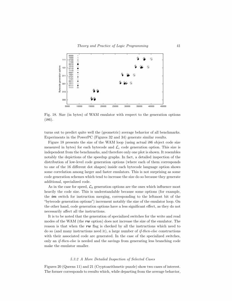
Theory and Practice of Logic Programming 41
000
010
001
011
101
111
5000 10000 15000 20000 25000 30000 35000 40000 45000
Byte
co
de g
en
era
tio
n o
ptio
ns
0000100001001100001010100110111000011001010111010011101101111111
Fig. 18. Size (in bytes) of WAM emulator with respect to the generation options
(i86).
turns out to predict quite well the (geometric) average behavior of all benchmarks.
Experiments in the PowerPC (Figures 32 and 34) generate similar results.
Figure 18 presents the size of the WAM loop (using actual i86 object code size
measured in bytes) for each bytecode and Lc code generation option. This size is
independent from the benchmarks, and therefore only one plot is shown. It resembles
notably the depictions of the speedup graphs. In fact, a detailed inspection of the
distribution of low-level code generation options (where each of them corresponds
to one of the 16 different dot shapes) inside each bytecode language option shows
some correlation among larger and faster emulators. This is not surprising as some
code generation schemes which tend to increase the size do so because they generate
additional, specialized code.
As in the case for speed, Lb generation options are the ones which influence most
heavily the code size. This is understandable because some options (for example,
the im switch for instruction merging, corresponding to the leftmost bit of the
“bytecode generation options”) increment notably the size of the emulator loop. On
the other hand, code generation options have a less significant effect, as they do not
necessarily affect all the instructions.
It is to be noted that the generation of specialized switches for the write and read
modes of the WAM (the rw option) does not increase the size of the emulator. The
reason is that when the rw flag is checked by all the instructions which need to
do so (and many instructions need it), a large number of if-then-else constructions
with their associated code are generated. In the case of the specialized switches,
only an if-then-else is needed and the savings from generating less branching code
make the emulator smaller.
5.3.2 A More Detailed Inspection of Selected Cases
Figures 20 (Queens 11) and 21 (Cryptoarithmetic puzzle) show two cases of interest.
The former corresponds to results which, while departing from the average behavior,

42 J. F. Morales, M. Carro, and M. Hermenegildo
000
010
001
011
101
111
0.5 0.6 0.7 0.8 0.9 1 1.1 1.2 1.3
byte
co
de g
en
era
tion
op
tion
s
0000100001001100001010100110111000011001010111010011101101111111
Fig. 19. Factorial involving large numbers — Intel.
000
010
001
011
101
111
0.5 0.6 0.7 0.8 0.9 1 1.1 1.2 1.3
byte
co
de
ge
ne
ratio
n o
ptio
ns
0000100001001100001010100110111000011001010111010011101101111111
Fig. 20. Queens (with 11 queens to place) — Intel.
000
010
001
011
101
111
0.5 0.6 0.7 0.8 0.9 1 1.1 1.2 1.3
byte
co
de
ge
ne
ratio
n o
ptio
ns
0000100001001100001010100110111000011001010111010011101101111111
Fig. 21. Cryptoarithmetic puzzle — Intel.

Theory and Practice of Logic Programming 43
000
010
001
011
101
111
0.5 0.6 0.7 0.8 0.9 1 1.1 1.2 1.3
byte
co
de g
en
era
tion
op
tion
s
0000100001001100001010100110111000011001010111010011101101111111
Fig. 22. Computation of the Takeuchi function — Intel.
000
010
001
011
101
111
0.5 0.6 0.7 0.8 0.9 1 1.1 1.2 1.3
byte
co
de
ge
ne
ratio
n o
ptio
ns
0000100001001100001010100110111000011001010111010011101101111111
Fig. 23. Symbolic derivation of polynomials — Intel.
000
010
001
011
101
111
0.5 0.6 0.7 0.8 0.9 1 1.1 1.2 1.3
byte
co
de
ge
ne
ratio
n o
ptio
ns
0000100001001100001010100110111000011001010111010011101101111111
Fig. 24. Naive reverse — Intel.

44 J. F. Morales, M. Carro, and M. Hermenegildo
000
010
001
011
101
111
0.5 0.6 0.7 0.8 0.9 1 1.1 1.2 1.3
byte
co
de g
en
era
tion
op
tion
s
0000100001001100001010100110111000011001010111010011101101111111
Fig. 25. Symbolic exponentiation of a polynomial — Intel.
000
010
001
011
101
111
0.5 0.6 0.7 0.8 0.9 1 1.1 1.2 1.3
byte
co
de
ge
ne
ratio
n o
ptio
ns
0000100001001100001010100110111000011001010111010011101101111111
Fig. 26. Version of Boyer-Moore theorem prover — Intel.
000
010
001
011
101
111
0.5 0.6 0.7 0.8 0.9 1 1.1 1.2 1.3
byte
co
de
ge
ne
ratio
n o
ptio
ns
0000100001001100001010100110111000011001010111010011101101111111
Fig. 27. QuickSort — Intel.

Theory and Practice of Logic Programming 45
000
010
001
011
101
111
0.5 0.6 0.7 0.8 0.9 1 1.1 1.2 1.3
byte
co
de g
en
era
tion
op
tion
s
0000100001001100001010100110111000011001010111010011101101111111
Fig. 28. Calculate primes using the sieve of Eratosthenes — Intel.
000
010
001
011
101
111
0.5 0.6 0.7 0.8 0.9 1 1.1 1.2 1.3
byte
co
de
ge
ne
ratio
n o
ptio
ns
0000100001001100001010100110111000011001010111010011101101111111
Fig. 29. Natural language query to a geographical database — Intel.
000
010
001
011
101
111
0.5 0.6 0.7 0.8 0.9 1 1.1 1.2 1.3
byte
co
de
ge
ne
ratio
n o
ptio
ns
0000100001001100001010100110111000011001010111010011101101111111
Fig. 30. Chess knights tour — Intel.
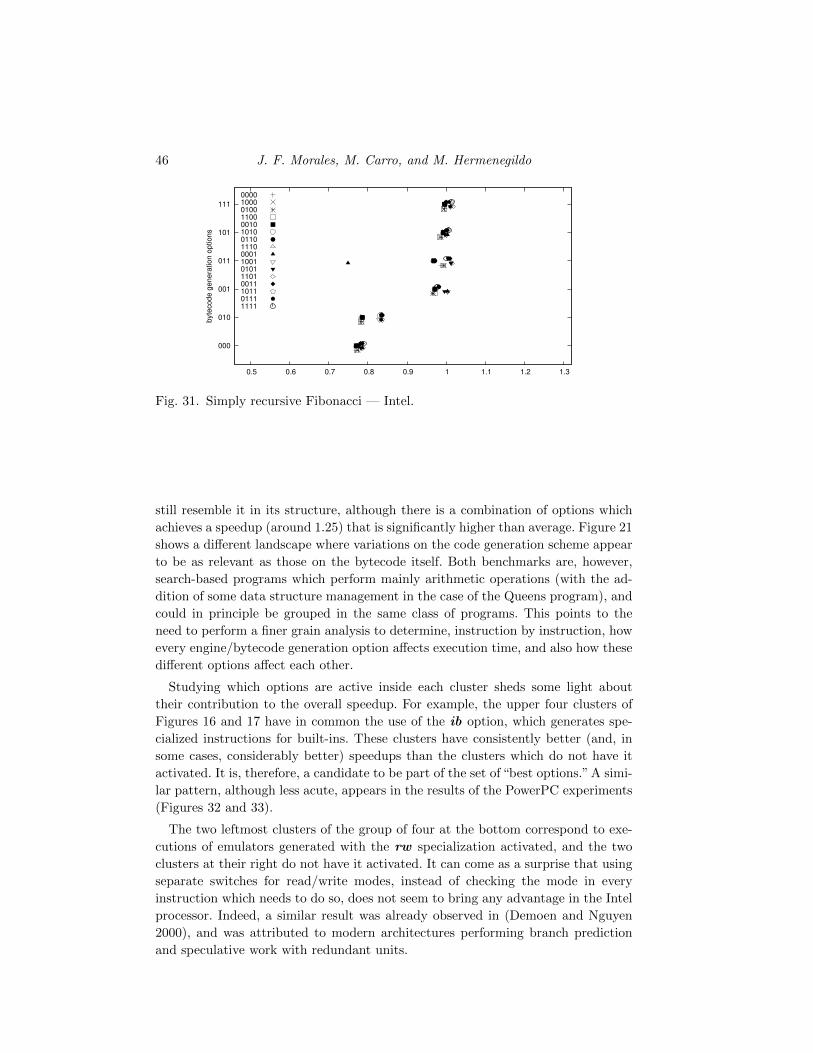
46 J. F. Morales, M. Carro, and M. Hermenegildo
000
010
001
011
101
111
0.5 0.6 0.7 0.8 0.9 1 1.1 1.2 1.3
byte
co
de g
en
era
tion
op
tion
s
0000100001001100001010100110111000011001010111010011101101111111
Fig. 31. Simply recursive Fibonacci — Intel.
still resemble it in its structure, although there is a combination of options which
achieves a speedup (around 1.25) that is significantly higher than average. Figure 21
shows a different landscape where variations on the code generation scheme appear
to be as relevant as those on the bytecode itself. Both benchmarks are, however,
search-based programs which perform mainly arithmetic operations (with the ad-
dition of some data structure management in the case of the Queens program), and
could in principle be grouped in the same class of programs. This points to the
need to perform a finer grain analysis to determine, instruction by instruction, how
every engine/bytecode generation option affects execution time, and also how these
different options affect each other.
Studying which options are active inside each cluster sheds some light about
their contribution to the overall speedup. For example, the upper four clusters of
Figures 16 and 17 have in common the use of the ib option, which generates spe-
cialized instructions for built-ins. These clusters have consistently better (and, in
some cases, considerably better) speedups than the clusters which do not have it
activated. It is, therefore, a candidate to be part of the set of “best options.” A simi-
lar pattern, although less acute, appears in the results of the PowerPC experiments
(Figures 32 and 33).
The two leftmost clusters of the group of four at the bottom correspond to exe-
cutions of emulators generated with the rw specialization activated, and the two
clusters at their right do not have it activated. It can come as a surprise that using
separate switches for read/write modes, instead of checking the mode in every
instruction which needs to do so, does not seem to bring any advantage in the Intel
processor. Indeed, a similar result was already observed in (Demoen and Nguyen
2000), and was attributed to modern architectures performing branch prediction
and speculative work with redundant units.

Theory and Practice of Logic Programming 47
000
010
001
011
101
111
0.5 0.6 0.7 0.8 0.9 1 1.1 1.2 1.3
byte
code g
enera
tion o
ptions
0000100001001100001010100110111000011001010111010011101101111111
Fig. 32. Geometric average of all bench-
marks (with a dot per emulator) — Pow-
erPC.
000
010
001
011
101
111
0.5 0.6 0.7 0.8 0.9 1 1.1 1.2 1.3
byte
code g
enera
tion o
ptions
0000100001001100001010100110111000011001010111010011101101111111
Fig. 33. Arithmetic average of all bench-
marks (with a dot per emulator) — Pow-
erPC.
000
010
001
011
101
111
0.5 0.6 0.7 0.8 0.9 1 1.1 1.2 1.3
byte
code g
enera
tion o
ptions
0000100001001100001010100110111000011001010111010011101101111111
Fig. 34. Factorial involving large num-
bers — PowerPC.
000
010
001
011
101
111
0.5 0.6 0.7 0.8 0.9 1 1.1 1.2 1.3
byte
code g
enera
tion o
ptions
0000100001001100001010100110111000011001010111010011101101111111
Fig. 35. Queens (with 11 queens to
place) — PowerPC.
000
010
001
011
101
111
0.5 0.6 0.7 0.8 0.9 1 1.1 1.2 1.3
byte
code g
enera
tion o
ptions
0000100001001100001010100110111000011001010111010011101101111111
Fig. 36. Cryptoarithmetic puzzle —
PowerPC.
000
010
001
011
101
111
0.5 0.6 0.7 0.8 0.9 1 1.1 1.2 1.3
byte
code g
enera
tion o
ptions
0000100001001100001010100110111000011001010111010011101101111111
Fig. 37. Computation of the Takeuchi
function — PowerPC.
000
010
001
011
101
111
0.5 0.6 0.7 0.8 0.9 1 1.1 1.2 1.3
byte
code g
enera
tion o
ptions
0000100001001100001010100110111000011001010111010011101101111111
Fig. 38. Symbolic derivation of polyno-
mials — PowerPC.
000
010
001
011
101
111
0.5 0.6 0.7 0.8 0.9 1 1.1 1.2 1.3
byte
code g
enera
tion o
ptions
0000100001001100001010100110111000011001010111010011101101111111
Fig. 39. Naive reverse — PowerPC.

48 J. F. Morales, M. Carro, and M. Hermenegildo
000
010
001
011
101
111
0.5 0.6 0.7 0.8 0.9 1 1.1 1.2 1.3
byte
code g
enera
tion o
ptions
0000100001001100001010100110111000011001010111010011101101111111
Fig. 40. Symbolic exponentiation of a
polynomial — PowerPC.
000
010
001
011
101
111
0.5 0.6 0.7 0.8 0.9 1 1.1 1.2 1.3
byte
code g
enera
tion o
ptions
0000100001001100001010100110111000011001010111010011101101111111
Fig. 41. Version of Boyer-Moore theorem
prover — PowerPC.
000
010
001
011
101
111
0.5 0.6 0.7 0.8 0.9 1 1.1 1.2 1.3
byte
code g
enera
tion o
ptions
0000100001001100001010100110111000011001010111010011101101111111
Fig. 42. QuickSort — PowerPC.
000
010
001
011
101
111
0.5 0.6 0.7 0.8 0.9 1 1.1 1.2 1.3
byte
code g
enera
tion o
ptions
0000100001001100001010100110111000011001010111010011101101111111
Fig. 43. Calculate primes using the sieve
of Eratosthenes — PowerPC.
000
010
001
011
101
111
0.5 0.6 0.7 0.8 0.9 1 1.1 1.2 1.3
byte
code g
enera
tion o
ptions
0000100001001100001010100110111000011001010111010011101101111111
Fig. 44. Natural language query to a ge-
ographical database — PowerPC.
000
010
001
011
101
111
0.5 0.6 0.7 0.8 0.9 1 1.1 1.2 1.3
byte
code g
enera
tion o
ptions
0000100001001100001010100110111000011001010111010011101101111111
Fig. 45. Chess knights tour — PowerPC.
000
010
001
011
101
111
0.5 0.6 0.7 0.8 0.9 1 1.1 1.2 1.3
byte
code g
enera
tion o
ptions
0000100001001100001010100110111000011001010111010011101101111111
Fig. 46. Simply recursive Fibonacci —
PowerPC.

Theory and Practice of Logic Programming 49
BenchmarkBest performance
ie ib im ts cc ur rw Speed-upbaseline x x x x x w.r.t. def. w.r.t. baseall (geom.) x x x x x 1.05 1.28boyer x x x x 1.18 1.52crypt x x x 1.22 1.07deriv x x x x 1.10 1.46factorial x x x 1.02 1.21fib x x x x x x 1.02 1.32knights x x x x 1.06 1.39nreverse x x x x 1.03 1.34poly x x x x x 1.02 1.52primes x x x x 1.10 1.26qsort x x x x 1.05 1.46queens11 x x x x x x x 1.26 1.46query x x x x x x 1.06 1.21tak x x x x 1.23 1.62
BenchmarkWorst performance
ie ib im ts cc ur rw Speed-upbaseline x x x x x w.r.t. def. w.r.t. baseall (geom.) x x 0.70 0.88boyer x 0.70 0.90crypt x x 0.86 0.75deriv x x 0.62 0.82factorial x x 0.76 0.99fib x x x 0.75 0.91knights x x x x 0.72 0.97nreverse x x x 0.57 0.95poly x x 0.56 0.74primes x x x 0.73 0.84qsort x x 0.54 0.84queens11 x x x 0.77 0.75query x x 0.71 0.89tak x x x x 0.69 0.92
Table 4. Options which gave best/worst performance (x86).
5.3.3 Best Generation Options and Overall Speedup
An important general question is which options should be used for the “stock” em-
ulator to be offered to general users. Our experimental results show that options
cannot be considered in isolation — i.e., the overall option set constructed by taking
separately the best value for every option does not yield a better set (defined as
the best options obtained by averaging speedups for every option set). As we have
seen, there is some interdependence among options. A more realistic answer is that
the average best set of options should come from selecting the rightmost point in
the plot corresponding to average speedups. We must however bear in mind that
averages always suffer the problem that a small set of good results may bias the

50 J. F. Morales, M. Carro, and M. Hermenegildo
BenchmarkBest performance
ie ib im ts cc ur rw Speed-upbaseline x x x x x w.r.t. def. w.r.t. baseall (geom.) x x x x x x 1.01 1.21boyer x x x x 1.02 1.25crypt x x x x 1.00 1.13deriv x x x x x 1.00 1.30factorial x x x x x 1.00 1.02fib x x x x 1.03 1.17knights x x x x 1.00 1.10nreverse x x x x 1.02 1.20poly x x x x x x 1.01 1.35primes x x x x x x 1.02 1.33qsort x x x x x x 1.01 1.17queens11 x x x x x 1.06 1.33query x x x x x x x 1.01 1.20tak x x x x x 1.01 1.22
BenchmarkWorst performance
ie ib im ts cc ur rw Speed-upbaseline x x x x x w.r.t. def. w.r.t. baseall (geom.) x 0.82 0.99boyer x x 0.81 0.99crypt x x x x 0.87 0.98deriv x x x 0.76 0.99factorial x x 0.85 0.97fib 0.94 0.99knights x x 0.82 1.00nreverse x x 0.74 0.98poly x 0.74 0.98primes x x 0.86 0.97qsort x 0.75 0.99queens11 x 0.88 0.99query x 0.82 0.99tak x x 0.78 0.99
Table 5. Options which gave best/worst performance (PowerPC).
average and, in this case, force the selection of an option set which performs worse
for a larger set of benchmarks
In order to look more closely at the effects of individual options (without re-
sorting to extensively listing them and the obtained performance), Tables 4 and 5
show which options produced the best and the worst results time-wise for each
benchmark. We include the geometric average as an specific case and the Ciao-1.10
baseline options as reference.
It has to be noted that the best/worst set of options is not the negation of the
worst/best options: there are plenty of cases where the same option was (de)activated
both for the best and for the worst executions. The observed situation for the Pow-
erPC architecture (Table 5) is more homogeneous: at least some better/worst be-
haviors really come from combinations which are complementary, and, in the cases

Theory and Practice of Logic Programming 51
where this is not so, the amount of non-complementary options goes typically from
1 to 3 — definitely less than in the x86 case.
Despite the complexity of the problem, some conclusions can be drawn: instruc-
tion merging (im) is a winner for the x86, probably followed by having a variable
number of operands (ie), and then by specialized calls to built-ins (ib). The first
and second options save fetch cycles, while the third one saves processing time in
general. It is to be noted that some options appear both in the best and worst cases:
this points to interdependencies among the different options.
The performance table for the PowerPC (Table 5) also reveals that instruction
merging, having a variable number of operands, and generating specialized instruc-
tions for built-ins, are options which bring performance advantages. However, and
unlike the x86 table, the read/write mode specialization is activated in all the lines
of the “best performance” table, and off in the “worst performance.” A similar case
is that of the tag switching schema, in the sense that the selection seems clear in
the PowerPC case.
The transformation rules we have applied in our case are of course not the only
possible ones, and we look forward to enlarging this set of transformations by, for
example, performing a more aggressive merging guided by profiling.20 Similar work,
with more emphasis on the production of languages for microprocessors is presented
in (Holmer 1993), where a set of benchmarks is used to guide the (constrained)
synthesis of such a set of instructions.
We want to note that although exceeding the speed of a hand-crafted emulator is
not the main concern in this work,21 the performance obtained by the implementa-
tion of the emulator in imProlog allows us to conclude that the imProlog approach
can match the performance of lower-level languages, while making it possible to
apply non-trivial program transformation techniques.
Additional experiments carried out in a very different context (that of embed-
ded systems and digital signal processing using Ciao Prolog (Carro et al. 2006),
which pertains to a realm traditionally considered disadvantageous for symbolic
languages) showed also very good performance —only 20% slower than a compa-
rable C program— and also very good speedups (up to 7-fold compared with a
bytecode-based implementation). Analysis and compilation techniques similar to
those applied in this paper were used, but put to work in a program using the full
Prolog language.
6 Conclusions
We have designed a language (imProlog, a variation of Prolog with some imperative
features) and its compiler, and we have used this language to describe the semantics
of the instructions of a bytecode interpreter (in particular, the Ciao engine). The
20 Merging is right now limited in depth to avoid a combinatorial explosion in the number ofinstructions.
21 In order to do that, a better approach would probably be to start off by finding performancebottlenecks in the current emulator and redesigning / recoding it. We want to note, however,that we think that our approach can greatly help in making this redesign and recoding easier.

52 J. F. Morales, M. Carro, and M. Hermenegildo
imProlog language, with the proposed constraints and extensions, is semantically
close enough to Prolog to share analysis, optimization and compilation techniques,
but at the same time it is designed to make translation into very efficient C code
possible. The low-level code for each instruction and the definition of the bytecode is
taken as input by a previously developed emulator generator to assemble full high-
quality emulators. Since the process of generating instruction code and bytecode
format is automatic, we were able to produce and test different versions thereof to
which several combinations of code generation options were applied.
Our main conclusion is that indeed the proposed approach can produce emulators
that are as efficient as the best state-of-the-art emulators hand-coded in C, while
starting from a much higher-level description. This high-level nature of the language
used allows avoiding some of the typical problems that hinder the development and
maintenance of highly-tuned emulators.
In our experience, in addition to greatly increased clarity and readability the port
allowed replacing many duplicated code structures, redundant hand-made special-
izations, and a large number of C macros (which notwithstanding do help in writing
less code, but they are not easily recognized in the source –leading often to pro-
grammer confusion–, they are prone to subtle scoping-related errors, and they are
typically not understood by automatic compilation tools), with more abstract pred-
icates, sometimes adorned with some annotations to guide the transformations.
The proposed approach makes it possible to perform non-trivial transformations
on both the emulator and the instruction level (e.g., unfolding and partial evaluation
of instruction definitions, instruction merging or specialization, etc.). The different
transformations and code generation options, result in different grades of optimiza-
tion / specialization and different bytecode languages from a single (higher-level)
abstract machine definition.
We have also studied how these combinations perform with a series of benchmarks
in order to find, e.g., what is the “best” average solution and how independent
coding rules affect the overall speed. We have in this way as one case the regular
emulator we started with (and which was decomposed to break complex instructions
into basic blocks). However, we also found out that it is possible to outperform it
slightly by using some code patterns and optimizations not explored in the initial
emulator, and, what is more important, starting from abstract machine definitions
in imProlog.
Performance evaluation of non-trivial variations in the emulator code showed
that some results are hard to predict and that there is no absolute winner for all
architectures and programs. On the other hand, it is increasingly difficult to reflect
all the variations in a single source using more traditional methods like m4 or cpp
macros. Automatic program manipulation at the emulator level represents a very
attractive approach, and although difficult, the problem becomes more tractable
when the abstraction level of the language to define the virtual machine is raised
and enriched with some problem-specific declarations.
As future work, it would be interesting to study the generation of efficient code for
full Prolog with imProlog features. A partial application of such compilation tech-

Theory and Practice of Logic Programming 53
niques was already put to work in the real-time digital sound processing application
written in Prolog mentioned before, with very successful results.
7 Acknowledgments
Acknowledgments: This work was funded in part by the Information Society
Technologies program of the European Commission, through EU project FP7 318337
ENTRA, by the Spanish Ministry of Economy and Competitiveness through projects
TIN2012-39391 StrongSoft and TIN2008-05624 DOVES, and by the Madrid Re-
gional Government through project S-0505/TIC/0407 PROMESAS.
References
Ait-Kaci, H. 1991. Warren’s Abstract Machine, A Tutorial Reconstruction. MIT Press.
Bueno, F., Deransart, P., Drabent, W., Ferrand, G., Hermenegildo, M.,Maluszynski, J., and Puebla, G. 1997. On the Role of Semantic Approximationsin Validation and Diagnosis of Constraint Logic Programs. In Proc. of the 3rd. Int’lWorkshop on Automated Debugging–AADEBUG’97. U. of Linkoping Press, Linkoping,Sweden, 155–170.
Carlsson, M. 1996. The SICStus Emulator.
Carro, M., Morales, J., Muller, H., Puebla, G., and Hermenegildo, M. 2006.High-Level Languages for Small Devices: A Case Study. In Compilers, Architecture,and Synthesis for Embedded Systems, K. Flautner and T. Kim, Eds. ACM Press /Sheridan, 271–281.
Casas, A., Cabeza, D., and Hermenegildo, M. 2006. A Syntactic Approach to Com-bining Functional Notation, Lazy Evaluation and Higher-Order in LP Systems. In The8th International Symposium on Functional and Logic Programming (FLOPS’06). FujiSusono (Japan), 142–162.
Codognet, P. and Diaz, D. 1995. WAMCC: Compiling Prolog to C. In InternationalConference on Logic Programming, L. Sterling, Ed. MIT PRess, 317–331.
Damas, L. and Milner, R. 1982. Principal type-schemes for functional programs. InProc. 9th Annual Symposium on Principles of Programming Languages. 207–212.
Dart, P. and Zobel, J. 1992. A Regular Type Language for Logic Programs. In Typesin Logic Programming. MIT Press, 157–187.
Debray, S., Lopez-Garcıa, P., and Hermenegildo, M. 1997. Non-Failure Analysis forLogic Programs. In 1997 International Conference on Logic Programming. MIT Press,Cambridge, MA, Cambridge, MA, 48–62.
Demoen, B. 2012. h-Prolog. Available from http://people.cs.kuleuven.be/˜bart.demoen
/hProlog/.
Demoen, B., de la Banda, M. G., Marriott, K., Schachte, P., and Stuckey, P.1998. Global variables in hal, a logic implementation.
Demoen, B. and Nguyen, P.-L. 2000. So Many WAM Variations, So Little Time. InComputational Logic 2000. Springer Verlag, 1240–1254.
Dorward, S., Pike, R., Presotto, D. L., Ritchie, D., Trickey, H., and Winter-bottom, P. 1997. Inferno. In 42nd IEEE International Computer Conference. IEEE.
Gallagher, J. and de Waal, D. 1994. Fast and precise regular approximations oflogic programs. In Proc. of the 11th International Conference on Logic Programming,P. Van Hentenryck, Ed. MIT Press, 599–613.
54 J. F. Morales, M. Carro, and M. Hermenegildo
Giannesini, F., Kanoui, H., Pasero, R., and Caneghem, M. V. 1985. Prolog. InterEd-itions, 87 Avenue du Maine, 75014, Paris. ISBN 2-7296-0076-0.
Gosling, J., Joy, B., Steele, G., and Bracha, G. 2005. Java(TM) Language Specifi-cation, The (3rd Edition). Addison-Wesley Professional.
Gudeman, D., Bosschere, K. D., and Debray, S. 1992. jc: An Efficient and PortableSequential Implementation of Janus. In Proc. of 1992 Joint International Conferenceand Symposium on Logic Programming. MIT Press, 399–413.
Henderson, F., Conway, T., and Somogyi, Z. 1995. Compiling Logic Programs to CUsing GNU C as a Portable Assembler. In ILPS 1995 Postconference Workshop onSequential Implementation Technologies for Logic Programming. 1–15.
Henderson, F. and Somogyi, Z. 2002. Compiling Mercury to High-Level C Code. InProceedings of Compiler Construction 2002, R. Nigel Horspool, Ed. LNCS, vol. 2304.Springer-Verlag, 197–212.
Hermenegildo, M., Puebla, G., and Bueno, F. 1999. Using Global Analysis, Par-tial Specifications, and an Extensible Assertion Language for Program Validation andDebugging. In The Logic Programming Paradigm: a 25–Year Perspective, K. R. Apt,V. Marek, M. Truszczynski, and D. S. Warren, Eds. Springer-Verlag, 161–192.
Hermenegildo, M., Puebla, G., Bueno, F., and Lopez-Garcıa, P. 2005. IntegratedProgram Debugging, Verification, and Optimization Using Abstract Interpretation (andThe Ciao System Preprocessor). Science of Computer Programming 58, 1–2, 115–140.
Hermenegildo, M. V., Bueno, F., Carro, M., Lopez, P., Mera, E., Morales,J., and Puebla, G. 2012. An Overview of Ciao and its Design Philoso-phy. Theory and Practice of Logic Programming 12, 1–2 (January), 219–252.http://arxiv.org/abs/1102.5497.
Hind, M. and Pioli, A. 2000. Which pointer analysis should I use? In InternationalSymposium on Software Testing and Analysis. 113–123.
Holmer, B. K. 1993. Automatic Design of Computer Instruction Sets. Ph.D. thesis,University of California at Berkeley.
Lattner, C. and Adve, V. 2004. LLVM: A Compilation Framework for Lifelong ProgramAnalysis & Transformation. In Proceedings of the 2004 International Symposium onCode Generation and Optimization (CGO’04). Palo Alto, California.
Morales, J., Carro, M., and Hermenegildo, M. 2004. Improving the Compilation ofProlog to C Using Moded Types and Determinism Information. In Proceedings of theSixth International Symposium on Practical Aspects of Declarative Languages. LectureNotes in Computer Science, vol. 3057. Springer-Verlag, Heidelberg, Germany, 86–103.
Morales, J., Carro, M., and Hermenegildo, M. 2007. Towards Description andOptimization of Abstract Machines in an Extension of Prolog. In Logic-Based ProgramSynthesis and Transformation (LOPSTR’06), G. Puebla, Ed. Number 4407 in LNCS.77–93.
Morales, J., Carro, M., and Hermenegildo, M. 2008. Comparing Tag Scheme Varia-tions Using an Abstract Machine Generator. In 10th Int’l. ACM SIGPLAN Symposiumon Principles and Practice of Declarative Programming (PPDP’08). ACM Press, 32–43.
Morales, J., Carro, M., Puebla, G., and Hermenegildo, M. 2005. A Generator ofEfficient Abstract Machine Implementations and its Application to Emulator Minimiza-tion. In International Conference on Logic Programming, M. Gabbrielli and G. Gupta,Eds. Number 3668 in LNCS. Springer Verlag, 21–36.
Nassen, H., Carlsson, M., and Sagonas, K. 2001. Instruction Merging and Specializa-tion in the SICStus Prolog Virtual Machine. In Proceedings of the 3rd ACM SIGPLANInternational Conference on Principles and Practice of Declarative Programming. ACMPress, 49–60.

Theory and Practice of Logic Programming 55
Nori, K. V., Ammann, U., Jensen, K., Nageli, H. H., and Jacobi, C. 1981. Pascal-pimplementation notes. In Pascal - The Language and its Implementation, D. W. Barron,Ed. John Wiley, 125–170.
Paleczny, M., Vick, C. A., and Click, C. 2001. The Java hotspot server compiler. InJava Virtual Machine Research and Technology Symposium.
Puebla, G., Bueno, F., and Hermenegildo, M. 2000a. An Assertion Language forConstraint Logic Programs. In Analysis and Visualization Tools for Constraint Pro-gramming, P. Deransart, M. Hermenegildo, and J. Maluszynski, Eds. Number 1870 inLNCS. Springer-Verlag, 23–61.
Puebla, G., Bueno, F., and Hermenegildo, M. 2000b. Combined Static and DynamicAssertion-Based Debugging of Constraint Logic Programs. In Logic-based Program Syn-thesis and Transformation (LOPSTR’99). Number 1817 in LNCS. Springer-Verlag, 273–292.
Rigo, A. 2004. Representation-based Just-In-Time Specialization and the Psyco Proto-type for Python. In PEPM ’04: Proceedings of the 2004 ACM SIGPLAN Symposiumon Partial Evaluation and Semantics-Based Program Manipulation. ACM Press, NewYork, NY, USA, 15–26.
Rigo, A. and Pedroni, S. 2006. PyPy’s Approach to Virtual Machine Construction. InDynamic Languages Symposium 2006. ACM Press.
Santos-Costa, V., Damas, L., and Rocha, R. 2011. The YAP Prolog System. Theoryand Practice of Logic Programming . http://arxiv.org/abs/1102.3896v1.
Santos-Costa, V., Sagonas, K., and Lopes, R. 2007. Demand-Driven Indexing ofProlog Clauses. In International Conference on Logic Programming. LNCS, vol. 4670.Springer Verlag, 395–409.
Schachte, P. 1997. Global Variables in Logic Programming. In ICLP’97. MIT Press,3–17.
Schrijvers, T. and Fruhwirth, T. W. 2006. Optimal union-find in constraint handlingrules. TPLP 6, 1-2, 213–224.
Somogyi, Z., Henderson, F., and Conway, T. 1996. The Execution Algorithm ofMercury: an Efficient Purely Declarative Logic Programming Language. Journal ofLogic Programming 29, 1–3 (October), 17–64.
Taivalsaari, A. 1998. Implementing a Java Virtual Machine in the Java ProgrammingLanguage. Tech. rep., Sun Microsystems. Mar.
Tarau, P. 2006. BinProlog 2006 version 11.x Professional Edition User Guide. BinNetCorporation. Available from http://www.binnetcorp.com/.
Taylor, A. 1991. High Performance Prolog Implementation through Global Analysis.Slides of the invited talk at PDK’91, Kaiserslautern.
Van Roy, P. 1994. 1983-1993: The Wonder Years of Sequential Prolog Implementation.Journal of Logic Programming 19/20, 385–441.
Van Roy, P. and Despain, A. 1992. High-Performance Logic Programming with theAquarius Prolog Compiler. IEEE Computer Magazine, 54–68.
Vaucheret, C. and Bueno, F. 2002. More Precise yet Efficient Type Inference for LogicPrograms. In International Static Analysis Symposium. Lecture Notes in ComputerScience, vol. 2477. Springer-Verlag, 102–116.
Warren, D. 1977. Applied logic—its use and implementation as programming tool. Ph.D.thesis, University of Edinburgh. Also available as SRI Technical Note 290.
Warren, D. H. D. 1983. An Abstract Prolog Instruction Set. Technical Report 309,Artificial Intelligence Center, SRI International, 333 Ravenswood Ave, Menlo Park CA94025.

56 J. F. Morales, M. Carro, and M. Hermenegildo
Wielemaker, J. 2010. The SWI-Prolog User’s Manual 5.9.9. Available fromhttp://www.swi-prolog.org.
Zhou, N.-F. 2007. A Register-Free Abstract Prolog Machine with Jumbo Instructions.In 23rd International Conference on Logic Programming, V. Dahl and I. Niemela, Eds.Lecture Notes in Computer Science, vol. 4670. Springer, 455–457.