Seite 1

Description of the periodicity of the elements

By Heiner Bettermann

2012

Seite 2

contents 1. Summary ......................................................................................................................................... 3

2. Introduction ..................................................................................................................................... 3

3. Description of the isoelectronic series of elements according to Eugenie Lisitizin ........................ 4

4. A short representation of the second degree polynomials of the isoelectronic series .................. 5

5. Representation of the isoelectronic series of elements and their ionized states by Moseley

charts ....................................................................................................................................................... 7

6. Description of the coefficients of the Listzinschen polynomials ..................................................... 8

6.1. Description of the coefficient α ................................................................................................... 8

6.2. Description of the parameter β ................................................................................................. 10

6.3. Description of the parameter γ ................................................................................................. 12

7. Description of the isoelectronic series .......................................................................................... 13

8. Implortance of the found properties of the isoelectronic series referred to the Periodic Table . 13

9. Application of the discovered periodicity to the quantum-mechanical shell model .................... 16

10. Scientific application of the periodicity found to the extended periodic table of Glenn T.

Seaborg .................................................................................................................................................. 19

11. Outlook ...................................................................................................................................... 20

12. Sources ...................................................................................................................................... 21

Seite 3

1. Summary In this work, a new model of order for the elements is proposed. Basically, the proposed ordering

principle works as the known periodic table; both divide elements into periods and groups. The

sequence of elements is not changed, but the periodicity of the elements and their classification into

different groups is different in the proposed model. The atomic numbers, also in the new model,

define the position of the elements in the periodic table.

The modified periodicity of elements is justified by the behavior of their isoelektronic series. These

rows are formed by the ground states of the neutral elements and their ions. This work replaces the

argument of the chemical properties of the elements to determine the periodicity of the periodic

system with the development of the coefficient of the isoelectronic series.

2. Introduction Mendeljew and Meyer found the key to the order of the elements in 1869 independently. They

discovered that not the mass of the elements but the atomic number, the proton number of the

elements is crucial for its place in the periodic table. They arranged the elements referring to the

increasing atomic number, like pearls on a string. According to Mendeljew and Meyer, the chemical

properties of elements are only the second criteria of the arrangement of the elements. From the

chemical properties of the elements, the periodicity of the order of the elements was discharged.

Amongst other things, behind the chemical properties of the elements is the number of valence

electrons of the considered element.

Henry Moseley found the law of the linear relationship between the wavelengths of the K line of the

X-ray spectrum of the elements and their atomic number in 1913. Regarding this relationship, the

atomic order number was confirmed as a descriptive element of the Periodic Table. Moseley’s law in

particular helped to bridge a gap to reveal the 61th element, and thus discover the element at all.

Moseley had expected that the relationship between the X-ray energy spectra and the atomic

number would be linear, but it is shown that the lines are slightly convex.

In 1930 Werner Braunbeck published a paper in which he shows the regularities in the Moseley

charts, formed by the ionization of the elements and their ionized states. But he breaks off his

reflections 19th element (K, Kalium). From his contemplations he discharged the shielding factor of

the residual electron shell on the last electron. For the Series of helium he calculated the threshold

value of the shield.

In 1936 Eugenie Lisitzin has shown the ionization energies of the elements and their ions and that

these are presentable as isoelectronic series and can be approximated as a second-order polynomial

function of the atomic number. She showed that the isoelectronic series of ionization states of the

elements exhibit certain regularities.

In this work, the structure of isoelectronic series that have been described by Mrs Lisitzin formally,

are applied to the elements and their order. The isoelectronic series are considered as "dimension

expansion" of the ionization of neutral elements. From the properties of the isoelectronic series, an

altered periodization of elements is derived. Furthermore, the oxidation numbers of the elements

justifies the periodicity which was developed from the isoelectronic series. It is also shown that the

change in frequency and the occupation sequence of quantum mechanical can be brought into

Seite 4

accord with only small modifications. The modified periodization is presented at the end of the work.

I allow myself already here to point out that according to my work the periodicity from the 19th

element (K, Kalium) on will be changed.

My work it is not about formulating a mathematical description of isoelectronic rows but to illustrate

their effects on the periodicity of the elements.

3. Description of the isoelectronic series of elements according to Eugenie

Lisitizin At least two atoms, ions or molecules are called isoelectronic, if they have the same number of

electrons and a very similar electron configuration. Never the less they may consist different

elements. The isoelectronic rows which are considered in this essay are defined by the elements and

their ionized states.

During the ionization of the elements, again and again similar electron configurations arise. For

example, the electron configuration of is in principle identical to that of hydrogen. Another

example are and He; of curse the nucleus vary regarding the amount of protons. This similar

behavior of the ionization is used to form the isoelectronic series. Each examined series starts with

the energy of ionization of the neutral element and is carried forward by the next higher element

that is single-ionized . This process is transferred regarding all known elements.

Mrs. Lisitzin has enforced her investigations until 1936. At that moment, not all the ionization

energies of the elements were measured reliably; some elements weren’t measured at all. Therefore

Mrs. Lisitzin could not develop and investigate isoelectronic series for all elements and their

ionisation stages. For the elements of the transition periods 6 (lanthanoids) and 7 (actinides), there

wasn’t any data available at all.

The first isoelectronic series contains all elements of the periodic table. The first link in the chain is

the hydrogen atom, the second is the singly ionized helium atom, the third is the two times ionized

lithium; each member of the series only has one electron. This series then continues until the last

known element.

The second row starts with the energy of the ionization of neutral helium. This series also ends with

the last known element. Each member of this series has two electrons.

These series continue until the last known element, which forms the series with no more members

than itself.

The integration of affinity energy into the isoelectronic series is not considered in this work.

As shown by Mrs. Lisitzin, these isoelectronic series of ionization energies can be approximated by

polynomials of the second degree.

For this description she has chosen the form .

With => ionization energy of the i-th row and the n-th element

and => coefficient for i-th row

and => ordinal number of the n-th element

and => term on the atomic number for the i-th row

and => summand for the i-th row.

Seite 5

Since is calculated in electron volts (eV), the right side of the equation, of course, has to be

shown in electron volts as well. The atomic number has no dimension but is a pure number that

expresses the number of protons of the elements. Regarding the coefficients that means that the

following units can be allocated:

=> Electron Volts (eV)

=> Electron Volts (eV)

=> is dimensionless

=> Electron Volts (eV)

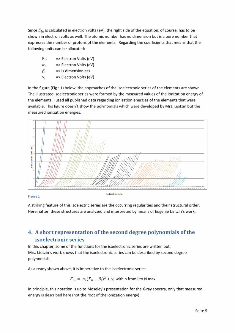
In the figure (Fig.: 1) below, the approaches of the isoelectronic series of the elements are shown.

The illustrated isoelectronic series were formed by the measured values of the ionization energy of

the elements. I used all published data regarding ionization energies of the elements that were

available. This figure doesn’t show the polynomials which were developed by Mrs. Lisitzin but the

measured ionization energies.

Figure 1

A striking feature of this isoelectric series are the occurring regularities and their structural order.

Hereinafter, these structures are analyzed and interpreted by means of Eugenie Lisitzin’s work.

4. A short representation of the second degree polynomials of the

isoelectronic series In this chapter, some of the functions for the isoelectronic series are written out.

Mrs. Lisitzin`s work shows that the isoelectronic series can be described by second degree

polynomials.

As already shown above, it is imperative to the isoelectronic series:

with n from i to N max

In principle, this notation is up to Moseley's presentation for the X-ray spectra, only that measured

energy is described here (not the root of the ionization energy).

0

50

100

150

200

250

300

350

400

1 2 3 4 5 6 7 8 9 10 11 12 13 14 15 16 17 18 19 20 21 22 23 24 25 26 27 28 29 30 31 32 33 34 35 36 37 38 39 40 41 42 43 44 45 46 47 48 49 50 51 52 53 54 55 56 57 58 59 60 61 62 63 64 65 66 67 68 69 70 71 72 73 74 75 76 77 78 79 80 81 82 83 84 85 86 87 88

Seite 6

The first period of the periodic table includes two rows of identical gradient which is expressed by

the coefficient α = 13,6 . This also was determined by Werner Braunbeck. The first isoelectric row is

the hydrogen row and can be written as;

means to be the atomic number of the n-th element. In this row, starts with number one and

ends with the biggest element.

The numerical value of the coefficient corresponds with the ionization energy of the hydrogen atom.

In the case of the hydrogen atom, the parameters β and γ are number zero.

The second row of the first period is the helium series. It starts with the ionization of neutral helium,

with one member less than the hydrogen line. The following represents this series:

So the first two rows of the first period are

fixed.

The second period starts with the lithium series which is the third element of the periodic table.

The essential difference between the rows of the second period is the value of the parameter α of

isoelectric rows. α can be written as

. Starts with the 3rd element and ends –like the other

rows – with the biggest Element.

The fourth row is the isoelectric Beryllium row, where the continuing development of the parameters

goes on.

The parameter α in the second period grows weakly, but noticeable. Regarding and γ there cannot

be made any comment at the moment.

The next series is the isoelectronic series of Bor.

Again the continuing development of the parameters goes on until the end of period two.

The third period begins with the sodium series, the 11th element. The eleventh row is written as:

The following polynomials are characterized by the parameter α which can be written as α

.

The parameters β and γ, however, show the same behavior as in the second period.

In the next section the Moseley diagrams will be described briefly. After that, the parameters α, β

and γ (polynoms of Liszitin) will be described and analyzed regarding their development.

Seite 7

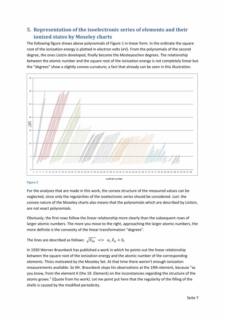
5. Representation of the isoelectronic series of elements and their

ionized states by Moseley charts The following figure shows above polynomials of Figure 1 in linear form. In the ordinate the square

root of the ionization energy is plotted in electron volts (eV). From the polynomials of the second

degree, the ones Listzin developed, finally become the Mosleyeschen degrees. The relationship

between the atomic number and the square root of the ionization energy is not completely linear but

the "degrees" show a slightly convex curvature; a fact that already can be seen in this illustration.

Figure 2

For the analyses that are made in this work, the convex structure of the measured values can be

neglected, since only the regularities of the isoelectronic series should be considered. Just: the

convex nature of the Moseley charts also means that the polynomials which are described by Lisitzin,

are not exact polynomials.

Obviously, the first rows follow the linear relationship more clearly than the subsequent rows of

larger atomic numbers. The more you move to the right, approaching the larger atomic numbers, the

more definite is the convexity of the linear transformation "degrees".

The lines are described as follows:

In 1930 Werner Braunbeck has published a work in which he points out the linear relationship

between the square root of the ionization energy and the atomic number of the corresponding

elements. Thisis motivated by the Moseley Set. At that time there weren’t enough ionization

measurements available. So Mr. Braunbeck stops his observations at the 19th element, because "as

you know, from the element K (the 19. Element) on the inconstancies regarding the structure of the

atoms grows." (Quote from his work). Let me point put here that the regularity of the filling of the

shells is caused by the modified periodicity.

0

5

10

15

20

25

30

35

1 3 5 7 9 11 13 15 17 19 21 23 25 27 29 31 33 35 37 39 41 43 45 47 49 51 53 55 57 59 61 63 65 67 69 71 73 75 77 79 81 83 85 87 89 91 93 95 97 99

Seite 8

So Mr. Braunbeck still assumed that the increase of the degrees within a group is constant. Mrs.

Lisitzin showed that the increase of the paraboles - and this also means the degrees of increases

within a group then - in each group ends at a maximum value.

Furthermore he realized that the performance of ionization energies of the second and third periods

are analog. The first two ionization energies form a subgroup. Apart from this, the six remaining can

be devided elements into two groups. It two threesomes, in which the ionization energy increases;

this refers to the observation of the s and the p sub-shell.

The result of Mr. Braunbeck’s work is that the shielding performances are linear, referred to the

atomic number. From the parallelism of lines, Mr. Braunbeck derives that also the change of the

shielding within one period - referred to the isoeletronic rows - is identical.

Further analyzes are conducted by the Lisitzinschen polynomials, because they describe the really

measured values.

6. Description of the coefficients of the Listzinschen polynomials

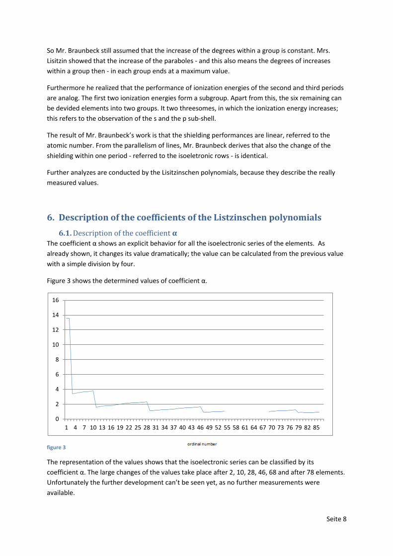
6.1. Description of the coefficient α

The coefficient α shows an explicit behavior for all the isoelectronic series of the elements. As

already shown, it changes its value dramatically; the value can be calculated from the previous value

with a simple division by four.

Figure 3 shows the determined values of coefficient α.

figure 3

The representation of the values shows that the isoelectronic series can be classified by its

coefficient α. The large changes of the values take place after 2, 10, 28, 46, 68 and after 78 elements.

Unfortunately the further development can’t be seen yet, as no further measurements were

available.

0

2

4

6

8

10

12

14

16

1 4 7 10 13 16 19 22 25 28 31 34 37 40 43 46 49 52 55 58 61 64 67 70 73 76 79 82 85

Seite 9

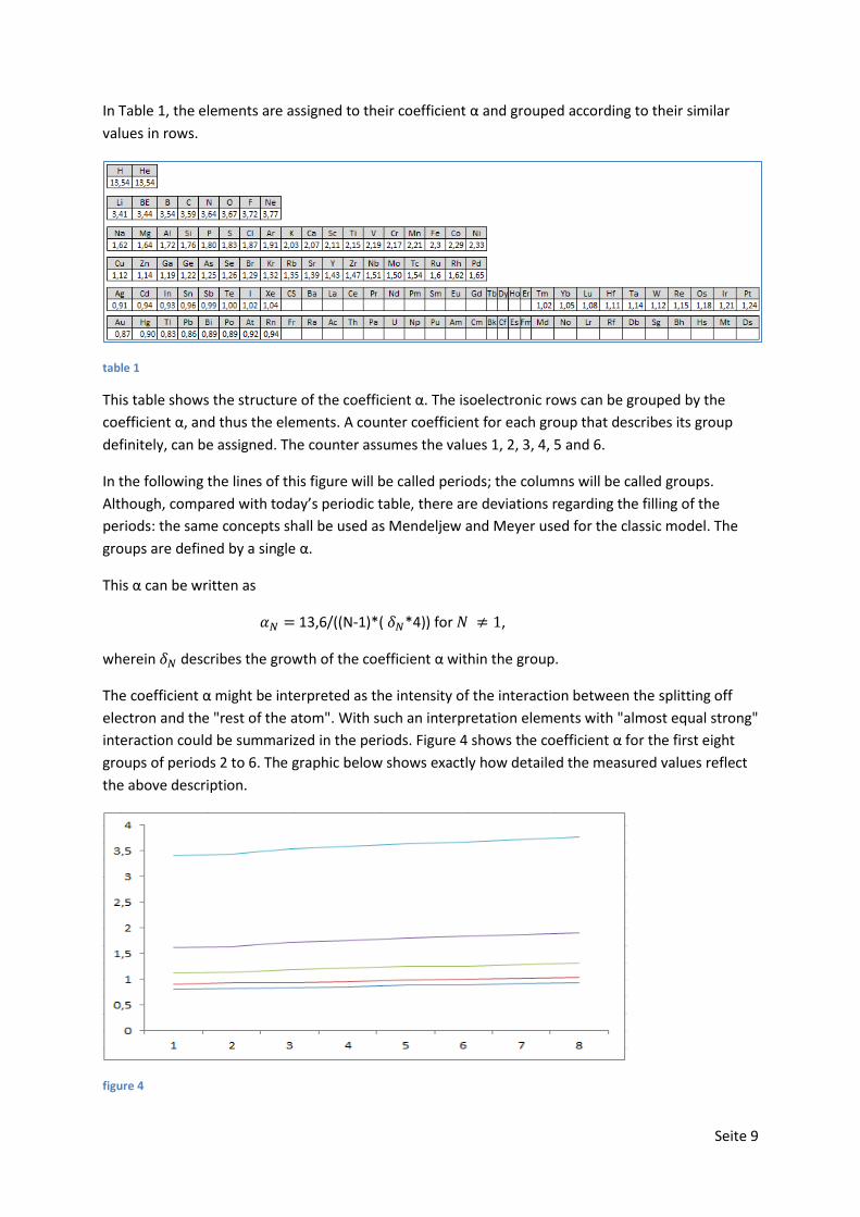
In Table 1, the elements are assigned to their coefficient α and grouped according to their similar

values in rows.

table 1

This table shows the structure of the coefficient α. The isoelectronic rows can be grouped by the

coefficient α, and thus the elements. A counter coefficient for each group that describes its group

definitely, can be assigned. The counter assumes the values 1, 2, 3, 4, 5 and 6.

In the following the lines of this figure will be called periods; the columns will be called groups.

Although, compared with today’s periodic table, there are deviations regarding the filling of the

periods: the same concepts shall be used as Mendeljew and Meyer used for the classic model. The

groups are defined by a single α.

This α can be written as

13,6/((N-1)*( *4)) for ,

wherein describes the growth of the coefficient α within the group.

The coefficient α might be interpreted as the intensity of the interaction between the splitting off

electron and the "rest of the atom". With such an interpretation elements with "almost equal strong"

interaction could be summarized in the periods. Figure 4 shows the coefficient α for the first eight

groups of periods 2 to 6. The graphic below shows exactly how detailed the measured values reflect

the above description.

figure 4

Seite 10

The top line shows the coefficients α of the second period. The line directly below reflects the third

period. The remaining three lines represent the coefficient α of the periods four, five and six. To

make the chart as readable as possible, there is no further scaling in it.

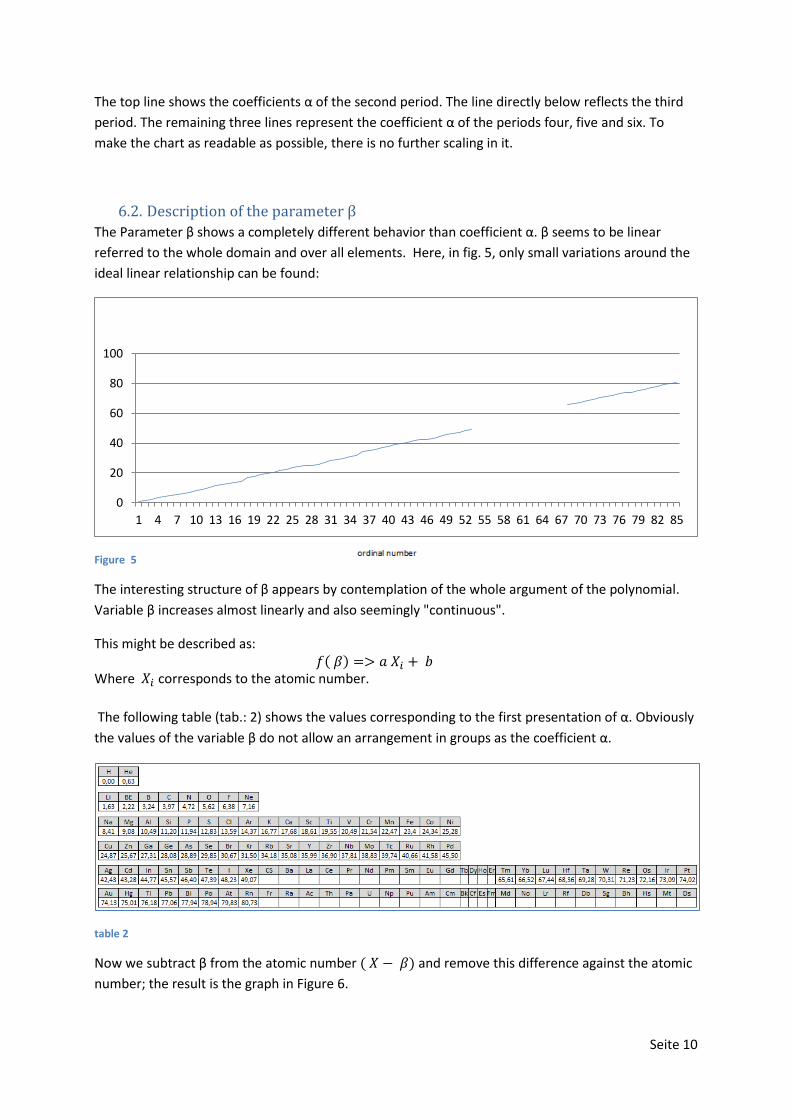
6.2. Description of the parameter β

The Parameter β shows a completely different behavior than coefficient α. β seems to be linear

referred to the whole domain and over all elements. Here, in fig. 5, only small variations around the

ideal linear relationship can be found:

Figure 5

The interesting structure of β appears by contemplation of the whole argument of the polynomial.

Variable β increases almost linearly and also seemingly "continuous".

This might be described as: Where corresponds to the atomic number.

The following table (tab.: 2) shows the values corresponding to the first presentation of α. Obviously

the values of the variable β do not allow an arrangement in groups as the coefficient α.

table 2

Now we subtract β from the atomic number and remove this difference against the atomic

number; the result is the graph in Figure 6.

0

20

40

60

80

100

1 4 7 10 13 16 19 22 25 28 31 34 37 40 43 46 49 52 55 58 61 64 67 70 73 76 79 82 85

Seite 11

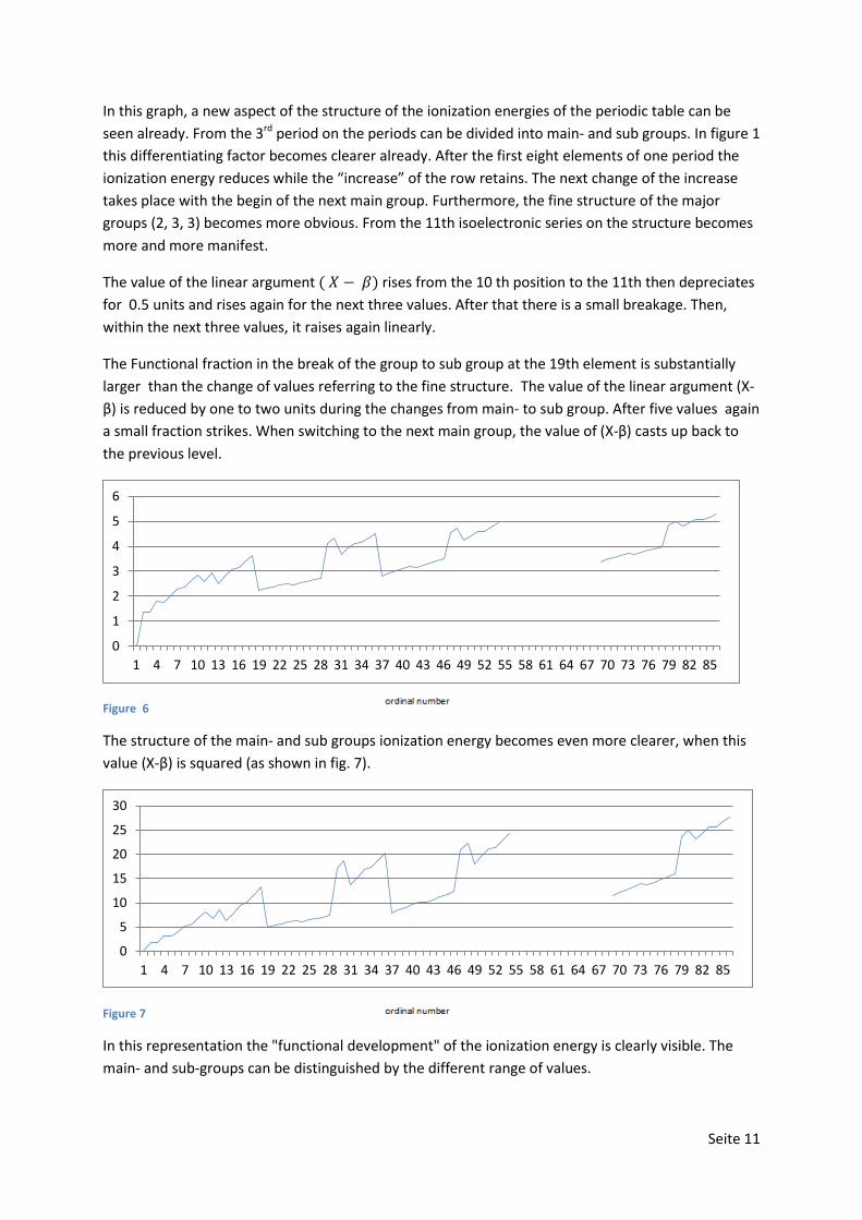
In this graph, a new aspect of the structure of the ionization energies of the periodic table can be

seen already. From the 3rd period on the periods can be divided into main- and sub groups. In figure 1

this differentiating factor becomes clearer already. After the first eight elements of one period the

ionization energy reduces while the “increase” of the row retains. The next change of the increase

takes place with the begin of the next main group. Furthermore, the fine structure of the major

groups (2, 3, 3) becomes more obvious. From the 11th isoelectronic series on the structure becomes

more and more manifest.

The value of the linear argument rises from the 10 th position to the 11th then depreciates

for 0.5 units and rises again for the next three values. After that there is a small breakage. Then,

within the next three values, it raises again linearly.

The Functional fraction in the break of the group to sub group at the 19th element is substantially

larger than the change of values referring to the fine structure. The value of the linear argument (X-

β) is reduced by one to two units during the changes from main- to sub group. After five values again

a small fraction strikes. When switching to the next main group, the value of (X-β) casts up back to

the previous level.

Figure 6

The structure of the main- and sub groups ionization energy becomes even more clearer, when this

value (X-β) is squared (as shown in fig. 7).

Figure 7

In this representation the "functional development" of the ionization energy is clearly visible. The

main- and sub-groups can be distinguished by the different range of values.

0

1

2

3

4

5

6

1 4 7 10 13 16 19 22 25 28 31 34 37 40 43 46 49 52 55 58 61 64 67 70 73 76 79 82 85

0

5

10

15

20

25

30

1 4 7 10 13 16 19 22 25 28 31 34 37 40 43 46 49 52 55 58 61 64 67 70 73 76 79 82 85

Seite 12

It seems as if the real structure does not begin before the third period. But also in the area of the

second period the fine structures are already visible.

In various publications, β is interpreted as a screening constant. It protects the attractive forces

against the final flaking electron. This protection shield is formed by the remaining electrons; in

other words: The shielding is formed by electrons.

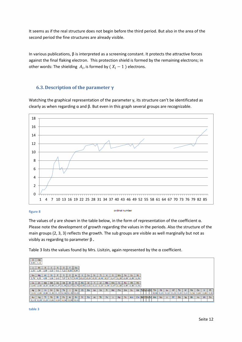
6.3. Description of the parameter γ

Watching the graphical representation of the parameter γ, its structure can’t be identificated as

clearly as when regarding α and β. But even in this graph several groups are recognizable.

figure 8

The values of γ are shown in the table below, in the form of representation of the coefficient α.

Please note the development of growth regarding the values in the periods. Also the structure of the

main groups (2, 3, 3) reflects the growth. The sub groups are visible as well marginally but not as

visibly as regarding to parameter β .

Table 3 lists the values found by Mrs. Lisitzin, again represented by the α coefficient.

table 3

0

2

4

6

8

10

12

14

16

18

1 4 7 10 13 16 19 22 25 28 31 34 37 40 43 46 49 52 55 58 61 64 67 70 73 76 79 82 85

Seite 13

In some public works it is tried to interpret γ as a parameter of interaction of the electronic

repulsion.

7. Description of the isoelectronic series

As shown in Figure 1, the isoelectronic series are subject to certain regularities which can be

described by formulas and numbers.

What strikes in Figure 1 first is that the gradients of the rows from left to right decrease . The

decrease happens within the groups. Within these groups, the rows drift nearly parallel. Only at

those positions in the periodic table where the switch between main and side groups takes place, the

initial value of the isoelectronic series falls; parameter β reflects that. . Furthermore, the structure of

the ionization energy in ground state continues in each section. That means that the ionization

energies of the elements and their ionized states change consistently in solid proportions to each

other.

The first group of isoelectronic series contains of two rows, the second group eight rows, the third

and fourth group each contains 18 rows, and finally the fifth and sixth group each contain 32

isoelectronic rows.

As shown before, the gradient of a following group corresponds to a quarter of the previous group.

Within each group the gradient of each row rises from left to right. From the second group on, the

fine structure 2, 3, 3 of the isoelectronic series can be seen at the start of each pitch group. After

these eighth groups, a secondary group follows and it is the one with the same gradient but also with

a gap on a value basis. It is parameter β that describes that gap. Not before that the next group, with

a reduced gradient, follows.

The first group contains 1 * 2 rows.

The second group contains 1 * 2 and 3 * 2 rows.

The third and fourth group contains 1 * 2 and 3 * 2 and 5 * 2 rows.

The fifth and sixth group contains 1 * 2 and 3 * 2 and 5 * 2 and 7 * 2 rows.

It needs to be investigated whether any rule could be discharged from that . It strikes that the

increase of elements in each period is odd and even again by the multiplication with two.

8. Implortance of the found properties of the isoelectronic series

referred to the Periodic Table By the current state of scientific knowledge in today's presentation of the periodic table the

elements are lined up according to their atomic number. The periodicity of the elements is justified

by their chemical properties. Each period begins with an alkali metal which contains only one valence

electron and is consequently monovalent. Each period ends with a noble gas. Noble gases own a

completed outer shell and therefore are chemically inert. The first period is an exception, it does not

start with an alkali metal but with the element hydrogen.

Seite 14

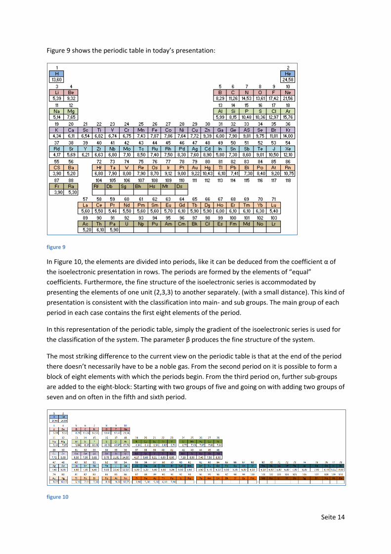
Figure 9 shows the periodic table in today’s presentation:

figure 9

In Figure 10, the elements are divided into periods, like it can be deduced from the coefficient α of

the isoelectronic presentation in rows. The periods are formed by the elements of “equal”

coefficients. Furthermore, the fine structure of the isoelectronic series is accommodated by

presenting the elements of one unit (2,3,3) to another separately. (with a small distance). This kind of

presentation is consistent with the classification into main- and sub groups. The main group of each

period in each case contains the first eight elements of the period.

In this representation of the periodic table, simply the gradient of the isoelectronic series is used for

the classification of the system. The parameter β produces the fine structure of the system.

The most striking difference to the current view on the periodic table is that at the end of the period

there doesn’t necessarily have to be a noble gas. From the second period on it is possible to form a

block of eight elements with which the periods begin. From the third period on, further sub-groups

are added to the eight-block: Starting with two groups of five and going on with adding two groups of

seven and on often in the fifth and sixth period.

figure 10

Seite 15

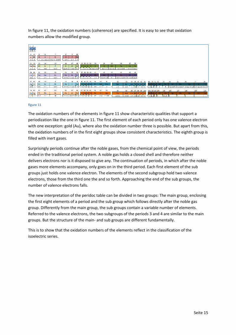
In figure 11, the oxidation numbers (coherence) are specified. It is easy to see that oxidation

numbers allow the modified group.

figure 11

The oxidation numbers of the elements in figure 11 show characteristic qualities that support a

periodization like the one in figure 11. The first element of each period only has one valence electron

with one exception: gold (Au), where also the oxidation number three is possible. But apart from this,

the oxidation numbers of in the first eight groups show consistent characteristics. The eighth group is

filled with inert gases.

Surprisingly periods continue after the noble gases, from the chemical point of view, the periods

ended in the traditional period system. A noble gas holds a closed shell and therefore neither

delivers electrons nor is it disposed to give any. The continuation of periods, in which after the noble

gases more elements accompany, only goes on in the third period. Each first element of the sub

groups just holds one valence electron. The elements of the second subgroup hold two valence

electrons, those from the third one the and so forth. Approaching the end of the sub groups, the

number of valence electrons falls.

The new interpretation of the peridoc table can be divided in two groups: The main group, enclosing

the first eight elements of a period and the sub group which follows directly after the noble gas

group. Differently from the main group, the sub groups contain a variable number of elements.

Referred to the valence electrons, the two subgroups of the periods 3 and 4 are similar to the main

groups. But the structure of the main- and sub groups are different fundamentally.

This is to show that the oxidation numbers of the elements reflect in the classification of the

isoelectric series.

Seite 16

9. Application of the discovered periodicity to the quantum-

mechanical shell model Another order for the structure of the elements is the quantum-mechanical shell model. The atomic

shells are characterized by the four quantum numbers: main quantum number (N), the angular

momentum quantum number (l), the magnetic quantum number (m) and the spin (± 1/2). According

to the Pauli principle the four quantum numbers must vary in minimum one quantum value in each

quantum mechanical system, i.e. that a state can always only be occupied by one electron.

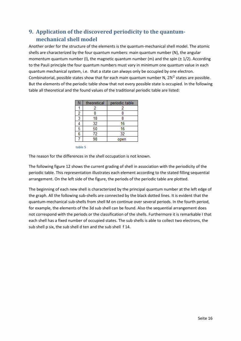
Combinatorial, possible states show that for each main quantum number N, states are possible.

But the elements of the periodic table show that not every possible state is occupied. In the following

table all theoretical and the found values of the traditional periodic table are listed:

The reason for the differences in the shell occupation is not known.

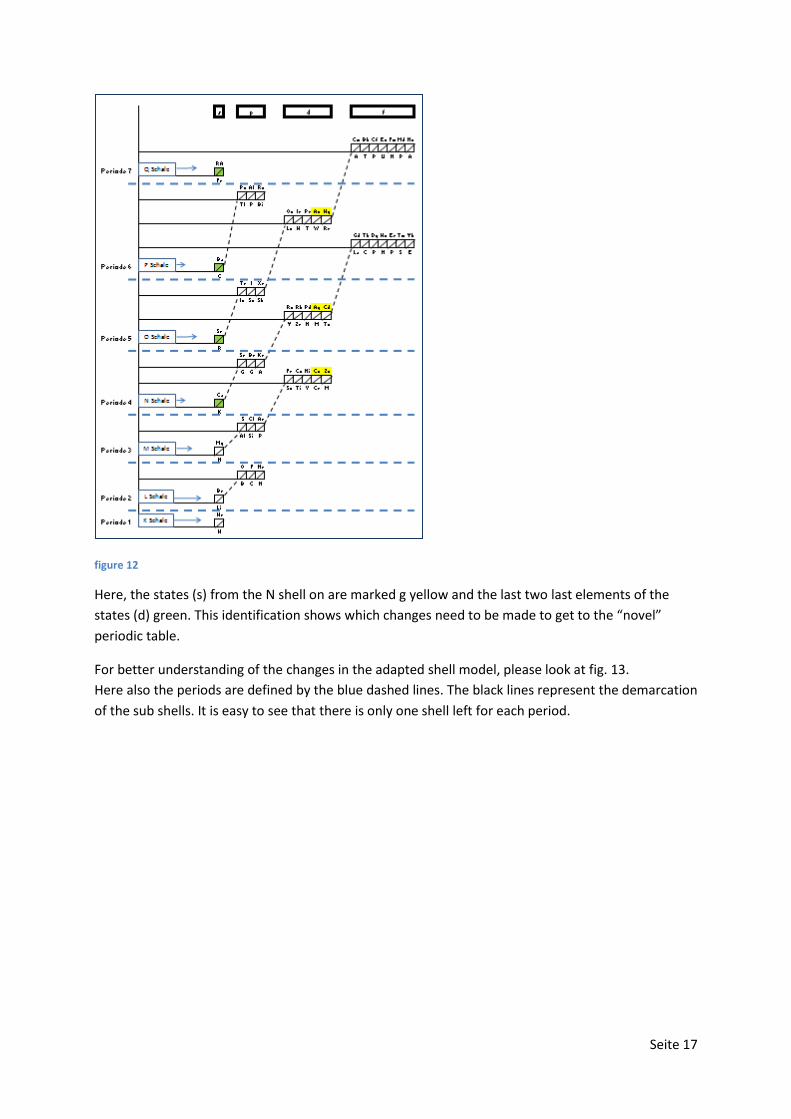
The following figure 12 shows the current grading of shell in association with the periodicity of the

periodic table. This representation illustrates each element according to the stated filling sequential

arrangement. On the left side of the figure, the periods of the periodic table are plotted.

The beginning of each new shell is characterized by the principal quantum number at the left edge of

the graph. All the following sub-shells are connected by the black dotted lines. It is evident that the

quantum-mechanical sub-shells from shell M on continue over several periods. In the fourth period,

for example, the elements of the 3d sub shell can be found. Also the sequential arrangement does

not correspond with the periods or the classification of the shells. Furthermore it is remarkable I that

each shell has a fixed number of occupied states. The sub shells is able to collect two electrons, the

sub shell p six, the sub shell d ten and the sub shell f 14.

table 5

Seite 17

figure 12

Here, the states (s) from the N shell on are marked g yellow and the last two last elements of the

states (d) green. This identification shows which changes need to be made to get to the “novel”

periodic table.

For better understanding of the changes in the adapted shell model, please look at fig. 13.

Here also the periods are defined by the blue dashed lines. The black lines represent the demarcation

of the sub shells. It is easy to see that there is only one shell left for each period.

Seite 18

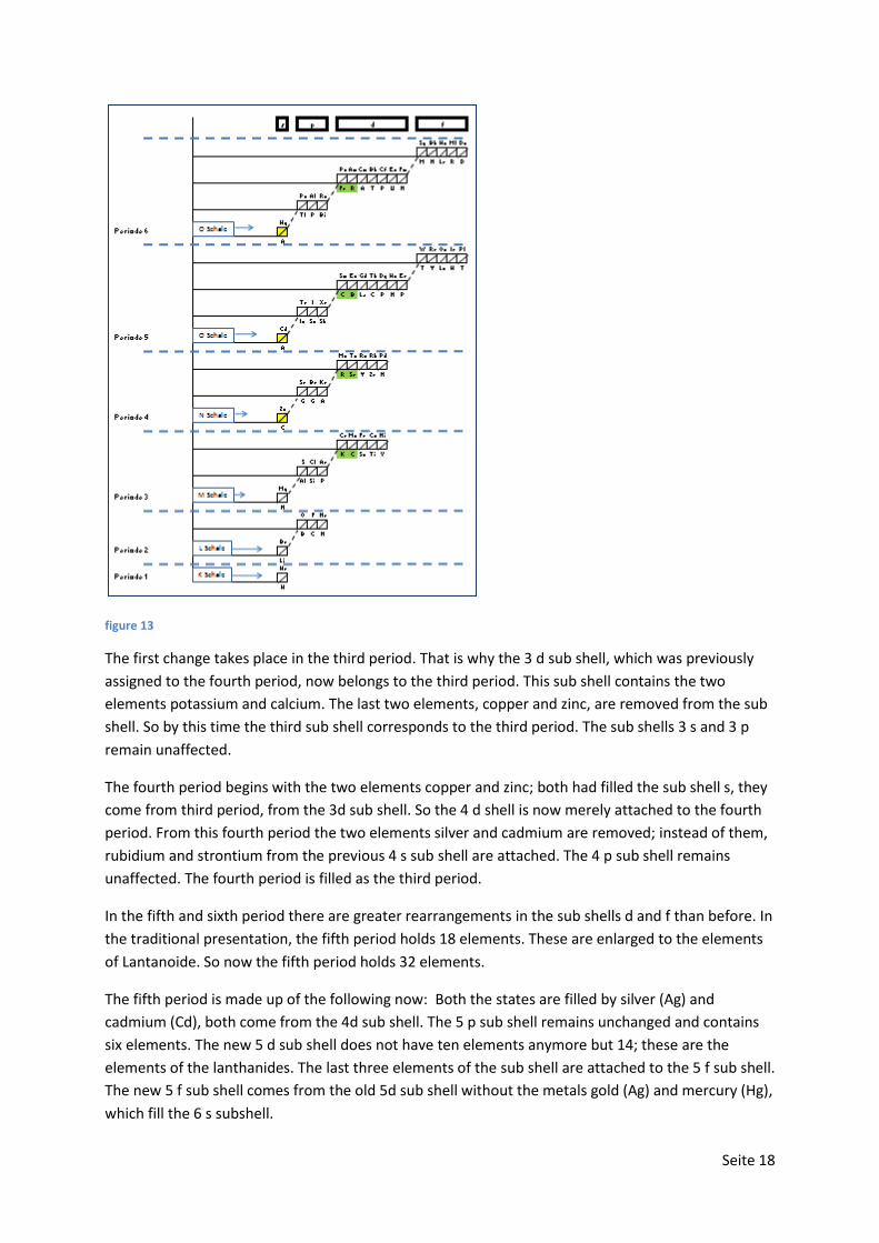
figure 13

The first change takes place in the third period. That is why the 3 d sub shell, which was previously

assigned to the fourth period, now belongs to the third period. This sub shell contains the two

elements potassium and calcium. The last two elements, copper and zinc, are removed from the sub

shell. So by this time the third sub shell corresponds to the third period. The sub shells 3 s and 3 p

remain unaffected.

The fourth period begins with the two elements copper and zinc; both had filled the sub shell s, they

come from third period, from the 3d sub shell. So the 4 d shell is now merely attached to the fourth

period. From this fourth period the two elements silver and cadmium are removed; instead of them,

rubidium and strontium from the previous 4 s sub shell are attached. The 4 p sub shell remains

unaffected. The fourth period is filled as the third period.

In the fifth and sixth period there are greater rearrangements in the sub shells d and f than before. In

the traditional presentation, the fifth period holds 18 elements. These are enlarged to the elements

of Lantanoide. So now the fifth period holds 32 elements.

The fifth period is made up of the following now: Both the states are filled by silver (Ag) and

cadmium (Cd), both come from the 4d sub shell. The 5 p sub shell remains unchanged and contains

six elements. The new 5 d sub shell does not have ten elements anymore but 14; these are the

elements of the lanthanides. The last three elements of the sub shell are attached to the 5 f sub shell.

The new 5 f sub shell comes from the old 5d sub shell without the metals gold (Ag) and mercury (Hg),

which fill the 6 s subshell.

Seite 19

In the sixth period, there have been similar changes like in the fifth. Here, the two 6 s states are

occupied by gold and mercury. The 6 p sub shell remains, as in other periods, unaffected. The new 6

d sub shell contains, like the 5 d sub shell, now 14 elements. The sub-group of actinides is assigned

the 5 d sub shell. This sub-group of actinides is again enlarged by the two elements of the 7 s state:

francium (Fr) and radium (Rd). At the end of this sub shell both the two elements Mendelevium (Md)

and nobelium (No) are missed. The 6 f sub shell completes and closes the 6th period and ends with

the 110th element.

The seventh period starts with the 111th element, which is Roentgenium (Rg), the second element in

the s 7 sub shell is Copernicium (Co).

At this point we are already deep going into the subject of artificially produced elements and for this

reason I interrupt the description of changes in the shell model here. The filling of the further shells

will continue as described.

10. Scientific application of the periodicity found to the extended

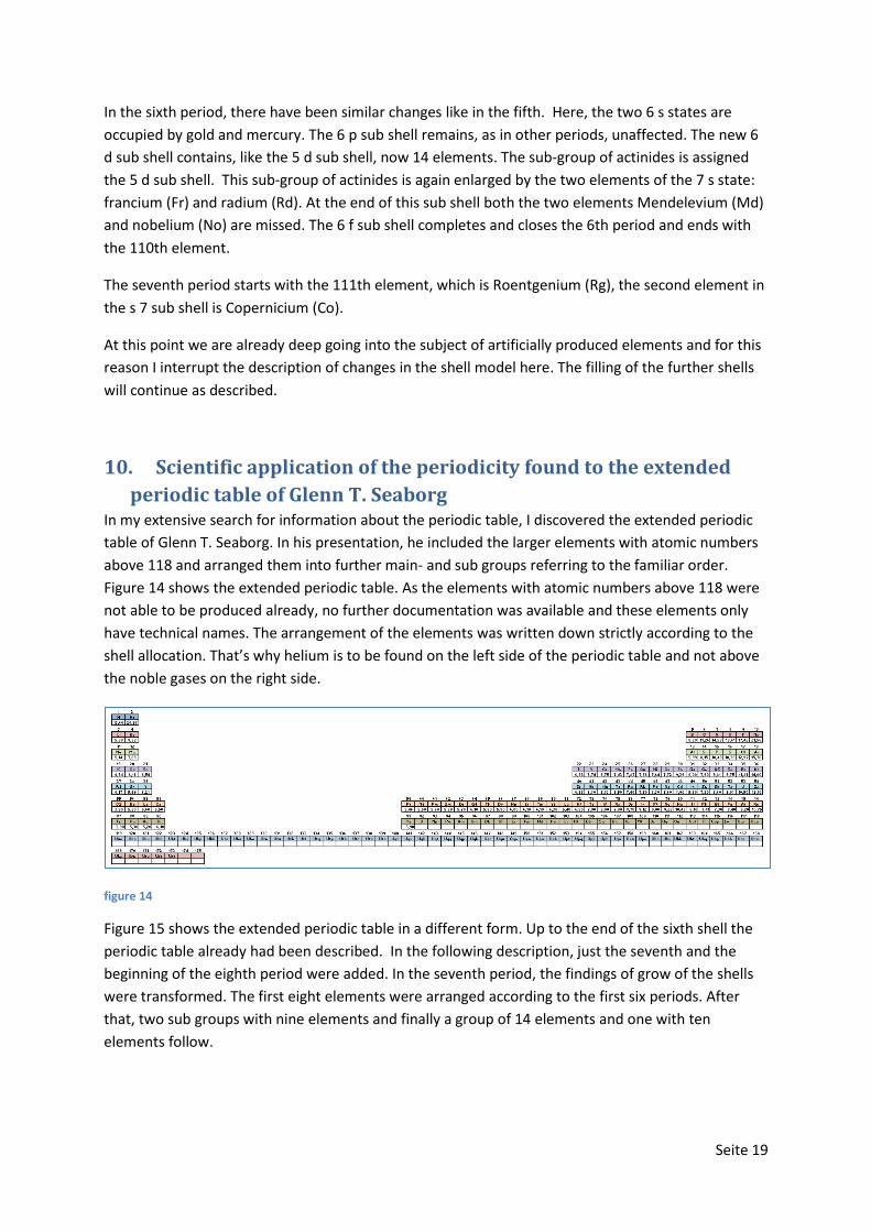
periodic table of Glenn T. Seaborg In my extensive search for information about the periodic table, I discovered the extended periodic

table of Glenn T. Seaborg. In his presentation, he included the larger elements with atomic numbers

above 118 and arranged them into further main- and sub groups referring to the familiar order.

Figure 14 shows the extended periodic table. As the elements with atomic numbers above 118 were

not able to be produced already, no further documentation was available and these elements only

have technical names. The arrangement of the elements was written down strictly according to the

shell allocation. That’s why helium is to be found on the left side of the periodic table and not above

the noble gases on the right side.

figure 14

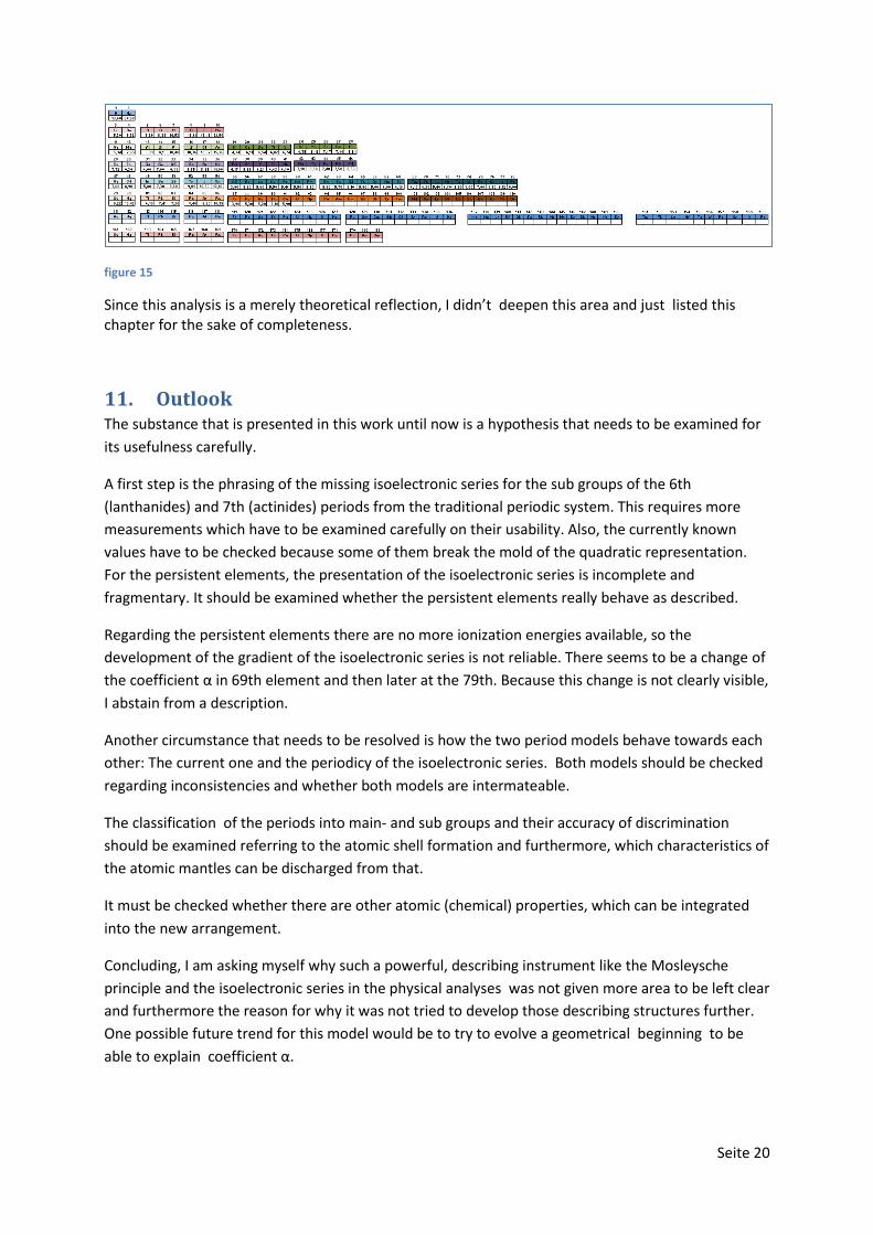
Figure 15 shows the extended periodic table in a different form. Up to the end of the sixth shell the

periodic table already had been described. In the following description, just the seventh and the

beginning of the eighth period were added. In the seventh period, the findings of grow of the shells

were transformed. The first eight elements were arranged according to the first six periods. After

that, two sub groups with nine elements and finally a group of 14 elements and one with ten

elements follow.

Seite 20

figure 15

Since this analysis is a merely theoretical reflection, I didn’t deepen this area and just listed this chapter for the sake of completeness.

11. Outlook The substance that is presented in this work until now is a hypothesis that needs to be examined for

its usefulness carefully.

A first step is the phrasing of the missing isoelectronic series for the sub groups of the 6th

(lanthanides) and 7th (actinides) periods from the traditional periodic system. This requires more

measurements which have to be examined carefully on their usability. Also, the currently known

values have to be checked because some of them break the mold of the quadratic representation.

For the persistent elements, the presentation of the isoelectronic series is incomplete and

fragmentary. It should be examined whether the persistent elements really behave as described.

Regarding the persistent elements there are no more ionization energies available, so the

development of the gradient of the isoelectronic series is not reliable. There seems to be a change of

the coefficient α in 69th element and then later at the 79th. Because this change is not clearly visible,

I abstain from a description.

Another circumstance that needs to be resolved is how the two period models behave towards each

other: The current one and the periodicy of the isoelectronic series. Both models should be checked

regarding inconsistencies and whether both models are intermateable.

The classification of the periods into main- and sub groups and their accuracy of discrimination

should be examined referring to the atomic shell formation and furthermore, which characteristics of

the atomic mantles can be discharged from that.

It must be checked whether there are other atomic (chemical) properties, which can be integrated

into the new arrangement.

Concluding, I am asking myself why such a powerful, describing instrument like the Mosleysche

principle and the isoelectronic series in the physical analyses was not given more area to be left clear

and furthermore the reason for why it was not tried to develop those describing structures further.

One possible future trend for this model would be to try to evolve a geometrical beginning to be

able to explain coefficient α.

Seite 21

12. Sources Textbooks:

Ingolf V. Hertel und C.-P. Schulz

Atome, Moleküle und optische Physik 1 + 2; Springerverlag Berlin Heidelberg 2010

Herbert Graewe

Atomphysik

Aulis Verlag deubner & Co KG 1979

Haken und Wolf

Atom und Quantenphysik

Springerverlag Berlin Heidelberg 1987

Measurement results:

Ionisationsenergien:

Bashkin S. / Stoner J.O. , jr(1975, 1981, 1982)

Atomic energie leves and grotian diagrams; Band 1+2+3+4

North-Holland Publishing Company Düsseldorf, New York, London

National Institute of Standards and Technology

Internet:

http://www.nist.gov/pml/data/periodic.cfm

Oxydationszahlen:

Wikipedia

http://de.wikipedia.org/wiki/Liste_der_Oxidationsstufen_der_chemischen_Elemente

Original works:

H.G.J. Moseley

The High-Frequency Spectra oft he Elements

Phil. Mag. 1913 (p.1024)

Eugenie Lisitzin

Über die Ionisierungsspannungen der Elemente in verschiedenen Ionisierungszuständen; Societas

Scientiarum Fennica COMMENTATIONES PHYSICO – MATHEMATICAE. X. 4.

Werner Braunbek

Die Moseleydiagramme der Ionisierungsspannungen der leichten Atome und Ionen

Springer Verlag (Eingegangen am 13 Mai 1930)

publicly available:

Erweitertes Periodensystem

Harry H. Binder

Die Grenzen des Periodensystems der Elemente

LINK:

http://de.wikipedia.org/wiki/Erweitertes_Periodensystem