Journal of Research of the National Bureau of Standards

Description of the Thermotropic Behavior Of Membrane Bilayers

In Terms of Raman Spectral Parameters: A Two-State Model

Volume 92 Number 2 March-April 1987

William H. Kirchhoff

National Bureau of Standards Gaithersburg, MD 20899

Ira W. Levin

National Institutes of Health Bethesda, MD 20205

An analytical expression is developed for describing the thermotropic behav­ior of membrane bilayers as studied by Raman spectroscopy. The expression is derived from a two-state model of the main gel to liquid crystalline phase transition in lipid bilayers. Experimen­tal data for a variety of diacylphos­phatidylcholines and their derivatives have been fit by least squares to the two-state expression to within cur­rently achievable measurement error. Numerical techniques have been de­veloped for placing bounds on the

parameters of the two-state model in situations of sparse data in the phase transition region. By fitting the model to the measured spectroscopic data, es­timates of the extent of cooperativity in the phase transition can be obtained in a systematic manner.

Key words: logistic function; mem­brane; phase transition; Raman spec­troscopy; two-state model.

Accepted: December 3, 1986

Introduction

In recent years the use of Raman spectroscopy for the study of the phase transition and the order/ disorder behavior of both intact and reconstituted membrane bilayers has gained dramatically in pop­ularity through the wide range of applications amenable to spectroscopic techniques [1]1. Al­though calorimetric measurements can provide ac­curate information on enthalpy changes that occur during phase transitions, they provide little insight into the nature of the molecular reorganization ac­companying the phase transition. Since Raman spectra are particularly sensitive to the conforma­tional, packing, and dynamical changes involving

About the Authors: William H. Kirchhoff is with the NBS Center for Chemical Physics. Ira W. Levin is with the Laboratory of Chemical Physics in the National Institute of Arthritis, Diabetes, and Digestive and Kidney Diseases, NIH.

(Figures in brackets indicate literature references.

113

the hydrocarbon chains, bilayer reorganizations within, for example, the hydrophobic region of the membrane, may be monitored directly as a function of temperature. These observations can be made in an aqueous medium, without either the introduc­tion of bulky molecular probes or elaborate sample preparation. By using low laser excitation powers (15-200 m W) at the sample, external perturbations to the system are minimized. Because of the sensi­tivity of the spectra to conformational changes, Ra­man spectroscopy has also been useful in elucidating the effects of intrinsic and peripheral components such as sterols and proteins on the thermal properties of membranes. In a few systems, reconstituted, naturally-occurring membranes have been studied and have provided useful information obtainable only from spectroscopic examination [2].

Although the vibrational assignments for the spectra of lipid bilayers are complex, they are un­derstood sufficiently well to allow discussion of

Journal of Research of the National Bureau of Standards

membrane reorganizations in terms of the observed spectroscopic frequencies, intensities and line­widths of a variety of spectral features reflecting the head group, interface, and acyl chain regions of the lipid components. A particularly useful ap­proach for presenting the thermal data has been in terms of spectral peak height intensity ratios deter­mined from either the 2900 cm- I carbon-hydrogen or 1100 cm -I carbon-carbon stretching mode re­gions. In general, these data are primarily sensitive either to alterations in the lateral interactions or to intermolecular order of the acyl chains and intra­chain trans-gauche conformational changes, respec­tively.

In this paper we propose an analytical expres­sion, based upon a two-state model of the primary phase transition phenomenon, which is useful for systematical1y describing the form of the tempera­ture profiles. We also describe an approach, based on a nonlinear, least squares analysis, for extracting relevant thermodynamic information from the tem­perature dependence of the observed spectra. This approach is robust in handling the range of data encountered in studies of membrane phase transi­tions.

Thermodynamic Model

Within the last 10 years a number of models have appeared describing within either a thermody­namic or statistical mechanical framework various features of the main phase transition in membrane bilayers. Most of these models have been critically reviewed by Nagle [3]. An additional review by Israelachvili, et aI. [4] discusses the physical princi­ples of membrane organization and includes de­scriptions of membrane-protein interactions and nonbilayer lipid structures. We concern ourselves here with the simplest of these phase transition models; namely, that of thermodynamic equi­librium between noninteracting domains in either one of two states [5]. We have been guided by the philosophy that the accuracy with which a simple model can quantitatively describe the experimental data serves as a guide to assessing the required fea­tures of a more complex model, to comparing and evaluating two or more models, and to defining the accuracy requirements of additional measurements.

The derivation of the thermodynamic model is presented in Appendix A in detail in order to dis­tinguish clearly between numbers of molecules and numbers of domains in each of the two states since the observed spectral intensities are determined by the number of molecules in each of the states while

114

the temperature dependence of the spectral intensi­ties is determined by the distribution of domain sizes. The mathematical development follows closely the description by Hill of the two-state model for small systems [6]. The resulting analyti­cal expression for the temperature dependence of the Raman spectra are identical to those published by Dluhy, et al. [7] using the Zimm-Bragg theory originally developed for describing polypeptide de­naturation [8]. The difference between the thermo­dynamic and the Zimm-Bragg developments is in the interpretation of the parameters derived from the analysis. We prefer the thermodynamic devel­opment because of the simplicity of its physical in­terpretation. For so long as the data are described by a simple model, it seems little more than a mat­ter of taste as to how the parameters are to be inter­preted. Only when the data can be seen to contain additional information would it be fruitful to apply a more complex model. Finally, though the deriva­tion is applied in this paper to Raman spectroscopic data, it is generally applicable to all spectroscopic studies of such cooperative phenomena.

In the two-state model, a single bilayer is consid­ered to consist of domains of varying numbers of lipid molecules n with each domain existing in one of two states labeled A and B. The distribution of domain sizes and the requirement that all molecules within a domain exist either in state A (the low­temperature gel state) or in state B (the high-tem­perature liquid crystalline state) determine the cooperativity exhibited by the bilayers during the phase transition between the two states. The distri­bution of domain sizes is assumed to be tempera­ture independent, while the number of domains in either state is temperature dependent. Although a phase transition in the strictest sense is excluded for a distribution of domains of finite size, the discon­tinuous nature of the phase transition will be ap­proximated for large values of n.

The temperature dependence of the intensity I v of a spectral feature (Raman or otherwise) that de­pends upon the distribution between two states of the molecules being observed is given by eq (A32) in Appendix A:

(1)

The dimensionless, reduced temperature t is de­fined as t = (T - To)/ D, where To is the midpoint of the phase transition and the scale factor D is related to the enthalpy of transition per mole of lipid molecules, W, and the effective domain size, neff, by:

Journal of Research of the National Bureau of Standards

D = (RTJ)/ t:Jineff (2)

As discussed in Appendix A, eq (1) represents an approximation to a summation over a distribution of domain sizes. To test the accuracy of this ap­proximation, sets of hypothetical data were created using a lognormal distribution [9] of domain sizes from which Raman intensities were calculated for values of NA and N B , the numbers of molecules in states A and B respectively. The values of NA and NB were calculated for the lognormal distribution using eqs (A21) and (A24). The lognormal distribu­tion was chosen because it excludes domains of negative size and allows for a pronounced skewing to high values of n. This skewing causes various measures of the center of the distribution to differ significantly and provides a sensitive test of a sin­gle-term approximation to a sum over a distribu­tion. The data sets corresponded to distributions of varying breadth which, when fit by the method of least squares to eq (1), gave the same value of neff.

In table 1, five measures of the center of a distri­bution: the mode, M, which is the most populous value of n, the mean value of n, < n >, the root mean square of n, v' <n2>, the median, n(50%), and the value of <n2>/ <n > are compared with the value of neff returned by the least squares fit for three distributions of varying spread. It can be seen that as the spread of the distribution narrows, the agreement of all of these measures improves. Even

Table 1. Comparison of a single term fit to three distributions.

Distribution Parameters

Mode

Range in n a

<n>

1-11,679

36.3

median 117

Least Squares Fit neff 100 to Eq 1

2.1%

to Eq 3 136.2

s 1.0%

0.46%

30 90

1-3,963 21-387

79.2 98.2

109.5 101.0

151.3 104.0

110 101

100 100

1.2% 0.2%

113 101

0.8% 0.2%

0.24% 0.02%

-Range: values of n for which the population> 10- 8 x population of mode.

bS : relative (to the value of A-B) standard deviation of the least squares fit.

cslope: value of baseline slope relative to the value of A-B.

115

though, for the broadest distribution, the values of these measures covered more than an order of magnitude, eq (1) gave a satisfactory fit with a rela­tive standard deviation of 2%.

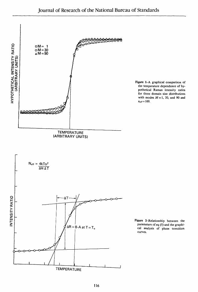
Other conclusions may be drawn from the data presented in table 1. The value of neff obtained from the least squares fit was best approximated by the root mean square value v' <n2>, and the median, n(50%), rather than by <n2>/ <n > as we had initially expected. This is a function, however, of the density of data in the vicinity of the transition interval. If the data range is narrowed to include only the transition interval and if the number of data in that region is increased, then the limit of <n2>/ <n > is approached in agreement with the observation in Appendix A that this measure gives the correct temperature dependence at the asymp­totes and at the inflection point when used in a single term approximation to the sum over domain sizes. Another pronounced effect of the spread of the distribution was to give a more gradual conver­gence to the asymptotic limits and thus, the appear­ance of sloping rather than horizontal asymptotes. This can be seen in figure 1 in which the hypothet­ical intensity ratio profiles are drawn for each of the three distributions listed in table 1. The sloping asymptotes arise from contributions from domains of small size as originally suggested by Sturtevant [10].

A somewhat better fit to broad distributions can be obtained by modifying eq (1) in order to allow for nonhorizontal asymptotes, namely:

Iv IAv+Iav{T - To) + IBv+Ibv(T - To) (1 +e') (1 +e-')

(3)

From table 1 it can be seen that inclusion of a nonhorizontal baseline in the fit of the hypothetical data improved the quality of the fit, as judged by the standard deviation, and increased the estimate of the value ofn slightly, though not nearly enough to bring it to its expected value of <n2>/ <n >.

In the absence of an analytical expression such as eq (3), it has been customary to estimate To and the van't Hoff enthalpies from observed temperature profiles using straight line approximations to the three distinct regions of the profiles. Thus, flT has been defined as the temperature interval between the intersection of a line drawn tangent to the phase transition curve at its inflection point and the two lines drawn tangent to the high and low tem­perature asymptotes. This definition of flT is illus­trated in figure 2. The relationship of AT to the scale parameter D of eq (3) can be calculated di­rectly to give AT=4D, ignoring terms of order

o ~ ~ a: >­t: en 2 w .... ~

Journal of Research of the National Bureau of Standards

oM= 1 oM=30 ~M=90

Nell = 4kTo2

.1H .1 T

TEMPERATURE (ARBITRARY UNITS)

TEMPERATURE

116

Figure I-A graphical comparison of the temperature dependence of hy­pothetical Raman intensity ratios for three domain size distributions with modes M = I, 30, and 90 and n.rr= 100.

Figure 2-Relationship between the parameters of eq (5) and the graphi­cal analysis of phase transition curves.

Journal of Research of the National Bureau of Standards

(lbv-Iav)l(IBv-1Av). From the definition of D given by eq (2),

(4)

Comparison of eq (4) with similar expressions given by Sturtevant [11] indicates that AT corre­sponds to the AT used for calorimetric determina­tions of van't Hoff enthalpies. Care should be taken in the interpretation of neff' however, since esti­mates of the slope made as close to the inflection point as possible will give values of neff approach­ing <n2>1 <n > which, for broad distributions of domain sizes, can be an order of magnitude higher than <n >.

In the Raman spectroscopic experiment tempera­ture profiles are collected over periods of several hours. Since fluctuations in the intensity of the inci­dent laser radiation lead to corresponding fluctua­tions in the observed Raman intensities, the ratio of the intensities of two spectral features at different scattering frequencies provides a more precisely defined temperature profile which is relatively in­dependent of the experimental environment. More­over, if the vibrational features are chosen to be sensitive to the ordering of the lipid hydrocarbon chains, the temperature dependence of the intensity ratio will be more pronounced than for the individ­ual intensities themselves.

Forming the ratio rl2=/1112 and stlbstituting eq (3) for II and 12, we obtain after rearrangement,

(5)

where, to first order in lavllAv or IbvIIBv,

and To=T-Dln(~:). (6)

In the expression for To, the contributions from Ib2 and la2 have been ignored. A comparison of eqs (3) and (5) shows that the intensity ratio has ap­proximately the same functional dependence on temperature as the individual intensities them­selves, except that TO, the apparent midpoint of the phase transition, has been shifted from the true value by an amount Dln(I82IIA2). If, instead of r12, the temperature behavior of r21 =/2111 is analyzed, a

new apparent midpoint, To' = To-D In(IBJIIA I), is obtained and a comparison of the temperature de­pendence of r21 with rl2 shows an apparent shift of the transition temperature of Dln(B 1 A).

Eqs (3) and (5) are the expressions we have used for the analysis of the Raman intensity profiles. Spectral data are fit by the method of least squares to Raman intensities or intensity ratios. From these fits, estimates of transition temperatures and van't Hoff enthalpies are obtained in a systematic man­ner. For some systems in which this analysis has been applied, the sharpness of the phase transition requires a particularly robust least squares calcula­tion. Therefore, the details of the least squares anal­ysis are presented in Appendix B.

Analysis of Temperature Profiles Derived From Raman Intensity Ratios

The analytical approach outlined in the preced­ing section and in the appendices to this paper have been applied to dipalmitoylphosphatidy1choline (DPPC) as well as to several cyclopentanoid ana­logues of DPPC [12]. In the following discussion, the results of some of these analyses will be de­scribed for the purpose of examining the limitations of the two-state model and the ways in which these limitations are made manifest by the statistical anal­ysis.

117

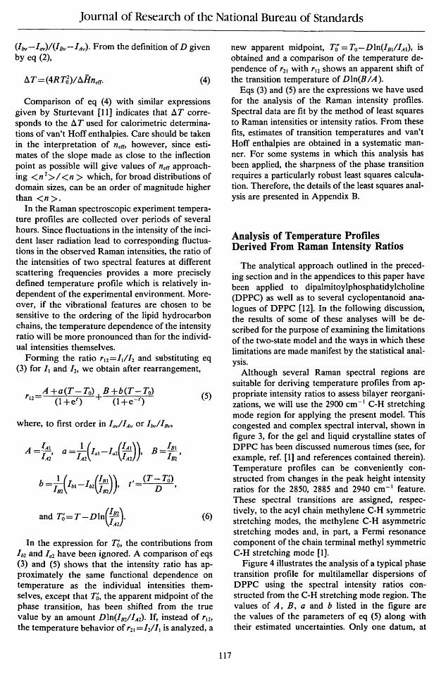
Although several Raman spectral regions are suitable for deriving temperature profiles from ap­propriate intensity ratios to assess bilayer reorgani­zations, we will use the 2900 cm- I C-H stretching mode region for applying the present model. This congested and complex spectral interval, shown in figure 3, for the gel and liquid crystalline states of DPPC has been discussed numerous times (see, for example, ref. [1] and references contained therein). Temperature profiles can be conveniently con­structed from changes in the peak height intensity ratios for the 2850, 2885 and 2940 cm -I feature. These spectral transitions are assigned, respec­tively, to the acyl chain methylene C-H symmetric stretching modes, the methylene C-H asymmetric stretching modes and, in part, a Fermi resonance component of the chain terminal methyl symmetric C-H stretching mode [1].

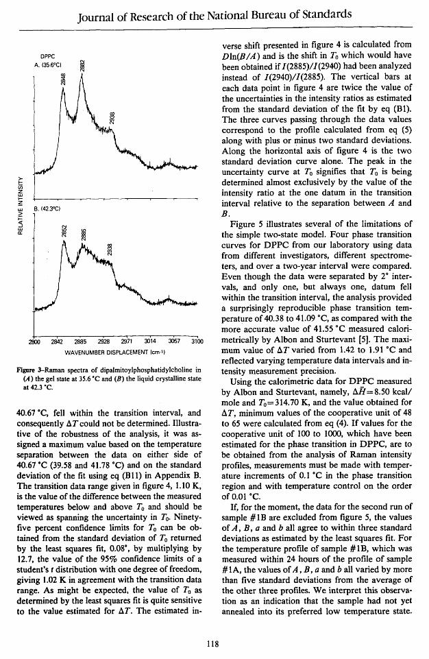
Figure 4 illustrates the analysis of a typical phase transition profile for multilamellar dispersions of DPPC using the spectral intensity ratios con­structed from the C-H stretching mode region. The values of A, B, a and b listed in the figure are the values of the parameters of eq (5) along with their estimated uncertainties. Only one datum, at

Journal of Research of the National Bureau of Standards

>­~ U) z w ~

~ w >

~ w a:

DPPC

A. (35.6°CI ~

B. (42.JOC)

2800 2842 2885 2928 2971 3014

WAVENUMBER DISPLACEMENT (cm-1)

3057 3100

Figure 3-Raman spectra of dipaImitoylphosphatidylcholine in (A) the gel state at 35.6 ·C and (B) the liquid crystal1ine state at 42.3 ·C.

40.67 °C, feU within the transition interval, and consequently aT could not be determined. Illustra­tive of the robustness of the analysis, it was as­signed a maximum value based on the temperature separation between the data on either side of 4O.67°C (39.58 and 41.78 °C) and on the standard deviation of the fit using eq (B 11) in Appendix B. The transition data range given in figure 4, 1.10 K, is the value of the difference between the measured temperatures below and above To and should be viewed as spanning the uncertainty in To. Ninety­five percent confidence limits for To can be ob­tained from the standard deviation of To returned by the least squares fit, 0.08°, by multiplying by 12.7, the value of the 95% confidence limits of a student's t distribution with one degree of freedom, giving 1.02 K in agreement with the transition data range. As might be expected, the value of To as determined by the least squares fit is quite sensitive to the value estimated for aT. The estimated in-

118

verse shift presented in figure 4 is calculated from Dln(B/A) and is the shift in To which would have been obtained if /(2885)//(2940) had been analyzed instead of /(2940)//(2885). The vertical bars at each data point in figure 4 are twice the value of the uncertainties in the intensity ratios as estimated from the standard deviation of the fit by eq (B 1). The three curves passing through the data values correspond to the profile calculated from eq (5) along with plus or minus two standard deviations. Along the horizontal axis of figure 4 is the two standard deviation curve alone. The peak in the uncertainty curve at To signifies that To is being determined almost exclusively by the value of the intensity ratio at the one datum in the transition interval relative to the separation between A and B.

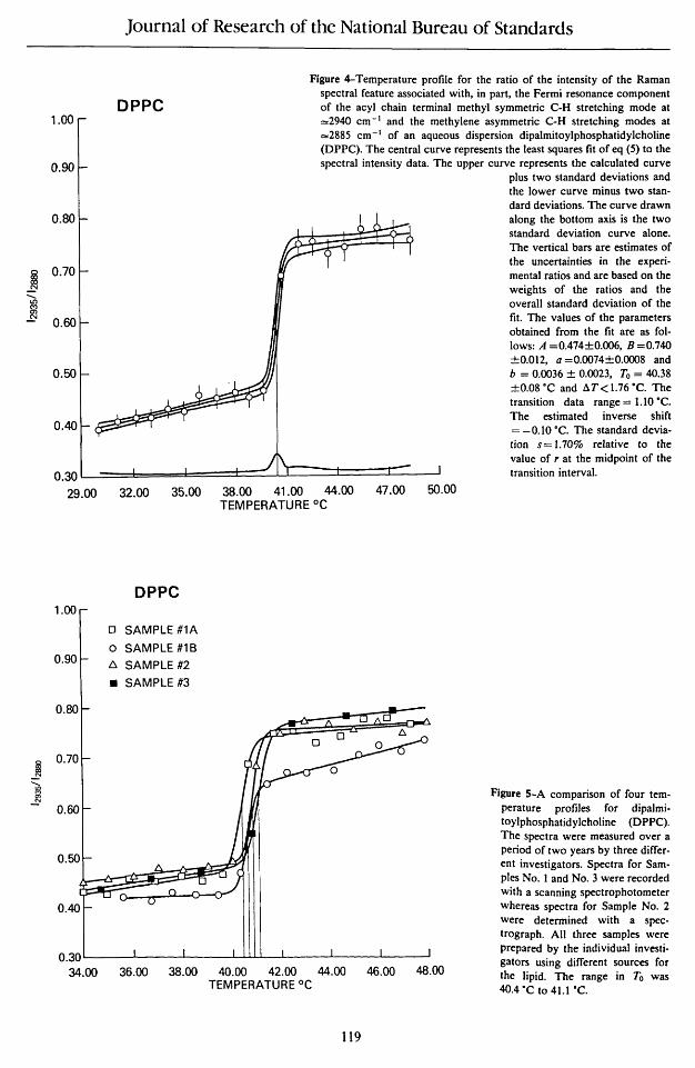
Figure 5 illustrates several of the limitations of the simple two-state model. Four phase transition curves for DPPC from our laboratory using data from different investigators, different spectrome­ters, and over a two-year interval were compared. Even though the data were separated by 2° inter­vals, and only one, but always one, datum feU within the transition interval, the analysis provided a surprisingly reproducible phase transition tem­perature of 40.38 to 41.09 °C, as compared with the more accurate value of 41.55 °C measured calori­metrically by Albon and Sturtevant [5]. The maxi­mum value of aT varied from 1.42 to 1.91 °C and reflected varying temperature data intervals and in­tensity measurement precision.

Using the calorimetric data for DPPC measured by Albon and Sturtevant, namely, Aii=8.50 kcall mole and To=314.70 K, and the value obtained for aT, minimum values of the cooperative unit of 48 to 65 were calculated from eq (4). If values for the cooperative unit of 100 to 1000, which have been estimated for the phase transition in DPPC, are to be obtained from the analysis of Raman intensity profiles, measurements must be made with temper­ature increments of 0.1 °C in the phase transition region and with temperature control on the order of 0.01 DC.

If, for the moment, the data for the second run of sample #IB are excluded from figure 5, the values of A, B, a and b all agree to within three standard deviations as estimated by the least squares fit. For the temperature profIle of sample #IB, which was measured within 24 hours of the profile of sample #IA, the values of A, B, a and b all varied by more than five standard deviations from the average of the other three profiles. We interpret this observa­tion as an indication that the sample had not yet annealed into its preferred low temperature state.

i ~ ........

It) M m ~

j .......

j

1.00

0.90

0.80

0.70

0.60

O.SO

0.40

0.30 29.00

1.00

0

0 0.90 6.

• 0.80

0.70

0.60

0.50

Journal of Research of the National Bureau of Standards

DPPC

Figure 4-Temperature profile for the ratio of the intensity of the Raman spectral feature associated with, in part, the Fermi resonance component of the acyl chain terminal methyl symmetric C-H stretching mode at =2940 cm -I and the methylene asymmetric C-H stretching modes at =2885 cm- I of an aqueous dispersion dipalmitoylphosphatidylcholine (DPPC). The central curve represents the least squares fit of eq (5) to the spectral intensity data. The upper curve represents the calculated curve

plus two standard deviations and the lower curve minus two stan­dard deviations. The curve drawn along the bottom axis is the two standard deviation curve alone. The vertical bars are estimates of the uncertainties in the experi­mental ratios and are based on the weights of the ratios and the overall standard deviation of the fit. The values of the parameters obtained from the fit are as fol­lows: A =0.474±0.006, B =0.740 ±0.012, a =0.0074±0.OOO8 and b = 0.0036 ± 0.0023, To = 40.38 ±0.08·C and dT < 1.76 ·C. The transition data range = UO ·C. The estimated inverse shift = -0.10 ·C. The standard devia­tion s = 1. 70% relative to the value of r at the midpoint of the transition interval.

32.00 35.00 38.00 41.00 44.00 TEMPERATURE °C

47.00 SO.OO

DPPC

SAMPLE #lA

SAMPLE #lB

SAMPLE #2

SAMPLE #3

0.30 L--__ ..L-__ ..L-__ ..L......L.J....L..I,._..L-__ "--__ "---_---'

Figure 5-A comparison of four tem­perature profiles for dipalmi­toylphosphatidyJcholine (DPPC). The spectra were measured over a period of two years by three differ­ent investigators. Spectra for Sam­ples No. 1 and No.3 were recorded with a scanning spectrophotometer whereas spectra for Sample No. 2 were determined with a spec­trograph. All three samples were prepared by the individual investi­gators using different sources for the lipid. The range in To was 4O.4·C to 4U ·C.

34.00 36.00 38.00 ~.OO 42.00 44.00 46.00 48.00 TEMPERATURE °C

119

Journal of Research of the National Bureau of Standards

Its bilayer structure appeared, on comparison with the values of the gel state intensity ratios for the other samples, to be as ordered at low tempera­tures, although it did not exhibit the gradual in­creasing disorder associated with the positive value of a. Its phase transition temperature, though somewhat higher than the others, did not change significantly nor did the transition interval to within measurement precision. The transition con­cluded at a much less disordered state than the other samples and then, corresponding to a large value of b, continued to disorder at a much greater rate than the others until reaching a comparable intensity ratio approximately 10 °c above the phase transition temperature. Although the two-state model cannot explain the molecular origins of such behavior, the fit of the data to eq (5) provides a basis of the intercomparison of temperature profiles in a methodical, reproducible, and quantitative manner.

The values of the asymptotic slopes observed for the temperature profiles of intensity ratios cannot be interpreted on the basis of domains of small size alone. Even for 'the three conforming profiles in figure 5, the values of the slopes at high and low temperature are on the order of 0.5% to 1.2%, somewhat greater than the value of 0.46% ob­tained for the broadest domain size distribution re-

1.60

1.40

1.20

-g ~ 1.00

.2 -­"C III Q

"C

~ 0.80 .::§

1,3/2-1P

o 2850/2885 o 2940/2850 t:. 2940/2885

O.60~--""""n-o.

0.40

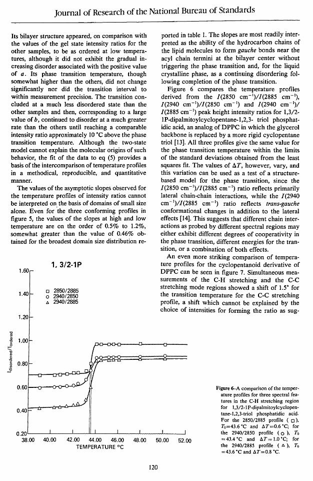
ported in table 1. The slopes are most readily inter­preted as the ability of the hydrocarbon chains of the lipid molecules to form gauche bonds near the acyl chain termini at the bilayer center without triggering the phase transition and, for the liquid crystalline phase, as a continuing disordering fol­lowing completion of the phase transition.

Figure 6 compares the temperature profiles derived from the 1(2850 cm- I)/1(2885 cm- I), 1(2940 cm-I)/1(2850 cm- I) and 1(2940 cm- I)! 1(2885 cm- I) peak height intensity ratios for 1,3/2-IP-dipalmitoylcyclopentane-l,2,3- triol phosphat­idic acid, an analog of DPPC in which the glycerol backbone is replaced by a more rigid cyclopentane trio I [13]. All three profiles give the same value for the phase transition temperature within the limits of the standard deviations obtained from the least squares fit. The values of 6.T, however, vary, and this variation can be used as a test of a structure­based model for the phase transition, since the 1(2850 cm- I)/1(2885 cm- I) ratio reflects primarily lateral chain-chain interactions, while the 1(2940 cm- I)/1(2885 cm- I) ratio reflects trans-gauche conformational changes in addition to the lateral effects [14]. This suggests that different chain inter­actions as probed by different spectral regions may either exhibit different degrees of cooperativity in the phase transition, different energies for the tran­sition, or a combination of both effects.

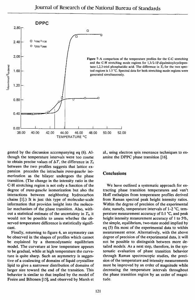
An even more striking comparison of tempera­ture profiles for the cyclopentanoid derivative of DPPC can be seen in figure 7. Simultaneous mea­surements of the C-H stretching and the C-C stretching mode regions showed a shift of 1.5° for the transition temperature for the C-C stretching profile, a shift which cannot be explained by the choice of intensities for forming the ratio as sug-

0.20 L--_---'-__ --'-_---IJ'-'-__ ....L.-__ ...L.-__ .L.-_----l

Figure 6-A comparison of the temper­ature profiles for three spectral fea­tures in the C-H stretching region for 1,3/2-1P-dipalmitoylcyc1open­tane-l,2,3-triol phosphatidic acid. For the 2850/2885 profile ( 0), To=43.6·C and t:..T=0.6 ·C; for the 2940/2850 profile (0), To = 43.4·C and t:..T = 1.0 ·C; for the 2940/2885 profile (t:..), To =43.6·C and t:..T=0.8 ·C.

38.00 40.00 42.00 M.OO ~.OO ~.OO 50.00 52.00 TEMPERATURE °C

120

Journal of Research of the National Bureau of Standards

DPPC 2.80

o

o

2.40 o 11090/11130

o 12935/12880

"0 ~ Ql

"0

..2 --

2.00

1.60

Figure 7-A comparison of the temperature profiles for the C-C stretching and the C-H stretching mode regions for 1,3/2-1P-dipalmitoylcyc1open­tane-l,2,3-triol phosphatidic acid. The difference in To for the two spec­tral regions is 1.5 ·C. Spectral data for both stretching mode regions were generated simultaneously.

"0 Ql

Ci:i "0 g 1.20 ~

0.80

0.40

O.OO~----~----~-L--~----~------~----~----~

38.00 40.00 42.00 M.OO 46.00 ~.OO 50.00 TEMPERATURE °C

52.00

gested by the discussion accompanying eq (6). Al­though the temperature intervals were too coarse to obtain precise values of ll.T, the difference in To between the two profiles suggests that lattice ex­pansion precedes the intrachain trans-gauche iso­merization as the bilayer undergoes the phase transition. (The change in the intensity ratio in the C-H stretching region is not only a function of the degree of trans-gauche isomerization but also the interactions between neighboring hydrocarbon chains [1].) It is just this type of molecular-scale information that provides insight into the molecu­lar mechanism of the phase transition. Also, with­out a statistical estimate of the uncertainty in To, it would not be possible to assess whether the ob­served temperature difference is statistically signifi­cant.

Finally, returning to figure 6, an asymmetry can be observed in the shapes of profiles which cannot be explained by a thermodynamic equilibrium model. The curvature at low temperature appears to be gradual, while at high temperature the curva­ture is quite sharp. Such an asymmetry is sugges­tive of a coalescing of domains of liquid crystalline lipid to give a narrower distribution of domains of larger size toward the end of the transition. This behavior is similar to that implied by the model of Freire and Biltonen [15], and observed by Marsh et

121

al., using electron spin resonance techniques to ex­amine the DPPC phase transition [16].

Conclusions

We have outlined a systematic approach for ex­tracting phase transition temperatures and van't Hoff enthalpies from temperature profiles derived from Raman spectral peak height intensity ratios. Within the degree of precision of the experimental data; namely, temperature intervals of I-2°C, tem­perature measurement accuracy of 0.1 °C, and peak height intensity measurement accuracy of 1 to 5%, the simple, equilibrium, two-state model implied by eq (5) fits most of the experimental data to within measurement error. Alternatively, with the above degree of precision of the experimental data, it will not be possible to distinguish between more de­tailed models. As a next step, therefore, in the sys­tematic evaluation of phase transition behavior through Raman spectroscopic studies, the preci­sion of the temperature and intensity measurements must be improved by an order of magnitude while decreasing the temperature intervals throughout the phase transition region by an order of magni­tude.

Journal of Research of the National Bureau of Standards

The advantage of deriving an analytical expres­sion for the Raman intensity behavior as a function of temperature lies in the development of statisti­cally based assessments of competing models. Data such as the exact profile curvature immediately preceding and following the phase transition and hysteresis effects can be used for model testing only when the data are reproducible and the mea­surement accuracy is controlled. A fruitful ap­proach is to combine improvements in the model with improvements in the experimental proce­dures, while using the statistical fit of analytical ex­pressions to the data as a basis for testing both the model and the adequacy of the data.

We appreciate the limitations of the present model. Although the two-state model conveys no information concerning the molecular nature or origin of the phase transition, the vibrational spec­troscopic data provide a means for directly moni­toring structural changes within the lipid bilayer over a large temperature range. The spectroscopic data are thus complementary to the calorimetric data. Moreover, the extraction of thermodynamic information from the spectroscopic studies pro­vides confirmation that the spectroscopic and calorimetric studies are responding to the same

APPENDIX A

Development of an Analytical Expression for Describing the Effect of Temperature on the Spectrum of a Molecular System in Terms of a Two-State Model.

The total Raman scattered intensity I at a partic­ular frequency v can be expressed as:

(At)

where IAv and Iav represent the scattering intensi­ties per molecule of molecules in each of two states A and B respectively and NA and NB are the num­ber of corresponding molecules per scattering vol­ume. The presence of other substances which may contribute to the overall scattering intensity will not affect the derivation that follows, since an ex­pression of the form

(A2)

122

phenomena. This aspect is particularly important in the study of lipid systems where sample history in­fluences the manifestation of conformational changes. As the next step in the development of the model, further detail concerning boundary effects between domains should be included along with a variation of the domain size distribution through the phase transition.

With an increased number of parameters in an analytic expression for the phase transition profiles comes a demand for greater data density through­out the phase transition region. We have already indicated the need for decreased temperature inter­vals. The comparison of temperature profiles ob­tained from different spectral regions promises to provide extremely useful tests for molecular-scale descriptions of the phase transition and the atten­dant molecular dynamics.

The course of the research described in this pa­per was strongly influenced by discussions with Dr. James S. Vincent and Dr. Terrell L. Hill. Their assistance is gratefully acknowledged.

where N' is the number of other scattering molecules, can be rewritten as

(A3)

I~v and IJn" as defined, are functions, therefore, of the composition of the sample as well as the intrin­sic scattering properties of the molecules of interest in states A and B. The temperature dependence of Iv, however, will be determined by the temperature dependence of NA and N B • The purpose of the fol­lowing mathematical treatment is to determine an explicit analytical expression for this temperature

Journal of Research of the National Bureau of Standards

dependence. And since the treatment deals only with the numbers NA and N B , it is also applicable to absorption spectra in concentration ranges where the transmitted intensity or its logarithm is a linear function of concentration; that is, where Beer's Law is obeyed.

We let Nn be the number of domains of size n of which N nA are in state A and NnB are in state B. The number of molecules in states A and B are then

(A4a)

and

(A4b)

In a closed, one-component system in contact with a heat bath at pressure constant pressure p, the differential expression for the internal energy of the system is

dE = TdS -pdV +l: p.ftndn +l: {LndNn (A5a) n n

where

p'n =(IINn)(oElon)s, V,N".m (A5b)

and

{Ln = (oEloNn)s. v, n.Nm (ASc)

and where m refers to· domains of all sizes other than n. The terms p.ftndn and {LndNn represent a separation of the total chemical potential of the sys­tem into two factors: one factor associated with changing the number of molecules in a given do­main and the other with changing the number of domains of a particular fixed size. In considering the effects of temperature on the number of do­mains in state A or state B, processes involving dn will be excluded. That is, only processes involving dNnA and dNnB , where dNnA = -dNnB , will be al­lowed.

The Gibbs free energy G for a system consisting of a mixture of domains of varying but distinguish­able size in one of two states, A or B, can then be written as:

(A6)

where

N=l: N n =l: NnA +NnB (A7) n n

is the total number of domains in the system and

123

where the chemical potentials {LnA and {LnB are the free energies of domains of size n in states A or B respectively. The condition for equilibrium be­tween states A and B is then:

(AS)

We define the partition coefficients for the system of domains as:

(A9)

where

r~i Z ~nI ni=(N;J! (AID)

and 'ni is the partition function for a domain of size n in the state i. The chemical potential can also be defined in terms of the Gibbs free energy as:

{Lni = (oG/aNni)r,p. n.Nmj (All)

and the Gibbs free energy can be expressed in terms of the partition function Z as:

G = -kTlnZ +pV. (AI2)

Combining equations (AS) through (A12) and in­voking Stirling's approximation for the logarithm of factorials gives:

where

AG~=-kTln~ 'nA

(A 13)

(AI4)

is the standard state free energy change for do­mains of size n. The number of molecules in state A is then given by:

(A15a)

and in state B by:

(A15b)

The temperature dependence of the intensity of a Raman spectral feature, which depends on NA and N B , is contained in the terms AG2IkT. As defined,

Journal of Research of the National Bureau of Standards

b.G~ is the difference in free energy between two domains of size n, one in state A and one in state B. For the simplest approximation to this difference, we let aG~ =n b.G~ and aG~B =n b.Gj where aG~ and b.Gj are the standard state free energies of indi­vidual molecules in states A and B respectively. This approximation is not exact because changes in the free energy of the domains will be affected by the domain boundaries. That is, we have defined the free energy of domains strictly for the internal degree of freedon associated with the order-disor­der phase transition of the lipid hydrocarbon chains. The free energy changes associated with this phase transition involve not only intramolecu­lar but intermolecular interactions as well. Individ­ual molecules at the boundaries between domains in different states will possess different intermolec­ular interaction energies in comparison with molecules within the domains themselves. The fac­torization of the partition function Z in eq (A9) into a product of single domain partition functions is also one that ignores boundary effects by assuming that the energy of interaction between domains is negligible. aG~ and aGj as defined represent an average value of the free energy per lipid molecule for an average domain size. The definition of what constitutes an individual molecular species is flex­ible. A molecular species could refer to a complete lipid molecule, a single hydrocarbon chain or even a single -CH2-CH2-CHr triad, the smallest unit for defining a trans or gauche conformation. The im­portant point is to ensure that the single unit free energy, b.G~ or aGj, is consistent with the defini­tion of that single molecular unit. In the remainder of this discussion, the unit will be taken as a single lipid molecule consisting of two chains.

Substitution of aG~A=nb.G~ and aG~B=naG8 into eq (A 15a) yields:

(AI6)

Note that a molar scale has been adopted for the exponential term so that aGo is the free energy change per mole of lipid molecules, R is the gas constant, but n retains its definition as the number of molecules per domain. If n is large and if aGo differs from 0, the exponential value is eq (A 16) rapidly approaches 0 or infinity depending on the sign of aGo and exhibits the discontinuity charac­teristic of a simple, first order phase transition. For smaller values of n (typically < tOO), the system exhibits a more continuous transition from state A to state B and can be described in a manner analogous to a two-component system in chemical

124

equilibrium. Since we know from experiment that pure lipid bilayers exhibit sharp phase transitions, we anticipate that n will be sufficiently large to allow expansion of aGo IT in a power series about T=To the temperature at which NA =NB :

aGOIT=(aGOIT)/ +a(aGolT)/aTI'T -To) T=To It=To

+ 1/2 a2(aGOIT)/aT2/ (T _TO)2. (A17) T=To

We define the standard state for each domain as the one for which NA =NB, so that b.Go=O at T=To. The derivative of aGolT with respect to T can be evaluated from the Gibbs-Helmholz equation ex­pressed in terms of differences in partial molar en­thalpies; namely,

(AI8)

where tJI =H B - HA • From this expression the sec­ond derivative of b.GoIT with respect to T can be calculated:

a2(b.Go/T)/a T2 =2WIT3 - (lIT2)(aW/a T)

(AI9)

Identifying ailla T as the molar specific heat at constant pressure, Cp , substituting eqs (AI8) and (AI9) into eq (AI7), and rearranging, the Taylor series expansion of AGO IT becomes:

b.GO IT = - (MITo)(T - To)ITo

+ (AiiITo-b.CpI2)[(T - To)lToF (A20)

In general, phase transitions for lipids have been observed to be quite sharp with complete conver­sion occurring over a range of less than· 10K. Thus, at phase transition temperatures on the order of 300 K, (T-To)lTo<.03 for T-To<10 K. l!.n­less b.Cp is an order of magnitude larger than WI To, the second term of eq (A20) can be ignored.

Wilkinson and Nagle have measured the heat ca­pacities of several lipids within 5 K above and be­low their main phase transitions [17]. As the phase transition temperature is approached from lower temperatures, Cp increases dramatically over the in­crease in Cp observed for normal alkanes [18]. Above TOt Cp is higher for the lipid systems than for the alkanes and decreases with increasing tem­perature. However, b.Cp does not appear to in­crease significantly and may actually be lower than the value determined for the solid-liquid phase

Journal of Research of the National Bureau of Standards

transitions in alkanes. The anomalously high values of Cp for lipids can be expected to occur when the phase transition is abnormally sharp; namely, over a temperature range of a degree or two where (T - To)/To<JXJ5. Consequently, we assume that the temperature dependence of flGo/T can be ade­quately described by the first term in eq (A20).

Substitution of the first term of eq (A20) into eq (A 16) gives for the number of molecules in state A ,

NA =l: nNn/(1 +etn) (A21) n

where, for simplicity, we have defined a reduced temperature ( as

(=(T - To)/D =MI(T - To)/RTJ (A22)

and the scale factor D as

(A23)

Similarly,

NB =l: nNn/(1 +e-tn) (A24)

n

!he magnitude of D may be estimated by letting illl=IO kcallmole and T 0=330 K so that D=20 K. For n = 100 and T - To> 1 K, NA <N /100.

Equations (A21) and (A24) are still too complex to be used for a least squares analysis of the temper­ature dependence of spectral intensities in the vicinity of a phase transition. The next step in the development is to replace the summations in eqs (A21) and (A24) with some suitable average over the distribution of domain sizes. The distribution of domain sizes is given by Nn as a function of n where Nn satisfies the following conditions: '

(A25)

and

(A26)

and where the moments of the distribution are de­fined as

<nk> =(1IiV) l: Nnn k (A27) n

The substitution of <n > into eq (A21),

125

would imply that <n >k= <nk> for an k, which would be inaccurate for all but the narrowest of distributions. A better approximation is

(A29)

Equations (A28) and (A29) both give the correct asymptotic behavior when compared with eq (A21). Both expressions have inflection points at (=0. However, eq (A29) also gives the correct slope at (=0, namely -N<n2>/4, whereas eq (A28) gives -N<N>2.

Since eq (A29) is congruent with eq (A21) at (=0 and ± 00 and since neither eq (A29) nor (A21) has any minima or maxima other than + 00 and - 00, we conclude that eq (A21) may be approxi­mated by a single term, namely

(A30)

where N=N<n> and neff=<n2>/<n >. Simi­larly, eq (A24) can be approximated by

(A31)

where N and neff have the same values as in eq (A30) in order to conserve the total number of molecules in the system. In practice, N and neff will be adjusted to give the best overall agreement be­tween eqs (A30,A31) and (A21,A24).

The accuracy of this single-term approximation can be tested by assuming a distribution function for n and comparing eq (A30) directly with eq (A21). This was done for a set of lognormal distri­butions as described in the main body of this paper.

Equations (A30) and (A31) can now be used in eq (AI) to describe the intensity of a Raman spec­tral feature as a function of temperature:

(A32)

where, as before, t =(T - To)/D, but where the ex­plicit reference to neff has been absorbed into the definition of D, namely,

D = (R TJ)/ MI neff (A33)

and where explicit reference to the number density N has been absorbed into the definitions of the scat­tering intensities IAI/ and 181.1'

Journal of Research of the National Bureau of Standards

APPENDIX B

The Least Squares Fit.

A computer program has been written to analyze the temperature dependence of Raman spectral data by fitting the data by the method of least squares to eq (5). Several features of this program are worth noting. Equation (5) is a linear function of the parameters A, B, a and b and a nonlinear function of To and D. Thus, the parameters of Eq (5) are evaluated using an iterative approach in which r is expanded in a Taylor series for each of the parameters about its currently estimated value. The series is terminated at its linear terms. The val­ues of robs - r calc are used as the dependent variables and the derivatives of r with respect to each of the parameters as the independent variables. From a linear fit of rom - r calc to the derivatives of r, the corrections to the parameters are obtained and the process is repeated using the new values of the parameters until the changes in the parameters for each iteration are significantly lower than the stan­dard deviations of the parameters.

The least squares fit is a weighted fit. If we as­sume that errors in the measured intensities are ran­dom, uncorrelated and are drawn from a single, normally distributed population of errors, and if we let s be the estimate of the standard deviation of that population, then the variance of a particular value of an intensity ratio is given by

(Bl)

where

rJ2=ltl1z and s2(IJ)=s2. Thus, the errors in the in­tensity ratios are not normally distributed but in­stead, depend on the magnitude of r and the intensity in the ratio denominator. Correspond­ingly, each ratio is given a weighting factor in the least squares fit proportional to the inverse square of its uncertainty, namely,

(B2)

By setting the proportionality factor to unity rather than lIs2 as suggested by eq (B1), the standard de-

126

viation returned by the fit should be a measure of the uncertainty of the Raman intensities. Compari­son of the standard deviation of the fit with esti­mates of the uncertainty in the measured intensities demonstrated that eq (5) is capable of fitting the experimental data to within currently obtained measurement error.

The algorithm for the least squares analysis fol­lows a Gram-Schmidt orthonormalization proce­dure. This procedure has been extensively tested [19] and a comparison between calculations using single and double precision gave identical results (to the degree of precision reported) indicating that the computation is free from numerical artifacts.

The major problem encountered in the analysis of the temperature profiles is associated with those situations in which the observed data are insuffi­cient to determine the apparent phase transition temperature To and the scaling parameter D. The remainder of this section will deal with those situa­tions.

The parameters To and D are determined solely from those data near T = To, whereas A , a, Band b are determined primarily by data from the high and low temperature asymptotes of eq (5). The range around To for which D and To can be determined is the range in which r deviates significantly from the asymptotes A +a(T-To) and B+b(T-To). A de­viation is defined as "significant" by the number of standard deviations by which a measured ratio dif­fers from each of the asymptotes. In particular, for a measured ratio to contribute to the determination of D and To, we require

(B3a)

and

I r; - (B +b (T; - To») I > Is/V w,. (B3b)

where rj is the value of the intensity ratio at the observed temperature Ti • A, a, B, b and To are the values of the parameters determined by the least squares fit; Wi is the weight of the i th datum used in the least squares fit; s is the standard deviation returned by the least squares fit; and! is a multi­plicative factor to allow for a more or less stringent test. The quantity, sNW;, is the estimated uncer­tainty in the experimental value of the r h ratio. Equations (B3a,b) state that for the purpose of con­tributing to the evaluation of To and D the value of an observed ratio must differ from both asymptotic limits by an amount greater than some mUltiple! of the expected measurement uncertainty at that tem-

Journal of Research of the National Bureau of Standards

perature. If the conditions of eqs (B3a,b) are met, we say that a measurement falls within the transi­tion interval. Equations (B3a,b) define the tempera­ture interval; the number of experimental data falling within this interval determines the reliability with which D and To can be estimated. In particu­lar, the number of data falling within this interval is the appropriate number to use in calculating the number of degrees of freedom for the estimation of confidence intervals from a student's t distribution.

If no measured temperature falls within the tran­sition interval, neither To nor D can be estimated by a least squares fit of the data to eq (5). If one mea­sured value falls within the interval, only To can be estimated, but not D. Furthermore, the value of the uncertainty in To returned by the least squares fit must be multiplied by a factor of 12.7, the value of t from the student's t distribution for one degree of freedom and confidence limits of 95%. If two mea­sured values fall within the interval, both To and D can be estimated, but the estimates of their uncer­tainties must be multiplied by 4.3, the value of t from the student's t distribution appropriate for two degrees of freedom. Should more than two measured values fall within the transition interval, To and D can be determined with increasing reli­ability.

When less than two points fall within the transi­tion interval, bounds can be placed on the values of To and D, even though To and D cannot be deter­mined precisely. In order to place bounds on To and D, bounds must be placed on the transition interval. The transition interval can be estimated by combining eqs (B3a,b) with eq (5) to give, ig­noring terms in a and b,

where

Fx =2In(IB-A I~W -1) (B4)

and W is the average weight of a measured value in the vicinity of the phase transition temperature. The transition interval Tx is the temperature inter­val over which r varies from A +a(T - To)±fs/ VW to B+b(T-To)+fsNW, where the upper sign is chosen if A <B and the lower sign if B <A.

If no measured temperature falls within the tran­sition interval, as tested by eqs (B3a,b), we know that

(B5)

where Td is the temperature interval between the

127

successive data pair above and below the phase transition temperature. Thus, from eq (B4)

(B6)

In calculating the value of A, a, Band b, D is held fixed at its average value in the range defined by eq (B6); namely

(B7)

and To is given as the midpoint between the two measured temperatures spanning the phase transi­tion interval. Depending on the precision of the Raman intensity measurements relative to the dif­ference between A and B, Fx typically varies from 2 to 9. Most of the time a value of/=2 is used in eqs (B3a,b) and (B4). Substitution of AT=4D into eq (B6) yields

(BSa)

and

(BSb)

If one measured temperature T; falls within the transition interval,

(B9)

where 2Td = T; + 1-T; -1 is twice the average data interval of the three measured temperatures spanning the transition interval. As with the case of no measured temperature falling within the inter­val, D is assigned the average value implied by the range of eq (B9); namely,

(BlO)

and AT is reported as

(BI1)

To is estimated by the least squares fit of all the data to eq (5) but is determined, almost exclusively, by the value of r at T; relative to A and B.

References

[lJ For a recent review, see Levin, I. W. In Adv. in Infrared and Raman Spectroscopy, 11, eds. R. J. H. Clark and R. E. Hester, pp. 1-48. New York: Wiley Heyden (1984).

[2J Steer, C. J.; J. S. Vincent and I. W. Levin, J. BioI. Chern. 2598052-5 (1984).

Journal of Research of the National Bureau of Standards

[3] Nagle, J. F., Ann. Rev. Phys. Chern. 31 157-195 (1980). [4] Israelachvili, J. N.; S. Marcelja and R. G. Horn, Quart.

Rev. Biophys. 13 121-200 (1980). [5] Albon, N., and J. M. Sturtevant, Proc. Natl. Acad. Sci.

U.S.A. 75 2258-6 (1978). [6] Hill, T. L., Thermodynamics of Small Systems, pp. 89-

133. New York: W. A. Benjamin, Inc. (1963). [7] Dluhy, R. A.; D. Moffatt, D. G. Cameron, R. Mendel­

sohn, and H. H. Mantsch, Can. J. Chern. 63 1925-32 (1985).

[8] Zimm, B. H., and J. K. Bragg, J. Chern. Phys. 31 526-35 (1959).

[9] Kendall, M. G., and A. Stuart, The Advanced Theory of Statistics, vol. I, pp. 168-73. New York: Hafner Publish­ing Co. (1969).

[10] Sturtevant, J. M., Proc. Natl. Acad. Sci. U.S.A. 79 3963-7 (1982).

[11]

[12]

[13]

[14]

[15]

[16]

[17)

[18]

[19]

Sturtevant, J. M., Ann. Rev. Biophys. Bioeng. 3 35-50 (1974). Kirchhoff, W. H.; A. J. Hancock and I. W. Levin, Bio­physical Journal 45:196a (1984). Singer, M. A.; M. K. Jain, H. Z. Sable, H. J. Pownall, W. W. Mantulin, M. D. Lister, and A. J. Hancock, Biochim. Biophys. Acta 731 373-7 (1983). Huang, C.; J. R. Lapides and I.W. Levin, J. Amer. Chern. Soc. 104 5926-30 (1982). Freire, E., and R. Biltonen, Biochim. Biophys. Acta 514 54-68 (1978). Marsh, D.; D. Watts and P. F. Knowles, Biochim. Bio­phys. Acta 465 500-14 (1977). Wilkinson, D. A., and J. F. Nagle, Biochim. Biophys. Acta 688 107-15 (1982). Finke, H. L.; M. E. Gross, G. Waddington, and H. M. Huffman, J. Am. Chern. Soc. 76 333-41 (1954). Wampler, R. H., J. Res. Natl. Bur. Stds. 73B 59-90 (1969).

128