Embed Size (px)
Citation preview
Descriptive Statistics:Numerical Measures
CONTENTS
STATISTICS IN PRACTICE: SMALL FRY DESIGN
3.1 MEASURES OF LOCATIONMeanMedianModePercentilesQuartiles
3.2 MEASURES OF VARIABILITYRangeInterquartile RangeVarianceStandard DeviationCoefficient of Variation
3.3 MEASURES OFDISTRIBUTION SHAPE,RELATIVE LOCATION, ANDDETECTION OF OUTLIERSDistribution Shapez-Scores
Chebyshev’s TheoremEmpirical RuleDetecting Outliers
3.4 EXPLORATORY DATAANALYSISFive-Number SummaryBox Plot
3.5 MEASURES OFASSOCIATION BETWEENTWO VARIABLESCovarianceInterpretation of the CovarianceCorrelation CoefficientInterpretation of the Correlation
Coefficient
3.6 THE WEIGHTED MEAN ANDWORKING WITH GROUPEDDATAWeighted MeanGrouped Data
CHAPTER 3
CH003.qxd 8/16/10 6:28 PM Page 86
Statistics in Practice 61
MAC PULL IN ART HERE, adjust size
as needed.
STATISTICS in PRACTICE
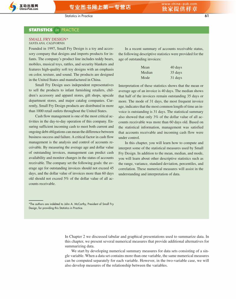
Founded in 1997, Small Fry Design is a toy and acces-sory company that designs and imports products for in-fants. The company’s product line includes teddy bears,mobiles, musical toys, rattles, and security blankets andfeatures high-quality soft toy designs with an emphasison color, texture, and sound. The products are designedin the United States and manufactured in China.
Small Fry Design uses independent representativesto sell the products to infant furnishing retailers, chil-dren’s accessory and apparel stores, gift shops, upscaledepartment stores, and major catalog companies. Cur-rently, Small Fry Design products are distributed in morethan 1000 retail outlets throughout the United States.
Cash flow management is one of the most critical ac-tivities in the day-to-day operation of this company. En-suring sufficient incoming cash to meet both current andongoing debt obligations can mean the difference betweenbusiness success and failure. A critical factor in cash flowmanagement is the analysis and control of accounts re-ceivable. By measuring the average age and dollar valueof outstanding invoices, management can predict cashavailability and monitor changes in the status of accountsreceivable. The company set the following goals: the av-erage age for outstanding invoices should not exceed 45days, and the dollar value of invoices more than 60 daysold should not exceed 5% of the dollar value of all ac-counts receivable.
In a recent summary of accounts receivable status,the following descriptive statistics were provided for theage of outstanding invoices:
Mean 40 daysMedian 35 daysMode 31 days
Interpretation of these statistics shows that the mean oraverage age of an invoice is 40 days. The median showsthat half of the invoices remain outstanding 35 days ormore. The mode of 31 days, the most frequent invoiceage, indicates that the most common length of time an in-voice is outstanding is 31 days. The statistical summaryalso showed that only 3% of the dollar value of all ac-counts receivable was more than 60 days old. Based onthe statistical information, management was satisfiedthat accounts receivable and incoming cash flow wereunder control.
In this chapter, you will learn how to compute andinterpret some of the statistical measures used by SmallFry Design. In addition to the mean, median, and mode,you will learn about other descriptive statistics such asthe range, variance, standard deviation, percentiles, andcorrelation. These numerical measures will assist in theunderstanding and interpretation of data.
SMALL FRY DESIGN*SANTA ANA, CALIFORNIA
STATISTICS in PRACTICE
*The authors are indebted to John A. McCarthy, President of Small FryDesign, for providing this Statistics in Practice.
In Chapter 2 we discussed tabular and graphical presentations used to summarize data. Inthis chapter, we present several numerical measures that provide additional alternatives forsummarizing data.
We start by developing numerical summary measures for data sets consisting of a sin-gle variable. When a data set contains more than one variable, the same numerical measurescan be computed separately for each variable. However, in the two-variable case, we willalso develop measures of the relationship between the variables.
CH003.qxd 8/16/10 6:28 PM Page 87
62 Chapter 3 Descriptive Statistics: Numerical Measures
SAMPLE MEAN
(3.1)x ��xi
n
In the three chapter appendixes we show how Minitab, Excel, and StatTools can be usedto compute the numerical measures described in the chapter.
In the preceding formula, the numerator is the sum of the values of the n observations. That is,
The Greek letter � is the summation sign.To illustrate the computation of a sample mean, let us consider the following class size
data for a sample of five college classes.
We use the notation x1, x2, x3, x4, x5 to represent the number of students in each of the five classes.
Hence, to compute the sample mean, we can write
The sample mean class size is 44 students.Another illustration of the computation of a sample mean is given in the following situ-
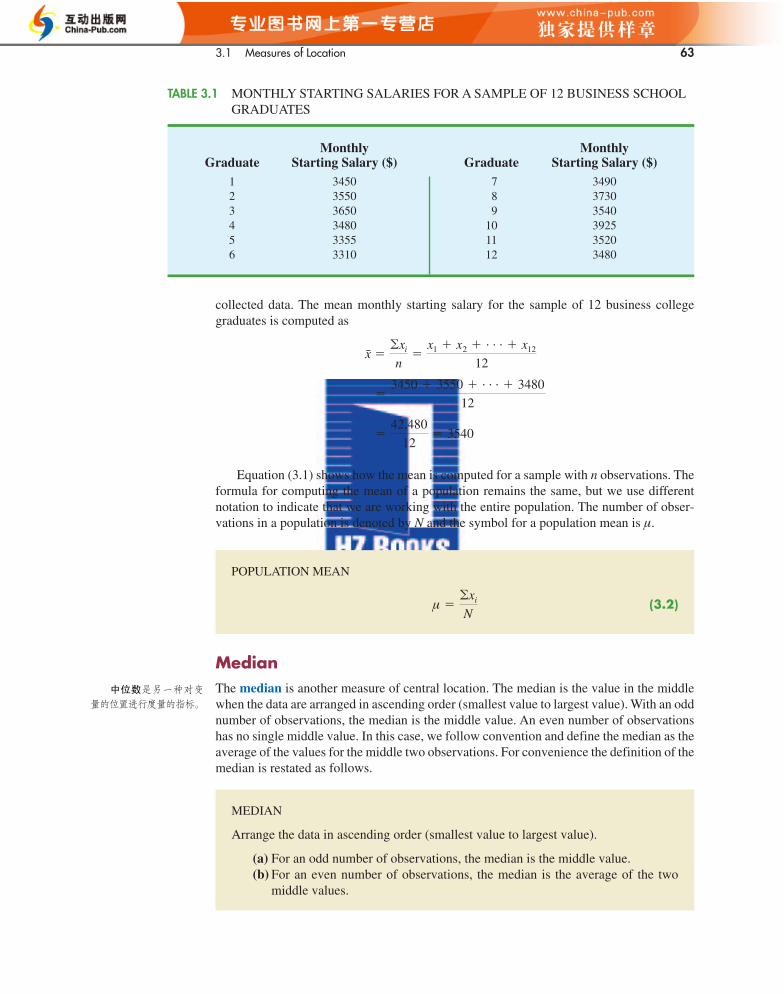
ation. Suppose that a college placement office sent a questionnaire to a sample of businessschool graduates requesting information on monthly starting salaries. Table 3.1 shows the
x ��xi
n�
x1 � x2 � x3 � x4 � x5
5�
46 � 54 � 42 � 46 � 32
5� 44
x1 � 46 x2 � 54 x3 � 42 x4 � 46 x5 � 32
46 54 42 46 32
�xi � x1 � x2 � . . . � xn
CH003.qxd 8/16/10 6:28 PM Page 88
平均数,或称平均值,
大概可以算得上是最常见
的对变量的位置进行度量
的一种方法。
Numerical measures of location, dispersion, shape, and association are introduced. Ifthe measures are computed for data from a sample, they are called sample statistics. If themeasures are computed for data from a population, they are called population parameters.In statistical inference, a sample statistic is referred to as the point estimator of the corre-sponding population parameter. In Chapter 7 we will discuss in more detail the process ofpoint estimation.
3.1 Measures of LocationMean
Perhaps the most important measure of location is the mean, or average value, for a vari-able. The mean provides a measure of central location for the data. If the data are for asample, the mean is denoted by ; if the data are for a population, the mean is denoted bythe Greek letter μ.
In statistical formulas, it is customary to denote the value of variable x for the first ob-servation by x1, the value of variable x for the second observation by x2, and so on. In gen-eral, the value of variable x for the ith observation is denoted by xi. For a sample with nobservations, the formula for the sample mean is as follows.
x
3.1 Measures of Location 63
CH003.qxd 8/16/10 6:28 PM Page 89
中位数是另一种对变
量的位置进行度量的指标。
POPULATION MEAN
(3.2)μ ��xi
N
collected data. The mean monthly starting salary for the sample of 12 business collegegraduates is computed as
Equation (3.1) shows how the mean is computed for a sample with n observations. Theformula for computing the mean of a population remains the same, but we use differentnotation to indicate that we are working with the entire population. The number of obser-vations in a population is denoted by N and the symbol for a population mean is μ.
�42,480
12� 3540
�3450 � 3550 � . . . � 3480
12
x ��xi
n�
x1 � x2 � . . . � x12
12
Median
The median is another measure of central location. The median is the value in the middlewhen the data are arranged in ascending order (smallest value to largest value). With an oddnumber of observations, the median is the middle value. An even number of observationshas no single middle value. In this case, we follow convention and define the median as theaverage of the values for the middle two observations. For convenience the definition of themedian is restated as follows.
Monthly MonthlyGraduate Starting Salary ($) Graduate Starting Salary ($)
1 3450 7 34902 3550 8 37303 3650 9 35404 3480 10 39255 3355 11 35206 3310 12 3480
TABLE 3.1 MONTHLY STARTING SALARIES FOR A SAMPLE OF 12 BUSINESS SCHOOLGRADUATES
MEDIAN
Arrange the data in ascending order (smallest value to largest value).
(a) For an odd number of observations, the median is the middle value.(b) For an even number of observations, the median is the average of the two
middle values.
64 Chapter 3 Descriptive Statistics: Numerical Measures
Let us apply this definition to compute the median class size for the sample of five collegeclasses. Arranging the data in ascending order provides the following list:
Because n � 5 is odd, the median is the middle value. Thus the median class size is 46 stu-dents. Even though this data set contains two observations with values of 46, each obser-vation is treated separately when we arrange the data in ascending order.
Suppose we also compute the median starting salary for the 12 business college gradu-ates in Table 3.1. We first arrange the data in ascending order:
3310 3355 3450 3480 3480 3490 3520 3540 3550 3650 3730 392514243
Middle Two Values
Because n � 12 is even, we identify the middle two values: 3490 and 3520. The median isthe average of these values.
Although the mean is the more commonly used measure of central location, in somesituations the median is preferred. The mean is influenced by extremely small and large datavalues. For instance, suppose that one of the graduates (see Table 3.1) had a starting salaryof $10,000 per month (maybe the individual’s family owns the company). If we change thehighest monthly starting salary in Table 3.1 from $3925 to $10,000 and recompute themean, the sample mean changes from $3540 to $4046. The median of $3505, however, isunchanged, because $3490 and $3520 are still the middle two values. With the extremelyhigh starting salary included, the median provides a better measure of central location thanthe mean. We can generalize to say that whenever a data set contains extreme values, themedian is often the preferred measure of central location.
Mode
Median �3490 � 3520
2� 3505
32 42 46 46 54
To illustrate the identification of the mode, consider the sample of five class sizes. Theonly value that occurs more than once is 46. Because this value, occurring with a fre-quency of 2, has the greatest frequency, it is the mode. As another illustration, consider thesample of starting salaries for the business school graduates. The only monthly startingsalary that occurs more than once is $3480. Because this value has the greatest frequency, itis the mode.
Situations can arise for which the greatest frequency occurs at two or more differentvalues. In these instances more than one mode exists. If the data contain exactly two modes,we say that the data are bimodal. If data contain more than two modes, we say that the dataare multimodal. In multimodal cases the mode is almost never reported because listing threeor more modes would not be particularly helpful in describing a location for the data.
MODE
The mode is the value that occurs with greatest frequency.
CH003.qxd 8/16/10 6:28 PM Page 90
第三种位置度量指标
是众数。 众数:出现频率最高
的数。
A third measure of location is the mode. The mode is defined as follows.
3.1 Measures of Location 65
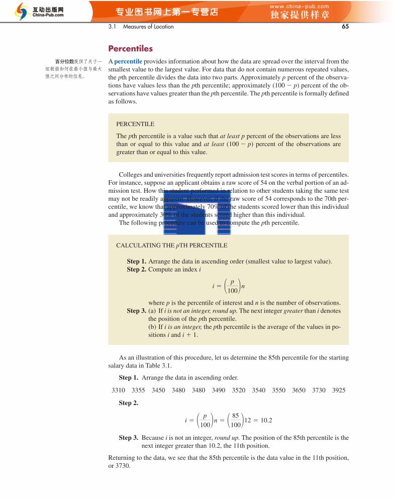
Percentiles
A percentile provides information about how the data are spread over the interval from thesmallest value to the largest value. For data that do not contain numerous repeated values,the pth percentile divides the data into two parts. Approximately p percent of the observa-tions have values less than the pth percentile; approximately (100 � p) percent of the ob-servations have values greater than the pth percentile. The pth percentile is formally definedas follows.
Colleges and universities frequently report admission test scores in terms of percentiles.For instance, suppose an applicant obtains a raw score of 54 on the verbal portion of an ad-mission test. How this student performed in relation to other students taking the same testmay not be readily apparent. However, if the raw score of 54 corresponds to the 70th per-centile, we know that approximately 70% of the students scored lower than this individualand approximately 30% of the students scored higher than this individual.
The following procedure can be used to compute the pth percentile.
PERCENTILE
The pth percentile is a value such that at least p percent of the observations are lessthan or equal to this value and at least (100 � p) percent of the observations aregreater than or equal to this value.
CALCULATING THE pTH PERCENTILE
Step 1. Arrange the data in ascending order (smallest value to largest value).Step 2. Compute an index i
where p is the percentile of interest and n is the number of observations.Step 3. (a) If i is not an integer, round up. The next integer greater than i denotes
the position of the pth percentile.(b) If i is an integer, the pth percentile is the average of the values in po-sitions i and i � 1.
As an illustration of this procedure, let us determine the 85th percentile for the startingsalary data in Table 3.1.
Step 1. Arrange the data in ascending order.
Step 2.
Step 3. Because i is not an integer, round up. The position of the 85th percentile is thenext integer greater than 10.2, the 11th position.
Returning to the data, we see that the 85th percentile is the data value in the 11th position,or 3730.
3310 3355 3450 3480 3480 3490 3520 3540 3550 3650 3730 3925
CH003.qxd 8/16/10 6:28 PM Page 91
百分位数提供了关于一
组数据如何在最小值与最大
值之间分布的信息。
i � � p
100�n
i � � p
100�n � � 85
100�12 � 10.2
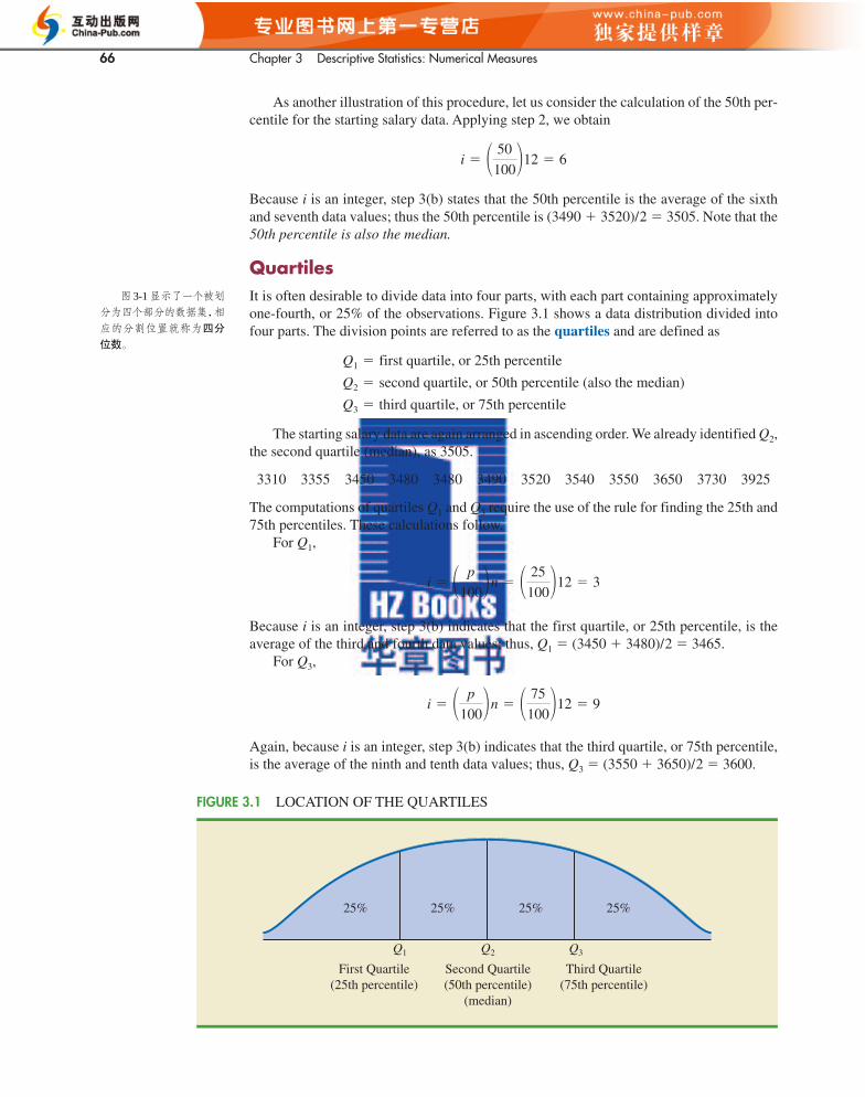
66 Chapter 3 Descriptive Statistics: Numerical Measures
Q1 Q2 Q3
25% 25%25%25%
First Quartile(25th percentile)
Second Quartile(50th percentile)
(median)
Third Quartile(75th percentile)
FIGURE 3.1 LOCATION OF THE QUARTILES
As another illustration of this procedure, let us consider the calculation of the 50th per-centile for the starting salary data. Applying step 2, we obtain
Because i is an integer, step 3(b) states that the 50th percentile is the average of the sixthand seventh data values; thus the 50th percentile is (3490 � 3520)/2 � 3505. Note that the50th percentile is also the median.
The starting salary data are again arranged in ascending order. We already identified Q2,the second quartile (median), as 3505.
The computations of quartiles Q1 and Q3 require the use of the rule for finding the 25th and75th percentiles. These calculations follow.
For Q1,
Again, because i is an integer, step 3(b) indicates that the third quartile, or 75th percentile,is the average of the ninth and tenth data values; thus, Q3 � (3550 � 3650)/2 � 3600.
3310 3355 3450 3480 3480 3490 3520 3540 3550 3650 3730 3925
Q3 � third quartile, or 75th percentile
Q2 � second quartile, or 50th percentile (also the median)
Q1 � first quartile, or 25th percentile
i � � 50
100�12 � 6
CH003.qxd 8/16/10 6:28 PM Page 92
图 3-1 显示了一个被划
分为四个部分的数据集,相
应的分割位置就称为四分
位数。
Quartiles
It is often desirable to divide data into four parts, with each part containing approximatelyone-fourth, or 25% of the observations. Figure 3.1 shows a data distribution divided intofour parts. The division points are referred to as the quartiles and are defined as
Because i is an integer, step 3(b) indicates that the first quartile, or 25th percentile, is theaverage of the third and fourth data values; thus, Q1 � (3450 � 3480)/2 � 3465.
For Q3,
i � � p
100�n � � 75
100�12 � 9
i � � p
100�n � � 25
100�12 � 3
3.1 Measures of Location 67
The quartiles divide the starting salary data into four parts, with each part containing25% of the observations.
3310 3355 3450 3480 3480 3490 3520 3540 3550 3650 3730 3925
We defined the quartiles as the 25th, 50th, and 75th percentiles. Thus, we computed thequartiles in the same way as percentiles. However, other conventions are sometimes usedto compute quartiles, and the actual values reported for quartiles may vary slightly de-pending on the convention used. Nevertheless, the objective of all procedures for comput-ing quartiles is to divide the data into four equal parts.
(Median)Q3 � 3600Q2 � 3505Q1 � 3465
���
moving the smallest 5% and the largest 5% of thedata values and then computing the mean of theremaining values. Using the sample with n � 12starting salaries, 0.05(12) � 0.6. Rounding this valueto 1 indicates that the 5% trimmed mean wouldremove the 1 smallest data value and the 1 largestdata value. The 5% trimmed mean using the 10 re-maining observations is 3524.50.
NOTES AND COMMENTS
It is better to use the median than the mean as ameasure of central location when a data set con-tains extreme values. Another measure, sometimesused when extreme values are present, is the trimmedmean. It is obtained by deleting a percentage of thesmallest and largest values from a data set and thencomputing the mean of the remaining values. Forexample, the 5% trimmed mean is obtained by re-
Exercises
Methods
1. Consider a sample with data values of 10, 20, 12, 17, and 16. Compute the mean and median.
2. Consider a sample with data values of 10, 20, 21, 17, 16, and 12. Compute the mean andmedian.
3. Consider a sample with data values of 27, 25, 20, 15, 30, 34, 28, and 25. Compute the 20th,25th, 65th, and 75th percentiles.
4. Consider a sample with data values of 53, 55, 70, 58, 64, 57, 53, 69, 57, 68, and 53. Com-pute the mean, median, and mode.
Applications
5. The Dow Jones Travel Index reported what business travelers pay for hotel rooms per nightin major U.S. cities (The Wall Street Journal, January 16, 2004). The average hotel roomrates for 20 cities are as follows:
Atlanta $163 Minneapolis $125Boston 177 New Orleans 167Chicago 166 New York 245Cleveland 126 Orlando 146Dallas 123 Phoenix 139Denver 120 Pittsburgh 134Detroit 144 San Francisco 167Houston 173 Seattle 162Los Angeles 160 St. Louis 145Miami 192 Washington, D.C. 207
CH003.qxd 8/16/10 6:28 PM Page 93
68 Chapter 3 Descriptive Statistics: Numerical Measures
a. What is the mean hotel room rate?b. What is the median hotel room rate?c. What is the mode?d. What is the first quartile?e. What is the third quartile?
6. During the 2007–2008 NCAAcollege basketball season, men’s basketball teams attemptedan all-time high number of 3-point shots, averaging 19.07 shots per game (AssociatedPress Sports, January 24, 2009). In an attempt to discourage so many 3-point shots and encourage more inside play, the NCAA rules committee moved the 3-point line back from19 feet, 9 inches to 20 feet, 9 inches at the beginning of the 2008–2009 basketball season.Shown in the following table are the 3-point shots taken and the 3-point shots made for asample of 19 NCAA basketball games during the 2008–2009 season.
3-Point Shots Shots Made 3-Point Shots Shots Made
23 4 17 720 6 19 1017 5 22 718 8 25 1113 4 15 616 4 10 58 5 11 3
19 8 25 828 5 23 721 7
a. What is the mean number of 3-point shots taken per game?b. What is the mean number of 3-point shots made per game?c. Using the closer 3-point line, players were making 35.2% of their shots. What per-
centage of shots were players making from the new 3-point line?d. What was the impact of the NCAA rules change that moved the 3-point line back to
20 feet, 9 inches for the 2008–2009 season? Would you agree with the AssociatedPress Sports article that stated, “Moving back the 3-point line hasn’t changed the gamedramatically”? Explain.
a. What is the mean endowment for these universities?b. What is the median endowment?c. What is the mode endowment?d. Compute the first and third quartiles.
University Endowment ($billion) University Endowment ($billion)
Columbia 7.2 Princeton 16.4Harvard 36.6 Stanford 17.2M.I.T. 10.1 Texas 16.1Michigan 7.6 Texas A&M 6.7Northwestern 7.2 Yale 22.9
CH003.qxd 8/16/10 6:28 PM Page 94
7. Endowment income is a critical part of the annual budgets at colleges and universities.A study by the National Association of College and University Business Officers re-ported that the 435 colleges and universities surveyed held a total of $413 billion in en-dowments. The 10 wealthiest universities are shown in the following table (The WallStreet Journal, January 27, 2009). Amounts are in billions of dollars.
3.2 Measures of Variability 69
e. What is the total endowment at these 10 universities? These universities represent2.3% of the 435 colleges and universities surveyed. What percentage of the total $413billion in endowments is held by these 10 universities?
f. The Wall Street Journal reported that over a recent five-month period, a downturn in the economy has caused endowments to decline 23%. What is the estimate of thedollar amount of the decline in the total endowments held by these 10 universities?Given this situation, what are some of the steps you would expect university admin-istrators to be considering?
CH003.qxd 8/16/10 6:28 PM Page 95
8. In automobile mileage and gasoline-consumption testing, 13 automobiles were road testedfor 300 miles in both city and highway driving conditions. The following data wererecorded for miles-per-gallon performance.
City: 16.2 16.7 15.9 14.4 13.2 15.3 16.8 16.0 16.1 15.3 15.2 15.3 16.2Highway: 19.4 20.6 18.3 18.6 19.2 17.4 17.2 18.6 19.0 21.1 19.4 18.5 18.7
Use the mean, median, and mode to make a statement about the difference in performancefor city and highway driving.
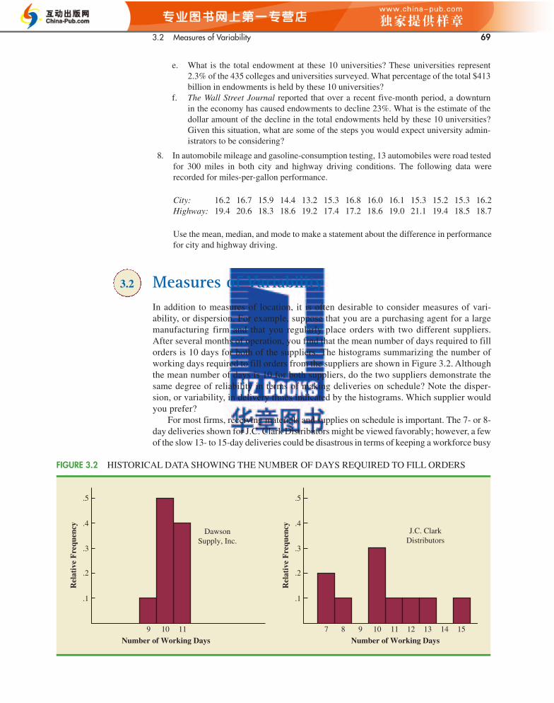
3.2 Measures of VariabilityIn addition to measures of location, it is often desirable to consider measures of vari-ability, or dispersion. For example, suppose that you are a purchasing agent for a largemanufacturing firm and that you regularly place orders with two different suppliers.After several months of operation, you find that the mean number of days required to fillorders is 10 days for both of the suppliers. The histograms summarizing the number ofworking days required to fill orders from the suppliers are shown in Figure 3.2. Althoughthe mean number of days is 10 for both suppliers, do the two suppliers demonstrate thesame degree of reliability in terms of making deliveries on schedule? Note the disper-sion, or variability, in delivery times indicated by the histograms. Which supplier wouldyou prefer?
For most firms, receiving materials and supplies on schedule is important. The 7- or 8-day deliveries shown for J.C. Clark Distributors might be viewed favorably; however, a fewof the slow 13- to 15-day deliveries could be disastrous in terms of keeping a workforce busy
Number of Working Days9 10 11
DawsonSupply, Inc.
Number of Working Days9 10 11 12
J.C. ClarkDistributors
13 14 157 8
.1
.2
.3
.4
Rel
ativ
e F
requ
ency
.5
.1
.2
.3
.4
Rel
ativ
e F
requ
ency
.5
FIGURE 3.2 HISTORICAL DATA SHOWING THE NUMBER OF DAYS REQUIRED TO FILL ORDERS
70 Chapter 3 Descriptive Statistics: Numerical Measures
CH003.qxd 8/16/10 6:28 PM Page 96
and production on schedule. This example illustrates a situation in which the variability inthe delivery times may be an overriding consideration in selecting a supplier. For most pur-chasing agents, the lower variability shown for Dawson Supply, Inc., would make Dawsonthe preferred supplier.
We turn now to a discussion of some commonly used measures of variability.
Range
The simplest measure of variability is the range.
RANGE
Range � Largest value � Smallest value
Let us refer to the data on starting salaries for business school graduates in Table 3.1. Thelargest starting salary is $3925 and the smallest is $3310. The range is 3925 � 3310 � 615.
Although the range is the easiest of the measures of variability to compute, it is seldomused as the only measure. The reason is that the range is based on only two of the observa-tions and thus is highly influenced by extreme values. Suppose one of the graduates received a starting salary of $10,000 per month. In this case, the range would be10,000 � 3310 � 6690 rather than 615. This large value for the range would not be espe-cially descriptive of the variability in the data because 11 of the 12 starting salaries areclosely grouped between 3310 and 3730.
Interquartile Range
极差是一种最简单的变
异指标。
一种克服了异常值的干
扰的变异指标是四分位距。
方差是利用所有数据进
行计算的一种变异指标。方
差取决于每个观察值与平均
值之间的差异。
A measure of variability that overcomes the dependency on extreme values is the inter-quartile range (IQR). This measure of variability is the difference between the third quar-tile, Q3, and the first quartile, Q1. In other words, the interquartile range is the range for themiddle 50% of the data.
For the data on monthly starting salaries, the quartiles are Q3 � 3600 and Q1 � 3465. Thus,the interquartile range is 3600 � 3465 � 135.
Variance
The variance is a measure of variability that utilizes all the data. The variance is based on thedifference between the value of each observation (xi) and the mean. The difference betweeneach xi and the mean ( for a sample, μ for a population) is called a deviation about the mean.For a sample, a deviation about the mean is written (xi � ); for a population, it is written(xi � μ). In the computation of the variance, the deviations about the mean are squared.
If the data are for a population, the average of the squared deviations is called the population variance. The population variance is denoted by the Greek symbol σ 2. For apopulation of N observations and with μ denoting the population mean, the definition of thepopulation variance is as follows.
xx
INTERQUARTILE RANGE
(3.3)IQR � Q3 � Q1
3.2 Measures of Variability 71
CH003.qxd 8/16/10 6:28 PM Page 97
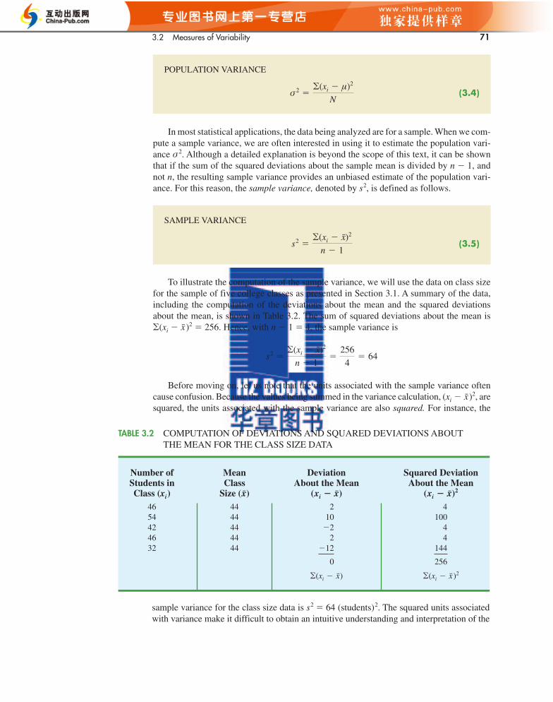
TABLE 3.2 COMPUTATION OF DEVIATIONS AND SQUARED DEVIATIONS ABOUTTHE MEAN FOR THE CLASS SIZE DATA
POPULATION VARIANCE
(3.4)σ 2 ��(xi � μ)2
N
SAMPLE VARIANCE
(3.5)s2 ��(xi � x)2
n � 1
In most statistical applications, the data being analyzed are for a sample. When we com-pute a sample variance, we are often interested in using it to estimate the population vari-ance σ 2. Although a detailed explanation is beyond the scope of this text, it can be shownthat if the sum of the squared deviations about the sample mean is divided by n � 1, andnot n, the resulting sample variance provides an unbiased estimate of the population vari-ance. For this reason, the sample variance, denoted by s2, is defined as follows.
To illustrate the computation of the sample variance, we will use the data on class sizefor the sample of five college classes as presented in Section 3.1. A summary of the data,including the computation of the deviations about the mean and the squared deviationsabout the mean, is shown in Table 3.2. The sum of squared deviations about the mean is�(xi � )2 � 256. Hence, with n � 1 � 4, the sample variance is
Before moving on, let us note that the units associated with the sample variance oftencause confusion. Because the values being summed in the variance calculation, (xi � )2, aresquared, the units associated with the sample variance are also squared. For instance, the
x
s2 ��(xi � x)2
n � 1�
256
4� 64
x
Number of Mean Deviation Squared DeviationStudents in Class About the Mean About the MeanClass (xi) Size ( ) ( ) ( )2
46 44 2 454 44 10 10042 44 �2 446 44 2 432 44 �12 144
0 256
�(xi � x)2�(xi � x)
xi � xxi � xx
sample variance for the class size data is s2 � 64 (students)2. The squared units associatedwith variance make it difficult to obtain an intuitive understanding and interpretation of the
72 Chapter 3 Descriptive Statistics: Numerical Measures
CH003.qxd 8/16/10 6:28 PM Page 98
numerical value of the variance. We recommend that you think of the variance as a measureuseful in comparing the amount of variability for two or more variables. In a comparison ofthe variables, the one with the largest variance shows the most variability. Further interpre-tation of the value of the variance may not be necessary.
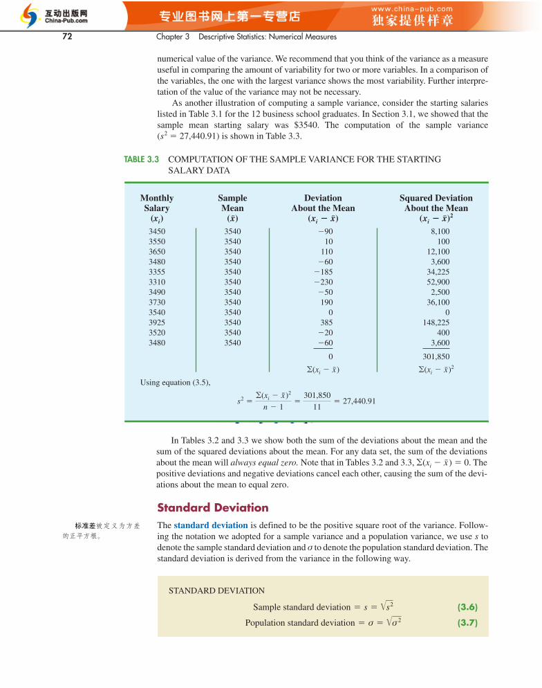
As another illustration of computing a sample variance, consider the starting salarieslisted in Table 3.1 for the 12 business school graduates. In Section 3.1, we showed that thesample mean starting salary was $3540. The computation of the sample variance(s2 � 27,440.91) is shown in Table 3.3.
TABLE 3.3 COMPUTATION OF THE SAMPLE VARIANCE FOR THE STARTING SALARY DATA
Standard Deviation
The standard deviation is defined to be the positive square root of the variance. Follow-ing the notation we adopted for a sample variance and a population variance, we use s todenote the sample standard deviation and σ to denote the population standard deviation. Thestandard deviation is derived from the variance in the following way.
标准差被定义为方差
的正平方根。
Monthly Sample Deviation Squared DeviationSalary Mean About the Mean About the Mean
(xi) ( ) ( ) ( )2
3450 3540 �90 8,1003550 3540 10 1003650 3540 110 12,1003480 3540 �60 3,6003355 3540 �185 34,2253310 3540 �230 52,9003490 3540 �50 2,5003730 3540 190 36,1003540 3540 0 03925 3540 385 148,2253520 3540 �20 4003480 3540 �60 3,600
0 301,850
Using equation (3.5),
s2 ��(xi � x)2
n � 1�
301,850
11� 27,440.91
�(xi � x)2�(xi � x)
xi � xxi � xx
STANDARD DEVIATION
(3.6)
(3.7)Population standard deviation � σ � �σ 2
Sample standard deviation � s � �s2
In Tables 3.2 and 3.3 we show both the sum of the deviations about the mean and thesum of the squared deviations about the mean. For any data set, the sum of the deviationsabout the mean will always equal zero. Note that in Tables 3.2 and 3.3, �(xi � ) � 0. Thepositive deviations and negative deviations cancel each other, causing the sum of the devi-ations about the mean to equal zero.
x
3.2 Measures of Variability 73
CH003.qxd 8/16/10 6:28 PM Page 99
For the class size data, we found a sample mean of 44 and a sample standard deviationof 8. The coefficient of variation is [(8/44) � 100]% � 18.2%. In words, the coefficient ofvariation tells us that the sample standard deviation is 18.2% of the value of the samplemean. For the starting salary data with a sample mean of 3540 and a sample standard devi-ation of 165.65, the coefficient of variation, [(165.65/3540) � 100]% � 4.7%, tells us thesample standard deviation is only 4.7% of the value of the sample mean. In general, the co-efficient of variation is a useful statistic for comparing the variability of variables that havedifferent standard deviations and different means.
在一些场合,我们可能
对一种衡量标准差与平均
数的相对大小的描述性统
计量产生兴趣。这种指标就
是变异系数,通常以百分数
形式表示。
Recall that the sample variance for the sample of class sizes in five college classes iss2 � 64. Thus, the sample standard deviation is For the data on startingsalaries, the sample standard deviation is
What is gained by converting the variance to its corresponding standard deviation? Re-call that the units associated with the variance are squared. For example, the sample vari-ance for the starting salary data of business school graduates is s2 � 27,440.91 (dollars)2.Because the standard deviation is the square root of the variance, the units of the variance,dollars squared, are converted to dollars in the standard deviation. Thus, the standard devia-tion of the starting salary data is $165.65. In other words, the standard deviation is mea-sured in the same units as the original data. For this reason the standard deviation is moreeasily compared to the mean and other statistics that are measured in the same units as theoriginal data.
Coefficient of Variation
In some situations we may be interested in a descriptive statistic that indicates how largethe standard deviation is relative to the mean. This measure is called the coefficient ofvariation and is usually expressed as a percentage.
s � �27,440.91 � 165.65.s � �64 � 8.
COEFFICIENT OF VARIATION
(3.8)�Standard deviation
Mean� 100�%
NOTES AND COMMENTS
1. Statistical software packages and spreadsheetscan be used to develop the descriptive statisticspresented in this chapter. After the data are entered into a worksheet, a few simple com-mands can be used to generate the desired out-put. In three chapter-ending appendixes weshow how Minitab, Excel, and StatTools can beused to develop descriptive statistics.
2. The standard deviation is a commonly usedmeasure of the risk associated with investing instock and stock funds (BusinessWeek, January 17,2000). It provides a measure of how monthly re-turns fluctuate around the long-run average return.
3. Rounding the value of the sample mean x andthe values of the squared deviations (xi � )2x
may introduce errors when a calculator is usedin the computation of the variance and standarddeviation. To reduce rounding errors, we rec-ommend carrying at least six significant digitsduring intermediate calculations. The result-ing variance or standard deviation can then berounded to fewer digits.
4. An alternative formula for the computation ofthe sample variance is
where � x2i � x2
1 � x22 � . . . � x2
n .
s2 �� x2
i � n x2
n � 1
74 Chapter 3 Descriptive Statistics: Numerical Measures
CH003.qxd 8/16/10 6:28 PM Page 100
a. Compute the mean price for models with a DVD player and the mean price for mod-els without a DVD player. What is the additional price paid to have a DVD playerincluded in a home theater unit?
b. Compute the range, variance, and standard deviation for the two samples. What doesthis information tell you about the prices for models with and without a DVD player?
Exercises
Methods
9. Consider a sample with data values of 10, 20, 12, 17, and 16. Compute the range and inter-quartile range.
10. Consider a sample with data values of 10, 20, 12, 17, and 16. Compute the variance andstandard deviation.
11. Consider a sample with data values of 27, 25, 20, 15, 30, 34, 28, and 25. Compute the range,interquartile range, variance, and standard deviation.
Applications
12. A bowler’s scores for six games were 182, 168, 184, 190, 170, and 174. Using these dataas a sample, compute the following descriptive statistics:a. Range c. Standard deviationb. Variance d. Coefficient of variation
13. A home theater in a box is the easiest and cheapest way to provide surround sound for ahome entertainment center. A sample of prices is shown here (Consumer Reports BuyingGuide, 2004). The prices are for models with a DVD player and for models without a DVD player.
14. Car rental rates per day for a sample of seven Eastern U.S. cities are as follows (The Wall StreetJournal, January 16, 2004).
a. Compute the mean, variance, and standard deviation for the car rental rates.b. A similar sample of seven Western U.S. cities showed a sample mean car rental
rate of $38 per day. The variance and standard deviation were 12.3 and 3.5, respec-tively. Discuss any difference between the car rental rates in Eastern and WesternU.S. cities.
Models with DVD Player Price Models without DVD Player Price
Sony HT-1800DP $450 Pioneer HTP-230 $300Pioneer HTD-330DV 300 Sony HT-DDW750 300Sony HT-C800DP 400 Kenwood HTB-306 360Panasonic SC-HT900 500 RCA RT-2600 290Panasonic SC-MTI 400 Kenwood HTB-206 300
City Daily Rate
Boston $43Atlanta 35Miami 34New York 58Orlando 30Pittsburgh 30Washington, D.C. 36
3.3 Measures of Distribution Shape, Relative Location, and Detection of Outliers 75
CH003.qxd 8/16/10 6:28 PM Page 101
15. The Los Angeles Times regularly reports the air quality index for various areas of South-ern California. A sample of air quality index values for Pomona provided the followingdata: 28, 42, 58, 48, 45, 55, 60, 49, and 50.a. Compute the range and interquartile range.b. Compute the sample variance and sample standard deviation.c. A sample of air quality index readings for Anaheim provided a sample mean of 48.5,
a sample variance of 136, and a sample standard deviation of 11.66. What compari-sons can you make between the air quality in Pomona and that in Anaheim on the basisof these descriptive statistics?
1The formula for the skewness of sample data:
Skewness �n
(n � 1)(n � 2) ��xi � x
s �3
16. Scores turned in by an amateur golfer at the Bonita Fairways Golf Course in BonitaSprings, Florida, during 2005 and 2006 are as follows:
2005 Season: 74 78 79 77 75 73 75 772006 Season: 71 70 75 77 85 80 71 79
a. Use the mean and standard deviation to evaluate the golfer’s performance over thetwo-year period.
b. What is the primary difference in performance between 2005 and 2006? What im-provement, if any, can be seen in the 2006 scores?
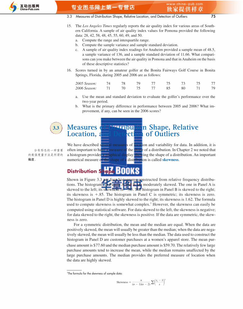
Shown in Figure 3.3 are four histograms constructed from relative frequency distribu-tions. The histograms in Panels A and B are moderately skewed. The one in Panel A isskewed to the left; its skewness is �.85. The histogram in Panel B is skewed to the right;its skewness is �.85. The histogram in Panel C is symmetric; its skewness is zero. The histogram in Panel D is highly skewed to the right; its skewness is 1.62. The formulaused to compute skewness is somewhat complex.1 However, the skewness can easily becomputed using statistical software. For data skewed to the left, the skewness is negative;for data skewed to the right, the skewness is positive. If the data are symmetric, the skew-ness is zero.
For a symmetric distribution, the mean and the median are equal. When the data arepositively skewed, the mean will usually be greater than the median; when the data are nega-tively skewed, the mean will usually be less than the median. The data used to construct thehistogram in Panel D are customer purchases at a women’s apparel store. The mean pur-
chase amount is $77.60 and the median purchase amount is $59.70. The relatively few largepurchase amounts tend to increase the mean, while the median remains unaffected by thelarge purchase amounts. The median provides the preferred measure of location whenthe data are highly skewed.
分布形态的一种重要
的数值度量方法是所谓的
偏度。
3.3 Measures of Distribution Shape, RelativeLocation, and Detection of OutliersWe have described several measures of location and variability for data. In addition, it isoften important to have a measure of the shape of a distribution. In Chapter 2 we noted thata histogram provides a graphical display showing the shape of a distribution. An importantnumerical measure of the shape of a distribution is called skewness.
Distribution Shape
76 Chapter 3 Descriptive Statistics: Numerical Measures
CH003.qxd 8/16/10 6:28 PM Page 102
0.3
0.25
0.2
0.15
0.1
0.05
0
0.35
0.3
0.25
0.2
0.15
0.1
0.05
0
0.35
0.3
0.25
0.2
0.15
0.1
0.05
0
Panel A: Moderately Skewed LeftSkewness � �.85
Panel C: SymmetricSkewness � 0
Panel B: Moderately Skewed RightSkewness � .85
Panel D: Highly Skewed RightSkewness � 1.62
0.4
0.35
0.3
0.25
0.2
0.15
0.1
0.05
0
FIGURE 3.3 HISTOGRAMS SHOWING THE SKEWNESS FOR FOUR DISTRIBUTIONS
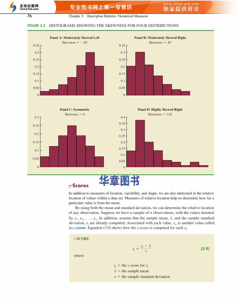
z-Scores
In addition to measures of location, variability, and shape, we are also interested in the relativelocation of values within a data set. Measures of relative location help us determine how far aparticular value is from the mean.
By using both the mean and standard deviation, we can determine the relative locationof any observation. Suppose we have a sample of n observations, with the values denotedby x1, x2, . . . , xn. In addition, assume that the sample mean, , and the sample standarddeviation, s, are already computed. Associated with each value, xi, is another value calledits z-score. Equation (3.9) shows how the z-score is computed for each xi.
x
z-SCORE
(3.9)
where
zi �
x �
s �
the z-score for xi
the sample mean
the sample standard deviation
zi �xi � x
s
3.3 Measures of Distribution Shape, Relative Location, and Detection of Outliers 77
The z-score is often called the standardized value. The z-score, zi, can be interpreted asthe number of standard deviations xi is from the mean . For example, z1 � 1.2 would indi-cate that x1 is 1.2 standard deviations greater than the sample mean. Similarly, z 2 � �.5would indicate that x 2 is .5, or 1/2, standard deviation less than the sample mean. A z-scoregreater than zero occurs for observations with a value greater than the mean, and a z-scoreless than zero occurs for observations with a value less than the mean. A z-score of zero in-dicates that the value of the observation is equal to the mean.
The z-score for any observation can be interpreted as a measure of the relative locationof the observation in a data set. Thus, observations in two different data sets with the samez-score can be said to have the same relative location in terms of being the same number ofstandard deviations from the mean.
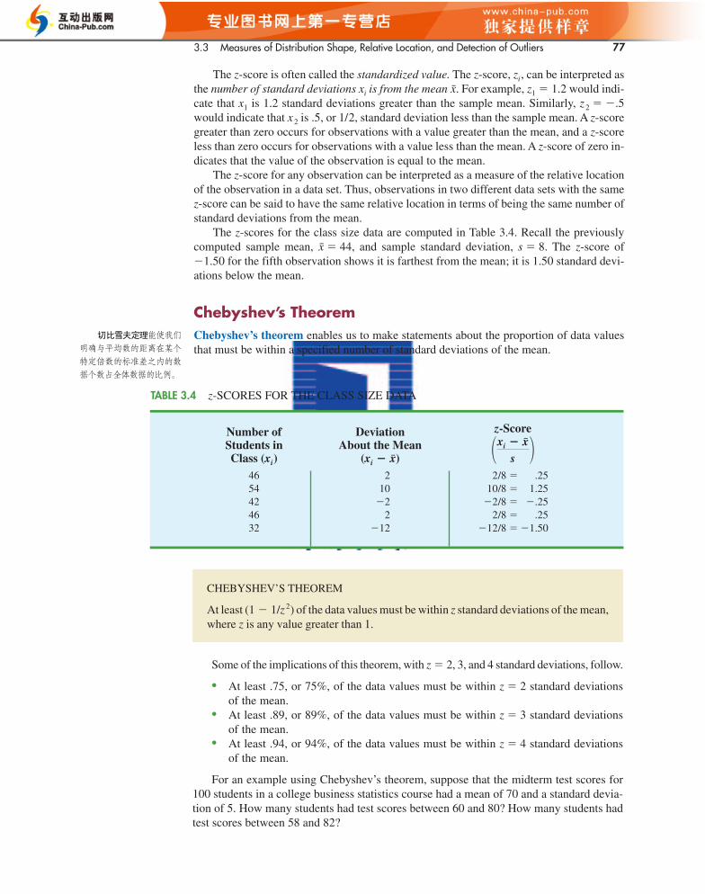
The z-scores for the class size data are computed in Table 3.4. Recall the previouslycomputed sample mean, � 44, and sample standard deviation, s � 8. The z-score of�1.50 for the fifth observation shows it is farthest from the mean; it is 1.50 standard devi-ations below the mean.
Chebyshev’s Theorem
Chebyshev’s theorem enables us to make statements about the proportion of data valuesthat must be within a specified number of standard deviations of the mean.
x
x
TABLE 3.4 z-SCORES FOR THE CLASS SIZE DATA
CH003.qxd 8/16/10 6:28 PM Page 105
CHEBYSHEV’S THEOREM
At least (1 � 1/z 2) of the data values must be within z standard deviations of the mean,where z is any value greater than 1.
Some of the implications of this theorem, with z � 2, 3, and 4 standard deviations, follow.
• At least .75, or 75%, of the data values must be within z � 2 standard deviationsof the mean.
• At least .89, or 89%, of the data values must be within z � 3 standard deviationsof the mean.
• At least .94, or 94%, of the data values must be within z � 4 standard deviationsof the mean.
For an example using Chebyshev’s theorem, suppose that the midterm test scores for100 students in a college business statistics course had a mean of 70 and a standard devia-tion of 5. How many students had test scores between 60 and 80? How many students hadtest scores between 58 and 82?
切比雪夫定理能使我们
明确与平均数的距离在某个
特定倍数的标准差之内的数
据个数占全体数据的比例。
Number of Deviation z-Score
46 2 2/8 � .2554 10 10/8 � 1.2542 �2 �2/8 � �.2546 2 2/8 � .2532 �12 �12/8 � �1.50
�xi � xs �About the Mean
(xi � x)Students inClass (xi)
78 Chapter 3 Descriptive Statistics: Numerical Measures
For the test scores between 60 and 80, we note that 60 is two standard deviations belowthe mean and 80 is two standard deviations above the mean. Using Chebyshev’s theorem,we see that at least .75, or at least 75%, of the observations must have values within twostandard deviations of the mean. Thus, at least 75% of the students must have scoredbetween 60 and 80.
For the test scores between 58 and 82, we see that (58 � 70)/5 � �2.4 indicates 58 is2.4 standard deviations below the mean and that (82 � 70)/5 � �2.4 indicates 82 is 2.4standard deviations above the mean. Applying Chebyshev’s theorem with z � 2.4, we have
At least 82.6% of the students must have test scores between 58 and 82.
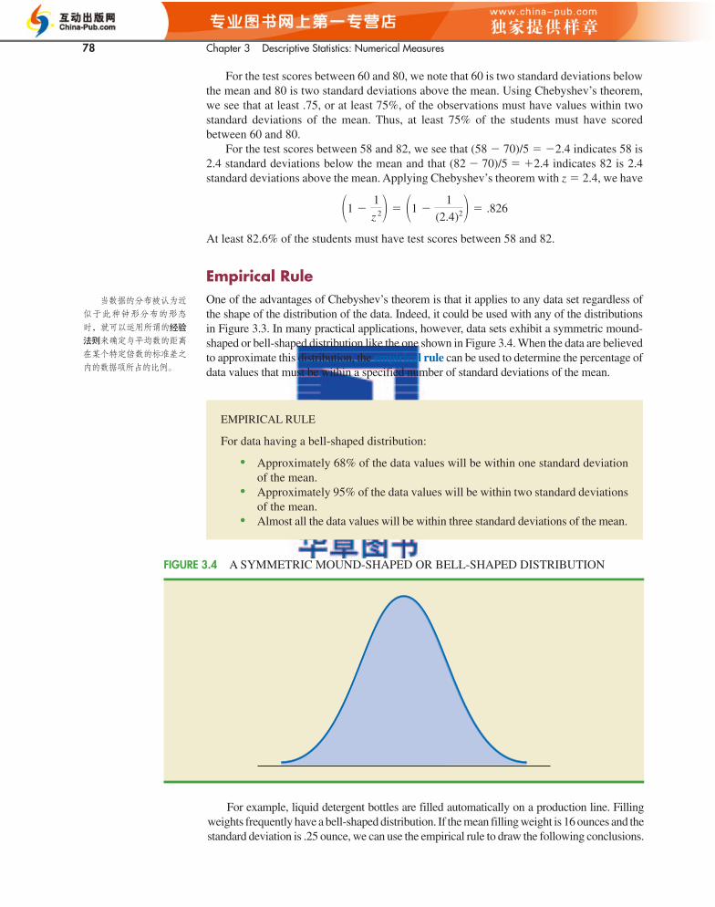
Empirical Rule
One of the advantages of Chebyshev’s theorem is that it applies to any data set regardless ofthe shape of the distribution of the data. Indeed, it could be used with any of the distributionsin Figure 3.3. In many practical applications, however, data sets exhibit a symmetric mound-shaped or bell-shaped distribution like the one shown in Figure 3.4. When the data are believedto approximate this distribution, the empirical rule can be used to determine the percentage ofdata values that must be within a specified number of standard deviations of the mean.
EMPIRICAL RULE
For data having a bell-shaped distribution:
• Approximately 68% of the data values will be within one standard deviationof the mean.
• Approximately 95% of the data values will be within two standard deviationsof the mean.
• Almost all the data values will be within three standard deviations of the mean.
CH003.qxd 8/16/10 6:28 PM Page 106
For example, liquid detergent bottles are filled automatically on a production line. Fillingweights frequently have a bell-shaped distribution. If the mean filling weight is 16 ounces and thestandard deviation is .25 ounce, we can use the empirical rule to draw the following conclusions.
FIGURE 3.4 A SYMMETRIC MOUND-SHAPED OR BELL-SHAPED DISTRIBUTION
当数据的分布被认为近
似于此种钟形分布的形态
时,就可以运用所谓的经验
法则来确定与平均数的距离
在某个特定倍数的标准差之
内的数据项所占的比例。
�1 �1
z 2� � �1 �1
(2.4)2� � .826
3.3 Measures of Distribution Shape, Relative Location, and Detection of Outliers 79
• Approximately 68% of the filled cartons will have weights between 15.75 and 16.25 ounces (within one standard deviation of the mean).
• Approximately 95% of the filled cartons will have weights between 15.50 and 16.50 ounces (within two standard deviations of the mean).
• Almost all filled cartons will have weights between 15.25 and 16.75 ounces (withinthree standard deviations of the mean).
Detection of Outliers
Sometimes a data set will have one or more observations with unusually large or unusuallysmall values. These extreme values are called outliers. Experienced statisticians take stepsto identify outliers and then review each one carefully. An outlier may be a data value thathas been incorrectly recorded. If so, it can be corrected before further analysis. An outliermay also be from an observation that was incorrectly included in the data set; if so, it canbe removed. Finally, an outlier may be an unusual data value that has been recorded cor-rectly and belongs in the data set. In such cases it should remain.
Standardized values (z-scores) can be used to identify outliers. Recall that the empiri-cal rule allows us to conclude that for data with a bell-shaped distribution, almost all thedata values will be within three standard deviations of the mean. Hence, in using z-scoresto identify outliers, we recommend treating any data value with a z-score less than �3 orgreater than �3 as an outlier. Such data values can then be reviewed for accuracy and todetermine whether they belong in the data set.
Refer to the z-scores for the class size data in Table 3.4. The z-score of �1.50 showsthat the fifth class size is farthest from the mean. However, this standardized value is wellwithin the �3 to �3 guideline for outliers. Thus, the z-scores do not indicate that outliersare present in the class size data.
NOTES AND COMMENTS
1. Chebyshev’s theorem is applicable for any dataset and can be used to state the minimum num-ber of data values that will be within a certainnumber of standard deviations of the mean. Ifthe data are known to be approximately bell-shaped, more can be said. For instance, the
CH003.qxd 8/16/10 6:28 PM Page 107
empirical rule allows us to say that approxi-mately 95% of the data values will be within twostandard deviations of the mean; Chebyshev’s
theorem allows us to conclude only that at least75% of the data values will be in that interval.
2. Before analyzing a data set, statisticians usuallymake a variety of checks to ensure the validityof data. In a large study it is not uncommon forerrors to be made in recording data values or inentering the values into a computer. Identifyingoutliers is one tool used to check the validity ofthe data.
Exercises
Methods
17. Consider a sample with data values of 10, 20, 12, 17, and 16. Compute the z-score for eachof the five observations.
18. Consider a sample with a mean of 500 and a standard deviation of 100. What are the z-scores for the following data values: 520, 650, 500, 450, and 280?
19. Consider a sample with a mean of 30 and a standard deviation of 5. Use Chebyshev’s the-orem to determine the percentage of the data within each of the following ranges:a. 20 to 40b. 15 to 45c. 22 to 38d. 18 to 42e. 12 to 48
有时一个数据集中可
能会包含一个或多个特别
大或特别小的观察值,像
这样的极端值我们称为异
常值。
80 Chapter 3 Descriptive Statistics: Numerical Measures
20. Suppose the data have a bell-shaped distribution with a mean of 30 and a standard devia-tion of 5. Use the empirical rule to determine the percentage of data within each of the fol-lowing ranges:a. 20 to 40b. 15 to 45c. 25 to 35
Applications
21. The results of a national survey showed that on average, adults sleep 6.9 hours per night.Suppose that the standard deviation is 1.2 hours.a. Use Chebyshev’s theorem to calculate the percentage of individuals who sleep be-
tween 4.5 and 9.3 hours.b. Use Chebyshev’s theorem to calculate the percentage of individuals who sleep be-
tween 3.9 and 9.9 hours.c. Assume that the number of hours of sleep follows a bell-shaped distribution. Use the
empirical rule to calculate the percentage of individuals who sleep between 4.5 and9.3 hours per day. How does this result compare to the value that you obtained usingChebyshev’s theorem in part (a)?
22. The national average for the math portion of the College Board’s SAT test is 515 (TheWorld Almanac, 2009). The College Board periodically rescales the test scores such thatthe standard deviation is approximately 100. Answer the following questions using a bell-shaped distribution and the empirical rule for the math test scores.
CH003.qxd 8/16/10 6:28 PM Page 108
a. What percentage of students have an SAT math score greater than 615?b. What percentage of students have an SAT math score greater than 715?c. What percentage of students have an SAT math score between 415 and 515?d. What percentage of students have an SAT math score between 315 and 615?
23. Florida Power & Light (FP&L) Company has enjoyed a reputation for quickly fixing itselectric system after storms. However, during the hurricane seasons of 2004 and 2005, anew reality was that the company’s historical approach to emergency electric systemrepairs was no longer good enough (The Wall Street Journal, January 16, 2006). Datashowing the days required to restore electric service after seven hurricanes during 2004and 2005 follow.
Hurricane Days to Restore Service
Charley 13Frances 12Jeanne 8Dennis 3Katrina 8Rita 2Wilma 18
Based on this sample of seven, compute the following descriptive statistics:a. Mean, median, and modeb. Range and standard deviationc. Should Wilma be considered an outlier in terms of the days required to restore elec-
tric service?d. The seven hurricanes resulted in 10 million service interruptions to customers. Do the
statistics show that FP&L should consider updating its approach to emergency elec-tric system repairs? Discuss.
24. A sample of 10 NCAA college basketball game scores provided the following data (USAToday, January 26, 2004).
81
WinningWinning Team Points Losing Team Points Margin
Arizona 90 Oregon 66 24Duke 85 Georgetown 66 19Florida State 75 Wake Forest 70 5Kansas 78 Colorado 57 21Kentucky 71 Notre Dame 63 8Louisville 65 Tennessee 62 3Oklahoma State 72 Texas 66 6
CH003.qxd 8/16/10 6:28 PM Page 109
a. Compute the mean and standard deviation for the points scored by the winning team.b. Assume that the points scored by the winning teams for all NCAA games follow a
bell-shaped distribution. Using the mean and standard deviation found in part (a),estimate the percentage of all NCAA games in which the winning team scores 84 ormore points. Estimate the percentage of NCAA games in which the winning teamscores more than 90 points.
c. Compute the mean and standard deviation for the winning margin. Do the data con-tain outliers? Explain.
Purdue 76 Michigan State 70 6Stanford 77 Southern Cal 67 10Wisconsin 76 Illinois 56 20
In Chapter 2 we introduced the stem-and-leaf display as a technique of exploratory dataanalysis. Recall that exploratory data analysis enables us to use simple arithmetic and easy-to-draw pictures to summarize data. In this section we continue exploratory data analysisby considering five-number summaries and box plots.
Five-Number Summary
In a five-number summary, the following five numbers are used to summarize the data:
1. Smallest value2. First quartile (Q1)3. Median (Q2)4. Third quartile (Q3)5. Largest value
The easiest way to develop a five-number summary is to first place the data in ascend-ing order. Then it is easy to identify the smallest value, the three quartiles, and the largestvalue. The monthly starting salaries shown in Table 3.1 for a sample of 12 business schoolgraduates are repeated here in ascending order.
3310 3355 3450 3480 3480 3490 3520 3540 3550 3650 3730 3925
(Median)Q3 � 3600Q2 � 3505Q1 � 3465
���
The median of 3505 and the quartiles Q1 � 3465 and Q3 � 3600 were computed in Sec-tion 3.1. Reviewing the data shows a smallest value of 3310 and a largest value of 3925.
在五数统计中,使用下
面五个数来对数据加以汇
总:(1) 最小值;(2)四分
之一分位数( 1);(3)中位
数( 2);(4)四分之三分位
数( 3);(5)最大值。
3.4 Exploratory Data Analysis
3.4 Exploratory Data Analysis
Q
82 Chapter 3 Descriptive Statistics: Numerical Measures
CH003.qxd 8/16/10 6:28 PM Page 110
Thus the five-number summary for the salary data is 3310, 3465, 3505, 3600, 3925. Ap-proximately one-fourth, or 25%, of the observations are between adjacent numbers in afive-number summary.
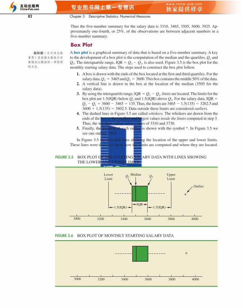
Box Plot
箱形图(又可译为箱
索图)是依据五数统计对
数据加以概括的一种图形
的方法。
A box plot is a graphical summary of data that is based on a five-number summary. A keyto the development of a box plot is the computation of the median and the quartiles, Q1 andQ3. The interquartile range, IQR � Q3 � Q1, is also used. Figure 3.5 is the box plot for themonthly starting salary data. The steps used to construct the box plot follow.
1. Abox is drawn with the ends of the box located at the first and third quartiles. For thesalary data, Q1 � 3465 and Q3 � 3600.This box contains the middle 50% of the data.
2. A vertical line is drawn in the box at the location of the median (3505 for the salary data).
3. By using the interquartile range, IQR � Q3 � Q1, limits are located. The limits for thebox plot are 1.5(IQR) below Q1 and 1.5(IQR) above Q3. For the salary data, IQR �Q3 � Q1 � 3600 � 3465 � 135. Thus, the limits are 3465 � 1.5(135) � 3262.5 and3600 � 1.5(135) � 3802.5. Data outside these limits are considered outliers.
4. The dashed lines in Figure 3.5 are called whiskers. The whiskers are drawn from theends of the box to the smallest and largest values inside the limits computed in step 3.Thus, the whiskers end at salary values of 3310 and 3730.
5. Finally, the location of each outlier is shown with the symbol *. In Figure 3.5 wesee one outlier, 3925.
In Figure 3.5 we included lines showing the location of the upper and lower limits.These lines were drawn to show how the limits are computed and where they are located.
IQR1.5(IQR) 1.5(IQR)
3200 34003000 3600 3800 4000
Q1 Q3Median Upper
LimitLowerLimit
*
Outlier
FIGURE 3.5 BOX PLOT OF THE STARTING SALARY DATA WITH LINES SHOWING THE LOWER AND UPPER LIMITS
*
3200 34003000 3600 3800 4000
FIGURE 3.6 BOX PLOT OF MONTHLY STARTING SALARY DATA
3.4 Exploratory Data Analysis 83
CH003.qxd 8/16/10 6:28 PM Page 111
Although the limits are always computed, generally they are not drawn on the box plots.Figure 3.6 shows the usual appearance of a box plot for the salary data.
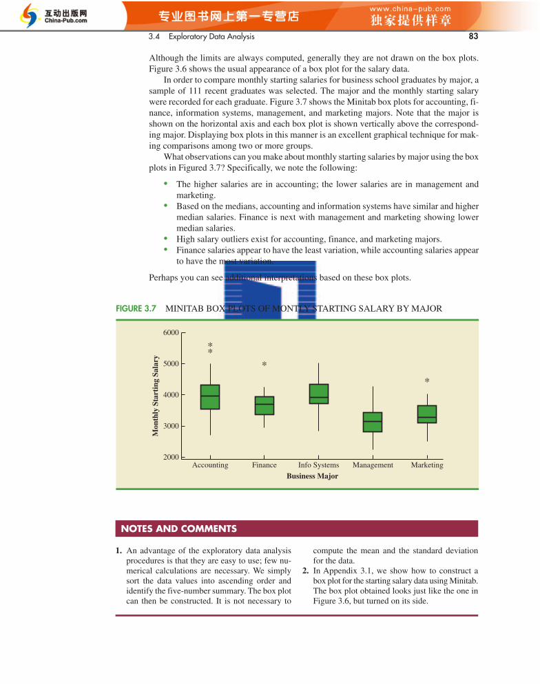
In order to compare monthly starting salaries for business school graduates by major, asample of 111 recent graduates was selected. The major and the monthly starting salarywere recorded for each graduate. Figure 3.7 shows the Minitab box plots for accounting, fi-nance, information systems, management, and marketing majors. Note that the major isshown on the horizontal axis and each box plot is shown vertically above the correspond-ing major. Displaying box plots in this manner is an excellent graphical technique for mak-ing comparisons among two or more groups.
What observations can you make about monthly starting salaries by major using the boxplots in Figured 3.7? Specifically, we note the following:
• The higher salaries are in accounting; the lower salaries are in management and marketing.
• Based on the medians, accounting and information systems have similar and highermedian salaries. Finance is next with management and marketing showing lowermedian salaries.
• High salary outliers exist for accounting, finance, and marketing majors.• Finance salaries appear to have the least variation, while accounting salaries appear
to have the most variation.
Perhaps you can see additional interpretations based on these box plots.
NOTES AND COMMENTS
1. An advantage of the exploratory data analysisprocedures is that they are easy to use; few nu-merical calculations are necessary. We simplysort the data values into ascending order andidentify the five-number summary. The box plotcan then be constructed. It is not necessary to
compute the mean and the standard deviationfor the data.
2. In Appendix 3.1, we show how to construct abox plot for the starting salary data using Minitab.The box plot obtained looks just like the one inFigure 3.6, but turned on its side.
2000
3000
4000
5000
6000
Accounting Finance Info Systems Management Marketing
Business Major
Mon
thly
Sta
rtin
g Sa
lary
FIGURE 3.7 MINITAB BOX PLOTS OF MONTLY STARTING SALARY BY MAJOR
84 Chapter 3 Descriptive Statistics: Numerical Measures
CH003.qxd 8/16/10 6:28 PM Page 112
Exercises
Methods
25. Consider a sample with data values of 27, 25, 20, 15, 30, 34, 28, and 25. Provide the five-number summary for the data.
26. Show the box plot for the data in exercise 36.
27. Show the five-number summary and the box plot for the following data: 5, 15, 18, 10, 8,12, 16, 10, 6.
28. A data set has a first quartile of 42 and a third quartile of 50. Compute the lower and upperlimits for the corresponding box plot. Should a data value of 65 be considered an outlier?
Applications
29. Some of the best-known food franchises and the number of retail locations for each areshown in the following table (The New York Times Almanac, 2010).
Franchise Locations Franchise Locations
Arby’s 2,558 McDonald’s 24,799Baskin-Robbins 5,889 Papa John’s 2,615Dairy Queen 5,619 Pizza Hut 10,238Domino’s 8,053 Quiznos 5,110Dunkin Donuts 8,082 Subway 29,612Hardee’s 1,397 Taco Bell 4,516KFC Corp 11,553
a. What is the largest franchise? How many retail locations does it have?b. What is the median number of locations for the franchises?c. Provide a five-number summary.d. Are there any outliers?e. Show the box plot.
30. A listing of 46 mutual funds and their 12-month total return percentage is shown in Table 3.5 (Smart Money, February 2004).a. What are the mean and median return percentages for these mutual funds?b. What are the first and third quartiles?c. Provide a five-number summary.d. Do the data contain any outliers? Show a box plot.

85
Return ReturnMutual Fund (%) Mutual Fund (%)
Alger Capital Appreciation 23.5 Nations Small Company 21.4Alger LargeCap Growth 22.8 Nations SmallCap Index 24.5Alger MidCap Growth 38.3 Nations Strategic Growth 10.4Alger SmallCap 41.3 Nations Value Inv 10.8AllianceBernstein Technology 40.6 One Group Diversified Equity 10.0Federated American Leaders 15.6 One Group Diversified Int’l 10.9Federated Capital Appreciation 12.4 One Group Diversified Mid Cap 15.1Federated Equity-Income 11.5 One Group Equity Income 6.6Federated Kaufmann 33.3 One Group Int’l Equity Index 13.2Federated Max-Cap Index 16.0 One Group Large Cap Growth 13.6Federated Stock 16.9 One Group Large Cap Value 12.8Janus Adviser Int’l Growth 10.3 One Group Mid Cap Growth 18.7Janus Adviser Worldwide 3.4 One Group Mid Cap Value 11.4Janus Enterprise 24.2 One Group Small Cap Growth 23.6Janus High-Yield 12.1 PBHG Growth 27.3Janus Mercury 20.6 Putnam Europe Equity 20.4Janus Overseas 11.9 Putnam Int’l Capital Opportunity 36.6Janus Worldwide 4.1 Putnam International Equity 21.5Nations Convertible Securities 13.6 Putnam Int’l New Opportunity 26.3Nations Int’l Equity 10.7 Strong Advisor Mid Cap Growth 23.7Nations LargeCap Enhd. Core 13.2 Strong Growth 20 11.7Nations LargeCap Index 13.5 Strong Growth Inv 23.2Nation MidCap Index 19.5 Strong Large Cap Growth 14.5
TABLE 3.5 TWELVE-MONTH RETURN FOR MUTUAL FUNDS
CH003.qxd 8/16/10 6:28 PM Page 115
3.5 Measures of Association Between Two VariablesThus far we have examined numerical methods used to summarize the data for one variableat a time. Often a manager or decision maker is interested in the relationship between twovariables. In this section we present covariance and correlation as descriptive measures ofthe relationship between two variables.
For a sample of size n with the observations (x1, y1), (x2, y2), and so on, the sample covari-ance is defined as follows:
SAMPLE COVARIANCE
(3.10)sxy ��(xi � x)(
yi � y)
n � 1
协方差一般用来描述
两个变量之间的线性关系。
Covariance
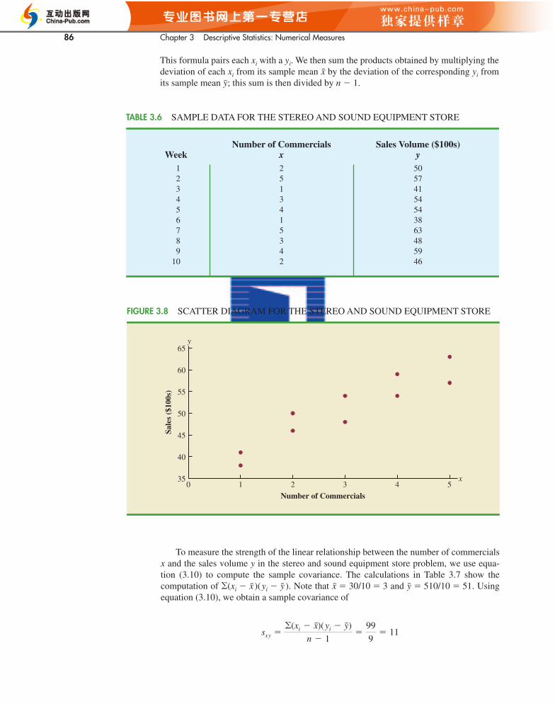
We begin by reconsidering the application concerning a stereo and sound equipmentstore in San Francisco as presented in Section 2.4. The store’s manager wants to determinethe relationship between the number of weekend television commercials shown and thesales at the store during the following week. Sample data with sales expressed in hundredsof dollars are provided in Table 3.6. It shows 10 observations (n � 10), one for each week.The scatter diagram in Figure 3.8 shows a positive relationship, with higher sales (y) asso-ciated with a greater number of commercials (x). In fact, the scatter diagram suggests thata straight line could be used as an approximation of the relationship. In the following dis-cussion, we introduce covariance as a descriptive measure of the linear association betweentwo variables.
3.5 Measures of Association Between Two Variables
86 Chapter 3 Descriptive Statistics: Numerical Measures
This formula pairs each xi with a yi. We then sum the products obtained by multiplying thedeviation of each xi from its sample mean by the deviation of the corresponding yi fromits sample mean ; this sum is then divided by n � 1.y
x
CH003.qxd 8/16/10 6:28 PM Page 116
To measure the strength of the linear relationship between the number of commercialsx and the sales volume y in the stereo and sound equipment store problem, we use equa-tion (3.10) to compute the sample covariance. The calculations in Table 3.7 show thecomputation of �(xi � )(yi � ). Note that � 30/10 � 3 and � 510/10 � 51. Usingequation (3.10), we obtain a sample covariance of
sxy ��(xi � x)(yi � y)
n � 1�
99
9� 11
yxyx
35
40
45
50
55
60
65
0 1 2 3 4 5
Number of Commercials
x
y
Sale
s ($
100s
)
FIGURE 3.8 SCATTER DIAGRAM FOR THE STEREO AND SOUND EQUIPMENT STORE
Number of Commercials Sales Volume ($100s)Week x y
1 2 502 5 573 1 414 3 545 4 546 1 387 5 638 3 489 4 59
10 2 46
TABLE 3.6 SAMPLE DATA FOR THE STEREO AND SOUND EQUIPMENT STORE
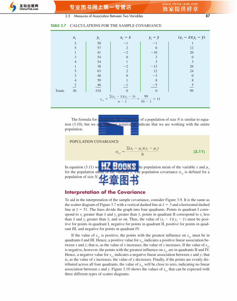
3.5 Measures of Association Between Two Variables 87
xi yi ( )( )
2 50 �1 �1 15 57 2 6 121 41 �2 �10 203 54 0 3 04 54 1 3 31 38 �2 �13 265 63 2 12 243 48 0 �3 04 59 1 8 82 46 �1 �5 5
Totals 30 510 0 0 99
sx y ��(xi � x)(
yi � y)
n � 1�
99
10 � 1� 11
yi � yxi � xyi � yxi � x
TABLE 3.7 CALCULATIONS FOR THE SAMPLE COVARIANCE
CH003.qxd 8/16/10 6:28 PM Page 117
In equation (3.11) we use the notation μx for the population mean of the variable x and μy
for the population mean of the variable y. The population covariance σxy is defined for apopulation of size N.
Interpretation of the Covariance
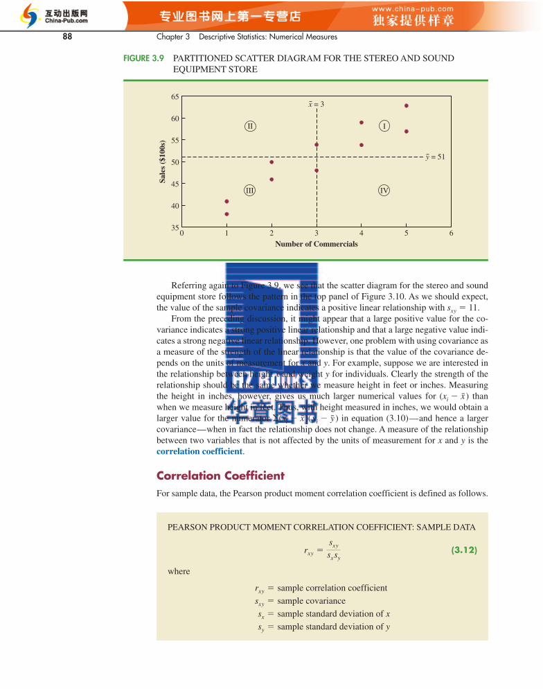
To aid in the interpretation of the sample covariance, consider Figure 3.9. It is the same asthe scatter diagram of Figure 3.7 with a vertical dashed line at � 3 and a horizontal dashedline at � 51. The lines divide the graph into four quadrants. Points in quadrant I corre-spond to xi greater than and yi greater than , points in quadrant II correspond to xi lessthan and yi greater than , and so on. Thus, the value of (xi � )(yi � ) must be posi-tive for points in quadrant I, negative for points in quadrant II, positive for points in quad-rant III, and negative for points in quadrant IV.
yxyxyx
yx
The formula for computing the covariance of a population of size N is similar to equa-tion (3.10), but we use different notation to indicate that we are working with the entirepopulation.
POPULATION COVARIANCE
(3.11)σx y ��(xi � μx)(
yi � μy)
N
If the value of sxy is positive, the points with the greatest influence on sxy must be inquadrants I and III. Hence, a positive value for sxy indicates a positive linear association be-tween x and y; that is, as the value of x increases, the value of y increases. If the value of sxy
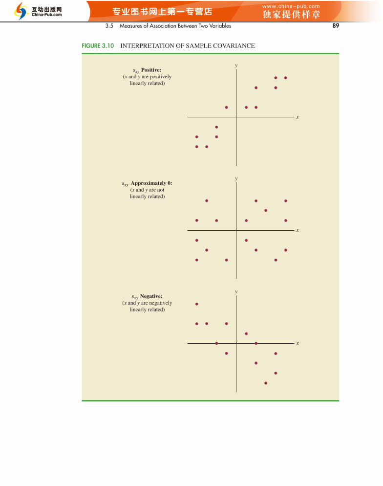
is negative, however, the points with the greatest influence on sxy are in quadrants II and IV.Hence, a negative value for sxy indicates a negative linear association between x and y; thatis, as the value of x increases, the value of y decreases. Finally, if the points are evenly dis-tributed across all four quadrants, the value of sxy will be close to zero, indicating no linearassociation between x and y. Figure 3.10 shows the values of sxy that can be expected withthree different types of scatter diagrams.
88 Chapter 3 Descriptive Statistics: Numerical Measures
65
60
55
50
45
40
35
Sale
s ($
100s
)
0 1 2 3
Number of Commercials4 5 6
II
III
I
IV
x = 3
y = 51
FIGURE 3.9 PARTITIONED SCATTER DIAGRAM FOR THE STEREO AND SOUNDEQUIPMENT STORE
CH003.qxd 8/16/10 6:28 PM Page 118
Correlation Coefficient
For sample data, the Pearson product moment correlation coefficient is defined as follows.
PEARSON PRODUCT MOMENT CORRELATION COEFFICIENT: SAMPLE DATA
(3.12)
where
rxy �
sxy �
sx �
sy �
sample correlation coefficient
sample covariance
sample standard deviation of x
sample standard deviation of y
rxy �sxy
sx sy
Referring again to Figure 3.9, we see that the scatter diagram for the stereo and soundequipment store follows the pattern in the top panel of Figure 3.10. As we should expect,the value of the sample covariance indicates a positive linear relationship with sxy � 11.
From the preceding discussion, it might appear that a large positive value for the co-variance indicates a strong positive linear relationship and that a large negative value indi-cates a strong negative linear relationship. However, one problem with using covariance asa measure of the strength of the linear relationship is that the value of the covariance de-pends on the units of measurement for x and y. For example, suppose we are interested inthe relationship between height x and weight y for individuals. Clearly the strength of therelationship should be the same whether we measure height in feet or inches. Measuringthe height in inches, however, gives us much larger numerical values for (xi � ) thanwhen we measure height in feet. Thus, with height measured in inches, we would obtain alarger value for the numerator �(xi � )(yi � ) in equation (3.10)—and hence a largercovariance—when in fact the relationship does not change. A measure of the relationshipbetween two variables that is not affected by the units of measurement for x and y is thecorrelation coefficient.
yx
x
3.5 Measures of Association Between Two Variables 89
y
x
sxy Positive:(x and y are positively
linearly related)
y
x
sxy Approximately 0:(x and y are notlinearly related)
y
x
sxy Negative:(x and y are negatively
linearly related)
FIGURE 3.10 INTERPRETATION OF SAMPLE COVARIANCE
CH003.qxd 8/16/10 6:28 PM Page 119
90 Chapter 3 Descriptive Statistics: Numerical Measures
Equation (3.12) shows that the Pearson product moment correlation coefficient forsample data (commonly referred to more simply as the sample correlation coefficient) iscomputed by dividing the sample covariance by the product of the sample standard devia-tion of x and the sample standard deviation of y.
Let us now compute the sample correlation coefficient for the stereo and sound equip-ment store. Using the data in Table 3.7, we can compute the sample standard deviations forthe two variables:
Now, because sxy � 11, the sample correlation coefficient equals
rxy �sxy
sxsy
�11
(1.49)(7.93)� .93
sy � � �(
yi � y)2
n � 1� �566
9� 7.93
sx � � �(xi � x)2
n � 1� �20
9� 1.49
CH003.qxd 8/16/10 6:28 PM Page 120
The formula for computing the correlation coefficient for a population, denoted by theGreek letter �xy (rho, pronounced “row”), follows.
PEARSON PRODUCT MOMENT CORRELATION COEFFICIENT: POPULATION DATA
�
where
�xy � population correlation coefficient
σxy � population covariance
σx � population standard deviation for x
σy � population standard deviation for y
xy �σxy
σxσy
The sample correlation coefficient rxy provides an estimate of the population correlationcoefficient �xy.
First let us consider a simple example that illustrates the concept of a perfect positive linearrelationship. The scatter diagram in Figure 3.11 depicts the relationship between x and ybased on the following sample data.
xi yi
5 1010 3015 50
(3.13)
Interpretation of the Correlation Coefficient

3.5 Measures of Association Between Two Variables 91
FIGURE 3.11 SCATTER DIAGRAM DEPICTING A PERFECT POSITIVE LINEARRELATIONSHIP
CH003.qxd 8/16/10 6:28 PM Page 121
The straight line drawn through each of the three points shows a perfect linear rela-tionship between x and y. In order to apply equation (3.12) to compute the sample correla-tion, we must first compute sxy, sx, and sy. Some of the computations are shown in Table3.8. Using the results in this table, we find
Thus, we see that the value of the sample correlation coefficient is 1.
rxy �sxy
sx sy
�100
5(20)� 1
sy � �
�( yi � y)2
n � 1� �800
2� 20
sx � �
�(xi � x)2
n � 1� �50
2� 5
sxy ��(xi � x)(
yi � y)
n � 1�
200
2� 100
xi yi ( )2 ( )2 ( )( )5 10 �5 25 �20 400 100
10 30 0 0 0 0 015 50 5 25 20 400 100
Totals 30 90 0 50 0 800 200
y � 30x � 10
yi � yxi � xyi � yyi � yxi � xxi � x
TABLE 3.8 COMPUTATIONS USED IN CALCULATING THE SAMPLE CORRELATION COEFFICIENT
50
40
30
20
10
y
5 10 15x
92 Chapter 3 Descriptive Statistics: Numerical Measures
In general, it can be shown that if all the points in a data set fall on a positively slopedstraight line, the value of the sample correlation coefficient is �1; that is, a sample corre-lation coefficient of �1 corresponds to a perfect positive linear relationship between x andy. Moreover, if the points in the data set fall on a straight line having negative slope, thevalue of the sample correlation coefficient is �1; that is, a sample correlation coefficientof �1 corresponds to a perfect negative linear relationship between x and y.
Let us now suppose that a certain data set indicates a positive linear relationship be-tween x and y but that the relationship is not perfect. The value of rxy will be less than 1,indicating that the points in the scatter diagram are not all on a straight line. As the pointsdeviate more and more from a perfect positive linear relationship, the value of rxy becomessmaller and smaller. A value of rxy equal to zero indicates no linear relationship between xand y, and values of rxy near zero indicate a weak linear relationship.
For the data involving the stereo and sound equipment store, rxy � .93. Therefore, weconclude that a strong positive linear relationship occurs between the number of commer-cials and sales. More specifically, an increase in the number of commercials is associatedwith an increase in sales.
In closing, we note that correlation provides a measure of linear association and notnecessarily causation. A high correlation between two variables does not mean thatchanges in one variable will cause changes in the other variable. For example, we mayfind that the quality rating and the typical meal price of restaurants are positively corre-lated. However, simply increasing the meal price at a restaurant will not cause the qualityrating to increase.
CH003.qxd 8/16/10 6:28 PM Page 122
Exercises
Methods
31. Five observations taken for two variables follow.
xi 4 6 11 3 16
yi 50 50 40 60 30
a. Develop a scatter diagram with x on the horizontal axis.b. What does the scatter diagram developed in part (a) indicate about the relationship
between the two variables?c. Compute and interpret the sample covariance.d. Compute and interpret the sample correlation coefficient.
32. Five observations taken for two variables follow.
xi 6 11 15 21 27
yi 6 9 6 17 12
a. Develop a scatter diagram for these data.b. What does the scatter diagram indicate about a relationship between x and y?c. Compute and interpret the sample covariance.d. Compute and interpret the sample correlation coefficient.
Applications33. A department of transportation’s study on driving speed and miles per gallon for midsize
automobiles resulted in the following data:
Speed (Miles per Hour) 30 50 40 55 30 25 60 25 50 55
Miles per Gallon 28 25 25 23 30 32 21 35 26 25
Compute and interpret the sample correlation coefficient.
3.6 The Weighted Mean and Working with Grouped Data 93
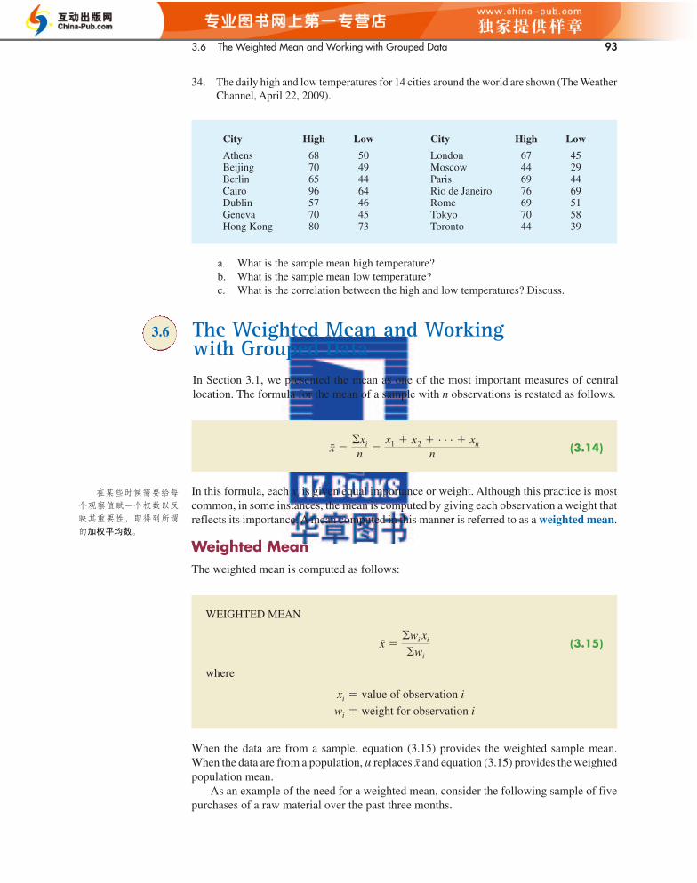
34. The daily high and low temperatures for 14 cities around the world are shown (The WeatherChannel, April 22, 2009).
(3.14)x ��xi
n �x1 � x2 � . . . � xn
n
WEIGHTED MEAN
(3.15)
where
xi �
wi �
value of observation i
weight for observation i
x ��wi
xi
�wi
Weighted Mean
The weighted mean is computed as follows:
When the data are from a sample, equation (3.15) provides the weighted sample mean.When the data are from a population, μ replaces and equation (3.15) provides the weightedpopulation mean.
As an example of the need for a weighted mean, consider the following sample of fivepurchases of a raw material over the past three months.
x
a. What is the sample mean high temperature?b. What is the sample mean low temperature?c. What is the correlation between the high and low temperatures? Discuss.
In Section 3.1, we presented the mean as one of the most important measures of centrallocation. The formula for the mean of a sample with n observations is restated as follows.
CH003.qxd 8/16/10 6:28 PM Page 125
在某些时候需要给每
个观察值赋一个权数以反
映其重要性,即得到所谓
的加权平均数。
City High Low City High Low
Athens 68 50 London 67 45Beijing 70 49 Moscow 44 29Berlin 65 44 Paris 69 44Cairo 96 64 Rio de Janeiro 76 69Dublin 57 46 Rome 69 51Geneva 70 45 Tokyo 70 58Hong Kong 80 73 Toronto 44 39
3.6 The Weighted Mean and Working with Grouped Data
In this formula, each xi is given equal importance or weight. Although this practice is mostcommon, in some instances, the mean is computed by giving each observation a weight thatreflects its importance. A mean computed in this manner is referred to as a weighted mean.
94 Chapter 3 Descriptive Statistics: Numerical Measures
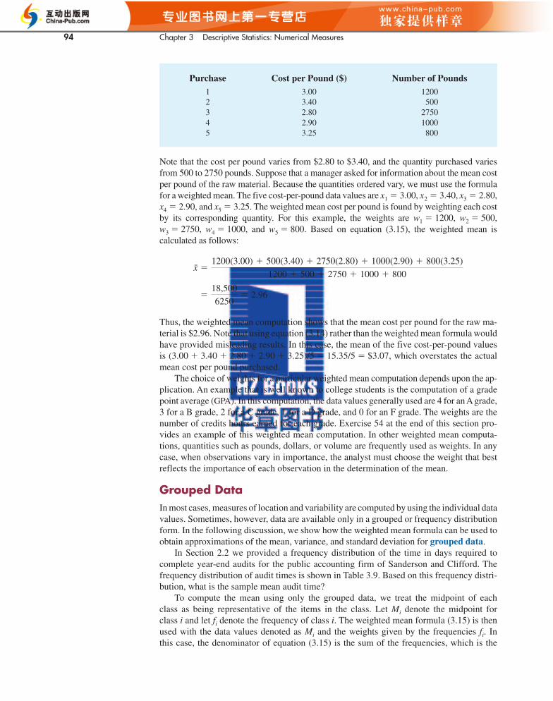
Purchase Cost per Pound ($) Number of Pounds1 3.00 12002 3.40 5003 2.80 27504 2.90 10005 3.25 800
Note that the cost per pound varies from $2.80 to $3.40, and the quantity purchased variesfrom 500 to 2750 pounds. Suppose that a manager asked for information about the mean costper pound of the raw material. Because the quantities ordered vary, we must use the formulafor a weighted mean. The five cost-per-pound data values are x1 � 3.00, x2 � 3.40, x3 � 2.80,x4 � 2.90, and x5 � 3.25. The weighted mean cost per pound is found by weighting each costby its corresponding quantity. For this example, the weights are w1 � 1200, w2 � 500,w3 � 2750, w4 � 1000, and w5 � 800. Based on equation (3.15), the weighted mean iscalculated as follows:
Thus, the weighted mean computation shows that the mean cost per pound for the raw ma-terial is $2.96. Note that using equation (3.14) rather than the weighted mean formula wouldhave provided misleading results. In this case, the mean of the five cost-per-pound valuesis (3.00 � 3.40 � 2.80 � 2.90 � 3.25)/5 � 15.35/5 � $3.07, which overstates the actualmean cost per pound purchased.
The choice of weights for a particular weighted mean computation depends upon the ap-plication. An example that is well known to college students is the computation of a gradepoint average (GPA). In this computation, the data values generally used are 4 for an A grade,3 for a B grade, 2 for a C grade, 1 for a D grade, and 0 for an F grade. The weights are thenumber of credits hours earned for each grade. Exercise 54 at the end of this section pro-vides an example of this weighted mean computation. In other weighted mean computa-tions, quantities such as pounds, dollars, or volume are frequently used as weights. In anycase, when observations vary in importance, the analyst must choose the weight that bestreflects the importance of each observation in the determination of the mean.
Grouped Data
In most cases, measures of location and variability are computed by using the individual datavalues. Sometimes, however, data are available only in a grouped or frequency distributionform. In the following discussion, we show how the weighted mean formula can be used toobtain approximations of the mean, variance, and standard deviation for grouped data.
In Section 2.2 we provided a frequency distribution of the time in days required tocomplete year-end audits for the public accounting firm of Sanderson and Clifford. Thefrequency distribution of audit times is shown in Table 3.9. Based on this frequency distri-bution, what is the sample mean audit time?
To compute the mean using only the grouped data, we treat the midpoint of each class as being representative of the items in the class. Let Mi denote the midpoint for class i and let fi denote the frequency of class i. The weighted mean formula (3.15) is thenused with the data values denoted as Mi and the weights given by the frequencies fi. In this case, the denominator of equation (3.15) is the sum of the frequencies, which is the
�18,500
6250� 2.96
x �1200(3.00) � 500(3.40) � 2750(2.80) � 1000(2.90) � 800(3.25)
1200 � 500 � 2750 � 1000 � 800
CH003.qxd 8/16/10 6:28 PM Page 126
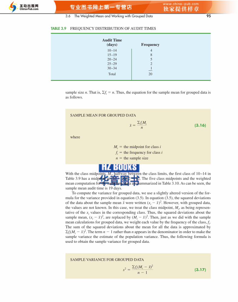
3.6 The Weighted Mean and Working with Grouped Data 95
SAMPLE MEAN FOR GROUPED DATA
(3.16)
where
Mi �
fi �
n �
the midpoint for class i
the frequency for class i
the sample size
x �� fi
Mi
n
sample size n. That is, �fi � n. Thus, the equation for the sample mean for grouped data isas follows.
SAMPLE VARIANCE FOR GROUPED DATA
(3.17)s2 �� fi
(Mi � x)2
n � 1
With the class midpoints, Mi, halfway between the class limits, the first class of 10–14 inTable 3.9 has a midpoint at (10 � 14)/2 � 12. The five class midpoints and the weightedmean computation for the audit time data are summarized in Table 3.10. As can be seen, thesample mean audit time is 19 days.
To compute the variance for grouped data, we use a slightly altered version of the for-mula for the variance provided in equation (3.5). In equation (3.5), the squared deviationsof the data about the sample mean were written (xi � )2. However, with grouped data,the values are not known. In this case, we treat the class midpoint, Mi, as being represen-tative of the xi values in the corresponding class. Thus, the squared deviations about thesample mean, (xi � )2, are replaced by (Mi � )2. Then, just as we did with the samplemean calculations for grouped data, we weight each value by the frequency of the class, fi.The sum of the squared deviations about the mean for all the data is approximated by�fi(Mi � )2. The term n � 1 rather than n appears in the denominator in order to make thesample variance the estimate of the population variance. Thus, the following formula isused to obtain the sample variance for grouped data.
x
xx
xx
TABLE 3.9 FREQUENCY DISTRIBUTION OF AUDIT TIMES
CH003.qxd 8/16/10 6:28 PM Page 127
Audit Time(days) Frequency10–14 415–19 820–24 525–29 230–34 1
Total 20
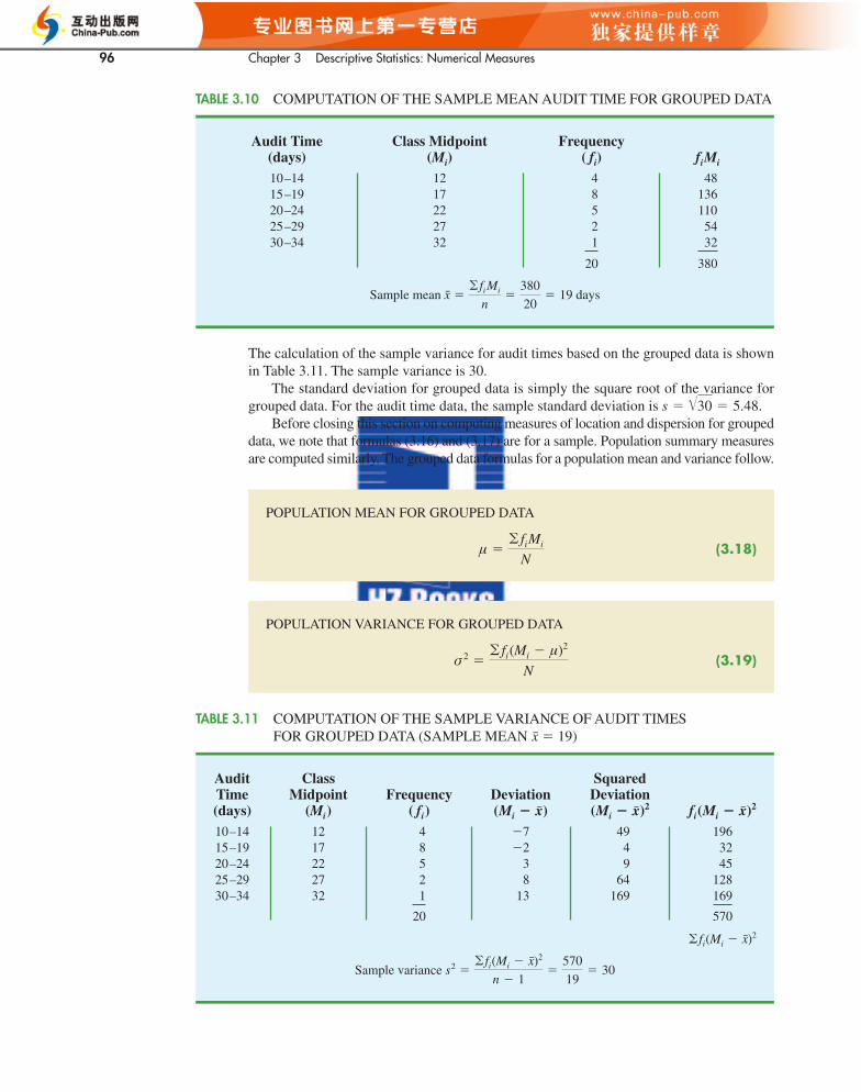
96 Chapter 3 Descriptive Statistics: Numerical Measures
CH003.qxd 8/16/10 6:28 PM Page 128
Audit Time Class Midpoint Frequency(days) (Mi) ( fi) fiMi
10–14 12 4 4815–19 17 8 13620–24 22 5 11025–29 27 2 5430–34 32 1 32
20 380
Sample mean x �� fiMi
n�
380
20� 19 days
TABLE 3.10 COMPUTATION OF THE SAMPLE MEAN AUDIT TIME FOR GROUPED DATA
Audit Class SquaredTime Midpoint Frequency Deviation Deviation(days) (Mi) ( fi) ( ) ( )2 fi( )2
10–14 12 4 �7 49 19615–19 17 8 �2 4 3220–24 22 5 3 9 4525–29 27 2 8 64 12830–34 32 1 13 169 169
20 570
Sample variance s2 �� fi(Mi � x)2
n � 1�
570
19� 30
� fi(Mi � x)2
Mi � xMi � xMi � x
TABLE 3.11 COMPUTATION OF THE SAMPLE VARIANCE OF AUDIT TIMES FOR GROUPED DATA (SAMPLE MEAN � 19)x
POPULATION MEAN FOR GROUPED DATA
(3.18)μ �� fi Mi
N
POPULATION VARIANCE FOR GROUPED DATA
(3.19)σ 2 �� fi (Mi � μ)2
N
The calculation of the sample variance for audit times based on the grouped data is shownin Table 3.11. The sample variance is 30.
The standard deviation for grouped data is simply the square root of the variance forgrouped data. For the audit time data, the sample standard deviation is
Before closing this section on computing measures of location and dispersion for groupeddata, we note that formulas (3.16) and (3.17) are for a sample. Population summary measuresare computed similarly. The grouped data formulas for a population mean and variance follow.
s � �30 � 5.48.
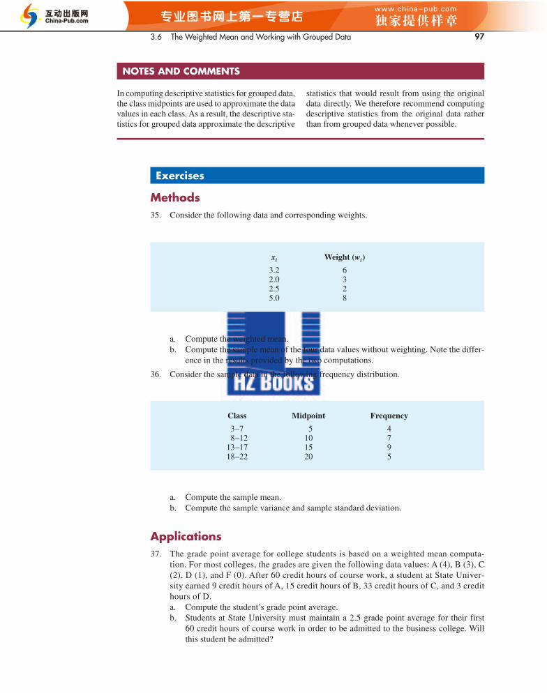
3.6 The Weighted Mean and Working with Grouped Data 97
Exercises
Methods
35. Consider the following data and corresponding weights.
xi Weight (wi)
3.2 62.0 32.5 25.0 8
a. Compute the weighted mean.b. Compute the sample mean of the four data values without weighting. Note the differ-
ence in the results provided by the two computations.
36. Consider the sample data in the following frequency distribution.
a. Compute the sample mean.b. Compute the sample variance and sample standard deviation.
Applications
37. The grade point average for college students is based on a weighted mean computa-tion. For most colleges, the grades are given the following data values: A (4), B (3), C(2), D (1), and F (0). After 60 credit hours of course work, a student at State Univer-sity earned 9 credit hours of A, 15 credit hours of B, 33 credit hours of C, and 3 credithours of D.a. Compute the student’s grade point average.b. Students at State University must maintain a 2.5 grade point average for their first
60 credit hours of course work in order to be admitted to the business college. Will this student be admitted?
Class Midpoint Frequency
3–7 5 48–12 10 7
13–17 15 918–22 20 5
NOTES AND COMMENTS
In computing descriptive statistics for grouped data,the class midpoints are used to approximate the datavalues in each class. As a result, the descriptive sta-tistics for grouped data approximate the descriptive
statistics that would result from using the originaldata directly. We therefore recommend computingdescriptive statistics from the original data ratherthan from grouped data whenever possible.
CH003.qxd 8/16/10 6:28 PM Page 129
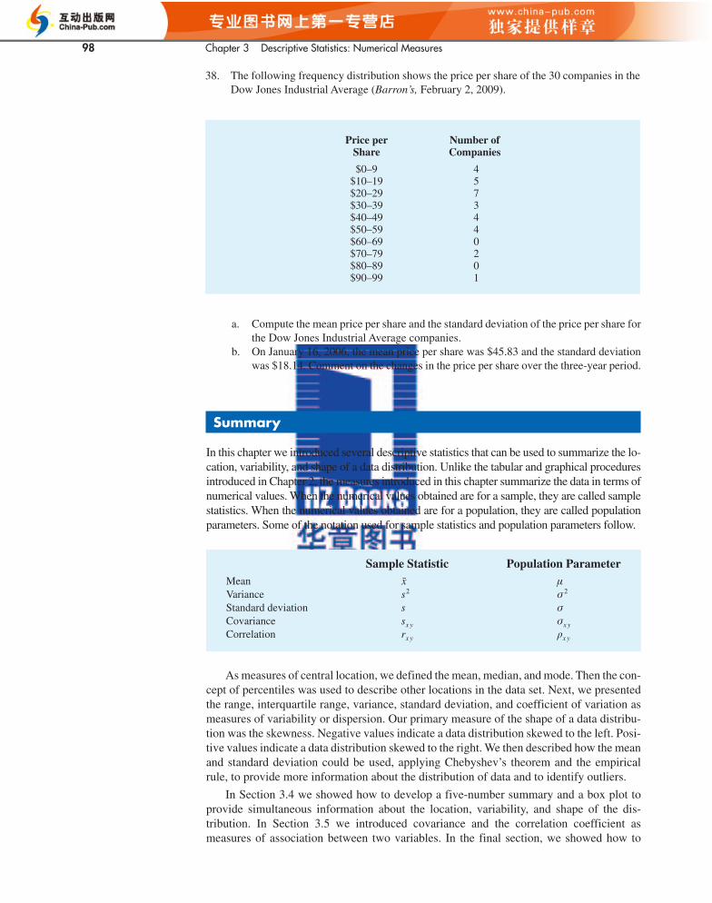
98 Chapter 3 Descriptive Statistics: Numerical Measures
38. The following frequency distribution shows the price per share of the 30 companies in theDow Jones Industrial Average (Barron’s, February 2, 2009).
Price per Number ofShare Companies
$0–9 4$10–19 5$20–29 7$30–39 3$40–49 4$50–59 4$60–69 0$70–79 2$80–89 0$90–99 1
CH003.qxd 8/16/10 6:28 PM Page 130
a. Compute the mean price per share and the standard deviation of the price per share forthe Dow Jones Industrial Average companies.
b. On January 16, 2006, the mean price per share was $45.83 and the standard deviationwas $18.14. Comment on the changes in the price per share over the three-year period.
Summary
In this chapter we introduced several descriptive statistics that can be used to summarize the lo-cation, variability, and shape of a data distribution. Unlike the tabular and graphical proceduresintroduced in Chapter 2, the measures introduced in this chapter summarize the data in terms ofnumerical values. When the numerical values obtained are for a sample, they are called samplestatistics. When the numerical values obtained are for a population, they are called populationparameters. Some of the notation used for sample statistics and population parameters follow.
Sample Statistic Population ParameterMean μVarianceStandard deviation s σCovariance s σCorrelation r �x yx y
x yx y
σ 2s2x
As measures of central location, we defined the mean, median, and mode. Then the con-cept of percentiles was used to describe other locations in the data set. Next, we presentedthe range, interquartile range, variance, standard deviation, and coefficient of variation asmeasures of variability or dispersion. Our primary measure of the shape of a data distribu-tion was the skewness. Negative values indicate a data distribution skewed to the left. Posi-tive values indicate a data distribution skewed to the right. We then described how the meanand standard deviation could be used, applying Chebyshev’s theorem and the empiricalrule, to provide more information about the distribution of data and to identify outliers.
In Section 3.4 we showed how to develop a five-number summary and a box plot toprovide simultaneous information about the location, variability, and shape of the dis-tribution. In Section 3.5 we introduced covariance and the correlation coefficient asmeasures of association between two variables. In the final section, we showed how to
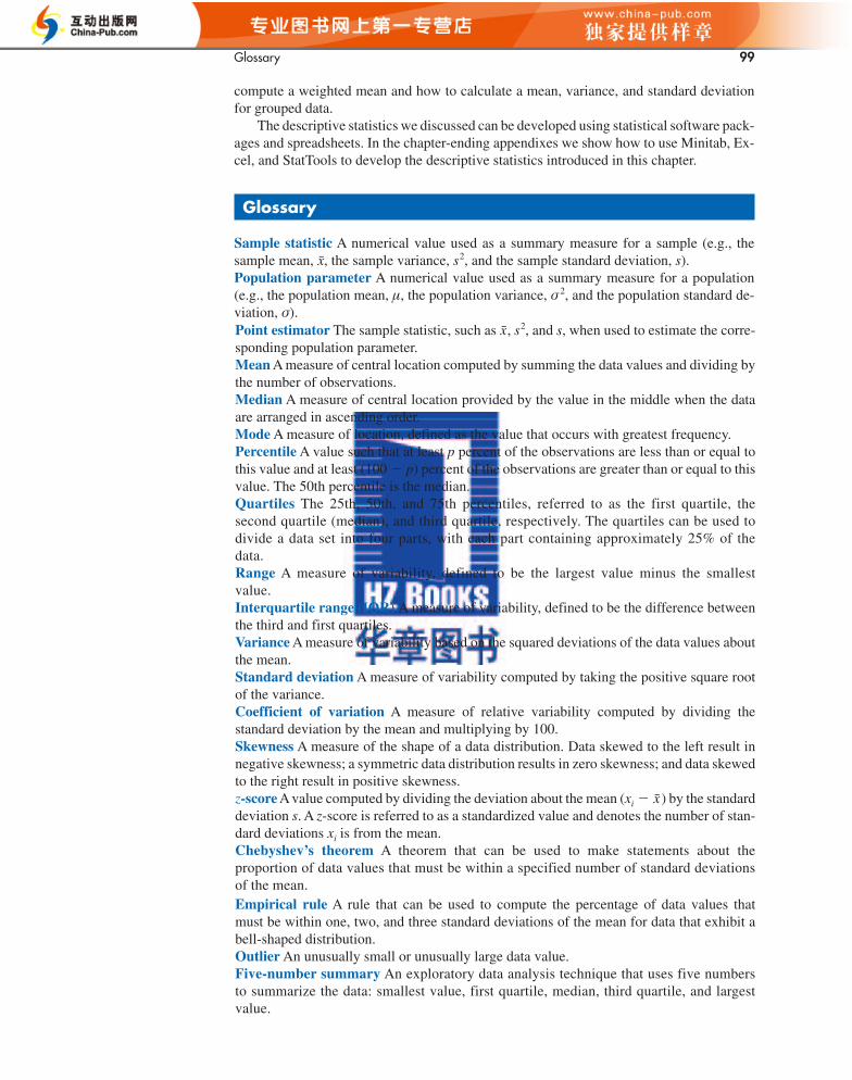
Glossary 99
compute a weighted mean and how to calculate a mean, variance, and standard deviationfor grouped data.
The descriptive statistics we discussed can be developed using statistical software pack-ages and spreadsheets. In the chapter-ending appendixes we show how to use Minitab, Ex-cel, and StatTools to develop the descriptive statistics introduced in this chapter.
Glossary
Sample statistic A numerical value used as a summary measure for a sample (e.g., thesample mean, , the sample variance, s2, and the sample standard deviation, s).Population parameter A numerical value used as a summary measure for a population(e.g., the population mean, μ, the population variance, σ 2, and the population standard de-viation, σ).
x
CH003.qxd 8/16/10 6:28 PM Page 131
Point estimator The sample statistic, such as , s2, and s, when used to estimate the corre-sponding population parameter.Mean A measure of central location computed by summing the data values and dividing bythe number of observations.Median A measure of central location provided by the value in the middle when the dataare arranged in ascending order.Mode A measure of location, defined as the value that occurs with greatest frequency.Percentile A value such that at least p percent of the observations are less than or equal tothis value and at least (100 � p) percent of the observations are greater than or equal to thisvalue. The 50th percentile is the median.Quartiles The 25th, 50th, and 75th percentiles, referred to as the first quartile, thesecond quartile (median), and third quartile, respectively. The quartiles can be used todivide a data set into four parts, with each part containing approximately 25% of thedata.Range A measure of variability, defined to be the largest value minus the smallest value.Interquartile range (IQR) A measure of variability, defined to be the difference betweenthe third and first quartiles.Variance A measure of variability based on the squared deviations of the data values aboutthe mean.Standard deviation A measure of variability computed by taking the positive square rootof the variance.Coefficient of variation A measure of relative variability computed by dividing thestandard deviation by the mean and multiplying by 100.Skewness A measure of the shape of a data distribution. Data skewed to the left result innegative skewness; a symmetric data distribution results in zero skewness; and data skewedto the right result in positive skewness.z-score A value computed by dividing the deviation about the mean (xi � ) by the standarddeviation s. A z-score is referred to as a standardized value and denotes the number of stan-dard deviations xi is from the mean.Chebyshev’s theorem A theorem that can be used to make statements about theproportion of data values that must be within a specified number of standard deviationsof the mean.
x
x
Empirical rule A rule that can be used to compute the percentage of data values thatmust be within one, two, and three standard deviations of the mean for data that exhibit abell-shaped distribution.Outlier An unusually small or unusually large data value.Five-number summary An exploratory data analysis technique that uses five numbersto summarize the data: smallest value, first quartile, median, third quartile, and largestvalue.
100 Chapter 3 Descriptive Statistics: Numerical Measures
Box plot A graphical summary of data based on a five-number summary.Covariance A measure of linear association between two variables. Positive values indi-cate a positive relationship; negative values indicate a negative relationship.Correlation coefficient A measure of linear association between two variables that takeson values between �1 and �1. Values near �1 indicate a strong positive linear relation-ship; values near �1 indicate a strong negative linear relationship; and values near zeroindicate the lack of a linear relationship.Weighted mean The mean obtained by assigning each observation a weight that reflects itsimportance.Grouped data Data available in class intervals as summarized by a frequency distribution.Individual values of the original data are not available.
CH003.qxd 8/16/10 6:28 PM Page 132
Key Formulas
Sample Mean
(3.1)
Population Mean
(3.2)
Interquartile Range
(3.3)
Population Variance
(3.4)
Sample Variance
(3.5)
Standard Deviation
(3.6)
(3.7)
Coefficient of Variation
(3.8)
z-Score
(3.9)zi �xi � x
s
�Standard deviation
Mean� 100�%
Population standard deviation � σ � �σ 2
Sample standard deviation � s � �s2
s2 ��(xi � x)2
n � 1
σ 2 ��(xi � μ)2
N
IQR � Q3 � Q1
μ ��xi
N
x ��xi
n
Sample Covariance
(3.10)sxy ��(xi � x)(
yi � y)
n � 1
Supplementary Exercises 101
Population Covariance
(3.11)
Pearson Product Moment Correlation Coefficient: Sample Data
(3.12)rxy �sxy
sx sy
CH003.qxd 8/16/10 6:28 PM Page 133
Pearson Product Moment Correlation Coefficient: Population Data
(3.13)
Supplementary Exercises
39. According to an annual consumer spending survey, the average monthly Bank of AmericaVisa credit card charge was $1838 (U.S. Airways Attaché Magazine, December 2003). A sample of monthly credit card charges provides the following data.
236 1710 1351 825 7450316 4135 1333 1584 387991 3396 170 1428 1688
a. Compute the mean and median.b. Compute the first and third quartiles.c. Compute the range and interquartile range.d. Compute the variance and standard deviation.
σxy ��(xi � μx)(
yi � μy)
N
�xy �σxy
σxσy
Weighted Mean
(3.15)
Sample Mean for Grouped Data
(3.16)
Sample Variance for Grouped Data
(3.17)
Population Mean for Grouped Data
(3.18)
Population Variance for Grouped Data
(3.19)σ 2 �� fi (Mi � μ)2
N
μ �� fi Mi
N
s2 �� fi (Mi � x)2
n � 1
x �� fi Mi
n
x ��wi xi
�wi

102 Chapter 3 Descriptive Statistics: Numerical Measures
e. The skewness measure for these data is 2.12. Comment on the shape of this distribu-tion. Is it the shape you would expect? Why or why not?
f. Do the data contain outliers?
40. The U.S. Census Bureau provides statistics on family life in the United States, includingthe age at the time of first marriage, current marital status, and size of household (U.S. Census Bureau website, March 20, 2006). The following data show the age at thetime of first marriage for a sample of men and a sample of women.
CH003.qxd 8/16/10 6:28 PM Page 134
Men 26 23 28 25 27 30 26 35 28
21 24 27 29 30 27 32 27 25
Women 20 28 23 30 24 29 26 25
22 22 25 23 27 26 19
a. Determine the median age at the time of first marriage for men and women.
b. Compute the first and third quartiles for both men and women.
c. Twenty-five years ago the median age at the time of first marriage was 25 for men and
22 for women. What insight does this information provide about the decision of when
to marry among young people today?
41. Small business owners often look to payroll service companies to handle their employee
payroll. Reasons are that small business owners face complicated tax regulations, and
penalties for employment tax errors are costly. According to the Internal Revenue Service,
26% of all small business employment tax returns contained errors that resulted in a tax
penalty to the owner (The Wall Street Journal, January 30, 2006). The tax penalty for a
sample of 20 small business owners follows:
820 270 450 1010 890 700 1350 350 300 1200
390 730 2040 230 640 350 420 270 370 620
a. What is the mean tax penalty for improperly filed employment tax returns?
b. What is the standard deviation?
c. Is the highest penalty, $2040, an outlier?
d. What are some of the advantages of a small business owner hiring a payroll service
company to handle employee payroll services, including the employment tax returns?
42. The National Association of Realtors reported the median home price in the United States
and the increase in median home price over a five-year period (The Wall Street Journal, Jan-
uary 16, 2006). Use the sample home prices shown here to answer the following questions.
995.9 48.8 175.0 263.5 298.0 218.9 209.0
628.3 111.0 212.9 92.6 2325.0 958.0 212.5
a. What is the sample median home price?
b. In January 2001, the National Association of Realtors reported a median home price
of $139,300 in the United States. What was the percentage increase in the median
home price over the five-year period?
c. What are the first quartile and the third quartile for the sample data?
d. Provide a five-number summary for the home prices.
e. Do the data contain any outliers?
f. What is the mean home price for the sample? Why does the National Association of
Realtors prefer to use the median home price in its reports?
Case Problem 1 Pelican StoresPelican Stores, a division of National Clothing, is a chain of women’s apparel stores
operating throughout the country. The chain recently ran a promotion in which discount
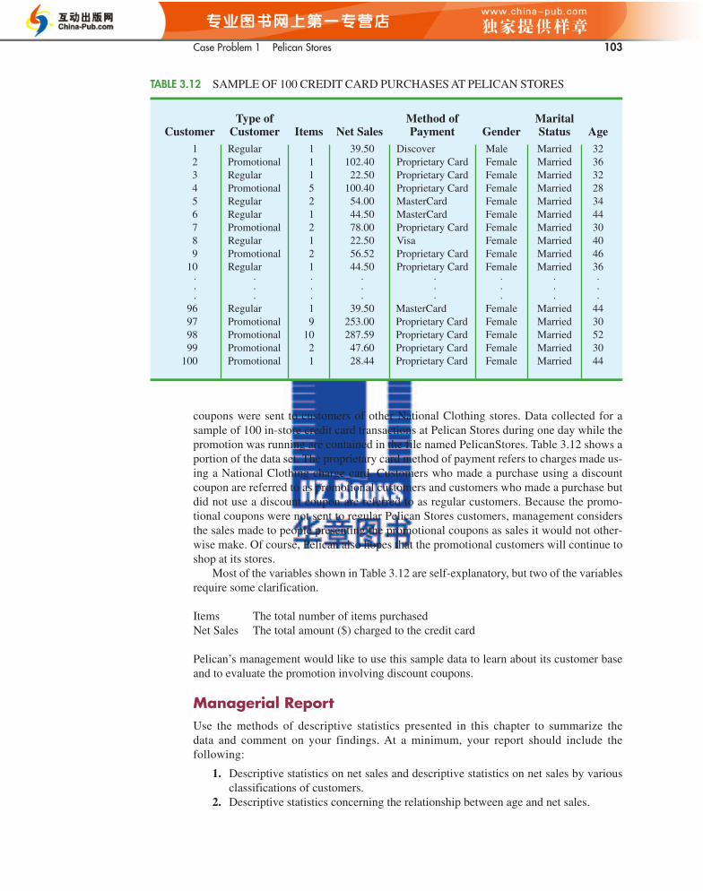
Case Problem 1 Pelican Stores 103
coupons were sent to customers of other National Clothing stores. Data collected for asample of 100 in-store credit card transactions at Pelican Stores during one day while thepromotion was running are contained in the file named PelicanStores. Table 3.12 shows aportion of the data set. The proprietary card method of payment refers to charges made us-ing a National Clothing charge card. Customers who made a purchase using a discountcoupon are referred to as promotional customers and customers who made a purchase butdid not use a discount coupon are referred to as regular customers. Because the promo-tional coupons were not sent to regular Pelican Stores customers, management considersthe sales made to people presenting the promotional coupons as sales it would not other-wise make. Of course, Pelican also hopes that the promotional customers will continue toshop at its stores.
Most of the variables shown in Table 3.12 are self-explanatory, but two of the variablesrequire some clarification.
Items The total number of items purchasedNet Sales The total amount ($) charged to the credit card
Pelican’s management would like to use this sample data to learn about its customer baseand to evaluate the promotion involving discount coupons.
Managerial Report
Use the methods of descriptive statistics presented in this chapter to summarize the data and comment on your findings. At a minimum, your report should include thefollowing:
1. Descriptive statistics on net sales and descriptive statistics on net sales by variousclassifications of customers.
2. Descriptive statistics concerning the relationship between age and net sales.
Type of Method of MaritalCustomer Customer Items Net Sales Payment Gender Status Age
1 Regular 1 39.50 Discover Male Married 322 Promotional 1 102.40 Proprietary Card Female Married 363 Regular 1 22.50 Proprietary Card Female Married 324 Promotional 5 100.40 Proprietary Card Female Married 285 Regular 2 54.00 MasterCard Female Married 346 Regular 1 44.50 MasterCard Female Married 447 Promotional 2 78.00 Proprietary Card Female Married 308 Regular 1 22.50 Visa Female Married 409 Promotional 2 56.52 Proprietary Card Female Married 46
10 Regular 1 44.50 Proprietary Card Female Married 36. . . . . . . .. . . . . . . .. . . . . . . .
96 Regular 1 39.50 MasterCard Female Married 4497 Promotional 9 253.00 Proprietary Card Female Married 3098 Promotional 10 287.59 Proprietary Card Female Married 5299 Promotional 2 47.60 Proprietary Card Female Married 30
100 Promotional 1 28.44 Proprietary Card Female Married 44
TABLE 3.12 SAMPLE OF 100 CREDIT CARD PURCHASES AT PELICAN STORES
CH003.qxd 8/16/10 6:28 PM Page 139
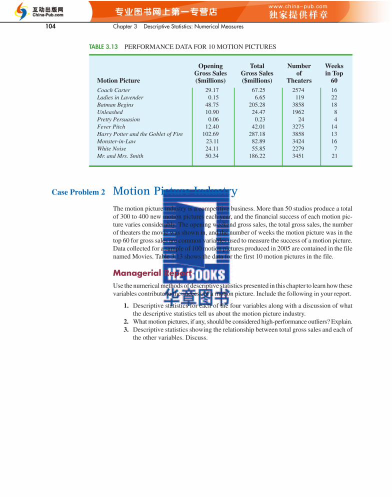
104 Chapter 3 Descriptive Statistics: Numerical Measures
Opening Total Number Weeks Gross Sales Gross Sales of in Top
Motion Picture ($millions) ($millions) Theaters 60Coach Carter 29.17 67.25 2574 16Ladies in Lavender 0.15 6.65 119 22Batman Begins 48.75 205.28 3858 18Unleashed 10.90 24.47 1962 8Pretty Persuasion 0.06 0.23 24 4Fever Pitch 12.40 42.01 3275 14Harry Potter and the Goblet of Fire 102.69 287.18 3858 13Monster-in-Law 23.11 82.89 3424 16White Noise 24.11 55.85 2279 7Mr. and Mrs. Smith 50.34 186.22 3451 21
TABLE 3.13 PERFORMANCE DATA FOR 10 MOTION PICTURES
Case Problem 2 Motion Picture IndustryThe motion picture industry is a competitive business. More than 50 studios produce a totalof 300 to 400 new motion pictures each year, and the financial success of each motion pic-ture varies considerably. The opening weekend gross sales, the total gross sales, the numberof theaters the movie was shown in, and the number of weeks the motion picture was in thetop 60 for gross sales are common variables used to measure the success of a motion picture.Data collected for a sample of 100 motion pictures produced in 2005 are contained in the filenamed Movies. Table 3.13 shows the data for the first 10 motion pictures in the file.
Managerial Report
Use the numerical methods of descriptive statistics presented in this chapter to learn how thesevariables contribute to the success of a motion picture. Include the following in your report.
1. Descriptive statistics for each of the four variables along with a discussion of whatthe descriptive statistics tell us about the motion picture industry.
2. What motion pictures, if any, should be considered high-performance outliers? Explain.3. Descriptive statistics showing the relationship between total gross sales and each of
the other variables. Discuss.
CH003.qxd 8/16/10 6:28 PM Page 140