Descriptive Statistics (Part 2) Chapter44 Standardized Data Percentiles, Quartiles and Box Plots Grouped Data Skewness and Kurtosis McGraw-Hill/Irwin Copyright

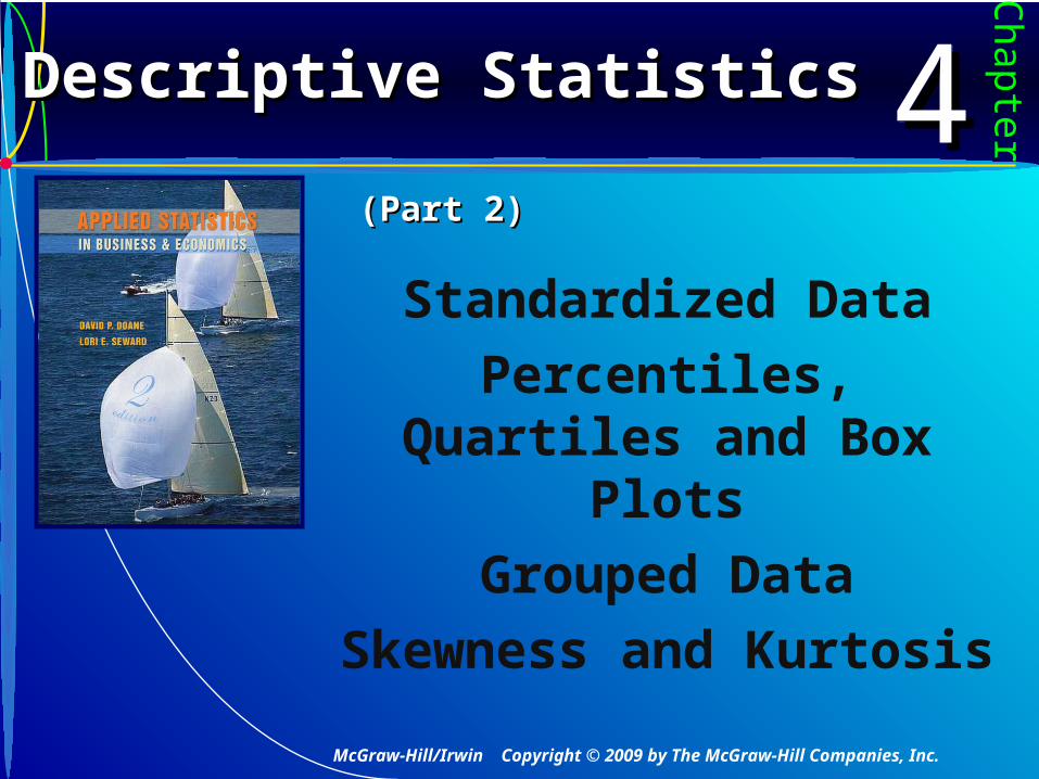
Descriptive Statistics Descriptive Statistics (Part 2)(Part 2)

Chapter4444

Standardized Data

Percentiles, Quartiles and Box Plots

Grouped Data

Skewness and Kurtosis

McGraw-Hill/Irwin Copyright © 2009 by The McGraw-Hill Companies, Inc.

4B-2

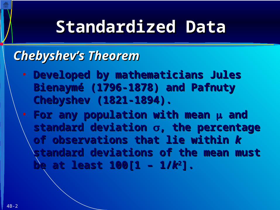
• For any population with mean For any population with mean and standard and standard deviation deviation , the percentage of observations , the percentage of observations that lie within that lie within kk standard deviations of the standard deviations of the mean must be at least 100[1 – 1/mean must be at least 100[1 – 1/kk22]. ].

• Developed by mathematicians Jules BienaymDeveloped by mathematicians Jules Bienayméé (1796-1878) and Pafnuty Chebyshev (1821-(1796-1878) and Pafnuty Chebyshev (1821-1894).1894).

Standardized DataStandardized DataStandardized DataStandardized Data

Chebyshev’s TheoremChebyshev’s Theorem

4B-3

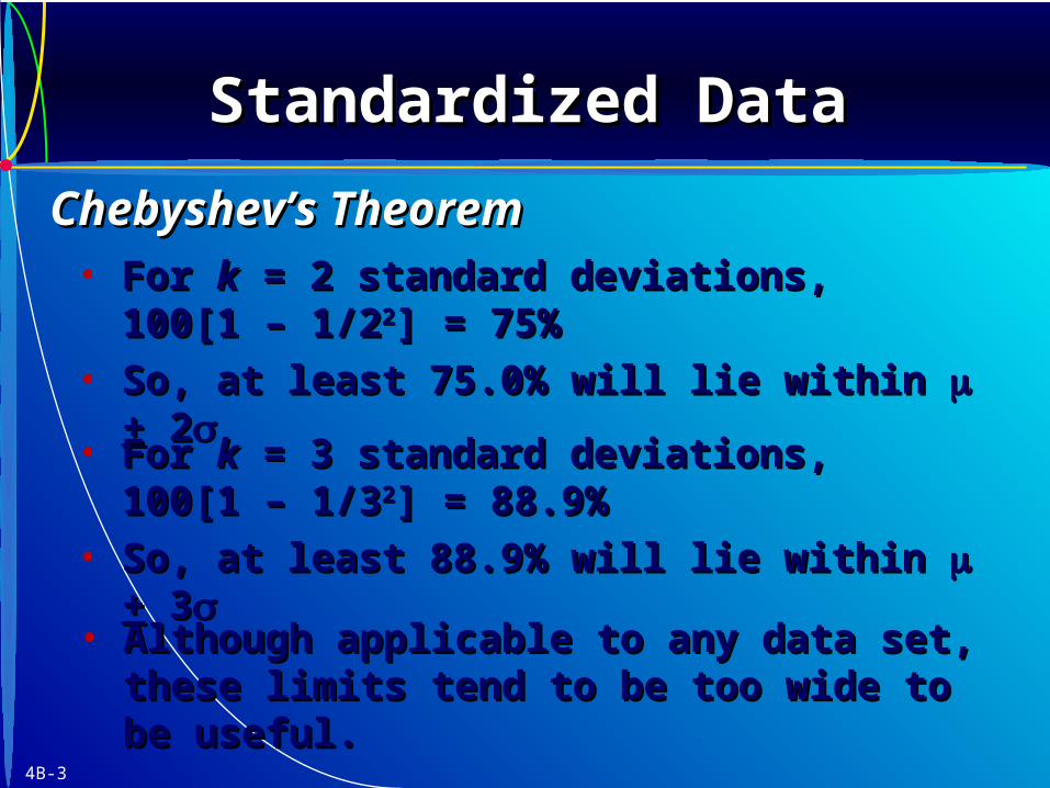
• For For kk = 2 standard deviations, = 2 standard deviations, 100[1 – 1/2100[1 – 1/222] = 75%] = 75%

• So, at least 75.0% will lie within So, at least 75.0% will lie within ++ 2 2

• For For kk = 3 standard deviations, = 3 standard deviations, 100[1 – 1/3100[1 – 1/322] = 88.9%] = 88.9%

• So, at least 88.9% will lie within So, at least 88.9% will lie within ++ 3 3

• Although applicable to any data set, these Although applicable to any data set, these limits tend to be too wide to be useful.limits tend to be too wide to be useful.


Chebyshev’s TheoremChebyshev’s Theorem

4B-4

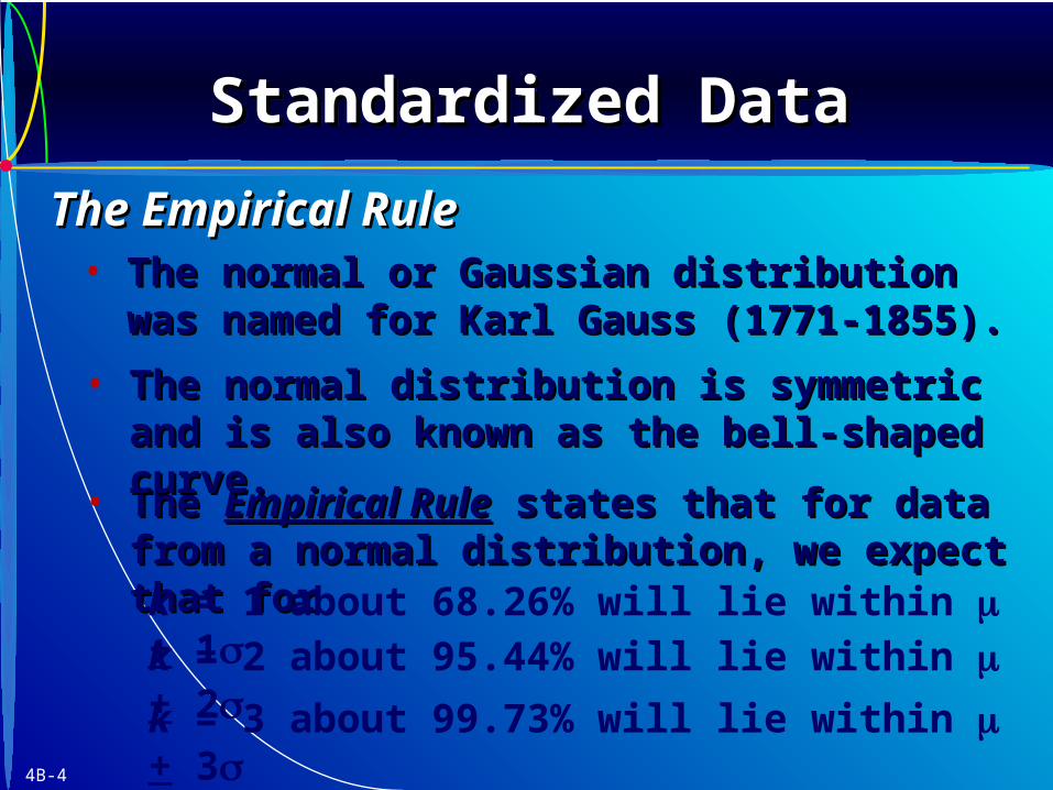
• The The Empirical RuleEmpirical Rule states that for data from a states that for data from a normal distribution, we expect that fornormal distribution, we expect that for

• The normal or Gaussian distribution was The normal or Gaussian distribution was named for Karl Gauss (1771-1855).named for Karl Gauss (1771-1855).

• The normal distribution is symmetric and is The normal distribution is symmetric and is also known as the bell-shaped curve.also known as the bell-shaped curve.

k = 1 about 68.26% will lie within + 1k = 2 about 95.44% will lie within + 2

k = 3 about 99.73% will lie within + 3


The Empirical RuleThe Empirical Rule

4B-5

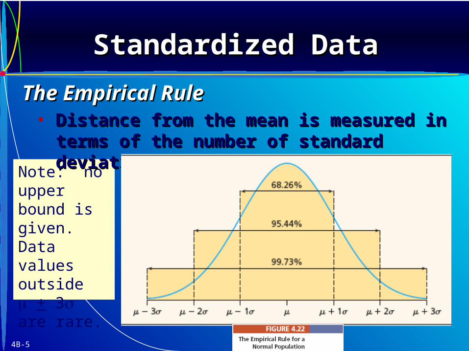
Note: no upper bound is given. Data values outside + 3 are rare.

• Distance from the mean is measured in terms Distance from the mean is measured in terms of the number of standard deviations.of the number of standard deviations.



4B-6

• If 80 students take an exam, how many will score If 80 students take an exam, how many will score within 2 standard deviations of the mean?within 2 standard deviations of the mean?

• Assuming exam scores follow a normal Assuming exam scores follow a normal distribution, the empirical rule statesdistribution, the empirical rule statesabout 95.44% will lie within about 95.44% will lie within ++ 2 2

so 95.44% x 80 so 95.44% x 80 76 students will score 76 students will score ++ 2 2 from from ..

• How many students will score more than 2 How many students will score more than 2 standard deviations from the mean?standard deviations from the mean?


Example: Exam ScoresExample: Exam Scores

4B-7

• UnusualUnusual observations are those that lie beyond observations are those that lie beyond

++ 2 2..• OutliersOutliers are observations that lie beyond are observations that lie beyond

++ 3 3..


Unusual ObservationsUnusual Observations

4B-8

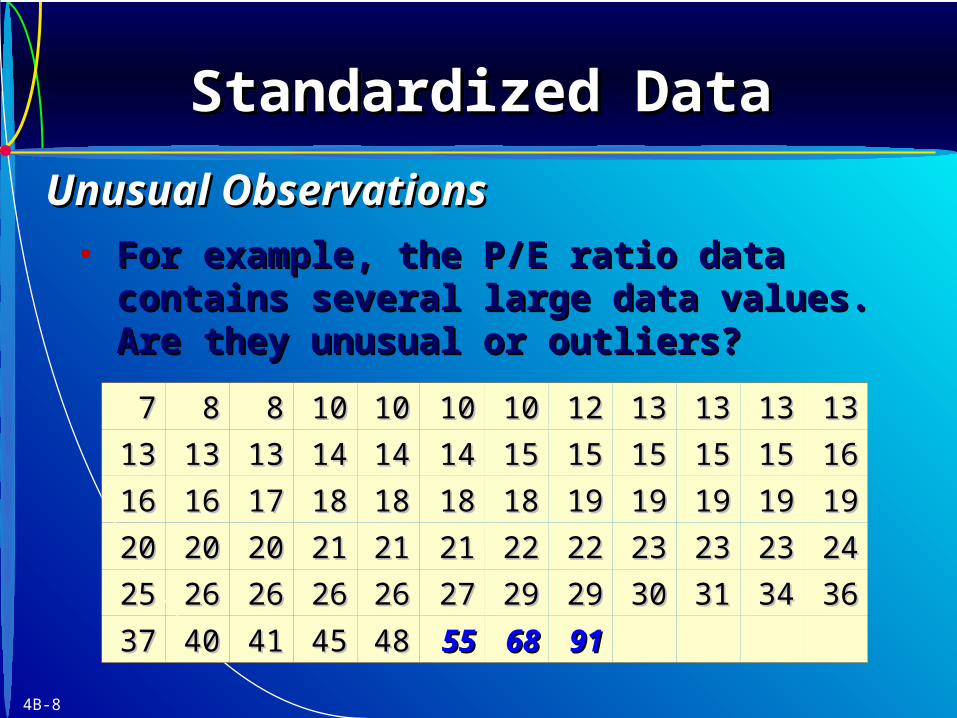
• For example, the P/E ratio data contains For example, the P/E ratio data contains several large data values. Are they unusual or several large data values. Are they unusual or outliers?outliers?

77 88 88 1010 1010 1010 1010 1212 1313 1313 1313 1313

1313 1313 1313 1414 1414 1414 1515 1515 1515 1515 1515 1616

1616 1616 1717 1818 1818 1818 1818 1919 1919 1919 1919 1919

2020 2020 2020 2121 2121 2121 2222 2222 2323 2323 2323 2424

2525 2626 2626 2626 2626 2727 2929 2929 3030 3131 3434 3636

3737 4040 4141 4545 4848 5555 6868 9191


Unusual ObservationsUnusual Observations

4B-9

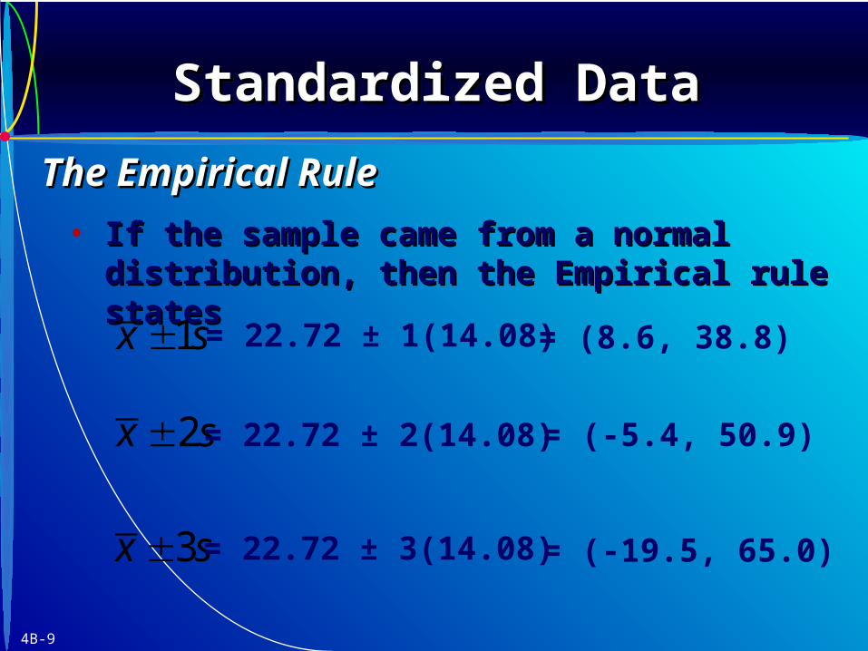
• If the sample came from a normal distribution, If the sample came from a normal distribution, then the Empirical rule statesthen the Empirical rule states

1x s = 22.72 ± 1(14.08)

2x s = 22.72 ± 2(14.08)

3x s = 22.72 ± 3(14.08)



= (8.6, 38.8)

= (-5.4, 50.9)

= (-19.5, 65.0)

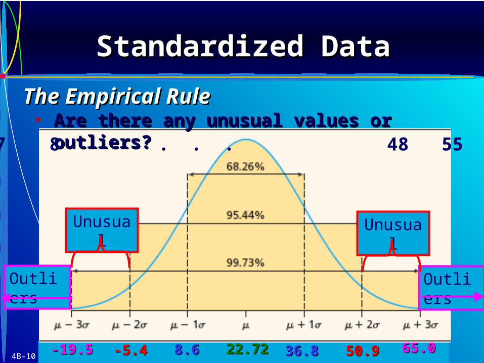
4B-1022.7222.72 36.836.88.68.6 50.950.9-5.4-5.4 65.065.0-19.5-19.5



Outliers Outliers

UnusualUnusual

• Are there any unusual values or outliers?Are there any unusual values or outliers?7 8 . . . 48 55 68 91

4B-11

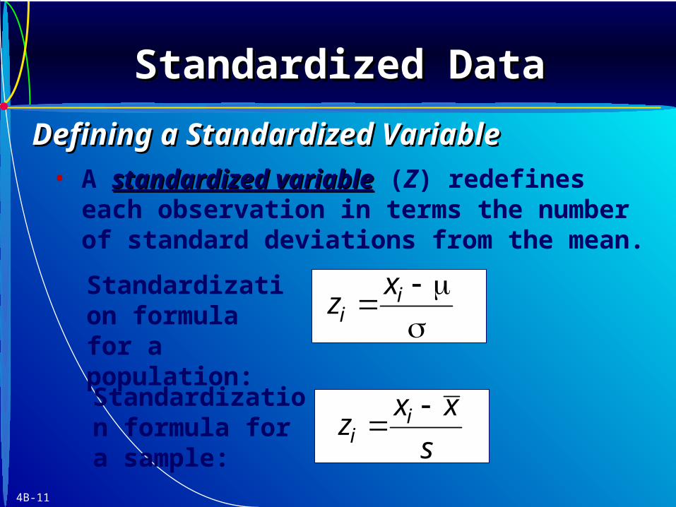
• A standardized variablestandardized variable (Z) redefines each observation in terms the number of standard deviations from the mean.

iix

z

Standardization formula for a population:

Standardization formula for a sample:

iix x

zs


Defining a Standardized VariableDefining a Standardized Variable

4B-12

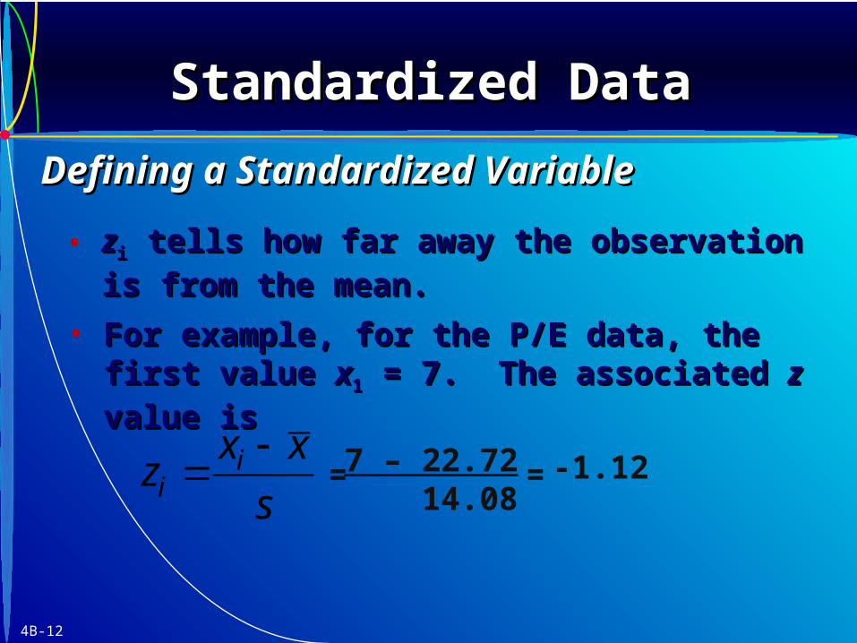
• zzii tells how far away the observation is from tells how far away the observation is from

the mean. the mean.

iix x

zs

= 7 – 22.72

14.08= -1.12



• For example, for the P/E data, the first value For example, for the P/E data, the first value xx11

= 7. The associated = 7. The associated zz value is value is

4B-13

iix x

zs

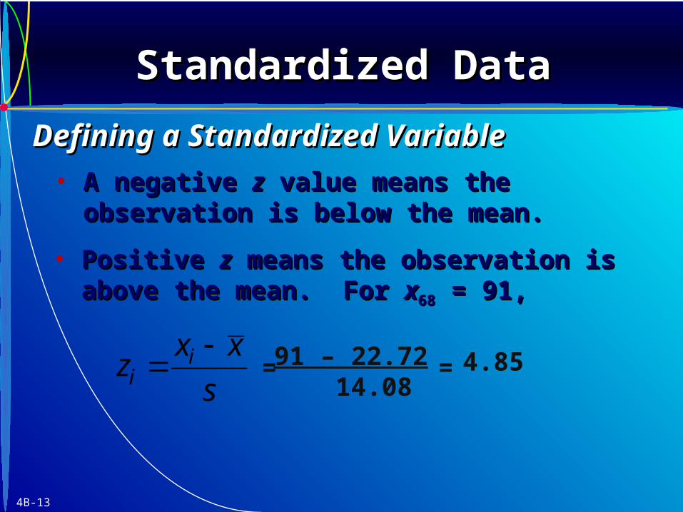
= 91 – 22.72

14.08= 4.85

• A negative A negative zz value means the observation is value means the observation is below the mean.below the mean.



• Positive Positive zz means the observation is above the means the observation is above the mean. For mean. For xx6868 = 91, = 91,

4B-14

• Here are the standardized Here are the standardized zz values for the P/E values for the P/E data:data:



• What do you conclude for these three values?What do you conclude for these three values?

4B-15

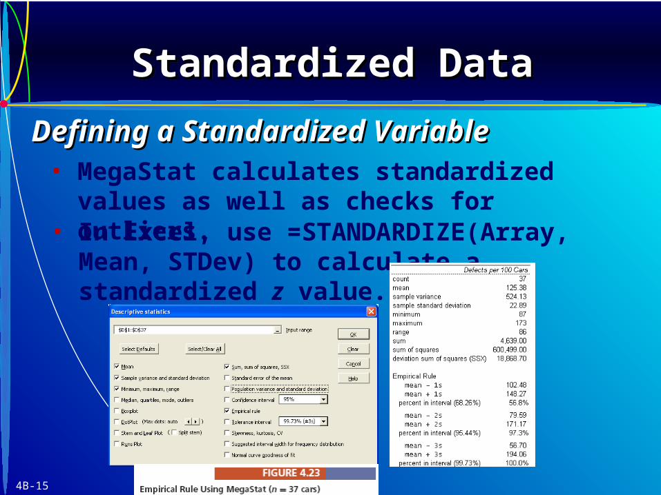
• In Excel, use =STANDARDIZE(Array, Mean, STDev) to calculate a standardized z value.

• MegaStat calculates standardized values as well as checks for outliers.



4B-16

• What do we do with outliers in a data set?What do we do with outliers in a data set?

• If due to erroneous data, then discard.If due to erroneous data, then discard.

• An outrageous observation (one completely An outrageous observation (one completely outside of an expected range) is certainly outside of an expected range) is certainly invalid.invalid.

• Recognize unusual data points and outliers Recognize unusual data points and outliers and their potential impact on your study.and their potential impact on your study.

• Research books and articles on how to handle Research books and articles on how to handle outliers.outliers.


OutliersOutliers

4B-17

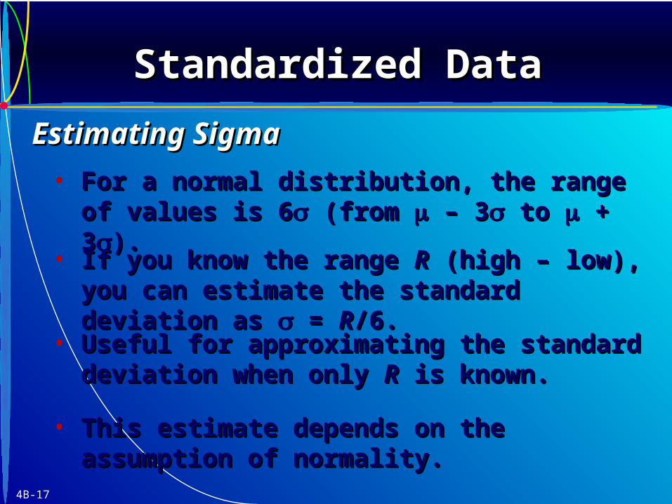
• For a normal distribution, the range of values For a normal distribution, the range of values is 6is 6 (from (from – 3 – 3 to to + 3 + 3).).

• If you know the range If you know the range RR (high – low), you can (high – low), you can estimate the standard deviation as estimate the standard deviation as = = RR/6./6.

• Useful for approximating the standard Useful for approximating the standard deviation when only deviation when only RR is known. is known.

• This estimate depends on the assumption of This estimate depends on the assumption of normality.normality.


Estimating SigmaEstimating Sigma

4B-18

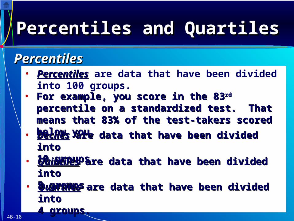
• PercentilesPercentiles are data that have been divided into 100 groups.

• For example, you score in the 83For example, you score in the 83rdrd percentile on a percentile on a standardized test. That means that 83% of the test-standardized test. That means that 83% of the test-takers scored below you. takers scored below you.

• DecilesDeciles are data that have been divided into are data that have been divided into 10 groups.10 groups.

• QuintilesQuintiles are data that have been divided into are data that have been divided into 5 groups.5 groups.

• QuartilesQuartiles are data that have been divided into are data that have been divided into 4 groups.4 groups.

Percentiles and QuartilesPercentiles and QuartilesPercentiles and QuartilesPercentiles and Quartiles

PercentilesPercentiles

4B-19

• Percentiles are used to establish benchmarksbenchmarks for comparison purposes (e.g., health care, manufacturing and banking industries use 5, 25, 50, 75 and 90 percentiles).

• Quartiles (25, 50, and 75 percent) are commonly used to assess financial performance and stock portfolios.

• Percentiles are used in employee merit evaluation and salary benchmarking.


PercentilesPercentiles

4B-20

• QuartilesQuartiles are scale points that divide the sorted data into four groups of approximately equal size.

• The three values that separate the four groups are called Q1, Q2, and Q3, respectively.

Q1 Q2 Q3

Lower 25% | Second 25% | Third 25% | Upper 25%


QuartilesQuartiles

4B-21

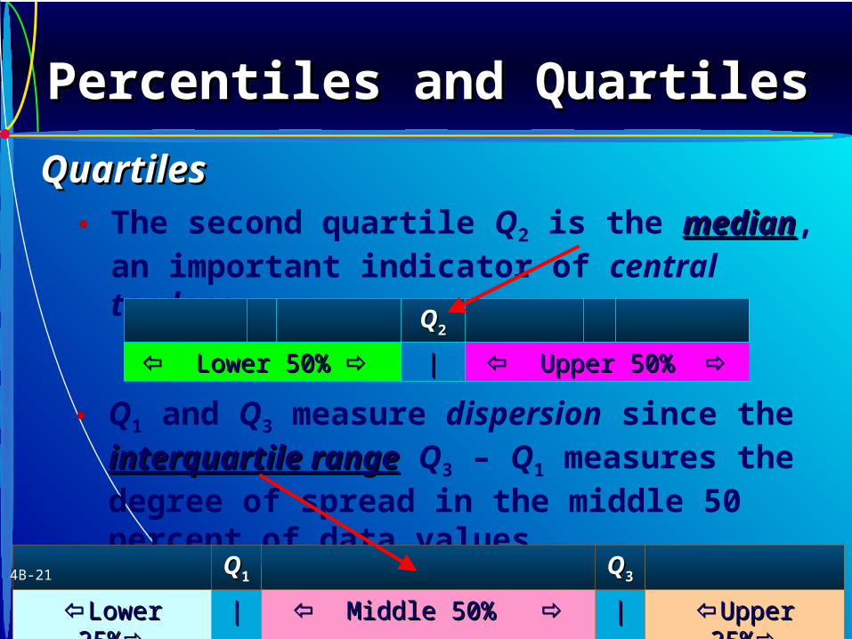
• The second quartile Q2 is the medianmedian, an important indicator of central tendency.

• Q1 and Q3 measure dispersion since the

interquartile rangeinterquartile range Q3 – Q1 measures the degree of spread in the middle 50 percent of data values.

QQ22

Lower 50% Lower 50% || Upper 50% Upper 50%

QQ11 QQ33

Lower 25%Lower 25% || Middle 50% Middle 50% || Upper 25%Upper 25%


QuartilesQuartiles

4B-21

4B-22

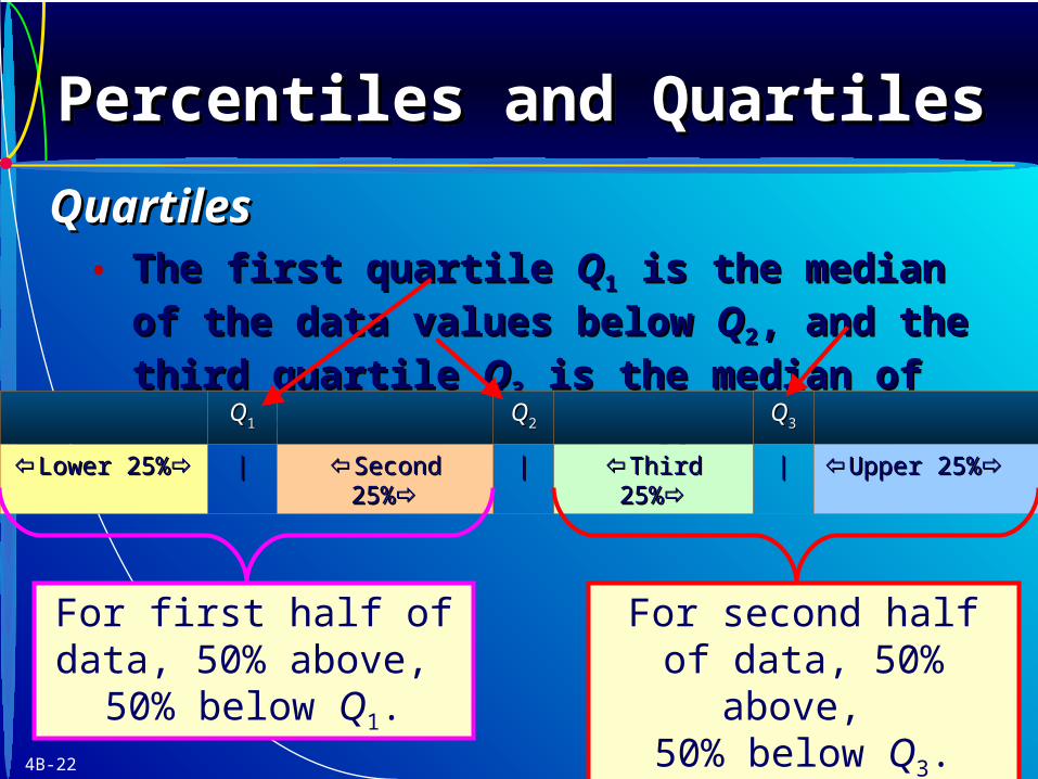
• The first quartile The first quartile QQ11 is the median of the data is the median of the data

values below values below QQ22, and the third quartile , and the third quartile QQ33 is is

the median of the data values above the median of the data values above QQ22..QQ11 QQ22 QQ33

Lower 25%Lower 25% || Second 25%Second 25% || Third 25%Third 25% || Upper 25%Upper 25%

For first half of data, 50% above,

50% below Q1.

For second half of data, 50% above,

50% below Q3.


QuartilesQuartiles

4B-23

• Depending on Depending on nn, the quartiles , the quartiles QQ11,,QQ22, and , and QQ33

may be members of the data set or may lie may be members of the data set or may lie betweenbetween two of the sorted data values. two of the sorted data values.


QuartilesQuartiles

4B-24

• For small data sets, find quartiles using method of mediansmethod of medians:

Step 1. Sort the observations.

Step 2. Find the median Q2.

Step 3. Find the median of the data values that lie belowbelow Q2.

Step 4. Find the median of the data values that lie aboveabove Q2.


Method of MediansMethod of Medians

4B-25

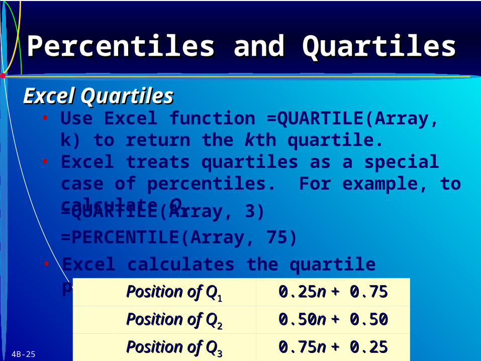
• Use Excel function =QUARTILE(Array, k) to return the kth quartile.

=QUARTILE(Array, 3)

=PERCENTILE(Array, 75)

• Excel treats quartiles as a special case of percentiles. For example, to calculate Q3

• Excel calculates the quartile positions as:

Position of QPosition of Q11 0.250.25n n + 0.75+ 0.75




Excel QuartilesExcel Quartiles

4B-26

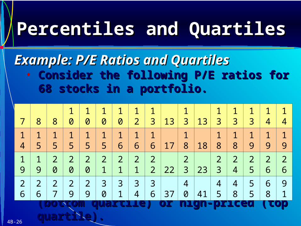
• Consider the following P/E ratios for 68 stocks Consider the following P/E ratios for 68 stocks in a portfolio. in a portfolio.

• Use quartiles to define benchmarks for stocks Use quartiles to define benchmarks for stocks that are low-priced (bottom quartile) or high-that are low-priced (bottom quartile) or high-priced (top quartile).priced (top quartile).

7 8 8 10 10 10 10 12 13 13 13 13 13 13 13 14 14

14 15 15 15 15 15 16 16 16 17 18 18 18 18 19 19 19

19 19 20 20 20 21 21 21 22 22 23 23 23 24 25 26 26

26 26 27 29 29 30 31 34 36 37 40 41 45 48 55 68 91


Example: P/E Ratios and QuartilesExample: P/E Ratios and Quartiles

4B-27

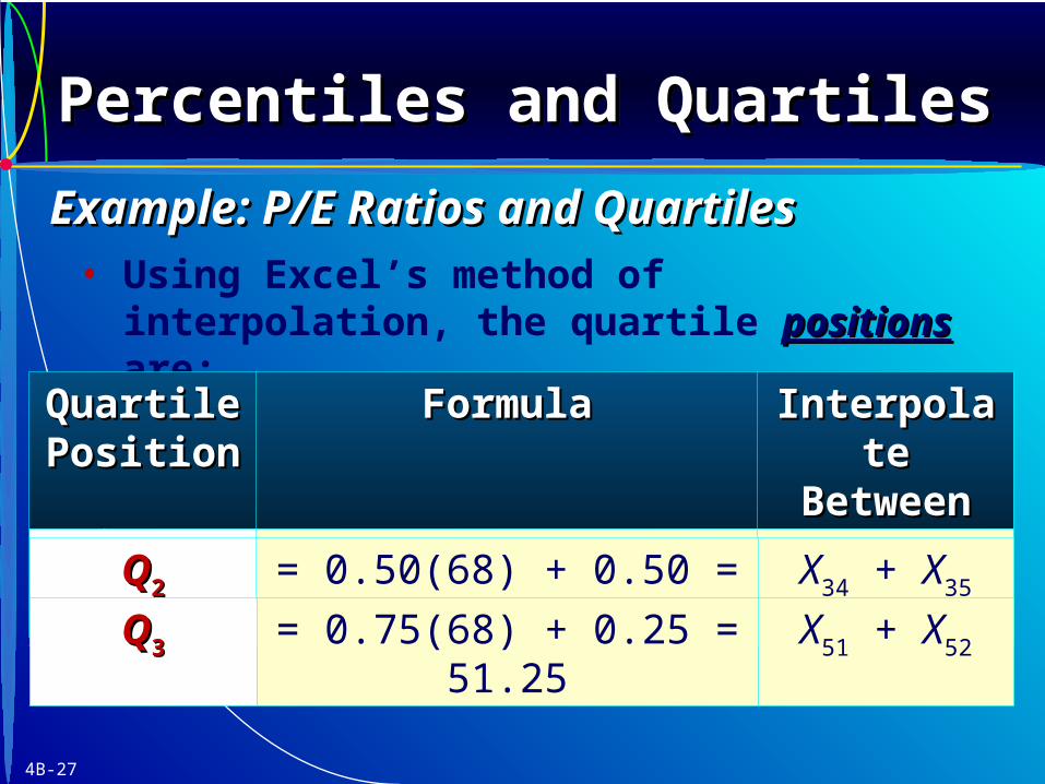
• Using Excel’s method of interpolation, the quartile positionspositions are:

Quartile Quartile PositionPosition

FormulaFormula Interpolate Interpolate BetweenBetween

QQ11= 0.25(68) + 0.75 = 17.75 X17 + X18



QQ22= 0.50(68) + 0.50 = 34.50 X34 + X35

QQ33= 0.75(68) + 0.25 = 51.25 X51 + X52

4B-28

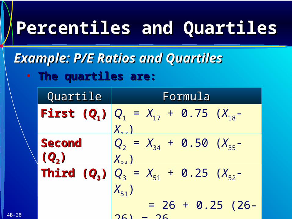
• The quartiles are:The quartiles are:

QuartileQuartile FormulaFormula

First (First (QQ11)) Q1 = X17 + 0.75 (X18-X17)

= 14 + 0.75 (14-14) = 14



Second (Second (QQ22)) Q2 = X34 + 0.50 (X35-X34)

= 19 + 0.50 (19-19) = 19Third (Third (QQ33)) Q3 = X51 + 0.25 (X52-X51)

= 26 + 0.25 (26-26) = 26

4B-29

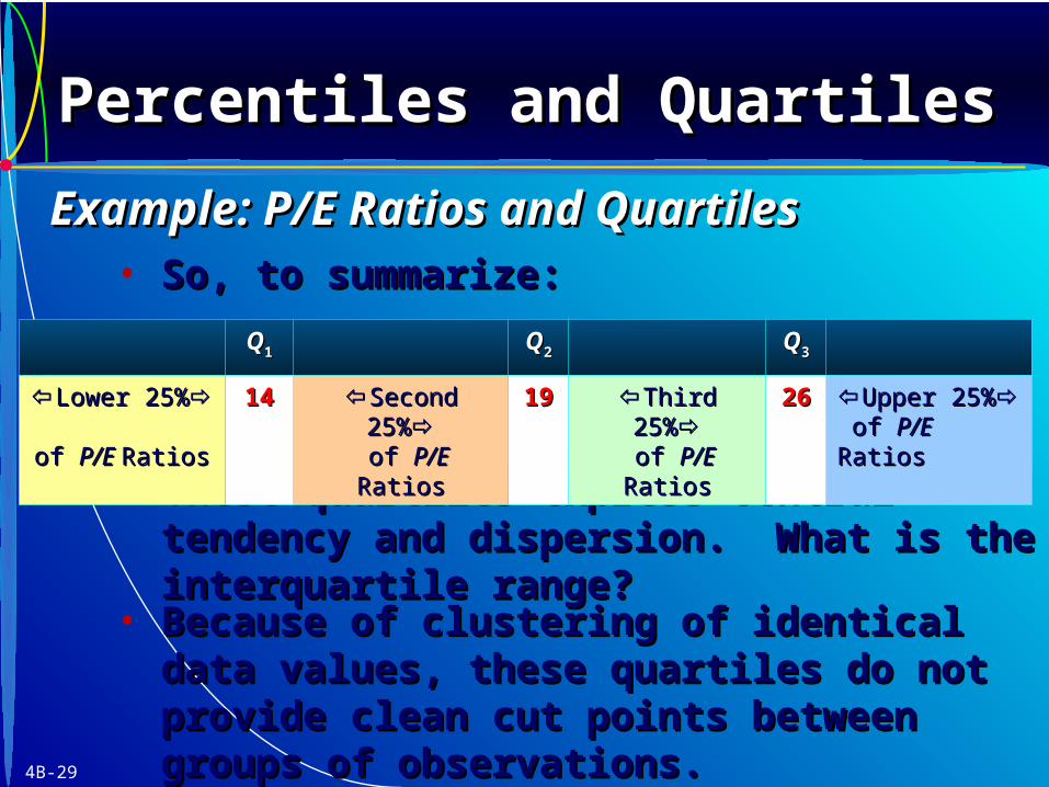
• So, to summarize:So, to summarize:

• These quartiles express central tendency and These quartiles express central tendency and dispersion. What is the interquartile range?dispersion. What is the interquartile range?

QQ11 QQ22 QQ33

Lower 25%Lower 25% of of P/E P/E RatiosRatios

1414 Second 25%Second 25% of of P/EP/E Ratios Ratios

1919 Third 25%Third 25% of of P/EP/E Ratios Ratios

2626 Upper 25%Upper 25% of of P/EP/E Ratios Ratios

• Because of clustering of identical data values, Because of clustering of identical data values, these quartiles do not provide clean cut points these quartiles do not provide clean cut points between groups of observations.between groups of observations.



4B-30

Whether you use the method of Whether you use the method of medians or Excel, your quartiles will medians or Excel, your quartiles will

be about the same. Small be about the same. Small differences in calculation techniques differences in calculation techniques

typically do not lead to different typically do not lead to different conclusions in business applications.conclusions in business applications.


TipTip

4B-31

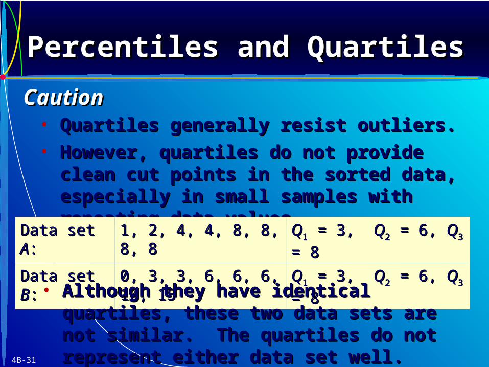
• Quartiles generally resist outliers.Quartiles generally resist outliers.

• However, quartiles do not provide clean cut However, quartiles do not provide clean cut points in the sorted data, especially in small points in the sorted data, especially in small samples with repeating data values.samples with repeating data values.

Data set Data set AA:: 1, 2, 4, 4, 8, 8, 8, 81, 2, 4, 4, 8, 8, 8, 8 QQ11 = 3, = 3, QQ22 = 6, = 6, QQ33 = 8 = 8

Data set Data set BB:: 0, 3, 3, 6, 6, 6, 10, 150, 3, 3, 6, 6, 6, 10, 15 QQ11 = 3, = 3, QQ22 = 6, = 6, QQ33 = 8 = 8

• Although they have identical quartiles, these Although they have identical quartiles, these two data sets are not similar. The quartiles do two data sets are not similar. The quartiles do not represent either data set well.not represent either data set well.


CautionCaution

4B-32

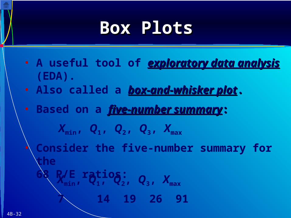
• A useful tool of exploratory data analysisexploratory data analysis (EDA).

• Also called a box-and-whisker plotbox-and-whisker plot..

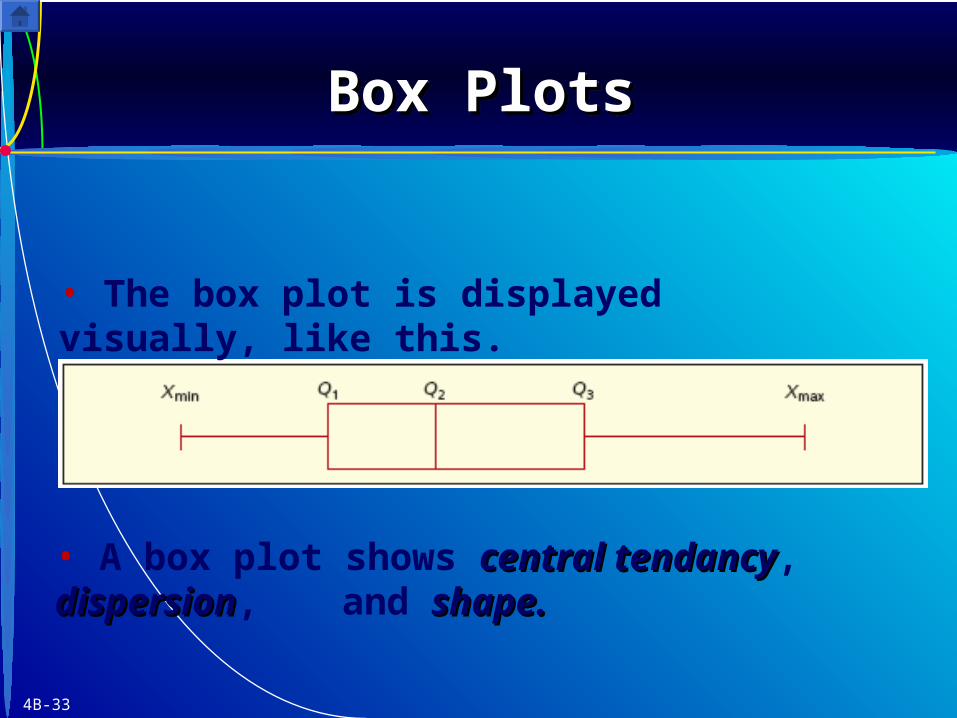
• Based on a five-number summaryfive-number summary::

Xmin, Q1, Q2, Q3, Xmax

• Consider the five-number summary for the 68 P/E ratios:

7 14 19 26 91

Xmin, Q1, Q2, Q3, Xmax

Box PlotsBox PlotsBox PlotsBox Plots

4B-33


• The box plot is displayed visually, like this.

• A box plot shows central tendancycentral tendancy, dispersiondispersion, and shape.shape.

4B-34

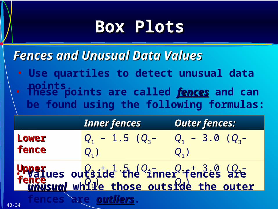
• Use quartiles to detect unusual data points.

• These points are called fencesfences and can be found using the following formulas:

Inner fencesInner fences Outer fences:Outer fences:

Lower fenceLower fence Q1 – 1.5 (Q3–Q1) Q1 – 3.0 (Q3–Q1)

Upper fenceUpper fence Q3 + 1.5 (Q3–Q1) Q3 + 3.0 (Q3–Q1)

• Values outside the inner fences are unusualunusual while those outside the outer fences are outliersoutliers.


Fences and Unusual Data ValuesFences and Unusual Data Values

4B-35

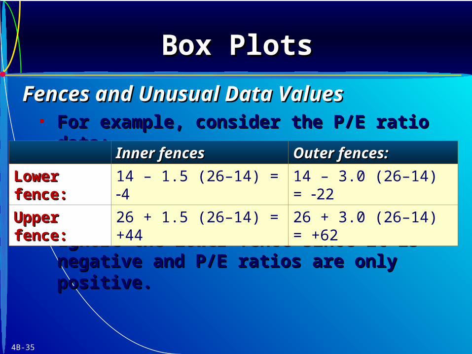
• For example, consider the P/E ratio data:For example, consider the P/E ratio data:

• Ignore the lower fence since it is negative and Ignore the lower fence since it is negative and P/E ratios are only positive. P/E ratios are only positive.

Inner fencesInner fences Outer fences:Outer fences:

Lower Lower fence:fence:

14 – 1.5 (26–14) = 4 14 – 3.0 (26–14) = 22

Upper fence:Upper fence: 26 + 1.5 (26–14) = +44 26 + 3.0 (26–14) = +62



4B-36

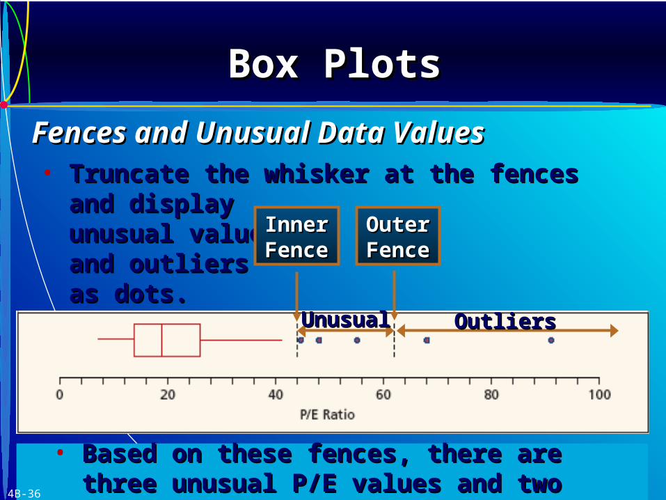
• Truncate the whisker at the fences and display Truncate the whisker at the fences and display

unusual values unusual values and outliers and outliers as dots.as dots.

Inner Inner FenceFence

OuterOuterFenceFence

UnusualUnusual OutliersOutliers



• Based on these fences, there are three Based on these fences, there are three unusual P/E values and two outliers.unusual P/E values and two outliers.4B-36

4B-37

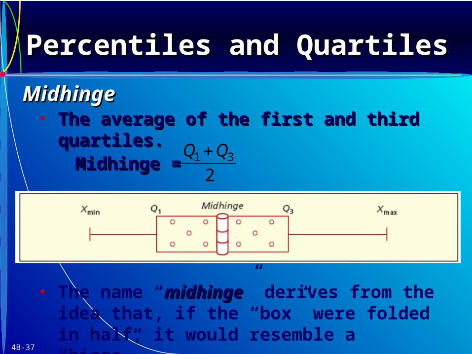
• The average of the first and third quartiles.The average of the first and third quartiles.

Midhinge = Midhinge = 1 3

2

Q Q

• The name “midhingemidhinge” derives from the idea that, if the “box” were folded in half, it would resemble a “hinge”..


MidhingeMidhinge

4B-38

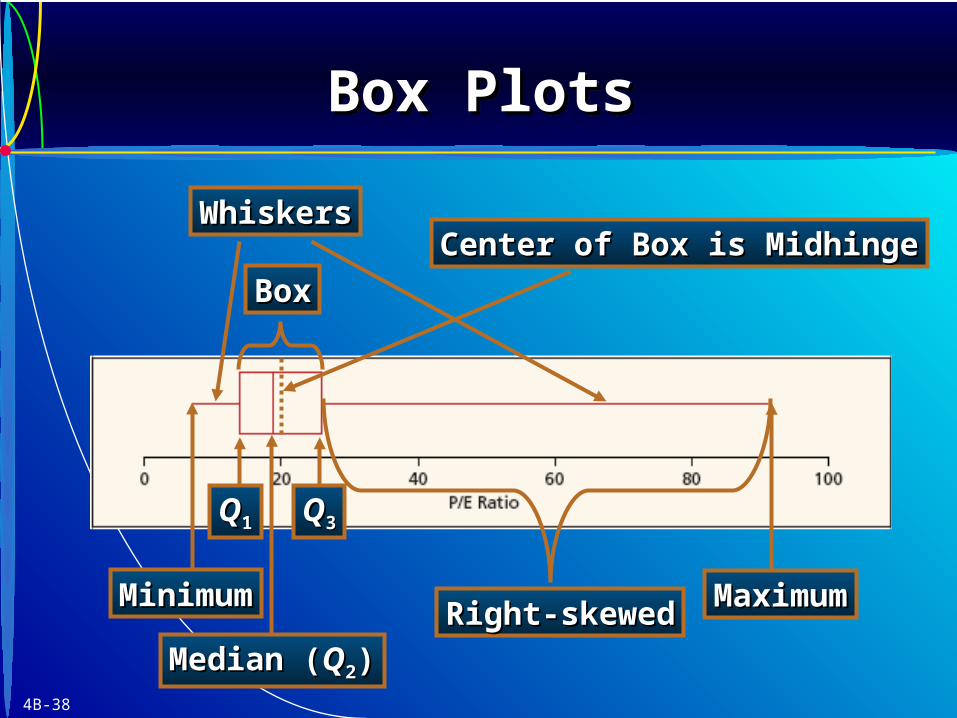
MinimumMinimum

Median (Median (QQ22))

MaximumMaximum

QQ11 QQ33

BoxBox

WhiskersWhiskers

Right-skewedRight-skewed

Center of Box is MidhingeCenter of Box is Midhinge


4B-39

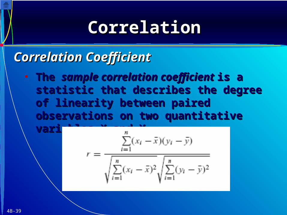
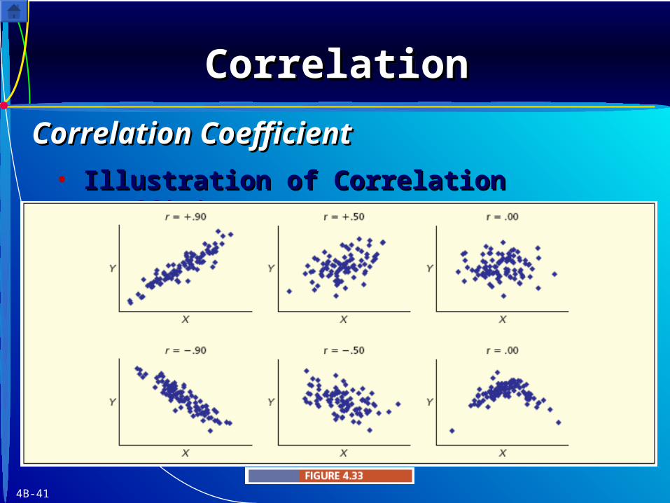
• The The sample correlation coefficient sample correlation coefficient is a statistic is a statistic that describes the degree of linearity between that describes the degree of linearity between paired observations on two quantitative paired observations on two quantitative variables X and Y.variables X and Y.

CorrelationCorrelationCorrelationCorrelation

Correlation CoefficientCorrelation Coefficient

4B-40

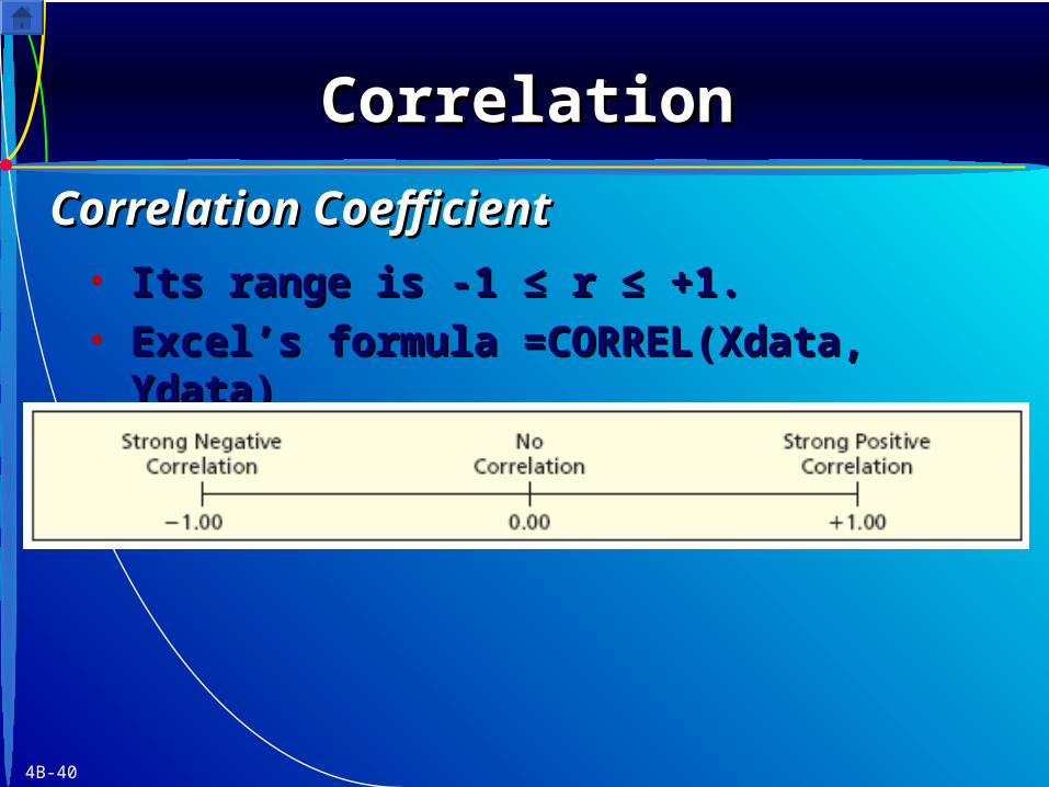
• Its range is -1 ≤ r ≤ +1.Its range is -1 ≤ r ≤ +1.• Excel’s formula =CORREL(Xdata, Ydata) Excel’s formula =CORREL(Xdata, Ydata)



4B-41

• Illustration of Correlation CoefficientsIllustration of Correlation Coefficients



4B-42

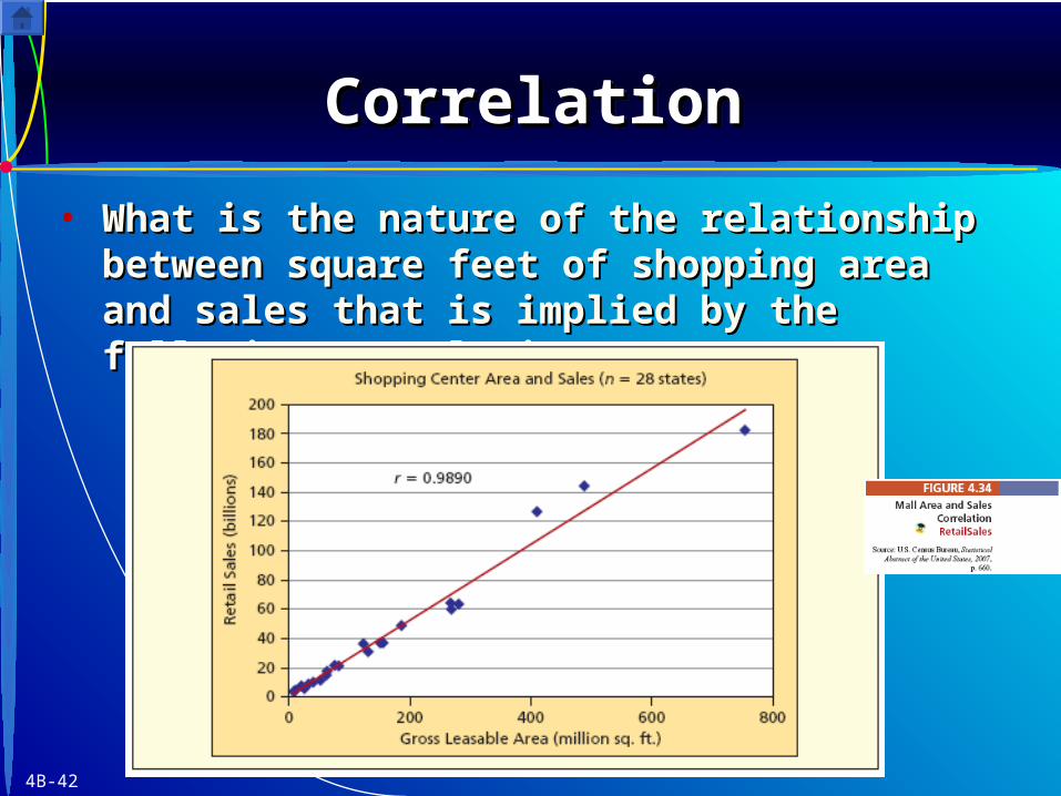
• What is the nature of the relationship between What is the nature of the relationship between square feet of shopping area and sales that is square feet of shopping area and sales that is implied by the following correlation?implied by the following correlation?


4B-43

• Although some information is lost, grouped Although some information is lost, grouped data are easier to display than raw data. data are easier to display than raw data.

• When bin limits are given, the mean and When bin limits are given, the mean and standard deviation can be estimated.standard deviation can be estimated.

• Accuracy of grouped estimates depend on Accuracy of grouped estimates depend on - the number of bins- the number of bins- distribution of data within bins- distribution of data within bins- bin frequencies- bin frequencies

Grouped DataGrouped DataGrouped DataGrouped Data

Nature of Grouped DataNature of Grouped Data

4B-44

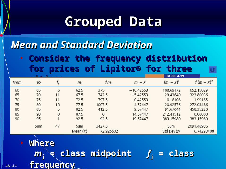
• Consider the frequency distribution for prices Consider the frequency distribution for prices of Lipitor® for three cities:of Lipitor® for three cities:


Mean and Standard DeviationMean and Standard Deviation

• WhereWhere mmjj = class midpoint = class midpoint ffjj = class frequency = class frequency

kk = number of classes = number of classes n n = sample size= sample size

4B-45

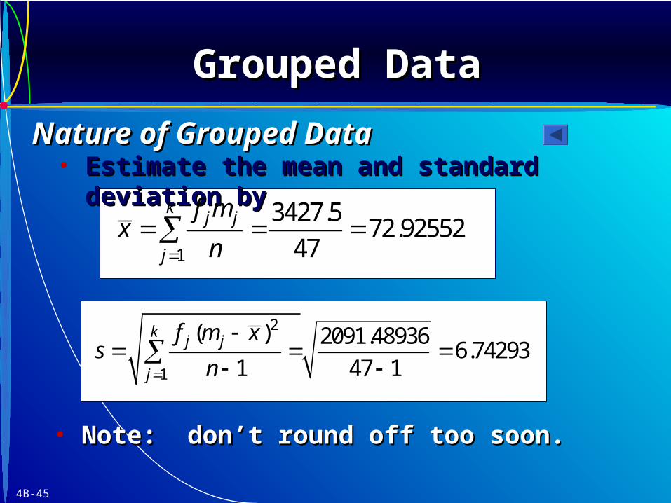
• Estimate the mean and standard deviation byEstimate the mean and standard deviation by

1

3427.572.92552

47

kj j

j

f mx

n

2

1

( ) 2091.489366.74293

1 47 1

kj j

j

f m xs

n

• Note: don’t round off too soon.Note: don’t round off too soon.



4B-46

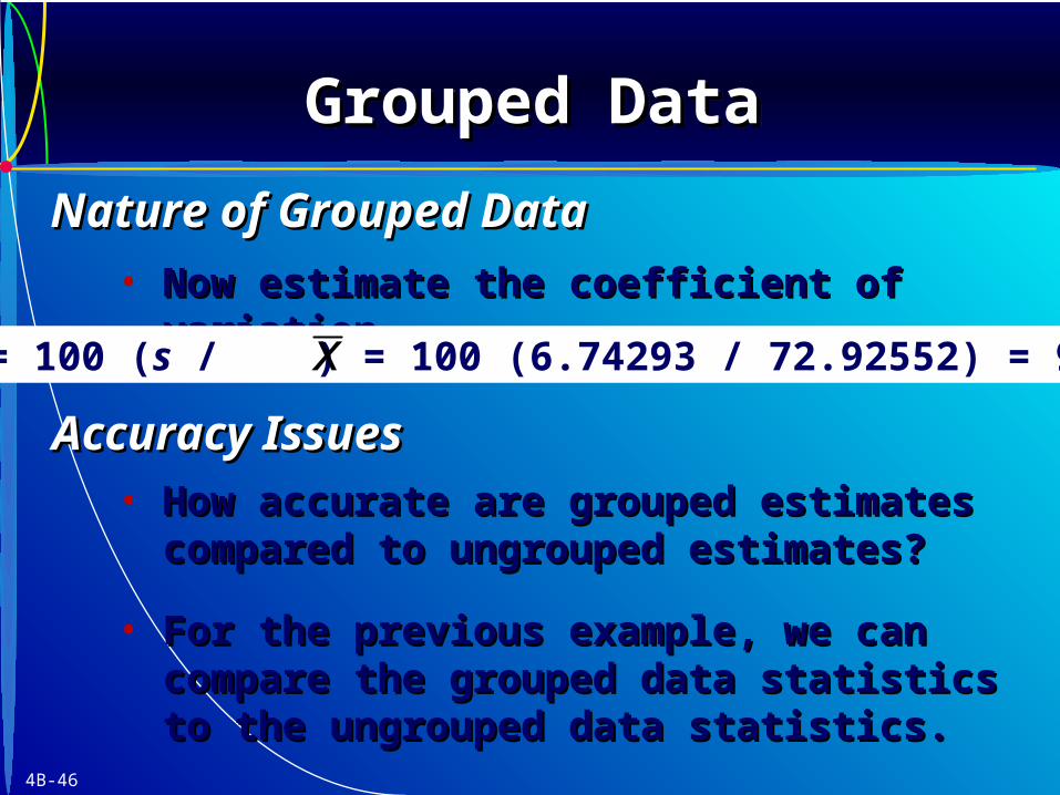
• How accurate are grouped estimates How accurate are grouped estimates compared to ungrouped estimates?compared to ungrouped estimates?

• Now estimate the coefficient of variationNow estimate the coefficient of variation

CV = 100 (s / ) = 100 (6.74293 / 72.92552) = 9.2% x

• For the previous example, we can compare the For the previous example, we can compare the grouped data statistics to the ungrouped data grouped data statistics to the ungrouped data statistics.statistics.



Accuracy IssuesAccuracy Issues

4B-47

• Accuracy tends to improve as the number of bins increases.

• If the first or last class is open-ended, there will be no class midpoint (no mean can be estimated).

• Assume a lower limit of zero for the first class when the data are nonnegative.

• You may be able to assume an upper limit for some variables (e.g., age).

• Median and quartiles may be estimated even with open-ended classes.


Accuracy IssuesAccuracy Issues

4B-48

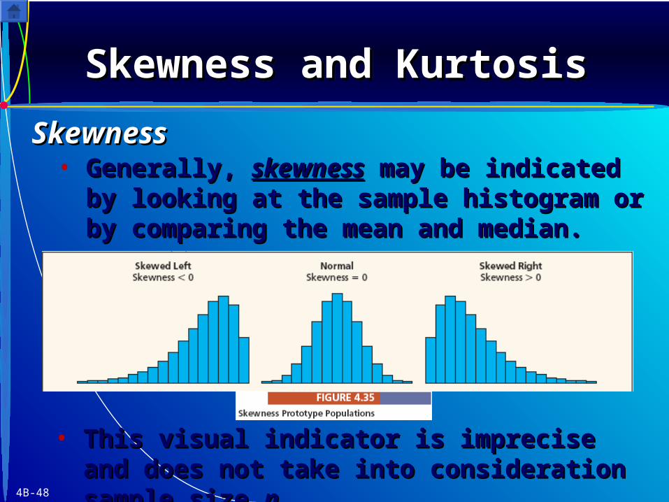
• Generally, Generally, skewnessskewness may be indicated by may be indicated by looking at the sample histogram or by looking at the sample histogram or by comparing the mean and median.comparing the mean and median.

• This visual indicator is imprecise and does not This visual indicator is imprecise and does not take into consideration sample size take into consideration sample size nn..

Skewness and KurtosisSkewness and KurtosisSkewness and KurtosisSkewness and Kurtosis

SkewnessSkewness

4B-49


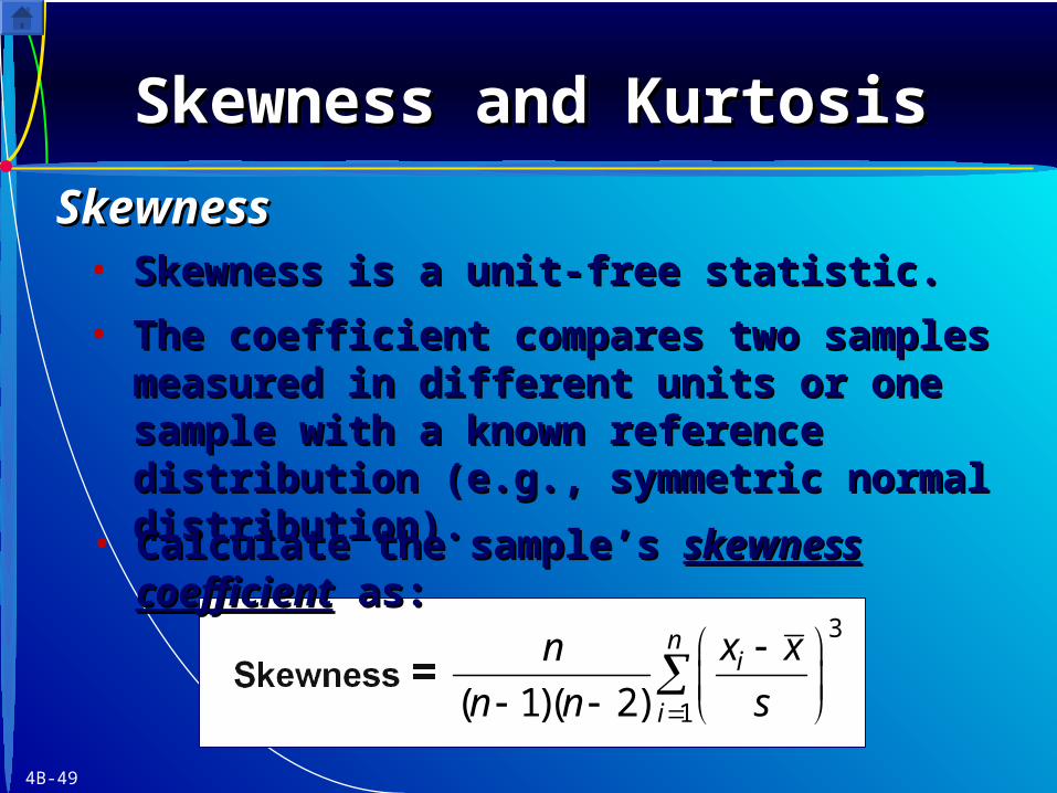
SkewnessSkewness• Skewness is a unit-free statistic. Skewness is a unit-free statistic.

• The coefficient compares two samples The coefficient compares two samples measured in different units or one sample with measured in different units or one sample with a known reference distribution (e.g., a known reference distribution (e.g., symmetric normal distribution).symmetric normal distribution).

• Calculate the sample’s Calculate the sample’s skewness coefficientskewness coefficient as:as:

3

1( 1)( 2)

ni

i

x xn

n n s

4B-50

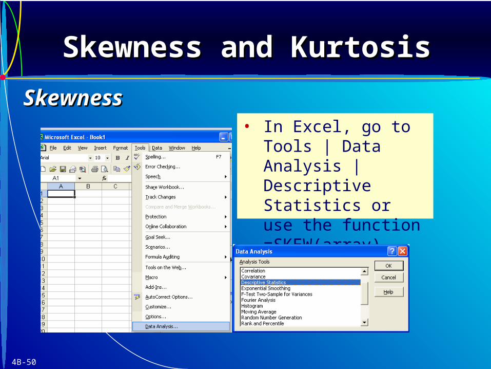
• In Excel, go to Tools | Data Analysis | Descriptive Statistics or use the function =SKEW(array)


SkewnessSkewness

4B-51

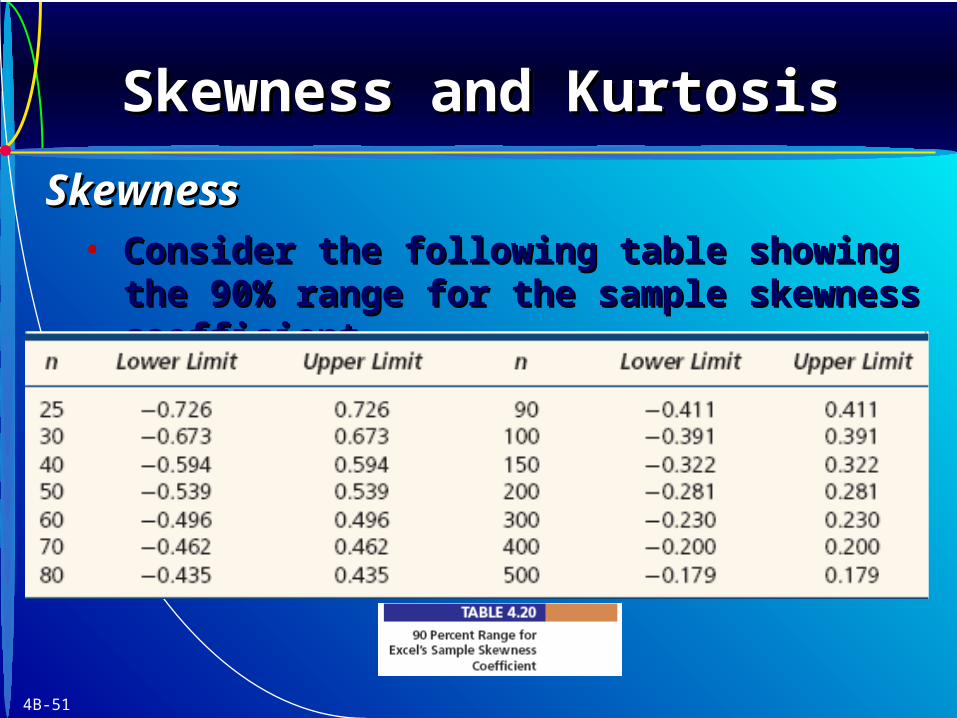
• Consider the following table showing the 90% Consider the following table showing the 90% range for the sample skewness coefficient. range for the sample skewness coefficient.


SkewnessSkewness

4B-52

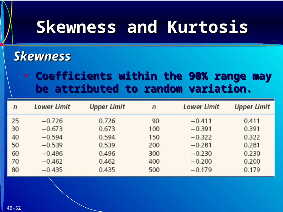
• Coefficients within the 90% range may be Coefficients within the 90% range may be attributed to random variation.attributed to random variation.


SkewnessSkewness

4B-53

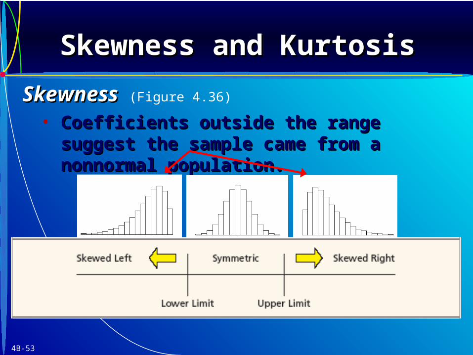
• Coefficients outside the range suggest the Coefficients outside the range suggest the sample came from a nonnormal population.sample came from a nonnormal population.


Skewness Skewness (Figure 4.36)

4B-54

• As As nn increases, the range of chance variation increases, the range of chance variation narrows.narrows.


SkewnessSkewness

4B-55

• KurtosisKurtosis is the relative length of the tails and is the relative length of the tails and the degree of concentration in the center.the degree of concentration in the center.

• Consider three kurtosis prototype shapes.Consider three kurtosis prototype shapes.


KurtosisKurtosis

Heavier tails

4B-56

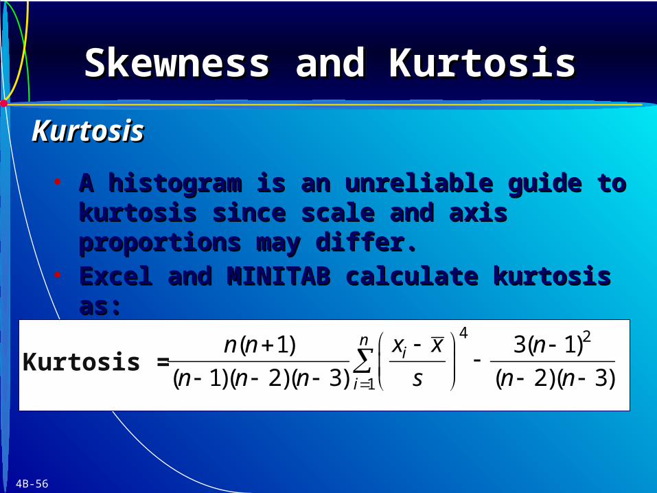
• A histogram is an unreliable guide to kurtosis A histogram is an unreliable guide to kurtosis since scale and axis proportions may differ.since scale and axis proportions may differ.

• Excel and MINITAB calculate kurtosis as:Excel and MINITAB calculate kurtosis as:

Kurtosis = 4 2

1

( 1) 3( 1)

( 1)( 2)( 3) ( 2)( 3)

ni

i

x xn n n

n n n s n n


KurtosisKurtosis

4B-57

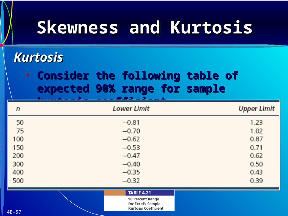
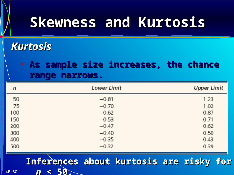
• Consider the following table of expected 90% Consider the following table of expected 90% range for sample kurtosis coefficient.range for sample kurtosis coefficient.


KurtosisKurtosis

4B-58

• A sample coefficient within the ranges may be A sample coefficient within the ranges may be attributed to chance variation.attributed to chance variation.


KurtosisKurtosis

4B-59

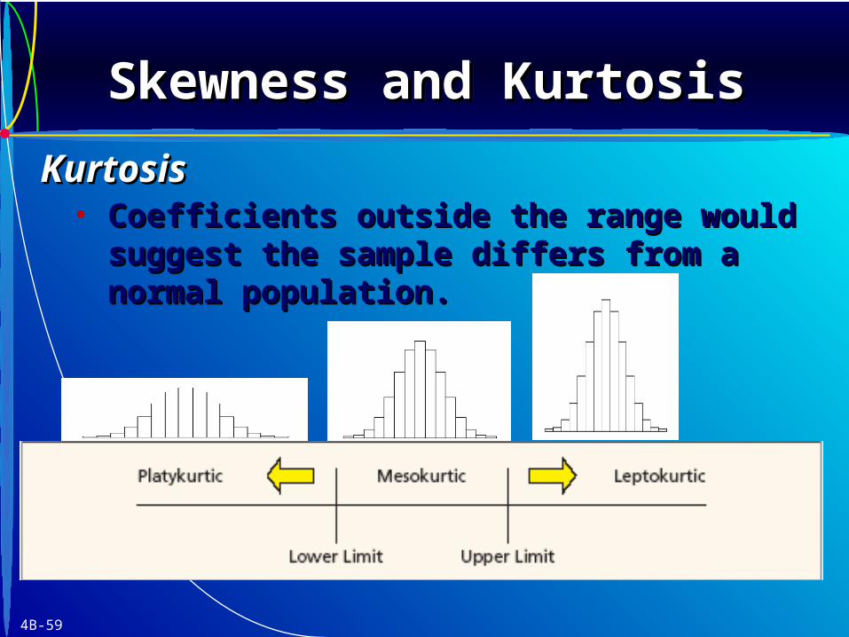
• Coefficients outside the range would suggest Coefficients outside the range would suggest the sample differs from a normal population.the sample differs from a normal population.


KurtosisKurtosis

4B-60

• As sample size increases, the chance range As sample size increases, the chance range narrows. narrows.

Inferences about kurtosis are risky for Inferences about kurtosis are risky for nn < 50. < 50.


KurtosisKurtosis

Applied Statistics in Applied Statistics in Business & EconomicsBusiness & Economics

End of Chapter 4BEnd of Chapter 4B

4B-61

Documents

Descriptive Statistics (Part 2) Chapter44 Standardized Data Percentiles, Quartiles and Box Plots Grouped Data Skewness and Kurtosis McGraw-Hill/Irwin Copyright