Descriptive statistics:Point estimation:

Samplemean and variance

Point estimation

Some Definitions

• The random variables X1, X2,…,Xn are a random sample of size n if:a) The Xi are independent random variables.b) Every Xi has the same probability distribution.

Such X1, X2,…,Xn are also called independent and identically distributed (or i. i. d.) random variables

• A statistic is any function of the observations in a random sample.

• The probability distribution of a statistic is called a sampling distribution.

Sec 7‐2 Sampling Distributions and the Central Limit Theorem 3

Point Estimation• A sample was collected: X1, X2,…, Xn• We suspect that sample was drawn from a 

random variable distribution f(x)• f(x) has k parameters that we do not know• Point estimates are estimates of the parameters of the 

f(x) describing the population based on the  sample– For exponential  PDF: f(x)=λexp(‐λx) one wants to estimate λ– For Bernoulli PDF: px(1‐p)1‐xone wants to estimate p– For normal PDF one wants to estimates both μ and σ

• Point estimates are uncertain: therefore we can talk of averages and standard deviations of point estimates

Sec 7‐1 Point Estimation 4

Point Estimator

Sec 7‐1 Point Estimation 5

1 2

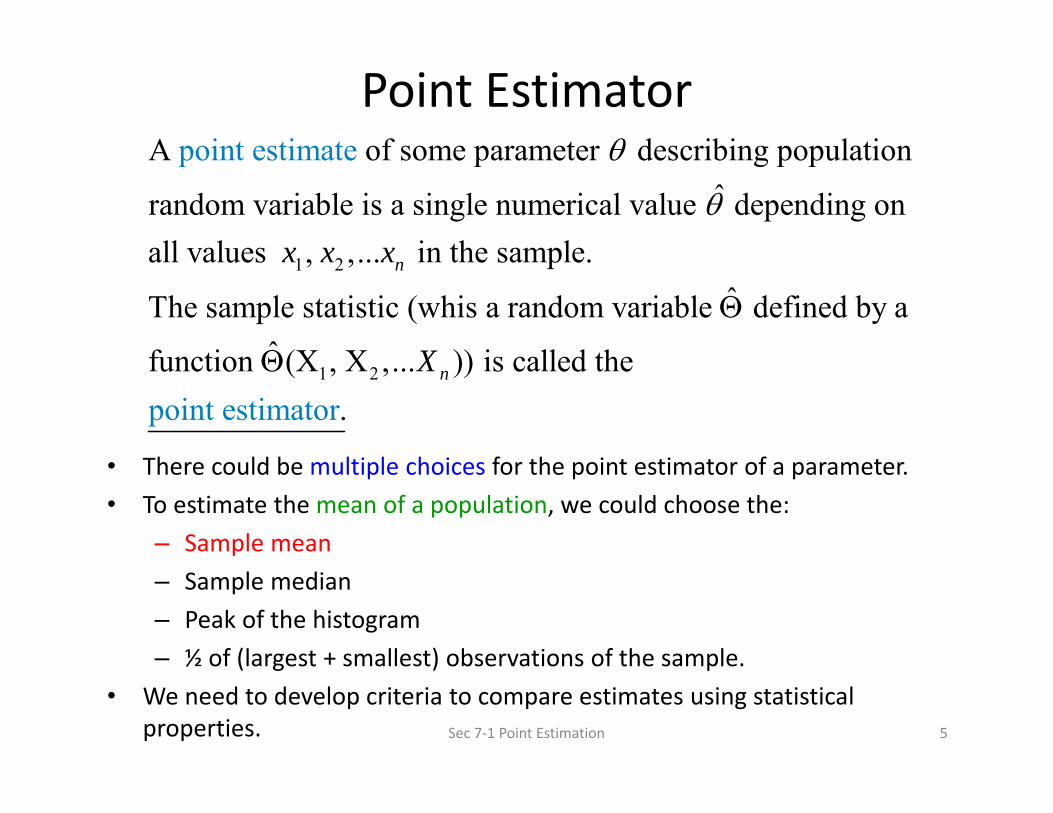
A of some parameter describing population ˆrandom variable is a single numerical value depending on

all values , ,... in the sample.

The sample statistic (whis a random vari

point estimate

nx x x

1 2

ˆable defined by a ˆfunction (X , X ,... )) is called the

.point estimatornX

• There could be multiple choices for the point estimator of a parameter.• To estimate the mean of a population, we could choose the:

– Sample mean– Sample median– Peak of the histogram– ½ of (largest + smallest) observations of the sample.

• We need to develop criteria to compare estimates using statistical properties.

Unbiased Estimators Defined

Sec 7‐3.1 Unbiased Estimators 6

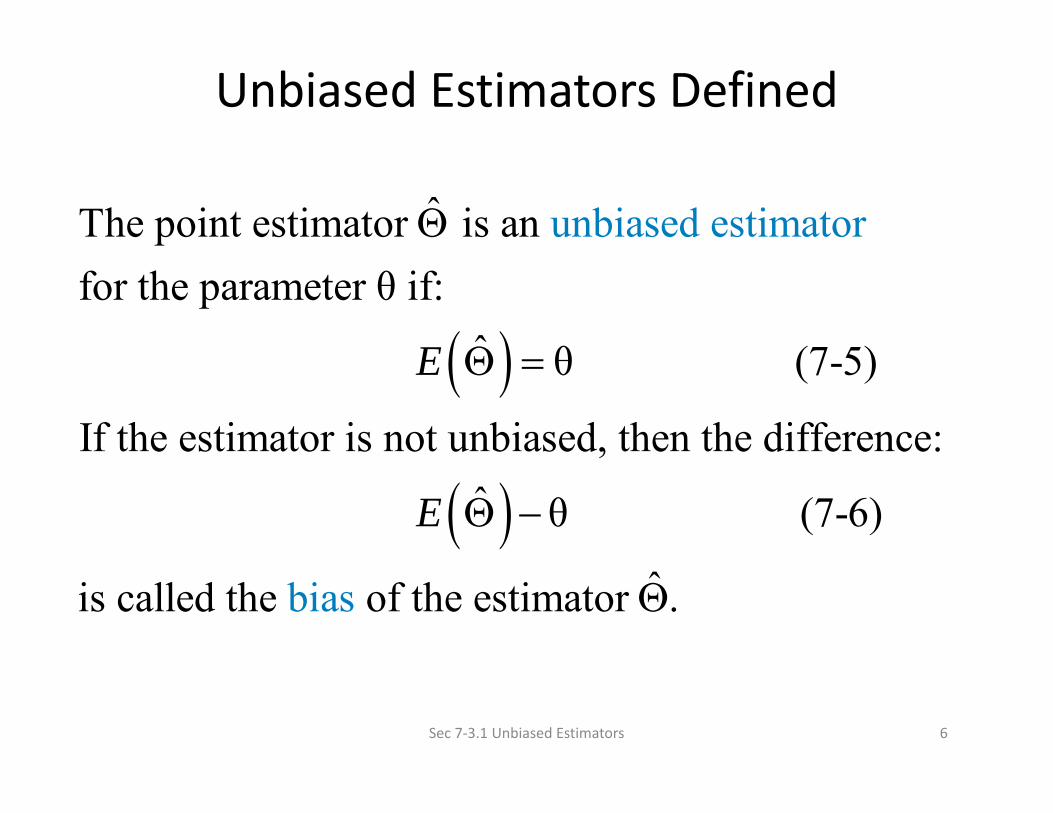
ˆThe point estimator is an for the parameter θ if:

ˆ θ (7-5)

If the estimator is not unbiased, then the difference:

unbiased estimator

E

ˆ θ

.bia

s

(7-6)

ˆis called the of the estimator

E

Mean Squared Error

Conclusion:  The mean squared error (MSE) of the estimator is equal to the variance of the estimator plus the bias squared.  It measures both characteristics.

Sec 7‐3.4 Mean Squared Error of an Estimator 7

2

2 2

The mean squared error of an estimator of the parameter θ is defined as:

ˆ ˆ MSE θ (7-7)

ˆ ˆ ˆCan be rewritten as θ

E

E E E

2ˆ biasV

Methods of Point Estimation

• We will cover two popular methodologies to create point estimates of a population parameter.– Method of moments– Method of maximum likelihood

• Each approach can be used to create estimators with varying degrees of biasedness and relative MSE efficiencies.

Sec 7‐4 Methods of Point Estimation 8

Method of moments for point estimation

What are moments?• A k‐th moment of a random variable is the expected value E(Xk)– First moment: 

– Second moment:  

• A population moment relates to the entire population 

• A sample moment is calculated like its population moments but for a finite sample– Sample first moment = sample mean = 

– Sample k‐th moment 

Sec 7‐4.1 Method of Moments 10

Moment Estimators

Sec 7‐4.1 Method of Moments 11

1 2

1 2

1 2

Let , ,..., be a random sample from either a probability mass function or a probability density function with unknown parameters θ ,θ ,...,θ .

ˆ ˆ ˆThe moment estimators ..., are found by

n

m

m

X X X

m

equating the first population moments

to the first sample moments and solving the resulting simultaneous equations for the unknown parameters.

mm

Exponential Distribution: Moment Estimator‐1st moment 

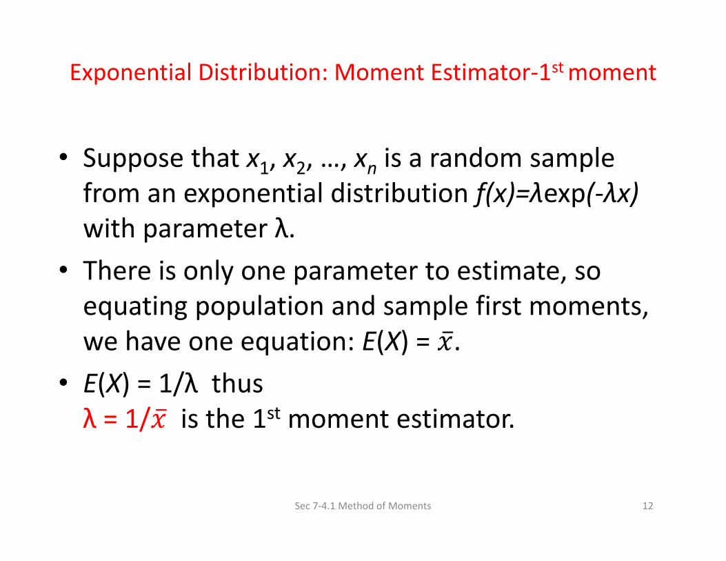
• Suppose that x1, x2, …, xn is a random sample from an exponential distribution f(x)=λexp(‐λx) with parameter λ.

• There is only one parameter to estimate, so equating population and sample first moments, we have one equation: E(X) =  .

• E(X) = 1/λ thus λ = 1/ is the 1st moment estimator.

Sec 7‐4.1 Method of Moments 12

Method of Maximum Likelihood for point estimation

Maximum Likelihood Estimators• Suppose that X is a random variable with probability 

distribution f(x, θ), where θ is a single unknown parameter.  Let x1, x2, …, xn be the observed values in a random sample of size n.  Then the likelihood function of the sample is the probability to get it in a random variable with PDF f(x, θ):

L(θ) = f(x1, θ) ∙ f(x2, θ) ∙…∙ f(xn , θ) (7‐9)

• Note that the likelihood function is now a function of only the unknown parameter θ.  The maximum likelihood estimator (MLE) of θ is the value of θ that maximizes the likelihood function L(θ).

• Usually it is easier to work with logarithms: l(θ) = ln L(θ) 

Sec 7‐4.2 Method of Maximum Likelihood 15

Example 7‐11: Exponential MLE

Let X be a exponential random variable with parameter λ.  The likelihood function of a random sample of size n is:

Sec 7‐4.2 Method of Maximum Likelihood 18

1

1

1

1

1

ln ln

ln0

1 (same as moment estimator)

n

ii i

n xx n

in

ii

n

ii

n

ii

L e e

L n x

d L n xd

n x X

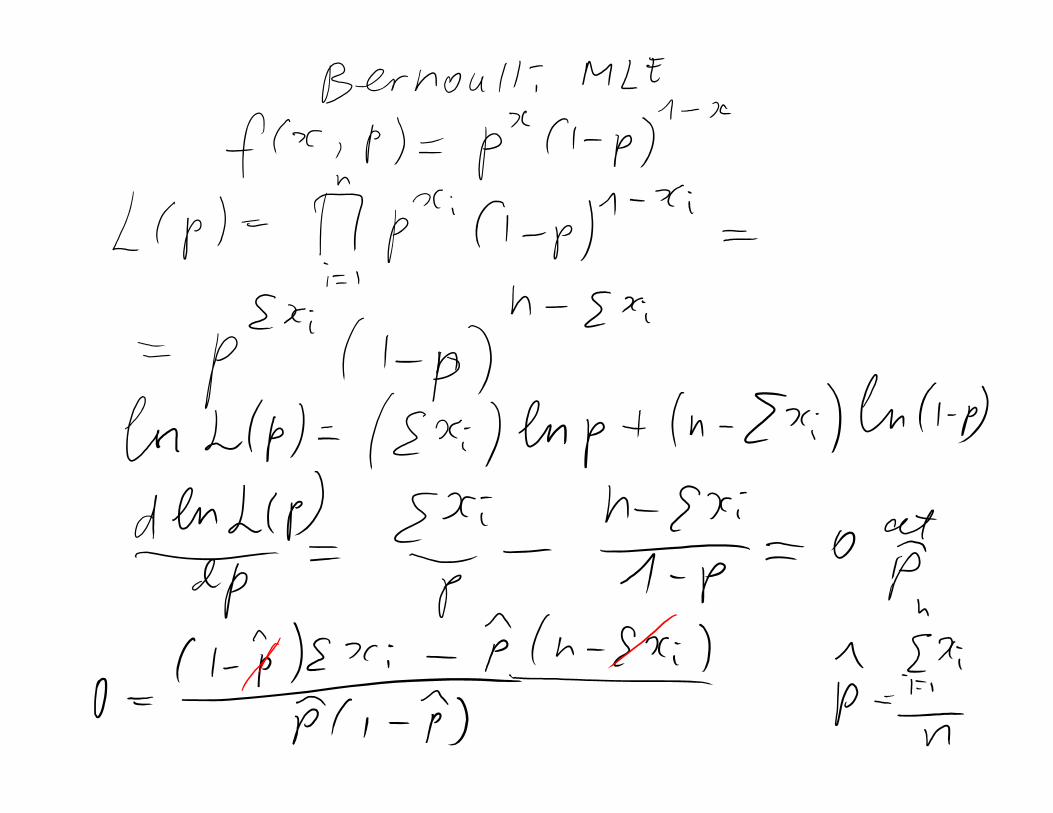
Example 7‐9: Bernoulli MLELet X be a Bernoulli random variable.  The probability mass 

function is f(x;p) = px(1‐p)1‐x, x = 0, 1 where P is the parameter to be estimated.  The likelihood function of a random sample of size n is:

Sec 7‐4.2 Method of Maximum Likelihood 21

1 21 2

11

1 1 1

1

1

1 1

11

1

1 1 ... 1

1 1

ln ln ln 1

ln0

1

nn

nn

ii ii i

i

x x xxx x

n xx n xx

i

n n

i ii i

nn

iiii

n

ii

L p p p p p p p

p p p p

L p x p n x p

n xxd L pdp p p

xp

n

Example 7‐10: Normal MLE for μLet X be a normal random variable with unknown mean μ and 

known variance σ2.  The likelihood function of a random sample of size n is:

Sec 7‐4.2 Method of Maximum Likelihood 24

2 2

22

1

2

1

12

22

222

1

21

1

12

1

2

1ln ln 22 2

ln 1 0

(same as moment estimator)

i

n

ii

n x

i

x

n

n

ii

n

ii

n

ii

L e

e

nL x

d Lx

d

xX

n

MLE for Poisson distribution

26

Credit: XKCD comics 

Matlab exercise

• Generate 100,000 exponentially distributed random numbers with λ=3: f(x)=λexp(‐λx) – Use random('Exponential’…) but read the manual to know how to introduce parameters.

• Get a moment estimate of lambda based on the 1st moment 

• Get a moment estimate of lambda based on the 2nd moment – Second moment of the exponential distribution is E(X2) = E(X)2+Var(X)= 1/λ2 + 1/λ2 = 2/λ2

How I solved it

• Stats=100000; • Y=random('Exponential', 1/3, Stats, 1);%parametrization in MATLAB is 1/lambda• 1/mean(Y) %matching the first moment% ans = 3.0086• sqrt(2/mean(Y.^2)) %matching the second moment

% ans = 3.0081

• Want to make a two‐sided confidence interval of population average μ based on the sample x1, x2,…,xn and its sample mean 

• Assume population standard deviation σ is known• Characterized by: 

– lower‐ and upper‐ confidence limits  L and R– the confidence coefficient 1‐α

• Find L and R such that – Prob(μ>R)=α/2– Prob(μ<L)=α/2– Therefore, Prob(L<μ<R)=1‐α

• For a one‐sided confidence interval, say, upper bound of μ , find R that Prob(μ>R)=α

Two‐sided confidence intervals

Ishikawa et al. (Journal of Bioscience and Bioengineering 2012) studied the force with which bacterial biofilms adhere to a solid surface. 

Five measurements for a bacterial strain of Acinetobactergave readings 2.69, 5.76, 2.67, 1.62, and 4.12 dyne‐cm2. 

Assume that the standard deviation is known  to be 0.66 dyne‐cm2

(a) Find 95% confidence interval for the mean adhesion force

(b) If scientists want the width of the confidence interval to be below 0.55 dyne‐cm2 what number of samples should be? 

Exercise

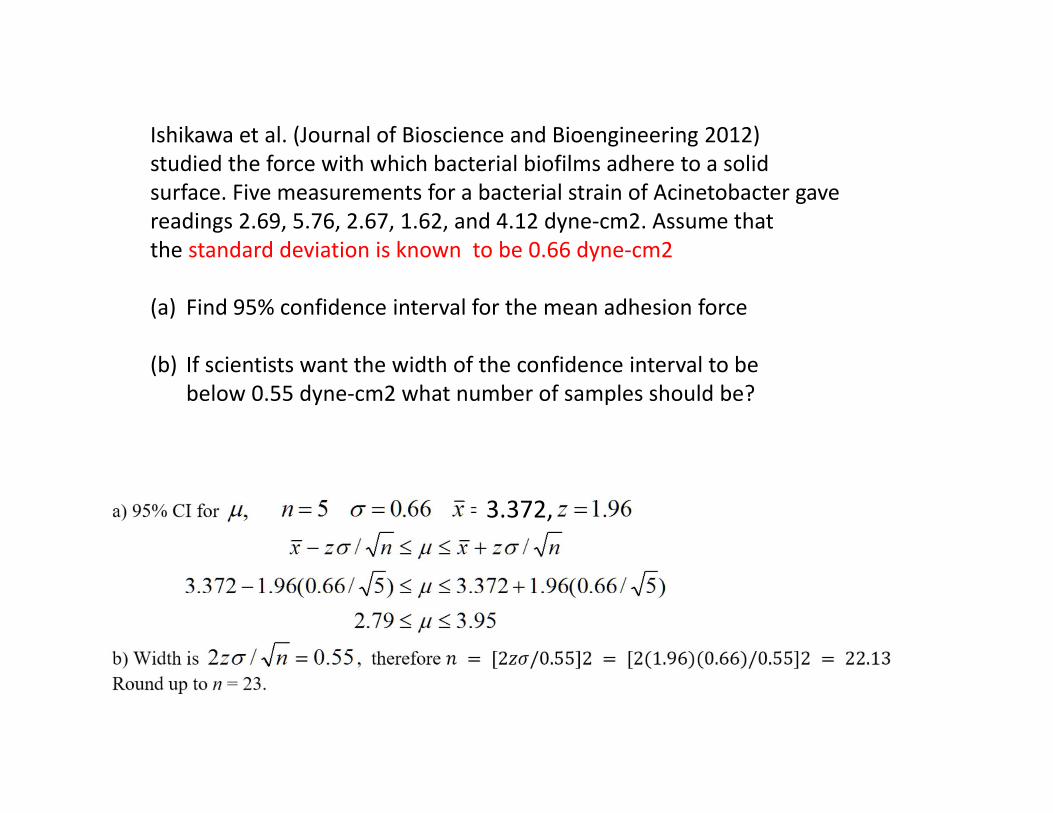
Ishikawa et al. (Journal of Bioscience and Bioengineering 2012) studied the force with which bacterial biofilms adhere to a solid surface. Five measurements for a bacterial strain of Acinetobacter gavereadings 2.69, 5.76, 2.67, 1.62, and 4.12 dyne‐cm2. Assume that the standard deviation is known  to be 0.66 dyne‐cm2

(a) Find 95% confidence interval for the mean adhesion force

(b) If scientists want the width of the confidence interval to be below 0.55 dyne‐cm2 what number of samples should be? 

3.372,

Matlab exercise

• 1000 labs measured average P53 gene expression using n=20 samples drawn from the Gaussian distribution with mu=3; sigma=2;

• Each lab found 95% confidence estimates of the population mean mu based on its sample only

• Count the number of labs, where the population mean lies outside their bounds

• You should get ~50 labs out of 1000 labs