Design & Analysis of Algorithms

Unit 2ADVANCED DATA STRUCTURE

Binary Search Trees• Support many dynamic set operations – SEARCH, MINIMUM, MAXIMUM, PREDECESSOR,

SUCCESSOR, INSERT

• Running time of basic operations on binary search

trees– On average: (lgn)

• The expected height of the tree is lgn

– In the worst case: (n)

• The tree is a linear chain of n nodes

Binary Search Trees• Tree representation:– A linked data structure in which each

node is an object• Node representation:– Key field– Satellite data– Left: pointer to left child– Right: pointer to right child– p: pointer to parent (p [root [T]]

= NIL)• Satisfies the binary-search-tree

property

Left child Right child

L Rparent

key data

Binary Search Tree Example

• Binary search tree property:

– If y is in left subtree of x, then key [y] ≤ key [x]

– If y is in right subtree of x, then key [y] ≥ key [x]

2

3

5

5

7

9

Traversing a Binary Search Tree• Inorder tree walk:– Prints the keys of a binary tree in sorted order– Root is printed between the values of its left and

right subtrees: left, root, right• Preorder tree walk:– root printed first: root, left, right

• Postorder tree walk: left, right, root– root printed last

2

3

5

5

7

9

Preorder: 5 3 2 5 7 9

Inorder: 2 3 5 5 7 9

Postorder: 2 5 3 9 7 5

Traversing a Binary Search TreeAlg: INORDER-TREE-WALK(x)1. if x NIL2. then INORDER-TREE-WALK ( left [x] )3. print key [x]4. INORDER-TREE-WALK ( right [x] )

• E.g.:

• Running time: – (n), where n is the size of the tree rooted at x

2

3

5

5

7

9

Output: 2 3 5 5 7 9

Binary Search Trees - Summary• Operations on binary search trees:– SEARCH O(h)

– PREDECESSOR O(h)

– SUCCESOR O(h)

– MINIMUM O(h)

– MAXIMUM O(h)

– INSERT O(h)

– DELETE O(h)

• These operations are fast if the height of the tree is small – otherwise their performance is similar to that of a linked list

Red-Black Trees

• “Balanced” binary trees guarantee an O(lgn) running time on the basic dynamic-set operations

• Red-black-tree– Binary tree with an additional attribute for its nodes:

color which can be red or black– Constrains the way nodes can be colored on any path

from the root to a leaf• Ensures that no path is more than twice as long as another

the tree is balanced

– The nodes inherit all the other attributes from the binary-search trees: key, left, right, p

Red-Black-Trees Properties

1. Every node is either red or black

2. The root is black

3. Every leaf (NIL) is black

4. If a node is red, then both its children are black• No two red nodes in a row on a simple path from the root

to a leaf

5. For each node, all paths from the node to descendant leaves contain the same number of black nodes

Example: RED-BLACK-TREE

• For convenience we use a sentinel NIL[T] to represent all the NIL nodes at the leafs– NIL[T] has the same fields as an ordinary node– Color[NIL[T]] = BLACK– The other fields may be set to arbitrary values

26

17 41

30 47

38 50

NIL NIL

NIL

NIL NIL NIL NIL

NIL

Black-Height of a Node

• Height of a node: the number of edges in a longest path to a leaf

• Black-height of a node x: bh(x) is the number of black nodes (including NIL) on the path from x to leaf, not counting x

26

17 41

30 47

38 50

NIL NIL

NIL

NIL NIL NIL NIL

NIL

h = 4bh = 2

h = 3bh = 2

h = 2bh = 1

h = 1bh = 1

h = 1bh = 1

h = 2bh = 1 h = 1

bh = 1

Properties of Red-Black-Trees• Claim– Any node with height h has black-height ≥ h/2

• Proof– By property 4, at most h/2 red nodes on the path

from the node to a leaf– Hence at least h/2 are black 26

17 41

30 47

38 50

Property 4: if a node is red then both its children are black

Operations on Red-Black-Trees• The non-modifying binary-search-tree operations

MINIMUM, MAXIMUM, SUCCESSOR,

PREDECESSOR, and SEARCH run in O(h) time

– They take O(lgn) time on red-black trees

• What about TREE-INSERT and TREE-DELETE?

– They will still run on O(lgn)

– We have to guarantee that the modified tree will still be

a red-black tree

Rotations• Operations for restructuring the tree after insert

and delete operations on red-black trees

• Rotations take a red-black-tree and a node within the tree and:– Together with some node re-coloring they help restore

the red-black-tree property

– Change some of the pointer structure

– Do not change the binary-search tree property

• Two types of rotations:– Left & right rotations

Left Rotations• Assumptions for a left rotation on a node x:– The right child of x (y) is not NIL– Root’s parent is NIL

• Idea:– Pivots around the link from x to y– Makes y the new root of the subtree– x becomes y’s left child– y’s left child becomes x’s right child

LEFT-ROTATE(T, x)1. y ← right[x] Set y►

2. right[x] ← left[y] ► y’s left subtree becomes x’s right subtree

3. if left[y] NIL4. then p[left[y]] ← x ► Set the parent relation from left[y] to x

5. p[y] ← p[x] ► The parent of x becomes the parent of y

6. if p[x] = NIL7. then root[T] ← y8. else if x = left[p[x]]9. then left[p[x]] ← y10. else right[p[x]] ← y11.left[y] ← x ► Put x on y’s left

12.p[x] ← y ► y becomes x’s parent

Example: LEFT-ROTATE

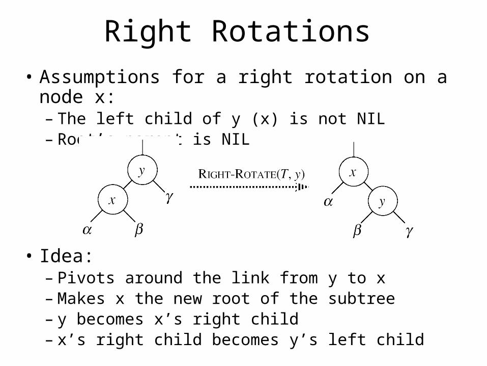
Right Rotations• Assumptions for a right rotation on a node x:– The left child of y (x) is not NIL– Root’s parent is NIL

• Idea:– Pivots around the link from y to x– Makes x the new root of the subtree– y becomes x’s right child– x’s right child becomes y’s left child

Insertion

• Goal:

– Insert a new node z into a red-black-tree

• Idea:

– Insert node z into the tree as for an ordinary binary search

tree

– Color the node red

– Restore the red-black-tree properties

• Use an auxiliary procedure RB-INSERT-FIXUP

RB-INSERT(T, z)

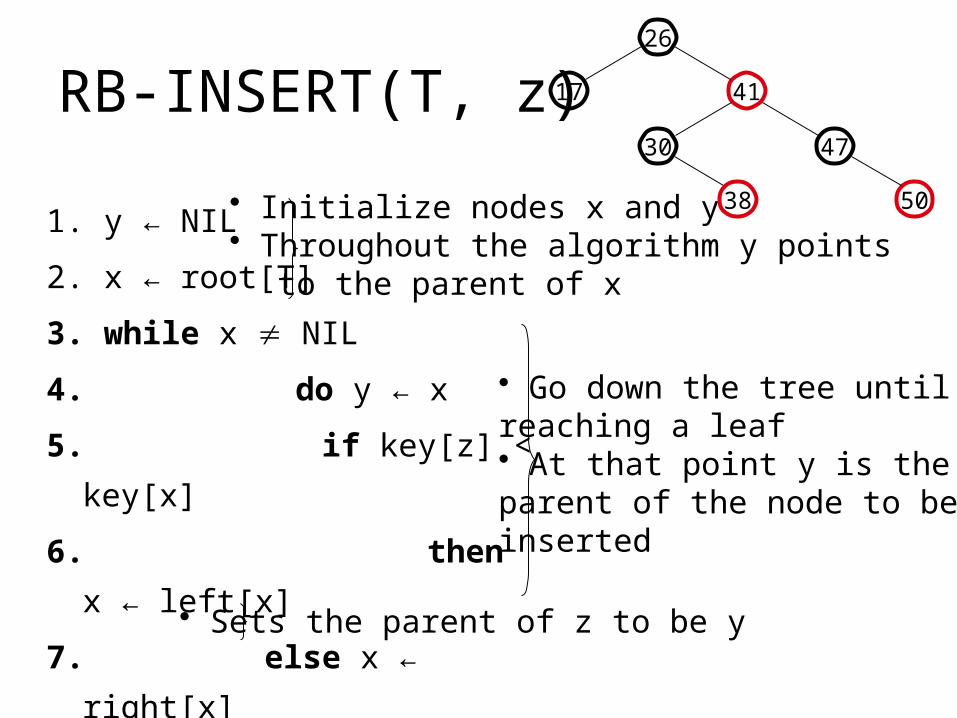
1. y ← NIL

2. x ← root[T]

3. while x NIL

4. do y ← x

5. if key[z] < key[x]

6. then x ← left[x]

7. else x ← right[x]

8. p[z] ← y

• Initialize nodes x and y• Throughout the algorithm y points

to the parent of x

• Go down the tree untilreaching a leaf• At that point y is theparent of the node to beinserted

• Sets the parent of z to be y

26

17 41

30 47

38 50

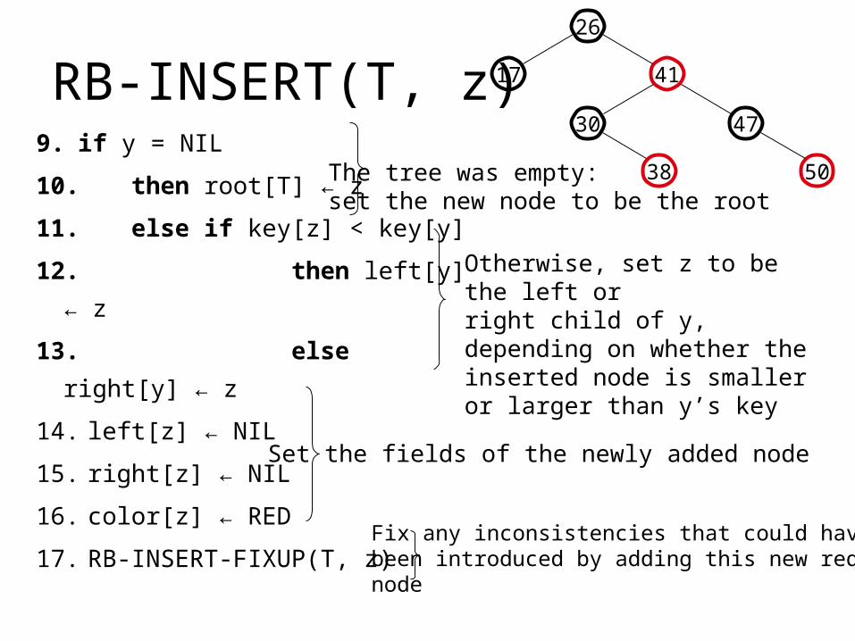
RB-INSERT(T, z)9. if y = NIL

10. then root[T] ← z

11. else if key[z] < key[y]

12. then left[y] ← z

13. else right[y] ← z

14. left[z] ← NIL

15. right[z] ← NIL

16. color[z] ← RED

17. RB-INSERT-FIXUP(T, z)

The tree was empty: set the new node to be the root

Otherwise, set z to be the left orright child of y, depending on whether the inserted node is smaller or larger than y’s key

Set the fields of the newly added node

Fix any inconsistencies that could havebeen introduced by adding this new rednode

26

17 41

30 47

38 50

RB Properties Affected by Insert1. Every node is either red or black

2. The root is black

3. Every leaf (NIL) is black

4. If a node is red, then both its children are black

5. For each node, all paths

from the node to descendant

leaves contain the same number

of black nodes

OK!

If z is the root not OK

OK!

26

17 41

4738

50

If p(z) is red not OKz and p(z) are both red

OK!

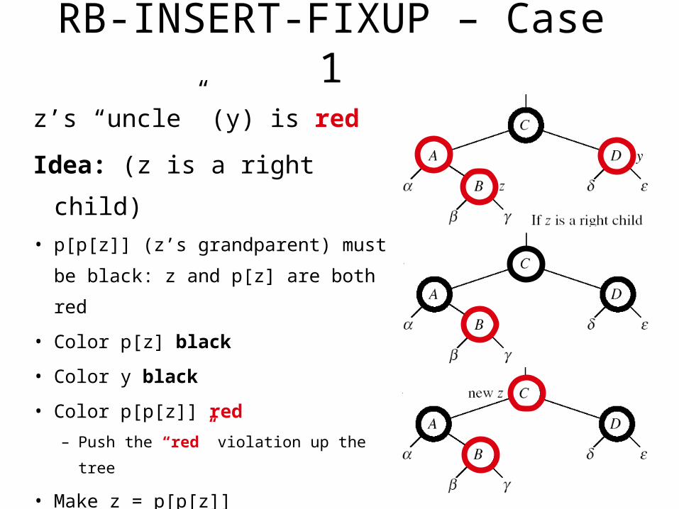
RB-INSERT-FIXUP – Case 1

z’s “uncle” (y) is red

Idea: (z is a right child)• p[p[z]] (z’s grandparent) must be

black: z and p[z] are both red

• Color p[z] black

• Color y black

• Color p[p[z]] red

– Push the “red” violation up the tree

• Make z = p[p[z]]

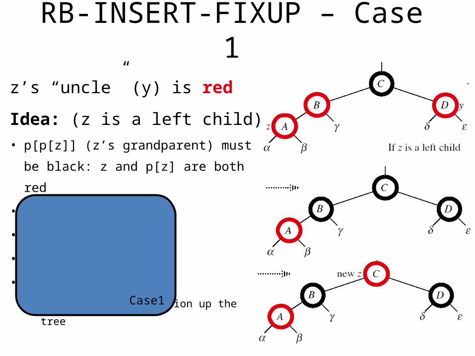
RB-INSERT-FIXUP – Case 1

z’s “uncle” (y) is red

Idea: (z is a left child)• p[p[z]] (z’s grandparent) must be

black: z and p[z] are both red

• color[p[z]] black

• color[y] black

• color p[p[z]] red

• z = p[p[z]]

– Push the “red” violation up the tree

Case1

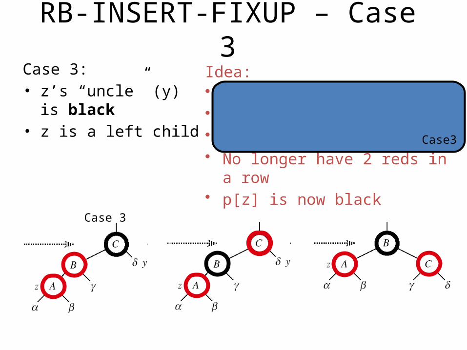
RB-INSERT-FIXUP – Case 3Case 3: • z’s “uncle” (y) is black• z is a left child

Case 3

Idea:• color[p[z]] black • color[p[p[z]]] red• RIGHT-ROTATE(T, p[p[z]])• No longer have 2 reds in a row• p[z] is now black

Case3

RB-INSERT-FIXUP – Case 2Case 2: • z’s “uncle” (y) is black• z is a right childIdea:• z p[z]• LEFT-ROTATE(T, z) now z is a left child, and both z and p[z] are red case 3

Case 2 Case 3

Case2

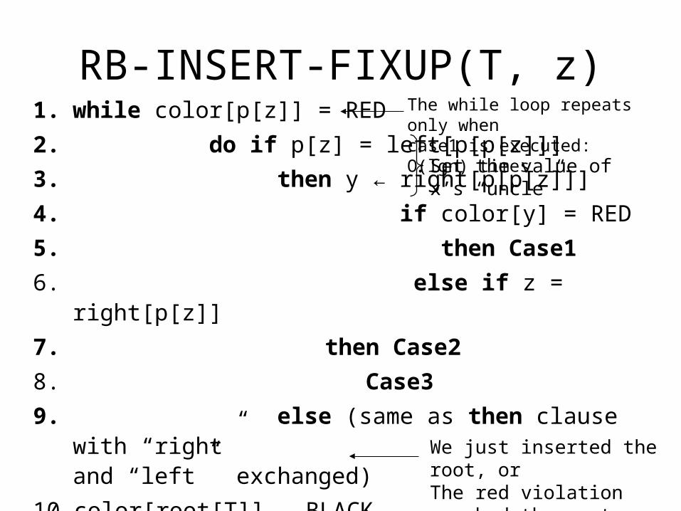
RB-INSERT-FIXUP(T, z)1. while color[p[z]] = RED

2. do if p[z] = left[p[p[z]]]

3. then y ← right[p[p[z]]]

4. if color[y] = RED

5. then Case16. else if z = right[p[z]]

7. then Case28. Case39. else (same as then clause with “right”

and “left” exchanged)10. color[root[T]] ← BLACK

The while loop repeats only whencase1 is executed: O(lgn) times

Set the value of x’s “uncle”

We just inserted the root, orThe red violation reached the root

Example

11Insert 4

2 14

1 157

85

4

y

11

2 14

1 157

85

4

z

Case 1

y

z and p[z] are both redz’s uncle y is redz

z and p[z] are both redz’s uncle y is blackz is a right child

Case 2

11

2

14

1

15

7

8

5

4

z

y Case 3

z and p[z] are redz’s uncle y is blackz is a left child

112

141

15

7

85

4

z

Analysis of RB-INSERT

• Inserting the new element into the tree O(lgn)

• RB-INSERT-FIXUP

– The while loop repeats only if CASE 1 is executed

– The number of times the while loop can be executed is

O(lgn)

• Total running time of RB-INSERT: O(lgn)

Red-Black Trees - Summary

• Operations on red-black-trees:– SEARCH O(h)

– PREDECESSOR O(h)

– SUCCESOR O(h)

– MINIMUM O(h)

– MAXIMUM O(h)

– INSERT O(h)

– DELETE O(h)

• Red-black-trees guarantee that the height of the tree will be O(lgn)