1

Design and Analysis of a Blind Juggling RobotPhilipp Reist, Graduate Student Member, IEEE, and Raffaello D’Andrea, Fellow, IEEE

Abstract—We present the design of the Blind Juggler, a robotthat is able to juggle an unconstrained ball without feedbackat heights of up to 2 meters. The robot actuates a parabolicaluminum paddle with a linear motor. We achieve open-loopstability of the ball trajectory with two design parameters: 1) thecurvature of the parabolic paddle and 2) the acceleration of thepaddle at impact. We derive a linear map of perturbations ofthe nominal ball trajectory over a single bounce, and obtainlocal stability of the trajectory by tuning the eigenvalues of thismapping with the two design parameters. We consider 9 ballstates in this analysis, including ball spin. Experimental dataprovides the impact states of the ball and paddle. From this data,we can identify system parameters and infer the process noiseintroduced into the system. We then combine the experimentalnoise power spectral densities with a model of the system andoptimize the design parameters such that the impact of theprocess noise on juggling performance is minimized. Theoreticalas well as experimental results of the optimization are discussed.

Index Terms—Dynamics, Dexterous Manipulation, MechanismDesign, Bouncing Ball, Juggling.

I. INTRODUCTION

THE Blind Juggler, shown in Fig. 1, demonstrates thathigh-performance robotic juggling of unconstrained balls

is possible without using sensors. The Blind Juggler can juggleat apex heights of up to 2 m, even though the robot cannot tiltor pan the aluminum paddle, which is actuated by a linearmotor. In effect, the Blind Juggler can stabilize a ball in threedimensions with only a single actuated degree of freedom.Since there is no feedback, we achieve open-loop stabilityof the ball trajectory using two key design elements: 1) Thepaddle has a slightly concave, parabolic shape, which keepsthe ball from bouncing off the robot; 2) A decelerating strikingmotion of the paddle stabilizes the apex height of the ball. Inexperiments, the Blind Juggler is able to continuously jugglea variety of balls at different heights, and exhibits substantialrobustness to horizontal and vertical perturbations.

In particular, the two key design parameters are the cur-vature of the parabolic paddle shape and the acceleration ofthe paddle at ball impact. We determine the specific valuesof the design parameters by analyzing the local stabilityof the nominal ball trajectory. Using a model of the balldynamics, we perform a perturbation analysis of the trajectoryand calculate how perturbations introduced at the apex map tothe next apex. We consider nine ball states in this analysis:all translational positions and velocities, and ball spin. Usingfirst-order approximations to the system dynamics, we obtain alinear map, i.e. a linearized Poincare map of the perturbations

P. Reist and R. D’Andrea are with the Institute for Dynamic Systems andControl at ETH Zurich, Switzerland (e-mail: reistp, rdandrea@ethz.ch).Additional information about the robot, including many videos, may be foundat www.blindjuggler.org.

Fig. 1. The Blind Juggler bouncing a superball. The user interface featurestwo buttons to control the juggling height.

over a single bounce. We tune the eigenvalues of this mappingwith the paddle curvature and acceleration to achieve localstability for a range of apex heights and ball parameters.

We use a video camera and a microphone to measureimpact states of the ball and paddle in order to assess jugglingperformance in terms of impact location and apex heightvariance. We also use these measurements to identify systemparameters such as the ball coefficient of restitution and toinfer the process noise introduced into the system by imperfectpaddle motions and stochastic ball impact properties.

We use the process noise measurements to refine the designparameters and improve juggling performance. First, we set upa linear, time-invariant system that models how the noise inputmaps to the outputs: the deviations in ball impact locationand apex height. These outputs are what we want to keepsmall. Next, we use the frequency response of the linearsystem together with the experimental power spectral densitiesof the process noise to calculate the output variance as afunction of the design parameters. We then find the designparameters that minimize the output variance. Theoreticalresults predict a performance improvement for the apex height

2

and no improvement for the impact location. This is alsoconfirmed in experiments. The small impact of the paddlecurvature on the impact location variance allows us to choosethe curvature according to secondary criteria such as, forexample, maximal achievable apex height.

This paper is structured as follows: After an overview of re-lated work, we derive the nominal ball trajectory in Section II.The perturbation analysis is presented in Section III. We findstabilizing design parameters in Section IV. The prototypeof the Blind Juggler and experimental results are discussedin Section V. Lastly, we optimize the design parameters anddiscuss theoretical and experimental results in Section VI.

A. Related Work

This paper is based on previous work published in [1],where we presented preliminary results obtained with a pro-totype of the Blind Juggler. New contributions comparedto previous work include the stability analysis for 9 ballstates (previously a planar model) and using measured noisepower spectral densities for the design parameter optimization(previously assumed white process noise).

The bouncing ball system has received attention in dynam-ics, as it is a simple system that exhibits rich dynamical behav-ior, i.e. period doubling (bifurcations) leading to chaos [2], [3].Holmes showed that even with energy dissipation present inthe form of a coefficient of restitution, chaotic motions of theball result for sufficiently high excitation levels [2]. Vincentpresented a control strategy for bouncing a ball at a fixedheight that exploits chaotic behavior in [4].

In robotics, juggling is considered a challenging dexteroustask. Buhler et al. were amongst the first to study roboticjuggling using a planar juggling robot [5]. The robot consistsof a rotating bar equipped with a billiard cushion battinga puck on an inclined table. Using position feedback, therobot is able to simultaneously juggle up to two pucks. Ituses a feedback strategy called the mirror law introduced byBuhler et al. [6], [7]. The algorithm defines the trajectory ofthe paddle as a mirrored (about the desired impact height)and scaled version of the ball’s trajectory. Consequently, thisrequires constant tracking of the ball’s position. The mirror lawproduces paddle trajectories that accelerate at impact, whichcontrasts with the results presented in this paper, and withresults obtained by Schaal et al., who analyzed the apex heightstabilizing property of a decelerating paddle for an open-loopbouncing ball system [8]. An interesting aside is that Schaalet al. found that a decelerating striking motion is a strategyintuitively used by humans when trying to bounce a ball ata fixed height on a racket [9]. The related task of dribblinga basketball with a robot arm using force or vision feedbackwas explored by Batz et al. [10]. In legged robotics, a hoppingrobot is similar to a bouncing ball system. Ringrose presentedthe design of a self-stabilizing monopod featuring a curvedfoot in [11], which is similar to sensorless bouncing of a ballon a parabolic paddle.

Robotic juggling has motivated the development of ad-vanced control methods such as Burridge’s work on jugglingan unconstrained ball in the presence of obstacles using a

cascade of controllers [12]. This control strategy, which usesvision feedback, was evaluated on a direct drive robot arm,the Buhgler. With the same arm, Rizzi et al. extended themirror law to unconstrained balls and achieved simultaneousjuggling of two balls [13]. Kulchenko et al. developed a modelpredictive control strategy for juggling up to two unconstrainedtable tennis balls with a single racket using a haptic robot [14].Other work on control involving juggling robots includesSanfelice’s hybrid control strategies to stabilize juggling ofmultiple balls [15], and Zavala-Rıo’s method to deal withuncertainty in the coefficient of restitution [16]. Schaal et al.used a juggling setup to develop robot learning strategies,where a robot arm iteratively learns to juggle a ball on aplate [17]. Sakaguchi et al. also studied learning strategiesusing a planar robot arm that juggles bean bags by throwingand catching [18].

Related to the concepts presented here is the work byRonsse et al., who analyzed different juggling systems [19]–[22], and introduced the term “blind” juggling robot in [22],where they presented a planar ball-in-wedge juggling robotthat is able to juggle purely feed-forward or with feedbackusing measured impact times. Their robot is even able togenerate a juggling pattern similar to the shower pattern,where the balls follow a circular path. In [21], [22], Ronsseaddressed robustness of the bouncing ball system to staticand dynamic errors in the ball’s coefficient of restitution. Theauthors first derived the transfer function of the errors to thepost-impact velocity perturbations. Then, they placed the zeroof the transfer function by adjusting the paddle accelerationto either compensate for static or dynamic errors. This is analternative strategy to the parameter optimization we presentin this paper. Hobbelen et al. presented an H2-norm inspiredgait sensitivity norm that can be used to determine disturbancerejection capabilities of limit cycle walking robots [23]. Theauthors further showed that a stability measure, such as thespectral radius of a linearized Poincare map, is a poor indicatorof actual system performance in the presence of stochastic dis-turbances. They proposed their H2-norm inspired performancemetric as a better indicator. The gait sensitivity norm [24]can serve as a guide for design parameter selection for awalking robot, which is similar to the variance optimizationwe present in this paper. Mombaur et al. used optimizationto find stabilizing design parameters for open-loop walkingrobots in [25]. The authors used the spectral radius of thelinearized Poincare map as the objective function to minimizein order to find design parameters resulting in a spectral radiussmaller than one, which implies stability.

The Blind Juggler is able to juggle unconstrained ballswithout sensing. In the literature, many robots are studiedthat juggle constrained balls. Examples include the singledegree of freedom bouncing ball setup by Vincent [4], or theplanar juggling robots analyzed by Buhler [5] and Ronsse [22].Robots juggling unconstrained balls in three dimensions typ-ically feature a robotic arm; the robot used by Rizzi et al.in [13] is one such example. These more complex robotsuse cameras to continuously track the ball’s position. Schaalet al. presented an open-loop juggling robot that features apaddle that passively keeps the ball in its center: they used

3

0 1 2− 2+ 3 4

Fig. 2. Sketch of nominal ball trajectory. The ball starts at rest at the apex, 0.It is then subject to free fall, 1, before it impacts with the paddle, 2−. Afterimpact 2+, the ball is again subject to free fall, 3, until it reaches again theapex, 4, which is identical to the initial apex, 0.

a trampoline-like racket to stabilize the horizontal degrees offreedom of the ball [8]. Their focus, however, was on theanalysis of the vertical stability of the ball.

II. NOMINAL BALL TRAJECTORY

We introduce the nominal ball trajectory, which is sketchedin Fig. 2. In the stability analysis, we consider the ballstate S := (x, x, ωy, y, y, ωx, z, z, ωz)

T, where T denotes thetranspose. All elements are defined in the coordinate system Jshown in Fig. 3. The positions x, y, z describe the locationof the center of the ball. The ball velocities are x, y, z, andthe ball spins ωx, ωy, ωz are defined by the right-hand rule.We choose the particular grouping of the states since the spinωy interacts with the horizontal velocity x at impact, and ωxwith y.

Nominally, all states except z, z are zero. However, becausewe use the full nominal ball states in the perturbation analysisin the next section, we derive them in the following.

A. Initial Apex

The ball starts at time t = 0 at the nominal apex heightz(0) = H . Its state is

S0 = (0, 0, 0, 0, 0, 0, H, 0, 0)T (1)

where the subscript 0 denotes the initial apex and an overbardenotes a nominal state.

B. Free Fall

Next, the ball is in free fall. We ignore aerodynamic dragand obtain the differential equation

z(t) = −g (2)

where g = 9.81 m/s2 is the gravitational acceleration. Giveninitial conditions z0, z0 at t = 0, its solution is

z(t) = −g2t2 + z0t+ z0 (3)

z(t) = −gt+ z0. (4)

Jz

JyJx

g

Fig. 3. Definition of the coordinate system J. The sketched ball and paddleare at nominal impact positions. The origin of J is fixed at the center of theball at nominal impact position, and the z-axis is aligned with gravity g.

The nominal initial conditions are ˙z0 = 0, z0 = H . The freefall ends at impact with the paddle, which is at z(T ) = 0,see Fig. 3. The nominal impact time is

T =

√2H

g(5)

and the nominal ball impact velocity is

˙z1 = −gT. (6)

The ball state at t = T is denoted with the subscript 1. Thenominal state is

S1 = (0, 0, 0, 0, 0, 0, 0, ˙z1, 0)T. (7)

Nominally, S1 and the pre-impact (−) ball state are identicalS−2 = S1. We still introduce two separate nominal states sincein the perturbation analysis, the perturbed states at the nominalimpact time and at the actual impact time differ.

C. ImpactNominally, the vertical ball velocity is inverted at impact

such that the initial apex height is reached again. The post-impact (+) ball state is therefore

S+2 = (0, 0, 0, 0, 0, 0, 0,− ˙z1, 0)

T. (8)

We further derive the nominal paddle state at impact. Thepaddle state is P = (zP, zP) T, since the paddle has only asingle translational degree of freedom. The state is defined inthe coordinate system J, and zP captures the height of thecenter of the paddle surface. At impact, the ball is in contactwith the paddle (see Fig. 3), and the nominal paddle state istherefore

P2 = P1 = (−R, ˙zP1)T (9)

where R is the ball radius and the nominal paddle velocity˙zP1 is obtained using Newton’s impact law:

z+ = −ez z− + (1 + ez)zP (10)

where z−, z+ are the pre- and post-impact ball velocities,respectively. Damping losses at impact are modeled by thevertical coefficient of restitution ez ∈ [0, 1]. In (10), we assumethat the ratio of the ball mass to the paddle mass is smallenough for the change in paddle impulse to be negligible (thisratio is ≈ 3×10−4 for the Blind Juggler). For this reason, wedo not distinguish between the pre- and post-impact paddlestate and omit the superscripts (+,−). With (7) and (8) in(10), we find

˙zP1 = − ˙z11− ez1 + ez

. (11)

4

D. Free Fall after Impact and Apex

After impact, the ball is in free fall until it reaches thenominal apex height again. The duration of the second freefall is identical to the first, resulting in the final apex timet = 2T . Nominally, the state after free fall (subscript 3), thestate at final apex time (subscript 4), and the initial apex stateare all identical

S3 = S4 = S0. (12)

We introduce S3 because, in the perturbation analysis, theperturbed ball states after free fall and at nominal apex timeare not identical.

III. PERTURBATION ANALYSIS

In the following, we derive how perturbations, added to thenominal ball apex state, map over a single bounce to the nextapex, i.e. from 0 to 4 in Fig. 2. We assume that the pertur-bations are small and use first-order approximations to thesystem dynamics. Experimental data presented in Section Vshows that the perturbations are indeed small. Therefore, theactual nonlinear system dynamics are captured well by a first-order model. In the following analysis, we derive the matricesthat describe the first-order perturbation dynamics of each partof the trajectory illustrated in Fig. 2. These matrices form thebasis for the results presented in the rest of this paper. Thematrices show that to first order, the ball perturbation dynamicsin x, y, and z are mutually decoupled; they can be used toanalyze the local stability of the ball trajectory; and lastly, weuse them in the design parameter optimization.

A Mathematica notebook with the following analysis isincluded in the multimedia files provided with this paper.

A. Introduce Perturbations

The perturbed ball apex state is

S0 = S0 + s0 (13)

where the elements of the initial perturbations are

s0 :=(sx0, sx0, sωy0, sy0, sy0, sωx0, sz0, sz0, sωz0

)T. (14)

B. Free Fall

We derive the mapping of the perturbations from apex,t = 0, to the nominal impact time t = T . First, we calculatethe full state trajectory. The vertical ball trajectory is alreadyestablished with (3) and (4). Without aerodynamic drag, thehorizontal and spin dynamics are

x = y = 0 (15)ωx = ωy = ωz = 0. (16)

Given initial conditions x0, x0, ωy0, y0, y0, ωx0, ωz0, the solu-tion is

x(t) = x0 + x0t y(t) = y0 + y0t (17)x(t) = x0 y(t) = y0 (18)ωy(t) = ωy0 ωx(t) = ωx0 (19)ωz(t) = ωz0. (20)

Inspecting the above and the vertical trajectories (3), (4), wefind that they are all linear in the initial conditions. Therefore,the perturbed ball state at nominal impact time T is exactly

S1 = S1 + s1 (21)s1 = M10s0. (22)

The matrix M10 is the exact mapping of the initial perturba-tions s0 to the perturbations s1 at nominal impact time, andis block diagonal:

M10 =

N10 0 00 N10 00 0 N10

, N10 =

1 T 00 1 00 0 1

. (23)

C. Impact

We derive the perturbation mapping over the impact in twosteps. First, we calculate the deviation from nominal impacttime which is caused by the ball perturbations. Second, wecalculate how the perturbations map over the impact.

1) Impact Time: Due to the perturbations, the impact occursat the perturbed impact time T + τ . The horizontal ball statesare irrelevant for the calculation of τ , since to first order in xand y the parabolic paddle is flat in its center.

We first approximate the vertical ball and paddle trajectoryto first order. Using the perturbed ball state at nominal impacttime, S1 (21), as new initial condition in the vertical balltrajectory (3), we find

z(τ) = sz1 + ( ˙z1 + sz1) τ − g

2τ2 (24)

where sz1 and sz1 are the perturbations in ball height andvertical velocity at nominal impact time. To first order in thetime and state perturbations, the trajectory is therefore

z(τ) = sz1 + ˙z1τ. (25)

Next, we derive the paddle trajectory. The paddle dynamicsare

zP(τ) = aP (26)

where aP is the constant paddle acceleration at impact, whichis one of the two key design parameters. Using the nominalpaddle impact state P1 (9) as initial condition, the solution isanalogous to (24). Therefore, to first order

zP(τ) = −R+ ˙zP1τ (27)

where R is the ball radius. The impact occurs when the ballis in contact with the paddle:

z(τ)− zP(τ) = R. (28)

We solve for τ and obtain

τ =sz1

˙zP1 − ˙z1. (29)

Note that ˙z1 is strictly negative and ˙zP1 is strictly positive,therefore the denominator is always 6= 0 and τ is well defined.We rewrite (29) in matrix form:

τ = Mτ1s1 (30)

Mτ1 =

[0 0 0 0 0 0

1˙zP1 − ˙z1

0 0

]. (31)

5

Next, we derive what the ball and paddle perturbations are atactual impact time, T + τ . To first order, the perturbed balland paddle states at impact are

S−2 = S1 + ˙S1τ (32)

= S1 + s1 + ˙S1Mτ1s1 (33)

P2 = P1 + ˙P1τ (34)

= P1 + ˙P1Mτ1s1 (35)

where we use the nominal time derivative of the impact states

˙S1 = (0, 0, 0, 0, 0, 0, ˙z1,−g, 0)T (36)

˙P1 = ( ˙zP1, aP)T (37)

and that to first order S1τ = ˙S1τ . Finally, the ball and paddlepre-impact (−) perturbations are

s−2 = s1 + ˙S1Mτ1s1 =(

I + ˙S1Mτ1

)s1 (38)

p2 = ˙P1Mτ1s1 (39)

where I is the identity matrix.With the ball and paddle states defined at actual impact,

we proceed to the perturbation mapping over the impact.We introduce the necessary coordinate transformations andthen apply the impact function to the transformed paddleand ball states. Finally, we calculate, to first order, how theperturbations are mapped to the post-impact ball state.

2) Impact Velocities: The impact affects only the ballvelocities. In order to simplify the following derivation, wedefine a velocity state for the ball

VS := (x, y, z, ωx, ωy, ωz)T

= TVSS (40)

where TVS is the straightforward transformation matrix. Anal-ogously for the paddle, we only consider its vertical velocity

zP = TVPP , TVP =[0 1

]. (41)

3) Impact Coordinate System: The horizontal impact mo-del, which is introduced later, acts on velocities and spinsthat are tangential and perpendicular to the impact surface.Due to the perturbations, the ball impact is off-center. Theimpact surface is defined by the parabolic paddle surfacewhich satisfies

z =c

2

(Jx

2+ Jy

2)

=c

2r2 (42)

where r is the radial distance from the paddle center and c isthe paddle curvature, which is the other key design parameterbesides the paddle acceleration aP. We derive the coordinatetransformations in order to express the velocity states VS, zP

in the impact coordinate system C, see Fig. 4. In the following,we use preceding superscripts to denote the coordinate systema vector or coordinate is expressed in. For example, CVS isthe ball velocity expressed in coordinate system C. All statesand coordinates without a coordinate system superscript areby default expressed in the coordinate system J, defined inFig. 3.

There are two rotations involved, and both are illustratedin Fig. 4. First, we rotate the coordinate system J by δ about

Cz

By = Cy

Jz = Bz

CxJy

−γ

δ

Bx

Jx

Fig. 4. Definition of coordinate systems for impact dynamics. In order torotate the ball and paddle velocity vectors to the impact coordinate system C,we first rotate about the z-axis of the coordinate system J to the intermediatecoordinate system B. The rotation angle δ is chosen such that the x-axis of Bpoints to the impact location of the ball. Second, we rotate about the y-axisof B, such that the x-axis of C is tangential to the paddle surface at the ballimpact location. Due to the right-hand rule and the concave, parabolic paddleshape, the second rotation angle is always non-positive: γ ≤ 0.

Bz

By = Cy Bx

r

Cz

Cx−γ −γ

dr

dz

Fig. 5. Sketch of paddle surface and rotation from B to the impact coordinatesystem C, which is tangential to the paddle surface at the ball impact location.

the Jz-axis, such that the Bx-axis of the resulting coordinatesystem B points in the direction of the impact location. Thecorresponding rotation matrix is

BJ Q =

[BJ O 00 B

J O

], B

J O =

cos δ sin δ 0− sin δ cos δ 0

0 0 1

(43)

sin δ =Jy

r, cos δ =

Jx

r, r2 =

(Jx

2+ Jy

2)

(44)

given the impact location Jx, Jy. Note that the division by r,which is nominally zero, is not an issue since r cancels outin the first order approximation later on. The rotation matrixBJ Q transforms the ball velocity state from J to B

BVS = BJ QJVS. (45)

The paddle velocity is not affected by this rotation, as it pointsin the axis of rotation:

BzP = JzP. (46)

Next, we rotate the coordinate system B by γ about By, suchthat Cx of the impact coordinate system is tangential to thepaddle surface at the ball impact location, see Fig. 5. The

6

rotation matrix is

CBQ =

[CBO 00 C

BO

], C

BO =

cos γ 0 − sin γ0 1 0

sin γ 0 cos γ

(47)

sin γ = − cr√1 + c2r2

, cos γ =1√

1 + c2r2(48)

which we obtained from the derivative of the paddle shape(42) with respect to the radius (see Fig. 5):

dz

dr= cr. (49)

The rotation matrix CBQ transforms the ball velocity state from

B to C:CVS = C

BQBVS. (50)

The direct coordinate transformation from J to C isCJ Q = C

BQBJ Q. (51)

Finally, we transform the paddle velocity zP. Since the rotationis about By, the only non-zero velocities are in Cx and Cz.We find [

CxPCzP

]= C

J QPJzP =

[− sin γcos γ

]JzP. (52)

4) Horizontal Impact Model: In the derivation of thenominal trajectory, we introduced Newton’s impact law forthe vertical velocities (10). For the horizontal velocities andspin, we use the impact model introduced by Cross [26].The horizontal coefficient of restitution ex is a function ofthe relative ball velocity and spin, expressed in the impactcoordinate system C

ex := −C ˙x+ −R Cω+

y

C ˙x− −R Cω−y(53)

C ˙x = Cx− CxP (54)

where R is the ball radius and CxP the horizontal velocityof the paddle surface. The parameter ex relates the relativehorizontal velocity of the contact point of the ball over theimpact. Values of ex range from −1 to 1 and capture bothgripping and slipping ball behavior. For ex = −1, the impactsurface is frictionless, and the relative velocity of the ballcontact point does not change. For ex = 0, the ball gripsthe surface without slipping, and ‘rolls’ through the impact.Lastly, ex = 1 captures a gripping, perfectly elastic ball: therelative velocity is inverted. Positive values of ex explain theobservation that a superball (ex ≈ 0.5 [26]) returns to yourhand when you throw it onto the floor at an angle such that itbounces off the underside of your desk.

Equation (53) does not yet fully define the post-impactball velocity and spin. We further use conservation of angularmomentum, evaluated at the ball contact point

2

5mR2 Cω+

y +mR Cx+ =2

5mR2 Cω−y +mR Cx− (55)

with ball mass m. We combine (53), (54), and (55), and obtain

Cx+ =1

7

((5−2ex) Cx−+2 (1+ex)

(CxP+R Cω−y

))(56)

Cω+y =

5

7R

((1 + ex) C ˙x+

(2

5− ex

)R Cω−y

). (57)

These equations are analogous for the states Cy and Cωx.However, one must consider that, by the right-hand rule, theball spin Cωx has the opposite contribution to the relativevelocity of the contact point and the angular momentum thanCωy . Therefore, the appropriate update equations are obtainedwith the substitutions Cy = Cx and Cωx = −Cωy . We furtherassume ey = ex. Lastly, we assume that the spin Cωz is notaffected by the impact: Cω+

z = Cω−z .5) Impact Function: We combine the horizontal (56), (57)

and vertical (10) impact models into a single impact function,which maps the pre-impact ball and paddle velocities to thepost-impact ball velocity:

CV +S = CΓS

CV −S + CΓP

[CxPCzP

](58)

CΓS =

1− k 0 0 0 kR 0

0 1− k 0 −kR 0 00 0 −ez 0 0 00 −α 0 1− αR 0 0α 0 0 0 1− αR 00 0 0 0 0 1

CΓP =

k 00 00 ez + 10 0−α 00 0

,α =

5 (ex + 1)

7R

k =2 (ex + 1)

7.

(59)

The post-impact ball state, expressed in the coordinate sys-tem J is

JS+2 = IS

JS−2 (60)

+ TTVS

CJ QT

(CΓS

CJ Q TVS

JS−2 +CΓPCJ QPTVP

JP2

)where we applied the appropriate coordinate transformations.The term IS

JS−2 accounts for the identity mapping of the ballposition over the impact:

IS =

KS 0 00 KS 00 0 KS

, KS =

1 0 00 0 00 0 0

. (61)

In the following, all states are expressed in the coordinatesystem J, and we omit the superscripts. Equation (60) isnonlinear because the rotation matrices C

J Q (51) and CJ QP (52)

are nonlinear functions of the pre-impact ball state S−2 . Thefirst-order approximation of the perturbed ball state is

S+2 = S+

2 +∂S+

2

∂S−2

∣∣∣∣∣(S−

2 ,P2)

s−2 +∂S+

2

∂P2

∣∣∣∣∣(S−

2 ,P2)

p2 (62)

where the Jacobian matrices are evaluated at the respectivenominal states. Together with the equations for the pre-impact ball and paddle perturbations (38), (39), we obtain thematrix which describes how the ball perturbations at nominalimpact time s1 map, to first order, to the post-impact ball

7

perturbations:

s+2 =

∂S+2

∂S−2

∣∣∣∣(S−

2 ,P2)s−2 +

∂S+2

∂P2

∣∣∣∣(S−

2 ,P2)p2 (63)

=∂S+

2

∂S−2

∣∣∣∣(S−

2 ,P2)(I + ˙S1Mτ1)s1

+∂S+

2

∂P2

∣∣∣∣(S−

2 ,P2)

˙P1Mτ1s1 (64)

= M21s1 (65)

where

M21 =

Mx21 0 0

0 My21 0

0 0 Mz21

(66)

Mx21 =

1 0 0βc(gT + ˙zP1) 1− k kR−αc(gT + ˙zP1) α 1−Rα

(67)

My21 =

1 0 0βc(gT + ˙zP1) 1− k −kRαc(gT + ˙zP1) −α 1−Rα

(68)

Mz21 =

˙zP1

gT + ˙zP10 0

aP (ez + 1) + ezg

gT + ˙zP1−ez 0

0 0 1

(69)

β = k − 1− ez. (70)

D. Second Free Fall

After impact, the ball is in free fall again. We map theperturbations s+

2 from time T + τ to 2T + τ analogous to thefirst free fall in Section III-B:

s3 = M32s+2 , M32 = M10. (71)

E. Final Apex

The perturbations s3 are the ball perturbations at time 2T +τ . Therefore, we compensate for τ in order to obtain the ballperturbations s4 at nominal apex time 2T . Analogous to (32),we obtain

s4 = s3 − ˙S3τ = s3 − ˙S3Mτ1s1 (72)˙S3 = (0, 0, 0, 0, 0, 0, 0,−g, 0)

T (73)

where we used (30) and that to first order, S3τ = ˙S3τ .

F. Complete Map

We combine equations (22), (65), (71), and (72) to obtainthe matrix M40, which maps the initial perturbations s0 to firstorder over a single impact:

s4 = M40 s0. (74)

The matrix is

M40 = M32M21M10 − ˙S3Mτ1M10. (75)

It is a block-diagonal matrix with blocks corresponding to thehorizontal and vertical perturbation dynamics:

M40 =

Ax 0 0 00 Ay 0 00 0 Az 00 0 0 1

(76)

Ax =

2cβgT 2

ez+1 + 1 T(

2cβgT 2

ez+1 − k + 2)

kRT

2cβgTez+1

2cβgT 2

ez+1 − k + 1 kR

− 2cgαTez+1 α− 2cgαT 2

ez+1 1−Rα

(77)

Ay =

2cβgT 2

ez+1 + 1 T(

2cβgT 2

ez+1 − k + 2)−kRT

2cβgTez+1

2cβgT 2

ez+1 − k + 1 −kR2cgαTez+1 −α+ 2cgαT 2

ez+1 1−Rα

(78)

Az =

aP(ez+1)2+g(ez2+1)2g

(g(ez−1)2+(ez+1)2aP)T2g

(ez+1)2(g+aP)2gT

aP(ez+1)2+g(ez2+1)2g

. (79)

All the dependent parameters, summarized, are

T =

√2H

g, k =

2 (ex + 1)

7(80)

α =5 (ex + 1)

7R, β = k − 1− ez. (81)

The independent parameters, summarized, are therefore theapex height H; the vertical and horizontal coefficient ofrestitution ez , ex; the ball radius R; and the two designparameters paddle acceleration aP and curvature c.

G. Decoupling of Horizontal and Vertical Dynamics

The block-diagonal structure of M40 shows that the dy-namics of the perturbations in the state tuples (x, x, ωy) ,(y, y, ωx) , (z, z) , (ωz) are all mutually independent, to firstorder.

IV. DESIGN PARAMETERS

With the mapping M40, we analyze the local stability ofthe ball trajectory. The goal is to find stabilizing values forthe design parameters, curvature c and paddle acceleration aP,for a range of apex heights and ball properties. The mappingdescribes an autonomous, discrete-time, linear, time-invariantsystem

s[k + 1] = M40s[k] (82)

where s[k] are the perturbations at the k-th nominal apex time,i.e. at t = k2T . The system is stable if the spectral radius ρ ofM40 is smaller than one [27]. A spectral radius smaller thanone implies that any initial perturbations s[0] tend to zero ask →∞. The spectral radius of M40 is defined as

ρ (M40) := maxi|λi (M40)| (83)

where λi is the i-th eigenvalue of M40. Since M40 is block-diagonal, its spectral radius is equal to the largest of thespectral radii of its diagonal blocks:

ρ (M40) = max ρ (Ax) , ρ (Ay) , ρ (Az) , ρ (1) . (84)

8

0 0.1 0.2 0.3 0.4 0.5

0.9

0.95

1

1.05

1.1

Paddle Curvature c (1/m)

max ex

ρ(A

x)

H = 0.80mH = 1.05mH = 1.20mH = 1.60mH = 2.00m

Fig. 6. Worst-case spectral radius of Ax for ez = 0.8 and ex ∈ [−0.5, 0.5].

This is equivalent to stating that the dynamics of the per-turbation tuples corresponding to the diagonal blocks mustbe stable. For the perturbation in vertical spin ωz , the cor-responding spectral radius is ρ(1) = 1, which is marginallystable. However, we ignore ωz in the stability analysis sincethe dynamics in ωz are, to first order, decoupled from all otherstates and have no influence on juggling. Therefore, we statethat the ball trajectory is stable if ρ (Ax), ρ (Ay), and ρ (Az)are smaller than one.

There are two more observations that make the stabilityanalysis more straightforward. First, we notice that Ax andAy are similar [28]:

Ay = T−1xy AxTxy, Txy =

1 0 00 1 00 0 −1

(85)

which is based on the relation between ωy and ωx in the impactdynamics, see Section III-C4. The similarity implies that Ay

and Ax have the same eigenvalues, ergo they have the samespectral radius. To attain stability of all horizontal degreesof freedom of the ball, it is therefore sufficient to show thatρ (Ax) < 1. Intuitively, it is expected that the horizontal balldynamics in y are not different from the dynamics in x dueto symmetry.

Second, we find that ρ (Ax) is independent of the paddleacceleration aP, and ρ (Az) is independent of the curvature c.Therefore, we can analyze the horizontal and vertical stabilityof the ball trajectory separately.

Matlab scripts featuring the following analyses are availablein the multimedia files provided with this paper.

A. Horizontal Stability

Local stability of the horizontal degrees of freedom isachieved by choosing a paddle curvature that produces aspectral radius ρ (Ax) smaller than one. Notice how the ballradius R enters the matrix Ax (77): The only occurrences ofR are in the numerator of elements (row, column) = (1,3) and(2,3) and in the denominator of elements (3,1) and (3,2), from

−10 −8 −6 −4 −2 0

0.9

0.95

1

1.05

1.1

Paddle Acceleration aP (m/s2)

max ez

ρ(A

z)

Fig. 7. Worst-case spectral radius of Az for ez ∈ [0.7, 0.9].

which it is straightforward to show that the eigenvalues of Ax

are independent of the ball radius.We find that ρ (Ax) is sensitive to the apex height H . In

contrast, the impact of the vertical coefficient of restitutionez on the following numerical stability analysis is negligibleand we fix it at ez = 0.8, which lies in the middle of theinterval ez ∈ [0.7, 0.9]. This interval corresponds to the rangeof balls we expect to juggle: tennis balls to superballs [26]. Wecapture the variability of the spectral radius with respect to theunknown horizontal coefficient of restitution ex with a worst-case analysis. In Fig. 6, we show the maximum of ρ (Ax)over the range ex ∈ [−0.5, 0.5] for various apex heights as afunction of the curvature c. The parameter range chosen forex captures both slipping and gripping ball impact behavioras described in Section III-C4 and [26].

We set the design specification for the first robot prototypeto juggle at heights of up to 1.2 m. Therefore, choosingthe paddle curvature c = 0.36 (1/m) satisfies the stabilityrequirement.

B. Vertical Stability

Local stability of the vertical degrees of freedom is achievedwith an appropriate paddle acceleration. Inspecting Az (79),we find that the nominal impact time T (the only parameterdepending on the apex height) appears in the off-diagonalelements in such a way that it cancels out when calculatingthe eigenvalues of Az . Therefore, the spectral radius ρ (Az) isindependent of the apex height. Analogous to the horizontalstability analysis, we use a worst-case analysis of ρ (Az) overthe range ez ∈ [0.7, 0.9]. The resulting spectral radii are shownin Fig. 7. We choose aP = −g/2 ≈ −5 m/s2, which liesin the center of the stable region. The determined negativeacceleration is consistent with results in the literature that showthat a negative acceleration is stabilizing. See for example thework by Schaal et al. [8] or Ronsse et al. [21], [22].

C. Aside: Alternative States for Perturbation Mapping

Perturbation maps, i.e. Poincare maps are often definedbetween impact events in the impact juggling literature, e.g.

9

in [19]. In contrast, we choose a fixed time interval for themapping M40 between the ball apex states. This choice ismotivated by the analysis of a periodic ball motion drivenby an open-loop paddle motion with a fixed period time.One can show, however, that the two representations areequivalent, to first order. We define the alternative ball state asS := (x, x, ωy, y, y, ωx, t, z, ωz), with t the impact time, andthe other states defined as the positions, velocities, and spinsjust before impact. We may then analyze the local stability ofthe nominal ball trajectory with the linearized Poincare mapfor the alternative perturbations s, where the perturbation inimpact time is τ (29). One can show that to first order

s = Tsss (86)

where

Tss =

Txyss 0 0 0

0 Txyss 0 00 0 Tzss 00 0 0 1

, Txyss =

1 T 00 1 00 0 1

(87)

Tzss =1

gT + ˙zP1

[1 T−g ˙zP1

]. (88)

Therefore

s[k+1] = Tsss[k+1] = TssM40s[k] = TssM40T−1ss s[k]. (89)

The inverse T−1ss is well defined for T > 0. It follows that the

mapping matrices for s and s are similar [28] and therefore,the maps have the same eigenvalues. Furthermore, the block-diagonal structure of Tss preserves the decoupling of themarginally stable ωz from the other states in s. Therefore,the stability of the remaining states directly follows from thestability of Ax, Ay , and Az . Intuitively, if the perturbations atthe ball apex vanish as the number of impacts tends to infinity,the ball impact time deviations τ also vanish.

V. THE BLIND JUGGLER

We built a first prototype of the Blind Juggler with thedetermined paddle curvature c = 0.36 (1/m) and paddleacceleration aP = −g/2. An industrial linear motor (LinmotPS01-37x120 [29]) actuates the solid aluminum paddle whichwas CNC-milled to the desired shape and has a diameter of0.3 m. We sized the motor to be able to continuously juggleballs with a coefficient of restitution ez of at least 0.7 (tennisball), and at apex heights H up to at least 1.2 m.

The trajectory of the paddle is tracked by a servo controller(B1100, also by Linmot [29]). We manually tuned the servocontroller to produce acceptable tracking performance. A highlevel state machine running on a D-Space real time controlsystem [30] provides the profile parameters to the servocontroller and times the motion.

A. Paddle Trajectory

For a given coefficient of restitution ez and apex height H ,the paddle state at nominal impact is defined by (9) and (11).Before and after the nominal ball impact, the paddle deceler-ates with aP for time τ , see Fig. 8. Initially, we determined τby assuming a static error in the ball coefficient of restitution.

z P(m

)z P

(m/s)

t (s)

z P(m

/s2)

0 0.1 0.2 0.3 0.4 0.5 0.6

0 0.1 0.2 0.3 0.4 0.5 0.6

0 0.1 0.2 0.3 0.4 0.5 0.6

ττ

-10

0

10

-0.5

0

0.5

00.020.040.06

Fig. 8. Paddle trajectory for apex height H = 0.5m and vertical coefficientof restitution ez = 0.8. The time interval shown is equivalent to 2T . Thenominal ball impact is indicated by the dashed line, which is flanked by thedeceleration intervals defined by τ . Note that the paddle position is shiftedsuch that the lowest paddle position is at zero.

As we obtained measurements of the impact times however,we fixed τ based on impact time deviation statistics. We foundthat τ = 0.05 s works well.

In practice, a larger τ increases vertical robustness sincelarger impact time deviations are still within the stabilizingdeceleration interval of the paddle trajectory. In addition, alarger τ enables the robot to juggle balls with a wider rangeof coefficients of restitution. A ball with a coefficient ofrestitution different from the one the trajectory is designedfor results in a shift in mean impact time. For example, aball with a lower coefficient of restitution results in an earliermean impact time where the paddle is faster. Therefore, it isdesirable to achieve a larger range of paddle velocities duringthe deceleration interval. A larger range is also achieved bya higher paddle deceleration aP, given a fixed τ . In fact,it can be shown that for a given velocity range, a higherdeceleration is preferable over a larger τ , since it leads toa smaller total stroke of the paddle. There is a trade-off,however, since a higher paddle deceleration leads to widerimpact time distributions (see Section VI-C), which in turnrequires a longer deceleration time τ .

Finally, we choose the accelerations for speeding up thepaddle before decelerating during impact, and for retracting.We use an acceleration of 15 m/s2 to speed up the paddle andaccelerations of ±10 m/s2 for the retracting motion. A samplepaddle trajectory is shown in Fig. 8.

B. First Results

The first prototype of the Blind Juggler is able to con-tinuously juggle a variety of balls at heights between afew centimeters and about 1.4 m. Heights above 0.6 m areonly achieved with small Nylon precision balls, see the balldiscussion in Section V-C. The Blind Juggler is robust to bothhorizontal and vertical perturbations:

1) Vertical: The apex height may be changed by slowlyadapting the paddle motion. A given nominal apex height

10

defines the paddle motion, as discussed in Section V-A. Ifthe nominal apex height, and therefore the paddle trajectory,is changed between two impacts of the ball by a small amount,the ball transitions to the new apex height due to the verticallocal stability. This is demonstrated in a video provided withthis paper. In the video, the nominal apex height is increasedby 0.08 m between impacts, until the ball reaches the desiredheight.

2) Horizontal: We tested horizontal robustness by slowlypushing the robot back and forth in a wheeled cart. Thisdemonstration is documented in a video provided with thispaper.

C. Impact of Ball Properties on Performance

In experiments with different balls, we observe that themain source of noise in the measured impact times andlocations are stochastic deviations of the impact parameters,i.e. ball roundness and coefficient of restitution. Solid Nylonballs which are manufactured to precise roundness for valveapplications introduce the least amount of noise. Specifically,we use precision balls that have a diameter of 0.012 m andthat weigh 0.001 kg. Only these precision balls allow therobot to juggle at apex heights larger than 0.6 m. Inferiorballs, such as superballs and table tennis balls, bounce toofar off-center and eventually fall off the paddle at larger apexheights. High quality table tennis balls provide reasonableroundness tolerances, but still fall off at larger heights. Wesuspect that the seam where the half-spheres are joined causesthe balls to bounce off-center. Others suggested that for largerballs, aerodynamic effects may introduce additional horizontalball motion. The behavior of different balls on the robot isdemonstrated in a video provided with this paper.

D. Measurements

We measured the impact time of the ball using a micro-phone. The impact locations on the paddle were measuredusing a video camera mounted above the paddle. Wheneverthe microphone detects an impact, a small LED array lightsup that is visible to the video camera. In an offline imageanalysis step, we extracted the relative positions of the ball tothe paddle from all video frames where the LED array is lit.In addition, we measured the paddle position and velocity atimpact with the motor encoder.

Given the measurement data, we estimated parts of theball state trajectory between two impacts. Since we had nomeasurements of the ball spin available, we only estimated thestates x, x, y, y, z, z. We did not consider aerodynamic effectssuch as drag. Therefore, given two impact times t[i], t[i− 1],and the corresponding impact locations x[i], x[i− 1], the con-stant ball velocity between the impacts is x[i] = (x[i]− x[i−1])/(t[i]− t[i− 1]) (y is analogous). Similarly, we estimatedincoming and outgoing vertical ball velocities z+[i], z−[i]given the paddle positions and the impact time difference.From the same data, we further estimated the ball height atnominal apex time.

In the following, we present experimental apex height andimpact location data. All apex height data presented in this

TABLE IVERTICAL AND HORIZONTAL EXPERIMENTAL DATA

Apex Height Deviation Statistics, aP = −g/2Height (m) σz (mm) Mean (mm) Number of Samples

0.5 2.0 3.2 10740.8 3.4 3.0 1180

1.05 5.5 1.0 1079

Impact x-Location Statistics, c = 0.36 (1/m)

Height (m) σx (mm) Mean (mm) Number of Samples

0.5 12.0 3.3 53010.8 13.4 5.9 4549

1.05 16.3 3.3 5789

−20 −10 0 10 200

20

40

60

80

100

Height Deviation (mm)

Num

ber

ofSa

mpl

es

σz= 5.5mm

Fig. 9. Apex height deviation histogram and fitted Gaussian distribution forapex height H = 1.05m.

paper was obtained with the same ball and paddle in order toobtain comparable results. All measurements were performedwith the high precision balls discussed in Section V-C. Wecollected data at three different nominal apex heights: 0.5 m,0.8 m, and 1.05 m. All data, Matlab scripts for its analysis,and a measurement video are available in the multimedia filesprovided with this paper.

1) Apex Height: The estimated height deviation of the ballat nominal apex time is equivalent to the vertical positionperturbation sz0 (14). Means and standard deviations σzfrom experiments at different apex heights are summarizedin Table I. Due to the high number of samples, we obtainedsub-millimeter 95%-confidence intervals for all means andvariances shown in the table. The small non-zero means aredue to modeling errors, such as imperfect trajectory trackingof the paddle, or differences between the assumed and actualball vertical coefficient of restitution ez . In Fig. 9, we show ahistogram of the deviations at apex height H = 1.05 m.

2) Impact Locations: The measured impact x-locationmeans and standard deviations σx are summarized in Table I.The small non-zero means are due to slightly misleveled pad-dles. We do not state the statistics for the impact locations in y-direction, as they are practically identical (the data is availablein the multimedia files). In Fig. 10, we show a histogram ofthe measured impact x-locations for H = 1.05 m. A frame

11

−60 −40 −20 0 20 40 600

100

200

300

400

500

Impact Location (mm)

Num

ber

ofSa

mpl

esσx= 16.3mm

Fig. 10. Impact x-coordinate histogram and fitted Gaussian distribution forapex height H = 1.05m.

Fig. 11. Accumulated impact locations on the paddle for apex height H =1.05m. The black crosses mark the impact locations and the white cross marksthe paddle center. As a reference for scale, the paddle diameter is 0.3m.

of the measurement video for the same apex height with anoverlay of all measured impact locations is shown in Fig. 11,which illustrates the narrow impact location distribution.

E. Ball Parameter Identification

1) Vertical: We identify the vertical coefficient of restitu-tion ez from the measured data using least squares fits. Weminimize

N−1∑i=0

(νz[i](ez))2 (90)

over ez , where N is the number of measurements and

νz[i](ez) := z+[i] + ez z−[i]− (1 + ez)zP [i] (91)

is the deviation of the measured vertical post-impact ballvelocity from the value that is predicted by Newton’s impactmodel (10). From the measurements, we have z+[i], z−[i],and zP [i] available (see Section V-D). The identified ez are

−20 −10 0 10 20 30 400

20

40

60

80

100

120

νz (mm/s)

Num

ber

ofSa

mpl

es

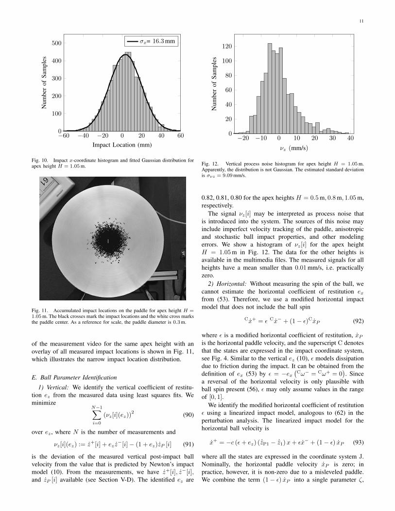
Fig. 12. Vertical process noise histogram for apex height H = 1.05m.Apparently, the distribution is not Gaussian. The estimated standard deviationis σνz = 9.09mm/s.

0.82, 0.81, 0.80 for the apex heights H = 0.5 m, 0.8 m, 1.05 m,respectively.

The signal νz[i] may be interpreted as process noise thatis introduced into the system. The sources of this noise mayinclude imperfect velocity tracking of the paddle, anisotropicand stochastic ball impact properties, and other modelingerrors. We show a histogram of νz[i] for the apex heightH = 1.05 m in Fig. 12. The data for the other heights isavailable in the multimedia files. The measured signals for allheights have a mean smaller than 0.01 mm/s, i.e. practicallyzero.

2) Horizontal: Without measuring the spin of the ball, wecannot estimate the horizontal coefficient of restitution exfrom (53). Therefore, we use a modified horizontal impactmodel that does not include the ball spin

Cx+ = ε Cx− + (1− ε)CxP (92)

where ε is a modified horizontal coefficient of restitution, xPis the horizontal paddle velocity, and the superscript C denotesthat the states are expressed in the impact coordinate system,see Fig. 4. Similar to the vertical ez (10), ε models dissipationdue to friction during the impact. It can be obtained from thedefinition of ex (53) by ε = −ex

(Cω− = Cω+ = 0

). Since

a reversal of the horizontal velocity is only plausible withball spin present (56), ε may only assume values in the rangeof [0, 1].

We identify the modified horizontal coefficient of restitutionε using a linearized impact model, analogous to (62) in theperturbation analysis. The linearized impact model for thehorizontal ball velocity is

x+ = −c (ε+ ez) ( ˙zP1 − ˙z1)x+ εx− + (1− ε) xP (93)

where all the states are expressed in the coordinate system J.Nominally, the horizontal paddle velocity xP is zero; inpractice, however, it is non-zero due to a misleveled paddle.We combine the term (1− ε) xP into a single parameter ζ,

12

−40 −20 0 20 400

200

400

600

νx(mm/s)

Num

ber

ofSa

mpl

esσνx = 15.6mm/s

Fig. 13. Horizontal process noise histogram and fitted Gaussian distributionfor apex height H = 1.05m.

which we identify as well. We minimizeN−1∑i=0

(νx[i](ε, ζ))2 (94)

over ε and ζ, where

νx[i](ε, ζ) := x+[i]+c (ε+ez) ( ˙zP1− ˙z1)x[i]−εx−[i]−ζ. (95)

The measurements provide the ball speeds x+[i] and x−[i],as well as the impact location x[i]. The vertical coefficientof restitution ez is identified in a preceding step (see Sec-tion V-E1) using the vertical data from the same experiment.The nominal values ˙z1 and ˙zP1 are calculated using (6) and(11). Finally, we find ε = 0.70, 0.55, 0.41, and ζ = 6.3,12.7, 7.2 mm/s for apex heights H = 0.5 m, 0.8 m, 1.05 m,respectively.

We show a histogram of the noise signal νx[i] for the apexheight H = 1.05 m in Fig. 13. The signal is zero mean dueto the parameter ζ. We do not state the statistics for the noiseintroduced in the y-direction, as they are practically identical.Measurement data in y, and at other apex heights is availablein the multimedia files provided with this paper.

F. Process Noise Characteristics

We further analyzed the power spectral density functions(PSD) of the measured noise signals νx, νz . We use the PSDsin the parameter optimization presented later on. The powerspectral density function of the signal νx[i] with length N isthe discrete Fourier transform of its autocorrelation function

Sxνν (Ωk) =

N−1∑n=0

Rxνν [n]e−jΩkn (96)

whereΩk =

2πk

N, k = 0, 1, . . . , N − 1 (97)

are the discrete frequencies, and

Rxνν [n] =1

N

N−1∑i=0

νx[i]νx[i− n] (98)

0 π/2 π0

1

2·10−3

Frequency Ω (−)

Sx νν(Ω

)(m

2/s2)

RawSmoothed

Fig. 14. PSD of horizontal process noise νx for apex height H = 1.05m.

0 π/2 π0

1

2

3·10−4

Frequency Ω (−)

Sz νν(Ω

)(m

2/s2)

RawSmoothed

Fig. 15. PSD of vertical process noise νz for apex height H = 1.05m.

is the autocorrelation function. We calculate the autocorrela-tion function with wrap-around, i.e. we assume that the noisesignal is periodic: νx[i + lN ] = νx[i], for any integer l. Weshow the measured PSD for the apex height H = 1.05 m inFig. 14 for the horizontal data, and in Fig. 15 for the verticaldata. In the horizontal PSD, there is a significant amount ofpower present around the frequency Ω = π/2. This is mostlikely due to the spin dynamics which are not captured in themodified horizontal impact model. Evident from both verticaland horizontal PSDs is that the noise signals are not white,since the PSDs are not flat.

VI. DESIGN PARAMETER OPTIMIZATION

For the first prototype of the Blind Juggler, we had to choosefrom a range of stabilizing design parameters. For example,the model predicts that any curvature c ∈ (0, 0.42] keeps theball from falling off the paddle for an apex height of H =

13

1.2 m. But how to choose the specific value? Intuitively, onewould not choose a value that is close to the boundary ofthe stable parameter interval shown in Fig. 6 for reasons of‘robustness’. Another idea would be to choose a curvature thatresults in the smallest spectral radius as, roughly speaking, thespectral radius is a measure for the decay rate of the systemstates. Below, we use a simple scalar dynamical system toshow that both of these intuitions may be misleading, and thatthe spectral radius may not be a good performance metric fora system. Consider the system

x[k + 1] = ax[k] +1

aν[k]

w[k] = x[k] (99)

with state x, noise input ν, output w , and free systemparameter a. We call this system G(a). The goal is to keepthe system output w small in the presence of some processnoise ν. The spectral radius is equal to |a|, and therefore wemay choose any |a| < 1 in order to obtain a stable system.

Considering only the two intuitive criteria stated earlier, wewould choose a = 0, which results in the smallest possiblespectral radius and is also furthest from the boundary of thestable parameter region. However, the process noise enters thesystem through the input gain 1/a, which gets very large forsmall a. Therefore, even though the state decays very quicklyfor small a, the noise is greatly amplified and will producelarge outputs w . A good value for a must therefore be a trade-off between input gain and state decay rate.

We analyze this trade-off for the system (99) with theH2-norm for discrete-time, linear time-invariant (LTI) sys-tems [31]. Roughly speaking, the H2 system norm is the gainof a system if the input is white noise. For example, the H2

norm of the above system is the standard deviation of theoutput w if the noise input ν is unit variance, zero-mean whitenoise. The norm, denoted by subscript H2, is

‖G(a)‖2H2 :=E(w2)

E(ν2)(100)

where E is the expected value. The norm can be calculatedusing the impulse response h[k] of the system:

‖G(a)‖2H2 =

∞∑k=−∞

h2[k] =

∞∑k=1

(1

aak−1

)2

(101)

=1

a2

∞∑k=0

a2k =1

a2 (1− a2). (102)

The trade-off discussed above is reflected in the structure ofthe denominator of the norm. The (1 − a2) factor reflectsthe influence of the spectral radius. In order to achieve alow norm, i.e. low output variance, the factor suggests asmall a. However, there is also the contribution a2 of theinput gain factor, suggesting a large a. The minimizing a isstraightforward to find. It is a∗ =

√2/2 ≈ 0.7. If the process

noise ν was indeed white, it would be optimally rejected bychoosing a = a∗.

A. Output Variance from Input Power Spectral Density

In order to optimize juggling performance by rejectingthe process noise, we use an approach analogous to the H2

analysis in the previous section. We learned from the measure-ments that the process noise cannot be well approximated bywhite noise, see Section V-F. Therefore, we use the measurednoise power spectral densities together with an LTI model ofthe juggling system in order to predict the output variances.Finally, we optimize the system parameters with the objectiveof minimizing the predicted output variances. For example,we analyze the horizontal system, which describes how theprocess noise νx maps to the impact location on the paddle.We then find the paddle curvature that minimizes the predictedvariance of the impact locations.

The variance of the measured noise signal sequence νx[k]of length N may be estimated by

σ2νx =

1

N

N−1∑k=0

ν2x[k] (103)

since the signal has zero mean. This corresponds to thezero-lag value of the autocorrelation function, Rxνν [0] (98).Therefore, we obtain an estimate of the variance from theinverse Fourier transform of the PSD:

σ2νx = Rxνν [0] =

1

N

N−1∑k=0

Sxνν (Ωk) ejΩk·0. (104)

The PSD of the output wx of a single input, single output,discrete-time LTI system Gx may be calculated given the PSDSxνν of the noise input

Sxww(Ωk) = |Gx (Ωk)|2 Sxνν (Ωk) (105)

where |Gx (Ωk) | denotes the magnitude of the frequencyresponse of the system Gx. Using the relation in (104), wemay then estimate the variance of the output (because thesystem is linear and the input is zero-mean, the output is alsozero-mean).

Analogous to the stability analysis in Section IV, we opti-mize the design parameters paddle curvature c and accelerationaP independently for the horizontal and vertical degrees offreedom, as the respective systems are decoupled, to firstorder. Matlab scripts performing the following optimizationsare available in the multimedia files provided with this paper.

B. Optimized Paddle Curvature

We find the paddle curvature c that minimizes the varianceof the impact locations. First, we derive the input-outputrepresentation of the system for the horizontal directions basedon the modified impact model (92) that is governed by themodified horizontal coefficient of restitution ε. We define thediscrete-time LTI system Gx:

X[k + 1] = AεxX[k] + Bxνx[k]

wx[k] = CxX[k].(106)

The state is X = (sx0, sx0)T, the horizontal perturbations at

nominal apex time. The system output wx is equivalent to theimpact location on the paddle, to first order, which is what

14

we want to keep small. The input νx is the horizontal processnoise. The underlying sampling time is 2T , the time betweentwo apexes. The matrices are straightforward to derive from aperturbation analysis analogous to Section III and are

Aεx =

1− 2c(ε+ez)gT 2

ez+1 T(− 2c(ε+ez)gT 2

ez+1 + ε+ 1)

− 2c(ε+ez)gTez+1 ε− 2c(ε+ez)gT 2

ez+1

Bx =

[T1

]Cx =

[1 T

]. (107)

We use the system Gx and the relations (104), and (105) topredict the impact location variance as a function of the paddlecurvature c. We calculate

σ2x (c) =

1

N

N−1∑k=0

Sxww(Ωk, c)

=1

N

N−1∑k=0

|Gx (Ωk, c)|2 Sxνν(Ωk). (108)

We show the magnitude of the frequency response of thesystem, along with the smoothed measured PSD of the noiseinput signal in Fig. 16. We use the standard deviation of theoutput as the objective function to find the optimal noise-rejecting curvature from

mincσx (c) (109)

for apex height H = 1.05 m, and previously identified verticalcoefficient of restitution ez = 0.79 and modified horizontalcoefficient of restitution ε = 0.41. A plot of the standarddeviation σx (c) is shown in Fig. 17. There are two localminima at curvatures of 0.18 (1/m) and 0.39 (1/m). The min-ima are not very pronounced; in the interval c = [0.18, 0.39],the standard deviation is constant and equal to 18 mm whenrounded to millimeters. Therefore, we predict similar impactlocation statistics for all curvatures in this interval.

These results further illustrate the poor correlation betweenthe spectral radius and the system performance. For H =1.05 m we find that the spectral radius of Ax is lowest forc ∈ [0.35, 0.48], see Fig. 6. However, Fig. 17 shows thatfor curvatures above 0.4 (1/m), there is a steep increase inpredicted impact location standard deviation.

Given that the impact location standard deviations areroughly identical for all curvatures in c = [0.18, 0.39], wemay choose a curvature based on other criteria. Namely, weobserve that the worst-case spectral radius analysis in Fig. 6shows that lower paddle curvatures allow juggling at higherapex heights. There is a trade-off between lower curvatures andrequired leveling accuracy, however. The flatter the curvature,the larger the shifts in mean impact location when the paddle ismisleveled. A first-order approximation to the lower bound ∆xof the expected shift in impact location is ∆x = ∆ϑ/c, where∆ϑ (rad) is the leveling error angle. This bound does notinclude the additional shift caused by the non-zero horizontalpaddle velocities due to ∆ϑ. For a curvature of c = 0.18(1/m), a one degree offset would cause the ball to shift atleast 0.1 m.

With the above trade-off in mind, we manufactured a paddlewith a curvature of c = 0.24 (1/m), for which the stability

0 π/2 π

0

0.2

0.4

0.6

0.8

1

1.2·10−3

Frequency Ω (−)

Sx νν(Ω

)(m

2/s2)

0.5

1

1.5

2

|Gx(Ω

)|(s

)

c = 0.18c = 0.26c = 0.39

Fig. 16. Horizontal process noise smoothed power spectral density functionfrom Fig. 14 (gray) and magnitude of frequency responses of the system Gxfor different values of the paddle curvature.

0 0.1 0.2 0.3 0.4 0.517

18

19

20

21

22

Curvature c (1/m)

σx(c)(m

m)

Fig. 17. Objective function of horizontal parameter optimization.

analysis predicts stable juggling at heights of up to 2 m. Weachieved sustained juggling at this height in experiments andshow this in a video provided with the paper.

C. Optimized Paddle Acceleration

Analogous to the paddle shape optimization, we optimizethe paddle acceleration aP to minimize the standard deviationof the apex height. We define the discrete-time LTI system Gz:

Z[k + 1] = AzZ[k] + Bzνz[k]

wz[k] = CzZ[k].(110)

The state is Z = (sz0, sz0)T, the vertical perturbations at

nominal apex time. The output corresponds to the apex heightdeviation, to first order, which is equivalent to sz0. Theunderlying sampling time is 2T . We reuse Az (79) from theperturbation analysis. The other system matrices are

Bz =

[T1

], Cz = [1, 0] . (111)

15

We predict the output variance analogously to before (108):

σ2z (aP) =

1

N

N−1∑k=0

Szww(Ωk, aP)

=1

N

N−1∑k=0

|Gz (Ωk, aP)|2 Szνν(Ωk). (112)

We show the magnitude of the frequency response of thesystem, along with the smoothed measured PSD of the noiseinput signal in Fig. 18. We obtain aP = −1.75 m/s2 from

minaP

σz (aP) (113)

for apex height H = 1.05, and previously identified verticalcoefficient of restitution ez = 0.80. A plot of the standarddeviation σz (aP) is shown in Fig. 19. The minimized standarddeviation is σz = 4.3 mm. The standard deviation for aP =−g/2 ≈ −4.9 m/s2 is 6.8 mm, thus the predicted improvementis 37% using the optimized acceleration.

In an experiment, we gathered impact data for aP =−1.75 m/s2 using the same ball and paddle as for the mea-surements at aP = −g/2 presented in Table I. The mea-sured apex height standard deviation is σz = 4.0 mm with95%-confidence interval of [3.88, 4.22]. Given the measuredstandard deviation for aP = −g/2 of σz = 5.5 mm, theimprovement is 27%.

The process noise power spectral density measured ataP = −1.75 m/s2 is, not surprisingly, different from thespectrum measured at aP = −g/2. A contributing factoris that the paddle velocity tracking errors depend on thedesired paddle acceleration aP. In addition, different precisionballs produce different noise spectra. With the new measurednoise power spectrum, we could repeat the optimization, findthe optimal acceleration, and obtain new measurements. Thiscould be extended into an iterative scheme with no guaranteesof convergence to an optimal paddle acceleration. Since themeasured spectra depend on a range of system parameters,and since the optimized vertical juggling performance isacceptable, we did not pursue this strategy further.

Finally, even though the measured improvement of 27% islarge, it is hardly noticeable when watching the Blind Jugglerbounce a ball. A higher deceleration is in fact often preferable,as it allows the robot to juggle balls with a larger range ofcoefficients of restitution, see the discussion in Section V-A.A video demonstrating the high vertical juggling performancewith a close-up of ball apexes, for both aP = −g/2 and aP =−1.75 m/s2, is available in the multimedia files provided withthis paper.

VII. CONCLUSIONS

The Blind Juggler demonstrates that high-performancerobotic juggling of unconstrained balls is possible withoutfeedback. We analytically showed local stability of the balltrajectory and verified the results in experiments that confirmedthe robot’s ability to continuously juggle balls at heights ofup to 2 m. We would like to highlight how signal process-ing concepts, such as predicting system performance frommeasured noise power spectral densities, may be used for

0 π/2 π

0

1

2

3

·10−4

Frequency Ω (−)

Sz νν(Ω

)(m

2/s2)

0

0.5

1

1.5

2

|Gz(Ω

)|(s

)

aP = −1.7aP = −4.9aP = −7.0

Fig. 18. Vertical process noise smoothed power spectral density functionfrom Fig. 15 (gray) and magnitude of frequency responses of the system Gzfor different values of the paddle acceleration.

−10 −8 −6 −4 −2 00

5

10

15

20

Paddle Acceleration aP (m/s2)

σz(a

P)(m

m)

Fig. 19. Objective function of vertical parameter optimization.

optimizing hardware design. The procedure of building afirst prototype, obtaining noise measurements, and subsequentdesign optimization may be useful for other mechanical robotdesigns.

The results obtained with the Blind Juggler allow us todesign more advanced juggling robots, for example the Pen-dulum Juggler, which is able to juggle unconstrained ballsin a side-to-side pattern without feedback [32]. We furtherdeveloped a paddle that features four concave, parabolic areaswhich enables the Blind Juggler to simultaneously juggleup to four balls. We use this paddle to study the richdynamics of the bouncing ball system, such as co-existingstable periodic orbits and chaotic system behavior. Additionalinformation, including videos, may be found on the projectwebsite: www.blindjuggler.org.

ACKNOWLEDGEMENTS

We would like to thank Matthew Donovan and Daniel Burchfor their great help with the mechanical and electrical design

16

of the Blind Juggler. We further thank Matthias Fassler forhis help with the measurement setup. Lastly, we are indebtedto the anonymous reviewers and Sebastian Trimpe for theirvaluable suggestions and comments.

REFERENCES

[1] P. Reist and R. D’Andrea, “Bouncing an Unconstrained Ball in ThreeDimensions with a Blind Juggling Robot,” in Proc. IEEE Int. Conf.Robotics and Automation (ICRA), 2009.

[2] P. J. Holmes, “The dynamics of repeated impacts with a sinusoidallyvibrating table,” Journal of Sound Vibration, vol. 84, Sep. 1982.

[3] N. B. Tufillaro, T. Abbot, and J. Reilly, An experimental approach tononlinear dynamics and chaos. Addison-Wesley, 1992.

[4] T. L. Vincent, “Control using chaos,” IEEE Control Systems Magazine,vol. 17, no. 6, 1997.

[5] M. Buehler, D. E. Koditschek, and P. J. Kindlmann, “A Simple JugglingRobot: Theory and Experimentation,” in Proc. Int. Symp. Exp. Robotics,1990.

[6] ——, “A Family of Robot Control Strategies for Intermittent DynamicalEnvironments,” in Proc. IEEE Int. Conf. Robotics and Automation(ICRA), 1989.

[7] A. A. Rizzi and D. E. Koditschek, “Further progress in robot juggling:solvable mirror laws,” in Proc. IEEE Int. Conf. Robotics and Automation(ICRA), 1994.

[8] S. Schaal and C. G. Atkeson, “Open loop stable control strategies forrobot juggling,” in Proc. IEEE Int. Conf. Robotics and Automation(ICRA), 1993.

[9] S. Schaal, D. Sternad, and C. G. Atkeson, “One-handed juggling: Adynamical approach to a rhythmic movement task,” Journal of MotorBehavior, 1996.

[10] G. Baetz, M. Sobotka, D. Wollherr, and M. Buss, “Robot Basketball:Ball Dribbling – A Modified Juggling Task,” in Advances in RoboticsResearch. Springer, 2009.

[11] R. P. Ringrose, “Self-stabilizing running,” Ph.D. dissertation, Mas-sachusetts Institute of Technology, Cambridge, MA, 2008.

[12] R. R. Burridge, A. A. Rizzi, and D. E. Koditschek, “Sequential Com-position of Dynamically Dexterous Robot Behaviors,” Int. J. Rob. Res.,vol. 18, no. 6, 1998.

[13] A. A. Rizzi and D. E. Koditschek, “Further progress in robot juggling:the spatial two-juggle,” in Proc. IEEE Int. Conf. Robotics and Automa-tion (ICRA), 1993.

[14] P. Kulchenko and E. Todorov, “First-exit model predictive control of fastdiscontinuous dynamics : Application to ball bouncing,” in Proc. IEEEInt. Conf. Robotics and Automation (ICRA), 2011.

[15] R. G. Sanfelice, A. R. Teel, and R. Sepulchre, “A Hybrid SystemsApproach to Trajectory Tracking Control for Juggling Systems,” in Proc.IEEE Conf. Decision and Control (CDC), 2007.

[16] A. Zavala-Rio and B. Brogliato, “On the control of a one degree-of-freedom juggling robot,” Dyn. Control, vol. 9, no. 1, 1999.

[17] S. Schaal and C. G. Atkeson, “Robot juggling: implementation ofmemory-based learning,” IEEE Control Systems Magazine, vol. 14,no. 1, 1994.

[18] T. Sakaguchi, M. Fujita, H. Watanabe, and F. Miyazaki, “Motionplanning and control for a robot performer,” in Proc. IEEE Int. Conf.Robotics and Automation (ICRA), 1993.

[19] R. Ronsse, P. Lefevre, and R. Sepulchre, “Timing Feedback Control ofa Rhythmic System,” in Proc. IEEE Conf. Decision and Control andEuropean Control Conf. (CDC-ECC), 2005.

[20] ——, “Sensorless stabilization of bounce juggling,” IEEE Transactionson Robotics, vol. 22, no. 1, 2006.

[21] R. Ronsse and R. Sepulchre, “Feedback Control of Impact Dynamics:the Bouncing Ball Revisited,” in Proc. IEEE Conf. Decision and Control(CDC), 2006.

[22] R. Ronsse, P. Lefevre, and R. Sepulchre, “Rhythmic Feedback Controlof a Blind Planar Juggler,” IEEE Transactions on Robotics, vol. 23,no. 4, 2007.

[23] D. Hobbelen and M. Wisse, “Swing-Leg Retraction for Limit Cy-cle Walkers Improves Disturbance Rejection,” IEEE Transactions onRobotics, vol. 24, no. 2, 2008.

[24] ——, “A disturbance rejection measure for limit cycle walkers: The gaitsensitivity norm,” IEEE Transactions on Robotics, vol. 23, no. 6, 2007.

[25] K. D. Mombaur, H. G. Bock, J. P. Schloder, and R. W. Longman, “Open-loop stability - a new paradigm for periodic optimal control and analysisof walking mechanisms,” in Proc. IEEE Int. Conf. Robotics, Automationand Mechatronics (RAM), 2004.

[26] R. Cross, “Grip-slip behavior of a bouncing ball,” American Journal ofPhysics, vol. 70, no. 11, 2002.

[27] S. H. Strogatz, Nonlinear Dynamics And Chaos, 1st ed. Perseus BooksGroup, 1994.

[28] G. Strang, Linear Algebra and Its Applications. Addison Wesley, 1988.[29] “LinMot Website.” [Online]. Available: www.linmot.com[30] “D-Space Website.” [Online]. Available: www.dspace.de[31] S. Skogestad and I. Postlethwaite, Multivariable Feedback Control.

Wiley, 2007.[32] P. Reist and R. D’Andrea, “Design of the Pendulum Juggler,” in Proc.

IEEE Int. Conf. Robotics and Automation (ICRA), 2011.

Philipp Reist received the B.Sc. and M.Sc. degree inMechanical Engineering from ETH Zurich in 2007and 2008, and was awarded the “Outstanding D-MAVT Bachelor Award” for his B.Sc. GPA. Duringhis studies, he was part of the ETH team that wonthe Atlanta RoboCup Nanogram tournament, andspent two semesters at the Massachusetts Instituteof Technology, where he worked on an underwaterrangefinder and on randomized feedback motionplanning. Since 2009, he has been a graduate studentat the Institute for Dynamic Systems and Control at

ETH Zurich. His research interests include control of dynamical systems,nonlinear dynamics, and mechanism design. In addition to research, heregularly teaches robotics workshops for high school students.

Raffaello D’Andrea received the B.Sc. degree inEngineering Science from the University of Torontoin 1991, and the M.S. and Ph.D. degrees in ElectricalEngineering from the California Institute of Technol-ogy in 1992 and 1997. He was an assistant, and thenan associate, professor at Cornell University from1997 to 2007. While on leave from Cornell, from2003 to 2007, he co-founded Kiva Systems, wherehe led the systems architecture, robot design, robotnavigation and coordination, and control algorithmsefforts. A creator of dynamic sculpture, his work has

appeared at various international venues, including the National Gallery ofCanada, the Venice Biennale, Ars Electronica, the Smithsonian, the FRACCentre, and the Spoleto Festival. He is currently professor of DynamicSystems and Control at ETH Zurich and chief technical advisor at KivaSystems.