DESIGN AND ANALYSIS OF A LABVIEW AND ARDUINO-BASED AUTOMATIC

SOLAR TRACKING SYSTEM

__________________________

A Thesis

Presented to

the Faculty of the College of Science and Technology

Morehead State University

_________________________

In Partial Fulfillment

of the Requirements for the Degree

Master of Science

_________________________

by

Caiwen Ding

April 24, 2015

All rights reserved

INFORMATION TO ALL USERSThe quality of this reproduction is dependent upon the quality of the copy submitted.

In the unlikely event that the author did not send a complete manuscriptand there are missing pages, these will be noted. Also, if material had to be removed,

a note will indicate the deletion.

Microform Edition © ProQuest LLC.All rights reserved. This work is protected against

unauthorized copying under Title 17, United States Code

ProQuest LLC.789 East Eisenhower Parkway

P.O. Box 1346Ann Arbor, MI 48106 - 1346

UMI 1587336Published by ProQuest LLC (2015). Copyright in the Dissertation held by the Author.

UMI Number: 1587336

Accepted by the faculty of the College of Science and Technology, Morehead State University,

in partial fulfillment of the requirements for the Master of Science degree.

____________________________

Dr. Yuqiu You

Director of Thesis

Master’s Committee: ________________________________, Chair

Dr. Ahmad Zargari

_________________________________

Dr. Yuqiu You

_________________________________

Dr. Hans Chapman

________________________

Date

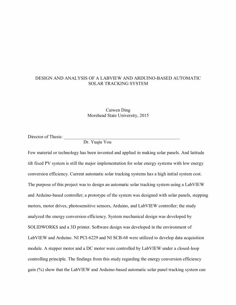
DESIGN AND ANALYSIS OF A LABVIEW AND ARDUINO-BASED AUTOMATIC

SOLAR TRACKING SYSTEM

Caiwen Ding

Morehead State University, 2015

Director of Thesis: __________________________________________________

Dr. Yuqiu You

Few material or technology has been invented and applied in making solar panels. And latitude

tilt fixed PV system is still the major implementation for solar energy systems with low energy

conversion efficiency. Current automatic solar tracking systems has a high initial system cost.

The purpose of this project was to design an automatic solar tracking system using a LabVIEW

and Arduino-based controller; a prototype of the system was designed with solar panels, stepping

motors, motor drives, photosensitive sensors, Arduino, and LabVIEW controller; the study

analyzed the energy conversion efficiency. System mechanical design was developed by

SOLIDWORKS and a 3D printer. Software design was developed in the environment of

LabVIEW and Arduino. NI PCI-6229 and NI SCB-68 were utilized to develop data acquisition

module. A stepper motor and a DC motor were controlled by LabVIEW under a closed-loop

controlling principle. The findings from this study regarding the energy conversion efficiency

gain (%) show that the LabVIEW and Arduino-based automatic solar panel tracking system can

increase the energy conversion efficiency significantly. This study can be a systematic

foundation for future works to continue to build upon.

Accepted by: ______________________________, Chair

Dr. Ahmad Zargari

______________________________

Dr. Yuqiu You

_________________________________

Dr. Hans Chapman

ACKNOWLEDGEMENT

First and foremost, I would like to appreciate all the professors and staff who helped me

with this thesis at the AET department. I would like to offer my sincere thanks and appreciation to

my Thesis Director, Dr. Yuqiu You for her support from the beginning of the Master’s program

and her guidance throughout the research. I have learned a great deal in the time spent working on

this research and project. The success of this thesis would not have been possible without her

elaborate support and mentorship.

I also extend my sincere thanks to Dr. Ahmad Zargari for pushing me forward and his

insightful comments and encouragement as a committee member. I would like to thank Dr. Hans

Chapman for his support and assistance throughout my thesis process. All the committee

members’ expertise and guidance played a significant role in the completion of the thesis.

In addition, a thank you to my brother, Mr. Caiwu Ding, for his 3D model computer-aided

design.

I sincerely thank my parents for everything they did for me. What I have accomplished

would not have been possible without their continued and unwavering support. I cannot express

my appreciation enough for their dedication.

TABLE OF CONTENTS

CHAPTER I- INTRODUCTION ................................................................ 1

Overview ............................................................................................................................................. 1

Statement of the Problem ..................................................................................................................... 3

Objectives ........................................................................................................................................... 4

Assumptions ........................................................................................................................................ 5

Limitations and Geographical Focus: ................................................................................................... 5

Definition of Terms ............................................................................................................................. 6

Significance of the Study ..................................................................................................................... 8

CHAPTER II- REVIEW OF LITERATURE ............................................ 9 Solar Energy ........................................................................................................................................ 9

Solar Tracking System ....................................................................................................................... 11

Software Review ............................................................................................................................... 13

CHAPTER III- METHODOLOGY.......................................................... 16 Restatement of the Research Objective .............................................................................................. 16

Strategy of First Objective ................................................................................................................. 16

Strategy of Second Objective ............................................................................................................. 18

Strategy of Third Objective ................................................................................................................ 25

CHAPTER IV- FINDINGS ....................................................................... 29 Discussion of Objective One .............................................................................................................. 29

Discussion of Objective Two ............................................................................................................. 37

Discussion of Objective Three ........................................................................................................... 44

CHAPTER V- CONCLUSION, RECOMMENDATIONS, AND

FUTURE RESEARCH .............................................................................. 53

Conclusion ........................................................................................................................................ 53

Recommendations ............................................................................................................................. 54

Future Research ................................................................................................................................. 54

REFERENCES........................................................................................... 56

APPENDIX ................................................................................................. 59

1

CHAPTER I- INTRODUCTION

Overview

The energy crisis has been one of the most important issues in today’s world. Renewable

energy sources have earned a high priority in reducing dependency on conventional sources. Solar

energy system are quickly becoming the major renewable source to replace the conventional energy

sources due to its inexhaustibility and its environmental implications.

Humans have used fossil fuels which took millions of years to form and was stored in the

ground in various places. Humans now must put an extreme effort, technologically and politically,

into finding new energy systems that uses solar energy more directly. Being one of the most

inspiring challenges facing engineers and scientists today, Photovoltaic (PV) is one of the exciting

new technologies that is already helping us towards a solar future. (Lynn, P., 2010).

Global primary energy consumption increased by 2.3% in 2013, and by 1.8% in 2012. Growth

in 2013 resulted from the consumption of oil, coal, and nuclear power, but global growth remained

below the 10-year average of 2.5%. All fuels except oil, nuclear power and renewables in power

generation grew at below-average rates. All regions, except North America, were below the growth

average. Oil remains the world’s leading fossil fuel, comprising 32.9% of global energy

consumption, although it continued to lose its market share for the fourteenth consecutive year and

the current market share remains the lowest in the data set, which began in 1965. (BP Statistical

Review of World Energy 2014, 2014)

PV’s earliest applications were in situations where there was a lack of electricity. While the

cost has decreased and the efficiency of PV has increased, more applications involving PV have

emerged. With greater demands on developing the technology and increasing, the production of

2

PV systems has been implicated toward cost performance in a wide range of PV applications.

In the new solar age, people apply PV applications to places that need electricity. Being

versatile, PV applications also support AC circuits and DC circuits, can also be grid-connected.

Current PV systems include photovoltaic modules, inverters modules, storage batteries, and

control components. Supply chain refers to the procurement of all required inputs, conversion into

finished PV products, distribution, and installation of these products for customers. The value

chain looks at how increased customer value can be created across a company’s business activities,

which can include design, production, marketing, delivery, and support functions. (TRENDS in

Photovoltaic Applications – 2013.)

There are four primary applications for PV power systems:

1. Off-grid domestic systems provide electricity to households and villages that are not

connected to a utility electricity network (also referred to as the grid). They provide

electricity for lighting, refrigeration and other low power loads. These have been installed

worldwide and are often the most appropriate technology to meet the energy demands of

off- grid communities. Off-grid domestic, Grid-connected distributed PV systems are

installed to provide power to a grid-connected customer or directly to the electrical

network. Such systems may be integrated into the customer’s residence often on the

demand side of the electricity meter. The PV Systems are typically around 1 kW in size

and generally offer an economic alternative to extending the electricity distribution

network at distances of more than 1 or 2 km from existing power lines. Defining such

systems is becoming more difficult where, for example, mini-grids in rural areas are

developed by electricity utilities.

2. Off-grid non-domestic installations were the first commercial application for terrestrial

3

PV systems. They provide power for a wide range of applications, such as

telecommunication, water pumping, vaccine refrigeration, and navigational aids. These

are applications where small amounts of electricity have a high value, making PV

commercially cost competitive with other small generating sources.

3. Grid-connected distributed PV systems are installed to provide power to a grid-connected

customer or directly to the electrical network, specifically where the part of electrical

network is configured to supply power to a number of customers. Such systems may be

integrated into the customer’s premises often on the demand side of the electricity meter,

on public and commercial buildings, or simply built into the environment or on motorway

sound barriers, etc. Size is not a determining feature – while a 1 MW PV system on a

roof-top may be large by PV standards, this is not the case for other forms of distributed

generation.

4. Grid-connected centralized systems perform the functions of centralized power stations.

The power supplied by such a system is not associated with a particular electricity

customer. The system is not located to specifically perform functions on the electricity

network other than the supply of bulk power. These systems are typically ground-

mounted and functioning independently of any nearby development.

Statement of the Problem

In a solar energy system, solar panels are used to directly convert solar radiation into

electrical energy. Solar panels are made from semiconductor materials which has a maximum

efficiency of 12% in energy conversion (DOE). Unless a new material or technology is invented

and applied in making solar panels, the most cost-effective method to improving the efficiency of

solar panels is to increase light intensity.

4

A Latitude tilt fixed PV system is still the major implementation for solar energy systems

with low energy conversion efficiency, especially for small-scale household systems.

Automatic solar tracking systems have been designed and studied by many researchers.

However, most applied solar tracking systems are either too expensive in an industrial scale or small

capacity at laboratory level with a shortcoming of high cost or low accuracy. Fixed solar panels are

still the major implementation for solar energy systems, especially for small-scale household

system.

Objectives

In a solar energy system, solar panels are used to directly convert solar radiation into

electrical energy. Solar panels are made from semiconductor materials which have a maximum

efficiency of 12% in energy conversion (DOE). Unless a new material or technology is invented

and applied in making solar panels, the most cost-effective method to improving the efficiency of

solar panels is to increase light intensity.

The research will try to answer the following questions: What is the feasibility of an

automatic solar tracking system? What design and specific architecture is needed for a solar

tracking system that is at the lowest cost and the highest accuracy relative to residential needs? How

much more electricity can be converted in the solar tracking system when compared to the latitude

tilt fixed PV system?

Three objectives are posed to answer the questions:

1. Design an automatic solar tracking system using a LabVIEW and Arduino-based

controller.

2. Design a prototype of the system with solar panels, stepping motors, motor drives,

photosensitive sensors, Arduino, and LabVIEW controller.

5

3. Analyze the energy conversion efficiency gain.

Assumptions

1. The solar tracking power system operated under daylight lamp in a laboratory. The gain of

the energy conversion efficiency of the solar resources will be same as the measurement at

the lab.

2. The energy efficiency figures calculated by DOE are accurate and represent a standard of

all the states.

3. The data measured through multi-meters and DAYSTAR DS-05 SOLAR IRRADIANCE

METER had an accuracy to support the data analysis and conclusion.

4. The calculation of cost for the solar tracking system will be based on the current price of

equipment.

Limitations and Geographical Focus:

Solar energy is an effective source of energy with near limitless potential. However this source

of energy does incur significant limitations even with the advantages of solar tracking. The major

limitation in implementing this technology would be the location. For example the mountainous

regions of Eastern Kentucky are not suitable for solar energy. The tracking system can help mitigate

this limitation, however the region’s dense forest may cause the technology to be prohibitive.

An idea location for solar energy would be a locale that receives a significant amount of solar

energy; ideally throughout the entire solar year. These locations do exist within the United States.

According to Huffing post the top ten solar cities by total installed PV capacity are “Lost Angeles,

San Diego, CA, San Diego, CA, Phoenix, AZ, Honolulu, HI, San Antonio, TX, Indianapolis, IN,

New York, NY, San Francisco, CA and Denver CO” (Fox, 2014). The majority of these locations

6

are in California and the southern regions of the United States. These locations receive an ample

amount of solar energy due to the climate. California has the Mediterranean climate; the southern

areas are within the humid subtropical climate zones. (Alt, M., 2015)

These two climate zones the Mediterranean and subtropical climate zones are idea for solar

energy. The Mediterranean climate features “relatively low annual rainfall with high solar

intensity” (Characteristics of Mediterranean Climates, 1973). It is this climate condition which makes

it conducive to solar power. The other climate zone the sub humid tropic climate zone has a fairly

substantial growing season. This growing season last for about eight months (Climatic). Which

indicates a fairly high solar intensity environment with ample precipitation Solar panels are

designed to reserve energy as well. Therefore it is also this type of climate zone which is ideal for

solar energy.

In the United States locations within the sub humid tropical and Mediterranean climate zones

are ideal for solar energy. This is due to these particular locations receiving abundant solar inputs.

The limitations of the study are as follow:

1. The operation including data acquisition and motor motion of the solar panel tracking

system highly depend on a PC equipped with LabVIEW 2011 and NI PCI-6229

2. The cost comparing and energy conversion efficiency of this study are reflective of US costs

only.

3. The solar tracking system is operated as an off-grid power system and not be connected to

the main or national electrical grid.

4. The solar panel tracking system could not be operated normally the extreme weather.

Definition of Terms

PV System: A solar power system designed to supply solar power by using photovoltaics.

7

DOE: The United Stated Department of Energy.

DC Motor: Also named direct current motor. It is an electrical machine that used to convert the

power of direct current (DC) into mechanical power form to drive objectives.

Stepper Motor: A brushless DC electric motor that contains a permanent magnet rotor and a poly-

phase coil stator.

LabVIEW: NI LabVIEW system design software is at the center of the National Instruments

platform. Providing comprehensive tools that you need to build any measurement or control

application in dramatically less time, LabVIEW is the ideal development environment for

innovation, discovery, and accelerated results. (www.ni.com/labview/why/)

Solar Tracking System: a device designed for concentrating a solar panel towards the sun.

Single Axis Tracking System: Solar panel with single axis tracker that can turn around the center

axis. A single axis tracking system is normally a latitude tilt fixed PV system.

Double/ Dual Tracking System: used to track the sun on both axis (according to azimuth and solar

altitude angles).

NI PCI-6229: The National Instruments PCI-6229 is a low-cost multifunction M Series data

acquisition (DAQ) board optimized for cost-sensitive applications.

NI SCB-68: Shielded I/O Connector Block for DAQ Devices with 68-Pin Connectors.

Arduino: is an open-source electronics platform based on easy-to-use hardware and software.

Minitab: is a statistic software that often used for statistic-based process improvement methods.

Off-grid Power System: An off-grid power system can be a stand-alone system (SHS) or a mini-

grid that is not connected to the main or national electrical grid.

The Reliability of Power Supply: refers to the electricity supply ability of a power system. The

calculation of reliability value is: the number of hours the system supplies stable electricity per year

8

÷ (24×365).

Photoelectric Sensor: A photoelectric sensor is a device that detects a change in light intensity.

Significance of the Study

The Solar tracking system generates more electricity than their stationary counterparts-

latitude tilt fixed PV system due to an increased direct exposure to solar rays.

Arduino has the hardware platform; it allows programming and serial communication over

USB. LabVIEW has the Real-Time Module to implement high-performance real-time applications.

Arduino and LabVIEW have the reliability and capability to create powerful distributed motion

control solutions.

With the characteristic of solar energy’s inexhaustibility and its environmental implications,

the automatic solar tracking system can significantly improve the energy conversion efficiency and

benefit the environment.

9

CHAPTER II- REVIEW OF LITERATURE

In this chapter, a brief history of solar power generation and solar tracking systems will be

discussed. Related literature will be reviewed and discussed.

Solar Energy

Solar energy is an inexhaustible and environmentally friendly source. Humans had started to

try to harvest sun energy since long time ago. Also, people utilize solar energy in many other

indirectly different ways. For example, people discovered fossil energy and how to transform it into

transportation and electricity. Fossil energy is a stored solar energy from millions years ago.

Additionally, biomass-energy converts the solar energy into a fuel that can be used for heat.

In 1767, Horace de Saussure, a Swiss Physicist, invented the first solar oven by building glass

boxes. Then in the 1830’s, Sir John Herschel, the noted astronomer, made a solar cookout. (Horace

de Saussure and his hot boxes of the 1700's, 2004)

A French physicist, Edmond Becquerel (1820-1891) was famous for his studies in the solar

spectrum, magnetism, electricity and optics in 1839. He was only 19 years old at the time,

discovered that there is a creation of voltage when a material is exposed to light his discovery laid

the principle to solar energy cells, the photovoltaic effect. (Zamostny, D., 2011)

In 1873, Willoughby Smith, an English engineer, discovered the photoconductivity in solid

selenium, a known metal of very high resistance. (Smith, W, 1873).

In 1876, William Grylls Adams and his students, Richard Evans Day discovered that selenium

produces small amounts of electricity when exposed to light. (History of Solar Energy in California,

1999)

10

In 1883, an American inventor, Charles Fritts was the first person that discovered the first

solar cells based on selenium wafers. (Fritts,C.E., 1883)

In a famous paper published in 1905, Einstein postulated that light had an attribute that had

not yet been recognized. Einstein said light contains packets of energy which he called light quanta

(now called photons). In 1921, 16 years after he submitted this paper, he was awarded the Nobel

Prize for the scientific breakthroughs he had discovered. (Early Solar History, 1999)

In 1918, Polish scientist Jan Czochralski discovered a way to produce single-crystal silicon.

His first discovery in the beginning of the 20th century was rediscovered later in the middle of the

century by American semiconductor technology specialists, who named his crystal pulling

technique “the Czochralski method”. The Czochralski method of growing single crystals brought

Jan Czochralski his greatest publicity. The method was developed in 1916 and was initially used to

measure of crystallization rate of metals. The method was developed as a result of an accident and

through Czochralski's careful observation. (Tomaszewski, P., 1998)

In 1954, Bell laboratories developed the first inorganic photovoltaic cells. David Chapin,

Calvin Fuller and Gerald Pearson of Bell Labs are famous for the world’s first photovoltaic cell

(solar cell). In other words, they are the first men that made the first device that converted sunlight

into electrical power. (D. M. Chapin, 1954).

In 1981, Paul Macready produced the first solar powered aircraft. The aircraft used more than

1600 cells, placed on its wings. The aircraft flew from France to England.

In the year 1982, there was the development of the first solar powered cars in Australia. (History of

Solar Energy, 2012)

In the past few years, enormous investment in utility-scale solar plants have been seen with

records for the largest frequently being broken. As of 2012, the largest solar energy plant is the

11

Golmud Solar Park in China, with an installed capacity of 200 megawatts. This is arguably

surpassed by India’s Gujarat Solar Park, a collection of solar farms scattered around the Gujarat

region, boasting a combined installed capacity of 605 megawatts. (History of Solar Energy)

Solar Tracking System

A PV cell can be modeled by a current source in parallel with a diode, with resistance in series

and shunt (parallel) as shown in Figure 2.1. Both series and shunt resistances have a strong effect

on the shape of the I-V curve. Series resistance in PV devices includes the resistance of a cell, its

electrical contacts, module interconnections, and system wiring. These resistances are in addition

to the resistance in a PV system is unavoidable because all conductors have some resistance.

However, increasing series resistance can indicate problems with electrical connections. (Dunlop,

J., 2010).

Figure 2.1 Single-diode mathematical model of a PV cell

In 1975, McFee presented one of the first automatic solar tracking systems, in which he

subdivided each plane-mirror into 484 elements, assuming the slope of each element to be

representative of the surface slope average at its location, and summing the contributions of all

elements and then of all mirrors in the array. For a given sun location and set of array parameter

values, he computed the total received power and flux density distribution. (McFee, R.H., 1975).

Semma and imamru, in 1980, used a simple microprocessor to adjust the positions of the solar

tracker so that the solar panel can toward the sun at all times (Semma, 1980).

Maish, in 1990, developed a SolarTrak control system to provide sun tracking, night and

12

emergency stow, communication, and manual drive control functions for one and two-axis solar

trackers in a low-cost, user-friendly package. He used a six-degree self-alignment routine and a

self-adjusting motor actuation time as control algorithms in order to improve both the SolarTrack’s

pointing accuracy and the system reliability. The results of his study showed that the control system

achieved a full day pointing accuracy. (Maish, 1990)

Dolara points out in his paper that solar tracking system is one of the most effective approaches

to harvest solar energy from the sun compared to fixed solar panels. Solar tracker follows the

position of the sun over the course of the day from east to west in a daily and seasonal basis. Hence,

the PV panels able to receive maximum sunlight and generate more energy. Dolara proposes and

analyzes a single-axis tracking system, studies the efficiency of single-axis system based on his

experimental results of a specific power plant. Experimental data have been collected by an on-site

monitoring system over a period of one year, bringing some final considerations and comparative

results on PV-system efficiency. (Dolara, 2012)

Eku analyzed a double axes sun tracking photovoltaic (PV) systems after one year of

operation. The performance measurements of the PV systems were carried out first when the PV

systems were in a fixed position and then the PV systems were controlled while tracking the sun in

two axes (on azimuth and solar altitude angles) and the necessary measurements were performed.

It is calculated that 30.79% more PV electricity is obtained in the double axis sun-tracking system

when compared to the latitude tilt fixed system. The difference between the simulated and measured

energy values are less than 5%. However, he did not give the architecture and cost of the solar

tracking system. Also all the calculations were based on the software PVSYST 2009. (Eke, R.,

2012).

Sherwood points out in his paper that solar power in Kentucky has been growing in recent

13

years because of the new technological improvements and a variety of regulatory actions. For any

size renewable energy project, the financial incentives have a 30% federal tax credit. Covering just

one-fifth of Kentucky with photovoltaic cells would supply the power to all of Kentucky.

(Sherwood, 2012)

Software Review

In this study, LabVIEW 2011 and Arduino served as the simulation environment and the actual

controller. With the development of technology, the measurement field develops rapidly for

measurement. With the development of technology, the measurement field develops rapidly. It has

evolved from the earliest analog meters based on electro-magnetic induction to a microprocessor-

based intelligent instrumentation. However, with the emergence of virtual instrument, the

development of measure technology has entered a new era. LabVIEW software is ideal for any

measurement or control system. Integrating all the tools that engineers and scientists need to build

a wide range of applications in dramatically less time, LabVIEW is a development environment for

problem solving, accelerated productivity, and continual innovation. (One Platform, Infinite

Possibilities, 1999)

The kernel of LabVIEW is to combine traditional measure instruments and computer software

in order to implement measurement. For control systems built through LabVIEW, peripheral

hardware are merely to provide channels for data transmissions, system software are the kernel for

control systems. For customers, the function of LabVIEW can be modified through block diagrams

which can allow customers to design their own virtual instrument platform with their own ideas.

14

Figure 2.2 Schematic of Virtual instrument systems

Figure 2.2 is the structure of virtual instrument system. The core functionality involves

detecting signals pass through I/O interfacing devices, signal circuit modifications, filtering, A/D

processing, configuring data acquisition, acquiring data. After transferring data to computer through

bus line, logging data to disk, displaying data, computer will complete the data acquisition and

displaying, testing and analyzing. In addition, compared to the microprocessor to process data,

virtual instruments implement data processing through computer. Thus the data processing of

virtual instruments is faster than microprocessor.

Now, with the emergence and development of solar technology, due to the virtual instrument

with the advantage of strong interchangeable and low cost, virtual instruments are gradually applied

to the solar tracking system.

Arduino is an open-source electronics platform based on easy-to-use hardware and software.

It is designed for anyone making interactive projects. The Arduino Uno is a microcontroller board

based on the ATmega328 (datasheet). It has 14 digital input/output pins (of which 6 can be used as

PWM outputs), 6 analog inputs, a 16 MHz ceramic resonator, a USB connection, a power jack, an

ICSP header, and a reset button. It contains everything needed to support the microcontroller;

simply connect it to a computer with a USB cable or power it with an AC-to-DC adapter or battery

to get started. (What is Arduino? 2015)

Detection Targets

Signal Modifications

Data Acquisition

Data Processing

Virtual Instrument Panel

15

As a low cost motion controller, Arduino has a variety of features including:

Using an Arduino simplifies the amount of hardware and software development you need to

do in order to get a system running.

The Arduino hardware platform already has the power and reset circuitry setup as well as

circuitry to program and communicate with the microcontroller over USB. In addition, the I/O pins

of the microcontroller are typically already fed out to sockets/headers for easy access.

On the software side, Arduino provides a number of libraries to make programming the

microcontroller easier. The simplest of these are functions to control and read the I/O pins rather

than having to fiddle with the bus/bit masks normally used to interface with the ATmega I/O. More

useful are things such as being able to set I/O pins to PWM at a certain duty cycle using a single

command or doing Serial communication.

The most convenient advantage is that Arduino has the hardware platform set up already; it

allows programming and serial communication over USB.

16

CHAPTER III- METHODOLOGY

Restatement of the Research Objective

In this chapter, the methods of system design including the software interface and hardware

design was presented. The software interface contained data acquisition and motor motion sections.

The hardware design contained the system frame, mechanical driver parts, DC motors and stepper

motors and motor’s driver.

In the present research, three research objectives were going to be solved regarding the design

and analysis of a LabVIEW and Arduino-based automatic solar tracking system:

1. Design an automatic solar tracking system using a LabVIEW and Arduino-based

controller.

2. Design a prototype of the system with solar panels, stepping motors, motor drives,

photosensitive sensors, Arduino, and LabVIEW controller.

3. Analyze the energy conversion efficiency gain.

The methods to solve these questions were discussed in the objective of this research, the

following research approaches and solutions are performed as follow:

Strategy of First Objective

“Design an automatic solar tracking system using a LabVIEW and Arduino-based controller.”

System Design Approach

The functional schematic diagram of the solar tracking system was shown in Figure 3.1. There

were four modules in the system architecture: Photoelectric sensors Anti-interference circuit,

Horizontal switch circuit and Vertical switch circuit, Horizontal motor motion and vertical motor

17

motion respectively. On the software interface of the solar panel tracking system based on

LabVIEW 2011, there were three modules as follow: Data Acquisition, Motor 1 Motion and Motor

2 Motion.

Figure 3.1 Schematic diagram of the solar panel tracking system

Figure 3.2 Flow Chart of the solar panel tracking system

System Mechanical Design Approach

The mechanical 3D model of the solar tracking system was designed in SOLIDWORKS.

SOLIDWORKS is a CAD (computer aided design) program used for mathematical and computer

modeling of three-dimensional solids. Subsequently the design drawings were sent to a 3D

printer. A 3D printer is a printing machine that makes three dimension solid objects. The 3D CAD

Start

Dada Acquisition

Motor 1 CW signal

Motor 1 CWMotor 1 CCW

signal

YESNO

Motor 1 Stop signal

Motor 1 CCW

YES

NO

Motor 2 CW signal

Motor 1 stop

YES

NO

Motor 2 CCW signal

Motor 2 Stop signal

Motor 2 CW Motor 2 CCW Motor 2 Stop

NO NO

YES YESYES

Motor 1 CW signal

End

NO NO

YES

Photoelectric Sensor

Anti- interference Circuit

Horizontal Switch Circuit (Rotating)

Vertical Switch Circuit (Latitude)

Horizontal Motor Motion (DC motor)

Vertical Motor Motion (Stepper Motor)

18

files of the tracking system components designed by SOLIDWORKS were printed through a 3D

printer layer by layer.

Strategy of Second Objective

“Design a prototype of the system with solar panels, stepping motors, motor drives, photosensitive

sensors, Arduino, and LabVIEW controller.”

Arduino and LabVIEW Interface Approach

LabVIEW Interface for Arduino (LIFA) Toolkit was used for connecting Arduino with

LabVIEW to provide an interface controlling the EasyDriver Stepper Motor Driver_v4.4 and the

L298N Dual H Bridge DC Motor Driver, thereby realizing control of the DC motor and the Stepper

motor. The LIFA allows researchers and users to control the motor sensors and acquire data through

an Arduino by using the LabVIEW Graphical Programming environment. The control algorism

of the solar tracking system was designed according to the angle of the sun detected by photoelectric

sensors.

Data Acquisition Approach

The Graphical Programming environment LabVIEW with NI PCI-6229 and NI SCB-68 were

utilized to develop the data acquisition module. PCI-6229 has 4 16-bit analog outputs (833 kS/s); it

has 48 digital I/O, 32-bit counters, digital triggering; Correlated DIO (32 clocked lines, 1 MHz);

NIST-traceable calibration certificate and more than 70 signal conditioning options; Select high-

speed M Series for 5X faster sampling rates or high-accuracy M Series for 4X resolution; NI-

DAQmx driver software and NI LabVIEW Signal Express interactive data-logging software. NI

SCB- 68 has a Shielded I/O connector block for use with 68-pin X, M, E, B, S, and R Series DAQ

19

devices; Screw terminals for easy I/O connections or for use with the CA-1000; 2 general-purpose

breadboard areas; Onboard cold-junction compensation sensor for low-cost thermocouple

measurements; For highly accurate thermocouple measurements use SCC or SCXI signal

conditioning.

The function of data acquisition section was to acquire data through the photoelectric sensors.

Photoelectric sensors are normally made up of a LED, a receiver (phototransistor), a signal

converter, and an amplifier. The phototransistor analyzes incoming light, verifies that it is from the

LED, and appropriately triggers an output. When the photoelectric sensors detect the sunshine, the

current flow will trigger an output for the photoelectric sensor. The quick reference label and printed

circuit board diagram were shown as follow:

Figure 3.3 SCB- 68 Quick Reference Label and Printed Circuit Board Diagram

Motor Motion Control Solution

A motion controller performed as the brain of a motion control system and calculates every

commanded more path. This step is vital for any motion control part.

20

This article used a LabVIEW Interface for Arduino (LIFA) to acquire data form the Arduino

microcontroller and process it in the LabVIEW Graphical Programming environment. In this

section, a DC motor- P60K-555-0004 and a Stepper Motor- STP-MTR- 23055(D) were chosen to

develop the motor motion section. Also, An EasyDriver Stepper Motor Driver V4.4 and L298N

Dual H Bridge DC Motor Driver were used to drive the Stepper motor and DC motor, respectively.

Thus, in the motor motion section, there were two separated schematic of motor controllers.

1. DC Motor Motion

To drive the relative heavy solar tracking system, a DC motor with Gearbox was selected to

increase the torque so that the DC motor can rotate the whole PV system. An advantage was that

the P60 Gears DC motors had small size and weight with a large number of gear ratios. The image

and parameter of the DC motor P60K-555-0004 were shown as follow:

Figure 3.4 DC motor P60K-555-0004

21

Table 3.1 Physical Specifications of the DC motor P60K-555-0004

The L298N (Dual Full-Bridge Driver) is an integrated monolithic circuit in a 15-lead

Multiwatt The L298 is an integrated monolithic circuit in a 15- lead Multiwatt and PowerSO20

packages. It is a high voltage, high current dual full-bridge driver designed to accept standard TTL

logic levels and drive inductive loads such as relays, solenoids, DC and stepping motors. Two

enable inputs were provided to enable or disable the device independently of the input signals. The

emitters of the lower transistors of each bridge were connected together and the corresponding

external terminal could be used for the connection of an external sensing resistor. An additional

supply input was provided so that the logic works at a lower voltage.

The L298N Dual H Bridge DC Motor Driver with Arduino allows the speed and direction of

the DC motor to be controlled. It can be used with motors that have a voltage of between 5V and

35V DC.

Type : Planetary

Reduction : 131.94:1

Stages : 3 - 5:1, 5:1, 5:1

Gear Material : Steel

Weight : 9.6oz (273g)

Length : 2.3in (58.4mm)

Width (Square) : 1.5 in (38.1mm)

Shaft Diameter : 0.50 in (12.7mm)

Shaft Length :1.5 in (38.1mm)

Shaft Key : 0.125 in (3.2mm)

Shaft End Tap : #10-32

Mounting Holes (8) : #10-32

22

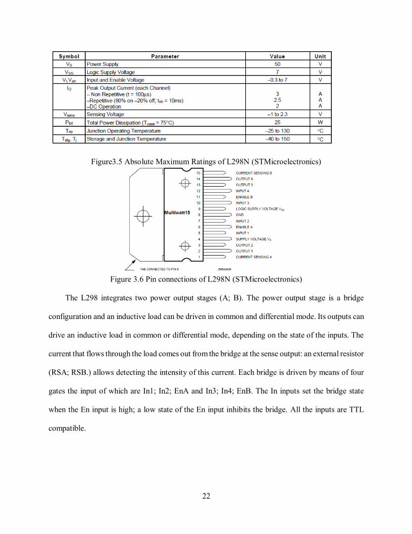
Figure3.5 Absolute Maximum Ratings of L298N (STMicroelectronics)

Figure 3.6 Pin connections of L298N (STMicroelectronics)

The L298 integrates two power output stages (A; B). The power output stage is a bridge

configuration and an inductive load can be driven in common and differential mode. Its outputs can

drive an inductive load in common or differential mode, depending on the state of the inputs. The

current that flows through the load comes out from the bridge at the sense output: an external resistor

(RSA; RSB.) allows detecting the intensity of this current. Each bridge is driven by means of four

gates the input of which are In1; In2; EnA and In3; In4; EnB. The In inputs set the bridge state

when the En input is high; a low state of the En input inhibits the bridge. All the inputs are TTL

compatible.

23

Figure 3.7 Schematic of the L298N Dual H Bridge DC Motor Driver (http://www.hotmcu.com/)

2. Stepper Motor Motion

A stepper motor is a brushless DC electric motor that contains a permanent magnet rotor and

a poly-phase coil stator. The DC electric motor contained in the stepper motor divides a full rotation

into numbers of equal steps. Then the motor’s position can be programmed to move forward or

backward at a fixed number of rotation. Also it can be programmed to change the direction by

changing the direction of applied magnetic field in the motor.

Figure 3.8 Schematic of the Stepper Motor- STP-MTR- 23055(D) (SureStep Stepping Motors)

24

Figure 3.9 Schematic of the EasyDriver (SchmalzHaus.com)

Each EasyDriver can drive up to about 750mA per phase of a bi-polar stepper motor. It defaults

to 8 step micro-stepping mode. (If the motor is 200 full steps per revolution, 1600 steps/rev would

be obtained using EasyDriver.) It is a chopper micro-stepping driver based on the Allegro

A3967 driver chip. It has a variable max current from about 150mA/phase to 750mA/phase. It can

take a maximum motor drive voltage of around 30V, and includes on-board 5V regulation, so only

one supply is necessary.

Closed-loop control principle

A closed-loop control system is also known as a feedback control system. Comparing to an

open loop system which has only forward path, a closed-loop control system has one or more

feedback paths or loops between its system input and system output. Here, “feedback” means one

or more branches of the system output return back to the system input to control the system itself.

Therefore, by monitoring the solar tracking system output and feeding back the system output to its

input, the whole control system could be accurately controlled.

The closed-loop control system that this article used were designed to automatically maintain

the solar panel facing the sun perpendicularly by comparing the desired solar panel position

25

(orienting the sun uprightly continuously) with the actual orientation of the solar panel. The

implementation of the process was generating an error signal that is the difference between the

system desired input and system output. The error was determined by the status of the photoelectric

sensors. The photoelectric sensors continually monitored the light intensity of the sun and fed a

digital signal based on the corresponding light intensity of the sun back to the controller as shown

below:

Figure 3.10 Closed-loop control principle diagram the solar panel tracking system

The motion controller in this research also chose the PID control loop principle. Because this

required a high level of determinism and was vital to the consistent operation, the control loop

typically closed on the board itself. Along with closing the control loop, the motion controller

managed supervisory control by monitoring the limits and emergency stops to ensure safe

operation. Directing each of these operations to occur on the board or in a real-time system ensures

the high reliability, determinism, stability, and safety necessary to create a working motion control

system. (Fundamentals of Motion Control, 2014)

Strategy of Third Objective

“Analyze the energy conversion efficiency gain.”

In order to certified that a solar tracking system produces more power over a longer time than

26

a stationary array with the same number of modules. The energy conversion efficiency of a latitude

fixed PV system and an automatic solar panel tracking system were compared by using an energy

consuming circuit as follow:

Figure 3.11 Energy conversion efficiency testing circuit

A 10-25 VDC, 3W warm white bulb was applied to the experiment to present the power

consuming. A voltmeter and an ampere meter were adopted to measure the voltage across the bulb

and the current passing through the bulb. The consuming power of the bulb was present by the

product of the reading value on the voltmeter and ampere meter.

The National Energy Strategy recommends a National commitment to greater efficiency in

every element of energy production and use. It suggested that greater energy efficiency can reduce

energy costs to consumers, enhance environmental quality, maintain and enhance our standard of

living, increase our freedom and energy security, and promote a strong economy. (National Energy

Strategy, Executive Summary, 1991/1992)

27

Figure 3.12 Schematic representation of an energy conversion device.

An energy conversion device was represented schematically in Figure 4-8. Energy supply and

demand at the macro-scale (United States and the world) were very much dependent on the balance

between energy input and output in the devices.

The efficiency of energy devices can be defined as a quantitative expression between energy

input and energy output as follow:

Device efficiency 𝜂 =𝑢𝑠𝑒𝑓𝑢𝑙 𝑒𝑛𝑒𝑟𝑔𝑦 𝑜𝑢𝑡𝑝𝑢𝑡

𝐸𝑛𝑒𝑟𝑔𝑦 𝑖𝑛𝑝𝑢𝑡=

𝑃

𝐸×𝐴𝐶 (3-1)

Here, “useful” depends on the purpose of the device. For the solar panel tracking system, the

useful energy output was the electrical power, and the energy input was the solar energy. P was the

useful energy output, E was the input light (in W/ m2) and AC was the surface area of the solar cell

(in m2).

In the research, a Daystar’s DS-05A solar meter measured the solar irradiance. After turning

the meter on and pointing the sensor at the light, the reading value of the light intensity was obtained

in Watt/m2.The data measurement were conducted in an indoor laboratory under the daylight lamps

and a sun simulator.

After applying the solar tracking system to regular PV system, to determine that if the energy

conversion system would increase in the PV system, the methodology of energy conversion

efficiency gain were defined and calculated as follow:

Gain (%) =𝑀𝑎𝑥𝑖𝑚𝑢𝑛 𝑒𝑛𝑒𝑟𝑔𝑦 𝑜𝑢𝑡𝑝𝑢𝑡(𝑆𝑜𝑙𝑎𝑟 𝑡𝑟𝑎𝑐𝑘𝑒𝑟)−𝐸𝑛𝑒𝑟𝑔𝑦 𝑜𝑢𝑡𝑝𝑢𝑡 (𝐿𝑎𝑡𝑖𝑡𝑢𝑑𝑒 𝑓𝑖𝑥𝑒𝑑 𝑃𝑎𝑛𝑒𝑙)

𝐸𝑛𝑒𝑟𝑔𝑦 𝑜𝑢𝑡𝑝𝑢𝑡 (𝐿𝑎𝑡𝑖𝑡𝑢𝑑𝑒 𝑓𝑖𝑥𝑒𝑑 𝑃𝑎𝑛𝑒𝑙) (3-2)

To directly describe the relationship between the efficiency gain through applying the solar

panel tracking system and the latitude angle of the solar panel, a Minitab software package was

Energy Conversion Device Energy output Energy input

28

utilized to implement the analysis. A fitted line plot was used to find the relationship between one

predictor (Latitude Angle of the Panel) and one response (Efficiency Gain (%)).

29

CHAPTER IV- FINDINGS

In order to complete this research, the following objectives needed to be completed.

1. Design an automatic solar tracking system using a LabVIEW and Arduino-based

controller

2. Designed a prototype of the system with solar panels, stepping motors, motor drives,

photosensitive sensors, Arduino, and LabVIEW controller.

3. Analyze the energy conversion efficiency gain.

This chapter presented an examination of these three objectives.

Discussion of Objective One

“Design an automatic solar tracking system using a LabVIEW and Arduino-based controller.”

System software environment design

The automatic solar tracking system was designed using a LabVIEW and Arduino-based

controller. The overview of the software for the automatic solar tracking system was as shown

below. It had three primary parts: Data acquisition, motor motion 1 (Latitude motion) and motor

motion 2 (Horizontal motion).

Figure 4.1 Software interface of the solar panel tracking system (LabVIEW)

30

Figure 4.2 Block diagram of the solar panel tracking system (LabVIEW)

System Mechanical Design

The mechanical 3D model of the solar tracking system was designed by SOLIDWORKS.

Then these 3D CAD files of the tracking system components designed by SOLIDWORKS were

printed through a 3D printer layer by layer. The mechanical structures of the solar panel system

were designed as shown in the figure below.

31

Figure 4.3 Dimension of the solar panel system

The structure of the solar panel tracking system consisted of several parts as shown in the

Figure above. The solar panel could be sustained and elevated or declined through a connecting

rod and a lead screw. The stepper drove the translation screw or lead screw back and forth.

Consequently, the lead screw nut was forced to move the connecting rod to elevate or decline the

solar panel. The software LabVIEW and Arduino controlled the stepper motor motion.

Figure 4.4 Latitude (Vertical) motion controller

As shown from the Figures above, the mechanical controller drove the solar panel up and

down on latitude. The system base supported the solar panel system. The DC motor was attached

to the base to control the horizontal rotation. Different seasons had different sun position. Sun

Solar

Panel

32

position could be varied based on different longitude, latitude and time zone of the locations. The

latitude motion controller assisted with the horizontal rotation controller could realize the function

of driving the solar panel focusing on the sun continuously.

Figure 4.5 Translation screw for the Latitude (Vertical) motion controller

A lead screw nut was used to as a linkage to connect the translation screw or lead screw with

the connecting rod. The lead screw was to transfer turning motion into linear motion. Even the

screw threads had larger frictional energy losses compared to other linkages because of the large

area of sliding contacted between the lead screw nut and the thread, it was more used for intermittent

usage in low power actuator and positioned mechanisms.

Figure 4.6 Lead Screw nut used to connect the transmission screw and connecting rod

33

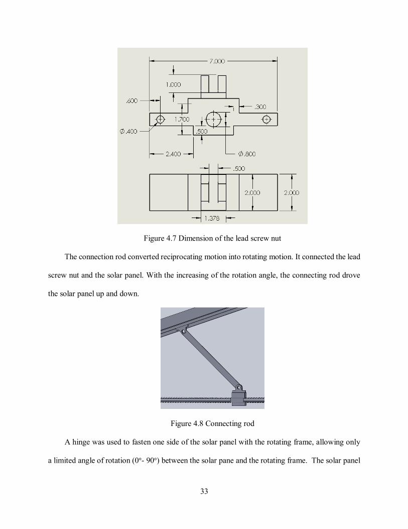
Figure 4.7 Dimension of the lead screw nut

The connection rod converted reciprocating motion into rotating motion. It connected the lead

screw nut and the solar panel. With the increasing of the rotation angle, the connecting rod drove

the solar panel up and down.

Figure 4.8 Connecting rod

A hinge was used to fasten one side of the solar panel with the rotating frame, allowing only

a limited angle of rotation (0°- 90°) between the solar pane and the rotating frame. The solar panel

34

and the rotating base were connected by the hinge rotate relative to each other about a fixed axis of

rotation.

Figure 4.9 Hinge used to connect the solar panel with the rotating base.

Figure 4.10 Horizontal (Rotating) motion controller

35

Figure 4.11 Dimension of the horizontal motion controller

The horizontal (Rotating) motion controller consisted of a rotating frame and the supporting

base with a pair of internal gears. The outer gear was attached to the rotating frame and the inner

gear was attached to the stationary base.

Figure 4.12 Base of the solar tracking system

36

Figure 4.13 Dimension of the base of the solar pane tracking system

In the solar panel system, an inner gear was used for rotating the DC motor to function the

horizontal movement. Inner gears were spur gears turned "inside out." In other words, the teeth

were cut into the inside diameter while the outside diameter is kept smooth. This design allowed

for the DC motor to rotate the inner gear under the control of the LabVIEW and Arduino program

to rotate the outer gear in further. The attached outer gear then drove the rotating frame rotating.

37

Figure 4.14 Internal gear (inner one) of the horizontal controller and its dimension

Figure 4.15 Internal gear (outer one) of the horizontal controller and its dimension

Discussion of Objective Two

“Design a prototype of the system with solar panels, stepping motors, motor drives, photosensitive

sensors, Arduino, and LabVIEW controller.”

Data Acquisition

The function of data acquisition section was to acquire data through the photoelectric sensors.

Photoelectric sensors were normally made up of a LED, a receiver (phototransistor), a signal

38

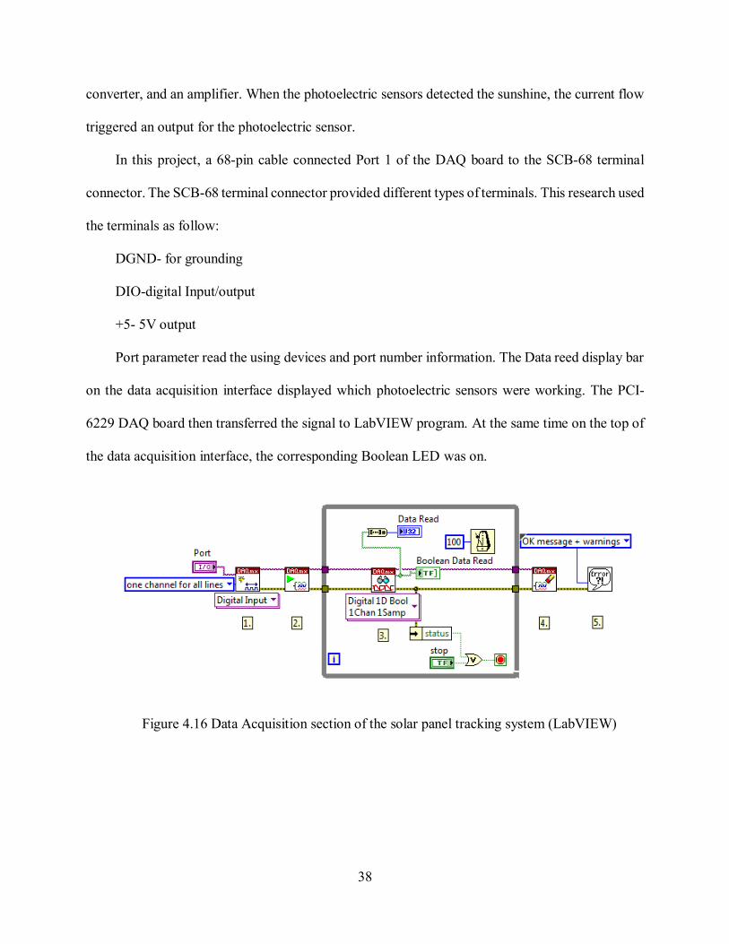
converter, and an amplifier. When the photoelectric sensors detected the sunshine, the current flow

triggered an output for the photoelectric sensor.

In this project, a 68-pin cable connected Port 1 of the DAQ board to the SCB-68 terminal

connector. The SCB-68 terminal connector provided different types of terminals. This research used

the terminals as follow:

DGND- for grounding

DIO-digital Input/output

+5- 5V output

Port parameter read the using devices and port number information. The Data reed display bar

on the data acquisition interface displayed which photoelectric sensors were working. The PCI-

6229 DAQ board then transferred the signal to LabVIEW program. At the same time on the top of

the data acquisition interface, the corresponding Boolean LED was on.

Figure 4.16 Data Acquisition section of the solar panel tracking system (LabVIEW)

39

Figure 4.17 Sensor experiments of the solar panel tracking system

As shown in Figure 4.17, when tested using a flash light, the photoelectric sensors would

operate as shown on the software interface. The Boolean indicator would be on. Also, Channel

Parameters section would display which device and port is working. Data Read section would

display which photoelectric sensor was working. At the same time, an oscilloscope would detect a

voltage waveform changing on the photoelectric sensor.

Figure 4.18 Data Acquisition interface of the solar panel tracking system (LabVIEW) (a)

Figure 4.19 Data Acquisition interface of the solar panel tracking system (LabVIEW) (b)

40

Figure 4.20 Data Acquisition interface of the solar panel tracking system (LabVIEW) (c)

Figure 4.21 Data Acquisition interface of the solar panel tracking system (LabVIEW) (d)

Motor Motion

1. DC Motor

First connect each motor to the A and B connections on the L298N module. Next, connect the

power supply - the positive power supply sign on the module and negative/GND. In this system the

power supply as up to 12V so the 12V jumper was left and 5V was available on the module. Also

connect Arduino GND to pin 5 on the module as well to complete the circuit.

Then six digital output pins on the Arduino were connected to the L298N Dual H Bridge DC

Motor Driver, two of which needed to be PWM (pulse-width modulation) pins. PWM pins were

denoted by the tilde ("~") next to the pin number as shown below:

41

Figure 4.22 Digital (PWM) pins on Arduino

Finally, connect the Arduino digital output pins to the driver module. Digital pins D6 and D7,

D7 were connected to pins IN1, IN2 respectively. Then remove the EnA jumper and connect D5 to

it. The wring diagram of the Arduino and the L298N Dual H Bridge DC Motor Driver was shown

as follow:

Figure 4.23 Wring diagram of the Arduino and the L298N Dual H Bridge DC Motor Driver

2. Stepper Motor Motion

The stepper direction was controlled by sending a HIGH or LOW signal to the drive for the

motor. However the motors did not be turned on until a HIGH was set to the enable pin. And they

could be turned off with a LOW to the same pin(s).

42

Connect the motor's four wires to the Easy Driver (note the proper coil connections), connect

a power supply of 12V to the Power In pins, and connect the Arduino's GND, pin 2 and pin 3 to the

Easy Driver as follow.

Figure 4.24 Wring diagram of the Arduino and the L298N Dual H Bridge DC Motor Driver

The stepper motor motion section of the solar panel tracking system was designed as shown

in Figure 4.25. On the front panel, the photoelectric sensors detected the sun position. Based on the

sun position and the closed-loop control method, motor 1 and 2 moved forward to the desired

position. When a motor was running, the corresponding Boolean indicator was turned on as shown

on the software interface. For emergency, users could click ‘stop’ button on the software interface

to halt the motor.

On the block diagram, the program consisted of all the cases detected by photoelectric sensors.

Different Case Structures combines with While Loops were designed to implement the functions

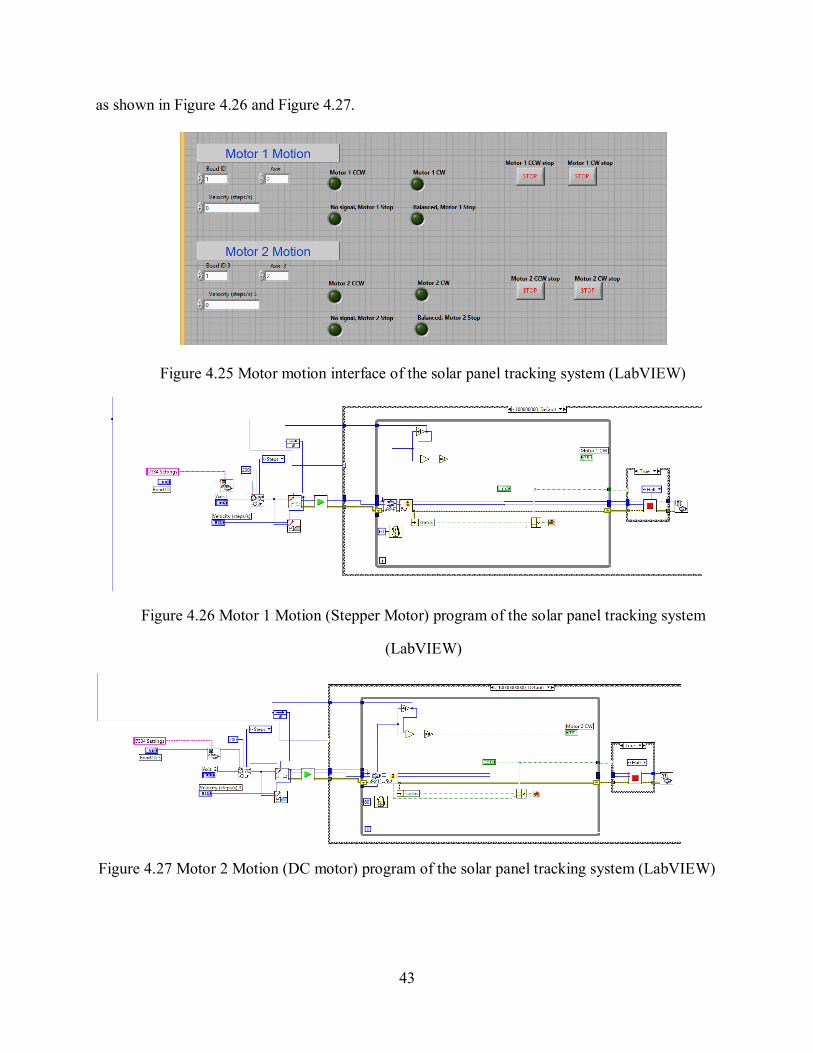
43

as shown in Figure 4.26 and Figure 4.27.

Figure 4.25 Motor motion interface of the solar panel tracking system (LabVIEW)

Figure 4.26 Motor 1 Motion (Stepper Motor) program of the solar panel tracking system

(LabVIEW)

Figure 4.27 Motor 2 Motion (DC motor) program of the solar panel tracking system (LabVIEW)

44

Discussion of Objective Three

“Analyze the energy conversion efficiency gain.”

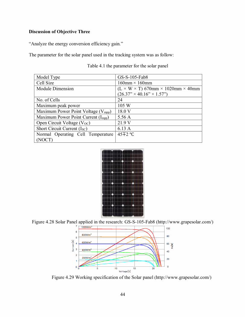
The parameter for the solar panel used in the tracking system was as follow:

Table 4.1 the parameter for the solar panel

Model Type GS-S-105-Fab8

Cell Size 160mm × 160mm

Module Dimension (L × W × T) 670mm × 1020mm × 40mm

(26.37” × 40.16” × 1.57”)

No. of Cells 24

Maximum peak power 105 W

Maximum Power Point Voltage (Vmpp) 18.0 V

Maximum Power Point Current (Impp) 5.56 A

Open Circuit Voltage (VOC) 21.9 V

Short Circuit Current (ISC) 6.13 A

Normal Operating Cell Temperature

(NOCT)

45∓2 ℃

Figure 4.28 Solar Panel applied in the research: GS-S-105-Fab8 (http://www.grapesolar.com/)

Figure 4.29 Working specification of the Solar panel (http://www.grapesolar.com/)

45

To present the power consuming, a DC bulb was applied to the experiment. A voltmeter and

an ampere meter were adopted to measure the voltage across the bulb and the current passing

through the bulb. The consuming power of the bulb was present by the product of the reading on

the voltmeter and ampere meter.

Daylight lamps

The data measurement was conducted in an indoor laboratory under daylight lamps. Also the

position of the solar panel was fixed to reduce the disturbing signals and measurement errors. The

output voltage and the output current were measured as shown in the table below.

Table 4.2 Data measurement of the output voltage and the output current (daylight lamps)

Latitude

Angle/° Output Current/mA Output Voltage/V

Average

Output

Current/ mA

Average Output

Voltage/V

90 4.20 4.14 4.22 2.01 2.01 2.01 4.187 2.010

85 4.41 4.31 4.39 2.01 2.01 2.01 4.370 2.010

80 4.68 4.57 4.65 2.01 2.01 2.01 4.633 2.010

75 5.23 5.01 5.17 2.01 2.01 2.01 5.137 2.010

70 5.91 5.61 5.92 2.02 2.01 2.02 5.813 2.017

65 6.57 6.20 6.52 2.02 2.02 2.02 6.430 2.020

60 7.09 7.11 7.05 2.02 2.02 2.02 7.083 2.020

55 7.60 7.55 7.60 2.02 2.02 2.02 7.583 2.020

50 8.00 7.98 8.10 2.02 2.02 2.02 8.027 2.020

45 8.53 8.45 8.47 2.02 2.02 2.02 8.483 2.020

40 9.02 8.95 8.99 2.03 2.02 2.03 8.987 2.027

35 9.56 9.45 9.49 2.03 2.03 2.03 9.500 2.030

30 10.02 10.07 9.95 2.03 2.03 2.03 10.013 2.030

25 10.37 14.45 10.50 2.03 2.03 2.03 11.773 2.030

20 10.76 10.93 10.93 2.03 2.03 2.02 10.873 2.027

15 11.17 11.18 11.18 2.03 2.03 2.03 11.177 2.030

10 11.41 11.47 11.44 2.03 2.03 2.03 11.440 2.030

5 11.57 11.60 11.63 2.03 2.03 2.03 11.600 2.030

0 11.59 11.59 11.63 2.03 2.03 2.03 11.603 2.030

Three group measurements were conducted in the experiment and the data were shown in the

46

output current and the output voltage columns. The unit for the Current was Ampere and the Voltage

was Volt. The Unit for Power consuming in the circuit was Watt. The unit for the input light intensity

is W/ m2.

In this experiment, AC = Cell Size=24 × (160 × 160 -2 × 1.52) mm2=

614,292mm2=0.614292 m2 (4-1)

Based on the measurement, the solar system maximum efficiency occurs when the Latitude

Angle is 0 degree, where the maximum device efficiency is:

𝜂𝑀𝑎𝑥 =𝑢𝑠𝑒𝑓𝑢𝑙 𝑒𝑛𝑒𝑟𝑔𝑦 𝑜𝑢𝑡𝑝𝑢𝑡

𝐸𝑛𝑒𝑟𝑔𝑦 𝑖𝑛𝑝𝑢𝑡=

𝑃

𝐸×𝐴𝐶=

11.603𝑚𝐴×2.03𝑉

2Watt/ 𝑚2×0.614292𝑚2=1.917174% (4-2)

While on the Latitude-fixed solar panel system, the energy conversion efficiency is varied.

System only reached its maximum output when the latitude angle is 0. However, since the solar

panel is fixed on Latitude, the energy conversion system could only reach the maximum device

efficiency momently as the sum position moves continuously.

The minimum device efficiency happened when the latitude angle reached 90 degree on the

moment of sunset.

𝜂𝑀𝑖𝑛 =𝑢𝑠𝑒𝑓𝑢𝑙 𝑒𝑛𝑒𝑟𝑔𝑦 𝑜𝑢𝑡𝑝𝑢𝑡

𝐸𝑛𝑒𝑟𝑔𝑦 𝑖𝑛𝑝𝑢𝑡=

𝑃

𝐸×𝐴𝐶=

4.187𝑚𝐴×2.010𝑉

2Watt/ 𝑚2×0.614292𝑚2=0.6850% (4-3)

From the measurement, Gain (%) = 𝑃𝑚𝑎𝑥−𝑃𝐿

𝑃𝑚𝑎𝑥𝐸 =

𝑀𝑎𝑥{𝑈𝐼}−𝑈𝐼

𝑀𝑎𝑥{𝑈𝐼} (4-4)

Where, U stood for the average output voltage, I was the average output current.

47

Table 4.3 Data calculation based on the output voltage and the output current. (Daylight lamp)

Latitude Angle

of the Panel/°

Average

Output

Current/ mA

Average Output

Voltage/V

Efficiency

Gain (%)

90 4.187 2.010 726.84%

85 4.370 2.010 679.40%

80 4.633 2.010 617.83%

75 5.137 2.010 517.70%

70 5.813 2.017 410.43%

65 6.430 2.020 331.94%

60 7.083 2.020 263.69%

55 7.583 2.020 219.40%

50 8.027 2.020 184.74%

45 8.483 2.020 152.83%

40 8.987 2.027 120.47%

35 9.500 2.030 91.24%

30 10.013 2.030 65.44%

25 10.440 2.030 45.92%

20 10.873 2.027 28.30%

15 11.177 2.030 15.73%

10 11.440 2.030 5.88%

5 11.600 2.030 0.12%

0 11.603 2.030 0.00%

Figure 4.30 Energy conversion efficiency gain by applied Solar panel tracking system VS.

9080706050403020100

800.00%

700.00%

600.00%

500.00%

400.00%

300.00%

200.00%

100.00%

0.00%

S 0.842678

R-Sq 88.7%

R-Sq(adj) 88.0%

Latitude Angle of the Panel

Eff

icie

ncy G

ain

(%)

Fitted Line PlotEfficiency Gain(%) = - 1.313 + 0.08155 Latitude Angle of the Panel

48

Latitude Angle of the solar panel (Calculated in Minitab).

A fitted line plot was used to find the relationship between one predictor (Latitude Angle of

the Panel) and one response (Efficiency Gain (%)). The response variables are displayed on the y-

axis and the predictor variable are displayed on the x-axis. A linear model is chosen to best describe

the relationship between them. The relationship between the efficiency gain and the latitude angle

of the panel comparing the solar panel tracking system and the latitude fixed PV system can be

indicated by a mathematic expression:

Efficiency Gain (%) = -1.313 + 0.08155 Latitude Angle of the Panel. (4-5)

Sun Simulator

Same as the measurement conducted under the daylight lamp, the data measurement in this

experiment was conducted in an indoor laboratory under a sun simulator. Also the position of the

solar panel was fixed to reduce the disturbing signals and measurement errors. The output voltage

and the output current were measured as shown in the table below.

49

Table 4.4 Data measurement of the output voltage and the output current (sun simulator)

Three group measurements were conducted in the experiment and the data were shown in

the output current and the output voltage columns. In this experiment,

AC = Cell Size=24 × (160 × 160 -2 × 1.52) = 614,292mm2=0.614292 m2 (4-6)

Based on the measurement, the solar system maximum efficiency occurs when the Latitude

Angle is 0 degree, where the maximum device efficiency was:

𝜂𝑀𝑎𝑥 =𝑢𝑠𝑒𝑓𝑢𝑙 𝑒𝑛𝑒𝑟𝑔𝑦 𝑜𝑢𝑡𝑝𝑢𝑡

𝐸𝑛𝑒𝑟𝑔𝑦 𝑖𝑛𝑝𝑢𝑡=

𝑃

𝐸×𝐴𝐶=

198.833𝑚𝐴×2.030𝑉

35Watt/ 𝑚2×0.614292𝑚2=1.8877% (4-7)

Latitude Angle/°

Output Current/mA Output Voltage/V Average Output

Current/ mA

Average Output

Voltage/V

0 198.00 198.50 200.00 2.03 2.03 2.03 198.833 2.030

5 192.60 193.30 195.00 2.03 2.03 2.03 193.633 2.030

10 186.20 186.20 188.00 2.03 2.03 2.03 186.800 2.030

15 178.50 179.20 180.70 2.03 2.02 2.02 179.467 2.023

20 170.80 170.00 172.70 2.02 2.01 2.02 171.167 2.017

25 160.70 161.00 164.20 2.02 2.01 2.02 161.967 2.017

30 150.00 152.00 154.00 2.03 2.01 2.02 152.000 2.020

35 140.70 142.50 142.80 2.02 2.00 2.02 142.000 2.013

40 130.70 132.30 131.90 2.02 2.00 2.01 131.633 2.010

45 120.90 121.40 120.90 2.03 2.00 2.01 121.067 2.013

50 109.40 108.90 109.90 2.03 1.99 2.01 109.400 2.010

55 97.60 99.00 98.00 2.03 1.98 2.00 98.200 2.003

60 85.50 86.20 86.80 2.02 1.97 1.98 86.167 1.990

65 73.70 75.50 76.60 2.02 1.96 1.99 75.267 1.990

70 63.50 65.30 65.10 2.01 1.98 1.99 64.633 1.993

75 54.20 54.40 54.10 1.99 1.97 1.98 54.233 1.980

80 39.70 43.60 43.50 1.98 1.95 1.97 42.267 1.967

85 31.70 35.00 34.90 1.96 1.94 1.95 33.867 1.950

90 29.10 30.30 30.50 1.95 1.93 1.93 29.967 1.937

50

Table 4.5 Data calculation based on the output voltage and the output current (sun simulator)

Latitude Angle/°

Average Output

Current/ mA

Average Output

Voltage/V

Output Power/

Watt Gain (%)

90 198.833 2.030 0.404 2233.50%

85 193.633 2.030 0.393 2165.28%

80 186.800 2.030 0.379 2075.63%

75 179.467 2.023 0.363 1971.69%

70 171.167 2.017 0.345 1855.78%

65 161.967 2.017 0.327 1735.87%

60 152.000 2.020 0.307 1609.25%

55 142.000 2.013 0.286 1472.59%

50 131.633 2.010 0.265 1334.86%

45 121.067 2.013 0.244 1200.21%

40 109.400 2.010 0.220 1046.05%

35 98.200 2.003 0.197 896.33%

30 86.167 1.990 0.171 733.11%

25 75.267 1.990 0.150 592.93%

20 64.633 1.993 0.129 457.56%

15 54.233 1.980 0.107 318.91%

10 42.267 1.967 0.083 162.14%

5 33.867 1.950 0.066 51.73%

0 29.967 1.937 0.058 0.00% The minimum device efficiency happened when the latitude angle reached 90 degree on the

moment of sunset.

𝜂𝑀𝑖𝑛 =𝑢𝑠𝑒𝑓𝑢𝑙 𝑒𝑛𝑒𝑟𝑔𝑦 𝑜𝑢𝑡𝑝𝑢𝑡

𝐸𝑛𝑒𝑟𝑔𝑦 𝑖𝑛𝑝𝑢𝑡=

𝑃

𝐸×𝐴𝐶=

29.967𝑚𝐴×1.937𝑉

35Watt/ 𝑚2×0.614292𝑚2=0.269979% (4-8)

From the measurement, Gain (%) = 𝑃𝑚𝑎𝑥−𝑃𝐿

𝑃𝑚𝑎𝑥𝐸 =

𝑀𝑎𝑥{𝑈𝐼}−𝑈𝐼

𝑀𝑎𝑥{𝑈𝐼} (4-9)

51

Figure 4.31 the energy conversion efficiency gain by applied Solar panel tracking system VS.

Latitude Angle of the solar panel (Calculated in Minitab).

A fitted line plot was used to find the relationship between one predictor (Latitude Angle of

the Panel) and one response (Efficiency Gain (%)). The response variables are displayed on the y-

axis and the predictor variable are displayed on the x-axis. A linear model is chosen to best describe

the relationship between them. The relationship between the efficiency gain and the latitude angle

of the panel comparing the solar panel tracking system and the latitude fixed PV system can be

indicated by a mathematic expression:

Efficiency Gain (%) = -0.4593 + 0.26656 Latitude Angle of the Panel. (4-10)

Two different results generated by two different light sources. In this study, the energy

conversion efficiency of the solar panel is relatively low comparing to the maximum efficiency of

12% announced by DOE. However, the energy conversion gain (%) had been improved

significantly. When applying daylight as the light resource, the energy conversion gain (%) that

increased through the solar panel tracking system can be as high as 726.84% compared to latitude

9080706050403020100

2500.00%

2000.00%

1500.00%

1000.00%

500.00%

0.00%

S 0.500677

R-Sq 99.6%

R-Sq(adj) 99.6%

Latitude Angle of the Panel

Co

nvers

ion

Eff

icie

ncy G

ain

(%)

Fitted Line PlotConversion Efficiency Gain(%) = - 0.4593 + 0.2665 Latitude Angle of the Panel

52

tilt PV systems. The average energy conversion gain is 235.68%. Thus the solar tracking system

enhanced the solar energy conversion efficiency.

The results had a notable difference of the energy conversion efficiency gain (%) between the

daylight lamp and the sun simulator. Some possible reasons could be: The layouts of the daylight

lamps in the day are divergent; the incident rays that reached the solar panel were not as parallel.

This would affect the energy conversion efficiency gain to some extent.

Another experiment which conducted under the sun simulator caused apparently higher energy

conversion efficiency gain than daylight lamps. The maximum energy conversion efficiency gain

was 2233.50%. The average energy conversion efficiency gain was 1153.34%. Some likely reasons

could be: The lights of sun simulator are focus and parallel; the incident rays that reached the solar

panel were also parallel. In this situation, the sun simulator has the characteristics of the actual sun.

Thus, the result when applying a sun simulator is more reliable and convincible.

53

CHAPTER V- CONCLUSION, RECOMMENDATIONS, AND FUTURE RESEARCH

Conclusion

The energy conversion efficiency of the solar tracking system has been evaluated to determine

the feasibility of a solar panel tracking system. The main reason to use a solar panel tracking system

is to reduce the cost of the energy to some extent. A tracker produces more power than a stationary

array or latitude tilt fixed PV system with the same number of modules. This additional energy

conversion output or “gain” can be quantified as a percentage of the output of the stationary array.

The gain varies significantly with latitude and the orientation of a stationary installation in the same

location. In general, a solar panel tracking system adds most to output during the hours when a

stationary array produces the least power.

This study could be a systematic foundation for future works to continue to build a solar panel

system used for industries. The DC motor and L298N Dual H Bridge DC Motor Driver, the Stepper

motor and EasyDriver Stepper Motor Driver V4.4 have been tested and certified that they could be

equipped on the solar tracking system to drive a solar panel which dimension is 160mm × 160mm.

As indicated in the tables and graphs, by applying a solar panel tracking system to PV system,

the energy conversion efficiency is increased significantly. Two different results generated by two

different light sources indicates the relationship between one predictor (Latitude Angle of the Panel)

and one response (Efficiency Gain (%)). The energy conversion gain (%) has been improved

notably both when applying daylight as the light resource and a sun simulator as the light resource.

The poor conversion efficiency associated with the Latitude fixed PV systems leads one to the

conclusion that the development of a solar panel tracking system will be practical and significant.

54

Recommendations

Chapter IV concludes that the development of a solar panel tracking system will be practical

and significant. The energy conversion efficiency can be increased notably by applying a automatic

solar tracking system to PV system.

1. It is recommended that the engineers and researchers develop more detailed experiments

with a variety of motors and the corresponding drivers.

2. Given that this study provides a variety of design for conducting a research of a LabVIEW

and Arduino-based solar panel tracking system. The structure of the solar panel tracking

system is feasible. It is suggested that researchers could conduct comparisons with other

structures and the structure that used in this research.

3. It is suggested that the researchers to develop some type of experiments to study of the

system energy dissipation through system friction and motor rotations.

Future Research

This study could be a systematic foundation for future works to continue to build upon.

Currently the energy conversion efficiency of the solar tracking system has been evaluated to

determine the feasibility of a solar panel tracking system. As part of future research, more real-time

data could be obtained and analyzed after the real solar tracker are built.

Future research should be conducted focus on finding a methodology for the function of anti-

interference. A practical solar panel tracking system should be able to detect the weather condition

and take actions correspondingly.

Future research should also be conducted into the working conditions outdoor. The solar panel

tracking system should perform normally under the extreme weather such as heavy rain and snow.

Researchers would look to apply more advanced materials to prevent metal parts, such as the shaft

55

in the solar tracking system, from rusting and the subsequent problems that might damage the

system caused by rusting.

Finally, future research is needed into replacing the LabVIEW module with Arduino module

including corresponding software and hardware. As Arduino is getting more popular and cheap, the

software and hardware developer will benefit from economizing funds and its compatibility.

56

REFERENCES

Alt, M. (2015, April 1). America's Top Solar Cities. Retrieved April 24, 2015, from

http://www.huffingtonpost.com/margie-alt/americas-top-solar-cities_b_6979304.html

BP Statistical Review of World Energy 2014. (2014, June). Retrieved February 9, 2015, from

http://www.commodities-now.com/reports/power-and-energy/16971-bp-statistical-

review-of-world-energy-2014.html

Building an NI Motion Control System. (2013, November 27). Retrieved February 8, 2015, from

http://www.ni.com/white-paper/12127/en/

Chapin, D. M., Fuller, C. S., Pearson, G. L. (1954). Applied Physics, 25, 676.

Characteristics of Mediterranean Climates. (1973.). Retrieved March 11, 2015, from

http://gimcw.org/climate/characteristics.cfm

Dolara, A., Grimaccia, F., Leva, S., Mussetta, M., Faranda, R., & Gualdoni, M. (2012).

Performance Analysis of a Single-Axis Tracking PV System. IEEE Journal of

Photovoltaics, 2(4), 524-531.

Dunlop, J. (2010). Photovoltaic systems (2nd Ed.). Orland Park, Ill.: American Technical.

Early Solar History. (1999). Retrieved February 9, 2015, from

http://solarcellcentral.com/history_page.html

Eke, R., & Senturk, A. (2012). Performance comparison of a double-axis sun tracking versus

fixed PV system. Solar Energy, 86(9), 2665-2672.

Fox, C. (2014, April 14). The 20 Best Cities for Solar Power as America Prepares for an Energy

'Revolution' Retrieved April 20, 2015, from

http://www.huffingtonpost.com/2014/04/17/best-cities-solar-power_n_5162615.html

Fritts,C.E. (1883). On a new form of selenium photocell. American Journal Science, 26,465.

57

Fundamentals of Motion Control. (2014, December 9). Retrieved February 8, 2015, from

http://www.ni.com/white-paper/3367/en/

History of Solar Energy in California - Go Solar California. (1999). Retrieved February 9, 2015,

from http://www.gosolarcalifornia.ca.gov/about/gosolar/california.php

History of Solar Energy. (2012). Retrieved February 9, 2015, from

http://exploringgreentechnology.com/solar-energy/history-of-solar-energy/

Horace de Saussure and his hot boxes of the 1700's. (2004). Retrieved February 6, 2015, from

http://solarcooking.org/saussure.htm

Lee, C.Y., Chou, P.C., Chiang, C.M., Lin, C.F., 2009. Sun tracking systems: a review. Sensors 9,

3875–3890

Lynn, P. (2010). Electricity from sunlight: An introduction to photovoltaics. Chicester: Wiley-

Blackwell (an imprint of John Wiley & Sons).

Maish, A. B. (1990, May 21-25). Performance of a self-aligning solar array tracking controller.

In Proceedings of the IEEE Photovoltaic Specialists Conference, Kissimimee, FL, USA.

McFee, R.H. (1975). Power collection reduction by mirror surface non flatness and tracking

error for a central receiver solar power system. Appl. Opt., 14, 1493-1502.

One Platform, Infinite Possibilities. (1999). Retrieved April 24, 2015, from

http://www.ni.com/labview/why/

United States. (1991). National energy strategy: Executive summary. Washington, D.C: U.S.

Dept. of Energy.

Semma, R. P.; Imamura, M. S. (1980). Sun tracking controller for multi-kW photovoltaic

concentrator system. In Proceedings of the 3rd International Photovoltaic Sol Energy

Conference, Cannes, France, Oct. 27-31.

58

Sherwood, L. (2012). U.S. Solar Market Trends 2011. Interstate Renewable Energy Council

(IREC) annual report

Smith, W. (1873). Effect of Light on Selenium during the Passage of an Electric Current. Nature,

1(173), 303-303.

Tomaszewski, P. (1998). Professor Jan Czochralski (1885-1953) AND HIS CONTRIBUTION

TO THE ART AND SCIENCE OF CRYSTAL GROWTH. American Crystallographic

Association, 27(2).

TRENDS in Photovoltaic Applications - 2013. (2013). Retrieved February 9, 2015, from

http://www.iea-

vps.org/fileadmin/dam/public/report/statistics/FINAL_TRENDS_v1.02.pdf

Zamostny, D. (2011, June 17). Solar history: Alexandre Edmond Becquerellar - Solar Energy

World. Retrieved February 6, 2015, from

http://www.solarenergyworld.com/2011/06/17/solar-history-alexandre-edmond-

becquerel/

59

APPENDIX

60

Fig

ure

4.1

Soft

war

e in

terf

ace

of

the

sola

r pan

el t

rack

ing s

yst

em (

Lab

VIE

W)

61

Fig

ure

4.2

Blo

ck d

iagra

m o

f th

e so

lar

pan

el t

rack

ing s

yst

em (

Lab

VIE

W)

62

Fig

ure

4.7

Dim

ensi

on o

f th

e le

ad s

crew

nut

63

Fig

ure

4.1

1 D

imen

sion o

f th

e hori

zonta

l m

oti

on c

ontr

oll

er

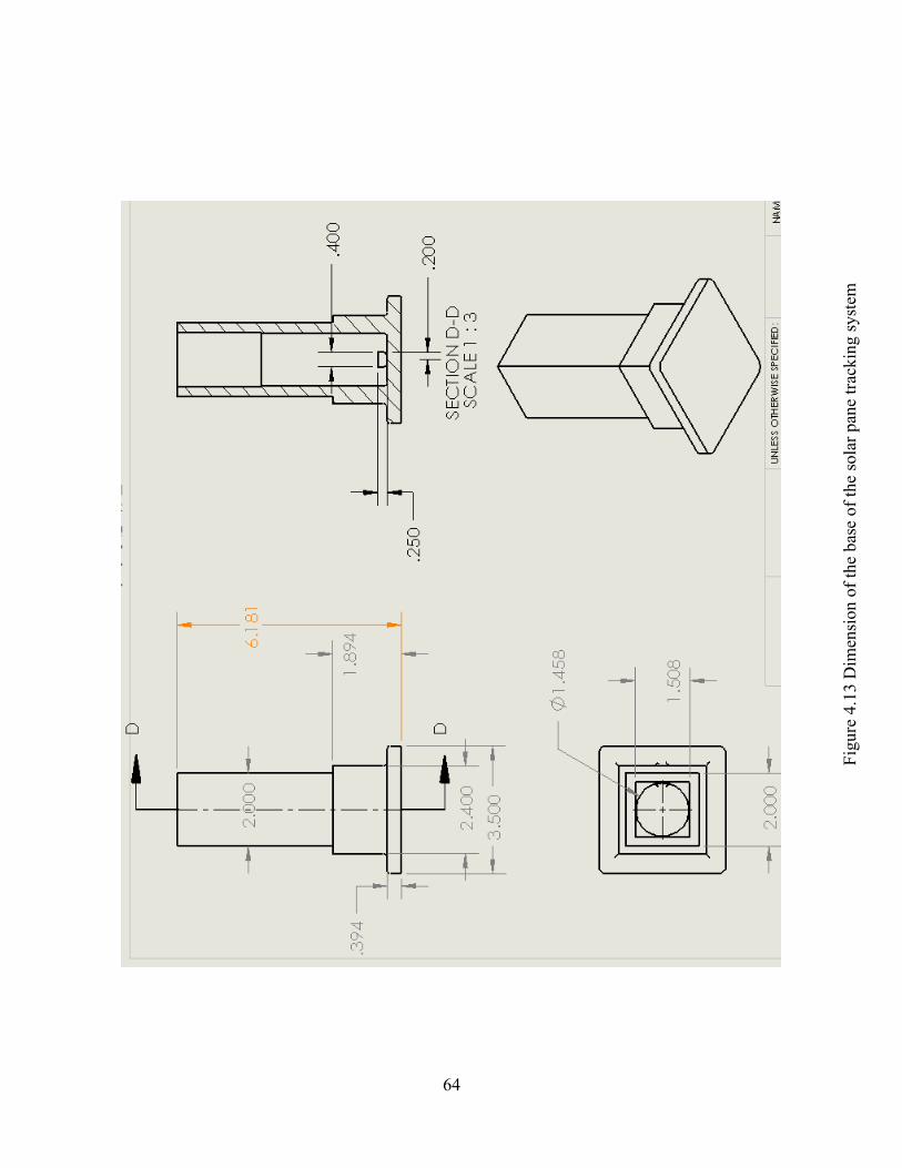
64

Fig

ure

4.1

3 D

imen

sion o

f th

e bas

e of

the

sola

r pan

e tr

ackin

g s

yst

em

65

Fig

ure

4.1

4 I

nte

rnal

gea

r (i

nner

one)

of

the

hori

zonta

l co

ntr

oll

er a

nd i

ts d

imen

sion

66

Fig

ure

4.1

5 I

nte

rnal

gea

r (o

ute

r one)

of

the

hori

zonta

l co

ntr

oll

er a

nd i

ts d

imen

sion

67

Fig

ure

4.1

6 D

ata

Acq

uis

itio

n s

ecti

on o

f th

e so

lar

pan

el (

Lab

VIE

W)

trac

kin

g s

yst

em (

Lab

VIE

W)

68

Fig

ure

4.2

3 W

ring d

iagra

ms

of

the

Ard

uin

o a

nd t

he

L298N

Dual

H B

ridge

DC

Moto

r D

river

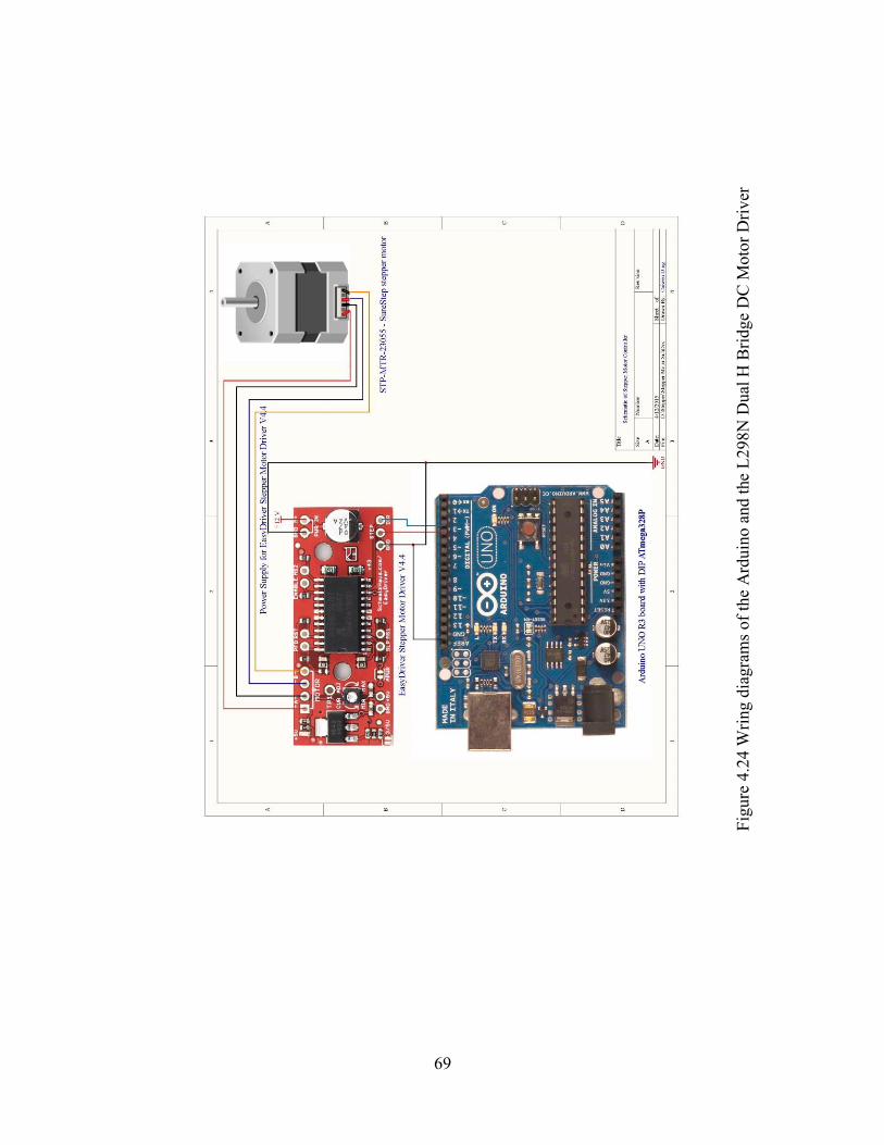
69

Fig

ure

4.2

4 W

ring d

iagra

ms

of

the

Ard

uin

o a

nd t

he

L298N

Dual

H B

ridge

DC

Moto

r D

river

70

Fig

ure

4.2

6 M

oto

r 1 M

oti

on p

rogra

m o

f th

e so

lar

pan

el t

rack

ing s

yst

em (

Lab

VIE

W)

71

Fig

ure

4.2

7 M

oto

r 2

Moti

on p

rogra

m o

f th

e so

lar

pan

el t

rack

ing s

yst

em (

Lab

VIE

W)