Embed Size (px)
Citation preview

Design and Analysis of a Soft Prismatic Joint
by
Amelia Tepper Servi
SUBMITTED TO THE DEPARTMENT OF MECHANICAL ENGINEERING IN PARTIALFULFILLMENT OF THE REQUIREMENTS FOR THE DEGREE OF
BACHELORS OF SCIENCE IN MECHANICAL ENGINEERINGAT THE
MASSACHUSETTS INSTITUTE OF TECHNOLOGY
JUNE 2010
@2010 Amelia Tepper Servi. All rights reserved.
OF TECHNOLOGY
JUN 3 0 2010
LIBRARI ES
ARCHNESThe author hereby grants to MIT permission to reproduce
and to distribute publicly paper and electroniccopies of this thesis document in whole or in partin any medium now known or hereafter created.
AuthorD rtment echanical Engineering
X/ M May 10 th010
Certified byMartin L. Culpepper
Associate Professor of Mechanical EngineeringThesis Supervisor
John H. Lienhard Vofessor of Mechanical Engineering
Chairman, Undergraduate Thesis Committee
Accepted by

Design and Analysis of a Soft Prismatic Joint
by
Amelia Tepper Servi
Submitted to the Department of Mechanical Engineeringon May 10, 2010 in partial fulfillment of the
Requirements for the Degree of Bachelor of Science inMechanical Engineering
ABSTRACT
This thesis documents the design and analysis of a soft prismatic joint for use in soft robotics.While this joint can be utilized in any soft robot, its immediate application is for Squishbot, asoft robot developed for the DARPA Chembot challenge. For the Squishbot application, the jointmust fit within a cylindrical envelope 4cm long and 1cm in diameter, compress 1.2cm axiallywithout buckling, and be soft such that it can undergo large deformations without plasticallydeforming. After considering a wide range of design concepts, a screw design was chosen. Thisdesign concept was selected because it has a high axial to bending compliance ratio and does notexpand radially when compressed axially. A model was developed to describe this design as afunction of its design parameters. A metric was also developed to predict based on a single-cellsample whether a full-scale model would be able to fulfill the design requirements. The modelwas validated with respect to the parameter of blade thickness by testing 3D printed, TangoPluscell-pairs. The results show that the model is correct to within a factor of three over bladethickness but needs further modifications to better predict trends in joint behavior. The designstill needs to be tested over other parameters such as cell height. Preliminary work was alsoconducted on designing a locking mechanism for the joint, but more work is needed in this area.Overall, the design presented in this thesis fulfills the project's design requirements and themodel that was developed describes the joint's behavior to first order.
Thesis Supervisor: Prof. Martin CulpepperTitle: Associate Professor of Mechanical Engineering

ACKNOWLEDGEMENTS
I would like to thank Prof. Martin Culpepper for his direction throughout this project and for hisacademic advising in general. He has been instrumental in encouraging me to pursue futurework in mechanical design.
I would also like to thank Maria Telleria for guiding me during this project. She has been a greatteacher and role model.
I would like to thank Nadia Cheng and Alex Slocum Jr. for answering my questions and keepingthe 3D printer in working order.
Finally, I would like to thank Matt Ritter, Nimrod Gileadi, Ben Derrett, Raju Krishnamoorthyand Arathi Ramachandaram for reading this thesis and giving me valuable feedback.
This material is based upon work supported by, or in part by, the U. S. Army ResearchLaboratory and the U. S. Army Research Office under contract/grant number W91 lNF-08-C-0055.his work was supported in part by the U.S. Defense Advanced Research Projects Agency(DARPA) under the Chemical Robots Program.
Additional funding was provided by the MIT UROP office.

Table of Contents
ABSTRACT.................................................................................................................................... 2ACKNOW LEDGEM EN TS...................................................................................................... 3Table of Contents ............................................................................................................................ 4List of Figures ................................................................................................................................. 5List of Tables................................................................................................................................... 6Chapter 1: Introduction................................................................................................................... 7
1.1 Purpose.................................................................................................................................. 71.2 Background........................................................................................................................... 81.3 Design Requirem ents ....................................................................................................... 111.4 Thesis overview ...................................................................... ............................................ 11
Chapter 2: Prelim inary Design................................................................................................... 132.1 M anufacturing M ethod .................................................................................................... 132.2 Concept Generation ......................................................................................................... 14
Chapter 3: Design Param eters of Selected Concept .................................................................. 19Chapter 4: M odeling ..................................................................................................................... 22Chapter 5: Experim ental Setup and Results.............................................................................. 28
5.1 Test Sam ple Design............................................................................................................. 285.2 Instrum entation and setup ................................................................................................ 305.3 Results and M odel validation............................................................................................ 325.4 Full scale testing ................................................................................................................. 40
Chapter 6: Conclusions and Future W ork .................................................................................. 41

List of Figures
Figure 1: Photograph of final 3D printed soft prismatic joint. ................................................... 7Figure 2: A photograph of Squishbot. The prismatic joint developed in this thesis will replace
the white element in the middle of the robot. ..................................................................... 9Figure 3: The prismatic joint in the current version of Squishbot[5]. ....................................... 10Figure 4: Four design concepts for a soft prismatic joint ......................................................... 15Figure 5: Location of the 4-bar linkages within three of the design concepts........................... 16Figure 6: Results from qualitative testing of the four design concepts for the prismatic joint..... 17Figure 7: Screw improvements include exchanging blades for rods and implementing a starting
an g le ...................................................................................................................................... 19Figure 8: Close up of improved screw design ........................................................................... 20F igure 9: Final concept ................................................................................................................. 2 1Figure 10: A single cell with stiff caps on the top and the bottom to help secure the sample. ..... 22Figure 11: Area moment of inertia conventions for a blade. ..................................................... 23Figure 12: Ring model for structure in bending......................................................................... 24Figure 13: Stiffness ratio as a function of blade angle.............................................................. 26Figure 14: Straight versus staggered layer-by-layer cell orientations....................................... 28Figure 15: Test sample made up of two cells plus an additional disc at the bottom and hard plates
on eith er en d .......................................................................................................................... 3 0Figure 16: Photograph and schematic of the compression test setup. ....................................... 31Figure 17: Photograph and schematic of the bending test setup................................................ 31Figure 18: Photograph and schematic of the non-concentric loading test................................ 32Figure 19: Blade dimensions and area moments of inertias of all samples ............................... 33Figure 20: Force v. displacement in compression. Each dataset represents a blade thickness.... 34Figure 21: Force v. displacement in bending. Each dataset represents a blade thickness. ...... 35Figure 22: Maximum strain versus blade thickness...................................................................... 36Figure 23: The force needed to fully compress the sample versus blade thickness.................. 37Figure 24: Calculated and measured stiffness ratio versus blade thickness ............................. 38Figure 25: Buckling criteria versus blade thickness. If a sample falls within the grey region, it
w ill n ot bu ck le....................................................................................................................... 39Figure 26: Final model of prismatic joint with all dimensions expressed in meters. ............... 42Figure 27: Results from testing the full-scale joint in compression. ....................................... 42Figure 28: Results from testing the full-scale joint for softness and as a cantilever................. 43Figure 29: Model of locking mechanism in its unlocked state. ................................................. 45Figure 30: Locking mechanism shown locked open (left) and fully compressed (right)...... 45

List of Tables
Table 1: Design requirements for the soft prismatic joint developed for Squishbot. .................... 11Table 2: Material properties of TangoPlus[8] ............................................................................. 13Table 3: Material properties of P0645 Polyurethane[9]........................................................... 14Table 4: Pugh chart for the four concepts. A sponge is used as a datum. ................................. 18Table 5: Results of full-scale experiments ............................................................................... 40Table 6: Final design param eters ............................................................................................... 41

Chapter 1: Introduction
1.1 Purpose
The purpose of this thesis is to present the design and analysis of a soft prismatic joint for
use in soft robotics. By employing a screw design as shown in Figure 1, a soft prismatic joint
was developed that fulfills the design requirements of Squishbot, a soft robot developed for the
Chemical Robots (Chembot) program. Using the accompanying analysis, the Squishbot design
can be modified to fulfill the design requirements of other robots. Introducing this soft robotic
element increases the viability of soft robots, enabling future work in this field. Soft robots are
more suitable for human interaction than traditional robots, and have the potential to fulfill the
societal need for human compatible robots. This renders soft robotics an area of research worth
pursuing.
Figure 1: Photograph of final 3D printed soft prismatic joint.

1.2 Background
Soft robotic systems are needed in situations where a rigid robot is unsuitable. These
situations include applications where a robot may be in danger of damaging the environment in
which it works. This is the case for medical and human service robots. Soft robots are also
needed for applications where the robot itself needs to be resilient to demolition. This may be
the case for military robots that need to be impervious to being squashed. In both cases, a soft
robot, defined as a robot made out of a material with a low (<1 GPa) modulus of elasticity that
can undergo large displacements without plastic deformation, is desired. In addition, soft robots
that can squeeze through narrow openings are desired by the United States government for use in
the intelligence program.
Soft robotic elements must be designed to develop these robots. This thesis focuses on
the development of a soft prismatic joint for these robots: a single degree of freedom element
that is capable of large linear displacements. It is also necessary to develop a model of the joint.
This allows the work presented here to be applicable to other soft robots as well as other
applications.
The immediate application for this joint is as an element for a robot being developed for
the Chembot. The Chembot program was created to spur development of soft robots. According
to their website, "The goal of the Chemical Robots.. .program is to create a new class of soft,
flexible, meso-scale mobile objects that can identify and maneuver through openings smaller
than their dimensions and perform various tasks"[1]. The Squishbot team at MIT is one of the
teams working on the Chembot program. The Squishbot robot is a soft, single actuator,
centimeter scale, inchworm-like robot that employs thermorheological fluids to dictate its
movement [2,3]. The soft prismatic joint described in this thesis was developed to allow the
robot to inch its way through narrow holes as required by the Chembot program. Figure 2 shows

a photograph of the current version of Squishbot. The soft prismatic joint developed in this
thesis will replace the white, cylindrical element located in the middle of the robot.
Figure 2: A photograph of Squishbot. The prismatic joint developed in this thesis willreplace the white element in the middle of the robot.
Two existing technologies were considered when designing this joint. A piston
exemplifies the motion desired in a prismatic joint, and it is often used as a robotic element.
However, a piston is not soft. It also has sliding elements, which introduce friction forces
whenever the joint deforms, thus preventing the design from being scalable to small sizes. A
piston also requires assembly to manufacture and does not incorporate a restoring force making it
difficult to implement in a small robot.
On the other extreme, a sponge-like structure as shown in Figure 3 is currently being used
as the prismatic joint for Squishbot[4]. While the sponge-like structure is soft, requires a low
actuation force, incorporates a restoring force and is assembly-free, it does not act very closely to
9

an ideal prismatic joint. In particular, it is prone to buckling and cannot support its own weight
when cantilevered. In addition, the sponge design that is currently being used has not been
modeled and so cannot be easily modified to produce the desired behavior. Thus, there is a need
for the development of a new soft prismatic joint.
End cap
Center shafts
Bellows-like structure part
End cap
Figure 3: The prismatic joint in the current version of Squishbot[5].
It should be noted that while an ideal prismatic joint exhibits purely one-dimensional
compliance, all structures have at least some compliance in their non-ideal directions. The
design developed in this thesis aims to achieve a high enough ratio of bending stiffness to axial
stiffness to achieve the needs of Squishbot. This includes supporting its own weight when
cantilevered and resisting buckling when undergoing large compressive deformation.
The requirements of a mechanism that requires low actuation force at small scale and is
assembly-free suggest the pursuit of a design that employs flexures. Significant work has been
done in the theory of flexure design[6], but while flexures are well studied, there are several
aspects of soft prismatic joint design that stray from traditional flexure design. First, flexures are
not generally made of materials as soft as those used in this application. Where normally it can
be assumed that the stiff direction of a leaf element is infinitely stiff, when working with soft
materials at small scale, the stiff directions clearly have only finite stiffness. In addition, flexures
are not often used in large-deformation applications. This means that the tools often used for

flexure design including finite element analysis become less helpful. Also, limited space and
large deformations produce a challenge of how to achieve axial compression without accruing
radial expansion. In addressing these problems, this thesis hopes to add to the knowledge of
design of non-ideal, large-deformation flexures while also expanding the design platform for
prismatic joints.
1.3 Design Requirements
The design requirements for this project are tailored to fit the needs of Squishbot. In
order to fulfill the Chembot requirements, the joint must fit in a cylindrical envelope that is 4cm
long and 1cm in diameter. The structure must compress 1.2cm axially without buckling and
must support its own weight when cantilevered. Full compression should be achievable with
linear actuation of less than 5N. The joint should also be low-weight and incorporate a restoring
force of more than 1.5N. The joint must also be soft as defined above. The design requirements
are shown in Table 1.
Table 1: Design requirements for the soft prismatic joint developed for Squishbot.
Design Requirementslength 4cmdiameter 1cmcompression > 1.2cmdeflection under own weight 1mmmaterial modulus 1 GPaweight : 2gforce to actuate 5Nrestoring force 1 5Ndoes not buckle requiredno assembly requiredlow friction mechanism required
1.4 Thesis overview
In describing the development of a soft prismatic joint, this thesis presents a design

process as well as the analysis and testing of a design. Chapter 2 describes the preliminary
design stages in which the design strategy was chosen. This iterative process started with a
decision to use flexures and evolved to the decision to use a screw design. Chapter 3 describes
the further development of the screw design in which intuition and a series of qualitative testing
were used to develop the design to the point where it was almost able to fulfill the design
requirements of Squishbot.
Chapter 4 describes the development of a model describing the relationship between
parameters and performance of the joint. This model was used to modify the joint design to
fulfill the design requirements of Squishbot. The model developed in Chapter 4 was then tested
in Chapter 5 against experimental date from 3D printed samples. The model was found to be
adequate, predicting the axial to radial stiffness ratio of the joint to within a factor of three.
Chapter 5 also presents modeling and testing of a final design of the soft joint with the desired
dimensions and mass. The final design is capable of the required displacements, can support its
own weight when cantilevered and does not buckle when compressed. It requires no assembly
and does not produce internal friction when it deforms. The only requirement still left to be
addressed is the restoring force value, which was too low in the tested models. This can be
easily remedied by replacing the joint's material with a stiffer material. According to the model
presented later, this change will not detract from achieving the other design requirements.
Chapter 6 describes conclusions and future work. Future work includes further refining
the model and testing the model over a larger range of parameters. It also includes changing to a
stiffer material and integrating the joint into the existing Squishbot robot. The development of a
locking mechanism that can be used to disable the joint's axial degree of freedom is also
suggested.
Chapter 2: Preliminary Design
2.1 Manufacturing Method
It was decided initially that all models would be prototyped using an Objet 3D printer,
using TangoPlus as the material [7]. 3D printing was chosen as a manufacturing method because
it is a rapid prototyping technique that is suitable for work with soft polymers. The Objet printer
employed was a Connex500. It has a build space of 490 x 390 x 200mm and a resolution of 42
microns in the x and y-axis and 16 microns in the z-axis. TangoPlus was chosen as the material
because of its low modulus of elasticity and its large elongation at break. It has a Young's
modulus that ranges from 0.1MPa at 20% strain to 0.3MPa at 50% strain. TangoPlus has an
elongation at break of 218%, allowing elements to fold a full 180 degrees without breaking.
However, over time, TangoPlus becomes brittle and exhibits significant creep. For the purposes
of prototyping, 3D printing with TangoPlus is ideal but the manufactured version should be
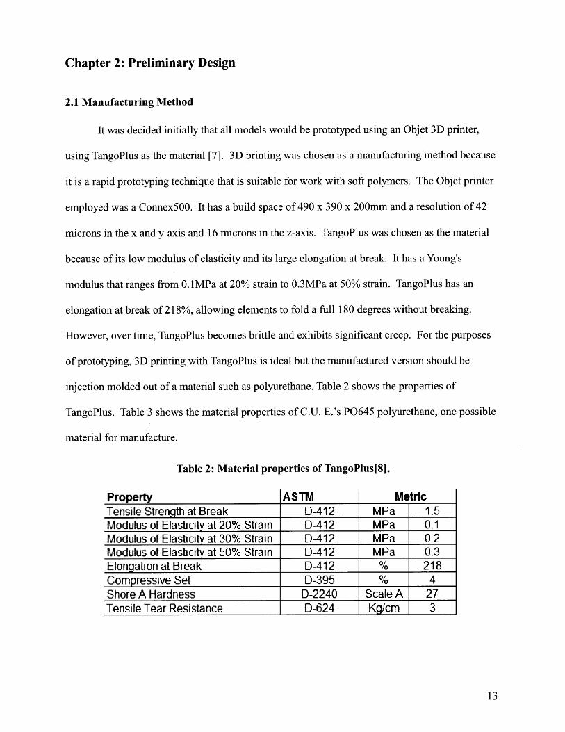
injection molded out of a material such as polyurethane. Table 2 shows the properties of
TangoPlus. Table 3 shows the material properties of C.U. E.'s P0645 polyurethane, one possible
material for manufacture.
Table 2: Material properties of TangoPlus[8].
Property ASTM MetricTensile Strength at Break D-412 MPa 1.5Modulus of Elasticity at 20% Strain D-412 MPa 0.1Modulus of Elasticity at 30% Strain D-412 MPa 0.2Modulus of Elasticity at 50% Strain D-412 MPa 0.3Elongation at Break D-412 % 218Compressive Set D-395 % 4Shore A Hardness D-2240 Scale A 27Tensile Tear Resistance D-624 Kg/cm 3

Table 3: Material properties of P0645 Polyurethane[9].
Property ASTM MetricTensile Strength at Break D-412 MPa 15.9Modulus of Elasticity at 50% Strain D-412 MPa 0.6Modulus of Elasticity at 100% Strain D-412 MPa 0.8Modulus of Elasticity at 200% Strain D-412 MPa 1.2Elongation at Break D-412 % 700Compressive Set D-395 % 15Shore A Hardness D-2240 Scale A 47Tensile Tear Resistance D-624 Kg/cm 17.9
2.2 Concept Generation
As described in the introduction, it was decided that the design requirements of a soft
prismatic joint lend themselves to a design employing flexures. From this point however, the
design strategy must be further defined.
There are three main strategies for achieving the large (30%) axial deformations required
by the design parameters. One strategy employs pure axial deformation as illustrated by a piece
of rubber band. A design based on pure axial deformation depends on the use of a super-elastic
material with a low Young's modulus and/or a small cross-sectional area. While this strategy is
able to achieve large deformations given the proper material and geometry, the parameters
needed to achieve large deformations result in a design with very low bending stiffness. Since a
prismatic joint needs high stiffness in bending, this strategy was not pursued.
The second strategy uses combinations of 4-bar linkages oriented in such a manner that
they cause the structure as a whole to stretch or compress when the links move relative to each
other. This strategy can be illustrated by an accordion. Similarly, a third strategy illustrated by a
spring, uses beam bending of a curved beam to produce compression of the structure as a whole.
Since the second and third strategies both depend on beam bending to achieve structure
compression, they can achieve higher deformations at lower forces than the first strategy while

also maintaining a high enough cross section and material modulus to be stiff enough in bending.
For these reasons, the second and third strategies were pursued.
Four design concepts for the prismatic joint were created from these two strategies as
shown in Figure 4. The linkage, bellows and screw are based on the second strategy and the
spring design is based on the third strategy.
linkages bellows screw spring
Figure 4: Four design concepts for a soft prismatic joint.
The three concepts based on 4-bar linkages can be differentiated by the orientation of the
4-bar linkages. Figure 5 illustrates the locations of the 4-bar linkages in the design and how the
structure as a whole moves as the 4-bar linkages and deformed. In the linkage design, the 4-bar
linkages are arranged in rings along the circumference of the structure. In the bellows design,
the 4-bar linkages are swept about the center axis to form the sections of the bellows. In the
screw design, the 4-bar linkages are arranged along the circumference of the structure. Unlike
the linkage and bellows designs whose linkages compress simply when the structure is
compressed, the screw's linkages skew when compressed. This means that axial displacement of
the screw structure is coupled to rotational displacement.

Figure 5: Location of the 4-bar linkages within three of the design concepts.
An embodiment of each design was 3D printed out of TangoPlus and tested qualitatively.
When tested, the spring demonstrated high axial compliance, but also high bending compliance.
In addition it demonstrated almost no restoring force. This behavior was predictable if one
considers that even springs made out of stiff materials (like steel) exhibit considerable axial and
bending compliance. It was determined that a spring made out of a soft material would not be
able to achieve the desired stiffness in bending so this concept was abandoned.
The linkage design was able to achieve the desired compression and appeared to be stiff
enough in bending. However, because the 4-bar linkages need to widen for the structure to
compress, the structure expands radially in compression. In addition, in the embodiment
investigated here, a significant amount of material must bend in order for the structure to
compress. This requires large forces to achieve the desired displacement. While these problems
could be fixed, they posed a large enough challenge that the concept was discarded.
The bellows design also achieved the desired compression. However, as with the linkage
design, when the structure compressed, the structure expands radially. In addition, because a
large amount of material needs to be deformed in order for the structure to compress, high forces
are needed to achieve the desired compression. Moreover, the narrow regions between the
sections of the bellows are very compliant in bending, allowing the structure as a whole to bend
under low forces. For these reasons, the bellows concept was deemed unsuitable.
The screw design that was built and tested employed vertical rods and was actuated with
a rotary force. The first version also used a stiffer 3D printed material, VeroWhite (modulus of

elasticity: 2495 MPa) for the rods. The straight orientation of the rods as well as their stiff
material caused the structure to act very nearly to an ideal screw. This gave the screw a very
high bending stiffness. In addition, since this structure twists to compress, it does not leave its
3D envelope in compression. Also, since very little material needs to deform in order for the
screw to compress, it takes very low force to compress compared to the other designs. The
structure also has enough restoring force to decompress with no actuation. While all of the
designs possessed the potential to fulfill the design requirements, the screw design seemed to be
the most promising, and so it was pursued. Figure 6 shows the results of the first round of
qualitative testing.
bellows linkage
difficult to compress, bulges when difficult to compress, bulgescompressed when compressed
screw sprng
compresses well, stress compresses well, too floppy, noconcentrations cause breaks spring-back
Figure 6: Results from qualitative testing of the four design concepts for the prismaticjoint.
Table 4 shows a Pugh chart of the results. The Pugh chart employs a simple sponge as
the datum. A sponge is used as the datum because it is a structure that is capable of large
deformations, exhibits a restoring force and can be manufactured using a 3D printer. For

qualitative testing, a piece of a kitchen sponge was used in order to compare sponge behavior to
the printed models.
Table 4: Pugh chart for the four concepts. A sponge is used as a datum.
sponge spring linka e bellows screwaxial compliance 0bending stiffness 0axial expansion 0restoring force 0
18
Chapter 3: Design Parameters of Selected Concept
The next step in the design process was to improve the screw design. One area of focus
was finding a way to reduce the stress concentrations between the stiff rods and the compliant
discs. While the stiff rods provide a large advantage in bending and do not compromise the
movement of the joint in compression, preliminary testing showed that stress concentrations at
the interfaces of materials with largely differing moduli of elasticity are largely intractable. The
dual-material design was thus abandoned in favor of a single material design made entirely out
of TangoPlus.
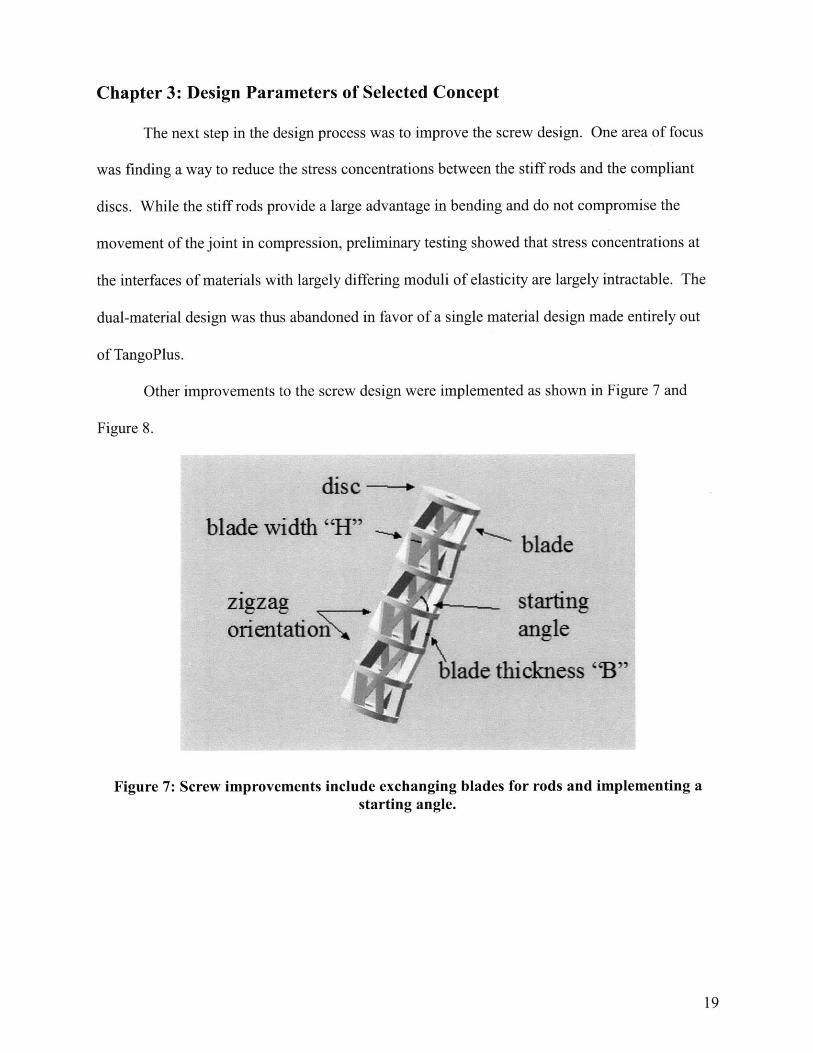
Other improvements to the screw design were implemented as shown in Figure 7 and
Figure 8.
disc -.
blade width "dH"
igzagAorientation
blade
startingangle
thickness "B"
Figure 7: Screw improvements include exchanging blades for rods and implementing astarting angle.

B starting angle
Figure 8: Close up of improved screw design.
Changing the rod material from the stiffer VeroWhite to the more compliant TangoPlus
causes the structure as a whole to become less stiff in bending. In order to gain back this
stiffness, the rods were extended into blades. In theory, this new geometry increases the rods'
contribution to the stiffness of structure in bending. When the structure compresses, each blade
folds over its compliant axis, providing little resistance to the motion. However, when the joint
is loaded radially, the blades at the top and bottom of the joint are loaded radially about their stiff
axis, causing the structure as a whole to exhibit increased stiffness in bending.
A starting angle for the blades was incorporated so that the screw could be actuated
linearly. In the original screw design, the blades were oriented vertically so that the screw had to
be actuated rotationally. While incorporating a starting angle reduces the overall allowable
compression of the joint, the added functionality of linear actuation was deemed worthwhile.
With the implementation of a starting angle, the designer can now decide the direction
that each layer of the screw rotates. Where before with the rotational actuation, all of the layers
of the screw had to rotate in the same direction, with the starting angle the direction of rotation
could be alternating layer by layer allowing the structure as a whole to have no net rotation when
compressed. This also allows every second disc to have no rotation, hence there is a place to
connect the feet that won't rotate.
With these changes, the design concept was finalized. A model of the final concept is
shown in the in Figure 9. This prepared the stage for the next step in the design process of

quantitatively optimizing the concept.
Figure 9: Final concept.

Chapter 4: Modeling
There are some definitions that will be used for rest of this thesis. A single layer of the
joint consisting of a layer of blades and a single disc is considered a single "cell". This is a
useful concept because if behaviors can be established for a single cell, they can be extended to
describe a larger structure by considering combinations of cells in series and in parallel. A
photograph of a single cell is shown in Figure 10.
Figure 10: A single cell with stiff caps on the top and the bottom to help secure the sample.
When discussing designs, Ieq is defined as the area moment of inertia of the joint in
bending. Aeq is defined as the cross-sectional area that a solid cylinder would need to possess to
have the same stiffness in compression as the sample. The ratio of these two values, here called
the "stiffness ratio", is used as a metric for the performances of the design. This metric can be
used to determine how close a structure is to an ideal prismatic joint.
In addition, for this thesis, the labels Ix and Iy are used to discuss the area moments of
inertia of a single blade. Ix is the area moment of inertia of a blade in its stiff direction and Iy is
its area moment of inertia in the compliant direction. These conventions are shown in Figure 11.

H
Figure 11: Area moment of inertia conventions for a blade.
After choosing the screw concept, the design was evaluated and optimized. A model of
the design was presented and evaluated. The model presents a mathematical relationship
between the parameters (blade dimensions, starting angle etc) and the performance of the joint.
A verified model of this type would allow the parameters to be adjusted in order to tune the
performance of the joint as a whole. It is also desired to be able to predict if a design will fulfill
the defined design parameters based on the performance of a single cell or pair of cells. This
chapter presents a metric for this use.
The proposed model is as follows: In compression, a single cell behaves as a group of
beams all bending over their own compliant axes. In bending, the structure acts as a single beam
bending along its stiff direction over a neutral axis a half radius from the center of the ring. The
bending model is illustrated in Figure 12.

H neutral axis
RW2
R
Figure 12: Ring model for structure in bending
This model was arrived at based on qualitative observations of the test cells. The model
for axial compression was decided on based on observation and intuition. The model for
bending is less intuitive and was arrived at as follows: As is always the case in bending, if a
radial load is applied to a cell, one side is put into tension and the other side is put into
compression. In this case, the cells were observed to bend over a neutral axis midway between
the center axis of the cell and the tensioned edge of the cell. It was also observed that the blades
on the compressed side of the cell did not hold their original orientation under load but rather
folded along their compliant axis. This suggests that the only resistance to bending comes from
the blade or blades on the tensioned side of the cell.
This model can be codified into equations as follows: Using the equation for bending of
a cantilevered beam, deflection of a blade when the joint is loaded axially can be expressed as
F,,ta, Lba,3 cos(9)
8blade = 3SEI(
where 3blade is the deflection of the blade, F,,,,a is the axial force applied to the joint as a whole,
blade is the length of a single blade, S is the number of blades per cell, 0 is the angle of the
blade from the horizontal and E is the Young's Modulus of the material. I, is the moment of
inertia of a blade in its compliant direction and is defined as

HB 3
~' 12
S appears in Equation (1) because F,,,,, is spread over S blades in parallel. The cos(O) in
Equation (1) accounts for the fact that the load is not radial to the blade.
Using the equation for axial displacement, deflection of the joint as a whole in
compression can be expressed as
total =Fota Ltota
EAeq
where 5,,,al is the deflection of the joint as a whole, LOta is the length of the whole joint, and
Aeqis the equivalent cross-sectional area of the joint as defined earlier. 3 blade and total can be
related according to
3 tot, = SbIade cos(9).
Putting these Equations (1), (3) and (4) together an equation for Aeq is established, given by
3SI, Lo 1eq cos 2 (O)Lblade
Using the model for bending where the entire load in bending is supported by a single blade,
Ieq can be expressed as
Ie = Ie + HB2 2
where R is the radius of the structure and I, is defined as
BH 3
12
The second term of Equation (6) is derived using the parallel axis theorem, assuming that the
neutral axis is half a radius from the outer edge of the joint.
Combining Equation (5) and (6), the stiffness ratio of the structure as a whole can be
(2)
(3)
(4)
(5)
(6)
(7)

modeled as
IX+BR -H )2 Lbe3CO2
Iq +HBj- LHjJL, cos2(8)(8Ie (2 2(8
Aeq 3SIyLtota
The model was evaluated assuming a constant blade angle of 45 degrees. This
assumption is based on the idea that if used in the robot, the joint would be preloaded such that
all displacements were centered about a blade angle of 45 degrees. The assumption of a constant
angle introduces a maximum multiplicative inaccuracy of four into the calculated stiffness ratio
as shown in Figure 13. However, since these are only first order models used to gain insight into
the behavior of the design, this level of inaccuracy is acceptable.
Stiffness Ratio of 4mm x 1mm Sample
0.0002
0.00018
0.00016
0.00014E- 0.00012 + Stiffness
0 1 Ratio at 450.0001 -degrees
0.00008
0.000040
0
0 5 10 15 20 25 30 35 40 45 50 55 60 65 70Blade Angle (degrees)
Figure 13: Stiffness ratio as a function of blade angle
With the model established, the stiffness ratios predicted by the model can be compared
to the measured stiffness ratios of the samples. These results will be presented in the results
chapter.
It is also desired to be able to predict if a design will fulfill the defined design parameters
based on the performance of a single cell or pair of cells. This can be achieved by substituting

the measured behavior of a sample into the buckling equation. Assuming concentric loading, the
buckling equation states that in order not to buckle
Ft,, < R"2ital eq (9)total
must be true.
Substituting
Loa, - "total (10)
Ctotal
into Equation (9) where to,,, is the strain of the joint in compression expressed as a decimal and
,total is the desired compression defined by the design requirements, the equation as a whole can
be rearranged to be written as
total )2
FI,1, 22eq total (total
In this form, the left hand side of the equations is determined by measurement and the
right hand side of the equation is determined by the design requirements. Results from
evaluating Equation (11) are presented in the results chapter.
Chapter 5: Experimental Setup and Results
5.1 Test Sample Design
While the screw design has many parameters that can be varied, the experimenter focused
on the effects of changes in blade dimension thickness, "B", on joint performance. In order to
test the effects of blade width on performance, there are many parameters that must be held
constant. These values were largely determined through intuition and preliminary experiments.
The number of blades per cell was decided based on the observation that only a small range of
number of blades per cell is practical to manufacture. This range spans from three blades per
cell, below which there is no hope for bending stiffness, to six blades per cell, above which there
is not enough room in the cell for the blades to compress fully. It was decided to use five blades
per cell, as this value produced behavior in an appropriate range of maximum compression and
axial stiffness.
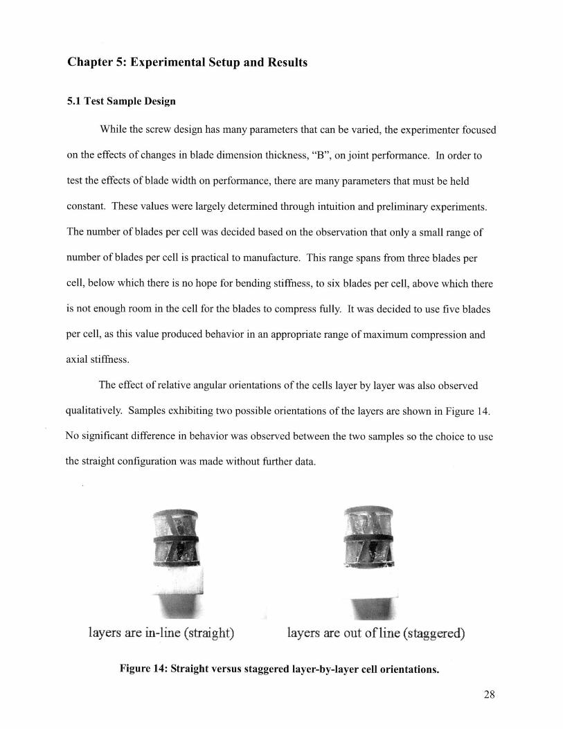
The effect of relative angular orientations of the cells layer by layer was also observed
qualitatively. Samples exhibiting two possible orientations of the layers are shown in Figure 14.
No significant difference in behavior was observed between the two samples so the choice to use
the straight configuration was made without further data.
layers are in-line (straight) layers are out of line (staggered)
Figure 14: Straight versus staggered layer-by-layer cell orientations.

Several other parameters were defined through intuition. The height of the cells was set
at 5mm. This parameter was decided in conjunction with the decision about the number of
blades per cell. Taller cells allow higher overall compression of the joint. However, if the cells
are too tall, the blades will be long enough that they will interfere with each other when the cell
is compressed. The height at which this becomes a problem is thus related to both the cell height
and the number of blades per cell. The combination of 5mm cell height and 5 blades per cell
provided enough room for the cell to compress fully so those values were used.
Disc-thickness was set at 1mm. A trade-off exists for this parameter. Because the discs
act as a dead space for compression, the thicker the discs, the lower the allowable compression of
the cell. However, if the discs are too thin, it was observed that their high compliances
compromise the bending stiffness of the joint overall. This is because the compliant disc folds
and twists into a position where the blades are no longer oriented in their stiff direction. Similar
reasoning was used to set the diameter of the hole in the center of the discs to 2mm. This hole is
needed for the actuator. However, if the hole is too large, the disc loses its stiffness resulting in
the increased bending compliance described above.
The starting angle of the blades was set to 70 degrees. This value was set using intuition.
Again there is a trade-off. A high starting angle allows room for a larger maximum axial
compression of the cell. However, a high starting angle also means a higher axial stiffness of the
cell because of the high angle between the blade and the force that must bend the blade.
Limits on blade width and thickness were also observed. It was found that with 5 blades
per cell, any blade geometry with a width of more than 2mm produced interference between
blades when the structure was compressed. This caused an instability of the structure. It was
therefore decided to limit blade width to 2mm. It was also found that a blade thickness of 0.5mm
was the minimum thickness that could be 3D printed with accuracy. This observation set the
lower limit for blade thickness.

Seven test models were printed for the experiments. It was decided that tests would be
conducted on samples made up of pairs of cells. A test sample is shown in Figure 15. Pairs of
cells were used instead of single cells to ensure that the length to radius ratio of the samples was
high enough for the tests measure bending and not shear. In addition, all test models were 3D
printed at two times full-size in all dimensions in order to facilitate accurate measurement of
deflections. Since the parameters cited in the previous paragraph apply to the full-scale model,
the test samples have cell height of 10mm, disc thickness of 2mm and blade width of 4mm.
Stiff, square plates were printed onto the bottom and the top of the test models to facilitate proper
constraint in testing.
Figure 15: Test sample made up of two cells plus an additional disc at the bottom and hardplates on either end.
5.2 Instrumentation and setup
Instrumentation and setup of the compression and bending tests are shown in Figure 16
and Figure 17. Axial stiffness was tested by measuring displacement while applying a
compressive axial load of known value to a pair of cells. Bending stiffness was tested by
measuring radial deflection of the free end of a cantilevered pair of cells while applying a known
radial load at the free end.

Figure 16: Photograph and schematic of the compression test setup.
Figure 17: Photograph and schematic of the bending test setup.
Additional preliminary bending tests were conducted by loading the cell-pairs non-
concentrically and measuring the angle made by the top of the upper disc as shown in Figure 18.
While this non-concentric loading examines a realistic scenario, the combined bending and
compression loads bending loads inherent to this test insert too much unnecessary complexity
F, delta
l-I]I
F, delta
I /

into the results. This line of testing was thus abandoned in favor of the two more pure loading
tests described above.
Figure 18: Photograph and schematic of the non-concentric loading test.
5.3 Results and Model validation
The model predicts that blade geometry plays an important role in the performance of the
joint. In order to test this hypothesis, data was collected for seven cell-pairs each with different
blade thicknesses. The set of blade thickness tested are shown in Figure 19.
delta
C__ - U_
NN44 N% %t

H
4 0.5 0.0417 2.66674 0.75 0.1406 4.00004 1 0.3333 5.33334 1.25 0.6510 6.66674 1.5 1.1250 8.00004 1.75 1.7865 9.33334 2 2.6667 10.6667
Figure 19: Blade dimensions and area moments of inertias of all samples.
Figure 20 shows the results of the compression tests. Compression tests were conducted
in order to establish the relationship between axial compressive force and axial displacement.
Each line represents a single sample with the legend indicating which sample goes with which
dataset. Measurement errors in the x-axis were ± 0.5mm based on the limits of measurement
capability using a ruler. The force values on the y-axis were measured using a scale and are
accurate to within 0.02N.
Iy (mm4) I L (mm4)H (mm) IB (mmn)
-------------- --

Force v. Displacement over Different Blade Thicknesses
1.4
1.2
1
0 0.6
0.4
0.2
0
Blade Thickness
* 2mm
* 1.75mmA 1.5mm* 1.25mm* 1mmA 0.75mm
o 0.5mm
Figure 20: Force v. displacement in compression. Each dataset represents a bladethickness.
From the results of the compression tests, it is possible to calculate the axial stiffness of
the structure and hence the measured EAeq. Figure 20 only shows the linear range of sample
compression: the range in which the sample compresses freely in a screw motion. Higher forces
produced additional displacement caused by material deformation of the discs and the fully
flattened blades. Hysteresis of up to 0.3N was observed in the stiffer samples. This could be the
result of the high (70 degree) starting angle of the blades, which causes an initial inefficient
transmission of force to displacement. It is also noted that the 4mm x 0.5mm sample has a
negative y-intercept. This is because the sample is so compliant that it compressed under its own
weight without any applied force.
Figure 21 shows the results of the bending tests. From the results of these tests, it is
possible to calculate the bending stiffnesses of the samples and hence the measured Eleq of each
sample. As with the compression chart, each line represents a single sample, and the legend
indicates the blade thickness of that sample. Measurement errors for displacement were again
y=0.1066x+0.3075 a E
y = 0.0966x + 0.242
y = 0.0569x + 0.1691
y =0.0418x + 0.0911
y= 0.0231x + 0.0548
y = 0.0122x + 0.0159y = 0.0047x -0.011
0 2 4 6 8 10 12
Displacement (mm)

determined to be ± 0.5mm. The force values were again measured using a scale and are accurate
to within 0.02N. Less than 0.05N hysteresis was observed in these tests and what was observed
was attributed to measurement error.
Force v. Displacement over Different Blade Thicknesses
0.45y = 0.0283x + 0.0341
0.4 y = 0.0240x + 0.0106
0.35 -- Blade Thickns
0.3y = 0.0177x + 0.0189 0 2mm
0.25 * 1.75mm
. y = 0.0168x + 0.0093 A 1.5mm0 0.2
LL U 1.25mm
0.15 Ey 010084x +0.0102m
0.1 -A 0.75mm
0.05 y = 0.0072x - 0.0046 0 0.5mm
0 y=0. ?x2-x0.0085
0 2 4 6 8 10 12 14 16
Displacement (mm)
Figure 21: Force v. displacement in bending. Each dataset represents a blade thickness.
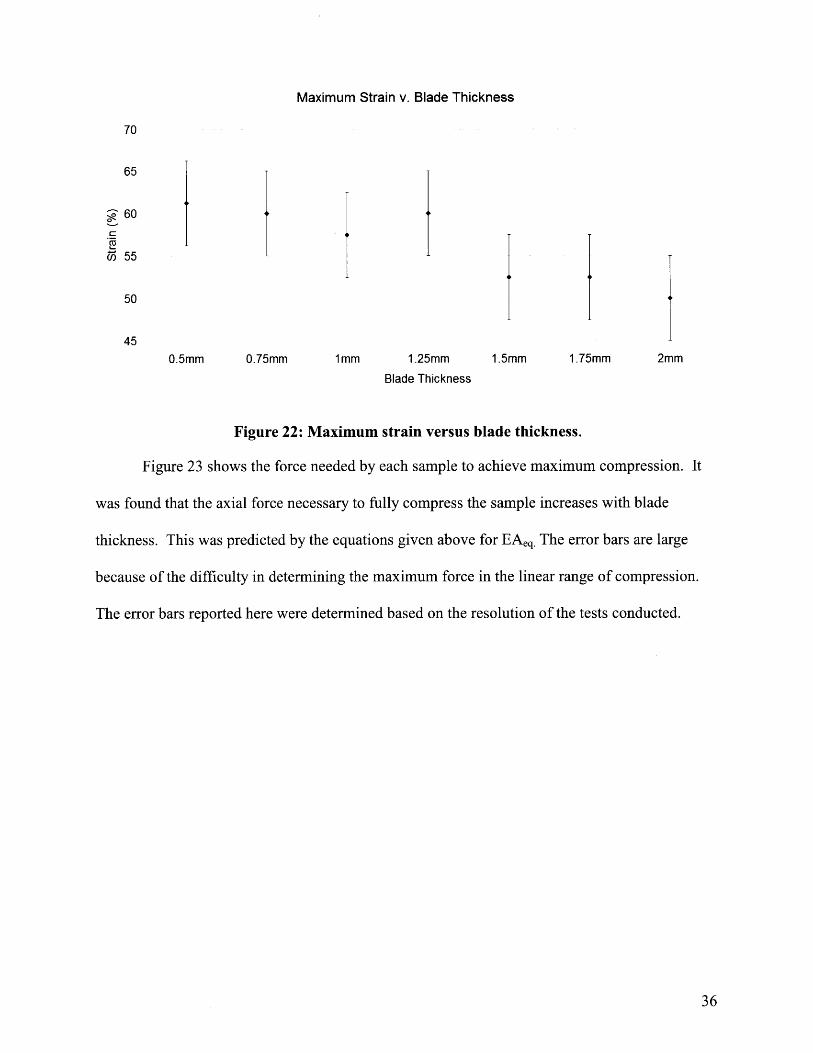
Figure 22 shows a plot of maximum strain versus blade dimensions. It was observed that
maximum strain of the samples increased with decreased blade thickness. This was expected
since compressed cell height is limited by the height of the discs plus the flattened height of the
blades. Thin blades thus allow the cell to compress further than thick blades. The error bars for
these results are larger than for the previous graphs because of the difficulty in determining the
maximum displacement that is still within the linear range of compression. The error bars
reported here were determined based on the resolution of the tests conducted.
Maximum Strain v. Blade Thickness
70
65
60
u5 55
50
450.5mm 0.75mm 1mm 1.25mm 1.5mm 1.75mm 2mm
Blade Thickness
Figure 22: Maximum strain versus blade thickness.
Figure 23 shows the force needed by each sample to achieve maximum compression. It
was found that the axial force necessary to fully compress the sample increases with blade
thickness. This was predicted by the equations given above for EAeq. The error bars are large
because of the difficulty in determining the maximum force in the linear range of compression.
The error bars reported here were determined based on the resolution of the tests conducted.

Force to Compress v. Blade Thickness
1.6
1.41.2
1.0z
0.80.6
0.40.2
0.00.5mm 0.75mm 1mm 1.25mm 1.5mm 1.75mm 2mm
Blade Thickness
Figure 23: The force needed to fully compress the sample versus blade thickness.
Figure 24 compares the measured and calculated values of the stiffness ratio for each
sample. The measured dataset was calculated using the results from the compression and
bending tests reported above. The calculated dataset was computed according to the equations
described in the previous chapter. Error bars are based on the errors accumulated between the
compression and the bending tests as well as the uncertainty inherent in finding a linear fit for
the axial and bending data.

E
0
(I
Stiffness Ratio v. Blade Thickness4.E-04 -
3.E-04
+ measuredcalculated
2.E-04
S1.E-04
n E:AAf'
0.5mm 0.75mm 1mm 1.25mm 1.5mm 1.75mm 2mm
Blade Thickness
Figure 24: Calculated and measured stiffness ratio versus blade thickness.
Figure 24 shows that the calculated stiffness ratio is within a factor of three of the
measured results. As the blades become narrower, the calculated values diverge from the
measured data, suggesting that future work must be done to further develop the model. In
addition, the calculated ratios for the larger blades are lower than what was measured again
suggesting future work on the model.
Figure 25 shows the results from testing the buckling metric established in Equation (11).
The data from the previous tests were gathered to determine if the samples would pass the
buckling test if built to full height as defined by the design requirements. The y-values of the
data points are calculated from the measured values reported above. Y-values for the samples are
given by the left hand side of Equation (11)
Ftoa
EIeq£total2
The grey region at the bottom of the chart is the region where a data point must be in order for
F-1

the sample not to buckle when built to full height. The upper bound of this region is defined by
the right hand side of Equation (11)
( total
where 8 ,,,a is set by the design requirements and equals 24mm. This value is twice that reported
in the design parameters because the samples are two times larger than full-size. This is valid
because buckling scales with size such that a geometry that does not buckle at double size will
also be fine at normal size.
Buckling Criteria v. Blade Thickness
1.2E+05
1.OE+05E
.. 8.OE+04
6.OE+04 _
4.OE+04 -
2.OE+04
0.OE+00 -
0.5mm 0.75mm 1mm 1.25mm 1.5mm 1.75mm 2mm
Blade Thickness
Figure 25: Buckling criteria versus blade thickness. If a sample falls within the greyregion, it will not buckle.
As can be seen, none of the data points are within the non-buckling range. However, if we
take into account the uncertainty of the data as shown with the error bars, it is possible that the
first four samples would not buckle if built to full height. Based on these results, the 1mm
sample was chosen as the best-behaved sample. This blade thickness was chosen because it was
within the range of samples that could potentially resist buckling and, unlike the thinner samples
which were fragile and difficult to constrain fully, it was well-behaved and easy to work with.

5.4 Full scale testing
A full-scale, full-length model was built using a 1mm thick blade. Note however, that
when reduced to 1x scale from the 2x scale model, blade thickness was reduced 0.5mm. It was
found through testing that the full-scale joint did not buckle and was able to achieve the specified
design requirements with the exception of the restoring force. Table 5 shows the results of the
full-scale experiments
Table 5: Results of full-scale experiments.
desired actuallength 4cm 2.3cmdiameter 1cm 1 cmcompression 1.2cm 1.2cmdeflection under own weight 1mm 0.5mmmaterial modulus 1 GPa O2MPaweight 2g 1gforce to actuate 5N 0.2Nrestoring force 1.5N 0.2Ndoes not buckle required achievedno assembly required achievedlow friction mechanism required achieved
Chapter 6: Conclusions and Future Work
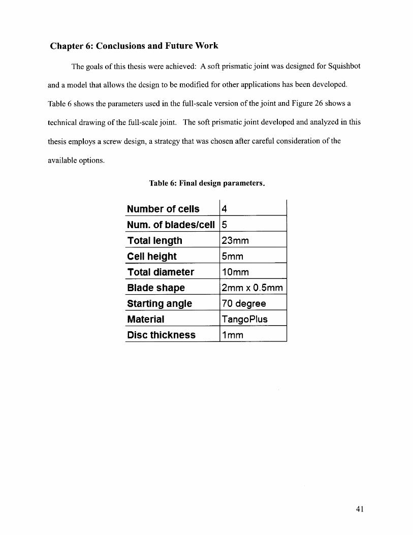
The goals of this thesis were achieved: A soft prismatic joint was designed for Squishbot
and a model that allows the design to be modified for other applications has been developed.
Table 6 shows the parameters used in the full-scale version of the joint and Figure 26 shows a
technical drawing of the full-scale joint. The soft prismatic joint developed and analyzed in this
thesis employs a screw design, a strategy that was chosen after careful consideration of the
available options.
Table 6: Final design parameters.
Number of cells 4
Num. of blades/cell 5Total length 23mmCell height 5mmTotal diameter 10mmBlade shape 2mm x 0.5mm
Starting angle 70 degree
Material TangoPlus
Disc thickness 1mm

~1~~
I J _
Figure 26: Final model of prismatic joint with all dimensions expressed in meters.
In this thesis, sample cells were tested against the model over the blade thickness
parameter space in order to verify the model and determine the optimal parameters for
Squishbot. The final full-scale model was also tested against the original design requirements.
Figure 27 and Figure 28 show the results from testing of the full-scale joint.
Figure 27: Results from testing the full-scale joint in compression.

Figure 28: Results from testing the full-scale joint for softness and as a cantilever.
There are several steps that need to be taken to carry this project forward. The first goal
is to increase the restoring force of the joint such that it is the in the correct range. This can be
achieved by increasing the Young's modulus of the sample material. According to the model,
increasing the modulus of the material does not affect the stiffness ratio of the joint. Increasing
the material stiffness of the joint will increase the softness metric of the joint and the force
needed to actuate it. Both of these values are well below their maximum thresholds so this
solution is predicted to be a success.
Future work is also needed to integrate this joint design into a working robot.
Consideration must be taken regarding how and where to attach feet, how to actuate the joint and
how to connect the joint to the rest of the robot. In addition, this joint needs to be evaluated for
durability over repeated use.
More work needs to be done to improve the accuracy of the model so that it describes the
observed behavior of the joints more closely. A few ways to improve the model have been
considered but not yet implemented. Firstly, the position of the neutral axis is currently
established by qualitative observation. However, it appears that the neutral axis changes position
proportionally to the ratio of Ix/Iy with it moving outwards from the center of the joint as Ix/Iy
increases. If this observation were formalized in the model, it is likely that the calculated

stiffness ratios would better follow the observed stiffness ratios.
The model also assumes that only one blade carries the load in bending. This assumption
appears to be true for five-blade cells but will not hold if the number of blades per cell is varied.
The relationship between the number of blades holding the load and the number of blades per
cell should also be investigated.
In addition, the effect of other parameters on the performance of the joint should be
studied. Blade thickness has been investigated to the limits allowed by geometry and
manufacturing capability. Other parameters to investigate include cell height, disc thickness,
starting angle and building material. As these parameters are investigated, new properties and
behaviors of the joint will emerge and the equations describing the joint's behavior can be
modified.
In addition, the screw design invites the creation of a locking mechanism that is triggered
by a rotational actuator and when activated, prohibits compression. Preliminary work was done
on the development of the locking mechanism shown in Figure 29 and Figure 30. This
mechanism employs legs made out of a stiffer 3D printed material, VeroWhite. With a slight
twist, the legs can be brought into a position where they are pressed against each other,
preventing the structure from compressing.
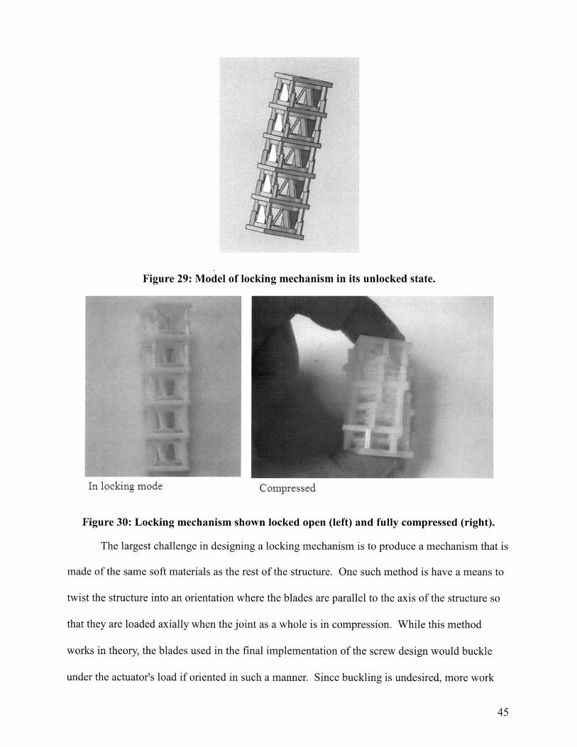
Figure 29: Model of locking mechanism in its unlocked state.
In locking mode Compressed
Figure 30: Locking mechanism shown locked open (left) and fully compressed (right).
The largest challenge in designing a locking mechanism is to produce a mechanism that is
made of the same soft materials as the rest of the structure. One such method is have a means to
twist the structure into an orientation where the blades are parallel to the axis of the structure so
that they are loaded axially when the joint as a whole is in compression. While this method
works in theory, the blades used in the final implementation of the screw design would buckle
under the actuator's load if oriented in such a manner. Since buckling is undesired, more work

needs to be conducted in this area.
With the successful fulfillment of the project's design goals, the work presented in this
thesis is a valuable addition to the Squishbot project. In addition, the work presented here adds
to the platform of soft prismatic design and can be used for future soft robotics development.
This project invites a host of future work, indicating that is a rich area for future research. The
design presented in this thesis is almost ready for integration into Squishbot, an existing soft
robot. Future work could complete this integration and enable this design to be applied to other
soft robots.

References
[1] http://www.darpa.mil/dso/thrusts/materials/multfunmat/chembots/index.htm
[2] Cheng, N., Ishigami, G., Hawthorne, S., Chen, H., Hansen, M., Telleria, M., Playter, R., andIagnemma, K., "Design and Analysis of a Soft Mobile Robot Composed of Multiple ThermallyActivated Joints Driven by a Single Actuator," IEEE International Conference of Robotics andAutomation, 2010.
[3] Telleria, M., Hansen, M., Campbell, D., Servi, A., and Culpepper, M., "Modeling andImplementation of Solder-activated Joints for Single-actuator, Centimeter-scale RoboticMechanisms," IEEE International Conference on Robotics and Automation, 2010
[4] Cheng, N., Ishigami, G., Hawthorne, S., Chen, H., Hansen, M., Telleria, M., Playter, R., andIagnemma, K., "Design and Analysis of a Soft Mobile Robot Composed of Multiple ThermallyActivated Joints Driven by a Single Actuator," IEEE International Conference of Robotics andAutomation, 2010.
[5] Cheng, N., Ishigami, G., Hawthorne, S., Chen, H., Hansen, M., Telleria, M., Playter, R., andlagnemma, K., "Design and Analysis of a Soft Mobile Robot Composed of Multiple ThermallyActivated Joints Driven by a Single Actuator," IEEE International Conference of Robotics andAutomation, 2010.
[6] Smith, Stuart A, Flexures: Elements ofElastic Mechanisms, USA: CRC Pres, 2000.
[7] http://objet.com/3D-Printer/Connex500/
[8] http://objet.com/Materials/TangoMaterials/
[9] http://www.cue-inc.com/technical-data-charts.html