Embed Size (px)
Citation preview

International Journal of Latest Engineering Research and Applications (IJLERA) ISSN: 2455-7137
Volume – 02, Issue – 07, July – 2017, PP – 77-85
www.ijlera.com 2017 IJLERA – All Right Reserved 77 | Page
Design and CFD Analysis of a Fixed Wing for an Unmanned
Aerial Vehicle
Karthik M A1, Srinivasan K2, Srujan S 3, Subhash Holla H S 4, Suraj Jain M 5, 1(Assistant Professor, Department of Mechanical Engg, Dayananda Sagar College of Engineering, India)
2,3,4,5(Student, Department of Mechanical Engineering, Dayananda Sagar College of Engineering, Bengaluru, India)
Abstract: The present boom in the drone industry and its apparent low impact in India was the raison d'être for
the decision to design and analyze a fixed wing for an unmanned aerial vehicle which would serve as a
multipurpose utility tool. The paper describes the need for such a tool and its use. Adopting a design procedure
that is used by institutions like NAL, HAL, etc. a three-dimensional model of a flying wing was done. This
iterative process was followed by the flow analysis of half the plane in Fluent which was initially meshed in
ICEM CAD. The analysis yielded the lift and drag forces. This aided in the structural analysis of the wing
section which was done considering the wing to be made of EPP (Expanded poly- propylene). The wing
structure analysis helped us realize that the design well below the strength limit even with a big factor of safety.
This followed the modal analysis of the system, for which the approximate fundamental frequency was initially
calculated. The modal analysis verified the calculation with a very low error percentage. The entire process
resulted in a flying wing which can be rolled out commercially with minimal designchanges.
Keywords: Drones, Aerofoils, Fixed Wings, CFD, XFLR5, Structural Analysis
I. INTRODUCTION In modern days, man power is being replaced by machines to make the process more efficient. One
such replacement are drones. The term “drones” covers a very broad category of unmanned aerial vehicles
(UAV) that can be used for anything from military or commercial purposes, topersonalentertainment. Drones are
being used to carry out aerial mapping, rescue operations, land surveying, military operations and various other
applications. Despite of its extensive usage in many countries, India lags in its effective usage. Europe is one
such country which has used this technology effectively, especially in the field of agriculture. Drones are being
used to monitor the crops and identify the reasons for crop failures to increase the crop yield. With the help of
drones, overall yield was increased by 15 percent. The drones being used in Europe were found to be costly
whereas on the other hand, the drones used in India were found to be inefficient. So, we decided to design a
model which would be both effective and costefficient.
The drones which are being used today are quad copters and fixed wing type. We decided to go with
the fixed winged type because they are found to be more suitable for mapping purposes. After comparing
various models which are commercially available, we found eBee and sky walker to be the basis for our model.
The calculations to make the basic design of the model were made referring many books. The 2D model of the
drone was made using the calculated parameters. Various standard aero foils were analyzed in XFLR5 to select
the best one. Using the selected aero foil, the wings of the model were designed in Solid works software. A
standard fuselage was selected which was assembled with the designed wings in CATIA software to obtain the
final 3-dimensional model. This finished model was subjected to CFD analysis wherein one half of the model
was tested in a wind tunnel by applying boundary conditions. The model gave positive results in the CFD
analysis. Further, the model was subjected to modal and structural analysis to determine the fundamental
frequency of the model. The designed model is more aerodynamically stable than the commercially available
models.
II. EXPERIMENTAL DETAILS The basic requirements for our flight are:
Modulardesign
High altitudeflight(50-100m)
High speedflight(15-30ms-1
)
Sweptback
Sturdy material like EPPfoam
No take-off and landing area required

International Journal of Latest Engineering Research and Applications (IJLERA) ISSN: 2455-7137
Volume – 02, Issue – 07, July – 2017, PP – 77-85
www.ijlera.com 2017 IJLERA – All Right Reserved 78 | Page
Maximum velocity 50ms-1
Wing loading maximum 6kg/m2
Span maximum 1.5m
For the design, related calculations eBee and sky walker x8 are referred. The values considered are mentioned in
the below mentioned table.
eBee Sky walker X8
1. Wing span 0.96m 2.12m
2.Cruise speed 11-25 ms-1
15.27-30.556ms-1
3.Wing area 0.5m2
0.8m2
4.Pay load Approx. 1.5kg 1-2 kg
5.Weight 0.71kg 0.88kg
Table 1. Comparison of eBee and Skywalker X8
2.1 Design
Preliminary Assumptions Made
1. Wing Area – 0.6 m2
2. Wing span – 1.5 m2
3. Sweep angle – 30o
4. Taper Ratio – 0.75
5. Aspect Ration – 3.75
Figure 1. Taper ratio graph
2. Basic Calculations OutputTable 3. Location of spars, propellers, etc.
2.2Aero foil Selection
To decide the suitable aerofoil, few aerofoils were considered and their co-ordinates were taken from UIUC
library and were compared using XFLR5 software.
The aerofoils considered were:-

International Journal of Latest Engineering Research and Applications (IJLERA) ISSN: 2455-7137
Volume – 02, Issue – 07, July – 2017, PP – 77-85
www.ijlera.com 2017 IJLERA – All Right Reserved 79 | Page
MH-44
MH-45
S-5010
MH-60
MH-64
Eh 2.0/10.0
2.3 Test Criterion
Reynolds number = ρ*V*D/µ
Reynolds number = 1, 00,000-10, 00,000 with an increment of 50,000
Angle of attack- (-10o TO +10
o) with an increment of 0.5
o
Mach number-0.152
Graphs for below mentioned Reynolds numbers are plotted
Re=200,000 (INITIAL CONDITION)
Re=500,000-550,000 (OPERATING RANGE)
2.4Comparison
The graphs for the aero foils MH45, MH60 and S5010 with values close to our requirements are drawn
and compared: -
Figure 2. XFLR5 analysis of MH45Figure 2. XFLR5 analysis of MH60
Figure 2. XFLR5 analysis of S5010
The first graph gives the ratio of 𝐶𝑙 /Cd where 𝐶𝑙 is the lift coefficient and Cd is the drag coefficient. Lift
coefficient gives the measure of the upward lift force and the drag coefficient is the measure of the force which
acts opposite to the direction of motion. The ratio of 𝐶𝑙 /Cd should be high, i.e., lift coefficient should be as high
as possible and the drag coefficient should be as low as possible. The second graph is a plot of lift coefficient
versus the angle of attack. Angle of attack is the angle at which the wind strikes the aero foil. Lift coefficient
should be higher for low angle of attack. The third graph shows the variation of lift coefficient over the entire
aero foil. The fourth graph shows the variation of𝐶𝑙 /Cd for different angle of attack. 𝐶𝑙 /Cd should be higher for
low angle of attack.
The above said aero foils were also compared based on 𝐶𝑀 vs 𝐶𝑙 , 𝐶𝑙 /𝐶𝐷 vs 𝐶𝑙 and the necessary graphs
are drawn.

International Journal of Latest Engineering Research and Applications (IJLERA) ISSN: 2455-7137
Volume – 02, Issue – 07, July – 2017, PP – 77-85
www.ijlera.com 2017 IJLERA – All Right Reserved 80 | Page
Graphs for on 𝐶𝑀 vs 𝐶𝑙 of MH45, MH60 & S5010
Figure 2. 𝐶𝑀 vs 𝐶𝑙 for MH45 Figure 2. 𝐶𝑀 vs 𝐶𝑙 for MH60
Figure 2. 𝐶𝑀 vs 𝐶𝑙 for S5010
The graph shown above is a plot of 𝐶𝑚 versus 𝐶𝑙 where 𝐶𝑚 is the pitching moment which provides the
required lift. The value of the pitching moment should be high for the calculated lift coefficient which is 0.3.
Graphs for on 𝐶𝑙 /𝐶𝐷 vs 𝐶𝑙 of MH45, MH60 & S5010
Figure 2. 𝐶𝑙 /𝐶𝐷 vs 𝐶𝑙 of MH45 Figure 2. 𝐶𝑙 /𝐶𝐷 vs 𝐶𝑙 of MH60

International Journal of Latest Engineering Research and Applications (IJLERA) ISSN: 2455-7137
Volume – 02, Issue – 07, July – 2017, PP – 77-85
www.ijlera.com 2017 IJLERA – All Right Reserved 81 | Page
Figure 2. 𝐶𝑙 /𝐶𝐷 vs 𝐶𝑙 of S5010
The graph shown above is a plot of 𝐶𝑙 /𝐶𝑑 versus 𝐶𝑙 . The ratio of 𝐶𝑙 /𝐶𝑑 should be maximum for the
calculated lift coefficient which is 0.3.
MH 45 MH 60 S5010
𝐶𝑙 at 0° AOA 0.12 0.12 0.14
𝐶𝑙 at 5° AOA 0.68 0.68 0.70
𝐶𝑚 at 𝐶𝑙 =0.21 -0.01 -0.01 0.00735
𝐶𝑙 /𝐶𝑑 at 𝐶𝑙=0.21 27.5 27.5 27.5
Table 4. Comparison of MH45, MH60 and S5010
From the abovegraphs and results,S5010 foil has better lift, lesser drag and closer pitching moment to required
value.
2.4 Design
Selected Aero-foil S5010 is designed to the requirements. 2-Dimensional and Isometric view of the
selected aero-foil is shown below.
Figure 2. Two-Dimensional Outline of the Plane Figure 2. Isometric view of the final design.
3. CFD ANALYSIS Flow analysis is the simulation of air flow over given interest area and the tabulation of interaction
between air flow and surface area. [2]. Classical models based on Reynolds Averaged Navier-Stokes (RANS)
equations (time averaged) are:
Zero equation model:
Mixing length model.
One equation model
Two equation models
k- ε style models (standard, RNG, realizable)
k-ω model, and
ASM.
Seven equation models
Reynolds stress model.

International Journal of Latest Engineering Research and Applications (IJLERA) ISSN: 2455-7137
Volume – 02, Issue – 07, July – 2017, PP – 77-85
www.ijlera.com 2017 IJLERA – All Right Reserved 82 | Page
3.1 K- ε Model
The k–ω family of turbulence models have gained popularity mainly because:
The model equations do not contain terms which are undefined at the wall, i.e. they can be integrated to
the wall without using wall functions.
They are accurate and robust for a wide range of boundary layer flows with pressure gradient.
FLUENT offers two varieties of k–ω models. [3]
Standard k–ω (SKW) model
Most widely adopted in the aerospace and turbo-machinery communities.
Several sub-models/options of k–ω: compressibility effects, transitional flows and shear-flow
corrections.
Shear Stress Transport k–ω (SSTKW) model
The SST k–ω model uses a blending function to gradually transition from the standard k–ω model
near the wall to a high Reynolds number version of the k–ε model in the outer portion of the
boundary layer.
Contains a modified turbulent viscosity formulation to account for the transport effects of the principal
turbulent shear stress.
As the Standard k–ω (SKW) model yielded the most accurate results and consumed the least time we opted to
go for this model.
The design in the. IGES file format was imported from the design software (CATIA), but only half of the entire
design was used for analysis. This was because, the processing time and power required for the entire plane to
be analyzed was very high.
3.2 Methodology of CFD Analysis
3.2.1 Pre – Processing
Figure 9. Part wing geometry taken from CATIA design.
Wing is placed inside the wind tunnel by creating an enclosure with approximate dimensions. The case study
starts with geometry clean up followed by naming the inlet, outlet and boundaries.
3.2.2Boolean Subtraction
Figure 10. shows the Boolean subtraction

International Journal of Latest Engineering Research and Applications (IJLERA) ISSN: 2455-7137
Volume – 02, Issue – 07, July – 2017, PP – 77-85
www.ijlera.com 2017 IJLERA – All Right Reserved 83 | Page
It is followed by Boolean subtraction wherein only the fluid geometry is kept by subtracting the part wing
geometry from the work volume.
3.2.3 Meshing
Figure 11. shows the discretized workspace
The discretization of wing body along with wind tunnel set is carried out by specifying appropriate rate
of refinement, which was set to fine to carry out the discretization process.
4. SOLUTIONS The module for solving the problem on hand was selected to be K omega turbulence module over
Spalart alaramas. These two are the only module that could have been used for closed work surfaces out of
which K epsilon module gave more accurate results and hence it was used for the analysis.
Boundary conditions:
Cruise velocity: 50ms-1
(The operating speed will be in the range of 25ms-1
which ascertains better
results)
Kinematic viscosity: 15.5 *10e-6 m2/sec
Density of air: 1.22kg/m3
4.1 Post Processing
4.1.1 Velocity Streamline
Figure 11. Shows the stream line velocity
The flow lines of all the particles are shown and it is seen that majority lie in the range of 47.79ms-1
.
International Journal of Latest Engineering Research and Applications (IJLERA) ISSN: 2455-7137
Volume – 02, Issue – 07, July – 2017, PP – 77-85
www.ijlera.com 2017 IJLERA – All Right Reserved 84 | Page
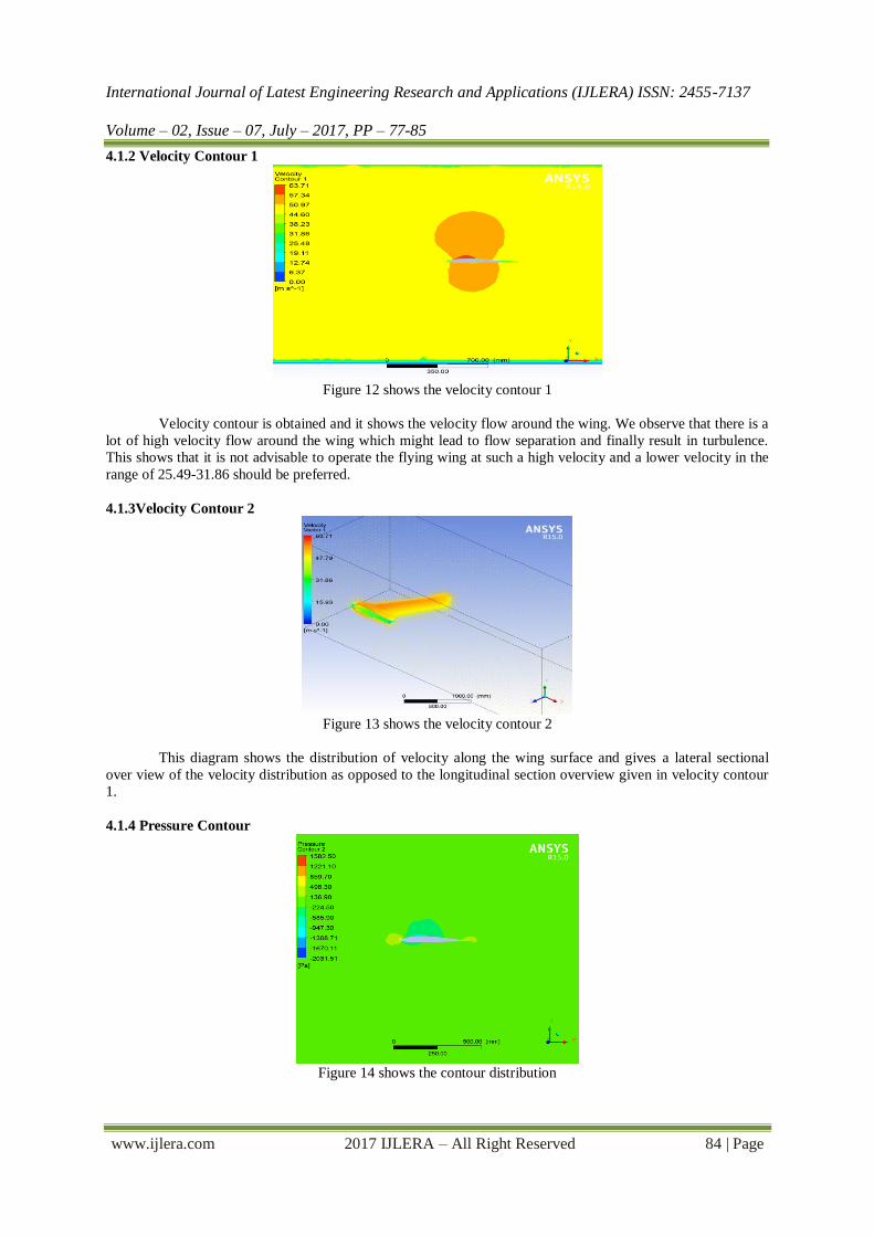
4.1.2 Velocity Contour 1
Figure 12 shows the velocity contour 1
Velocity contour is obtained and it shows the velocity flow around the wing. We observe that there is a
lot of high velocity flow around the wing which might lead to flow separation and finally result in turbulence.
This shows that it is not advisable to operate the flying wing at such a high velocity and a lower velocity in the
range of 25.49-31.86 should be preferred.
4.1.3Velocity Contour 2
Figure 13 shows the velocity contour 2
This diagram shows the distribution of velocity along the wing surface and gives a lateral sectional
over view of the velocity distribution as opposed to the longitudinal section overview given in velocity contour
1.
4.1.4 Pressure Contour
Figure 14 shows the contour distribution

International Journal of Latest Engineering Research and Applications (IJLERA) ISSN: 2455-7137
Volume – 02, Issue – 07, July – 2017, PP – 77-85
www.ijlera.com 2017 IJLERA – All Right Reserved 85 | Page
The diagram shows that the pressure variation and the maximum pressure on the entire part geometry
does not exceed -585.9 Pa and hence a suitable pressure difference required for lift is generated.
4.2 Results
Drag Force, Fdrag (from CFD analysis) = 10.68N
Lift Force, Flift (from CFD analysis) = 40.513N
References: Books:
[1]. “Drones”, LiveScience.com, http://www.livescience.com/topics/drones?type=article
[2]. T.S.D. Karthik, 2011. “Turbulence Models and Their Applications”, 10th Indo German Winter
Academy 2011
[3]. “Modeling Turbulent Flows”, ANSYS Introductory FLUENT Training.
[4]. [4] Von Mises Stress, www.continuummechanics.org,
http://www.continuummechanics.org/vonmisesstress.html
[5]. Gerrit Visser, 2011. “Modal Analysis: What it is and is not”, ESTEQ, 25 November 2011.
https://esteq.co.za/2014/11/25/modal/
Theses:
[6]. Rupak Biswas and Roger C. Strawn, 1997. “Tetrahedral and Hexahedral mesh adaptation for CFD
problems”, NASA Tech reports. https://www.nas.nasa.gov/assets/pdf/techreports/1997/nas-97-007.pdf


![Blended Wing’ CFD Analysis: Aerodynamic Coefficients. · airfoils at low Reynolds numbers, such as the XFLR5 [5, 7]. Nevertheless, the values obtained through this software are](https://img.pdfslide.net/doc/110x75/5e68547c68b2a32bb7246be4/blended-winga-cfd-analysis-aerodynamic-airfoils-at-low-reynolds-numbers-such.jpg)