Embed Size (px)
Citation preview
Western Michigan University
Department of Aeronautical and Mechanical Engineering
December 2007
Design and Control of an Inverted Pendulum
Design Team:
Andrew Hovingh
Matt Roon
Faculty Mentor:
Dr. James Kamman
Industrial Mentor:
Dr. James Kamman
ME480 Final Project Report
ME 0712-05

Design and Control of an Inverted Pendulum
By
Andrew Hovingh
Matt Roon
Reviewed By: ______________________________
______________________________
______________________________
Approved By: _____________________________
Summary: This work was done during the period 9/18/2007 –12/4/2007 for Dr. James Kamman
and the Western Michigan University Motion and Control Lab.
i
Abstract
An inverted pendulum, usually mounted on a cart actuated by an applied force, was designed and built for an existing hydraulically driven sled or cart. This particular sled was constrained to one axis along the horizontal plane of the base apparatus. Position information of the cart was acquired via a LVDT (Linear Variable Differential Transformer) sensor, and a digital sensor (angular incremental encoder) was used to sense the pendulum angle, which was collected by a computer containing a DAQ (Data Acquisition) card and running LabVIEW software. A LabVIEW graphical program was implemented as a controller of the hydraulic system that governed the motion of the sled in order to maintain vertical balance of the inverted pendulum.
The purpose for this type of experiment was to test different algorithms used to control mechanical systems. Examples of specific algorithms that regulate mechanical systems are proportional integral derivative (PID) and any combination of the three types. Control over mechanical systems is a vastly engulfing industry today by means of automation processes. These automation processes may be implement for various reasons, ranging from increased safety to optimization of performance.
Executing this experiment began by mathematically modeling the physical system. A number of software tools were developed to aid in the process of modeling and analyzing simulation data. Simulating the response to the system based on varying parameters, the team determined part specifications and requirements. After parts were designed and attained, the mechanical system was assembled for experimentation and analysis of results. The inverted pendulum successfully maintained a relative range of pendulum angle for the prescribed time of 15 seconds using PI control.

ii
Disclaimer
The following information is intended for educational purposes only. It does not
constitute a legal contract between Western Michigan University and any person or entity. This
project was completed as a student endeavor, not to be considered for industrial use. The
students and staff involved in the project will not be held responsible for misuse or
misinterpretation of any materials.
iii
Table of Contents
Abstract .......................................................................................................................................................... i Table of Contents ......................................................................................................................................... iii Table of Figures ............................................................................................................................................ vi List of Tables ................................................................................................................................................ ix Nomenclature ............................................................................................................................................... x 1. Introduction ..................................................................................................................................... 1
1.1. Background ................................................................................................................... 1 1.2. Problem Description ..................................................................................................... 2 1.3. Need .............................................................................................................................. 3 1.4. Goal ............................................................................................................................... 3 1.5. Impact ........................................................................................................................... 3
1.5.1. Environmental Impact .............................................................................. 3 1.5.2. Global Impact ............................................................................................ 4 1.5.3. Impact on Society ..................................................................................... 4
2. Requirements and Specifications .................................................................................................... 4 2.1. Functional Requirements .............................................................................................. 4 2.2. Physical Specifications .................................................................................................. 5 2.3. Safety Specifications ..................................................................................................... 6 2.4. Software Specifications ................................................................................................. 6 2.5. House of Quality and QFD ............................................................................................. 7
3. Concept Exploration......................................................................................................................... 9 3.1. Benchmarking ............................................................................................................... 9 3.2. Physical Decomposition .............................................................................................. 14 3.3. Function Decomposition ............................................................................................. 14 3.4. Form Decomposition ................................................................................................... 17
4. Cost Analysis .................................................................................................................................. 18 5. Project Schedule ............................................................................................................................ 20 6. Design............................................................................................................................................. 20
6.1. Physical System Design ............................................................................................... 20 6.1.1. Background ............................................................................................. 20 6.1.2. Concept ................................................................................................... 21
6.1.2.1. Custom Configurable Parts ........................................................ 22 6.1.3. Proposed Configuration .......................................................................... 22
6.1.3.1. Pendulum Design ....................................................................... 22 6.1.3.1.1. Components and Materials ................................................. 23 6.1.3.1.2. Sizing .................................................................................... 25
6.1.3.2. Pivot Joint Design ....................................................................... 29 6.1.3.2.1. Components and Materials ................................................. 29 6.1.3.2.2. Sizing .................................................................................... 32
6.1.3.3. Fixture Design ............................................................................ 37 6.1.3.3.1. Components and Materials ................................................. 37 6.1.3.3.2. Sizing .................................................................................... 42
6.1.3.4. Electrical Hardware .................................................................... 53 6.1.3.4.1. Sensor Design and Specifications ........................................ 53
6.1.3.4.1.1. Analog vs. Digital ................................................. 57
iv
6.1.3.4.2. DAQ Card Integration .......................................................... 61 6.1.4. Final Physical System Configuration ....................................................... 63
6.2. Software and Control Design ...................................................................................... 67 6.2.1. MATLAB and Software Tools .................................................................. 67
6.2.1.1. Introduction ............................................................................... 67 6.2.1.2. Overall Process .......................................................................... 67 6.2.1.3. Calibration Files ......................................................................... 69
6.2.1.3.1. Calibration File Description ................................................. 69 6.2.1.3.2. Calibration File Structure ..................................................... 69 6.2.1.3.3. Variable Assignments in Calibration Files ............................ 71
6.2.1.4. Calibration Tools ........................................................................ 73 6.2.1.4.1. Calibration Tools Introduction ............................................. 73 6.2.1.4.2. makeFunction.m .................................................................. 73 6.2.1.4.3. makeCalibration.m .............................................................. 74 6.2.1.4.4. makeCalInLikeness.m .......................................................... 77 6.2.1.4.5. getPIDGains.m ..................................................................... 77 6.2.1.4.6. checkParameters.m ............................................................. 80 6.2.1.4.7. chooseCalibrationSet.m ....................................................... 81 6.2.1.4.8. getCalibrationSet.m ............................................................. 82
6.2.1.5. Simulink Models and Tools ........................................................ 82 6.2.1.5.1. Models Introduction ............................................................ 83 6.2.1.5.2. System Model ...................................................................... 83 6.2.1.5.3. Model Tools ......................................................................... 88
6.2.1.6. Model Results and Tools ............................................................ 90 6.2.1.6.1. animationGUI.m .................................................................. 91 6.2.1.6.2. makePendulumAnimation.m ............................................... 93 6.2.1.6.3. getPerformanceResults.m ................................................... 94 6.2.1.6.4. graphResults.m .................................................................... 96
6.2.2. System Identification .............................................................................. 97 6.2.2.1. Hydraulic Valve and Cylinder Dynamics .................................... 98 6.2.2.2. Dry Friction .............................................................................. 103
6.2.3. Data Acquisition and Control Tools ...................................................... 105 6.2.3.1. Introduction to Real Time Control Tools ................................. 105 6.2.3.2. Controller Front Panel ............................................................. 106
6.2.3.2.1. Front Panel Angle Initialization Mode ............................... 107 6.2.3.2.2. Front Panel Main Mode ..................................................... 109
6.2.3.3. Controller Block Diagram ......................................................... 112 6.2.4. Controller Design .................................................................................. 118
6.2.4.1. Open Loop System ................................................................... 118 6.2.4.2. Control Design Using Emulation .............................................. 119 6.2.4.3. PI Controller Design ................................................................. 121 6.2.4.4. Controller Difference Equation ................................................ 124
7. Results .......................................................................................................................................... 125 7.1. Conclusions ............................................................................................................... 129 7.2. Lessons Learned ........................................................................................................ 131 7.3. Recommendations .................................................................................................... 133
8. Bibliography ................................................................................................................................. 135
v
9. Acknowledgements...................................................................................................................... 136 Appendix A: Equations............................................................................................................Appendix A-1 Appendix B: MATLAB Programs ............................................................................................. Appendix B-1 Appendix C: SIMULINK Models ............................................................................................... Appendix C-1 Appendix D: LabVIEW Programs ........................................................................................... Appendix D-1 Appendix E: CAD Drawings .................................................................................................... Appendix E-1 Appendix F: Price Quotes ....................................................................................................... Appendix F-1 Appendix G: Pictures of Physical System ............................................................................... Appendix G-1 Appendix H: Simulation Results ............................................................................................. Appendix H-1 Appendix I: Approach ............................................................................................................. Appendix I-1 Appendix J: Resumes ..............................................................................................................Appendix J-1 Appendix K: ABET Assessments .............................................................................................. Appendix K-1
vi
Table of Figures
Figure 1 - Motion and Control Laboratory .................................................................................................... 2 Figure 2: House of Quality Matrix ................................................................................................................. 8 Figure 3: House of Quality Interaction Matrix .............................................................................................. 9 Figure 4: Rotational and Water Disturbance System .................................................................................. 10 Figure 5: Adjustable Bob Weight System .................................................................................................... 11 Figure 6: Seesaw System ............................................................................................................................. 11 Figure 7: Tilt Sensor and Cart System ......................................................................................................... 12 Figure 8: Rotational System ........................................................................................................................ 13 Figure 9: Energy Flow .................................................................................................................................. 16 Figure 10: Material Flow ............................................................................................................................. 17 Figure 11: Information Flow ....................................................................................................................... 17 Figure 12: Physical System Parts Reference ............................................................................................... 18 Figure 13: Gantt Chart / Project Schedule .................................................................................................. 20 Figure 14: Motion and Control Laboratory ................................................................................................. 21 Figure 15: PIPA15-900 Pendulum Bar ......................................................................................................... 23 Figure 16: PSCCN15-10 Shaft Collar Assembly ............................................................................................ 24 Figure 17: Pendulum Bob and Shaft Collars (Assembly) ............................................................................. 25 Figure 18: Pendulum Rod Schematic .......................................................................................................... 26 Figure 19: Pendulum Rod Catalog Reference ............................................................................................. 27 Figure 20: Shaft Collar Schematic ............................................................................................................... 28 Figure 21: Shaft Collar Catalog Reference .................................................................................................. 29 Figure 22: BGHWA6200ZZ-30-40 Bearing Mount Assembly ....................................................................... 30 Figure 23: PHFRZ15-100.0-F50.0-B20-P10-T50.0-S20-Q10 Rotary Shaft .................................................... 31 Figure 24: Bearing Mount Schematic .......................................................................................................... 33 Figure 25: Sensor Coupling Catalog Reference 2 ........................................................................................ 44 Figure 26: Strut Clamp Schematic ............................................................................................................... 46 Figure 27: Strut Clamp Catalog Reference .................................................................................................. 47 Figure 28: Pendulum Stop Support Schematic ........................................................................................... 48 Figure 29: Pendulum Stop Support Catalog Reference .............................................................................. 49 Figure 30: Base Plate Schematic ................................................................................................................. 50 Figure 31: Angle Encoder Mount Schematic ............................................................................................... 51 Figure 32: Analog Angle Sensor Mount Schematic ..................................................................................... 52 Figure 33: Angle Encoder ............................................................................................................................ 53 Figure 34: Angle Encoder Catalog Reference .............................................................................................. 54 Figure 35: Angle Encoder Specifications ..................................................................................................... 55 Figure 36: Angle Encoder Schematic 1 ........................................................................................................ 55 Figure 37: Angle Encoder Schematic 2 ........................................................................................................ 56 Figure 38: Angle Encoder Wiring Information 1 ......................................................................................... 56 Figure 39: Angle Encoder Wiring Information 2 ......................................................................................... 57 Figure 40: Analog Angle Sensor .................................................................................................................. 57 Figure 41: Analog Angle Sensor Catalog Reference .................................................................................... 58 Figure 42: Analog Angle Sensor Specifications ........................................................................................... 58 Figure 43: Analog Angle Sensor Schematic ................................................................................................. 59 Figure 44: Analog Angle Sensor Wiring Information .................................................................................. 60 Figure 45: NI PCI-6251 DAQ Card ................................................................................................................ 61
vii
Figure 46: NI PCI-6251 DAQ Card Specifications ......................................................................................... 62 Figure 47: Final Physical System Model ...................................................................................................... 63 Figure 48: Final Physical System Configuration 1 ....................................................................................... 64 Figure 49: Final Physical System (Base) Configuration 2 ............................................................................ 65 Figure 50: Final Physical System (Whole) Configuration 1 ......................................................................... 66 Figure 51: Overall Development Process with Tools .................................................................................. 69 Figure 52: General Calibration File Input Dialog ......................................................................................... 75 Figure 53: Inverted Pendulum Calibration File Input Dialog ....................................................................... 75 Figure 54: Make Calibration File in Likeness Dialog .................................................................................... 77 Figure 55: Get PID Gains GUI ...................................................................................................................... 79 Figure 56: Get PID Gains Root Locus Design Plot ........................................................................................ 80 Figure 57: Choose Calibration Set GUI ........................................................................................................ 82 Figure 58: General System Model ............................................................................................................... 83 Figure 59: Overall Simulink Model .............................................................................................................. 85 Figure 60: Simulated Noise Signal (Volts) vs. Time (Sec) ............................................................................ 86 Figure 61: Pendulum Model........................................................................................................................ 86 Figure 62: Sensor Model ............................................................................................................................. 87 Figure 63: Model Explorer .......................................................................................................................... 90 Figure 64: Animation GUI ............................................................................................................................ 92 Figure 65: Animation Generation ............................................................................................................... 93 Figure 66: Results Graph Figure .................................................................................................................. 97 Figure 67: Extension vs. Retraction Step Response Model ....................................................................... 100 Figure 68: Simulated Valve Spool Position Step Response, Extension and Retraction ............................ 100 Figure 69: Simulated Cylinder Position Step Response, Extension and Retraction .................................. 101 Figure 70: System Identification Valve Model vs. Average Data .............................................................. 102 Figure 71: System Identification Cylinder Model vs. Average Data .......................................................... 102 Figure 72: Frictional Moment Curve ......................................................................................................... 104 Figure 73: Moment from Gravity and Dry Friction ................................................................................... 104 Figure 74: Incremental Encoder Tracks .................................................................................................... 107 Figure 75: Encoder Channel Waveforms .................................................................................................. 107 Figure 76: Main Control Front Panel: Angle Initialization Mode .............................................................. 108 Figure 77: Main Control Front Panel: Main Mode .................................................................................... 111 Figure 78: SubVI Front Panel (AIVoltageTask.vi) ....................................................................................... 113 Figure 79: Main Block Diagram One ......................................................................................................... 114 Figure 80: Main Block Diagram Two / Angle Control ................................................................................ 115 Figure 81: Main Block Diagram Two / Proportional Sled Control ............................................................. 116 Figure 82: Main Block Diagram Two / Manual Sled Reposition ................................................................ 117 Figure 83: Main Block Diagram Three ....................................................................................................... 118 Figure 84: Uncompensated Root Locus Diagram ...................................................................................... 119 Figure 85: Bode Diagram of Uncompensated Closed Loop System .......................................................... 120 Figure 86: Root Locus with Uncompensated System with Pole at Origin................................................. 122 Figure 87: Root Locus Diagram for the Inverted Pendulum System ......................................................... 122 Figure 88: Selected Gain in the Root Locus Diagram ................................................................................ 123 Figure 89: Compensated Close Loop Bode Diagram ................................................................................. 123 Figure 90: Simulated Pendulum Angle vs. Time ....................................................................................... 126 Figure 91: Simulated Steady-State Real vs. Sensed Angle ........................................................................ 127 Figure 92: Simulated Valve Spool Position vs. Time ................................................................................. 128
viii
Figure 93: Simulated Sled Position vs. Time (Offset of 0.01 deg) ............................................................. 129 Figure 94: Simulated Sled Position vs. Time (Offset of 0.001 deg) ........................................................... 129 Figure 95: Simple Pendulum Diagram....................................................................................... Appendix A-1 Figure 96: General System Model ............................................................................................. Appendix C-1 Figure 97: Overall Simulink Model ............................................................................................ Appendix C-1 Figure 98: Pendulum Model...................................................................................................... Appendix C-2 Figure 99: Sensor Model ........................................................................................................... Appendix C-2 Figure 100: Model Explorer Model Variable Class Storage ...................................................... Appendix C-4 Figure 101: AIVoltageTask.vi Diagram ...................................................................................... Appendix D-1 Figure 102: CalculatePIDEqCoefficients.vi Diagram .................................................................. Appendix D-2 Figure 103: DigitalInputTask.vi Diagram ................................................................................... Appendix D-3 Figure 104: EncoderTask.vi Diagram ......................................................................................... Appendix D-4 Figure 105: PackageInputData.vi Diagram ................................................................................ Appendix D-5 Figure 106: PIDController.vi Diagram ....................................................................................... Appendix D-6 Figure 107: ProportionalControl.vi Diagram ............................................................................. Appendix D-7 Figure 108: CAD Pendulum Joint and Bar Isometric View 1 ...................................................... Appendix E-1 Figure 109: CAD Pendulum Joint and Bar Isometric View 2 ...................................................... Appendix E-2 Figure 110: CAD Pendulum Joint Construction Isometric View 1 .............................................. Appendix E-3 Figure 111: CAD Pendulum Joint Construction Isometric View 2 .............................................. Appendix E-4 Figure 112: CAD Joint Front View .............................................................................................. Appendix E-5 Figure 113: CAD Joint Back View................................................................................................ Appendix E-6 Figure 114: CAD Joint Left View ................................................................................................. Appendix E-7 Figure 115: CAD Joint Right View ............................................................................................... Appendix E-8 Figure 116: Cad Joint Top View .................................................................................................. Appendix E-9 Figure 117: CAD Joint Bottom View ......................................................................................... Appendix E-10 Figure 118: Complete Physical System ..................................................................................... Appendix G-1 Figure 119: Pendulum Joint Side View ...................................................................................... Appendix G-2 Figure 120: Sensor Side View .................................................................................................... Appendix G-3 Figure 121: Hydraulic Valve View ............................................................................................. Appendix G-4 Figure 122: Close up View of the Pendulum Joint .................................................................... Appendix G-5 Figure 123: Hydraulic Pump ...................................................................................................... Appendix G-6 Figure 124: Joint Assembly ....................................................................................................... Appendix G-7 Figure 125: Major Signal Results from the Model with Friction ............................................... Appendix H-1 Figure 126: Simulated Pendulum Angle vs. Time (with friction) .............................................. Appendix H-2 Figure 127: Simulated Actual Angle vs. Sensor Angle (with friction) ........................................ Appendix H-2 Figure 128: Simulated Steady-State Real vs. Sensed Angle (with friction) ............................... Appendix H-3 Figure 129: Simulated Valve Input Signal vs. Time (with friction) ............................................ Appendix H-3 Figure 130: Simulated Valve Spool Position vs. Time (with friction) ........................................ Appendix H-4 Figure 131: Simulated Sled Position vs. Time (with friction) .................................................... Appendix H-4 Figure 132: Major Signals from the model without friction ..................................................... Appendix H-6 Figure 133: Simulated Pendulum Angle vs. Time (without friction) ......................................... Appendix H-7 Figure 134: Simulated Actual Angle vs. Sensor Angle (without friction) .................................. Appendix H-7 Figure 135: Simulated Steady-State Actual Angle vs. Sensed Angle (without friction) ............ Appendix H-8 Figure 136: Simulated Valve Input Signal vs. Time (without friction) ....................................... Appendix H-8 Figure 137: Simulated Valve Spool Position vs. Time (without friction) ................................... Appendix H-9 Figure 138: Simulated Sled Position vs. Time (without friction) ............................................... Appendix H-9

ix
List of Tables
Table 1: Physical System Cost Analysis ....................................................................................................... 19 Table 2: Valve Transfer Function Coefficients at 300 psi for Extension and Retraction ............................. 99 Table 3: Cylinder Transfer Function Coefficients at 300 psi for Extension and Retraction ........................ 99
x
Nomenclature
c Rotational damping at the pendulum joint
eθ Unit vector perpendicular to the longitudinal axis of the pendulum
F(t) Force acting on the sled by the hydraulic cylinder rod
Fxl Generalized force in the x direction for the Lagrange’s Equation
Fθl Generalized force in the θ direction for the Lagrange’s Equation
g Acceleration due to Earth’s gravity
i Unit vector in the horizontal plane directed from the hydraulic cylinder to the sled
I Mass moment of inertia of the composite pendulum about its center of gravity
Ia Mass moment of inertia of the composite pendulum about the pivot point of the pendulum
j Unit vector normal to the Earth’s surface, the vertical
k Unit vector orthogonal to both the I and j vectors
k Rotational stiffness at the pendulum joint
l Length from the pendulum pivot point to the pendulum’s center of gravity
Ladj A term used to simplify the inverted pendulum transfer function. See Equation 31 and Equation 32
LLagr Lagrangian term in Lagrange’s equation
m1 Mass of the sled
m2 Mass of the composite pendulum
Ma Moment applied to the pendulum from the joint
vA Linear velocity of the pivot point of the pendulum
vG Linear velocity of the center of gravity of the composite pendulum
vG/A Relative linear velocity of the center of gravity of the composite pendulum to the velocity of the pivot point of the pendulum
x Position of the sled along the horizontal I axis, increasing in the direction away from the hydraulic cylinder
xdot or 𝑥 Linear velocity of the sled in the x direction
xdoubledot or 𝑥 Linear acceleration of the sled in the x direction
θ Pendulum Angle measured between the j vector or vertical axis with the longitudinal axis of the composite pendulum, increasing as the
pendulum tilts toward the hydraulic cylinder side
θdot or 𝜃 Angular velocity of the composite pendulum in the k direction
θdoubledot or 𝜃 Angular acceleration of the composite pendulum in the k direction
1
1. Introduction
1.1. Background
As industries develop new products and machines, the mechanical systems produced have more
requirements placed on them, ranging from performance and safety to reliability and any number of
other characteristics. As technology progresses, mechanical systems are also becoming capable of
functions that have not existed in the past. One way to accommodate these developments is in the area
of motion and control. By combining computer and electrical systems with mechanical ones, mechanical
systems can be controlled and provide responses that improve their ability to perform certain functions.
These systems are becoming “smarter” as they incorporate sensors and improved logic schemes to react
to changes in their environments. The process of improving the control of mechanical systems has a
wide range of advantages in modern machinery.
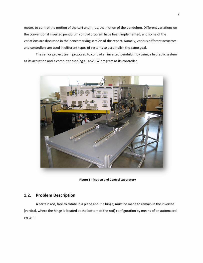
In the motion and control laboratory in Western Michigan University’s Parkview campus,
students learn how modern control theory can be applied to physical systems. Figure 1 is an example of
a hydraulic system that is ultimately controlled using a computer program to produce a certain desired
response of the sled attached to the hydraulic cylinder. Over the past 3 to 4 years, components of the
system shown in Figure 1 have been developed as senior projects building on the progress of other
senior projects. The current senior design team proposed another modification to the hydraulic sled by
introducing an inverted pendulum to the system.
In many college control engineering laboratories the classic inverted pendulum problem is
presented. A pendulum is a rod object that is hinged on one end of its length and is free to rotate about
the hinge. Often one encounters pendulums in clocks, where a rod hangs and swings from a joint at the
top of the rod. If the pendulum were inverted, the hinge would be located on the bottom of the rod. If
the rod length made a perfect right angle with the horizontal axis of the earth, the rod would remain
vertical. As soon as the rod angle changes, the rod would immediately rotate back to the non-inverted
configuration. However, if the hinge would move to prevent the pendulum from falling when the angle
changed, the pendulum angle could be maintained at about 90 degrees from the horizontal axis. A
person balancing a broomstick on his or her hand would be analogous to this system, except the hand is
replaced with some kind of mechanical actuation system. The hinge is typically fixed to a cart. An
electrical and computer system records positions as time progresses, using sensors, and calculate
appropriate input signals to the actuator. These signals would be used by an actuator, such as a DC
2
motor, to control the motion of the cart and, thus, the motion of the pendulum. Different variations on
the conventional inverted pendulum control problem have been implemented, and some of the
variations are discussed in the benchmarking section of the report. Namely, various different actuators
and controllers are used in different types of systems to accomplish the same goal.
The senior project team proposed to control an inverted pendulum by using a hydraulic system
as its actuation and a computer running a LabVIEW program as its controller.
Figure 1 - Motion and Control Laboratory
1.2. Problem Description
A certain rod, free to rotate in a plane about a hinge, must be made to remain in the inverted
(vertical, where the hinge is located at the bottom of the rod) configuration by means of an automated
system.
3
1.3. Need
As more demanding characteristics are being required of mechanical systems, better control of
the systems is also required. Furthermore, as systems in the future become more complicated to
perform more functions, future engineers need to have a better understanding of control systems and
control theory.
The proposed inverted pendulum system fits the need. The inverted pendulum control problem
is a solid starting point for testing different control algorithms on a physical system. Also, the inverted
pendulum system can easily be complicated further to test control algorithms on more complicated
systems. For instance, water can be placed in a jar at the top of the pendulum to introduce a
complicated disturbance. And, the inverted pendulum system will be used in the controls laboratory to
help future engineers graduating from Western Michigan University to better understand control of a
mechanical system.
1.4. Goal
The ultimate goal of the project was to produce a functioning inverted pendulum control system
for use in the motion and control laboratory at Western Michigan University. The senior project team
intended to present simulations of the system working, as well as the actual functioning product.
1.5. Impact
1.5.1. Environmental Impact
The inverted pendulum system itself poses a mild threat to the environment. The disposal of the
hydraulic fluid, if some fluid leaks from the system or needs to be replaced, requires attention. The
hydraulic filter requires proper disposal when replacement is necessary. Once the system is no longer
useful, proper care must be exercised in disposing of the parts. The environmental concern is mostly in
the electronics in the computer and sensors.
The development of improved control in mechanical systems has the potential to improve man’s
impact on the environment. Systems could be improved to better sort material waste in waste
management systems. Improved efficiency can be implemented in processes to reduce the usage of
energy. Increased safety in vehicles and machines can be implemented to avoid the amount waste
accumulated from vehicle collisions and destruction of machinery.

4
1.5.2. Global Impact
One global impact control technology has is in the area of the military. Advanced countries can
implement control techniques to bring soldiers out from the front lines of combat and replace them
with automated technology. This will change how a people or country thinks about war and can change
the decisions a country may make in that subject.
As communication and transportation brings the countries of the world closer together and
companies compete for markets from all around the globe, engineers and companies face competing in
a more demanding setting. As companies around the world utilize the most recent developments in
control system technology, engineers will be faced with the option of updating their understanding and
implementation of the technology or lose market share to competitors. Advances in control technology
are changing the way engineers are thinking about design around the world.
1.5.3. Impact on Society
Control theory has a large impact on society, because development in the area will change how
people live. For instance, control theory plays a major role in the progress of mechanization. As
companies begin to automate more procedures in manufacturing, jobs may be replaced with machines.
This will force people to take different kinds of jobs. Automation means people will be needed in
different areas, changing the kind of lives people live in the workplace. Control technology can affect the
lives of people in their homes as well, as daily processes at home can be become more automated by
“smart” products.
2. Requirements and Specifications
2.1. Functional Requirements
The functional requirements for the inverted pendulum must satisfy many areas for control
purposes and future upgrading/adjustments. This project is engineered for future demonstration
purposes also. Therefore, the user interface must be configured accordingly, being clear, informative,
and intuitive. The pendulum must be engineered for adjustability within bob weight and distance from
the pivot point. During operation the pendulum must maintain a range of plus or minus some angle for
vertical status.
5
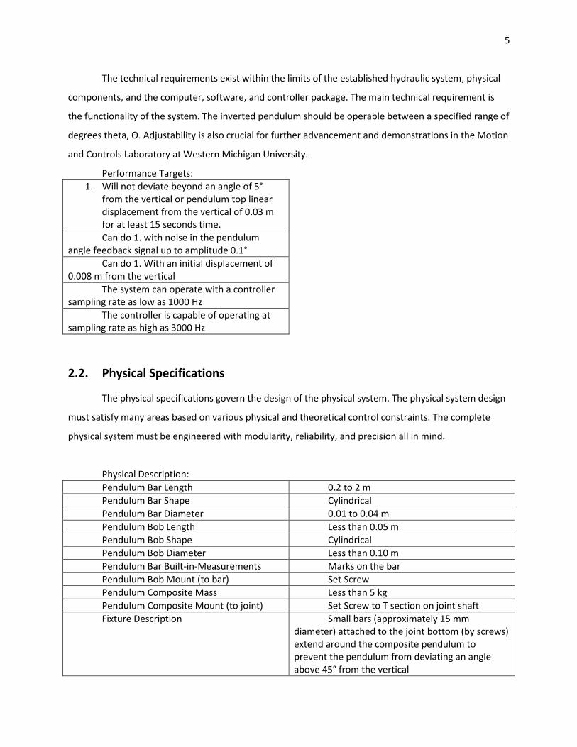
The technical requirements exist within the limits of the established hydraulic system, physical
components, and the computer, software, and controller package. The main technical requirement is
the functionality of the system. The inverted pendulum should be operable between a specified range of
degrees theta, Θ. Adjustability is also crucial for further advancement and demonstrations in the Motion
and Controls Laboratory at Western Michigan University.
Performance Targets:
1. Will not deviate beyond an angle of 5° from the vertical or pendulum top linear displacement from the vertical of 0.03 m for at least 15 seconds time.
Can do 1. with noise in the pendulum angle feedback signal up to amplitude 0.1°
Can do 1. With an initial displacement of 0.008 m from the vertical
The system can operate with a controller sampling rate as low as 1000 Hz
The controller is capable of operating at sampling rate as high as 3000 Hz
2.2. Physical Specifications
The physical specifications govern the design of the physical system. The physical system design
must satisfy many areas based on various physical and theoretical control constraints. The complete
physical system must be engineered with modularity, reliability, and precision all in mind.
Physical Description:
Pendulum Bar Length 0.2 to 2 m
Pendulum Bar Shape Cylindrical
Pendulum Bar Diameter 0.01 to 0.04 m
Pendulum Bob Length Less than 0.05 m
Pendulum Bob Shape Cylindrical
Pendulum Bob Diameter Less than 0.10 m
Pendulum Bar Built-in-Measurements Marks on the bar
Pendulum Bob Mount (to bar) Set Screw
Pendulum Composite Mass Less than 5 kg
Pendulum Composite Mount (to joint) Set Screw to T section on joint shaft
Fixture Description Small bars (approximately 15 mm diameter) attached to the joint bottom (by screws) extend around the composite pendulum to prevent the pendulum from deviating an angle above 45° from the vertical
6
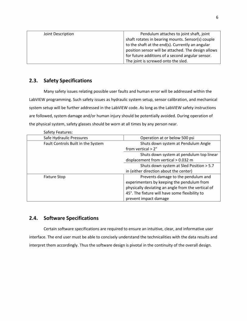
Joint Description Pendulum attaches to joint shaft, joint shaft rotates in bearing mounts. Sensor(s) couple to the shaft at the end(s). Currently an angular position sensor will be attached. The design allows for future additions of a second angular sensor. The joint is screwed onto the sled.
2.3. Safety Specifications
Many safety issues relating possible user faults and human error will be addressed within the
LabVIEW programming. Such safety issues as hydraulic system setup, sensor calibration, and mechanical
system setup will be further addressed in the LabVIEW code. As long as the LabVIEW safety instructions
are followed, system damage and/or human injury should be potentially avoided. During operation of
the physical system, safety glasses should be worn at all times by any person near.
Safety Features:
Safe Hydraulic Pressures Operation at or below 500 psi
Fault Controls Built in the System Shuts down system at Pendulum Angle from vertical > 2°
Shuts down system at pendulum top linear displacement from vertical > 0.032 m
Shuts down system at Sled Position > 5.7 in (either direction about the center)
Fixture Stop Prevents damage to the pendulum and experimenters by keeping the pendulum from physically deviating an angle from the vertical of 45°. The fixture will have some flexibility to prevent impact damage
2.4. Software Specifications
Certain software specifications are required to ensure an intuitive, clear, and informative user
interface. The end user must be able to concisely understand the technicalities with the data results and
interpret them accordingly. Thus the software design is pivotal in the continuity of the overall design.

7
Software Capabilities:
1. Simulates various models (linear, non-linear, with and without saturation effects) for the system using MATLAB/SIMULINK
2. Controls the system using a LABVIEW program
May Include:
1. Process for automatically recording and organizing input parameters
2. Tool(s) for automatic report generation of the results
3. Tool(s) for loading and creating calibration sets for systems that met or met some of the performance targets
4. Function of switching between control algorithms in the MATLAB/SIMULINK and LABVIEW programs
5. Integration of the MATLAB/SIMULINK and LABVIEW programs (allows one to calibrate, then simulate results, send the calibrations to LABVIEW automatically to run an experiment on the physical system)
6. Procedures and tools for allowing the system to calibrate itself for changes in the physical system
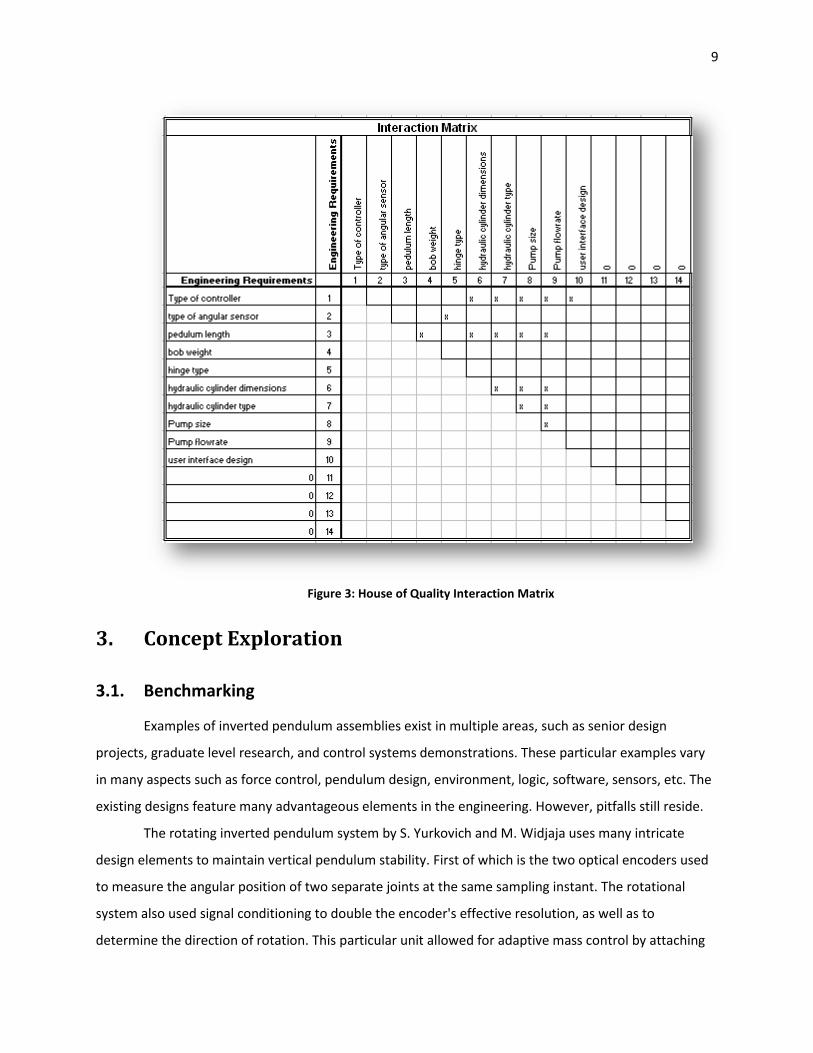
2.5. House of Quality and QFD
Requirements of the system as a whole demanded by the customer resulted in an interaction
matrix to aid in deciphering the importance of the engineering requirements. Thus prioritizing the
specifications of components and aspects of the design ultimately led to an optimized approach.
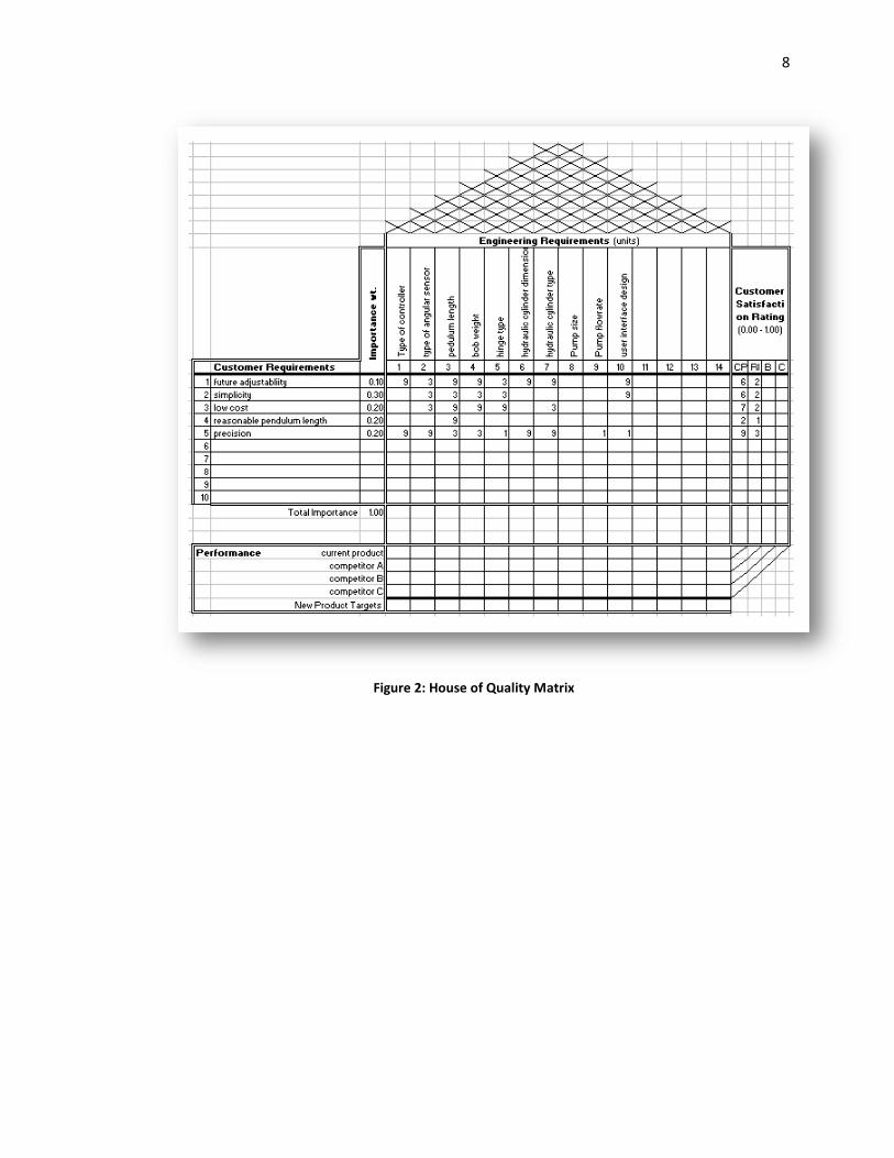
8
Figure 2: House of Quality Matrix
9
Figure 3: House of Quality Interaction Matrix
3. Concept Exploration
3.1. Benchmarking
Examples of inverted pendulum assemblies exist in multiple areas, such as senior design
projects, graduate level research, and control systems demonstrations. These particular examples vary
in many aspects such as force control, pendulum design, environment, logic, software, sensors, etc. The
existing designs feature many advantageous elements in the engineering. However, pitfalls still reside.
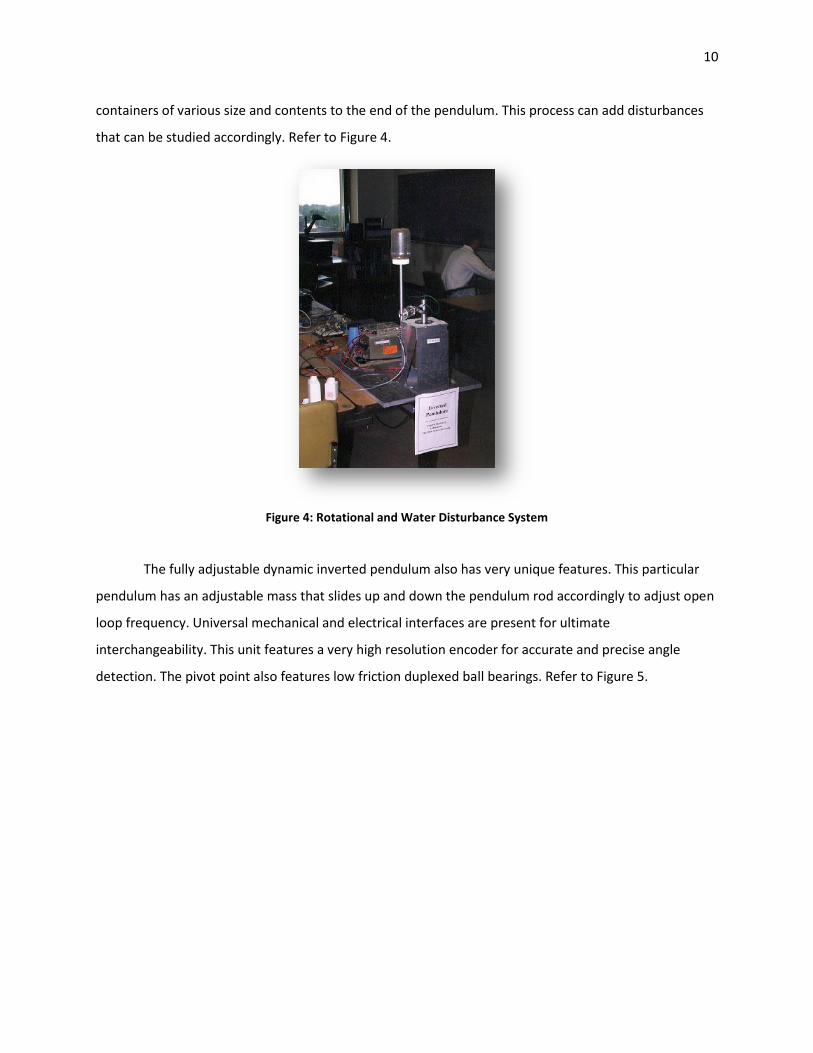
The rotating inverted pendulum system by S. Yurkovich and M. Widjaja uses many intricate
design elements to maintain vertical pendulum stability. First of which is the two optical encoders used
to measure the angular position of two separate joints at the same sampling instant. The rotational
system also used signal conditioning to double the encoder's effective resolution, as well as to
determine the direction of rotation. This particular unit allowed for adaptive mass control by attaching
10
containers of various size and contents to the end of the pendulum. This process can add disturbances
that can be studied accordingly. Refer to Figure 4.
Figure 4: Rotational and Water Disturbance System
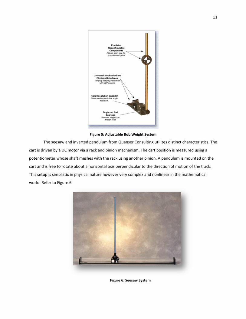
The fully adjustable dynamic inverted pendulum also has very unique features. This particular
pendulum has an adjustable mass that slides up and down the pendulum rod accordingly to adjust open
loop frequency. Universal mechanical and electrical interfaces are present for ultimate
interchangeability. This unit features a very high resolution encoder for accurate and precise angle
detection. The pivot point also features low friction duplexed ball bearings. Refer to Figure 5.
11
Figure 5: Adjustable Bob Weight System
The seesaw and inverted pendulum from Quanser Consulting utilizes distinct characteristics. The
cart is driven by a DC motor via a rack and pinion mechanism. The cart position is measured using a
potentiometer whose shaft meshes with the rack using another pinion. A pendulum is mounted on the
cart and is free to rotate about a horizontal axis perpendicular to the direction of motion of the track.
This setup is simplistic in physical nature however very complex and nonlinear in the mathematical
world. Refer to Figure 6.
Figure 6: Seesaw System
12
Pitfalls in Previous Designs:
Tilt Sensor:
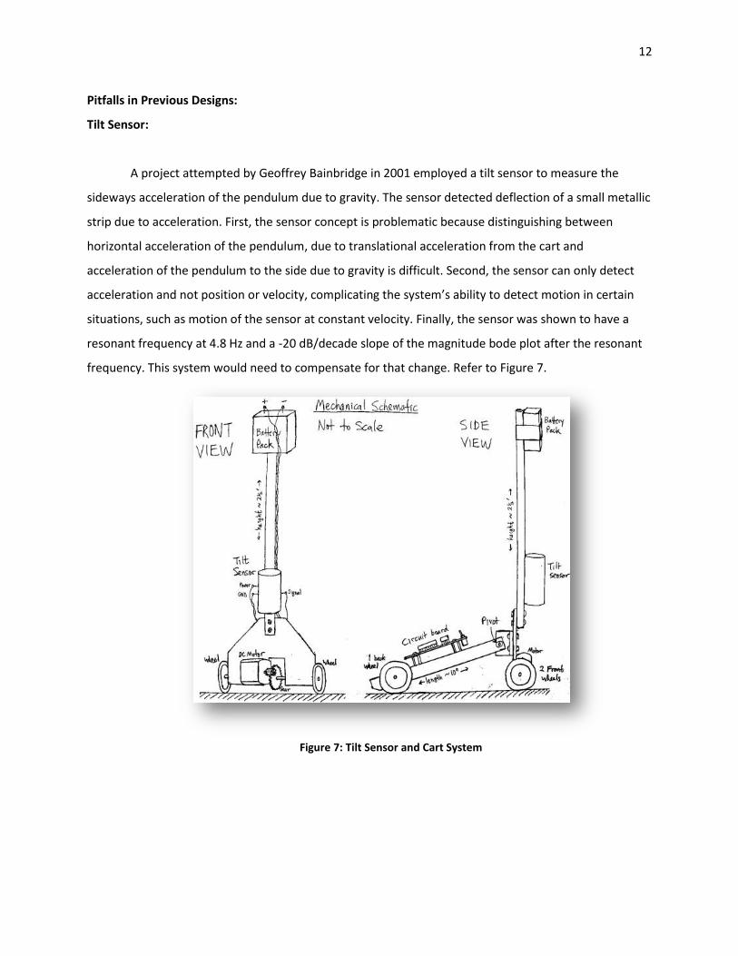
A project attempted by Geoffrey Bainbridge in 2001 employed a tilt sensor to measure the
sideways acceleration of the pendulum due to gravity. The sensor detected deflection of a small metallic
strip due to acceleration. First, the sensor concept is problematic because distinguishing between
horizontal acceleration of the pendulum, due to translational acceleration from the cart and
acceleration of the pendulum to the side due to gravity is difficult. Second, the sensor can only detect
acceleration and not position or velocity, complicating the system’s ability to detect motion in certain
situations, such as motion of the sensor at constant velocity. Finally, the sensor was shown to have a
resonant frequency at 4.8 Hz and a -20 dB/decade slope of the magnitude bode plot after the resonant
frequency. This system would need to compensate for that change. Refer to Figure 7.
Figure 7: Tilt Sensor and Cart System
13
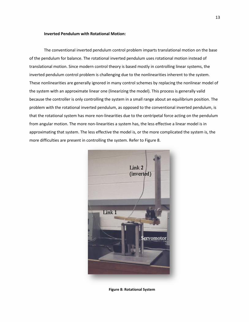
Inverted Pendulum with Rotational Motion:
The conventional inverted pendulum control problem imparts translational motion on the base
of the pendulum for balance. The rotational inverted pendulum uses rotational motion instead of
translational motion. Since modern control theory is based mostly in controlling linear systems, the
inverted pendulum control problem is challenging due to the nonlinearities inherent to the system.
These nonlinearities are generally ignored in many control schemes by replacing the nonlinear model of
the system with an approximate linear one (linearizing the model). This process is generally valid
because the controller is only controlling the system in a small range about an equilibrium position. The
problem with the rotational inverted pendulum, as opposed to the conventional inverted pendulum, is
that the rotational system has more non-linearities due to the centripetal force acting on the pendulum
from angular motion. The more non-linearities a system has, the less effective a linear model is in
approximating that system. The less effective the model is, or the more complicated the system is, the
more difficulties are present in controlling the system. Refer to Figure 8.
Figure 8: Rotational System
14
Seesaw and Inverted Pendulum System:
The conventional inverted pendulum is a two degree of freedom physical system. This means
only two equations of motion are required to describe the dynamics of the system: the angle of the
pendulum and the position of the cart. The see-saw system requires three equations of motion to
describe its dynamics: the angle of the pendulum, the position of the pendulum on the seesaw, and the
angle of the seesaw. This complicates further the control problem by requiring the controller to sense
more information about the system. Refer to Figure 6.
Benchmark conclusion:
These designs are all very unique, yet carry the same outcome of maintaining vertical pendulum
stability. Many norms are still present among the existing systems. The potentiometer is the sensor of
choice, usually for angular detection due to inexpensiveness and simplistic nature. Sticking with a single
axis (i.e. two degree of freedom system) for the forcing function maintains linearity for controlling the
system. Adjustable bob weight and mass location is extremely advantageous for adjustability of various
parameters. The existing designs for inverted pendulum systems are very useful for stemming new ideas
with the hydraulic actuated system.
3.2. Physical Decomposition
See flow diagrams in Function and Form Decomposition
3.3. Function Decomposition
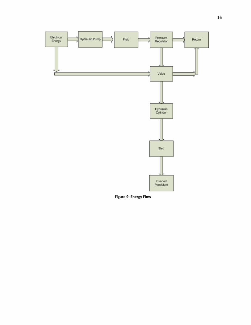
Overall Function: A system to control the angular position of an inverted pendulum
Energy flow
o Electrical energy is converted into mechanical energy in the work of a hydraulic pump.
o The mechanical energy in the pump is transmitted to the hydraulic fluid in the lines.
o Some of the energy in the fluid is bled off by the pressure regulator.
o Electrical energy is converted to mechanical energy in the valve.
o The valve position determines the energy flow in the hydraulic lines into the fluid return
or the hydraulic cylinder.
o The energy in the fluid is transmitted to mechanical energy in the hydraulic cylinder.
o The energy in the cylinder is transmitted to the sled.
o The energy in the sled is transmitted to the inverted pendulum.
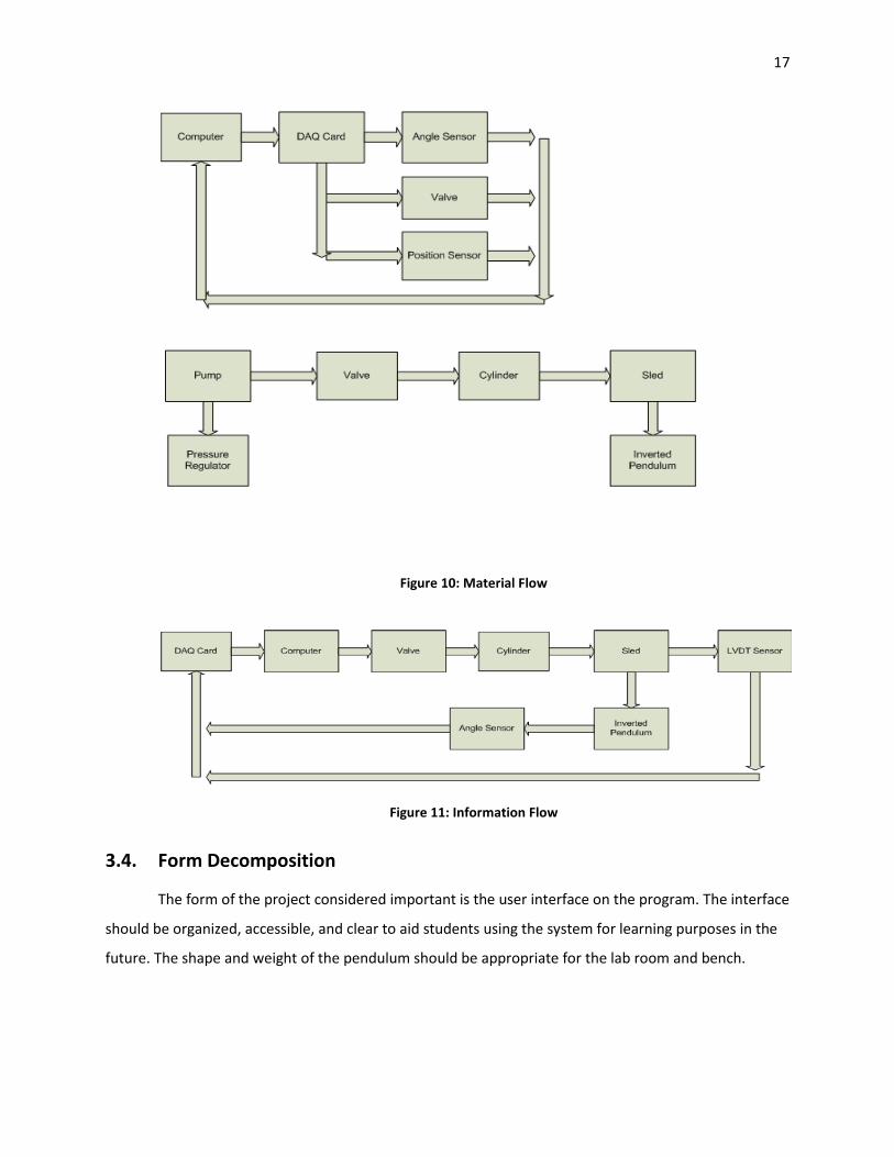
Material Flow
15
o Electric lines are connected to the pump and computer.
o The user interfaces with a computer running LabVIEW.
o The computer is connected to a DAQ card.
o The DAQ card is connected to the angle sensor, position sensor, and the valve.
o The pump is connected to hydraulic lines.
o The hydraulic lines are connected to a pressure regulator and the valve.
o The valve is connected to hydraulic lines to the hydraulic cylinder.
o The cylinder is connected to a sled.
o The sled moves on two tracks on a bench.
o The position sensor is attached to the bench.
o A fixture is attached to the sled.
o The fixture is attached to the angle sensor, pendulum stop, and pendulum hinge.
o The hinge is connected to the inverted pendulum.
Information Flow
o The desired change in angular position information is set in the LabVIEW program (Δθ =
0 ideally) on the computer.
o The computer sends necessary electrical information to a DAQ card.
o The DAQ card sends a voltage signal to a valve.
o The valve position information directs the flow direction and rate in the hydraulic lines.
o The pressure drop across the piston in the hydraulic cylinder is a result of the flow
direction and rate in the lines.
o The differential pressure determines the motion of the cylinder.
o The motion of the cylinder determines the motion of the sled.
o The position information of the sled is collected by a linear variable differential
transformer and sent back to the DAQ card.
o The motion of the sled determines the angle of the inverted pendulum.
o The angular position information of the inverted pendulum is collected by an angular
sensor and sent back to the DAQ card.
o The DAQ card sends a signal to the computer and program.
o The program calculates new electrical signals to be sent back to the DAQ card.
16
Figure 9: Energy Flow
17
Figure 10: Material Flow
Figure 11: Information Flow
3.4. Form Decomposition
The form of the project considered important is the user interface on the program. The interface
should be organized, accessible, and clear to aid students using the system for learning purposes in the
future. The shape and weight of the pendulum should be appropriate for the lab room and bench.
18
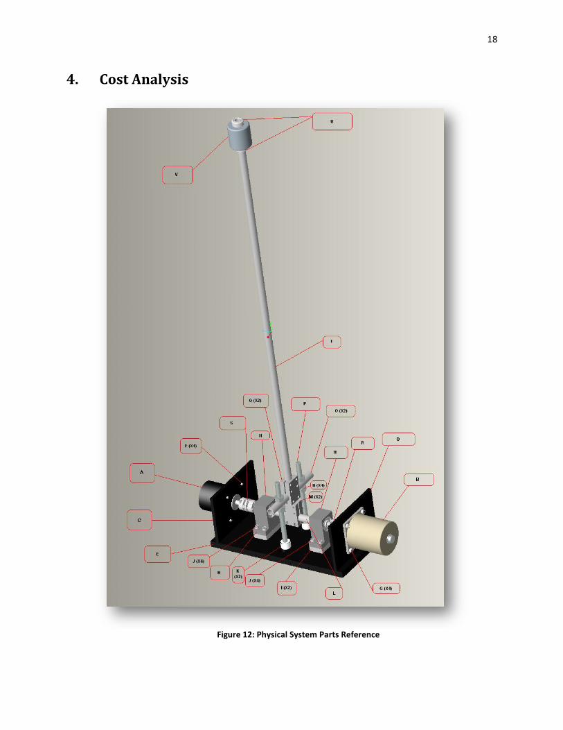
4. Cost Analysis
Figure 12: Physical System Parts Reference
19
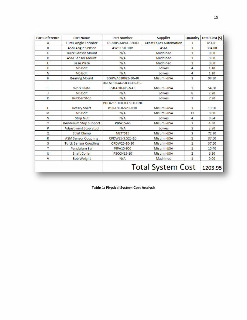
Table 1: Physical System Cost Analysis
20
5. Project Schedule
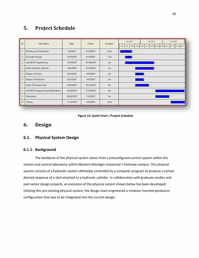
Figure 13: Gantt Chart / Project Schedule
6. Design
6.1. Physical System Design
6.1.1. Background
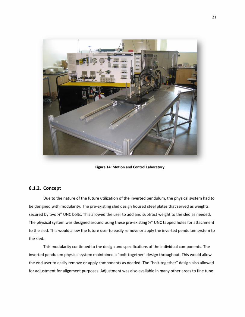
The backbone of the physical system stems from a preconfigured control system within the
motion and control laboratory within Western Michigan University’s Parkview campus. This physical
system consists of a hydraulic system ultimately controlled by a computer program to produce a certain
desired response of a sled attached to a hydraulic cylinder. In collaboration with graduate studies and
past senior design projects, an evolution of the physical system shown below has been developed.
Utilizing this pre-existing physical system, the design team engineered a modular inverted pendulum
configuration that was to be integrated into the current design.
21
Figure 14: Motion and Control Laboratory
6.1.2. Concept
Due to the nature of the future utilization of the inverted pendulum, the physical system had to
be designed with modularity. The pre-existing sled design housed steel plates that served as weights
secured by two ½” UNC bolts. This allowed the user to add and subtract weight to the sled as needed.
The physical system was designed around using these pre-existing ½” UNC tapped holes for attachment
to the sled. This would allow the future user to easily remove or apply the inverted pendulum system to
the sled.
This modularity continued to the design and specifications of the individual components. The
inverted pendulum physical system maintained a “bolt-together” design throughout. This would allow
the end user to easily remove or apply components as needed. The “bolt-together” design also allowed
for adjustment for alignment purposes. Adjustment was also available in many other areas to fine tune
22
the physical system in conjunction with the control system. These adjustable parameters include: bob
weight linear position, pendulum stop angle, sensor alignment, etc.
The physical system was designed to incorporate both analog and digital sensors. The design
team chose the latter, however the physical system accommodated both sensors to be attached
simultaneously. This allowed for future experiments for comparing the effects of analog vs. digital
sensors.
Lastly the inverted pendulum physical system was design with reliability and precision in mind.
The physical system will be used for many semesters to come, therefore reliability was crucial. All
components were designed and specified for robustness and future adaptability for such parameters as:
bob and physical system weight, pendulum length and material, sensor precision, etc. The physical
system could not exhibit “slop” in the conjunction of pendulum position and sensor output. This was
pivotal for the accuracy and recovery of the control system.
6.1.2.1. Custom Configurable Parts
Aside from general machining and fabrication, most of the components within the physical
system were designed and ordered in conjunction with Misumi USA Inc. Misumi USA Inc. is a subsidiary
of the Japan-based Misumi Corporation, which is the world’s largest supplier of configurable
components for assembly automation. Misumi provides the resources to custom configure over 600,000
unique components manufactured in both Metric and US units. Turn-around time is a crucial component
to achieving a project’s outcome. All components ordered from Misumi arrived within a one week
bracket minimizing build down time. They are also easily configured using their interactive online
resources. Their catalog is online in PDF format for easy reference and parts can be configured and
viewed utilizing Misumi’s 3D CAD preview. Price quotes are also automated resulting in an incredibly
fast turn-around time as well. For ordering information or future reference, visit www.misumiusa.com.
6.1.3. Proposed Configuration
6.1.3.1. Pendulum Design
The pendulum was designed around a few key physical system specifications. Again, the general
recurring theme for the physical system design is modularity. The pendulum bar shape was chosen to be
cylindrical for adjustability and symmetry. The bar’s length was deemed appropriate in the range of
23
0.2m to 2m in total length. Likewise, the bar’s overall diameter needed to reside within the 0.01m to
0.04m bracket.
The bob weight was designed in conjunction with the pendulum. Thus the bob weight was
required to be cylindrical in shape and less than 0.10m in diameter and 0.05m in overall length. With a
hole bored out in the center of the cylinder, the bob could easily be adjusted vertically up or down the
pendulum bar. To secure the bob weight to the cylinder shaft collars would be required to hold the bob
in place on both the top and bottom sides.
6.1.3.1.1. Components and Materials
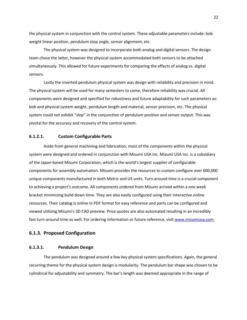
The pendulum bar was specified as 6063 Aluminum. This particular version of Aluminum allows
for a low-cost, light-weight, yet strong option to sustain the forces exhibited within the system. The bar
was also a thin walled version which is again a lower cost due to the drawn manufacturing processes.
Selecting the bar in Aluminum also allows for more adjustability with weight fluctuation. By initially
starting with less overall weight in the bar, the user can add more weight to the bob or slide the bob
weight up or down to adjust the moment of inertia. If the bar were made of steel, initial weight could
not be taken away and would slow down the system.
Figure 15: PIPA15-900 Pendulum Bar
24
The bob weight was a custom machined piece made from low carbon solid stock steel. The steel
material of the bob weight allowed for a large amount of weight in a compact space due to steel’s
higher relative density. Starting with a rough 2in length of 1.75in solid round stock cut on the band saw,
the bob weight was turned on the lathe to the desired 1.875in and edges were chamfered to ease
handling. Lastly the bob weight was bored out, again on the lathe, to slightly over the diameter of the
pendulum bar. This would ensure smooth travel during adjustment operations.
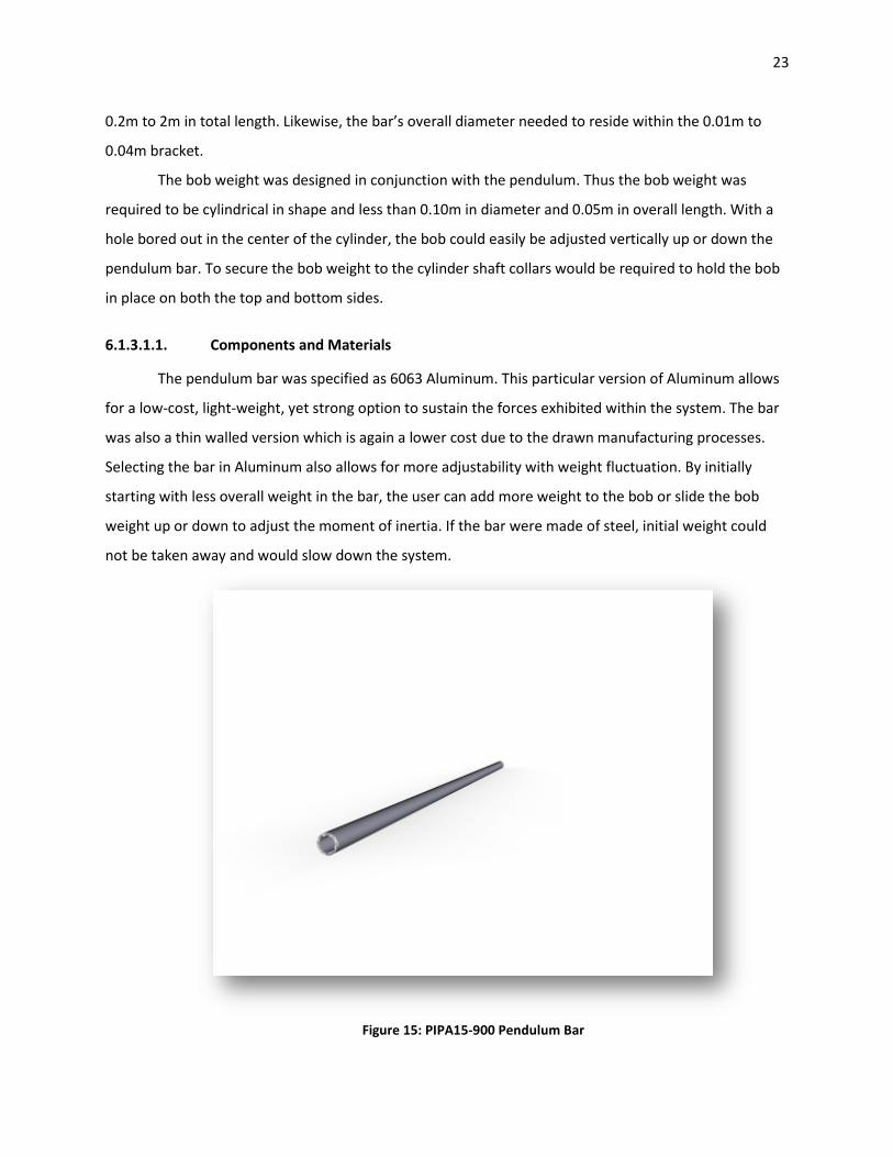
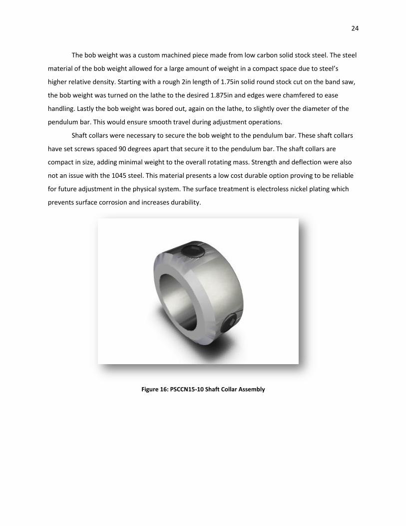
Shaft collars were necessary to secure the bob weight to the pendulum bar. These shaft collars
have set screws spaced 90 degrees apart that secure it to the pendulum bar. The shaft collars are
compact in size, adding minimal weight to the overall rotating mass. Strength and deflection were also
not an issue with the 1045 steel. This material presents a low cost durable option proving to be reliable
for future adjustment in the physical system. The surface treatment is electroless nickel plating which
prevents surface corrosion and increases durability.
Figure 16: PSCCN15-10 Shaft Collar Assembly
25
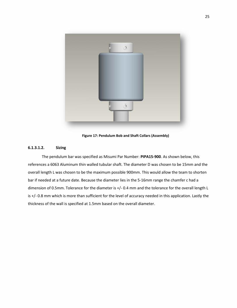
Figure 17: Pendulum Bob and Shaft Collars (Assembly)
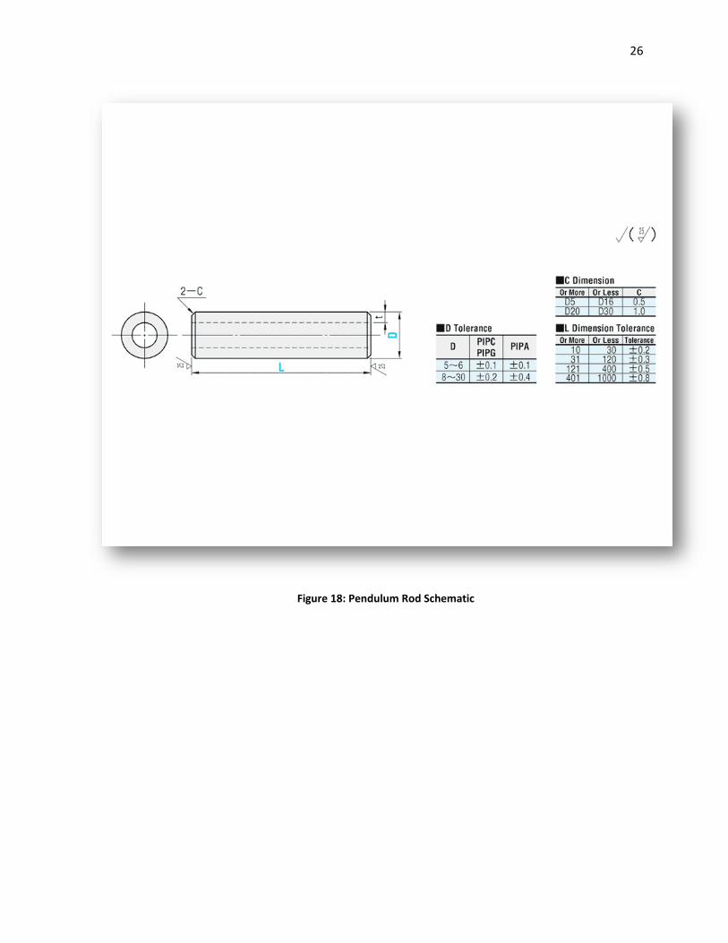
6.1.3.1.2. Sizing
The pendulum bar was specified as Misumi Par Number: PIPA15-900. As shown below, this
references a 6063 Aluminum thin walled tubular shaft. The diameter D was chosen to be 15mm and the
overall length L was chosen to be the maximum possible 900mm. This would allow the team to shorten
bar if needed at a future date. Because the diameter lies in the 5-16mm range the chamfer c had a
dimension of 0.5mm. Tolerance for the diameter is +/- 0.4 mm and the tolerance for the overall length L
is +/- 0.8 mm which is more than sufficient for the level of accuracy needed in this application. Lastly the
thickness of the wall is specified at 1.5mm based on the overall diameter.
26
Figure 18: Pendulum Rod Schematic
27
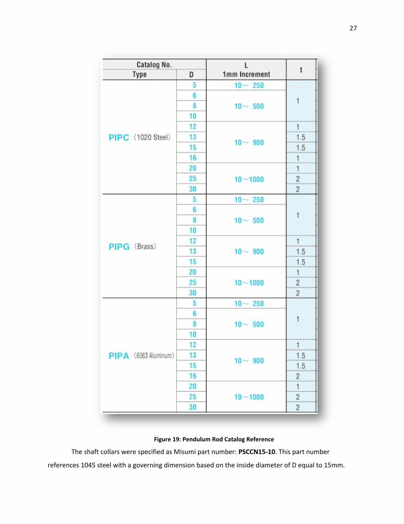
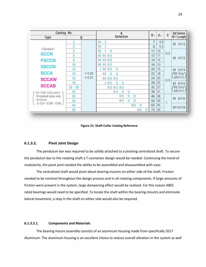
Figure 19: Pendulum Rod Catalog Reference
The shaft collars were specified as Misumi part number: PSCCN15-10. This part number
references 1045 steel with a governing dimension based on the inside diameter of D equal to 15mm.
28
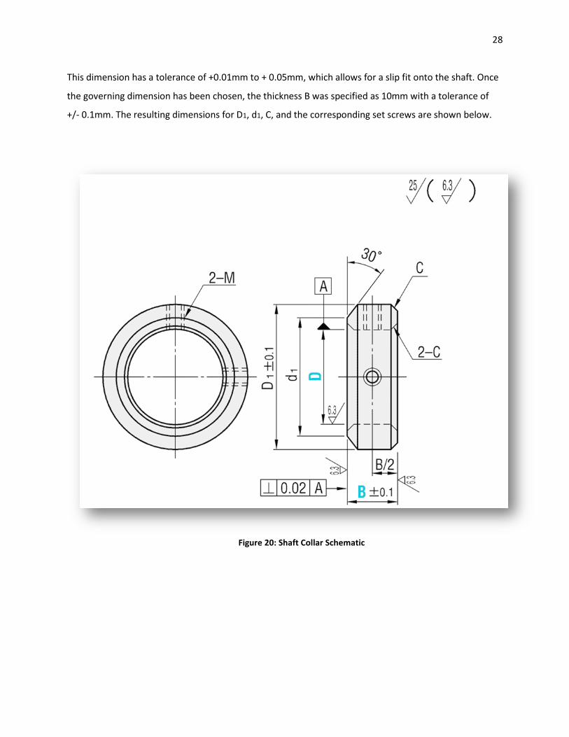
This dimension has a tolerance of +0.01mm to + 0.05mm, which allows for a slip fit onto the shaft. Once
the governing dimension has been chosen, the thickness B was specified as 10mm with a tolerance of
+/- 0.1mm. The resulting dimensions for D1, d1, C, and the corresponding set screws are shown below.
Figure 20: Shaft Collar Schematic
29
Figure 21: Shaft Collar Catalog Reference
6.1.3.2. Pivot Joint Design
The pendulum bar was required to be solidly attached to a pivoting centralized shaft. To secure
the pendulum bar to the rotating shaft a T-connector design would be needed. Continuing the trend of
modularity, the pivot joint needed the ability to be assembled and disassembled with ease.
The centralized shaft would pivot about bearing mounts on either side of the shaft. Friction
needed to be minimal throughout the design process and in all rotating components. If large amounts of
friction were present in the system, large dampening effect would be realized. For this reason ABEC
rated bearings would need to be specified. To locate the shaft within the bearing mounts and eliminate
lateral movement, a step in the shaft on either side would also be required.
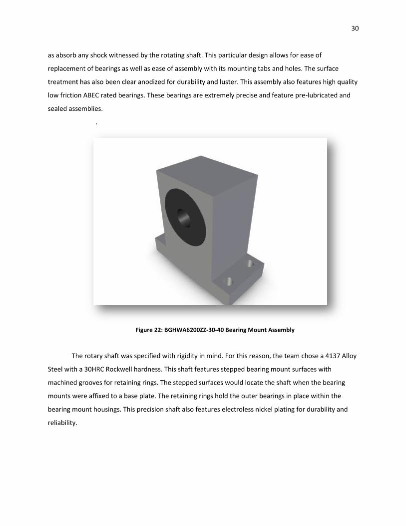
6.1.3.2.1. Components and Materials
The bearing mount assembly consists of an aluminum housing made from specifically 2017
Aluminum. The aluminum housing is an excellent choice to reduce overall vibration in the system as well
30
as absorb any shock witnessed by the rotating shaft. This particular design allows for ease of
replacement of bearings as well as ease of assembly with its mounting tabs and holes. The surface
treatment has also been clear anodized for durability and luster. This assembly also features high quality
low friction ABEC rated bearings. These bearings are extremely precise and feature pre-lubricated and
sealed assemblies.
.
Figure 22: BGHWA6200ZZ-30-40 Bearing Mount Assembly
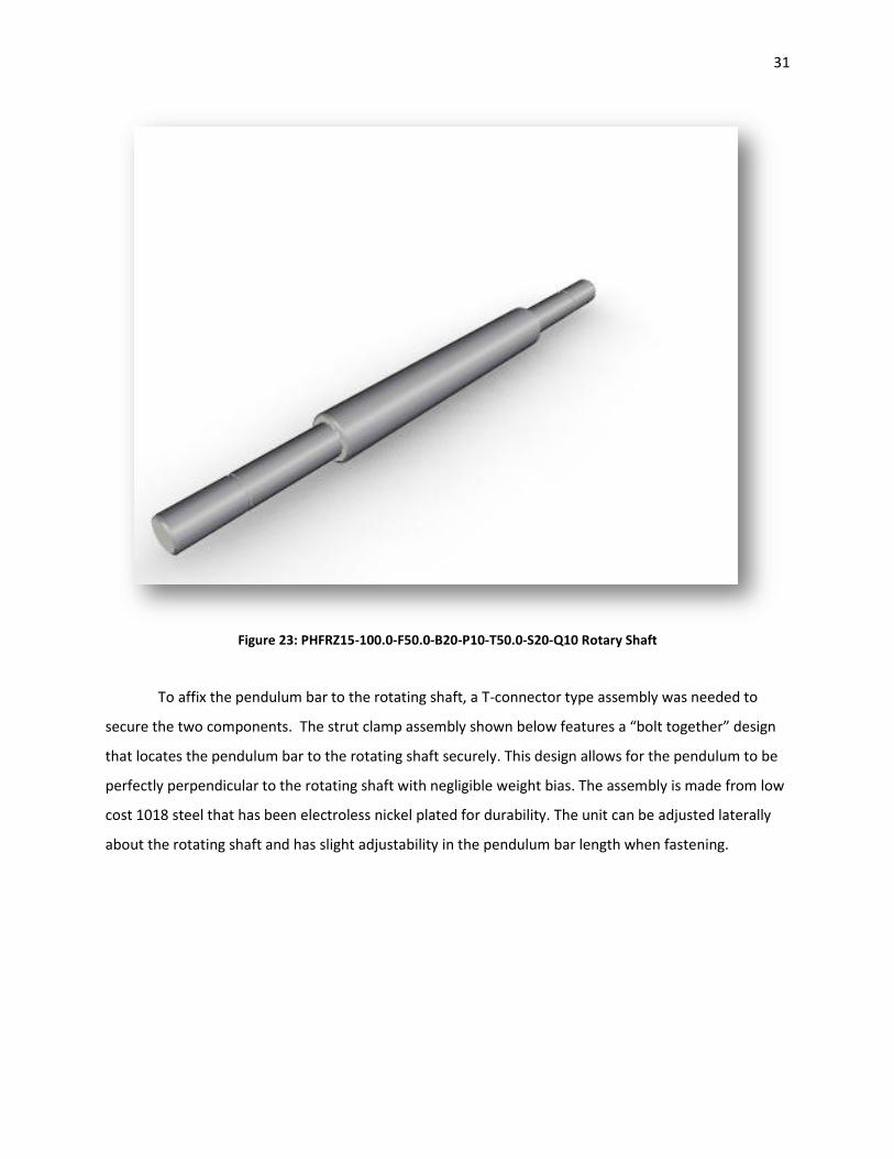
The rotary shaft was specified with rigidity in mind. For this reason, the team chose a 4137 Alloy
Steel with a 30HRC Rockwell hardness. This shaft features stepped bearing mount surfaces with
machined grooves for retaining rings. The stepped surfaces would locate the shaft when the bearing
mounts were affixed to a base plate. The retaining rings hold the outer bearings in place within the
bearing mount housings. This precision shaft also features electroless nickel plating for durability and
reliability.
31
Figure 23: PHFRZ15-100.0-F50.0-B20-P10-T50.0-S20-Q10 Rotary Shaft
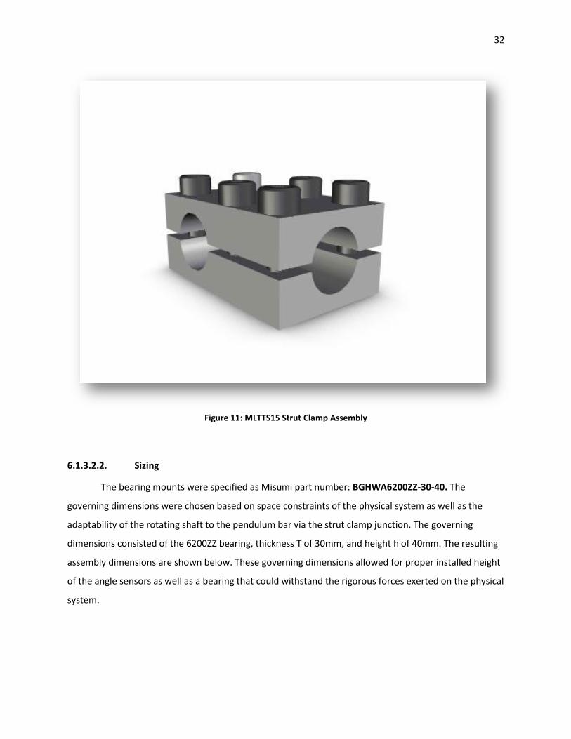
To affix the pendulum bar to the rotating shaft, a T-connector type assembly was needed to
secure the two components. The strut clamp assembly shown below features a “bolt together” design
that locates the pendulum bar to the rotating shaft securely. This design allows for the pendulum to be
perfectly perpendicular to the rotating shaft with negligible weight bias. The assembly is made from low
cost 1018 steel that has been electroless nickel plated for durability. The unit can be adjusted laterally
about the rotating shaft and has slight adjustability in the pendulum bar length when fastening.
32
Figure 11: MLTTS15 Strut Clamp Assembly
6.1.3.2.2. Sizing
The bearing mounts were specified as Misumi part number: BGHWA6200ZZ-30-40. The
governing dimensions were chosen based on space constraints of the physical system as well as the
adaptability of the rotating shaft to the pendulum bar via the strut clamp junction. The governing
dimensions consisted of the 6200ZZ bearing, thickness T of 30mm, and height h of 40mm. The resulting
assembly dimensions are shown below. These governing dimensions allowed for proper installed height
of the angle sensors as well as a bearing that could withstand the rigorous forces exerted on the physical
system.
33
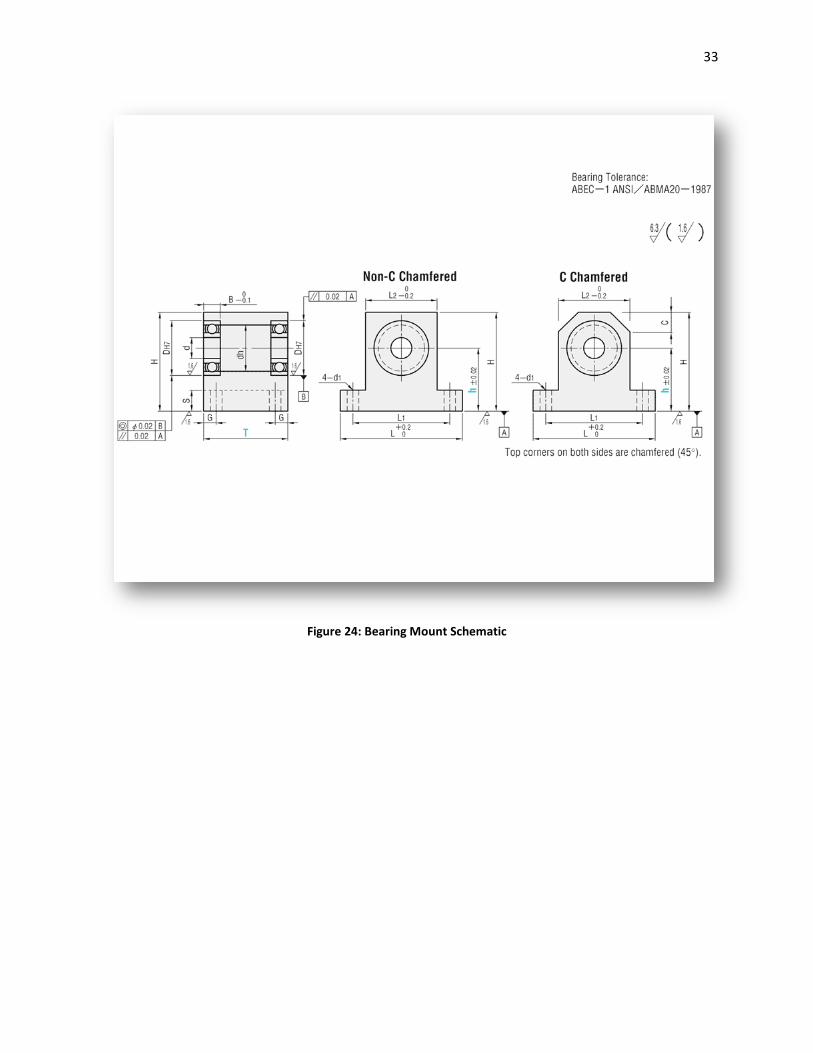
Figure 24: Bearing Mount Schematic
34
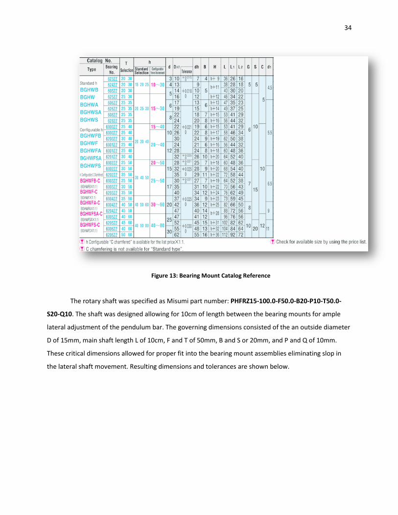
Figure 13: Bearing Mount Catalog Reference
The rotary shaft was specified as Misumi part number: PHFRZ15-100.0-F50.0-B20-P10-T50.0-
S20-Q10. The shaft was designed allowing for 10cm of length between the bearing mounts for ample
lateral adjustment of the pendulum bar. The governing dimensions consisted of the an outside diameter
D of 15mm, main shaft length L of 10cm, F and T of 50mm, B and S or 20mm, and P and Q of 10mm.
These critical dimensions allowed for proper fit into the bearing mount assemblies eliminating slop in
the lateral shaft movement. Resulting dimensions and tolerances are shown below.
35
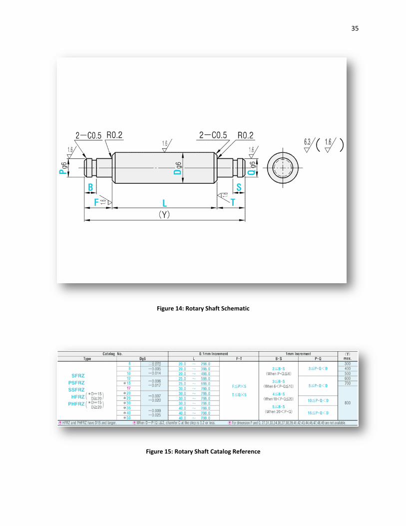
Figure 14: Rotary Shaft Schematic
Figure 15: Rotary Shaft Catalog Reference
36
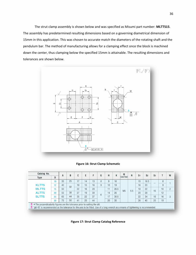
The strut clamp assembly is shown below and was specified as Misumi part number: MLTTS15.
The assembly has predetermined resulting dimensions based on a governing diametrical dimension of
15mm in this application. This was chosen to accurate match the diameters of the rotating shaft and the
pendulum bar. The method of manufacturing allows for a clamping effect once the block is machined
down the center, thus clamping below the specified 15mm is attainable. The resulting dimensions and
tolerances are shown below.
Figure 16: Strut Clamp Schematic
Figure 17: Strut Clamp Catalog Reference
37
6.1.3.3. Fixture Design
Once the pendulum design and pivot joint design were complete, the physical system needed a
platform and foundation to allow ease of application and removal from the sled, a reliable sensor
mounting and junction system, and a pendulum stop system. The overall fixture design required the
allowing for future additions of angle sensors as well as the sensors to couple at the ends of the rotating
shaft. The continuity of modularity was also required to ease the assembly and disassembly processes.
6.1.3.3.1. Components and Materials
To couple the main angle encoder as well as a future analog sensor, flexible sensor couplings as
shown below were specified. The units are originally intended for servo motor shaft coupling which
demands torsional rigidity, yet also requires flexibility for shaft misalignment. The sensor couplings are a
double disk design machined from lightweight aluminum which adds negligible dampening effect to the
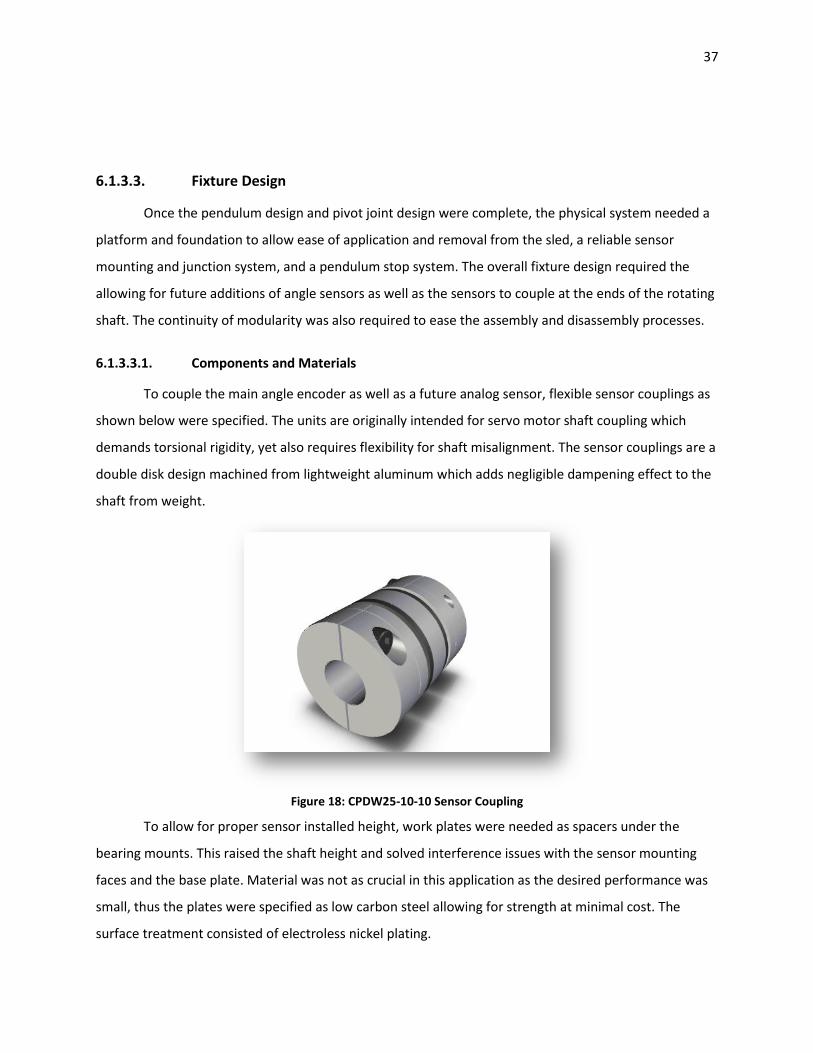
shaft from weight.
Figure 18: CPDW25-10-10 Sensor Coupling
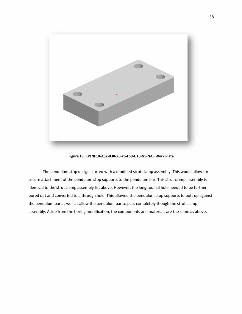
To allow for proper sensor installed height, work plates were needed as spacers under the
bearing mounts. This raised the shaft height and solved interference issues with the sensor mounting
faces and the base plate. Material was not as crucial in this application as the desired performance was
small, thus the plates were specified as low carbon steel allowing for strength at minimal cost. The
surface treatment consisted of electroless nickel plating.
38
Figure 19: KPLNF10-A62-B30-X6-Y6-F50-G18-N5-NA5 Work Plate
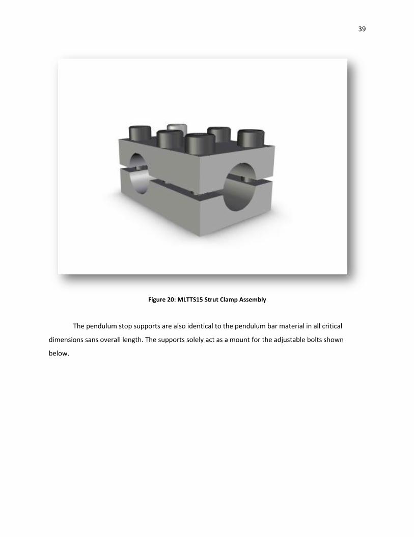
The pendulum stop design started with a modified strut clamp assembly. This would allow for
secure attachment of the pendulum stop supports to the pendulum bar. This strut clamp assembly is
identical to the strut clamp assembly list above. However, the longitudinal hole needed to be further
bored out and converted to a through hole. This allowed the pendulum stop supports to butt up against
the pendulum bar as well as allow the pendulum bar to pass completely though the strut clamp
assembly. Aside from the boring modification, the components and materials are the same as above.
39
Figure 20: MLTTS15 Strut Clamp Assembly
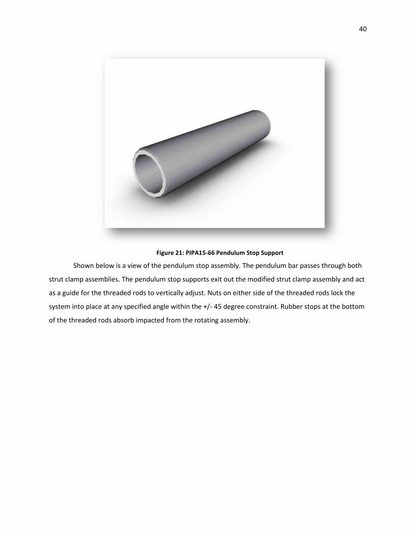
The pendulum stop supports are also identical to the pendulum bar material in all critical
dimensions sans overall length. The supports solely act as a mount for the adjustable bolts shown
below.
40
Figure 21: PIPA15-66 Pendulum Stop Support
Shown below is a view of the pendulum stop assembly. The pendulum bar passes through both
strut clamp assemblies. The pendulum stop supports exit out the modified strut clamp assembly and act
as a guide for the threaded rods to vertically adjust. Nuts on either side of the threaded rods lock the
system into place at any specified angle within the +/- 45 degree constraint. Rubber stops at the bottom
of the threaded rods absorb impacted from the rotating assembly.
41
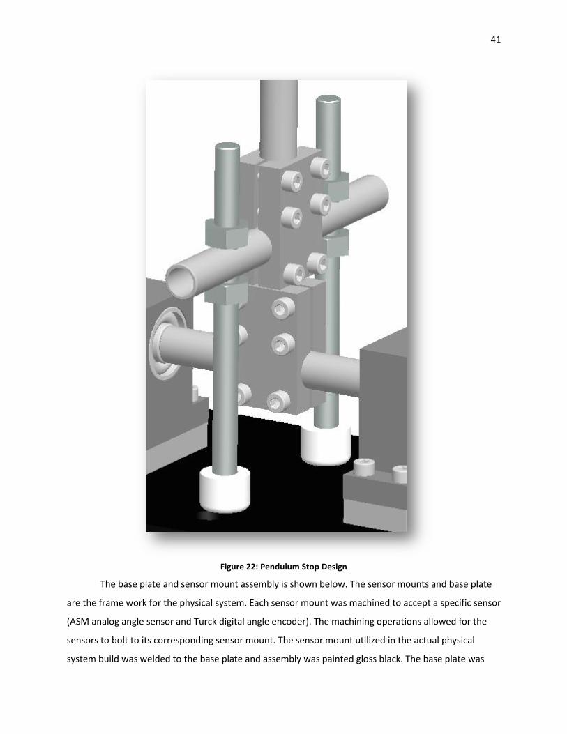
Figure 22: Pendulum Stop Design
The base plate and sensor mount assembly is shown below. The sensor mounts and base plate
are the frame work for the physical system. Each sensor mount was machined to accept a specific sensor
(ASM analog angle sensor and Turck digital angle encoder). The machining operations allowed for the
sensors to bolt to its corresponding sensor mount. The sensor mount utilized in the actual physical
system build was welded to the base plate and assembly was painted gloss black. The base plate was
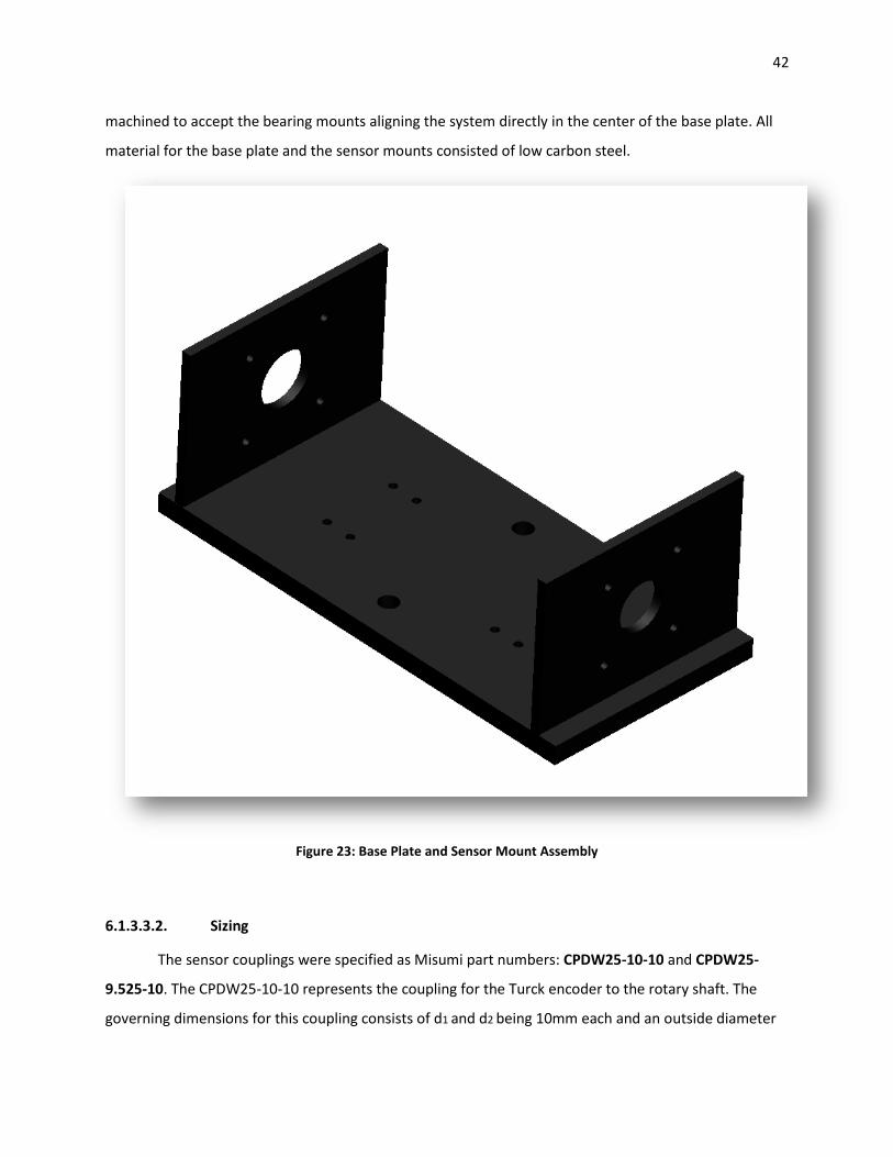
42
machined to accept the bearing mounts aligning the system directly in the center of the base plate. All
material for the base plate and the sensor mounts consisted of low carbon steel.
Figure 23: Base Plate and Sensor Mount Assembly
6.1.3.3.2. Sizing
The sensor couplings were specified as Misumi part numbers: CPDW25-10-10 and CPDW25-
9.525-10. The CPDW25-10-10 represents the coupling for the Turck encoder to the rotary shaft. The
governing dimensions for this coupling consists of d1 and d2 being 10mm each and an outside diameter
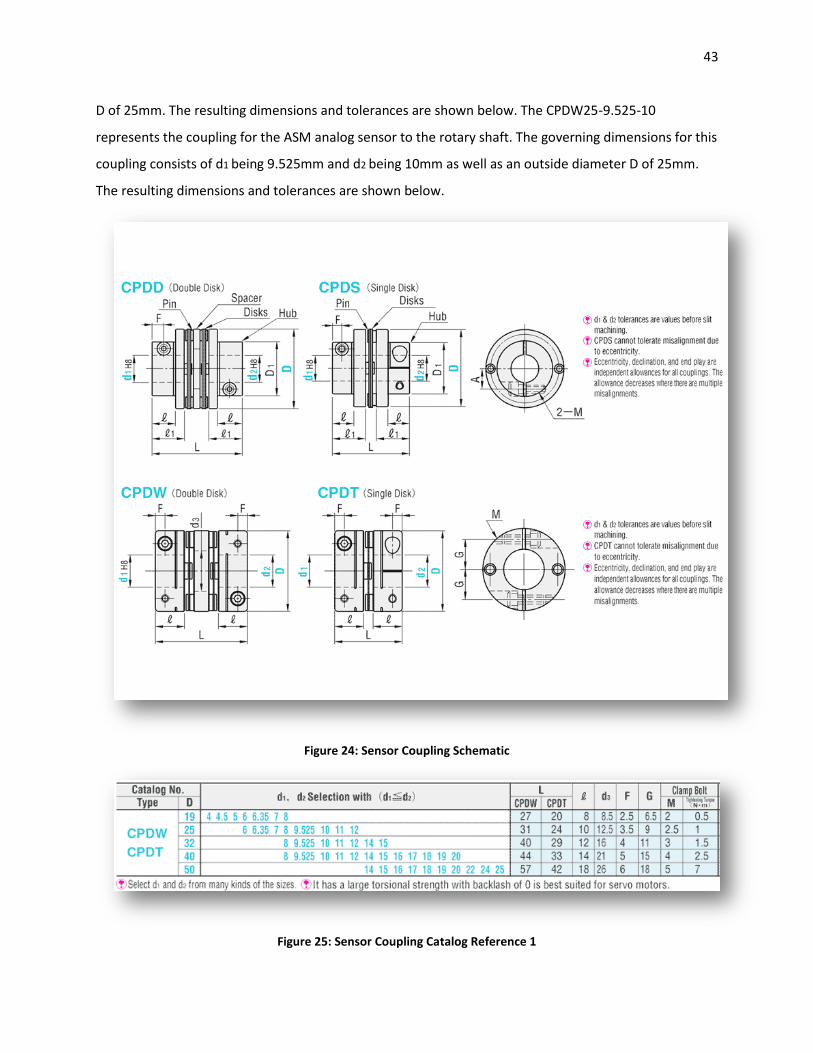
43
D of 25mm. The resulting dimensions and tolerances are shown below. The CPDW25-9.525-10
represents the coupling for the ASM analog sensor to the rotary shaft. The governing dimensions for this
coupling consists of d1 being 9.525mm and d2 being 10mm as well as an outside diameter D of 25mm.
The resulting dimensions and tolerances are shown below.
Figure 24: Sensor Coupling Schematic
Figure 25: Sensor Coupling Catalog Reference 1
44
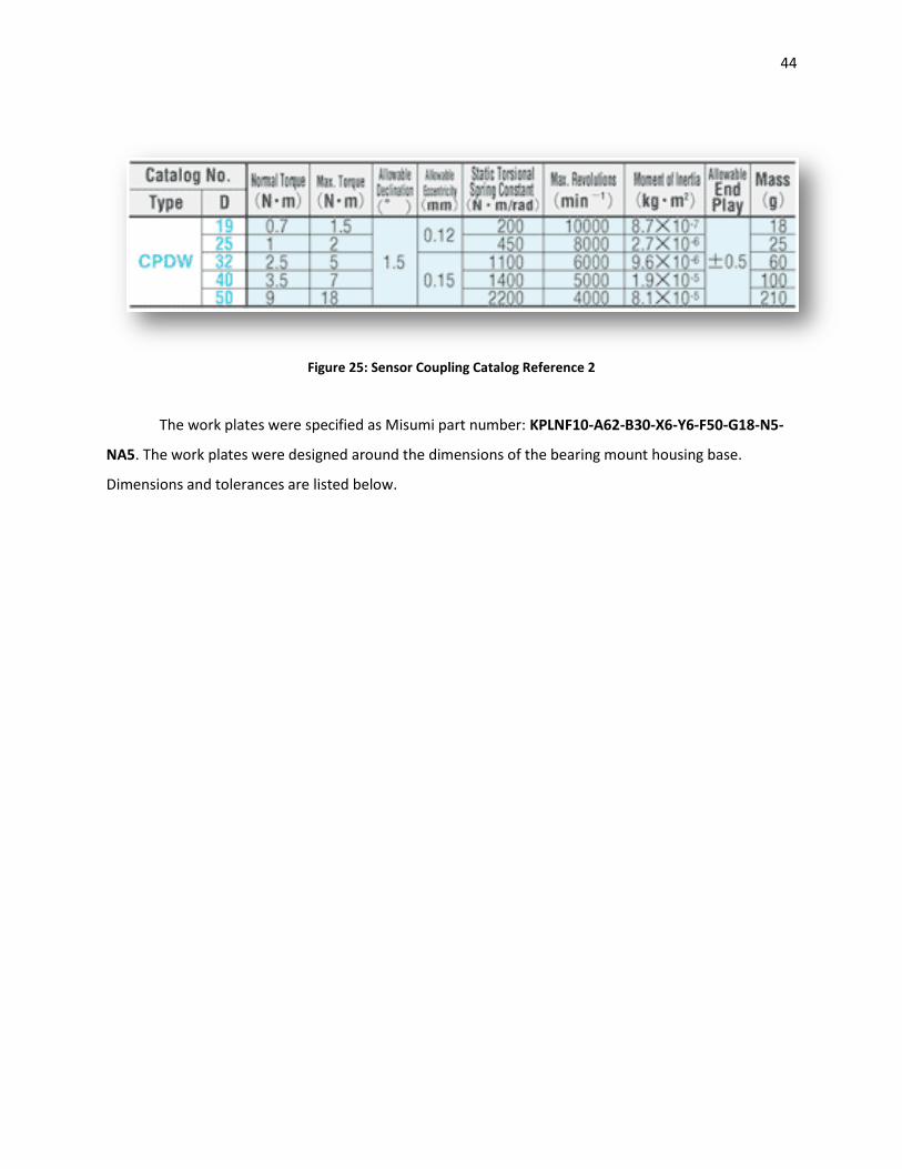
Figure 25: Sensor Coupling Catalog Reference 2
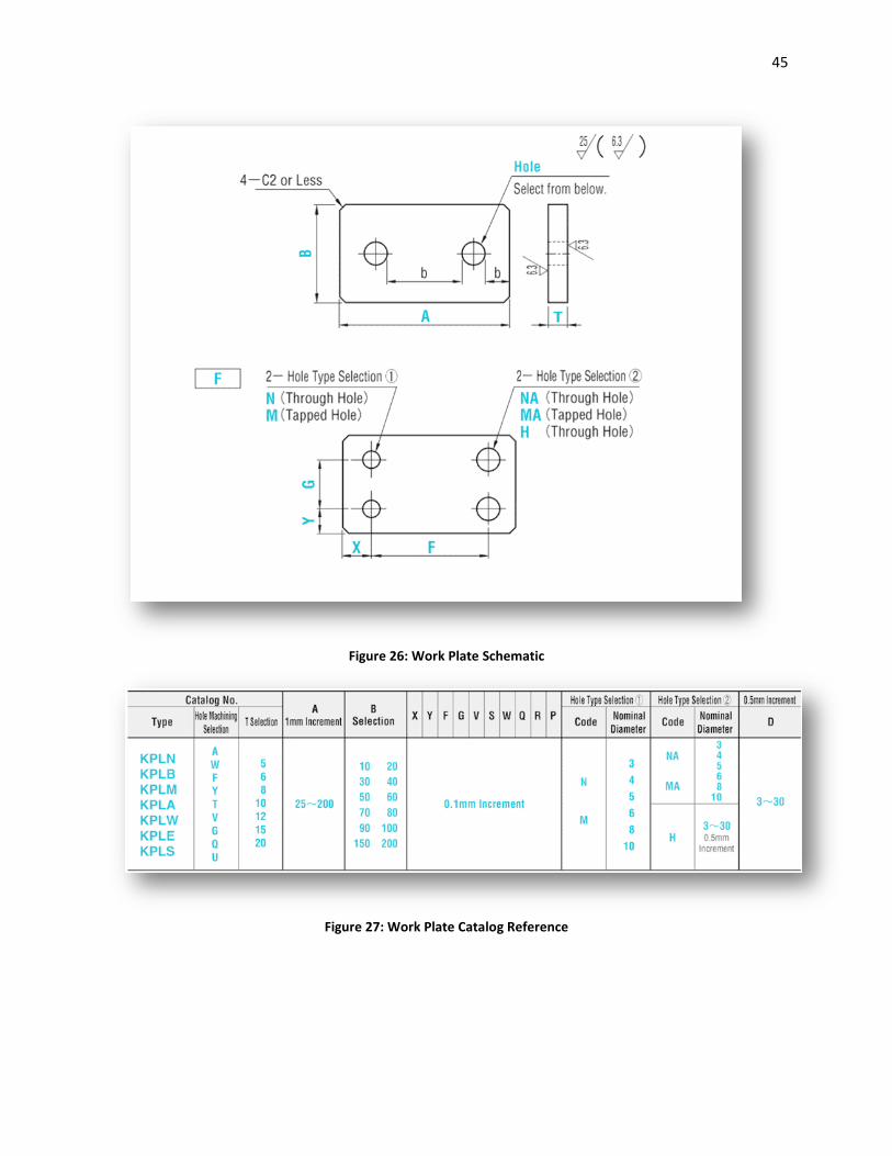
The work plates were specified as Misumi part number: KPLNF10-A62-B30-X6-Y6-F50-G18-N5-
NA5. The work plates were designed around the dimensions of the bearing mount housing base.
Dimensions and tolerances are listed below.
45
Figure 26: Work Plate Schematic
Figure 27: Work Plate Catalog Reference
46
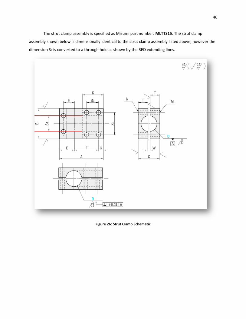
The strut clamp assembly is specified as Misumi part number: MLTTS15. The strut clamp
assembly shown below is dimensionally identical to the strut clamp assembly listed above; however the
dimension S1 is converted to a through hole as shown by the RED extending lines.
Figure 26: Strut Clamp Schematic
47
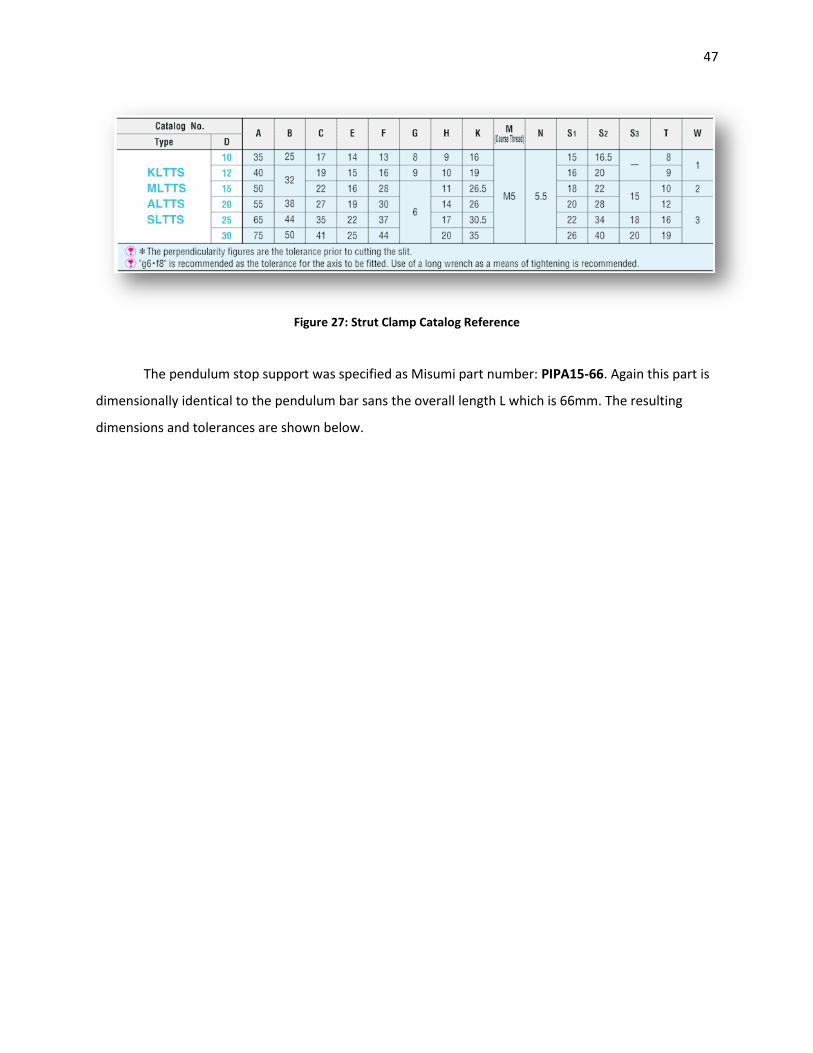
Figure 27: Strut Clamp Catalog Reference
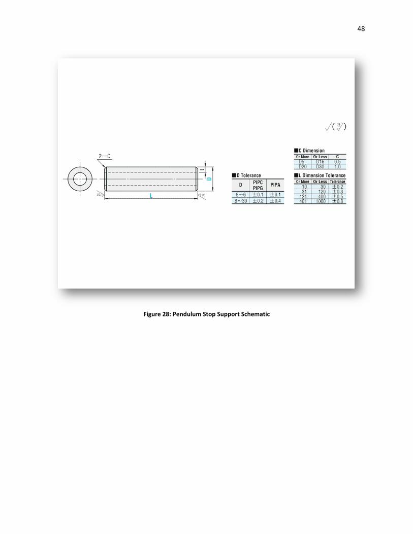
The pendulum stop support was specified as Misumi part number: PIPA15-66. Again this part is
dimensionally identical to the pendulum bar sans the overall length L which is 66mm. The resulting
dimensions and tolerances are shown below.
48
Figure 28: Pendulum Stop Support Schematic
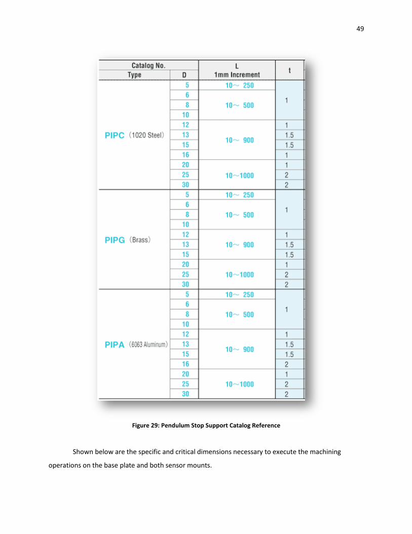
49
Figure 29: Pendulum Stop Support Catalog Reference
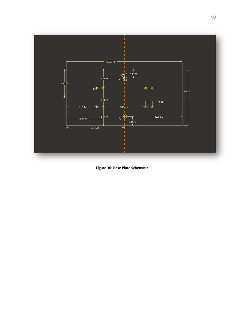
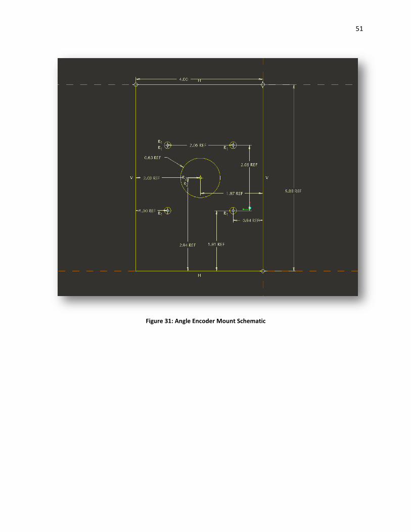
Shown below are the specific and critical dimensions necessary to execute the machining
operations on the base plate and both sensor mounts.
50
Figure 30: Base Plate Schematic
51
Figure 31: Angle Encoder Mount Schematic

52
Figure 32: Analog Angle Sensor Mount Schematic
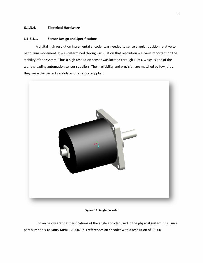
53
6.1.3.4. Electrical Hardware
6.1.3.4.1. Sensor Design and Specifications
A digital high resolution incremental encoder was needed to sense angular position relative to
pendulum movement. It was determined through simulation that resolution was very important on the
stability of the system. Thus a high resolution sensor was located through Turck, which is one of the
world’s leading automation sensor suppliers. Their reliability and precision are matched by few, thus
they were the perfect candidate for a sensor supplier.
Figure 33: Angle Encoder
Shown below are the specifications of the angle encoder used in the physical system. The Turck
part number is T8-5805-MP4T-36000. This references an encoder with a resolution of 36000
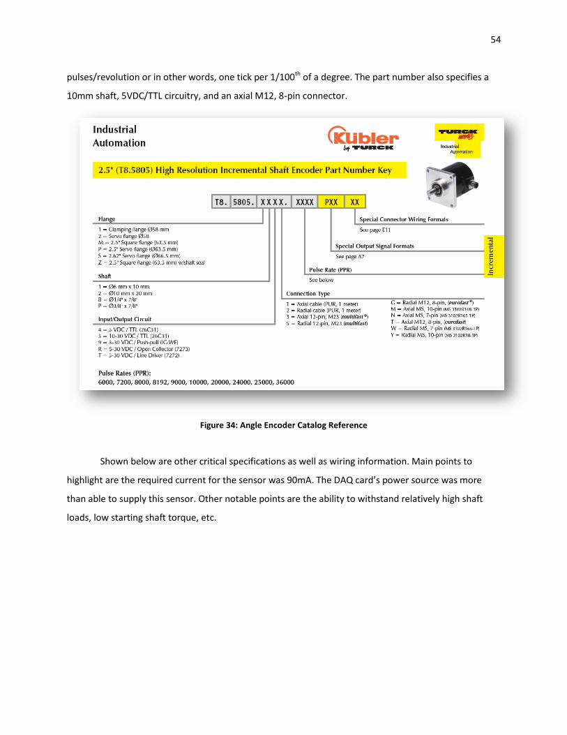
54
pulses/revolution or in other words, one tick per 1/100th of a degree. The part number also specifies a
10mm shaft, 5VDC/TTL circuitry, and an axial M12, 8-pin connector.
Figure 34: Angle Encoder Catalog Reference
Shown below are other critical specifications as well as wiring information. Main points to
highlight are the required current for the sensor was 90mA. The DAQ card’s power source was more
than able to supply this sensor. Other notable points are the ability to withstand relatively high shaft
loads, low starting shaft torque, etc.
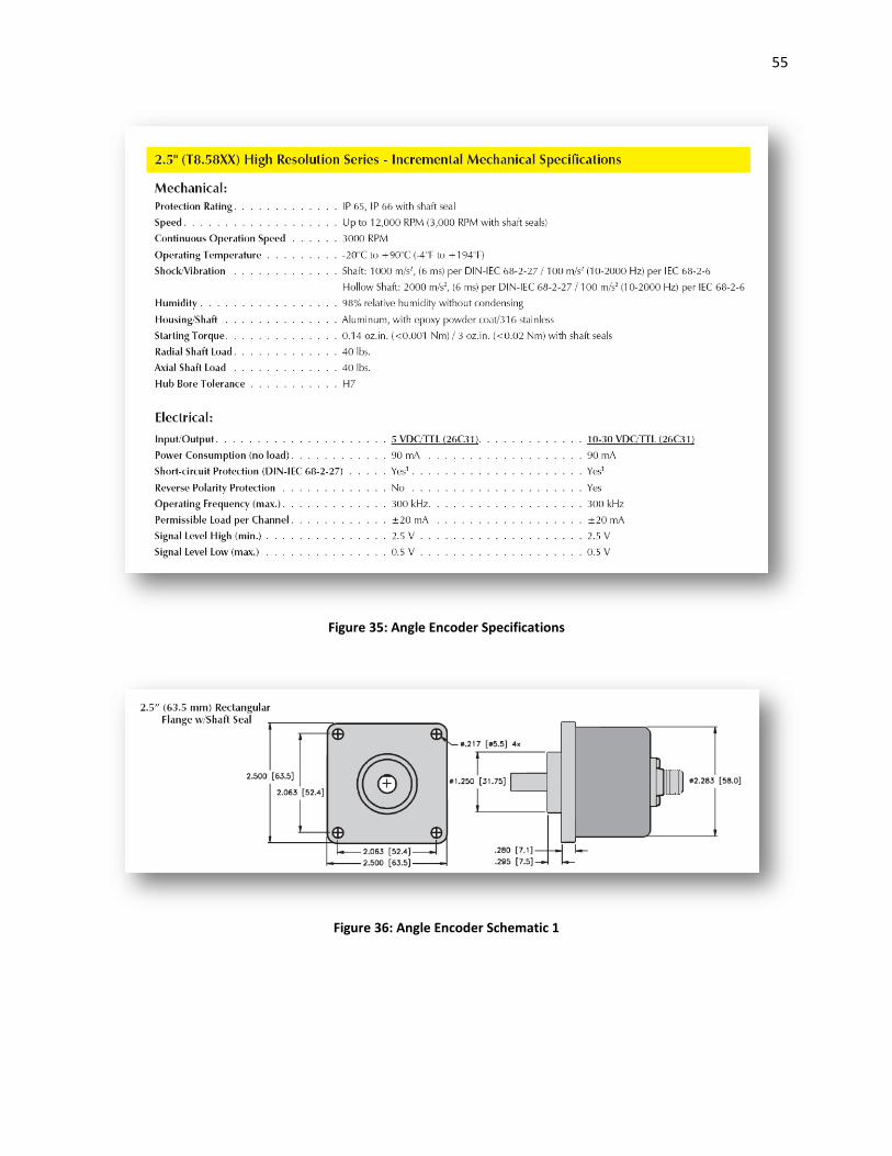
55
Figure 35: Angle Encoder Specifications
Figure 36: Angle Encoder Schematic 1
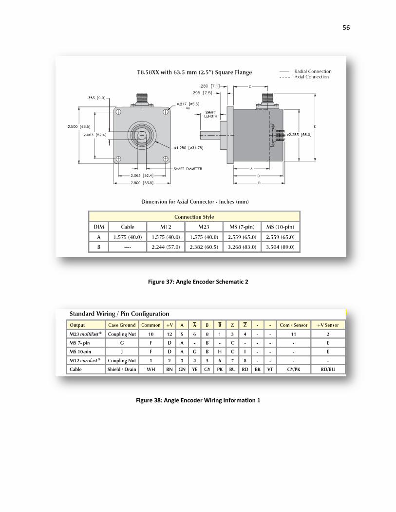
56
Figure 37: Angle Encoder Schematic 2
Figure 38: Angle Encoder Wiring Information 1
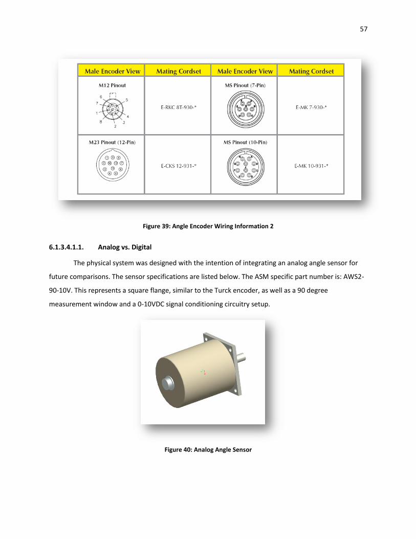
57
Figure 39: Angle Encoder Wiring Information 2
6.1.3.4.1.1. Analog vs. Digital
The physical system was designed with the intention of integrating an analog angle sensor for
future comparisons. The sensor specifications are listed below. The ASM specific part number is: AWS2-
90-10V. This represents a square flange, similar to the Turck encoder, as well as a 90 degree
measurement window and a 0-10VDC signal conditioning circuitry setup.
Figure 40: Analog Angle Sensor
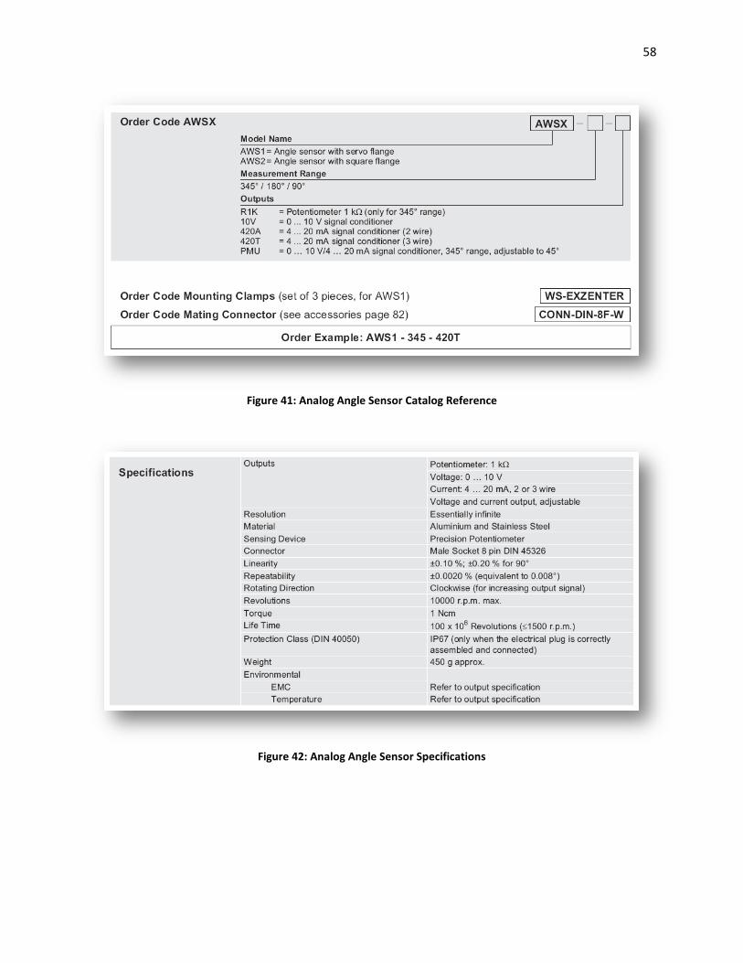
58
Figure 41: Analog Angle Sensor Catalog Reference
Figure 42: Analog Angle Sensor Specifications
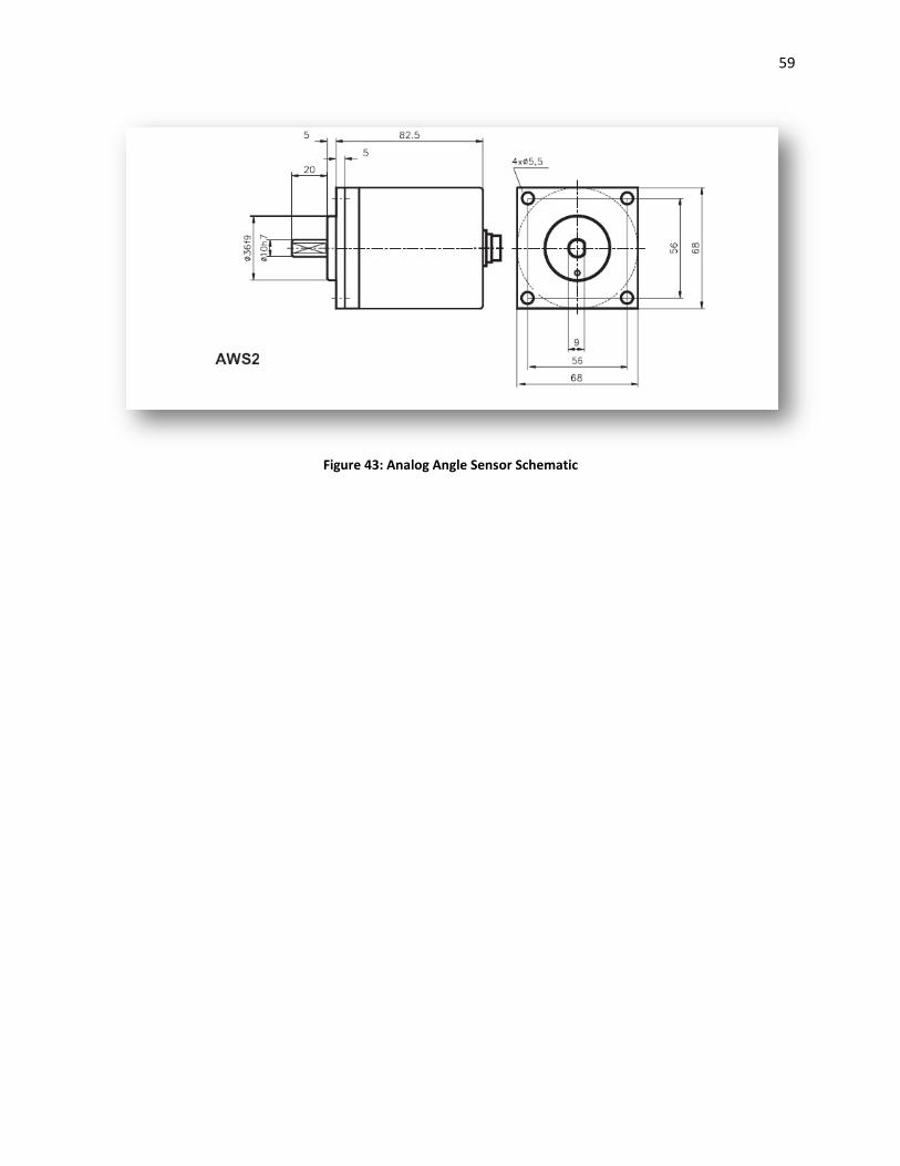
59
Figure 43: Analog Angle Sensor Schematic
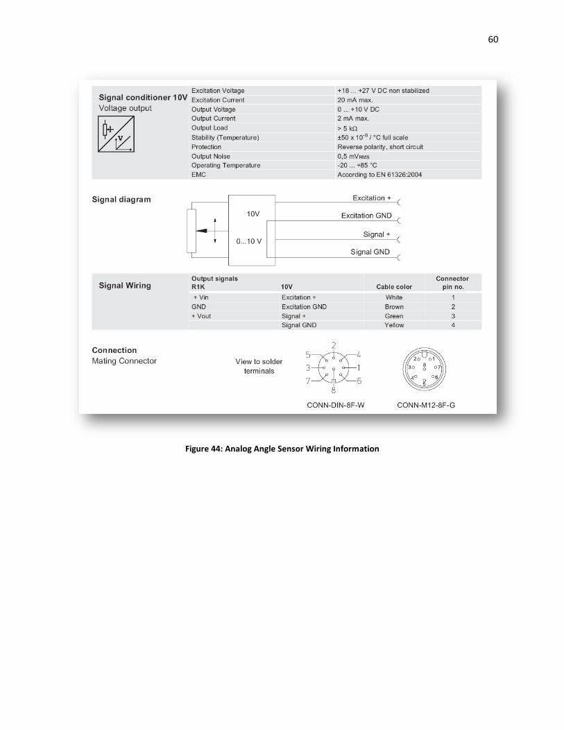
60
Figure 44: Analog Angle Sensor Wiring Information

61
6.1.3.4.2. DAQ Card Integration
Figure 45: NI PCI-6251 DAQ Card
The Turck angle encoder was linked to LabVIEW utilizing a M12 cable assembly and an NI-6251
Data Acquisition Card. This card was instrumental in the hand shaking between the sensor and the
computer. Additionally, this card served at the 5 volt power supply to the angular incremental encoder
sensor. Its specifications are listed below.
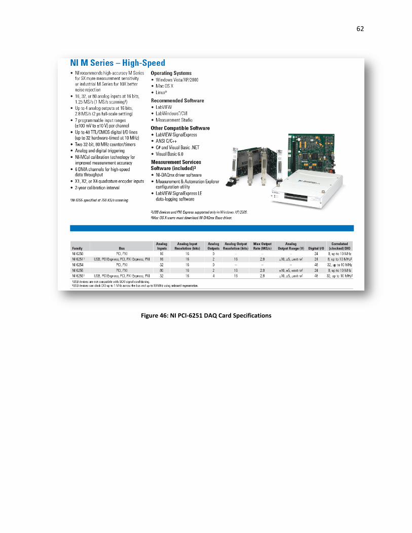
62
Figure 46: NI PCI-6251 DAQ Card Specifications
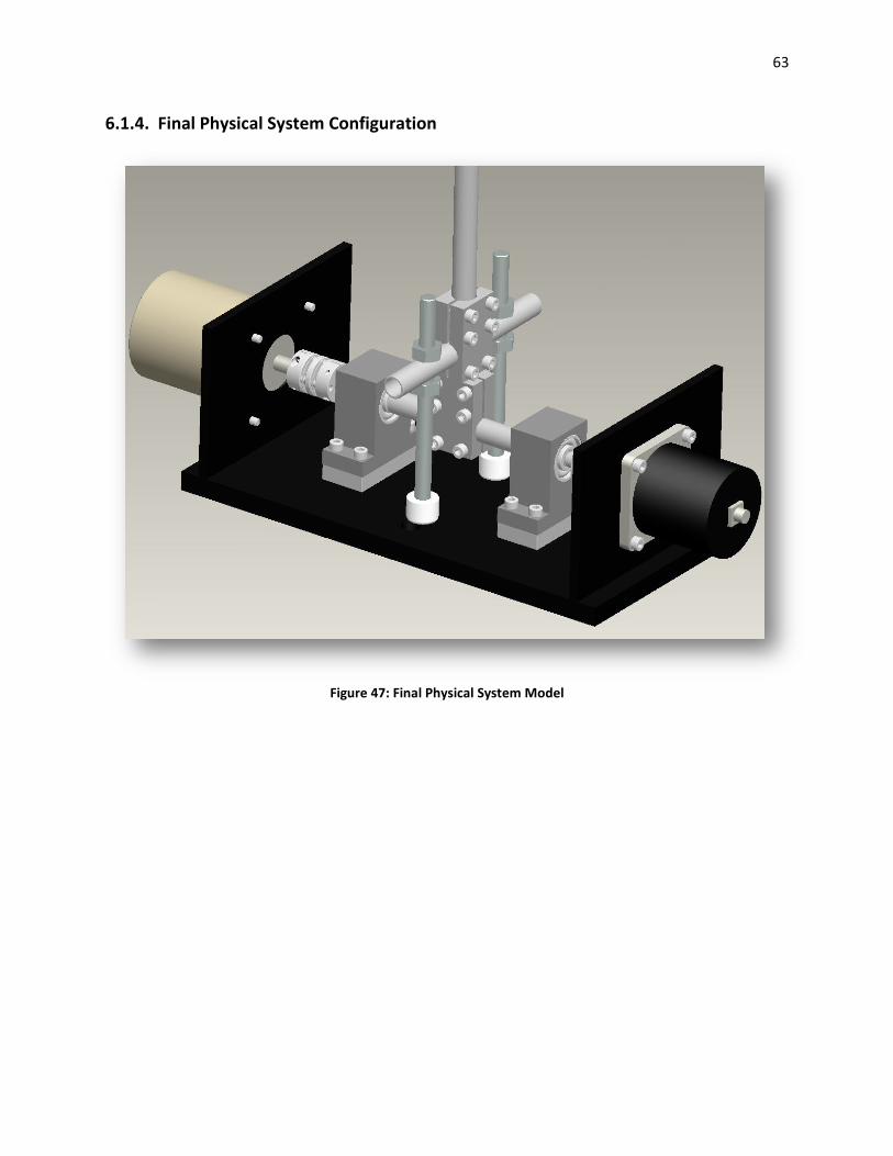
63
6.1.4. Final Physical System Configuration
Figure 47: Final Physical System Model
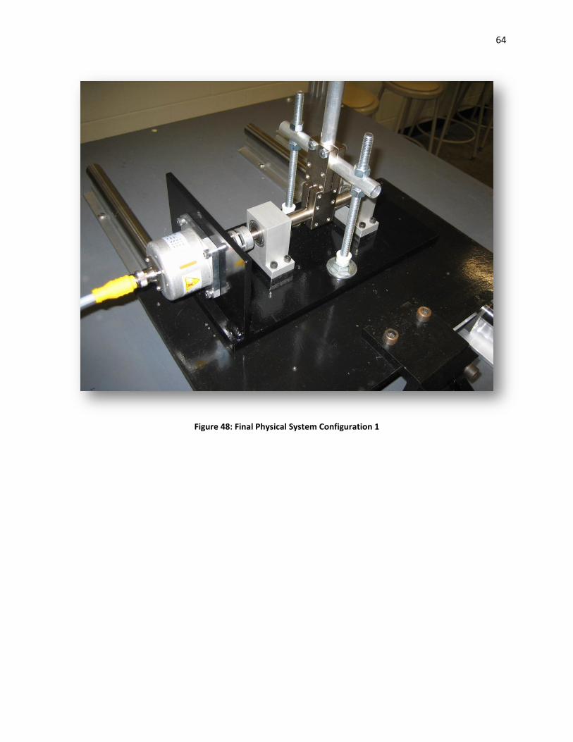
64
Figure 48: Final Physical System Configuration 1
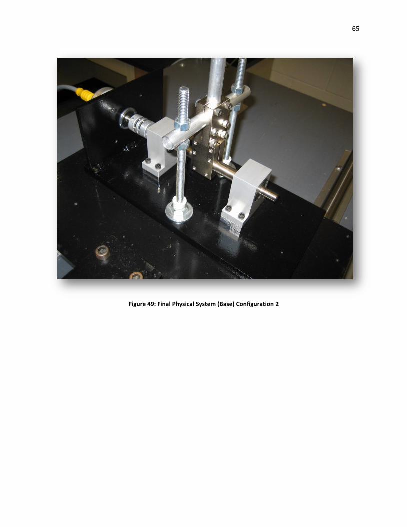
65
Figure 49: Final Physical System (Base) Configuration 2
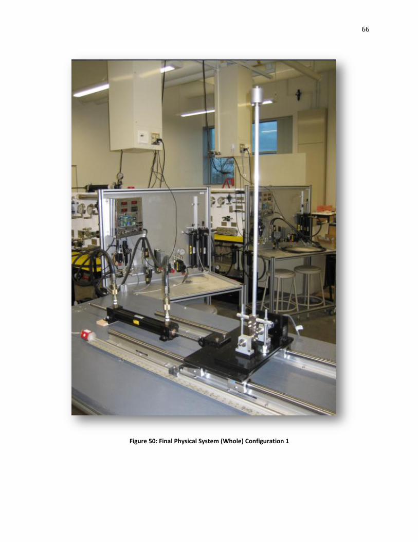
66
Figure 50: Final Physical System (Whole) Configuration 1

67
6.2. Software and Control Design
6.2.1. MATLAB and Software Tools
6.2.1.1. Introduction
As the systems engineers design become larger and more complex, certain processes need to be
defined in order to organize the project, provide consistency, and improve efficiency hindered by
performing the same functions repeatedly. Furthermore, documentation of the work needs to be
integrated throughout the project to allow developers, both currently working on the project and those
to work on the project afterwards, to readily understand the components being used. The inverted
pendulum system is a relatively simple system, requiring few sets of variables and component models.
However, in the interest of practicing concepts applicable to more realistic settings in the industry, a
process and set of software tools were developed to provide consistency, documentation, and efficiency
as the product was developed. The tools required time and effort at the beginning. However, once they
are made, the functions are defined for use as often as required, avoiding redundancy in work.
6.2.1.2. Overall Process
The process for creating a model in the inverted pendulum project begins with calibration files.
The quantitative component of the model is defined with these files. They are text files that define the
variables to be used in the model, ranging from physical dimensions to controller coefficients. As
progress is made in developing models, often a set of variables defining a system may have been
created that yields results worth documenting. However, as the project continues, changes to these
variables must be made. In this case, various calibration files can be made for the same model. Before
the Simulink model is opened, a graphical user interface (GUI) was created to allow a user to quickly
choose which calibration file to use in the model.
Once the variables have been defined, a Simulink block diagram model is used to qualitatively
define the dynamics of the real system. Transfer functions relating dynamic inputs to dynamic outputs
were used to define components within the system. Within the blocks or components of the system,
variables were used. These variables were defined in the model’s own workspace. Simulink’s model
explorer can be used to explore the variables in use in the model, which were originally defined in the
calibration file. Additionally, the majority of these variables were defined as objects, instead of simply
numbers. These objects allowed additional information, beyond the value of the variable, to be stored
68
with the variable, such as the units of the variable, the minimum and maximum allowable values, and a
description. This way, if a simulation of a model can be run, the user has access to the documentation of
the model within the model.
Once a simulation is run, a set of functions were called in the model’s callbacks to automatically
display certain information. First, a function is used to graph six essential signals: the pendulum angle,
the pendulum velocity, the sled position, the sled velocity, the valve spool input command, and the
valve spool position. These curves were plotted against the maximum and minimum allowed values for
successful performance. These plots were to give the user a quick over-all picture of the model’s
success. Next, a function would run through the numbers for each of those signals and print to the
command window “PASS” or “FAIL” test results for each signal, based on the signals maximum and
minimum values relative to performance criteria. This compliments the graphs by providing quantitative
test data. Finally, a graphical user interface is displayed that allows the user to view an animation based
on the resulting data. The animation speed can be adjusted, as well as the characteristics of the movie,
such as frames captured per second. This way, the validity of the data can be assessed, to some degree,
by how natural the pendulum motion is presented. Also, the animations can provide a sense of the
results better than simple graphs and numbers. Moreover, if the simulation yields a success, the time
histories of any of the signals in the model, beyond the six mentioned above, can be viewed through
scopes within the model. Before the user can decide the model is working properly and the simulation
yielded success in terms of performance, the user must check all of the signals within the model to verify
consistency and physical plausibility.
The chart shown in Figure 51 summarizes the overall process of development used in the project
that may be implemented similarly in other projects. The discussion is broken into three main sections,
the calibration files created to quantitatively define the system, the model itself created to qualitatively
define the system, and the resulting data produced from the model. The underlined text in the figure
represents functions. Refer to the appropriate sections in the report for a discussion of each function.
Also, Appendix… contains the code developed for each function. Now that these functions have been
created, development of the project simply means using the “makeCalinLikeness” function to create a
new calibration file, using the “checkParameters” function to verify consistency in the calibration file,
make a new model (with the appropriate callback function code discussed in section 6.2.1.5.3 Model
Tools) or modify the current model, and view the results of the modifications of the model. These
functions may later be improved on to automatically create a folder containing the numerical results,
graphical results, animation results, and parameters used to define the model. However, the current
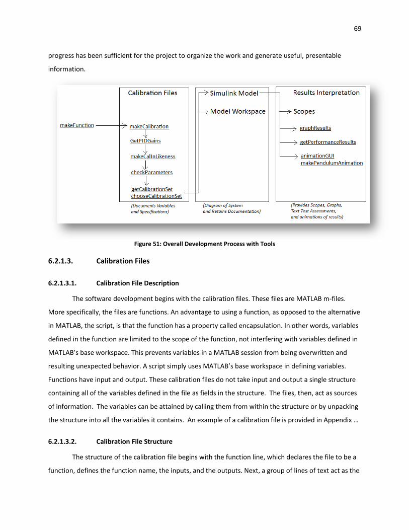
69
progress has been sufficient for the project to organize the work and generate useful, presentable
information.
Figure 51: Overall Development Process with Tools
6.2.1.3. Calibration Files
6.2.1.3.1. Calibration File Description
The software development begins with the calibration files. These files are MATLAB m-files.
More specifically, the files are functions. An advantage to using a function, as opposed to the alternative
in MATLAB, the script, is that the function has a property called encapsulation. In other words, variables
defined in the function are limited to the scope of the function, not interfering with variables defined in
MATLAB’s base workspace. This prevents variables in a MATLAB session from being overwritten and
resulting unexpected behavior. A script simply uses MATLAB’s base workspace in defining variables.
Functions have input and output. These calibration files do not take input and output a single structure
containing all of the variables defined in the file as fields in the structure. The files, then, act as sources
of information. The variables can be attained by calling them from within the structure or by unpacking
the structure into all the variables it contains. An example of a calibration file is provided in Appendix …
6.2.1.3.2. Calibration File Structure
The structure of the calibration file begins with the function line, which declares the file to be a
function, defines the function name, the inputs, and the outputs. Next, a group of lines of text act as the
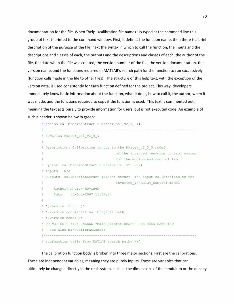
70
documentation for the file. When “help <calibration file name>” is typed at the command line this
group of text is printed to the command window. First, it defines the function name, then there is a brief
description of the purpose of the file, next the syntax in which to call the function, the inputs and the
descriptions and classes of each, the outputs and the descriptions and classes of each, the author of the
file, the date when the file was created, the version number of the file, the version documentation, the
version name, and the functions required in MATLAB’s search path for the function to run successively
(function calls made in the file to other files). The structure of this help text, with the exception of the
version data, is used consistently for each function defined for the project. This way, developers
immediately know basic information about the function, what it does, how to call it, the author, when it
was made, and the functions required to copy if the function is used. This text is commented out,
meaning the text acts purely to provide information for users, but is not executed code. An example of
such a header is shown below in green:
function calibrationStruct = Master_cal_v2_0_0()
%--------------------------------------------------------------------------
% FUNCTION Master_cal_v2_0_0
%
% Description: Calibration inputs to the Master_v2_0_0 model
% of the inverted pendulum control system
% for the motion and control lab.
% Syntax: calibrationStruct = Master_cal_v2_0_0()
% Inputs: N/A
% Outputs: calibrationStruct (class: struct) The input calibrations to the
% inverted_pendulum_control model
% Author: Andrew Hovingh
% Date: 15-Oct-2007 11:07:34
%
% !$version: 2_0_0 $!
% !$version documentation: Original set$!
% !$version name: $!
% DO NOT EDIT FILE UNLESS "makeCalibrationSet" HAS BEEN EXECUTED
% See also makeCalibrationSet
%--------------------------------------------------------------------------
% subfunction calls from MATLAB search path: N/A
The calibration function body is broken into three major sections. First are the calibrations.
These are independent variables, meaning they are purely inputs. These are variables that can
ultimately be changed directly in the real system, such as the dimensions of the pendulum or the density
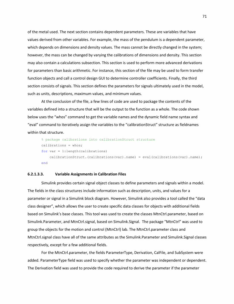
71
of the metal used. The next section contains dependent parameters. These are variables that have
values derived from other variables. For example, the mass of the pendulum is a dependent parameter,
which depends on dimensions and density values. The mass cannot be directly changed in the system;
however, the mass can be changed by varying the calibrations of dimensions and density. This section
may also contain a calculations subsection. This section is used to perform more advanced derivations
for parameters than basic arithmetic. For instance, this section of the file may be used to form transfer
function objects and call a control design GUI to determine controller coefficients. Finally, the third
section consists of signals. This section defines the parameters for signals ultimately used in the model,
such as units, descriptions, maximum values, and minimum values.
At the conclusion of the file, a few lines of code are used to package the contents of the
variables defined into a structure that will be the output to the function as a whole. The code shown
below uses the “whos” command to get the variable names and the dynamic field name syntax and
“eval” command to iteratively assign the variables to the “calibrationStruct” structure as fieldnames
within that structure.
% package calibrations into calibrationStruct structure
calibrations = whos;
for var = 1:length(calibrations)
calibrationStruct.(calibrations(var).name) = eval(calibrations(var).name);
end
6.2.1.3.3. Variable Assignments in Calibration Files
Simulink provides certain signal object classes to define parameters and signals within a model.
The fields in the class structures include information such as description, units, and values for a
parameter or signal in a Simulink block diagram. However, Simulink also provides a tool called the “data
class designer”, which allows the user to create specific data classes for objects with additional fields
based on Simulink’s base classes. This tool was used to create the classes MtnCtrl.parameter, based on
Simulink.Parameter, and MtnCtrl.signal, based on Simulink.Signal. The package “MtnCtrl” was used to
group the objects for the motion and control (MtnCtrl) lab. The MtnCtrl.parameter class and
MtnCtrl.signal class have all of the same attributes as the Simulink.Parameter and Simulink.Signal classes
respectively, except for a few additional fields.
For the MtnCtrl.parameter, the fields ParameterType, Derivation, CalFile, and SubSystem were
added. ParameterType field was used to specify whether the parameter was independent or dependent.
The Derivation field was used to provide the code required to derive the parameter if the parameter
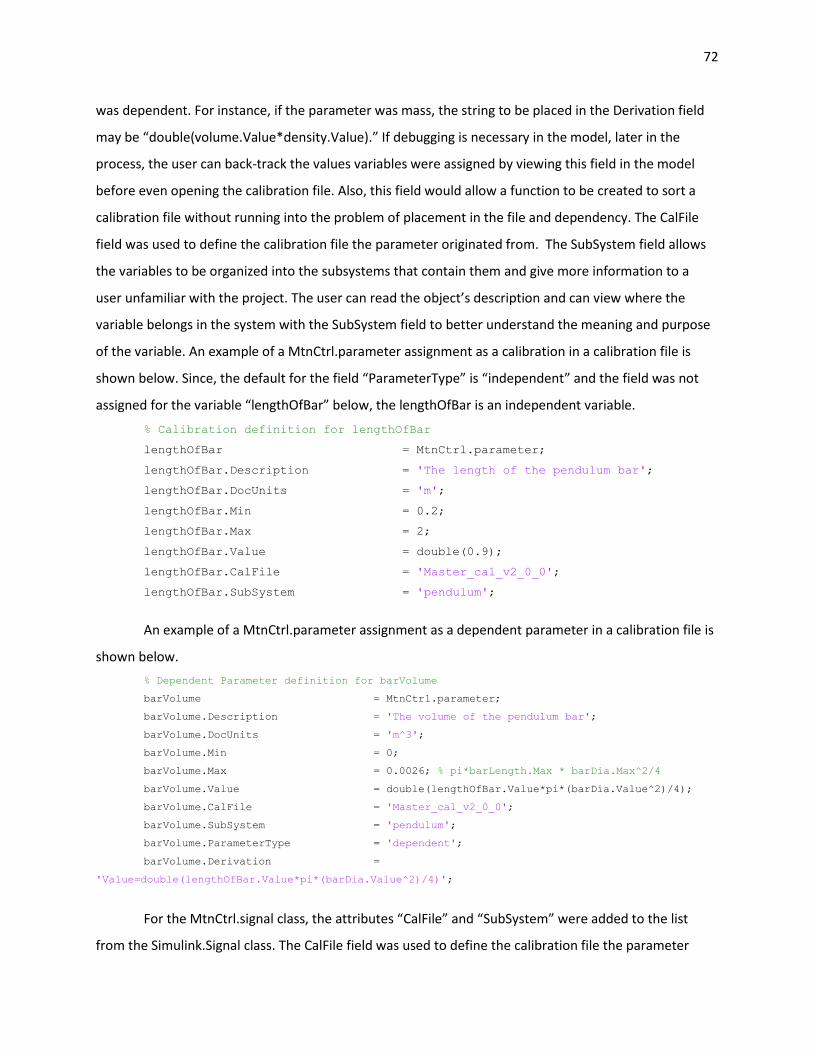
72
was dependent. For instance, if the parameter was mass, the string to be placed in the Derivation field
may be “double(volume.Value*density.Value).” If debugging is necessary in the model, later in the
process, the user can back-track the values variables were assigned by viewing this field in the model
before even opening the calibration file. Also, this field would allow a function to be created to sort a
calibration file without running into the problem of placement in the file and dependency. The CalFile
field was used to define the calibration file the parameter originated from. The SubSystem field allows
the variables to be organized into the subsystems that contain them and give more information to a
user unfamiliar with the project. The user can read the object’s description and can view where the
variable belongs in the system with the SubSystem field to better understand the meaning and purpose
of the variable. An example of a MtnCtrl.parameter assignment as a calibration in a calibration file is
shown below. Since, the default for the field “ParameterType” is “independent” and the field was not
assigned for the variable “lengthOfBar” below, the lengthOfBar is an independent variable.
% Calibration definition for lengthOfBar
lengthOfBar = MtnCtrl.parameter;
lengthOfBar.Description = 'The length of the pendulum bar';
lengthOfBar.DocUnits = 'm';
lengthOfBar.Min = 0.2;
lengthOfBar.Max = 2;
lengthOfBar.Value = double(0.9);
lengthOfBar.CalFile = 'Master_cal_v2_0_0';
lengthOfBar.SubSystem = 'pendulum';
An example of a MtnCtrl.parameter assignment as a dependent parameter in a calibration file is
shown below.
% Dependent Parameter definition for barVolume
barVolume = MtnCtrl.parameter;
barVolume.Description = 'The volume of the pendulum bar';
barVolume.DocUnits = 'm^3';
barVolume.Min = 0;
barVolume.Max = 0.0026; % pi*barLength.Max * barDia.Max^2/4
barVolume.Value = double(lengthOfBar.Value*pi*(barDia.Value^2)/4);
barVolume.CalFile = 'Master_cal_v2_0_0';
barVolume.SubSystem = 'pendulum';
barVolume.ParameterType = 'dependent';
barVolume.Derivation =
'Value=double(lengthOfBar.Value*pi*(barDia.Value^2)/4)';
For the MtnCtrl.signal class, the attributes “CalFile” and “SubSystem” were added to the list
from the Simulink.Signal class. The CalFile field was used to define the calibration file the parameter
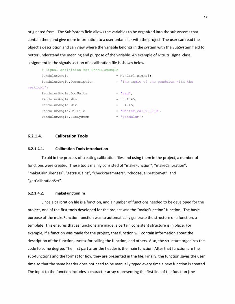
73
originated from. The SubSystem field allows the variables to be organized into the subsystems that
contain them and give more information to a user unfamiliar with the project. The user can read the
object’s description and can view where the variable belongs in the system with the SubSystem field to
better understand the meaning and purpose of the variable. An example of MtrCtrl.signal class
assignment in the signals section of a calibration file is shown below.
% Signal definition for PendulumAngle
PendulumAngle = MtnCtrl.signal;
PendulumAngle.Description = 'The angle of the pendulum with the
vertical';
PendulumAngle.DocUnits = 'rad';
PendulumAngle.Min = -0.1745;
PendulumAngle.Max = 0.1745;
PendulumAngle.CalFile = 'Master_cal_v2_0_0';
PendulumAngle.SubSystem = 'pendulum';
6.2.1.4. Calibration Tools
6.2.1.4.1. Calibration Tools Introduction
To aid in the process of creating calibration files and using them in the project, a number of
functions were created. These tools mainly consisted of “makeFunction”, “makeCalibration”,
”makeCalInLikeness”, “getPIDGains”, “checkParameters”, “chooseCalibrationSet”, and
“getCalibrationSet”.
6.2.1.4.2. makeFunction.m
Since a calibration file is a function, and a number of functions needed to be developed for the
project, one of the first tools developed for the project was the “makeFunction” function. The basic
purpose of the makeFunction function was to automatically generate the structure of a function, a
template. This ensures that as functions are made, a certain consistent structure is in place. For
example, if a function was made for the project, that function will contain information about the
description of the function, syntax for calling the function, and others. Also, the structure organizes the
code to some degree. The first part after the header is the main function. After that function are the
sub-functions and the format for how they are presented in the file. Finally, the function saves the user
time so that the same header does not need to be manually typed every time a new function is created.
The input to the function includes a character array representing the first line of the function (the
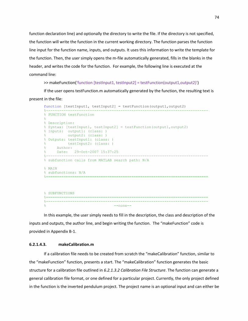
74
function declaration line) and optionally the directory to write the file. If the directory is not specified,
the function will write the function in the current working directory. The function parses the function
line input for the function name, inputs, and outputs. It uses this information to write the template for
the function. Then, the user simply opens the m-file automatically generated, fills in the blanks in the
header, and writes the code for the function. For example, the following line is executed at the
command line:
>> makeFunction('function [testInput1, testInput2] = testFunction(output1,output2)')
If the user opens testFunction.m automatically generated by the function, the resulting text is
present in the file:
function [testInput1, testInput2] = testFunction(output1,output2)
%--------------------------------------------------------------------------
% FUNCTION testFunction
%
% Description:
% Syntax: [testInput1, testInput2] = testFunction(output1,output2)
% Inputs: output1: (class: )
% output2: (class: )
% Outputs: testInput1: (class: )
% testInput2: (class: )
% Author:
% Date: 29-Oct-2007 15:37:25
%--------------------------------------------------------------------------
% subfunction calls from MATLAB search path: N/A
% MAIN
% subfunctions: N/A
%==========================================================================
% SUBFUNCTIONS
%==========================================================================
%--------------------------------------------------------------------------
% --none--
In this example, the user simply needs to fill in the description, the class and description of the
inputs and outputs, the author line, and begin writing the function. The “makeFunction” code is
provided in Appendix B-1.
6.2.1.4.3. makeCalibration.m
If a calibration file needs to be created from scratch the “makeCalibration” function, similar to
the “makeFunction” function, presents a start. The “makeCalibration” function generates the basic
structure for a calibration file outlined in 6.2.1.3.2 Calibration File Structure. The function can generate a
general calibration file format, or one defined for a particular project. Currently, the only project defined
in the function is the inverted pendulum project. The project name is an optional input and can either be
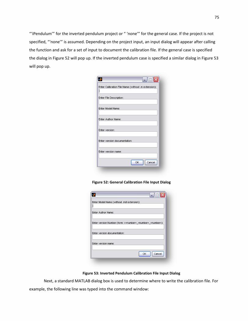
75
“‘iPendulum’” for the inverted pendulum project or “ ‘none’” for the general case. If the project is not
specified, “‘none’” is assumed. Depending on the project input, an input dialog will appear after calling
the function and ask for a set of input to document the calibration file. If the general case is specified
the dialog in Figure 52 will pop up. If the inverted pendulum case is specified a similar dialog in Figure 53
will pop up.
Figure 52: General Calibration File Input Dialog
Figure 53: Inverted Pendulum Calibration File Input Dialog
Next, a standard MATLAB dialog box is used to determine where to write the calibration file. For
example, the following line was typed into the command window:
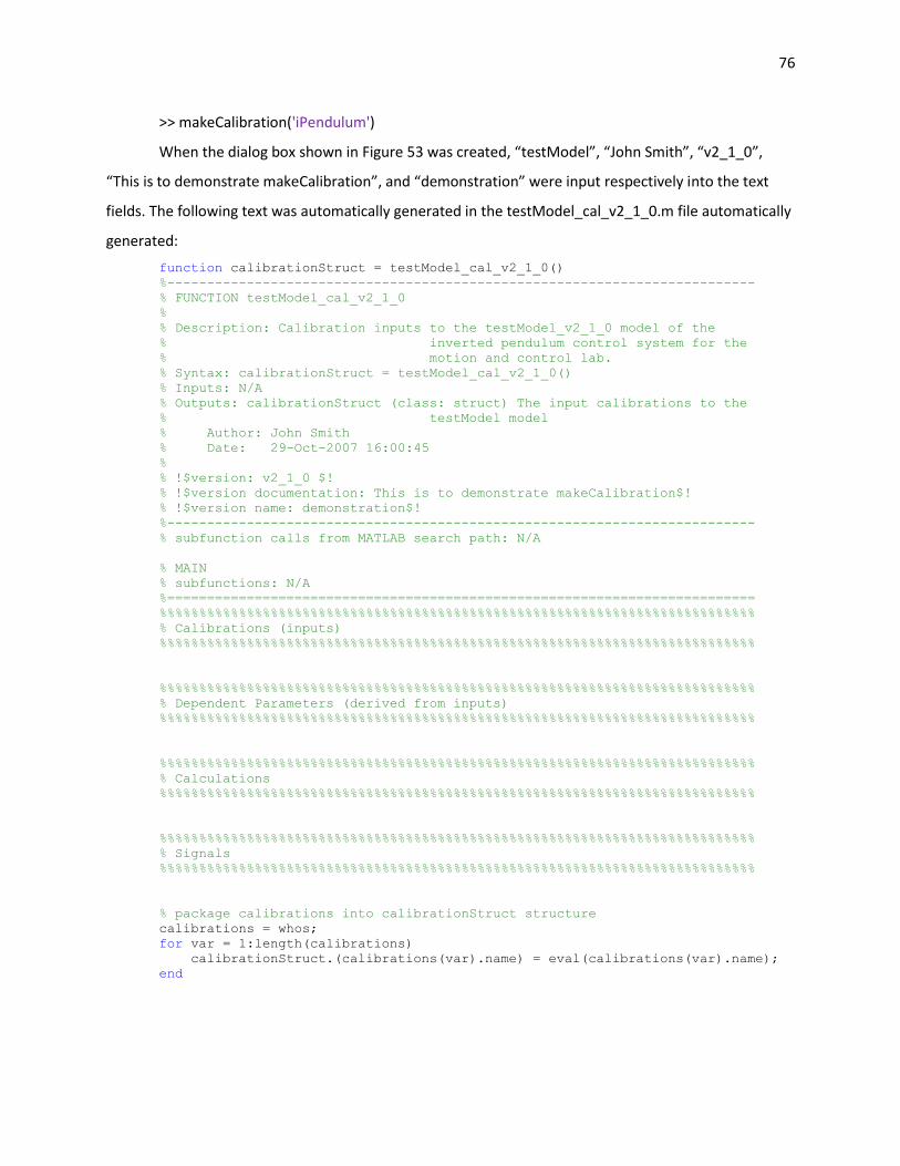
76
>> makeCalibration('iPendulum')
When the dialog box shown in Figure 53 was created, “testModel”, “John Smith”, “v2_1_0”,
“This is to demonstrate makeCalibration”, and “demonstration” were input respectively into the text
fields. The following text was automatically generated in the testModel_cal_v2_1_0.m file automatically
generated:
function calibrationStruct = testModel_cal_v2_1_0()
%--------------------------------------------------------------------------
% FUNCTION testModel_cal_v2_1_0
%
% Description: Calibration inputs to the testModel_v2_1_0 model of the
% inverted pendulum control system for the
% motion and control lab.
% Syntax: calibrationStruct = testModel_cal_v2_1_0()
% Inputs: N/A
% Outputs: calibrationStruct (class: struct) The input calibrations to the
% testModel model
% Author: John Smith
% Date: 29-Oct-2007 16:00:45
%
% !$version: v2_1_0 $!
% !$version documentation: This is to demonstrate makeCalibration$!
% !$version name: demonstration$!
%--------------------------------------------------------------------------
% subfunction calls from MATLAB search path: N/A
% MAIN
% subfunctions: N/A
%==========================================================================
%%%%%%%%%%%%%%%%%%%%%%%%%%%%%%%%%%%%%%%%%%%%%%%%%%%%%%%%%%%%%%%%%%%%%%%%%%%
% Calibrations (inputs)
%%%%%%%%%%%%%%%%%%%%%%%%%%%%%%%%%%%%%%%%%%%%%%%%%%%%%%%%%%%%%%%%%%%%%%%%%%%
%%%%%%%%%%%%%%%%%%%%%%%%%%%%%%%%%%%%%%%%%%%%%%%%%%%%%%%%%%%%%%%%%%%%%%%%%%%
% Dependent Parameters (derived from inputs)
%%%%%%%%%%%%%%%%%%%%%%%%%%%%%%%%%%%%%%%%%%%%%%%%%%%%%%%%%%%%%%%%%%%%%%%%%%%
%%%%%%%%%%%%%%%%%%%%%%%%%%%%%%%%%%%%%%%%%%%%%%%%%%%%%%%%%%%%%%%%%%%%%%%%%%%
% Calculations
%%%%%%%%%%%%%%%%%%%%%%%%%%%%%%%%%%%%%%%%%%%%%%%%%%%%%%%%%%%%%%%%%%%%%%%%%%%
%%%%%%%%%%%%%%%%%%%%%%%%%%%%%%%%%%%%%%%%%%%%%%%%%%%%%%%%%%%%%%%%%%%%%%%%%%%
% Signals
%%%%%%%%%%%%%%%%%%%%%%%%%%%%%%%%%%%%%%%%%%%%%%%%%%%%%%%%%%%%%%%%%%%%%%%%%%%
% package calibrations into calibrationStruct structure
calibrations = whos;
for var = 1:length(calibrations)
calibrationStruct.(calibrations(var).name) = eval(calibrations(var).name);
end
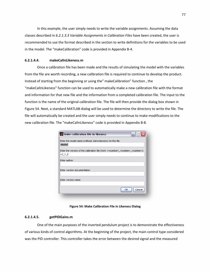
77
In this example, the user simply needs to write the variable assignments. Assuming the data
classes described in 6.2.1.3.3 Variable Assignments in Calibration Files have been created, the user is
recommended to use the format described in the section to write definitions for the variables to be used
in the model. The “makeCalibration” code is provided in Appendix B-4.
6.2.1.4.4. makeCalInLikeness.m
Once a calibration file has been made and the results of simulating the model with the variables
from the file are worth recording, a new calibration file is required to continue to develop the product.
Instead of starting from the beginning or using the” makeCalibration” function , the
“makeCalInLikeness” function can be used to automatically make a new calibration file with the format
and information for that new file and the information from a completed calibration file. The input to the
function is the name of the original calibration file. The file will then provide the dialog box shown in
Figure 54. Next, a standard MATLAB dialog will be used to determine the directory to write the file. The
file will automatically be created and the user simply needs to continue to make modifications to the
new calibration file. The “makeCalInLikeness” code is provided in Appendix B-8.
Figure 54: Make Calibration File in Likeness Dialog
6.2.1.4.5. getPIDGains.m
One of the main purposes of the inverted pendulum project is to demonstrate the effectiveness
of various kinds of control algorithms. At the beginning of the project, the main control type considered
was the PID controller. This controller takes the error between the desired signal and the measured
78
signal and performs three operations on it. It multiplies it by a proportional gain, integrates it and
multiplies that by an integral gain, and takes the derivative of it and multiplies it by a derivative gain.
The result of these operations are added together to become the command to the system’s actuator.
Any of these gains can be set to zero to reduce the controller to a different combination, such as a PI,
proportional derivative, controller. This function can be useful for quickly changing the gains and using a
Root locus approach to assigning them. Currently, the function simply assigns the appropriate gains
based on the gain selection on the root locus diagram by the user. However, the function may be
expanded in the future to automatically display the step response of the system for example. This was
not done in the inverted pendulum project because the system is unstable. The step response is not
necessarily a meaningful result for the system. The meaningful result, in this case, is the result of the
Simulink model. Therefore, the user could select gains when the model is initialized, view the results,
and reinitialize the workspace, where the “getPIDGains” function is called in the calibration file used, to
assign new coefficients with the root locus diagram. This process can quickly be repeated to see the
changes to the system by selecting different gains in the root locus diagram.
The function takes only two inputs and outputs a single component. The first input to the
function is a transfer function object that represents the open loop transfer function of the
uncompensated system. Refer to MATLAB’s help documentation for transfer functions in MATLAB. The
second input is an array of double type indicating the initial gains to test. The entries in the array are the
proportional, derivative, and integral gains respectively. The output of the function is an array of double
type indicating the gains the user selected. The entries, as in the input array, are the proportional,
derivative, and integral gains respectively.
As shown in Figure 55, the figure provides the user with a number of options for tuning the
controller gains. At the top of the window exists three text boxes. These boxes display the current gain
selected. When the “Reset” button below each box is green, the number in the text box represents the
initial gain passed to the function. If the button below the box is yellow, this indicates the value in the
box is acceptable (it is a number), but the value is different than the initial input value. If the value in the
text box is not valid, the “Reset” button below the box will be red and a warning will be printed to the
command window. The “Reset” button below each box can be pressed at any time to reset the value in
the text box to the original value. The number in each text box can be changed by manually typing a
number in the box, pressing the “Reset” button to reset the value back to its original number, or by
using the root locus design option. Below the “Reset” buttons is a set of radio buttons labeled
“Proportional”, “Integral”, and “Derivative”. The button selected represents the gain to vary in the root
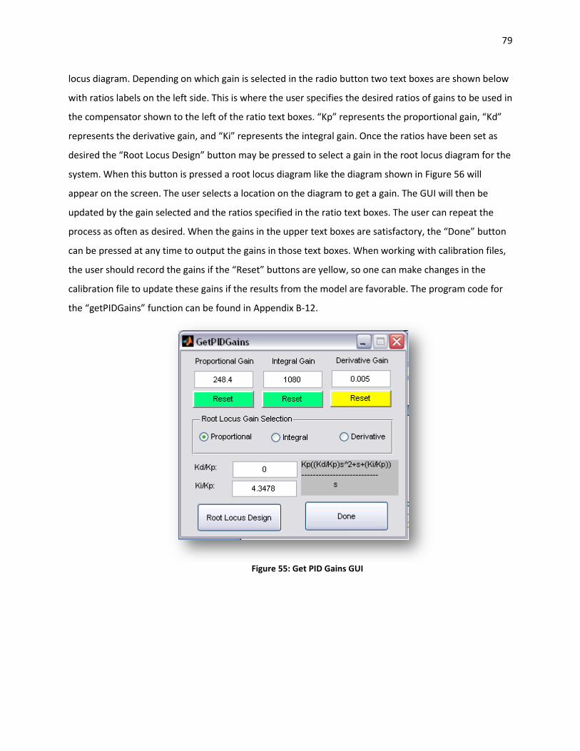
79
locus diagram. Depending on which gain is selected in the radio button two text boxes are shown below
with ratios labels on the left side. This is where the user specifies the desired ratios of gains to be used in
the compensator shown to the left of the ratio text boxes. “Kp” represents the proportional gain, “Kd”
represents the derivative gain, and “Ki” represents the integral gain. Once the ratios have been set as
desired the “Root Locus Design” button may be pressed to select a gain in the root locus diagram for the
system. When this button is pressed a root locus diagram like the diagram shown in Figure 56 will
appear on the screen. The user selects a location on the diagram to get a gain. The GUI will then be
updated by the gain selected and the ratios specified in the ratio text boxes. The user can repeat the
process as often as desired. When the gains in the upper text boxes are satisfactory, the “Done” button
can be pressed at any time to output the gains in those text boxes. When working with calibration files,
the user should record the gains if the “Reset” buttons are yellow, so one can make changes in the
calibration file to update these gains if the results from the model are favorable. The program code for
the “getPIDGains” function can be found in Appendix B-12.
Figure 55: Get PID Gains GUI
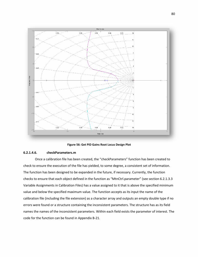
80
Figure 56: Get PID Gains Root Locus Design Plot
6.2.1.4.6. checkParameters.m
Once a calibration file has been created, the “checkParameters” function has been created to
check to ensure the execution of the file has yielded, to some degree, a consistent set of information.
The function has been designed to be expanded in the future, if necessary. Currently, the function
checks to ensure that each object defined in the function as “MtnCtrl.parameter” (see section 6.2.1.3.3
Variable Assignments in Calibration Files) has a value assigned to it that is above the specified minimum
value and below the specified maximum value. The function accepts as its input the name of the
calibration file (including the file extension) as a character array and outputs an empty double type if no
errors were found or a structure containing the inconsistent parameters. The structure has as its field
names the names of the inconsistent parameters. Within each field exists the parameter of interest. The
code for the function can be found in Appendix B-21.

81
6.2.1.4.7. chooseCalibrationSet.m
Once the calibration file or files have been created for a file, the files are used to populate the
model’s workspace. The purpose of the function “chooseCalibrationSet” is to provide an interface for
the user to select a calibration file from the list the function was provided. The function takes three
inputs: the model name, the model version, and a structure containing the calibration file names. The
model name and version are used to organize the list for ease of use. The structure contains fields
“calibrationSets” and “calibrationMats.” “calibrationMats” has not been used in the project and is
present to be possibly expanded on in the future. The “name” field is present within each calibration
field, and this is where the file names are stored. The function, then organizes the list of names within
this structure, and presents them in a list box on the graphical user interface (GUI) shown in Figure 57 .
To the right of the list box are three radio buttons. They are “View MAT Files”, “View Different
Versions”, and “View Other Model Calibration Sets”. The “View MAT Files” simply includes in the list the
.mat files that could be used as calibration files. This function has no real use in this particular project,
but may be used at a later date in development. If “View Different Versions” is not selected, only the file
versions corresponding to the model input data are listed. To view previous or later versions select
“View Different Versions.” Finally, to view calibration files for other models altogether select “View
Other Model Calibration Sets”. By default all of these options are not selected, only showing m-files
associated with the particular model of the specified version. Additionally, the GUI allows the user to
press “View Calibration Documentation”, which prompts a message box containing the text it reads
from the header of the calibration file indicating version documentation. Pressing “Selection Help” has
the effect of typing “help <selected calibration file name>” in the command line, printing the header of
the file in the command window. Once “Load Calibration Set” is pressed the selected file name is the
output of the function in the form of a character array. The chooseCalibrationSet code can be found in
Appendix B-22.
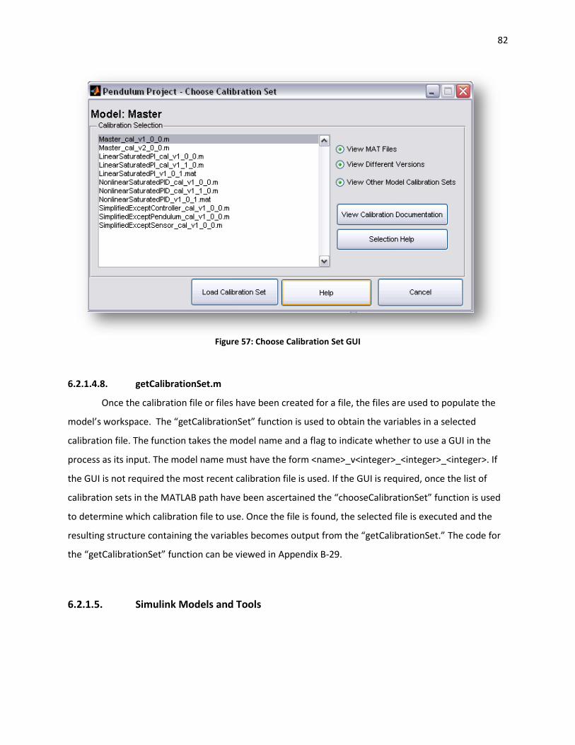
82
Figure 57: Choose Calibration Set GUI
6.2.1.4.8. getCalibrationSet.m
Once the calibration file or files have been created for a file, the files are used to populate the
model’s workspace. The “getCalibrationSet” function is used to obtain the variables in a selected
calibration file. The function takes the model name and a flag to indicate whether to use a GUI in the
process as its input. The model name must have the form <name>_v<integer>_<integer>_<integer>. If
the GUI is not required the most recent calibration file is used. If the GUI is required, once the list of
calibration sets in the MATLAB path have been ascertained the “chooseCalibrationSet” function is used
to determine which calibration file to use. Once the file is found, the selected file is executed and the
resulting structure containing the variables becomes output from the “getCalibrationSet.” The code for
the “getCalibrationSet” function can be viewed in Appendix B-29.
6.2.1.5. Simulink Models and Tools
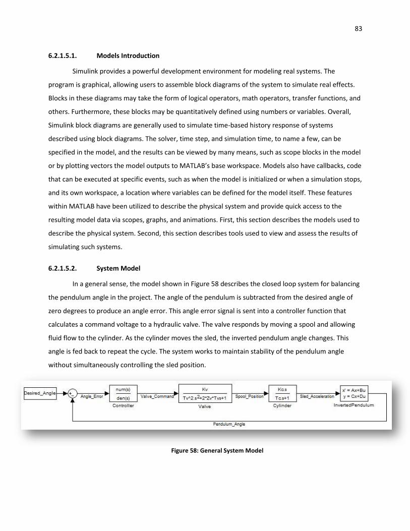
83
6.2.1.5.1. Models Introduction
Simulink provides a powerful development environment for modeling real systems. The
program is graphical, allowing users to assemble block diagrams of the system to simulate real effects.
Blocks in these diagrams may take the form of logical operators, math operators, transfer functions, and
others. Furthermore, these blocks may be quantitatively defined using numbers or variables. Overall,
Simulink block diagrams are generally used to simulate time-based history response of systems
described using block diagrams. The solver, time step, and simulation time, to name a few, can be
specified in the model, and the results can be viewed by many means, such as scope blocks in the model
or by plotting vectors the model outputs to MATLAB’s base workspace. Models also have callbacks, code
that can be executed at specific events, such as when the model is initialized or when a simulation stops,
and its own workspace, a location where variables can be defined for the model itself. These features
within MATLAB have been utilized to describe the physical system and provide quick access to the
resulting model data via scopes, graphs, and animations. First, this section describes the models used to
describe the physical system. Second, this section describes tools used to view and assess the results of
simulating such systems.
6.2.1.5.2. System Model
In a general sense, the model shown in Figure 58 describes the closed loop system for balancing
the pendulum angle in the project. The angle of the pendulum is subtracted from the desired angle of
zero degrees to produce an angle error. This angle error signal is sent into a controller function that
calculates a command voltage to a hydraulic valve. The valve responds by moving a spool and allowing
fluid flow to the cylinder. As the cylinder moves the sled, the inverted pendulum angle changes. This
angle is fed back to repeat the cycle. The system works to maintain stability of the pendulum angle
without simultaneously controlling the sled position.
Figure 58: General System Model
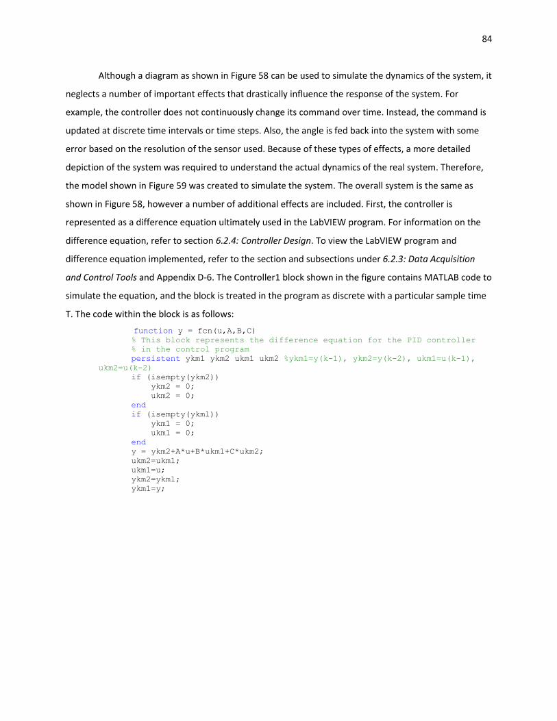
84
Although a diagram as shown in Figure 58 can be used to simulate the dynamics of the system, it
neglects a number of important effects that drastically influence the response of the system. For
example, the controller does not continuously change its command over time. Instead, the command is
updated at discrete time intervals or time steps. Also, the angle is fed back into the system with some
error based on the resolution of the sensor used. Because of these types of effects, a more detailed
depiction of the system was required to understand the actual dynamics of the real system. Therefore,
the model shown in Figure 59 was created to simulate the system. The overall system is the same as
shown in Figure 58, however a number of additional effects are included. First, the controller is
represented as a difference equation ultimately used in the LabVIEW program. For information on the
difference equation, refer to section 6.2.4: Controller Design. To view the LabVIEW program and
difference equation implemented, refer to the section and subsections under 6.2.3: Data Acquisition
and Control Tools and Appendix D-6. The Controller1 block shown in the figure contains MATLAB code to
simulate the equation, and the block is treated in the program as discrete with a particular sample time
T. The code within the block is as follows:
function y = fcn(u,A,B,C) % This block represents the difference equation for the PID controller
% in the control program
persistent ykm1 ykm2 ukm1 ukm2 %ykm1=y(k-1), ykm2=y(k-2), ukm1=u(k-1),
ukm2=u(k-2)
if (isempty(ykm2))
ykm2 = 0;
ukm2 = 0;
end
if (isempty(ykm1))
ykm1 = 0;
ukm1 = 0;
end
y = ykm2+A*u+B*ukm1+C*ukm2;
ukm2=ukm1;
ukm1=u;
ykm2=ykm1;
ykm1=y;
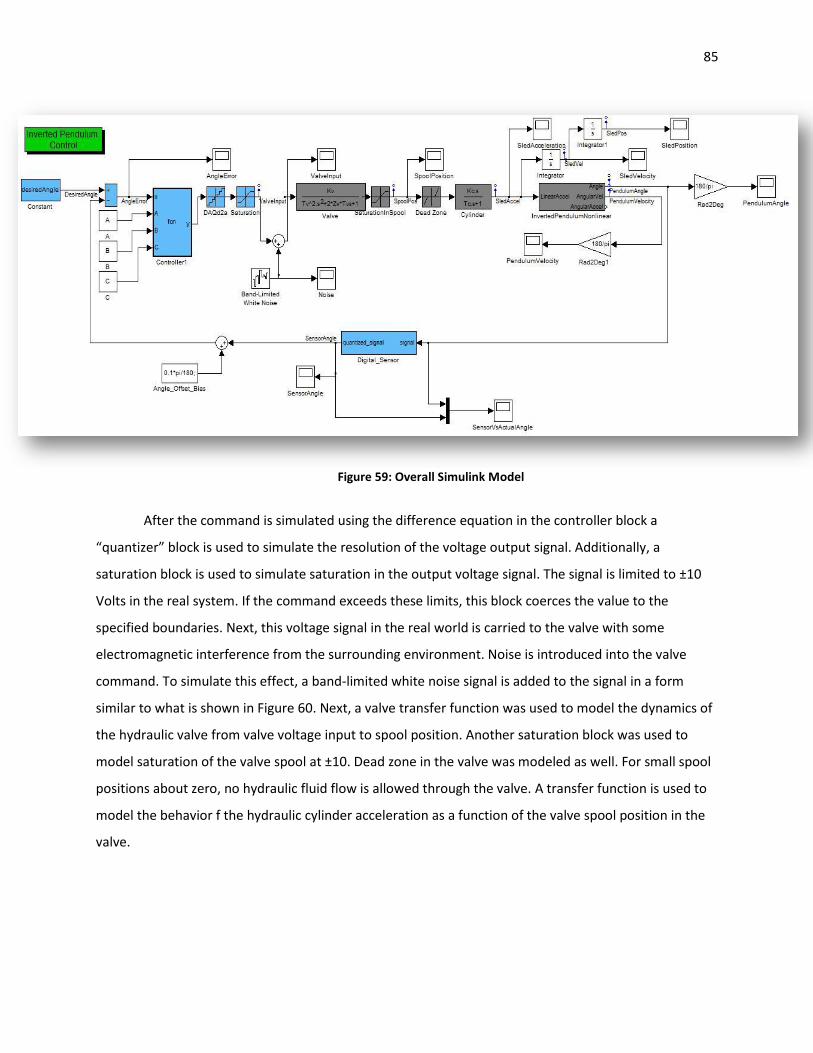
85
Figure 59: Overall Simulink Model
After the command is simulated using the difference equation in the controller block a
“quantizer” block is used to simulate the resolution of the voltage output signal. Additionally, a
saturation block is used to simulate saturation in the output voltage signal. The signal is limited to ±10
Volts in the real system. If the command exceeds these limits, this block coerces the value to the
specified boundaries. Next, this voltage signal in the real world is carried to the valve with some
electromagnetic interference from the surrounding environment. Noise is introduced into the valve
command. To simulate this effect, a band-limited white noise signal is added to the signal in a form
similar to what is shown in Figure 60. Next, a valve transfer function was used to model the dynamics of
the hydraulic valve from valve voltage input to spool position. Another saturation block was used to
model saturation of the valve spool at ±10. Dead zone in the valve was modeled as well. For small spool
positions about zero, no hydraulic fluid flow is allowed through the valve. A transfer function is used to
model the behavior f the hydraulic cylinder acceleration as a function of the valve spool position in the
valve.
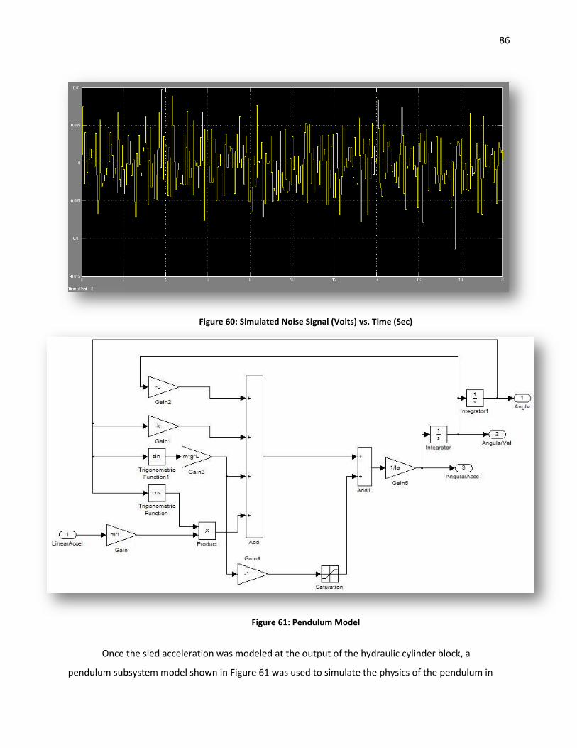
86
Figure 60: Simulated Noise Signal (Volts) vs. Time (Sec)
Figure 61: Pendulum Model
Once the sled acceleration was modeled at the output of the hydraulic cylinder block, a
pendulum subsystem model shown in Figure 61 was used to simulate the physics of the pendulum in
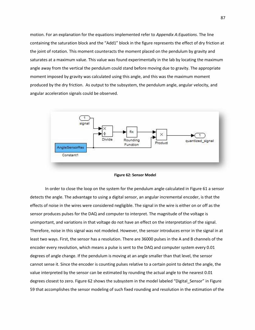
87
motion. For an explanation for the equations implemented refer to Appendix A:Equations. The line
containing the saturation block and the “Add1” block in the figure represents the effect of dry friction at
the joint of rotation. This moment counteracts the moment placed on the pendulum by gravity and
saturates at a maximum value. This value was found experimentally in the lab by locating the maximum
angle away from the vertical the pendulum could stand before moving due to gravity. The appropriate
moment imposed by gravity was calculated using this angle, and this was the maximum moment
produced by the dry friction. As output to the subsystem, the pendulum angle, angular velocity, and
angular acceleration signals could be observed.
Figure 62: Sensor Model
In order to close the loop on the system for the pendulum angle calculated in Figure 61 a sensor
detects the angle. The advantage to using a digital sensor, an angular incremental encoder, is that the
effects of noise in the wires were considered negligible. The signal in the wire is either on or off as the
sensor produces pulses for the DAQ and computer to interpret. The magnitude of the voltage is
unimportant, and variations in that voltage do not have an effect on the interpretation of the signal.
Therefore, noise in this signal was not modeled. However, the sensor introduces error in the signal in at
least two ways. First, the sensor has a resolution. There are 36000 pulses in the A and B channels of the
encoder every revolution, which means a pulse is sent to the DAQ and computer system every 0.01
degrees of angle change. If the pendulum is moving at an angle smaller than that level, the sensor
cannot sense it. Since the encoder is counting pulses relative to a certain point to detect the angle, the
value interpreted by the sensor can be estimated by rounding the actual angle to the nearest 0.01
degrees closest to zero. Figure 62 shows the subsystem in the model labeled “Digital_Sensor” in Figure
59 that accomplishes the sensor modeling of such fixed rounding and resolution in the estimation of the
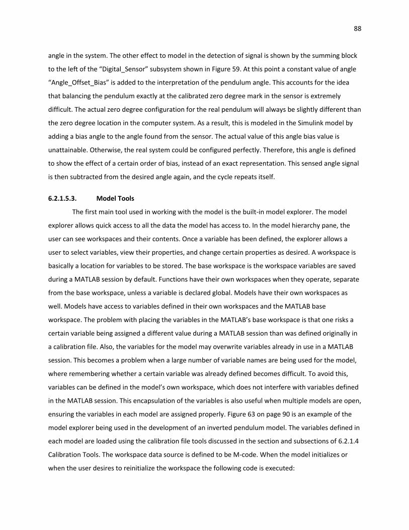
88
angle in the system. The other effect to model in the detection of signal is shown by the summing block
to the left of the “Digital_Sensor” subsystem shown in Figure 59. At this point a constant value of angle
“Angle_Offset_Bias” is added to the interpretation of the pendulum angle. This accounts for the idea
that balancing the pendulum exactly at the calibrated zero degree mark in the sensor is extremely
difficult. The actual zero degree configuration for the real pendulum will always be slightly different than
the zero degree location in the computer system. As a result, this is modeled in the Simulink model by
adding a bias angle to the angle found from the sensor. The actual value of this angle bias value is
unattainable. Otherwise, the real system could be configured perfectly. Therefore, this angle is defined
to show the effect of a certain order of bias, instead of an exact representation. This sensed angle signal
is then subtracted from the desired angle again, and the cycle repeats itself.
6.2.1.5.3. Model Tools
The first main tool used in working with the model is the built-in model explorer. The model
explorer allows quick access to all the data the model has access to. In the model hierarchy pane, the
user can see workspaces and their contents. Once a variable has been defined, the explorer allows a
user to select variables, view their properties, and change certain properties as desired. A workspace is
basically a location for variables to be stored. The base workspace is the workspace variables are saved
during a MATLAB session by default. Functions have their own workspaces when they operate, separate
from the base workspace, unless a variable is declared global. Models have their own workspaces as
well. Models have access to variables defined in their own workspaces and the MATLAB base
workspace. The problem with placing the variables in the MATLAB’s base workspace is that one risks a
certain variable being assigned a different value during a MATLAB session than was defined originally in
a calibration file. Also, the variables for the model may overwrite variables already in use in a MATLAB
session. This becomes a problem when a large number of variable names are being used for the model,
where remembering whether a certain variable was already defined becomes difficult. To avoid this,
variables can be defined in the model’s own workspace, which does not interfere with variables defined
in the MATLAB session. This encapsulation of the variables is also useful when multiple models are open,
ensuring the variables in each model are assigned properly. Figure 63 on page 90 is an example of the
model explorer being used in the development of an inverted pendulum model. The variables defined in
each model are loaded using the calibration file tools discussed in the section and subsections of 6.2.1.4
Calibration Tools. The workspace data source is defined to be M-code. When the model initializes or
when the user desires to reinitialize the workspace the following code is executed:
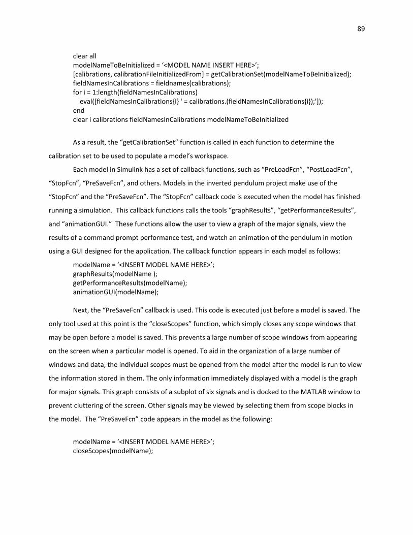
89
clear all modelNameToBeInitialized = ‘<MODEL NAME INSERT HERE>’; [calibrations, calibrationFileInitializedFrom] = getCalibrationSet(modelNameToBeInitialized); fieldNamesInCalibrations = fieldnames(calibrations); for i = 1:length(fieldNamesInCalibrations) eval([fieldNamesInCalibrations{i} ' = calibrations.(fieldNamesInCalibrations{i});']); end clear i calibrations fieldNamesInCalibrations modelNameToBeInitialized
As a result, the “getCalibrationSet” function is called in each function to determine the
calibration set to be used to populate a model’s workspace.
Each model in Simulink has a set of callback functions, such as “PreLoadFcn”, “PostLoadFcn”,
“StopFcn”, “PreSaveFcn”, and others. Models in the inverted pendulum project make use of the
“StopFcn” and the “PreSaveFcn”. The “StopFcn” callback code is executed when the model has finished
running a simulation. This callback functions calls the tools “graphResults”, “getPerformanceResults”,
and “animationGUI.” These functions allow the user to view a graph of the major signals, view the
results of a command prompt performance test, and watch an animation of the pendulum in motion
using a GUI designed for the application. The callback function appears in each model as follows:
modelName = ‘<INSERT MODEL NAME HERE>’; graphResults(modelName ); getPerformanceResults(modelName); animationGUI(modelName); Next, the “PreSaveFcn” callback is used. This code is executed just before a model is saved. The
only tool used at this point is the “closeScopes” function, which simply closes any scope windows that
may be open before a model is saved. This prevents a large number of scope windows from appearing
on the screen when a particular model is opened. To aid in the organization of a large number of
windows and data, the individual scopes must be opened from the model after the model is run to view
the information stored in them. The only information immediately displayed with a model is the graph
for major signals. This graph consists of a subplot of six signals and is docked to the MATLAB window to
prevent cluttering of the screen. Other signals may be viewed by selecting them from scope blocks in
the model. The “PreSaveFcn” code appears in the model as the following:
modelName = ‘<INSERT MODEL NAME HERE>’; closeScopes(modelName);
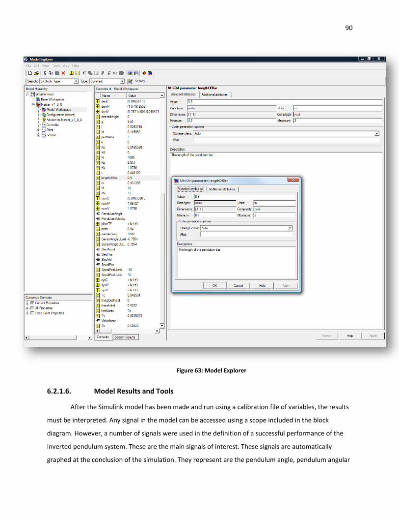
90
Figure 63: Model Explorer
6.2.1.6. Model Results and Tools
After the Simulink model has been made and run using a calibration file of variables, the results
must be interpreted. Any signal in the model can be accessed using a scope included in the block
diagram. However, a number of signals were used in the definition of a successful performance of the
inverted pendulum system. These are the main signals of interest. These signals are automatically
graphed at the conclusion of the simulation. They represent are the pendulum angle, pendulum angular
91
velocity, the sled position, the sled linear velocity, the valve spool command voltage, and the valve spool
linear position. These signals are graphed against their specification limits using the “graphResults”
function called in the Simulink file when the simulation has stopped. Furthermore, these signals are
tested against those performance specifications in a command prompt format using the
“getPerformanceResults” function. This function tests each function, displays the maximum and
minimum values agains the goals, and assess whether the simulation was a “PASS” for success or “FAIL”
for failure. This way, the user can view the overall results graphically from the graphs, and get the
results in numerical form from the command window. Finally, the user can view the results in a third
form using an animation. The “animationGUI” function provides the options for the user to view an
animation from the results at the desired number of frames per second, play speed, and tolerance in
animation error and to save an avi file of the animation for future use. These tools provide the
developer with quick ways to visualize and quantify the results, interpret the data, and asses consistency
in information.
6.2.1.6.1. animationGUI.m
The animation GUI is used to generate an animation of the inverted pendulum results from a
model. The only input to the model is the name of the model that has been run (without the .mdl
extension in the name). However, for the GUI to function properly a number of conditions within
MATLAB must be met before proceeding. First, the object “lengthOfBar” must be defined in the model
workspace with a field “Value” assigned to it. This is the physical length of the pendulum bar. Next, the
object “SledPos” must be defined in the model workspace with fields “Max” and “Min” to define the
allowable stroke of the sled in the system. Next, signals “SledPos” and “PendulumAngle” must be
defined in the model and have been set to data logging. The model must have been run and a structure
“logsout” must exist in the MATLAB base workspace prior to running the model. Finally, the model of
interest must be open so the function can access its workspace for the mentioned objects. This is the
information the function will gather to perform the animation desired by the user.
When the function is run and the requirements mentioned above have been met, a GUI will
appear on the screen in the form shown in Figure 64. If an animation is not desired “Done” may be
selected at any time. Also, this button is pressed when the process is complete. On the right, the
animation may be created using three specifications. First, the speed scale is the playback speed of the
animation. “1.0” means the animation will be played at the real time of the system. “0.5” means the
animation will be played half as fast as real time. And “2.0” means the animation will be played twice as
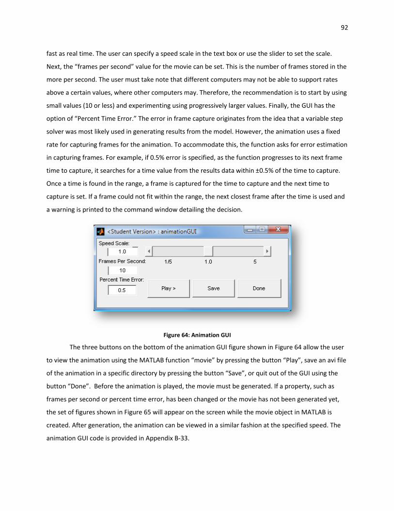
92
fast as real time. The user can specify a speed scale in the text box or use the slider to set the scale.
Next, the “frames per second” value for the movie can be set. This is the number of frames stored in the
more per second. The user must take note that different computers may not be able to support rates
above a certain values, where other computers may. Therefore, the recommendation is to start by using
small values (10 or less) and experimenting using progressively larger values. Finally, the GUI has the
option of “Percent Time Error.” The error in frame capture originates from the idea that a variable step
solver was most likely used in generating results from the model. However, the animation uses a fixed
rate for capturing frames for the animation. To accommodate this, the function asks for error estimation
in capturing frames. For example, if 0.5% error is specified, as the function progresses to its next frame
time to capture, it searches for a time value from the results data within ±0.5% of the time to capture.
Once a time is found in the range, a frame is captured for the time to capture and the next time to
capture is set. If a frame could not fit within the range, the next closest frame after the time is used and
a warning is printed to the command window detailing the decision.
Figure 64: Animation GUI
The three buttons on the bottom of the animation GUI figure shown in Figure 64 allow the user
to view the animation using the MATLAB function “movie” by pressing the button “Play”, save an avi file
of the animation in a specific directory by pressing the button “Save”, or quit out of the GUI using the
button “Done”. Before the animation is played, the movie must be generated. If a property, such as
frames per second or percent time error, has been changed or the movie has not been generated yet,
the set of figures shown in Figure 65 will appear on the screen while the movie object in MATLAB is
created. After generation, the animation can be viewed in a similar fashion at the specified speed. The
animation GUI code is provided in Appendix B-33.
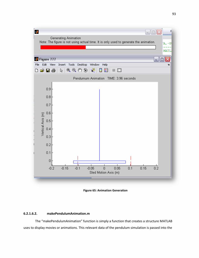
93
Figure 65: Animation Generation
6.2.1.6.2. makePendulumAnimation.m
The “makePendulumAnimation” function is simply a function that creates a structure MATLAB
uses to display movies or animations. This relevant data of the pendulum simulation is passed into the
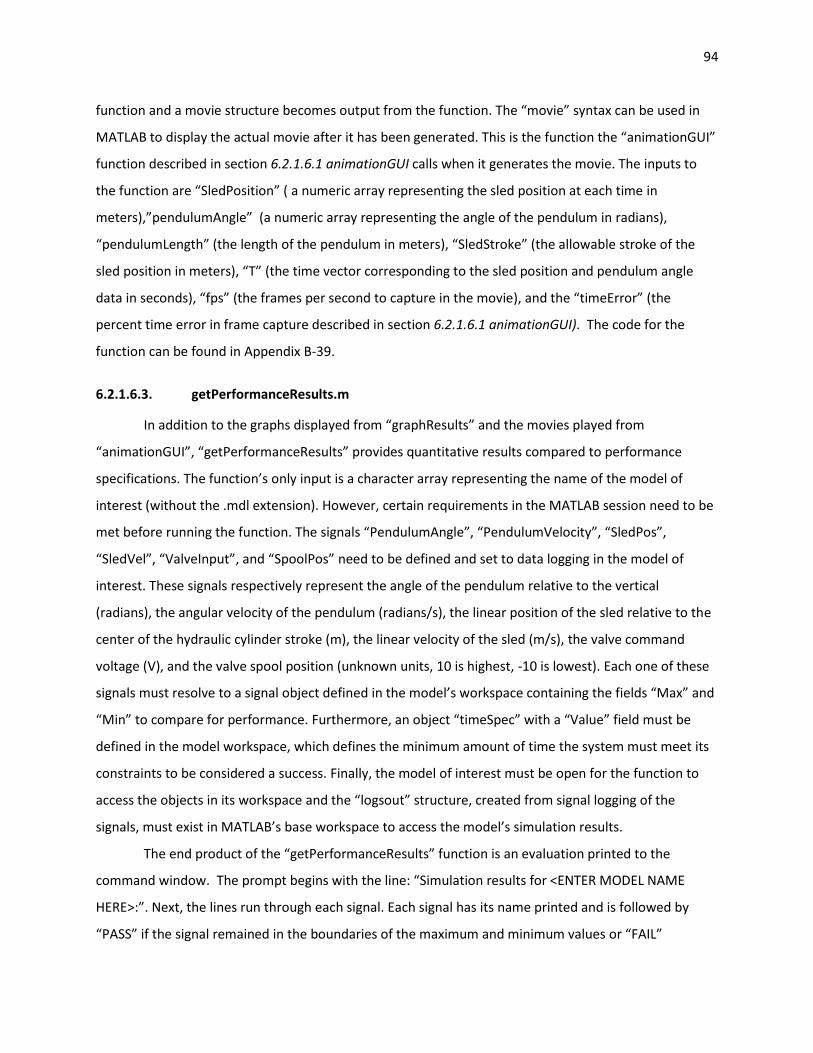
94
function and a movie structure becomes output from the function. The “movie” syntax can be used in
MATLAB to display the actual movie after it has been generated. This is the function the “animationGUI”
function described in section 6.2.1.6.1 animationGUI calls when it generates the movie. The inputs to
the function are “SledPosition” ( a numeric array representing the sled position at each time in
meters),”pendulumAngle” (a numeric array representing the angle of the pendulum in radians),
“pendulumLength” (the length of the pendulum in meters), “SledStroke” (the allowable stroke of the
sled position in meters), “T” (the time vector corresponding to the sled position and pendulum angle
data in seconds), “fps” (the frames per second to capture in the movie), and the “timeError” (the
percent time error in frame capture described in section 6.2.1.6.1 animationGUI). The code for the
function can be found in Appendix B-39.
6.2.1.6.3. getPerformanceResults.m
In addition to the graphs displayed from “graphResults” and the movies played from
“animationGUI”, “getPerformanceResults” provides quantitative results compared to performance
specifications. The function’s only input is a character array representing the name of the model of
interest (without the .mdl extension). However, certain requirements in the MATLAB session need to be
met before running the function. The signals “PendulumAngle”, “PendulumVelocity”, “SledPos”,
“SledVel”, “ValveInput”, and “SpoolPos” need to be defined and set to data logging in the model of
interest. These signals respectively represent the angle of the pendulum relative to the vertical
(radians), the angular velocity of the pendulum (radians/s), the linear position of the sled relative to the
center of the hydraulic cylinder stroke (m), the linear velocity of the sled (m/s), the valve command
voltage (V), and the valve spool position (unknown units, 10 is highest, -10 is lowest). Each one of these
signals must resolve to a signal object defined in the model’s workspace containing the fields “Max” and
“Min” to compare for performance. Furthermore, an object “timeSpec” with a “Value” field must be
defined in the model workspace, which defines the minimum amount of time the system must meet its
constraints to be considered a success. Finally, the model of interest must be open for the function to
access the objects in its workspace and the “logsout” structure, created from signal logging of the
signals, must exist in MATLAB’s base workspace to access the model’s simulation results.
The end product of the “getPerformanceResults” function is an evaluation printed to the
command window. The prompt begins with the line: “Simulation results for <ENTER MODEL NAME
HERE>:”. Next, the lines run through each signal. Each signal has its name printed and is followed by
“PASS” if the signal remained in the boundaries of the maximum and minimum values or “FAIL”
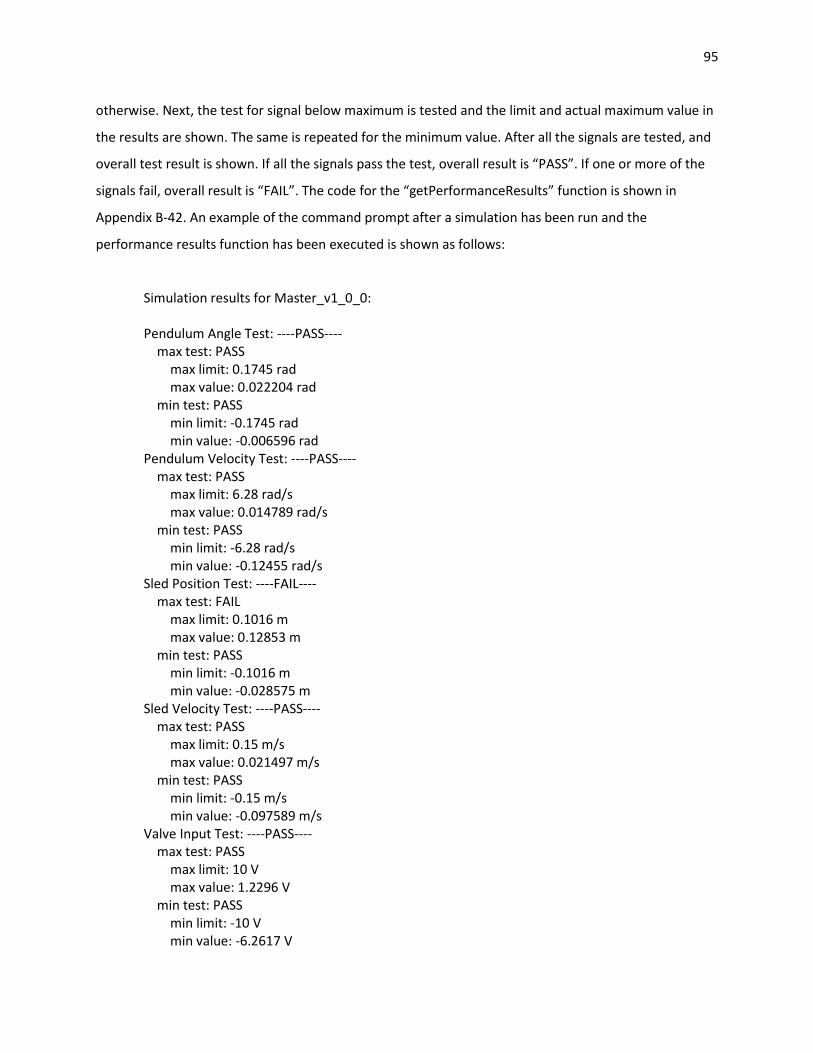
95
otherwise. Next, the test for signal below maximum is tested and the limit and actual maximum value in
the results are shown. The same is repeated for the minimum value. After all the signals are tested, and
overall test result is shown. If all the signals pass the test, overall result is “PASS”. If one or more of the
signals fail, overall result is “FAIL”. The code for the “getPerformanceResults” function is shown in
Appendix B-42. An example of the command prompt after a simulation has been run and the
performance results function has been executed is shown as follows:
Simulation results for Master_v1_0_0: Pendulum Angle Test: ----PASS---- max test: PASS max limit: 0.1745 rad max value: 0.022204 rad min test: PASS min limit: -0.1745 rad min value: -0.006596 rad Pendulum Velocity Test: ----PASS---- max test: PASS max limit: 6.28 rad/s max value: 0.014789 rad/s min test: PASS min limit: -6.28 rad/s min value: -0.12455 rad/s Sled Position Test: ----FAIL---- max test: FAIL max limit: 0.1016 m max value: 0.12853 m min test: PASS min limit: -0.1016 m min value: -0.028575 m Sled Velocity Test: ----PASS---- max test: PASS max limit: 0.15 m/s max value: 0.021497 m/s min test: PASS min limit: -0.15 m/s min value: -0.097589 m/s Valve Input Test: ----PASS---- max test: PASS max limit: 10 V max value: 1.2296 V min test: PASS min limit: -10 V min value: -6.2617 V
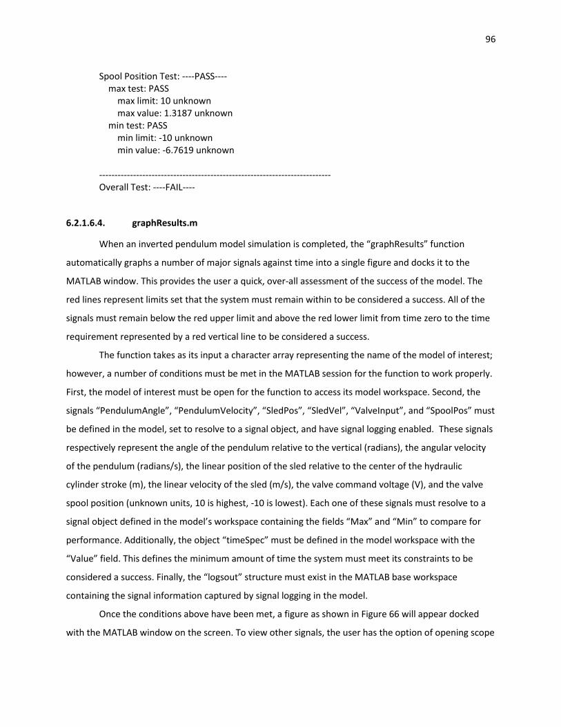
96
Spool Position Test: ----PASS---- max test: PASS max limit: 10 unknown max value: 1.3187 unknown min test: PASS min limit: -10 unknown min value: -6.7619 unknown --------------------------------------------------------------------------- Overall Test: ----FAIL----
6.2.1.6.4. graphResults.m
When an inverted pendulum model simulation is completed, the “graphResults” function
automatically graphs a number of major signals against time into a single figure and docks it to the
MATLAB window. This provides the user a quick, over-all assessment of the success of the model. The
red lines represent limits set that the system must remain within to be considered a success. All of the
signals must remain below the red upper limit and above the red lower limit from time zero to the time
requirement represented by a red vertical line to be considered a success.
The function takes as its input a character array representing the name of the model of interest;
however, a number of conditions must be met in the MATLAB session for the function to work properly.
First, the model of interest must be open for the function to access its model workspace. Second, the
signals “PendulumAngle”, “PendulumVelocity”, “SledPos”, “SledVel”, “ValveInput”, and “SpoolPos” must
be defined in the model, set to resolve to a signal object, and have signal logging enabled. These signals
respectively represent the angle of the pendulum relative to the vertical (radians), the angular velocity
of the pendulum (radians/s), the linear position of the sled relative to the center of the hydraulic
cylinder stroke (m), the linear velocity of the sled (m/s), the valve command voltage (V), and the valve
spool position (unknown units, 10 is highest, -10 is lowest). Each one of these signals must resolve to a
signal object defined in the model’s workspace containing the fields “Max” and “Min” to compare for
performance. Additionally, the object “timeSpec” must be defined in the model workspace with the
“Value” field. This defines the minimum amount of time the system must meet its constraints to be
considered a success. Finally, the “logsout” structure must exist in the MATLAB base workspace
containing the signal information captured by signal logging in the model.
Once the conditions above have been met, a figure as shown in Figure 66 will appear docked
with the MATLAB window on the screen. To view other signals, the user has the option of opening scope
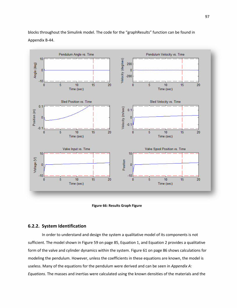
97
blocks throughout the Simulink model. The code for the “graphResults” function can be found in
Appendix B-44.
Figure 66: Results Graph Figure
6.2.2. System Identification
In order to understand and design the system a qualitative model of its components is not
sufficient. The model shown in Figure 59 on page 85, Equation 1, and Equation 2 provides a qualitative
form of the valve and cylinder dynamics within the system. Figure 61 on page 86 shows calculations for
modeling the pendulum. However, unless the coefficients in these equations are known, the model is
useless. Many of the equations for the pendulum were derived and can be seen in Appendix A:
Equations. The masses and inertias were calculated using the known densities of the materials and the
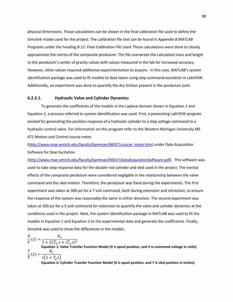
98
physical dimensions. Those calculations can be shown in the final calibration file used to define the
Simulink model used for the project. The calibration file text can be found in Appendix B:MATLAB
Programs under the heading B 12: Final Calibration File Used. These calculations were done to closely
approximate the inertia of the composite pendulum. The file overwrote the calculated mass and length
to the pendulum’s center of gravity values with values measured in the lab for increased accuracy.
However, other values required additional experimentation to acquire. In this case, MATLAB’s system
identification package was used to fit models to data taken using step command excitation in LabVIEW.
Additionally, an experiment was done to quantify the dry friction present in the pendulum joint.
6.2.2.1. Hydraulic Valve and Cylinder Dynamics
To generate the coefficients of the models in the Laplace domain shown in Equation 1 and
Equation 2, a process referred to system identification was used. First, a preexisting LabVIEW program
existed for generating the position response of a hydraulic cylinder to a step voltage command to a
hydraulic control valve. For information on this program refer to the Western Michigan University ME
471 Motion and Control course notes
(http://www.mae.wmich.edu/faculty/kamman/ME471course_notes.htm) under Data Acquisition
Software for Step Excitation
(http://www.mae.wmich.edu/faculty/kamman/ME471DataAcquisitionSoftware.pdf). This software was
used to take step response data for the double-rod cylinder and sled used in the project. The inertial
effects of the composite pendulum were considered negligible in the relationship between the valve
command and the sled motion. Therefore, the pendulum was fixed during the experiments. The first
experiment was taken at 300 psi for a 7 volt command, both during extension and retraction, to ensure
the response of the system was reasonably the same in either direction. The second experiment was
taken at 500 psi for a 5 volt command for extension to quantify the valve and cylinder dynamics at the
conditions used in the project. Next, the system identification package in MATLAB was used to fit the
models in Equation 1 and Equation 2 to the experimental data and generate the coefficients. Finally,
Simulink was used to show the differences in the models.
𝑋
𝑉 𝑠 =
𝐾𝑣1 + 2𝜁𝑇𝑤𝑠 + 𝑇𝑤𝑠
2
Equation 1: Valve Transfer Function Model (X is spool position, and V is command voltage in volts) 𝑌
𝑋 𝑠 =
𝐾𝑐
𝑠 1 + 𝑇𝑝𝑠
Equation 2: Cylinder Transfer Function Model (X is spool position, and Y is sled position in inches)
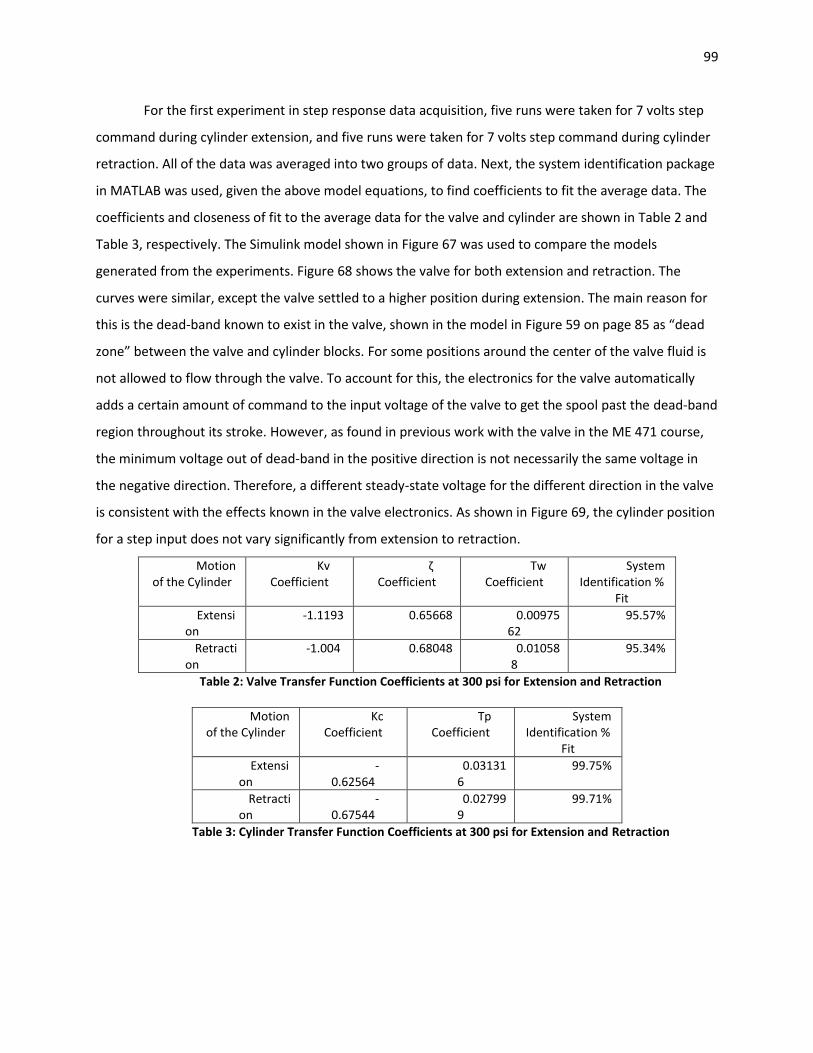
99
For the first experiment in step response data acquisition, five runs were taken for 7 volts step
command during cylinder extension, and five runs were taken for 7 volts step command during cylinder
retraction. All of the data was averaged into two groups of data. Next, the system identification package
in MATLAB was used, given the above model equations, to find coefficients to fit the average data. The
coefficients and closeness of fit to the average data for the valve and cylinder are shown in Table 2 and
Table 3, respectively. The Simulink model shown in Figure 67 was used to compare the models
generated from the experiments. Figure 68 shows the valve for both extension and retraction. The
curves were similar, except the valve settled to a higher position during extension. The main reason for
this is the dead-band known to exist in the valve, shown in the model in Figure 59 on page 85 as “dead
zone” between the valve and cylinder blocks. For some positions around the center of the valve fluid is
not allowed to flow through the valve. To account for this, the electronics for the valve automatically
adds a certain amount of command to the input voltage of the valve to get the spool past the dead-band
region throughout its stroke. However, as found in previous work with the valve in the ME 471 course,
the minimum voltage out of dead-band in the positive direction is not necessarily the same voltage in
the negative direction. Therefore, a different steady-state voltage for the different direction in the valve
is consistent with the effects known in the valve electronics. As shown in Figure 69, the cylinder position
for a step input does not vary significantly from extension to retraction.
Motion of the Cylinder
Kv Coefficient
ζ Coefficient
Tw Coefficient
System Identification %
Fit
Extension
-1.1193 0.65668 0.0097562
95.57%
Retraction
-1.004 0.68048 0.010588
95.34%
Table 2: Valve Transfer Function Coefficients at 300 psi for Extension and Retraction
Motion
of the Cylinder Kc
Coefficient Tp
Coefficient System
Identification % Fit
Extension
-0.62564
0.031316
99.75%
Retraction
-0.67544
0.027999
99.71%
Table 3: Cylinder Transfer Function Coefficients at 300 psi for Extension and Retraction
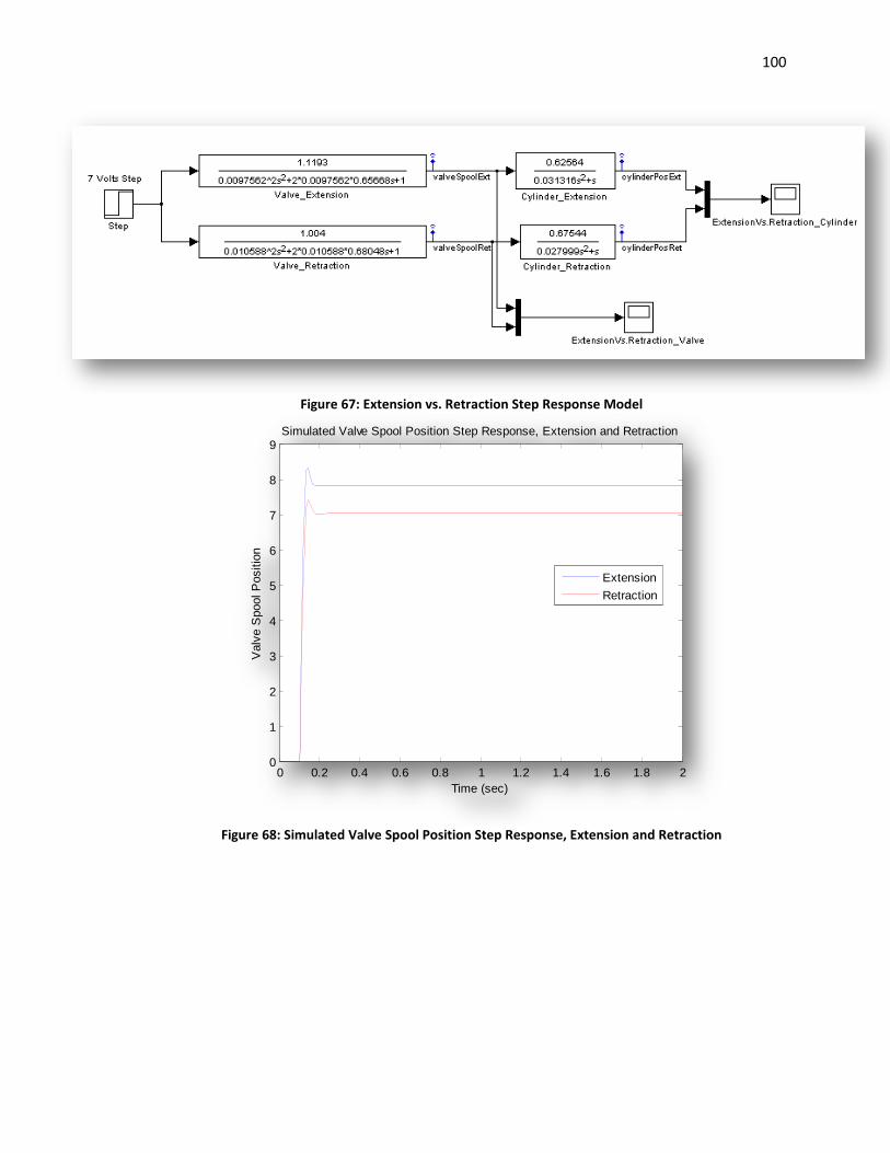
100
Figure 67: Extension vs. Retraction Step Response Model
Figure 68: Simulated Valve Spool Position Step Response, Extension and Retraction
0 0.2 0.4 0.6 0.8 1 1.2 1.4 1.6 1.8 20
1
2
3
4
5
6
7
8
9Simulated Valve Spool Position Step Response, Extension and Retraction
Time (sec)
Valv
e S
pool P
ositio
n
Extension
Retraction
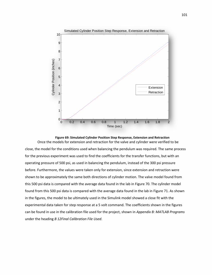
101
Figure 69: Simulated Cylinder Position Step Response, Extension and Retraction
Once the models for extension and retraction for the valve and cylinder were verified to be
close, the model for the conditions used when balancing the pendulum was required. The same process
for the previous experiment was used to find the coefficients for the transfer functions, but with an
operating pressure of 500 psi, as used in balancing the pendulum, instead of the 300 psi pressure
before. Furthermore, the values were taken only for extension, since extension and retraction were
shown to be approximately the same both directions of cylinder motion. The valve model found from
this 500 psi data is compared with the average data found in the lab in Figure 70. The cylinder model
found from this 500 psi data is compared with the average data found in the lab in Figure 71. As shown
in the figures, the model to be ultimately used in the Simulink model showed a close fit with the
experimental data taken for step response at a 5 volt command. The coefficients shown in the figures
can be found in use in the calibration file used for the project, shown in Appendix B: MATLAB Programs
under the heading B 12Final Calibration File Used.
0 0.2 0.4 0.6 0.8 1 1.2 1.4 1.6 1.8 20
1
2
3
4
5
6
7
8
9
10Simulated Cylinder Position Step Response, Extension and Retraction
Time (sec)
Cylin
der
Positio
n (
inches)
Extension
Retraction
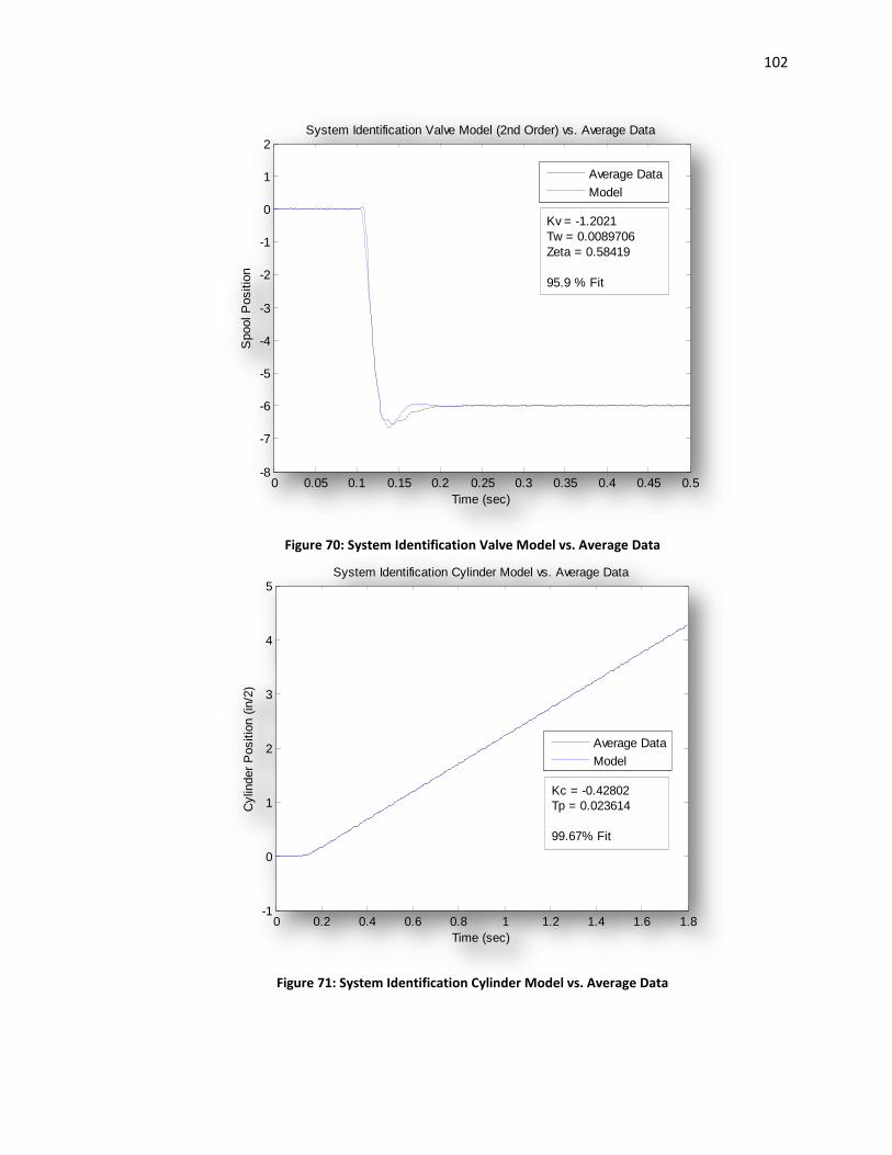
102
Figure 70: System Identification Valve Model vs. Average Data
Figure 71: System Identification Cylinder Model vs. Average Data
0 0.05 0.1 0.15 0.2 0.25 0.3 0.35 0.4 0.45 0.5-8
-7
-6
-5
-4
-3
-2
-1
0
1
2
Time (sec)
Spool P
ositio
n
System Identification Valve Model (2nd Order) vs. Average Data
Average Data
Model
Kv = -1.2021
Tw = 0.0089706
Zeta = 0.58419
95.9 % Fit
0 0.2 0.4 0.6 0.8 1 1.2 1.4 1.6 1.8-1
0
1
2
3
4
5
Time (sec)
Cylin
der
Positio
n (
in/2
)
System Identification Cylinder Model vs. Average Data
Average Data
Model
Kc = -0.42802
Tp = 0.023614
99.67% Fit
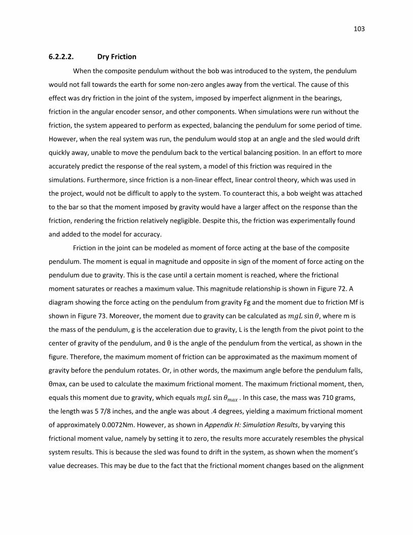
103
6.2.2.2. Dry Friction
When the composite pendulum without the bob was introduced to the system, the pendulum
would not fall towards the earth for some non-zero angles away from the vertical. The cause of this
effect was dry friction in the joint of the system, imposed by imperfect alignment in the bearings,
friction in the angular encoder sensor, and other components. When simulations were run without the
friction, the system appeared to perform as expected, balancing the pendulum for some period of time.
However, when the real system was run, the pendulum would stop at an angle and the sled would drift
quickly away, unable to move the pendulum back to the vertical balancing position. In an effort to more
accurately predict the response of the real system, a model of this friction was required in the
simulations. Furthermore, since friction is a non-linear effect, linear control theory, which was used in
the project, would not be difficult to apply to the system. To counteract this, a bob weight was attached
to the bar so that the moment imposed by gravity would have a larger affect on the response than the
friction, rendering the friction relatively negligible. Despite this, the friction was experimentally found
and added to the model for accuracy.
Friction in the joint can be modeled as moment of force acting at the base of the composite
pendulum. The moment is equal in magnitude and opposite in sign of the moment of force acting on the
pendulum due to gravity. This is the case until a certain moment is reached, where the frictional
moment saturates or reaches a maximum value. This magnitude relationship is shown in Figure 72. A
diagram showing the force acting on the pendulum from gravity Fg and the moment due to friction Mf is
shown in Figure 73. Moreover, the moment due to gravity can be calculated as 𝑚𝑔𝐿 sin𝜃, where m is
the mass of the pendulum, g is the acceleration due to gravity, L is the length from the pivot point to the
center of gravity of the pendulum, and θ is the angle of the pendulum from the vertical, as shown in the
figure. Therefore, the maximum moment of friction can be approximated as the maximum moment of
gravity before the pendulum rotates. Or, in other words, the maximum angle before the pendulum falls,
θmax, can be used to calculate the maximum frictional moment. The maximum frictional moment, then,
equals this moment due to gravity, which equals 𝑚𝑔𝐿 sin𝜃𝑚𝑎𝑥 . In this case, the mass was 710 grams,
the length was 5 7/8 inches, and the angle was about .4 degrees, yielding a maximum frictional moment
of approximately 0.0072Nm. However, as shown in Appendix H: Simulation Results, by varying this
frictional moment value, namely by setting it to zero, the results more accurately resembles the physical
system results. This is because the sled was found to drift in the system, as shown when the moment’s
value decreases. This may be due to the fact that the frictional moment changes based on the alignment
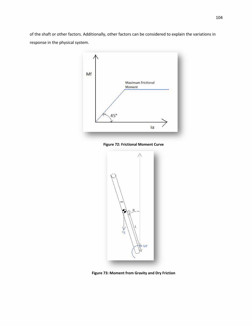
104
of the shaft or other factors. Additionally, other factors can be considered to explain the variations in
response in the physical system.
Figure 72: Frictional Moment Curve
Figure 73: Moment from Gravity and Dry Friction
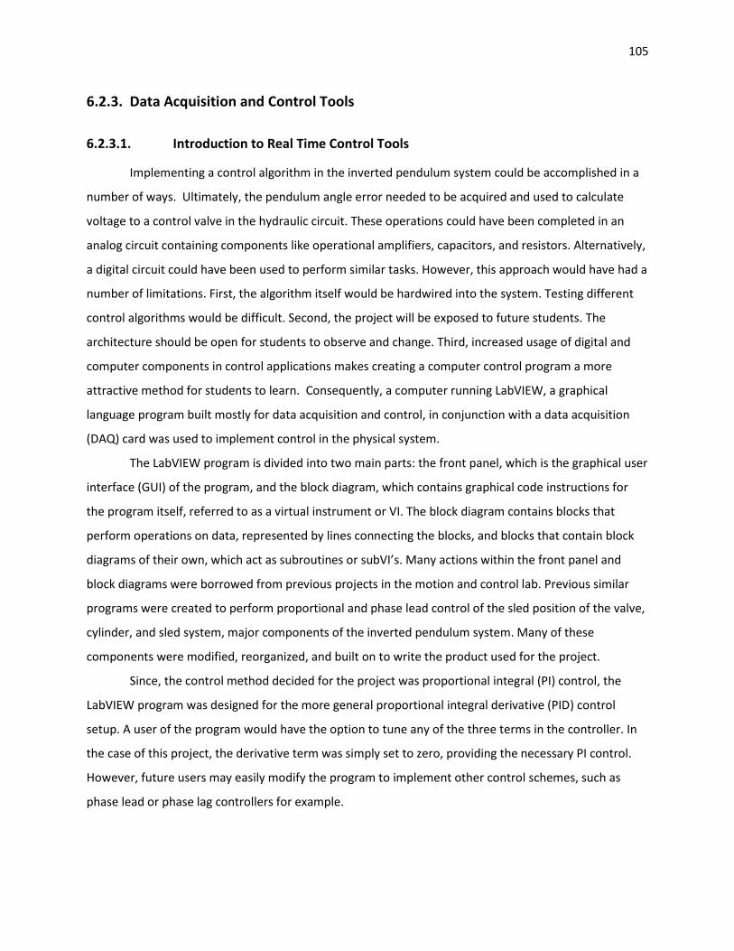
105
6.2.3. Data Acquisition and Control Tools
6.2.3.1. Introduction to Real Time Control Tools
Implementing a control algorithm in the inverted pendulum system could be accomplished in a
number of ways. Ultimately, the pendulum angle error needed to be acquired and used to calculate
voltage to a control valve in the hydraulic circuit. These operations could have been completed in an
analog circuit containing components like operational amplifiers, capacitors, and resistors. Alternatively,
a digital circuit could have been used to perform similar tasks. However, this approach would have had a
number of limitations. First, the algorithm itself would be hardwired into the system. Testing different
control algorithms would be difficult. Second, the project will be exposed to future students. The
architecture should be open for students to observe and change. Third, increased usage of digital and
computer components in control applications makes creating a computer control program a more
attractive method for students to learn. Consequently, a computer running LabVIEW, a graphical
language program built mostly for data acquisition and control, in conjunction with a data acquisition
(DAQ) card was used to implement control in the physical system.
The LabVIEW program is divided into two main parts: the front panel, which is the graphical user
interface (GUI) of the program, and the block diagram, which contains graphical code instructions for
the program itself, referred to as a virtual instrument or VI. The block diagram contains blocks that
perform operations on data, represented by lines connecting the blocks, and blocks that contain block
diagrams of their own, which act as subroutines or subVI’s. Many actions within the front panel and
block diagrams were borrowed from previous projects in the motion and control lab. Previous similar
programs were created to perform proportional and phase lead control of the sled position of the valve,
cylinder, and sled system, major components of the inverted pendulum system. Many of these
components were modified, reorganized, and built on to write the product used for the project.
Since, the control method decided for the project was proportional integral (PI) control, the
LabVIEW program was designed for the more general proportional integral derivative (PID) control
setup. A user of the program would have the option to tune any of the three terms in the controller. In
the case of this project, the derivative term was simply set to zero, providing the necessary PI control.
However, future users may easily modify the program to implement other control schemes, such as
phase lead or phase lag controllers for example.
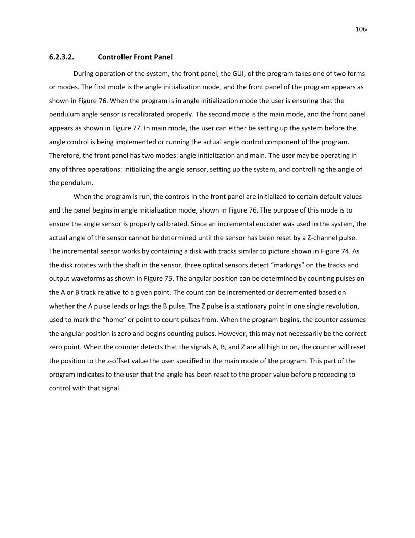
106
6.2.3.2. Controller Front Panel
During operation of the system, the front panel, the GUI, of the program takes one of two forms
or modes. The first mode is the angle initialization mode, and the front panel of the program appears as
shown in Figure 76. When the program is in angle initialization mode the user is ensuring that the
pendulum angle sensor is recalibrated properly. The second mode is the main mode, and the front panel
appears as shown in Figure 77. In main mode, the user can either be setting up the system before the
angle control is being implemented or running the actual angle control component of the program.
Therefore, the front panel has two modes: angle initialization and main. The user may be operating in
any of three operations: initializing the angle sensor, setting up the system, and controlling the angle of
the pendulum.
When the program is run, the controls in the front panel are initialized to certain default values
and the panel begins in angle initialization mode, shown in Figure 76. The purpose of this mode is to
ensure the angle sensor is properly calibrated. Since an incremental encoder was used in the system, the
actual angle of the sensor cannot be determined until the sensor has been reset by a Z-channel pulse.
The incremental sensor works by containing a disk with tracks similar to picture shown in Figure 74. As
the disk rotates with the shaft in the sensor, three optical sensors detect “markings” on the tracks and
output waveforms as shown in Figure 75. The angular position can be determined by counting pulses on
the A or B track relative to a given point. The count can be incremented or decremented based on
whether the A pulse leads or lags the B pulse. The Z pulse is a stationary point in one single revolution,
used to mark the “home” or point to count pulses from. When the program begins, the counter assumes
the angular position is zero and begins counting pulses. However, this may not necessarily be the correct
zero point. When the counter detects that the signals A, B, and Z are all high or on, the counter will reset
the position to the z-offset value the user specified in the main mode of the program. This part of the
program indicates to the user that the angle has been reset to the proper value before proceeding to
control with that signal.
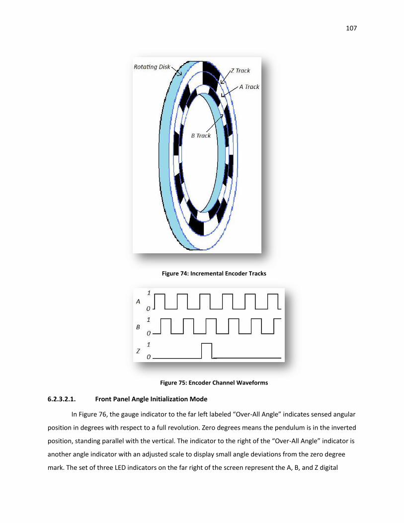
107
Figure 74: Incremental Encoder Tracks
Figure 75: Encoder Channel Waveforms
6.2.3.2.1. Front Panel Angle Initialization Mode
In Figure 76, the gauge indicator to the far left labeled “Over-All Angle” indicates sensed angular
position in degrees with respect to a full revolution. Zero degrees means the pendulum is in the inverted
position, standing parallel with the vertical. The indicator to the right of the “Over-All Angle” indicator is
another angle indicator with an adjusted scale to display small angle deviations from the zero degree
mark. The set of three LED indicators on the far right of the screen represent the A, B, and Z digital
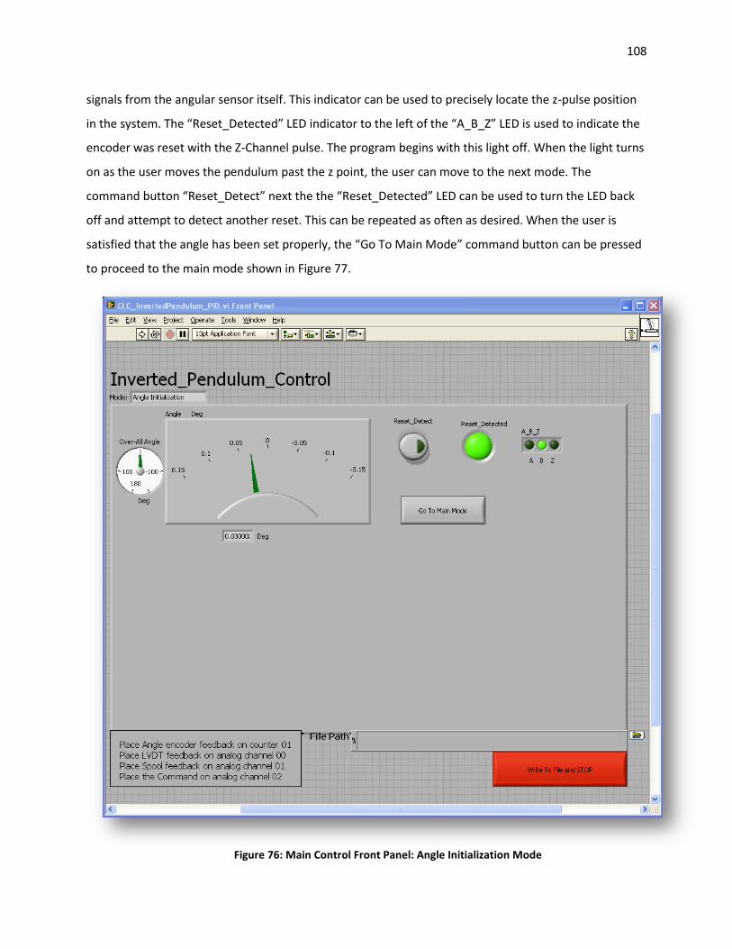
108
signals from the angular sensor itself. This indicator can be used to precisely locate the z-pulse position
in the system. The “Reset_Detected” LED indicator to the left of the “A_B_Z” LED is used to indicate the
encoder was reset with the Z-Channel pulse. The program begins with this light off. When the light turns
on as the user moves the pendulum past the z point, the user can move to the next mode. The
command button “Reset_Detect” next the the “Reset_Detected” LED can be used to turn the LED back
off and attempt to detect another reset. This can be repeated as often as desired. When the user is
satisfied that the angle has been set properly, the “Go To Main Mode” command button can be pressed
to proceed to the main mode shown in Figure 77.
Figure 76: Main Control Front Panel: Angle Initialization Mode
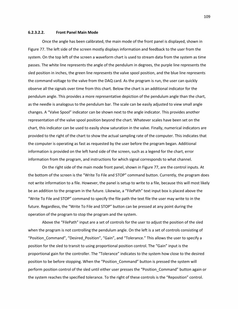
109
6.2.3.2.2. Front Panel Main Mode
Once the angle has been calibrated, the main mode of the front panel is displayed, shown in
Figure 77. The left side of the screen mostly displays information and feedback to the user from the
system. On the top left of the screen a waveform chart is used to stream data from the system as time
passes. The white line represents the angle of the pendulum in degrees, the purple line represents the
sled position in inches, the green line represents the valve spool position, and the blue line represents
the command voltage to the valve from the DAQ card. As the program is run, the user can quickly
observe all the signals over time from this chart. Below the chart is an additional indicator for the
pendulum angle. This provides a more representative depiction of the pendulum angle than the chart,
as the needle is analogous to the pendulum bar. The scale can be easily adjusted to view small angle
changes. A “Valve Spool” indicator can be shown next to the angle indicator. This provides another
representation of the valve spool position beyond the chart. Whatever scales have been set on the
chart, this indicator can be used to easily show saturation in the valve. Finally, numerical indicators are
provided to the right of the chart to show the actual sampling rate of the computer. This indicates that
the computer is operating as fast as requested by the user before the program began. Additional
information is provided on the left hand side of the screen, such as a legend for the chart, error
information from the program, and instructions for which signal corresponds to what channel.
On the right side of the main mode front panel, shown in Figure 77, are the control inputs. At
the bottom of the screen is the “Write To File and STOP” command button. Currently, the program does
not write information to a file. However, the panel is setup to write to a file, because this will most likely
be an addition to the program in the future. Likewise, a “FilePath” text input box is placed above the
“Write To File and STOP” command to specify the file path the text file the user may write to in the
future. Regardless, the “Write To File and STOP” button can be pressed at any point during the
operation of the program to stop the program and the system.
Above the “FilePath” input are a set of controls for the user to adjust the position of the sled
when the program is not controlling the pendulum angle. On the left is a set of controls consisting of
“Position_Command”, “Desired_Position”, “Gain”, and “Tolerance.” This allows the user to specify a
position for the sled to transit to using proportional position control. The “Gain” input is the
proportional gain for the controller. The “Tolerance” indicates to the system how close to the desired
position to be before stopping. When the “Position_Command” button is pressed the system will
perform position control of the sled until either user presses the “Position_Command” button again or
the system reaches the specified tolerance. To the right of these controls is the “Reposition” control.
110
This provides an alternative to the sled position control for adjusting the sled. The slider can be moved
or a value can be specified in the numerical control to directly command a voltage to the valve, which
moves the cylinder by directing hydraulic flow into its ports. These controls allow the user to set up the
initial conditions of the sled before angle control is attempted, when the green “Control” button at the
top of the screen is off.
Above the cylinder position setup controls are the sample timing and z-offset controls. All inputs
on the front panel can be changed while the program is running, except the sample timing and z-offset
controls. These settings must be set before the program is run. The “Sample_Rate” input is the desired
sample rate of the system in Hz. This is the rate the system gets input from the sensors, calculates
outputs, and sends output. The actual sampling rate of the system is shown to the right of the input, and
the sample period is provided below the input. The “Z_initial” and “Initial_Multiplier” are used in
conjunction to set the angular position when the encoder resets its value with the Z-channel pulse. The
angular position the encoder is set to at reset, the “home”, is equivalent to the “Z_initial” value
multiplied by the “Initial_Multiplier” value in degrees. For more information on the z-offset value refer
to sections 6.2.3.2: Controller Front Panel and 6.2.3.2.1: Front Panel Angle Initialization Mode.
Next, the angle controller inputs can be found above the z-offset input. This is where the user
can tune the PID controller used to control the pendulum angle when the green “Control” button at the
top of the screen is on. The user can change these coefficients when the pendulum angle is not being
controlled. To the right of the PID coefficient inputs are the limit inputs. These values can be set before
control is implemented to automatically stop controller the pendulum when certain conditions are met.
The “Angle_Limit” input specifies the maximum magnitude of angle away from the vertical the
pendulum must be before the program stops control. The “Sled_Max” and “Sled_Min” inputs define the
range of sled position the sled must be within before angle control is terminated. This can be used to
prevent the sled from actually moving to the extremes of its physical stroke. These limits can be set for
safety or for test validity. For instance, if the feet on the pendulum were set at ±0.5 degrees the
program’s angle limit can be set to 0.51 or 0.52 degrees. When the program is controlling the angle, if
the feet actually touch the sled the program will stop the control. This can be used to ensure the
pendulum is being legitimately stabilized by the control, not by bouncing off the sled by the feet.
Finally, the last input is the green “Control” button found at the top right of the screen. When
the button is off or dim, the user can adjust the settings of the system (except sample rate and z-offset)
and reposition the sled. When this control is activated, it will light up, and system will control the
angular position of the inverted pendulum. At this time, only the angle and sled position limits may be
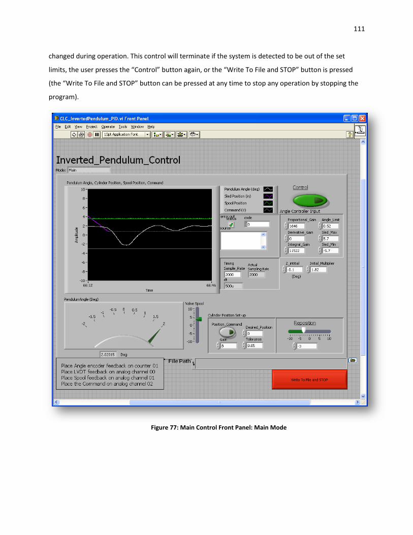
111
changed during operation. This control will terminate if the system is detected to be out of the set
limits, the user presses the “Control” button again, or the “Write To File and STOP” button is pressed
(the “Write To File and STOP” button can be pressed at any time to stop any operation by stopping the
program).
Figure 77: Main Control Front Panel: Main Mode

112
6.2.3.3. Controller Block Diagram
One of the main reasons for using LabVIEW over other methods of control implementation was
the exposure of the logic behind the application. LabVIEW facilitates a graphical approach to
programming. Instead of using commands in a text format, LabVIEW allows programmers to design in a
block diagram. These block diagrams aid other developers to easily understand the logic flow of a
coworker’s work. The inverted pendulum control block diagram has been divided into several subVI’s to
make the program less cluttered and more understandable. The structure has a main diagram for the
entire program that calls a number of smaller block diagrams to perform specific tasks. The main VI is
labeled “CLC_InvertedPendulum_PID.vi” for closed loop control of the inverted pendulum using PID
control. The main VI uses 7 other subVI’s within its block diagram to perform the tasks discussed in the
sections and subsections of 6.2.3.2: Controller Front Panel.
The subVI’s used in the program are “AIVoltageTask.vi”, “CalculatePIDEqCoefficients.vi”,
“DigitalInputTask.vi”, “EncoderTask.vi”, “PackageInputData.vi”, “PIDController.vi”, and
“ProportionalControl.vi.” The “AIVoltageTask.vi” creates a channel containing the analog voltage input
signals (command voltage, valve spool LVDT voltage, and sled position LVDT voltage) timed at the
specified sample rate. The block diagram can be found on page Appendix D-1. The
“CalculatePIDEqCoefficients.vi” calculates the coefficients to the difference equation used to represent
the PID controller as a function of the PID coefficients and the actual sample period. The block diagram
can be found on page Appendix D-2. The “DigitalInputTask.vi”, whose block diagram can be found on
page Appendix D-3, creates a digital channel to detect the pulses from the encoder directly. This digital
task is used to verify z reset in the program during the angle initialization mode discussed in section
6.2.3.2.1: Front Panel Angle Initialization Mode. The “EncoderTask.vi” creates the task to detect the
angular position of pendulum using the incremental encoder. This block diagram can be found on page
Appendix D-4. The “PackageInputData.vi”, shown on page Appendix D-5, removes clutter from the main
block diagram by packing and unpacking signal data from the analog and encoder arrays to be used
within the main while loop in the main program. The “PIDController.vi” is the subVI that actually
implements the difference equation that represents the PID controller and determines if the controller
should stop based on position limits. The block diagram can be found on page Appendix D-6. The
“ProportionalControl.vi” subVI is used to perform the proportional control of the sled position for the
user to reposition the sled before initiated the angle control. The block diagram can be found on page
Appendix D-7. The front panels for these VI’s serve only to define the inputs and outputs of the subVI to
be used by another block diagram. Each subVI front panel appears similar what is shown in Figure 78.
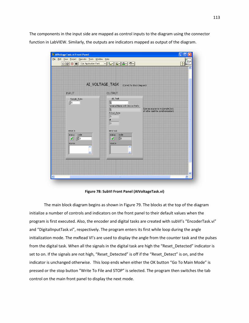
113
The components in the input side are mapped as control inputs to the diagram using the connector
function in LabVIEW. Similarly, the outputs are indicators mapped as output of the diagram.
Figure 78: SubVI Front Panel (AIVoltageTask.vi)
The main block diagram begins as shown in Figure 79. The blocks at the top of the diagram
initialize a number of controls and indicators on the front panel to their default values when the
program is first executed. Also, the encoder and digital tasks are created with subVI’s “EncoderTask.vi”
and “DigitalInputTask.vi”, respectively. The program enters its first while loop during the angle
initialization mode. The mxRead VI’s are used to display the angle from the counter task and the pulses
from the digital task. When all the signals in the digital task are high the “Reset_Detected” indicator is
set to on. If the signals are not high, “Reset_Detected” is off if the “Reset_Detect” is on, and the
indicator is unchanged otherwise. This loop ends when either the OK button “Go To Main Mode” is
pressed or the stop button “Write To File and STOP” is selected. The program then switches the tab
control on the main front panel to display the next mode.
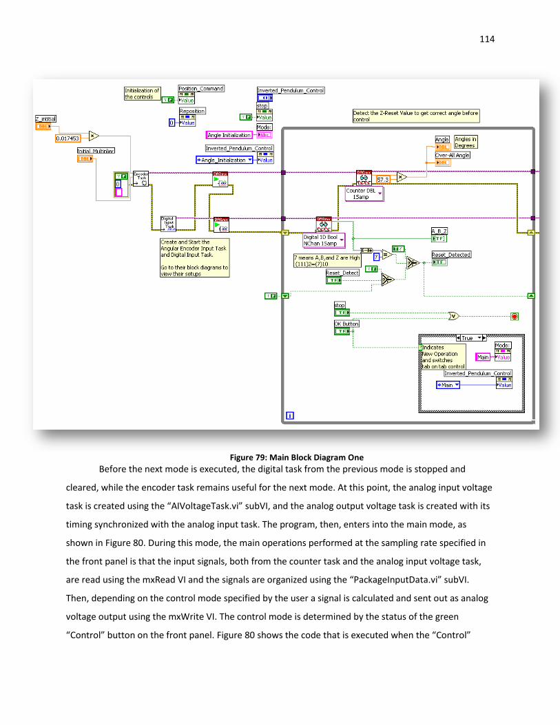
114
Figure 79: Main Block Diagram One
Before the next mode is executed, the digital task from the previous mode is stopped and
cleared, while the encoder task remains useful for the next mode. At this point, the analog input voltage
task is created using the “AIVoltageTask.vi” subVI, and the analog output voltage task is created with its
timing synchronized with the analog input task. The program, then, enters into the main mode, as
shown in Figure 80. During this mode, the main operations performed at the sampling rate specified in
the front panel is that the input signals, both from the counter task and the analog input voltage task,
are read using the mxRead VI and the signals are organized using the “PackageInputData.vi” subVI.
Then, depending on the control mode specified by the user a signal is calculated and sent out as analog
voltage output using the mxWrite VI. The control mode is determined by the status of the green
“Control” button on the front panel. Figure 80 shows the code that is executed when the “Control”
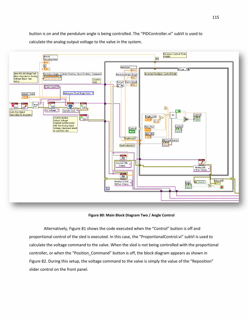
115
button is on and the pendulum angle is being controlled. The “PIDController.vi” subVI is used to
calculate the analog output voltage to the valve in the system.
Figure 80: Main Block Diagram Two / Angle Control
Alternatively, Figure 81 shows the code executed when the “Control” button is off and
proportional control of the sled is executed. In this case, the “ProportionalControl.vi” subVI is used to
calculate the voltage command to the valve. When the sled is not being controlled with the proportional
controller, or when the “Position_Command” button is off, the block diagram appears as shown in
Figure 82. During this setup, the voltage command to the valve is simply the value of the “Reposition”
slider control on the front panel.
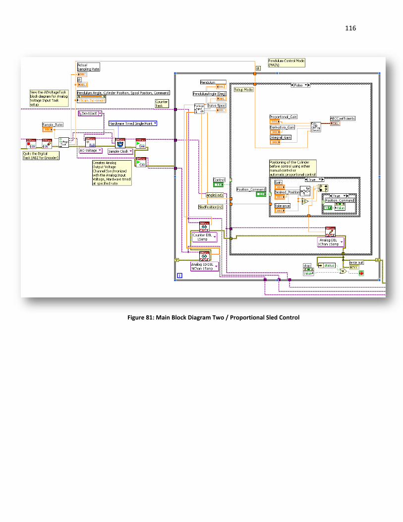
116
Figure 81: Main Block Diagram Two / Proportional Sled Control
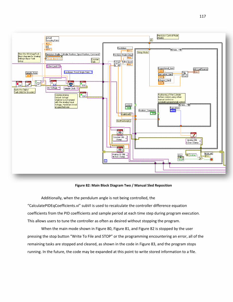
117
Figure 82: Main Block Diagram Two / Manual Sled Reposition
Additionally, when the pendulum angle is not being controlled, the
“CalculatePIDEqCoefficients.vi” subVI is used to recalculate the controller difference equation
coefficients from the PID coefficients and sample period at each time step during program execution.
This allows users to tune the controller as often as desired without stopping the program.
When the main mode shown in Figure 80, Figure 81, and Figure 82 is stopped by the user
pressing the stop button “Write To File and STOP” or the programming encountering an error, all of the
remaining tasks are stopped and cleared, as shown in the code in Figure 83, and the program stops
running. In the future, the code may be expanded at this point to write stored information to a file.
118
Figure 83: Main Block Diagram Three
6.2.4. Controller Design
6.2.4.1. Open Loop System
The first step in performing a control design analysis for a closed loop system is to characterize
the open loop system. A basic model of the closed loop system is shown in Figure 58 on page 83. The
open loop transfer function consists of the part of the diagram from the angle error to the pendulum
angle signal, without the summing block and desired angle. The valve and cylinder models defined in the
Laplace domain have been found in section 6.2.2.1: Hydraulic Valve and Cylinder Dynamics to be a
second order function without zeros and a first order function with a zero, respectively. The coefficients
found during the system identification process placed two complex poles from the valve at
approximately -65±90i and a real pole and zero from the cylinder at about -42 and 0. The unstable
pendulum model derived in Equation 30 in Appendix A-4, neglecting any stiffness or damping in the
joint, contributes real poles at about ±3.3. At this point, the root locus diagram appears as shown in
Figure 84. The figure does not show the valve poles far in the left hand plane to emphasize the more
dominant branches near the origin. As shown in the figure, the system will be unstable for any
proportional gain placed in the system. A pole will always exist in the unstable right hand plane and will
dominate the response of the system, as the pole is relatively close to the origin at any point. At this
point, compensation beyond proportional control is required.
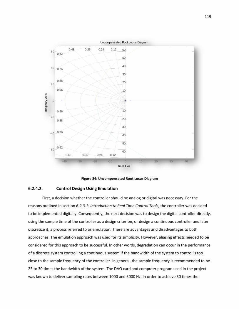
119
Figure 84: Uncompensated Root Locus Diagram
6.2.4.2. Control Design Using Emulation
First, a decision whether the controller should be analog or digital was necessary. For the
reasons outlined in section 6.2.3.1: Introduction to Real Time Control Tools, the controller was decided
to be implemented digitally. Consequently, the next decision was to design the digital controller directly,
using the sample time of the controller as a design criterion, or design a continuous controller and later
discretize it, a process referred to as emulation. There are advantages and disadvantages to both
approaches. The emulation approach was used for its simplicity. However, aliasing effects needed to be
considered for this approach to be successful. In other words, degradation can occur in the performance
of a discrete system controlling a continuous system if the bandwidth of the system to control is too
close to the sample frequency of the controller. In general, the sample frequency is recommended to be
25 to 30 times the bandwidth of the system. The DAQ card and computer program used in the project
was known to deliver sampling rates between 1000 and 3000 Hz. In order to achieve 30 times the
Uncompensated Root Locus Diagram
Real Axis
Imagin
ary
Axis
-40 -30 -20 -10 0 10 20 30 40
-60
-40
-20
0
20
40
60
0.96
0.120.240.360.48
0.62
0.76
0.88
0.96
10
20
30
40
50
60
10
20
30
40
50
60
70
0.120.240.360.48
0.62
0.76
0.88
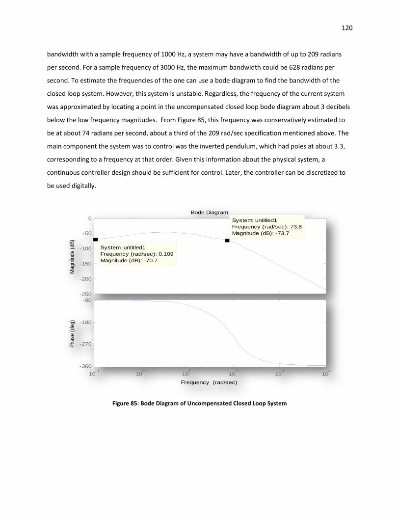
120
bandwidth with a sample frequency of 1000 Hz, a system may have a bandwidth of up to 209 radians
per second. For a sample frequency of 3000 Hz, the maximum bandwidth could be 628 radians per
second. To estimate the frequencies of the one can use a bode diagram to find the bandwidth of the
closed loop system. However, this system is unstable. Regardless, the frequency of the current system
was approximated by locating a point in the uncompensated closed loop bode diagram about 3 decibels
below the low frequency magnitudes. From Figure 85, this frequency was conservatively estimated to
be at about 74 radians per second, about a third of the 209 rad/sec specification mentioned above. The
main component the system was to control was the inverted pendulum, which had poles at about 3.3,
corresponding to a frequency at that order. Given this information about the physical system, a
continuous controller design should be sufficient for control. Later, the controller can be discretized to
be used digitally.
Figure 85: Bode Diagram of Uncompensated Closed Loop System
10-1
100
101
102
103
104
-360
-270
-180
-90
Pha
se (
deg)
Bode Diagram
Frequency (rad/sec)
-250
-200
-150
-100
-50
0
System: untitled1
Frequency (rad/sec): 0.109
Magnitude (dB): -70.7
Mag
nitu
de (
dB)
System: untitled1
Frequency (rad/sec): 73.8
Magnitude (dB): -73.7
121
6.2.4.3. PI Controller Design
Ultimately, a proportional integral (PI) controller was decided to be used to stabilize the system.
A PI controller introduces into the system a pole at the origin and a real zero away from the origin. The
pole at the origin was desirable for this system, because it would cancel the effect of the zero at the
origin contributed by the cylinder model. This way, the right hand plane branch may no longer terminate
at the origin, where all gains on the branch were in the right plane. However, at this point the system
was still unstable for any gains, because branches are formed off the real axis to the right of the
imaginary axis, as shown in Figure 86. In order to stabilize the system for some gain, these branches
must be moved into the left hand plane. This was the purpose of the zero in the PI controller. In order to
ensure poles could be selected away from the origin (slow response) and were in the left hand plane,
the zero must be greater in magnitude than the pole from the inverted pendulum. The diagram, then,
appears as shown in Figure 87 and Figure 88. At this level in the design, a wide range of combinations of
PI zero placement and gain selection exist to produce a stable system. Since the model used in the
controls analysis contained many assumptions and linear approximations, the root locus diagram, at this
level, acted more as a guide than a set of precise predictions. Additionally, the root locus diagram does
not account for saturation effects in the system. For example, the diagram may advise a gain that
requires 20 volt commands to the valve. However, the valve can only respond to 10 volts. As a result,
the simulation models described in section and subsections under 6.2.1.5: Simulink Models and Tools in
conjunction with exercising the actual system using LabVIEW, described in section and subsections
under 6.2.3: Data Acquisition and Control Tools, were used to vary the zero location and gain selection
and observe the system performance, namely the time required for the sled to drift out of the cylinder
stroke. The final selection was a real zero selection of seven and a gain selection of 1646, well below the
stable gain limit of about 2300. The root locus diagram and selection is shown in Figure 88. The resulting
system is expected to be underdamped with a frequency of about 40 Hz or 6.4 rad/sec . Figure 89 shows
the closed bode diagram of the compensated system. The bandwidth of the entire system was
approximately 66 rad/sec. For 30 times the frequency for sampling, a sample frequency of 316 Hz was
required, well below the 1000Hz target.
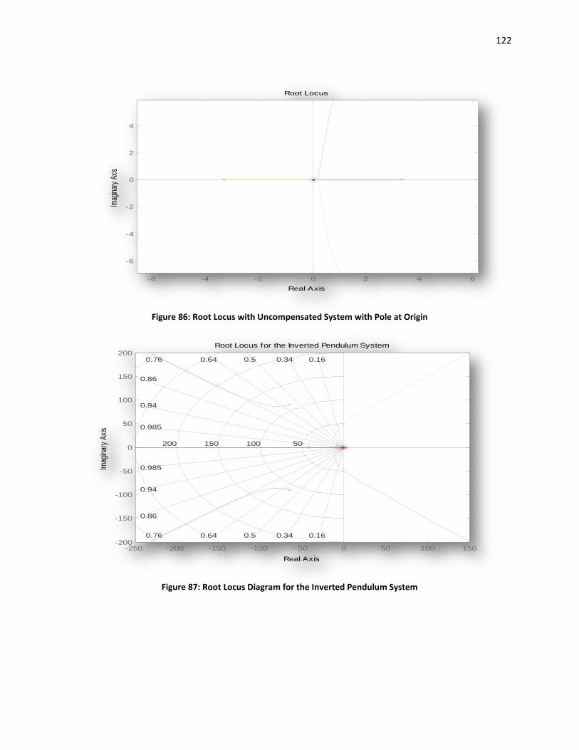
122
Figure 86: Root Locus with Uncompensated System with Pole at Origin
Figure 87: Root Locus Diagram for the Inverted Pendulum System
-6 -4 -2 0 2 4 6
-6
-4
-2
0
2
4
Root Locus
Real Axis
Imag
inar
y Ax
is
Root Locus for the Inverted Pendulum System
Real Axis
Imag
inar
y A
xis
-250 -200 -150 -100 -50 0 50 100 150-200
-150
-100
-50
0
50
100
150
2000.640.76
0.86
0.94
0.985
0.160.340.50.640.76
0.86
0.94
0.985
50100150200250
0.160.340.5
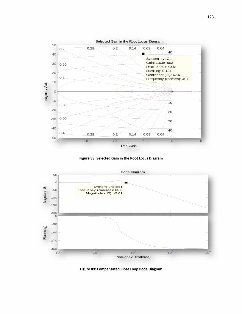
123
Figure 88: Selected Gain in the Root Locus Diagram
Figure 89: Compensated Close Loop Bode Diagram
Selected Gain in the Root Locus Diagram
Real Axis
Imag
inar
y A
xis
-20 -15 -10 -5 0 5-50
-40
-30
-20
-10
0
10
20
30
40
500.280.4
0.56
0.8
0.040.090.140.20.280.4
0.56
0.8
10
20
30
40
50
10
20
30
40
50
0.040.090.140.2
System: sysOL
Gain: 1.63e+003
Pole: -5.05 + 40.5i
Damping: 0.124
Overshoot (%): 67.6
Frequency (rad/sec): 40.8
100
101
102
103
104
-360
-270
-180
-90
0
Phas
e (d
eg)
Bode Diagram
Frequency (rad/sec)
-200
-150
-100
-50
0
50
Mag
nitu
de (d
B) System: untitled1
Frequency (rad/sec): 65.5
Magnitude (dB): -3.01
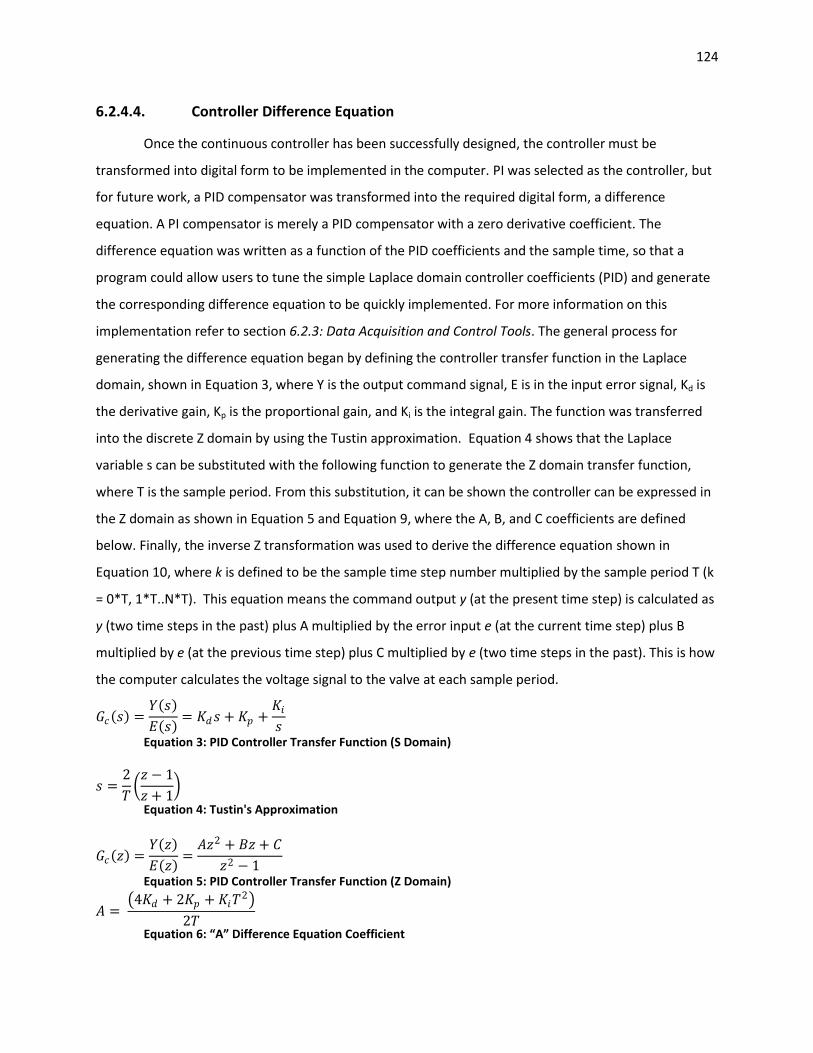
124
6.2.4.4. Controller Difference Equation
Once the continuous controller has been successfully designed, the controller must be
transformed into digital form to be implemented in the computer. PI was selected as the controller, but
for future work, a PID compensator was transformed into the required digital form, a difference
equation. A PI compensator is merely a PID compensator with a zero derivative coefficient. The
difference equation was written as a function of the PID coefficients and the sample time, so that a
program could allow users to tune the simple Laplace domain controller coefficients (PID) and generate
the corresponding difference equation to be quickly implemented. For more information on this
implementation refer to section 6.2.3: Data Acquisition and Control Tools. The general process for
generating the difference equation began by defining the controller transfer function in the Laplace
domain, shown in Equation 3, where Y is the output command signal, E is in the input error signal, Kd is
the derivative gain, Kp is the proportional gain, and Ki is the integral gain. The function was transferred
into the discrete Z domain by using the Tustin approximation. Equation 4 shows that the Laplace
variable s can be substituted with the following function to generate the Z domain transfer function,
where T is the sample period. From this substitution, it can be shown the controller can be expressed in
the Z domain as shown in Equation 5 and Equation 9, where the A, B, and C coefficients are defined
below. Finally, the inverse Z transformation was used to derive the difference equation shown in
Equation 10, where k is defined to be the sample time step number multiplied by the sample period T (k
= 0*T, 1*T..N*T). This equation means the command output y (at the present time step) is calculated as
y (two time steps in the past) plus A multiplied by the error input e (at the current time step) plus B
multiplied by e (at the previous time step) plus C multiplied by e (two time steps in the past). This is how
the computer calculates the voltage signal to the valve at each sample period.
𝐺𝑐 𝑠 =𝑌 𝑠
𝐸 𝑠 = 𝐾𝑑𝑠 + 𝐾𝑝 +
𝐾𝑖𝑠
Equation 3: PID Controller Transfer Function (S Domain)
𝑠 =2
𝑇 𝑧 − 1
𝑧 + 1
Equation 4: Tustin's Approximation
𝐺𝑐 𝑧 =𝑌 𝑧
𝐸 𝑧 =𝐴𝑧2 + 𝐵𝑧 + 𝐶
𝑧2 − 1
Equation 5: PID Controller Transfer Function (Z Domain)
𝐴 = 4𝐾𝑑 + 2𝐾𝑝 + 𝐾𝑖𝑇
2
2𝑇
Equation 6: “A” Difference Equation Coefficient
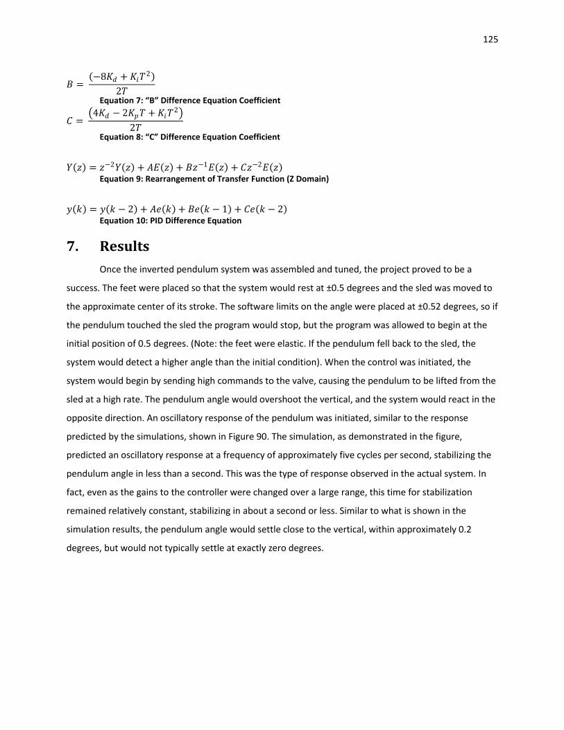
125
𝐵 = −8𝐾𝑑 + 𝐾𝑖𝑇
2
2𝑇
Equation 7: “B” Difference Equation Coefficient
𝐶 = 4𝐾𝑑 − 2𝐾𝑝𝑇 + 𝐾𝑖𝑇
2
2𝑇
Equation 8: “C” Difference Equation Coefficient
𝑌 𝑧 = 𝑧−2𝑌 𝑧 + 𝐴𝐸 𝑧 + 𝐵𝑧−1𝐸 𝑧 + 𝐶𝑧−2𝐸 𝑧 Equation 9: Rearrangement of Transfer Function (Z Domain)
𝑦 𝑘 = 𝑦 𝑘 − 2 + 𝐴𝑒 𝑘 + 𝐵𝑒 𝑘 − 1 + 𝐶𝑒 𝑘 − 2 Equation 10: PID Difference Equation
7. Results
Once the inverted pendulum system was assembled and tuned, the project proved to be a
success. The feet were placed so that the system would rest at ±0.5 degrees and the sled was moved to
the approximate center of its stroke. The software limits on the angle were placed at ±0.52 degrees, so if
the pendulum touched the sled the program would stop, but the program was allowed to begin at the
initial position of 0.5 degrees. (Note: the feet were elastic. If the pendulum fell back to the sled, the
system would detect a higher angle than the initial condition). When the control was initiated, the
system would begin by sending high commands to the valve, causing the pendulum to be lifted from the
sled at a high rate. The pendulum angle would overshoot the vertical, and the system would react in the
opposite direction. An oscillatory response of the pendulum was initiated, similar to the response
predicted by the simulations, shown in Figure 90. The simulation, as demonstrated in the figure,
predicted an oscillatory response at a frequency of approximately five cycles per second, stabilizing the
pendulum angle in less than a second. This was the type of response observed in the actual system. In
fact, even as the gains to the controller were changed over a large range, this time for stabilization
remained relatively constant, stabilizing in about a second or less. Similar to what is shown in the
simulation results, the pendulum angle would settle close to the vertical, within approximately 0.2
degrees, but would not typically settle at exactly zero degrees.
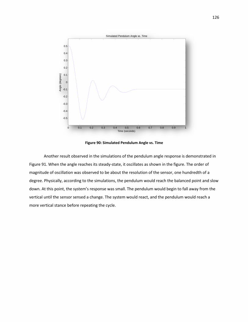
126
Figure 90: Simulated Pendulum Angle vs. Time
Another result observed in the simulations of the pendulum angle response is demonstrated in
Figure 91. When the angle reaches its steady-state, it oscillates as shown in the figure. The order of
magnitude of oscillation was observed to be about the resolution of the sensor, one hundredth of a
degree. Physically, according to the simulations, the pendulum would reach the balanced point and slow
down. At this point, the system’s response was small. The pendulum would begin to fall away from the
vertical until the sensor sensed a change. The system would react, and the pendulum would reach a
more vertical stance before repeating the cycle.
0 0.1 0.2 0.3 0.4 0.5 0.6 0.7 0.8 0.9 1
-0.5
-0.4
-0.3
-0.2
-0.1
0
0.1
0.2
0.3
0.4
0.5
Simulated Pendulum Angle vs. Time
Time (seconds)
Angle
(degre
es)
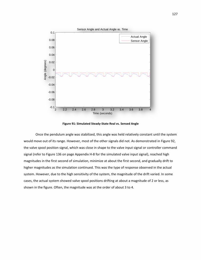
127
Figure 91: Simulated Steady-State Real vs. Sensed Angle
Once the pendulum angle was stabilized, this angle was held relatively constant until the system
would move out of its range. However, most of the other signals did not. As demonstrated in Figure 92,
the valve spool position signal, which was close in shape to the valve input signal or controller command
signal (refer to Figure 136 on page Appendix H-8 for the simulated valve input signal), reached high
magnitudes in the first second of simulation, minimize at about the first second, and gradually drift to
higher magnitudes as the simulation continued. This was the type of response observed in the actual
system. However, due to the high sensitivity of the system, the magnitude of the drift varied. In some
cases, the actual system showed valve spool positions drifting at about a magnitude of 2 or less, as
shown in the figure. Often, the magnitude was at the order of about 3 to 4.
2 2.2 2.4 2.6 2.8 3 3.2 3.4 3.6 3.8 4-0.1
-0.08
-0.06
-0.04
-0.02
0
0.02
0.04
0.06
0.08
0.1Sensor Angle and Actual Angle vs. Time
Time (seconds)
Angle
(degre
es)
Actual Angle
Sensor Angle
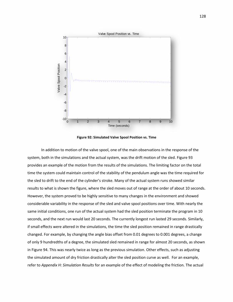
128
Figure 92: Simulated Valve Spool Position vs. Time
In addition to motion of the valve spool, one of the main observations in the response of the
system, both in the simulations and the actual system, was the drift motion of the sled. Figure 93
provides an example of the motion from the results of the simulations. The limiting factor on the total
time the system could maintain control of the stability of the pendulum angle was the time required for
the sled to drift to the end of the cylinder’s stroke. Many of the actual system runs showed similar
results to what is shown the figure, where the sled moves out of range at the order of about 10 seconds.
However, the system proved to be highly sensitive to many changes in the environment and showed
considerable variability in the response of the sled and valve spool positions over time. With nearly the
same initial conditions, one run of the actual system had the sled position terminate the program in 10
seconds, and the next run would last 20 seconds. The currently longest run lasted 29 seconds. Similarly,
if small effects were altered in the simulations, the time the sled position remained in range drastically
changed. For example, by changing the angle bias offset from 0.01 degrees to 0.001 degrees, a change
of only 9 hundredths of a degree, the simulated sled remained in range for almost 20 seconds, as shown
in Figure 94. This was nearly twice as long as the previous simulation. Other effects, such as adjusting
the simulated amount of dry friction drastically alter the sled position curve as well. For an example,
refer to Appendix H: Simulation Results for an example of the effect of modeling the friction. The actual
0 1 2 3 4 5 6 7 8 9 10-10
-8
-6
-4
-2
0
2
4
6
8
10Valve Spool Position vs. Time
Time (seconds)
Valv
e S
pool P
ositio
n
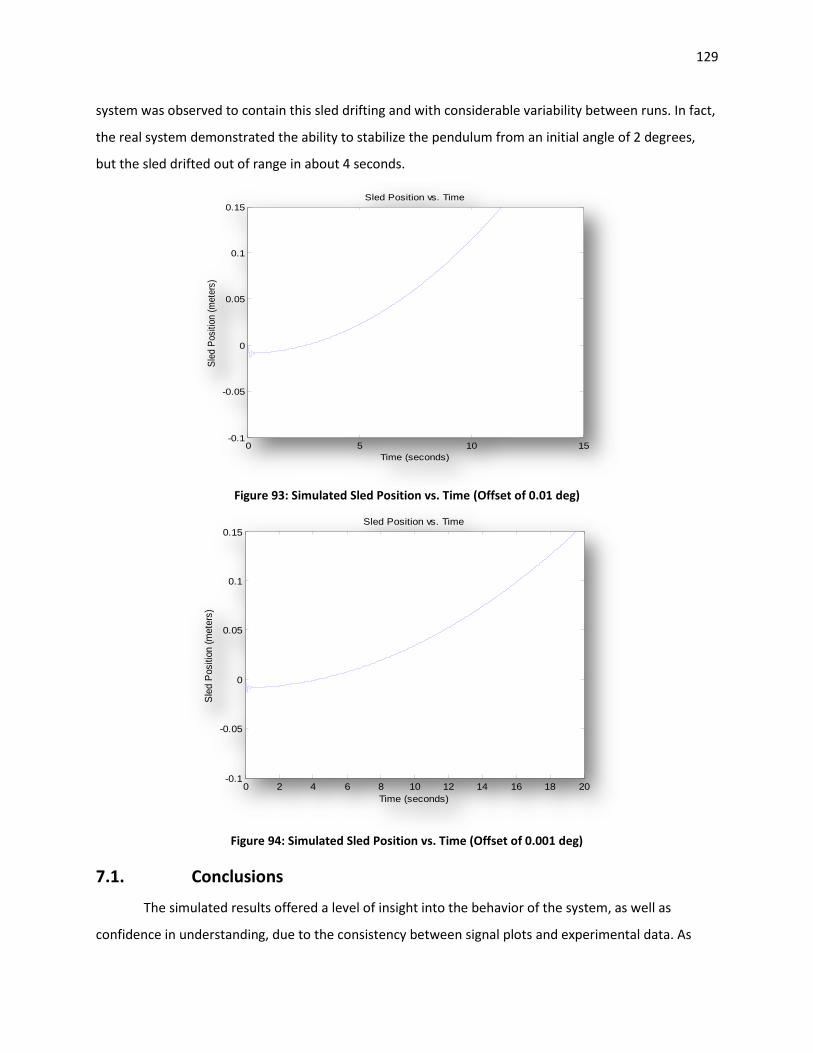
129
system was observed to contain this sled drifting and with considerable variability between runs. In fact,
the real system demonstrated the ability to stabilize the pendulum from an initial angle of 2 degrees,
but the sled drifted out of range in about 4 seconds.
Figure 93: Simulated Sled Position vs. Time (Offset of 0.01 deg)
Figure 94: Simulated Sled Position vs. Time (Offset of 0.001 deg)
7.1. Conclusions
The simulated results offered a level of insight into the behavior of the system, as well as
confidence in understanding, due to the consistency between signal plots and experimental data. As
0 5 10 15-0.1
-0.05
0
0.05
0.1
0.15Sled Position vs. Time
Time (seconds)
Sle
d P
ositi
on (
mete
rs)
0 2 4 6 8 10 12 14 16 18 20-0.1
-0.05
0
0.05
0.1
0.15Sled Position vs. Time
Time (seconds)
Sle
d P
ositio
n (
mete
rs)
130
shown in the root locus diagram in Figure 88 on page 123, the frequency of the system was expected to
be on the order of 5 cycles per second, the settling time was expected to be on the order of a second,
and the response was predicted to be under damped. All of these characteristics were both evident in
the simulated pendulum angle plots and the experimental results. Additionally, the diagram showed
that for a large range of gains, the frequency and settling time of the system should not vary
significantly. At a gain of 1200, the under damped poles were expected to generate a response at about
35 radians/sec or 5.6 Hz and a settling time on the order of 0.5 seconds. For a gain of 2000, the
frequency only increased by 5 radians/sec or 0.8 Hz, and the estimated settling time increased to 1.4
seconds. The actual system’s response to changes in gain value did not vary significantly either.
The simulated steady-state angle trend shown in Figure 91 on page 127 may provide a viable
reason for the drifting of the sled. The figure shows that when the angle stabilizes, it begins a cycle of
falling away from and rising towards the vertical at an amplitude of about a pulse from the angular
encoder, or one hundredth of a degree. The most likely reason for this is that the pendulum nearly
balanced at a point close to the vertical and began to fall back. This motion was undetected by the
system due to the resolution of the sensor. When the pendulum reached the next pulse, the system
reacted to the change in position, moving the pendulum back up to repeat the cycle. While the cycle
kept repeating, the system was adjusting the pendulum angle by moving the sled in one direction at
each cycle period. This may explain the slow drifting of the pendulum in a single direction.
Despite the similarities between the actual system and the simulated system, some
discrepancies existed. The inverted pendulum was balanced by the control system. The simulations were
useful for predicting trends within the response, as discussed in the Results section, but more precise
predictions of the signals proved difficult. For instance, the simulations might have predicted drift of the
valve voltage signal away from zero over time, as seen in the actual response, at a magnitude of about 2
volts, but the actual magnitude was observed to be at approximately 3 to 4 volts. The simulation
showed the system’s ability to stabilize the pendulum at lower proportional gains than the actual system
was capable of. The main reasons for these discrepancies were suspected to be due to physical
tolerances and nonlinearities in the valve and cylinder dynamics, not accounted for in the models.
Firstly, the existence of manufacturing tolerances and variability in the state of the physical
system was present. The main difficulty in setting up the system was the definition of the vertically
balanced position of the pendulum. To define this point, where the angular sensor sensed zero degrees
when the pendulum was balanced, the vertical alignment of the pendulum bar was insufficient. The
pendulum may not necessarily be balanced if one of its components is standing straight. Therefore, the
131
zero point had to be set within the software, not by aligning the physical components with the z-offset
position in the angular encoder. This value was approximated in the software by experiment. The
“home” position of the sensor was adjusted and the total control time for both the positive and negative
angle initial conditions were recorded over several runs. The times were averaged. The more centered
the “home” position was, the closer the positive and negative initial angle average run times should be.
However, after the vertical position was estimated, it would change the next time the bench holding the
system was moved. As a result, an offset in the sensed angle was present, difficult to quantify, and
changing over time. This would account for differences in the simulation and the real system.
Additionally, tolerances in the alignment of the pivot shaft in the pendulum joint were observed
during the experiments. This contributed to friction in the joint. However, this also may have been
changing with time. More stiction was observed in the joint at times than what was observed at other
times. The simulations demonstrated that friction played a major role in the sled response.
Secondly, the valve and cylinder were modeled to be linear. However, the coefficients in the
transfer functions were known to change for different command voltages, an indication of nonlinearity.
The coefficients were selected from the 5 volt command data, although the command voltages
observed during an actual control run was constantly changing. As a result, the simulations were using
slightly but sufficiently different representations of the dynamics of these components. Furthermore, a
constant command was used in the system identification process. A varying command was used in the
actual system. These differences may explain the main differences between the theoretical and actual
results.
Another nonlinearity not considered in the model but observed in the real system was the
cushions present in the hydraulic cylinder. Pressurized fluid is used at the ends of the cylinder to cushion
of the motion of the rod near the ends of its stroke. The dynamics of the cylinder in these regions are
considerable different than the main region of the component. As a result, often the sled would drift
until it reached this point, experience a change in velocity due to the cushion, causing the pendulum to
shift to the other side of the vertical, and begin to drift in the opposite direction. The simulations, on the
other hand, would predict the sled to simply drift out of range and stop.
7.2. Lessons Learned
Manufacturing tolerances in comparison to theoretical modeling
o The theoretical modeling of the system takes into account a completely frictionless
pivot joint. However, with the manufacturing tolerances witnessed as well as the slight
132
misalignment, it was apparent that the system induced external friction. A perfect real
world system is next to impossible.
Stack-ups
o Stack-ups are crucial when converging machined components into a physical system.
Each machined component has a tolerance that can negatively or positively affect its
relationship to a mating or adjacent part. In this project, stack-ups were pivotal when
defining the specifications for components of the system, as well as maintaining
continuity and alignment within the assembly.
Machining
o Machining operations as well as the machine itself can make or break a physical system.
The machining operations administered were achieved mainly on a 3-axis mill with
digital read outs and a standard lathe. Human error is the most frequent source of error
when a component is not properly machined.
Supplier/engineer relations
o Effective communication is pivotal to ensuring the exact components specified arrive as
desired. Misumi-USA has taken strides forward in configurable parts. Their online
interactive website allows for an easy to understand parts schematic and catalog setup.
They also offer 3D interactive modeling to see the part prior to quoting or purchasing.
Misumi-USA has proven to be an excellent source for ordering custom configurable
machined components.
Software Component Design
o To ensure software tools work as expected, minimizing errors, tools need to broken into
individual components and properly tested. This makes the whole project more
manageable and easier to debug, as the testing for errors is isolated to only individual
components.
Simulation Design
o As in software in general, testing individual components is important. One of the major
advantages to using software like Simulink is that each individual signal between blocks
can be plotted. In this way, the designer can verify each block and component is
behaving as expected before making conclusions about the systems as a whole. For
133
instance, the sensor quantization in the program could be easily verified by using a
“scope” block in the diagram.
Analytical Modeling
o Models should begin simple, using assumptions and approximations, and complicating
effects should be gradually and individually introduced to the model over time. The
advantage to this approach is that the simple model can provide general trends and
relationships. This can provide important insight for the designer on how the system
changes as different parameters are varied. Introducing other effects individually helps
show their individual contributions. This approach, in general, allows the engineer to
understand the system better than simply modeling everything from the beginning. For
example, the pendulum could be first modeled as a single bar. This way, the length and
weight of the bar and their effects on the system could be isolated. Later, the bar could
be modeled as a composite inertia, mass, and length to center of gravity.
System Identification
o To generate a reasonable representation of a system or subsystem to be used, an
appropriate excitation is important. In the project, step excitation was utilized to
characterize the model of the valve and cylinder. However, the command to the valve in
the inverted pendulum system is dynamic, both in the positive and negative regions in a
single control run. To best characterize any system, the conditions should be as close as
possible to what will actually be applied.
7.3. Recommendations
Control Sled Position
o By controlling the sled position within the control logic, the system could further control
the stability of the drift. The cylinder would not run out of stroke and the system could
fully stabilize itself.
Better Valve and Cylinder Model
o A step response was used at 5 Volts, maybe a square wave at smaller voltages could be
utilized for better command representation.
PID control, Phase lag, Phase lead-lag
o By examining other compensators, the system could respond much faster as well as a
much more consistent response.
134
Strings at end of stroke
o By utilizing a string on either end, the pendulum could physically hit the string to
continue the control of the system when the sled drifts and the cylinder runs out of
stroke.
Better initial conditions
o By integrating a release mechanism to the physical system, the pendulum could be
released at precisely zero degrees. This would allow for an initial velocity of zero as well.
On the other hand, the mechanism could also release the pendulum at an initial angle or
with an initial velocity.
Longer Pendulum
o A longer pendulum would slow the system down making it easier for the system to
respond to and people could see what’s going on better at the slower speeds.
Better Valve
o A higher frequency valve could provide a much quicker valve thus eliminating the small
time between interchange. A valve with less deadband would also be advantageous,
because the valve would then be able to more accurately switch direction thus respond
quicker.
Higher Pressures
o The system was not run higher than 500 psi. A higher pressure would allow the cylinder
to travel at a higher velocity thus increasing the overall response of the system.
Analog sensor
o The physical system was designed to accommodate an analog sensor. It would be
advantageous to conduct an in-depth comparison of the overall response of the system
between each sensor. Also, analyzing such factors as noise, accuracy, etc.
Angular velocity feedback
o An angular velocity feedback loop would allow the system to react much quicker to the
dynamics of the pendulum. Control of the system would be more accurate when the
rate of travel is know, furthermore acceleration as well.
Linear velocity feedback
o A linear velocity feedback would also be very beneficial to further control the sled. The
more control on all aspects of the physical system, the more accurate the response will
be.

135
Data Recording
o Recording the data as the system is attempting to stabilize would be extremely
beneficial as an analytical tool. Monitoring the exact output of the sensor, valve,
position etc, will directly allow the user to see exactly how the system is responding in a
graphical form.
8. Bibliography
http://images.google.com/imgres?imgurl=http://www-control.uni-
paderborn.de/giflab/seesaw%2Bpendulum.gif&imgrefurl=http://www-control.uni-
paderborn.de/rundgang.html&h=339&w=407&sz=73&hl=en&start=24&tbnid=rWfygPYPbonEYM:&tbnh=104&tbn
w=125&prev=/images%3Fq%3Dinverted%2Bpendulum%26start%3D18%26ndsp%3D18%26svnum%3D10%26hl%3
Den%26safe%3Dactive%26sa%3DN
http://images.google.com/imgres?imgurl=http://www.ecpsystems.com/subPageImages/penasscMain.gif
&imgrefurl=http://www.ecpsystems.com/controls_pendassc.htm&h=381&w=273&sz=27&hl=en&start=10&tbnid=
gGF8xdP2WJZ0xM:&tbnh=123&tbnw=88&prev=/images%3Fq%3Dinverted%2Bpendulum%26svnum%3D10%26hl%
3Den%26safe%3Dactive%26sa%3DN
http://images.google.com/imgres?imgurl=http://www.ece.osu.edu/~passino/4.jpg&imgrefurl=http://ww
w.ece.osu.edu/~passino/rip.html&h=426&w=279&sz=33&hl=en&start=6&tbnid=JU8JUnqWUdAEWM:&tbnh=126
&tbnw=83&prev=/images%3Fq%3Dinverted%2Bpendulum%26svnum%3D10%26hl%3Den%26safe%3Dactive%26sa
%3DN
http://images.google.com/imgres?imgurl=http://instruct1.cit.cornell.edu/courses/ee476/FinalProjects/s2
003/es89kh98/es89kh98/device_farview.JPG&imgrefurl=http://instruct1.cit.cornell.edu/courses/ee476/FinalProje
cts/s2003/es89kh98/es89kh98/index.htm&h=640&w=480&sz=59&hl=en&start=20&tbnid=FGRXmRukpAD_WM:&t
bnh=137&tbnw=103&prev=/images%3Fq%3Dinverted%2Bpendulum%26start%3D18%26ndsp%3D18%26svnum%3
D10%26hl%3Den%26safe%3Dactive%26sa%3DN
http://images.google.com/imgres?imgurl=http://www.control.toronto.edu/~bortoff/gifs/pend4.gif&imgrefurl=http://www.control.toronto.edu/~bortoff/pendulum.html&h=426&w=283&sz=168&hl=en&start=11&tbnid=U5JeeWqhdEgQAM:&tbnh=126&tbnw=84&prev=/images%3Fq%3Dinverted%2Bpendulum%26svnum%3D10%26hl%3Den%26safe%3Dactive%26sa%3DN

136
9. Acknowledgements
Thank you to Parker Hannifin Corporation for their generous contribution to fund this successful
endeavor.
Thank you to Dr. James Kamman for his genuine support, engineering knowledge, time, and
patience.
Thank you to Dr. Kapseong Ro for his time and encouragement.
Thank you to Glenn Hall for his expansive knowledge in machining and for his generous support.
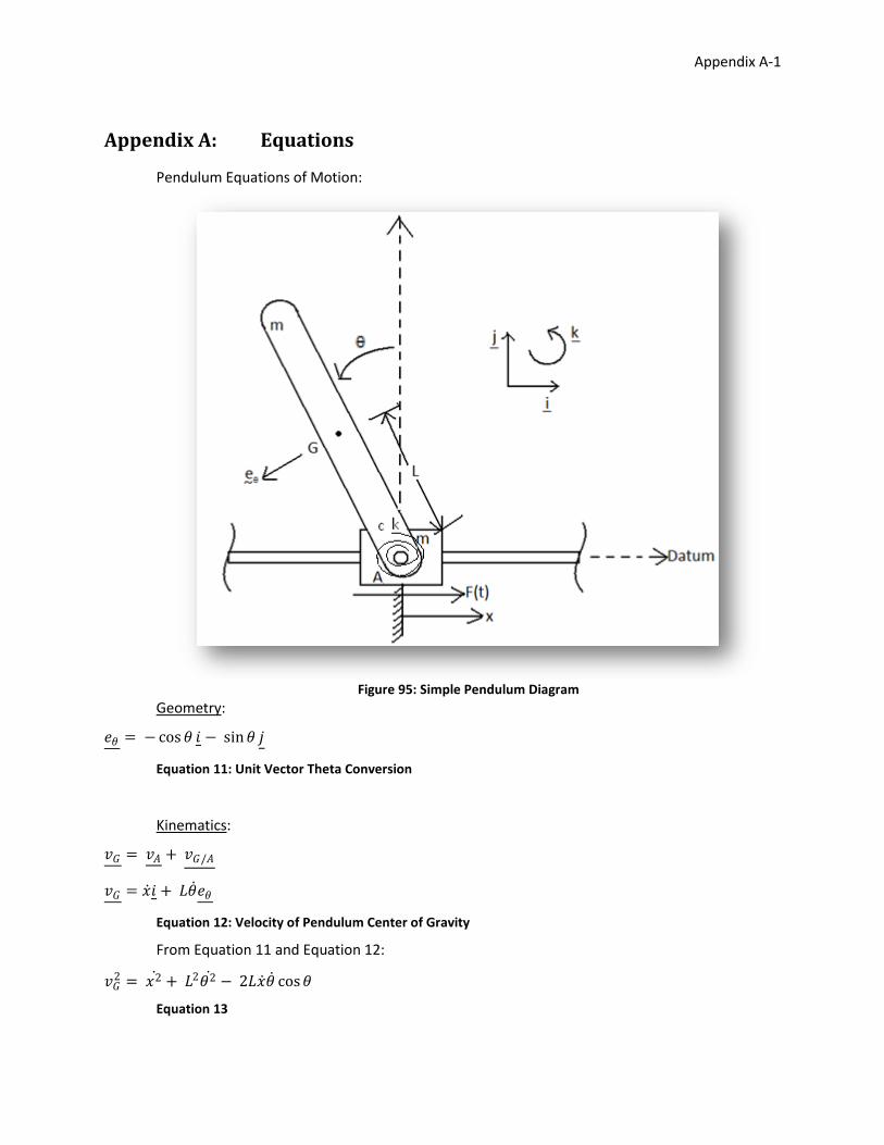
Appendix A-1
Appendix A: Equations
Pendulum Equations of Motion:
Figure 95: Simple Pendulum Diagram
Geometry:
𝑒𝜃 = − cos𝜃 𝑖 − sin𝜃 𝑗
Equation 11: Unit Vector Theta Conversion
Kinematics:
𝑣𝐺 = 𝑣𝐴 + 𝑣𝐺/𝐴
𝑣𝐺 = 𝑥 𝑖 + 𝐿𝜃 𝑒𝜃
Equation 12: Velocity of Pendulum Center of Gravity
From Equation 11 and Equation 12:
𝑣𝐺2 = 𝑥2 + 𝐿2𝜃2 − 2𝐿𝑥 𝜃 cos𝜃
Equation 13
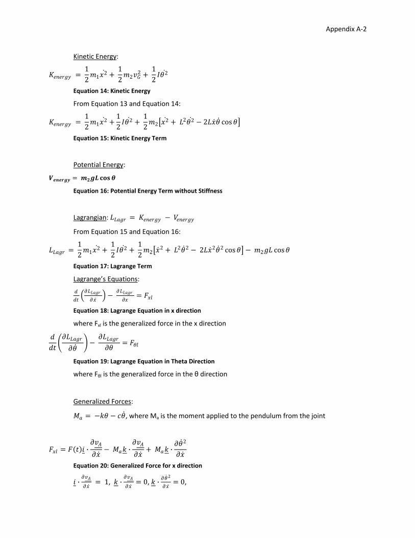
Appendix A-2
Kinetic Energy:
𝐾𝑒𝑛𝑒𝑟𝑔𝑦 = 1
2𝑚1𝑥
2 + 1
2𝑚2𝑣𝐺
2 + 1
2𝐼𝜃2
Equation 14: Kinetic Energy
From Equation 13 and Equation 14:
𝐾𝑒𝑛𝑒𝑟𝑔𝑦 = 1
2𝑚1𝑥
2 +1
2𝐼𝜃2 +
1
2𝑚2 𝑥
2 + 𝐿2𝜃2 − 2𝐿𝑥 𝜃 cos𝜃
Equation 15: Kinetic Energy Term
Potential Energy:
𝑽𝒆𝒏𝒆𝒓𝒈𝒚 = 𝒎𝟐𝒈𝑳𝐜𝐨𝐬 𝜽
Equation 16: Potential Energy Term without Stiffness
Lagrangian: 𝐿𝐿𝑎𝑔𝑟 = 𝐾𝑒𝑛𝑒𝑟𝑔𝑦 − 𝑉𝑒𝑛𝑒𝑟𝑔𝑦
From Equation 15 and Equation 16:
𝐿𝐿𝑎𝑔𝑟 = 1
2𝑚1𝑥
2 + 1
2𝐼𝜃2 +
1
2𝑚2 𝑥
2 + 𝐿2𝜃 2 − 2𝐿𝑥 2𝜃 2 cos𝜃 − 𝑚2𝑔𝐿 cos𝜃
Equation 17: Lagrange Term
Lagrange’s Equations:
𝑑
𝑑𝑡 𝜕𝐿𝐿𝑎𝑔𝑟
𝜕𝑥 −
𝜕𝐿𝐿𝑎𝑔𝑟
𝜕𝑥= 𝐹𝑥𝑙
Equation 18: Lagrange Equation in x direction
where Fxl is the generalized force in the x direction
𝑑
𝑑𝑡 𝜕𝐿𝐿𝑎𝑔𝑟
𝜕𝜃 −
𝜕𝐿𝐿𝑎𝑔𝑟
𝜕𝜃= 𝐹𝜃𝑙
Equation 19: Lagrange Equation in Theta Direction
where Fθl is the generalized force in the θ direction
Generalized Forces:
𝑀𝑎 = −𝑘𝜃 − 𝑐𝜃 , where Ma is the moment applied to the pendulum from the joint
𝐹𝑥𝑙 = 𝐹 𝑡 𝑖 ∙𝜕𝑣𝐴
𝜕𝑥 − 𝑀𝑎𝑘 ∙
𝜕𝑣𝐴
𝜕𝑥 + 𝑀𝑎𝑘 ∙
𝜕𝜃 2
𝜕𝑥
Equation 20: Generalized Force for x direction
𝑖 ∙𝜕𝑣𝐴
𝜕𝑥 = 1, 𝑘 ∙
𝜕𝑣𝐴
𝜕𝑥 = 0, 𝑘 ∙
𝜕𝜃 2
𝜕𝑥 = 0,
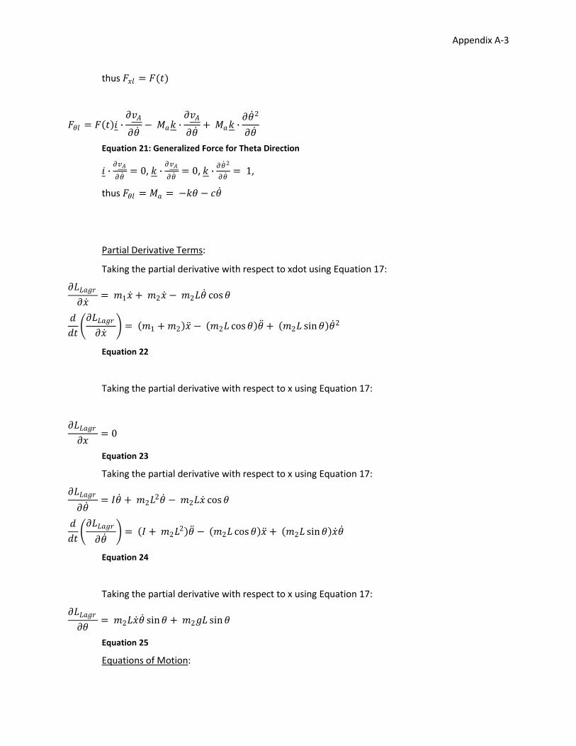
Appendix A-3
thus 𝐹𝑥𝑙 = 𝐹(𝑡)
𝐹𝜃𝑙 = 𝐹 𝑡 𝑖 ∙𝜕𝑣𝐴
𝜕𝜃 − 𝑀𝑎𝑘 ∙
𝜕𝑣𝐴
𝜕𝜃 + 𝑀𝑎𝑘 ∙
𝜕𝜃 2
𝜕𝜃
Equation 21: Generalized Force for Theta Direction
𝑖 ∙𝜕𝑣𝐴
𝜕𝜃 = 0, 𝑘 ∙
𝜕𝑣𝐴
𝜕𝜃 = 0, 𝑘 ∙
𝜕𝜃 2
𝜕𝜃 = 1,
thus 𝐹𝜃𝑙 = 𝑀𝑎 = −𝑘𝜃 − 𝑐𝜃
Partial Derivative Terms:
Taking the partial derivative with respect to xdot using Equation 17:
𝜕𝐿𝐿𝑎𝑔𝑟
𝜕𝑥 = 𝑚1𝑥 + 𝑚2𝑥 − 𝑚2𝐿𝜃 cos𝜃
𝑑
𝑑𝑡 𝜕𝐿𝐿𝑎𝑔𝑟
𝜕𝑥 = 𝑚1 + 𝑚2 𝑥 − 𝑚2𝐿 cos𝜃 𝜃 + 𝑚2𝐿 sin𝜃 𝜃 2
Equation 22
Taking the partial derivative with respect to x using Equation 17:
𝜕𝐿𝐿𝑎𝑔𝑟
𝜕𝑥= 0
Equation 23
Taking the partial derivative with respect to x using Equation 17:
𝜕𝐿𝐿𝑎𝑔𝑟
𝜕𝜃 = 𝐼𝜃 + 𝑚2𝐿
2𝜃 − 𝑚2𝐿𝑥 cos𝜃
𝑑
𝑑𝑡 𝜕𝐿𝐿𝑎𝑔𝑟
𝜕𝜃 = 𝐼 + 𝑚2𝐿
2 𝜃 − 𝑚2𝐿 cos𝜃 𝑥 + 𝑚2𝐿 sin𝜃 𝑥 𝜃
Equation 24
Taking the partial derivative with respect to x using Equation 17:
𝜕𝐿𝐿𝑎𝑔𝑟
𝜕𝜃= 𝑚2𝐿𝑥 𝜃 sin𝜃 + 𝑚2𝑔𝐿 sin𝜃
Equation 25
Equations of Motion:
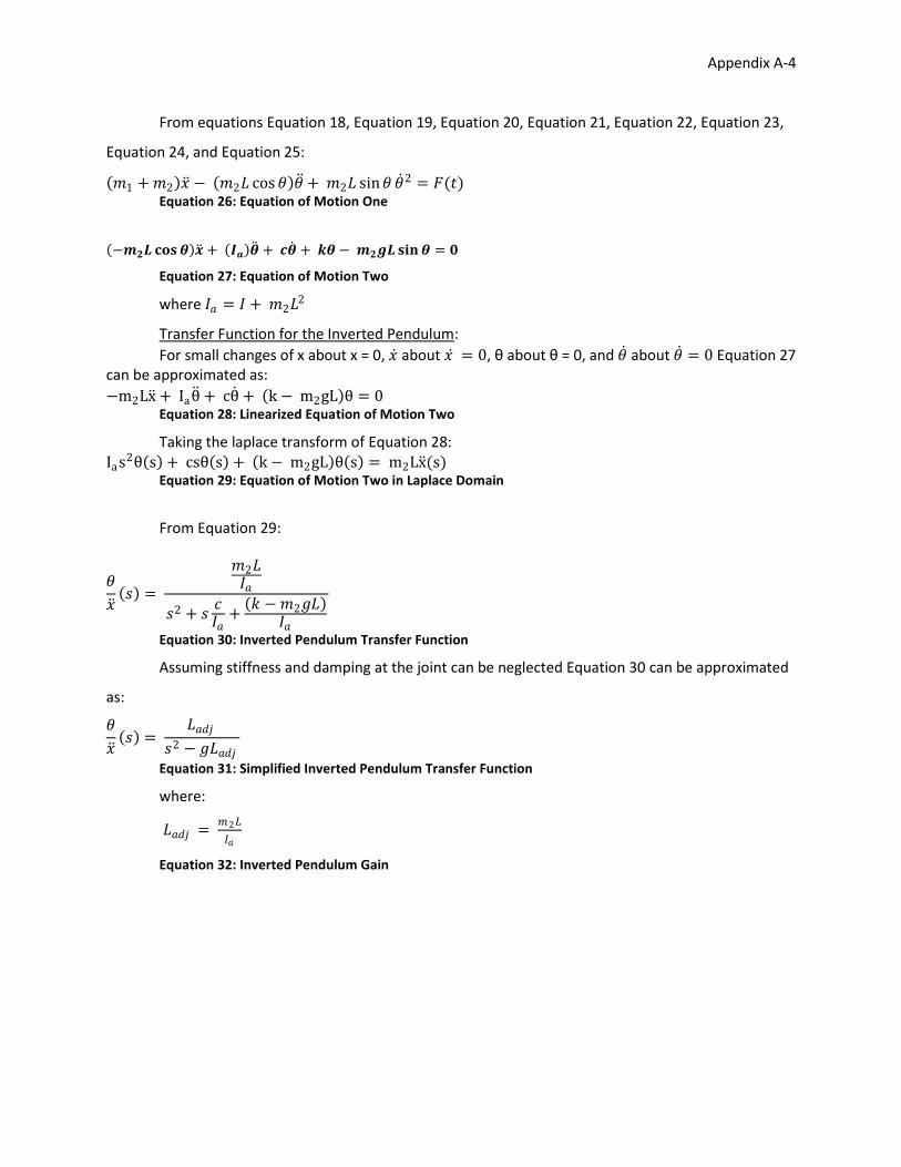
Appendix A-4
From equations Equation 18, Equation 19, Equation 20, Equation 21, Equation 22, Equation 23,
Equation 24, and Equation 25:
𝑚1 + 𝑚2 𝑥 − 𝑚2𝐿 cos𝜃 𝜃 + 𝑚2𝐿 sin𝜃 𝜃 2 = 𝐹(𝑡) Equation 26: Equation of Motion One
−𝒎𝟐𝑳 𝐜𝐨𝐬 𝜽 𝒙 + 𝑰𝒂 𝜽 + 𝒄𝜽 + 𝒌𝜽 − 𝒎𝟐𝒈𝑳𝐬𝐢𝐧 𝜽 = 𝟎
Equation 27: Equation of Motion Two
where 𝐼𝑎 = 𝐼 + 𝑚2𝐿2
Transfer Function for the Inverted Pendulum:
For small changes of x about x = 0, 𝑥 about 𝑥 = 0, θ about θ = 0, and 𝜃 about 𝜃 = 0 Equation 27 can be approximated as:
−m2Lx + Iaθ + cθ + k − m2gL θ = 0 Equation 28: Linearized Equation of Motion Two
Taking the laplace transform of Equation 28: Ias2θ s + csθ s + k − m2gL θ s = m2Lx (s)
Equation 29: Equation of Motion Two in Laplace Domain
From Equation 29:
𝜃
𝑥 𝑠 =
𝑚2𝐿𝐼𝑎
𝑠2 + 𝑠𝑐𝐼𝑎
+ 𝑘 − 𝑚2𝑔𝐿
𝐼𝑎
Equation 30: Inverted Pendulum Transfer Function
Assuming stiffness and damping at the joint can be neglected Equation 30 can be approximated
as:
𝜃
𝑥 𝑠 =
𝐿𝑎𝑑𝑗
𝑠2 − 𝑔𝐿𝑎𝑑𝑗
Equation 31: Simplified Inverted Pendulum Transfer Function
where:
𝐿𝑎𝑑𝑗 = 𝑚2𝐿
𝐼𝑎
Equation 32: Inverted Pendulum Gain
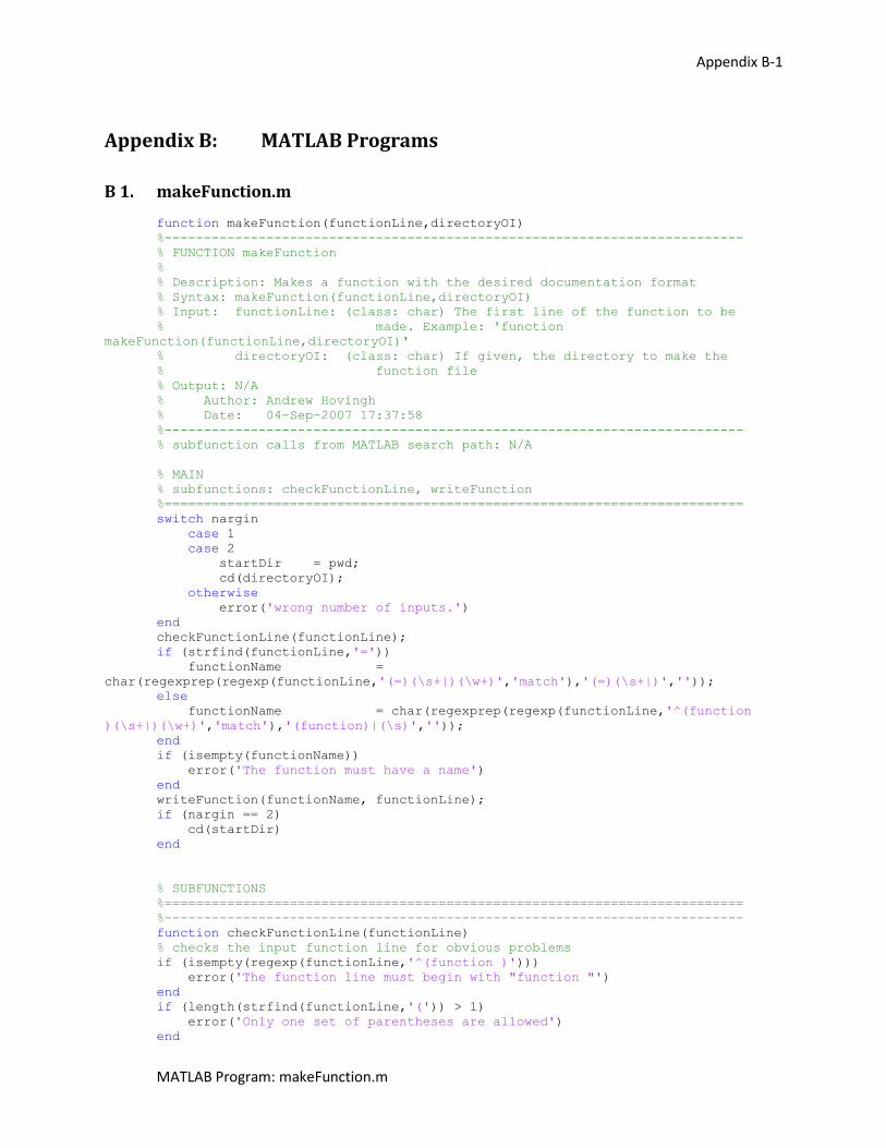
Appendix B-1
MATLAB Program: makeFunction.m
Appendix B: MATLAB Programs
B 1. makeFunction.m
function makeFunction(functionLine,directoryOI)
%--------------------------------------------------------------------------
% FUNCTION makeFunction
%
% Description: Makes a function with the desired documentation format
% Syntax: makeFunction(functionLine,directoryOI)
% Input: functionLine: (class: char) The first line of the function to be
% made. Example: 'function
makeFunction(functionLine,directoryOI)'
% directoryOI: (class: char) If given, the directory to make the
% function file
% Output: N/A
% Author: Andrew Hovingh
% Date: 04-Sep-2007 17:37:58
%--------------------------------------------------------------------------
% subfunction calls from MATLAB search path: N/A
% MAIN
% subfunctions: checkFunctionLine, writeFunction
%==========================================================================
switch nargin
case 1
case 2
startDir = pwd;
cd(directoryOI);
otherwise
error('wrong number of inputs.')
end
checkFunctionLine(functionLine);
if (strfind(functionLine,'='))
functionName =
char(regexprep(regexp(functionLine,'(=)(\s+|)(\w+)','match'),'(=)(\s+|)',''));
else
functionName = char(regexprep(regexp(functionLine,'^(function
)(\s+|)(\w+)','match'),'(function)|(\s)',''));
end
if (isempty(functionName))
error('The function must have a name')
end
writeFunction(functionName, functionLine);
if (nargin == 2)
cd(startDir)
end
% SUBFUNCTIONS
%==========================================================================
%--------------------------------------------------------------------------
function checkFunctionLine(functionLine)
% checks the input function line for obvious problems
if (isempty(regexp(functionLine,'^(function )')))
error('The function line must begin with "function "')
end
if (length(strfind(functionLine,'(')) > 1)
error('Only one set of parentheses are allowed')
end
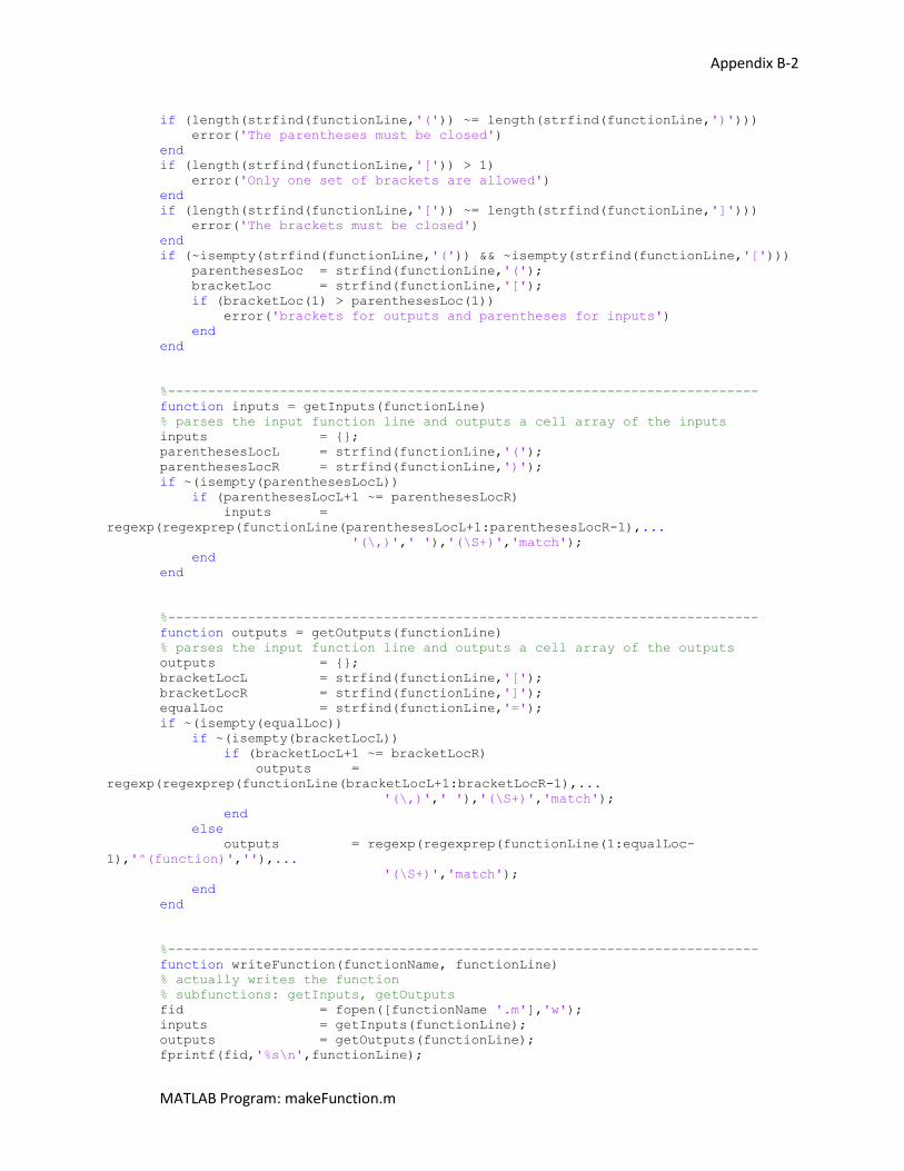
Appendix B-2
MATLAB Program: makeFunction.m
if (length(strfind(functionLine,'(')) ~= length(strfind(functionLine,')')))
error('The parentheses must be closed')
end
if (length(strfind(functionLine,'[')) > 1)
error('Only one set of brackets are allowed')
end
if (length(strfind(functionLine,'[')) ~= length(strfind(functionLine,']')))
error('The brackets must be closed')
end
if (~isempty(strfind(functionLine,'(')) && ~isempty(strfind(functionLine,'[')))
parenthesesLoc = strfind(functionLine,'(');
bracketLoc = strfind(functionLine,'[');
if (bracketLoc(1) > parenthesesLoc(1))
error('brackets for outputs and parentheses for inputs')
end
end
%--------------------------------------------------------------------------
function inputs = getInputs(functionLine)
% parses the input function line and outputs a cell array of the inputs
inputs = {};
parenthesesLocL = strfind(functionLine,'(');
parenthesesLocR = strfind(functionLine,')');
if ~(isempty(parenthesesLocL))
if (parenthesesLocL+1 ~= parenthesesLocR)
inputs =
regexp(regexprep(functionLine(parenthesesLocL+1:parenthesesLocR-1),...
'(\,)',' '),'(\S+)','match');
end
end
%--------------------------------------------------------------------------
function outputs = getOutputs(functionLine)
% parses the input function line and outputs a cell array of the outputs
outputs = {};
bracketLocL = strfind(functionLine,'[');
bracketLocR = strfind(functionLine,']');
equalLoc = strfind(functionLine,'=');
if ~(isempty(equalLoc))
if ~(isempty(bracketLocL))
if (bracketLocL+1 ~= bracketLocR)
outputs =
regexp(regexprep(functionLine(bracketLocL+1:bracketLocR-1),...
'(\,)',' '),'(\S+)','match');
end
else
outputs = regexp(regexprep(functionLine(1:equalLoc-
1),'^(function)',''),...
'(\S+)','match');
end
end
%--------------------------------------------------------------------------
function writeFunction(functionName, functionLine)
% actually writes the function
% subfunctions: getInputs, getOutputs
fid = fopen([functionName '.m'],'w');
inputs = getInputs(functionLine);
outputs = getOutputs(functionLine);
fprintf(fid,'%s\n',functionLine);
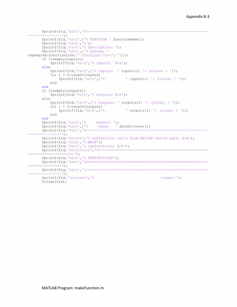
Appendix B-3
MATLAB Program: makeFunction.m
fprintf(fid,'%s\n','%----------------------------------------------------------
----------------');
fprintf(fid,'%s\n',['% FUNCTION ' functionName]);
fprintf(fid,'%s\n','%');
fprintf(fid,'%s\n','% Description: ');
fprintf(fid,'%s\n',['% Syntax: '
regexprep(functionLine,'^(function)(\s+)','')]);
if (isempty(inputs))
fprintf(fid,'%s\n','% Inputs: N/A');
else
fprintf(fid,'%s\n',['% Inputs: ' inputs{1} ': (class: ) ']);
for i = 2:length(inputs)
fprintf(fid,'%s\n',['% ' inputs{i} ': (class: ) ']);
end
end
if (isempty(outputs))
fprintf(fid,'%s\n','% Outputs: N/A');
else
fprintf(fid,'%s\n',['% Outputs: ' outputs{1} ': (class: ) ']);
for i = 2:length(outputs)
fprintf(fid,'%s\n',['% ' outputs{i} ': (class: ) ']);
end
end
fprintf(fid,'%s\n','% Author: ');
fprintf(fid,'%s\n',['% Date: ' datestr(now)]);
fprintf(fid,'%s\n','%----------------------------------------------------------
----------------');
fprintf(fid,'%s\n\n','% subfunction calls from MATLAB search path: N/A');
fprintf(fid,'%s\n','% MAIN');
fprintf(fid,'%s\n','% subfunctions: N/A');
fprintf(fid,'%s\n\n\n\n','%====================================================
======================');
fprintf(fid,'%s\n','% SUBFUNCTIONS');
fprintf(fid,'%s\n','%==========================================================
================');
fprintf(fid,'%s\n','%----------------------------------------------------------
----------------');
fprintf(fid,'%s\n\n\n','% --none--');
fclose(fid);
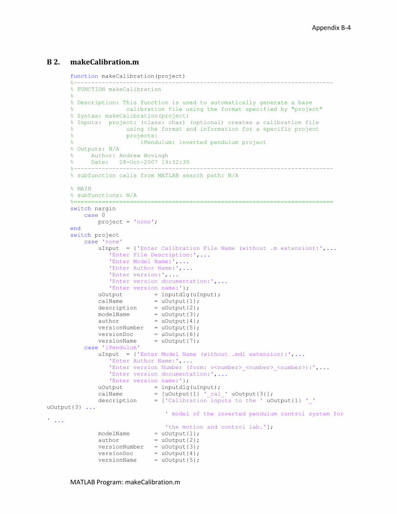
Appendix B-4
MATLAB Program: makeCalibration.m
B 2. makeCalibration.m
function makeCalibration(project)
%--------------------------------------------------------------------------
% FUNCTION makeCalibration
%
% Description: This function is used to automatically generate a base
% calibration file using the format specified by "project"
% Syntax: makeCalibration(project)
% Inputs: project: (class: char) (optional) creates a calibration file
% using the format and information for a specific project
% projects:
% iPendulum: inverted pendulum project
% Outputs: N/A
% Author: Andrew Hovingh
% Date: 28-Oct-2007 19:32:35
%--------------------------------------------------------------------------
% subfunction calls from MATLAB search path: N/A
% MAIN
% subfunctions: N/A
%==========================================================================
switch nargin
case 0
project = 'none';
end
switch project
case 'none'
uInput = {'Enter Calibration File Name (without .m extension):',...
'Enter File Description:',...
'Enter Model Name:',...
'Enter Author Name:',...
'Enter version:',...
'Enter version documentation:',...
'Enter version name:'};
uOutput = inputdlg(uInput);
calName = uOutput{1};
description = uOutput{2};
modelName = uOutput{3};
author = uOutput{4};
versionNumber = uOutput{5};
versionDoc = uOutput{6};
versionName = uOutput{7};
case 'iPendulum'
uInput = {'Enter Model Name (without .mdl extension):',...
'Enter Author Name:',...
'Enter version Number (form: v<number>_<number>_<number>):',...
'Enter version documentation:',...
'Enter version name:'};
uOutput = inputdlg(uInput);
calName = [uOutput{1} '_cal_' uOutput{3}];
description = ['Calibration inputs to the ' uOutput{1} '_'
uOutput{3} ...
' model of the inverted pendulum control system for
' ...
'the motion and control lab.'];
modelName = uOutput{1};
author = uOutput{2};
versionNumber = uOutput{3};
versionDoc = uOutput{4};
versionName = uOutput{5};
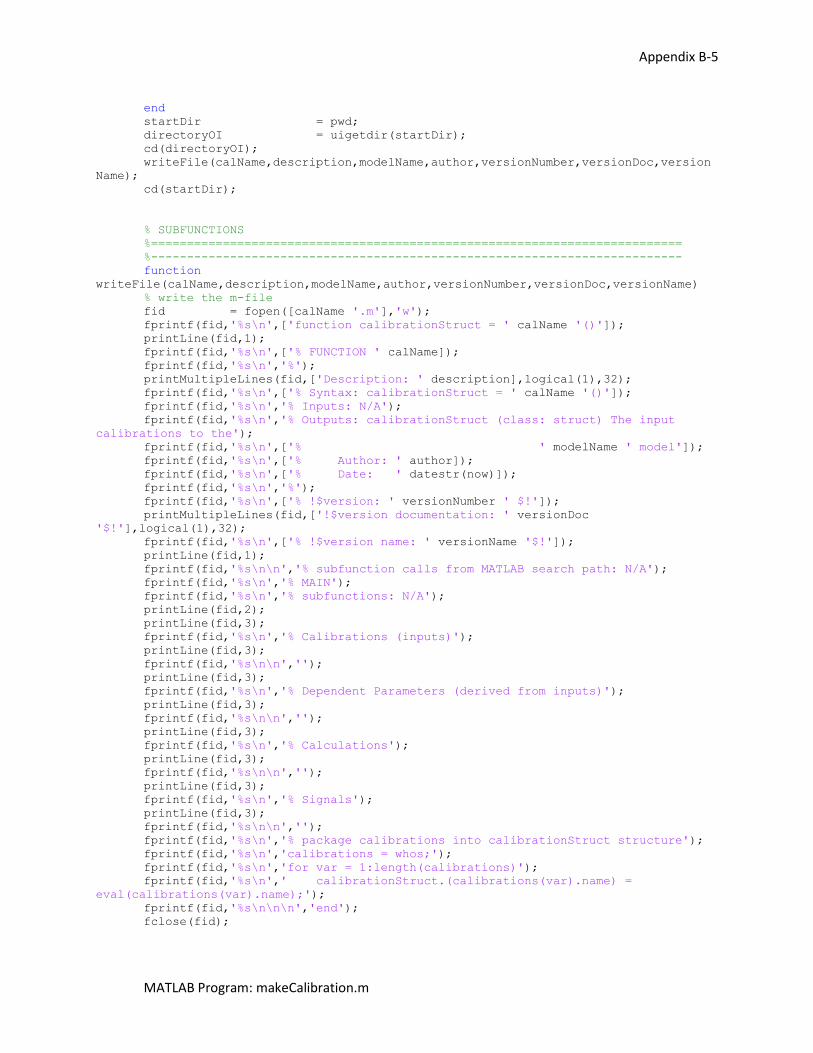
Appendix B-5
MATLAB Program: makeCalibration.m
end
startDir = pwd;
directoryOI = uigetdir(startDir);
cd(directoryOI);
writeFile(calName,description,modelName,author,versionNumber,versionDoc,version
Name);
cd(startDir);
% SUBFUNCTIONS
%==========================================================================
%--------------------------------------------------------------------------
function
writeFile(calName,description,modelName,author,versionNumber,versionDoc,versionName)
% write the m-file
fid = fopen([calName '.m'],'w');
fprintf(fid,'%s\n',['function calibrationStruct = ' calName '()']);
printLine(fid,1);
fprintf(fid,'%s\n',['% FUNCTION ' calName]);
fprintf(fid,'%s\n','%');
printMultipleLines(fid,['Description: ' description],logical(1),32);
fprintf(fid,'%s\n',['% Syntax: calibrationStruct = ' calName '()']);
fprintf(fid,'%s\n','% Inputs: N/A');
fprintf(fid,'%s\n','% Outputs: calibrationStruct (class: struct) The input
calibrations to the');
fprintf(fid,'%s\n',['% ' modelName ' model']);
fprintf(fid,'%s\n',['% Author: ' author]);
fprintf(fid,'%s\n',['% Date: ' datestr(now)]);
fprintf(fid,'%s\n','%');
fprintf(fid,'%s\n',['% !$version: ' versionNumber ' $!']);
printMultipleLines(fid,['!$version documentation: ' versionDoc
'$!'],logical(1),32);
fprintf(fid,'%s\n',['% !$version name: ' versionName '$!']);
printLine(fid,1);
fprintf(fid,'%s\n\n','% subfunction calls from MATLAB search path: N/A');
fprintf(fid,'%s\n','% MAIN');
fprintf(fid,'%s\n','% subfunctions: N/A');
printLine(fid,2);
printLine(fid,3);
fprintf(fid,'%s\n','% Calibrations (inputs)');
printLine(fid,3);
fprintf(fid,'%s\n\n','');
printLine(fid,3);
fprintf(fid,'%s\n','% Dependent Parameters (derived from inputs)');
printLine(fid,3);
fprintf(fid,'%s\n\n','');
printLine(fid,3);
fprintf(fid,'%s\n','% Calculations');
printLine(fid,3);
fprintf(fid,'%s\n\n','');
printLine(fid,3);
fprintf(fid,'%s\n','% Signals');
printLine(fid,3);
fprintf(fid,'%s\n\n','');
fprintf(fid,'%s\n','% package calibrations into calibrationStruct structure');
fprintf(fid,'%s\n','calibrations = whos;');
fprintf(fid,'%s\n','for var = 1:length(calibrations)');
fprintf(fid,'%s\n',' calibrationStruct.(calibrations(var).name) =
eval(calibrations(var).name);');
fprintf(fid,'%s\n\n\n','end');
fclose(fid);
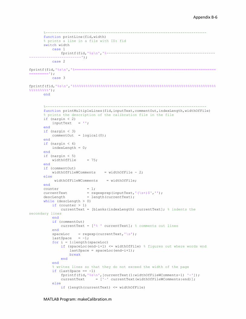
Appendix B-6
MATLAB Program: makeCalibration.m
%--------------------------------------------------------------------------
function printLine(fid,width)
% prints a line in a file with ID: fid
switch width
case 1
fprintf(fid,'%s\n','%--------------------------------------------------
------------------------');
case 2
fprintf(fid,'%s\n','%=================================================================
=========');
case 3
fprintf(fid,'%s\n','%%%%%%%%%%%%%%%%%%%%%%%%%%%%%%%%%%%%%%%%%%%%%%%%%%%%%%%%%%%%%%%%%%
%%%%%%%%%');
end
%--------------------------------------------------------------------------
function printMultipleLines(fid,inputText,commentOut,indexLength,widthOfFile)
% prints the description of the calibration file in the file
if (nargin < 2)
inputText = '';
end
if (nargin < 3)
commentOut = logical(0);
end
if (nargin < 4)
indexLength = 0;
end
if (nargin < 5)
widthOfFile = 75;
end
if (commentOut)
widthOfFileWComments = widthOfFile - 2;
else
widthOfFileWComments = widthOfFile;
end
counter = 1;
currentText = regexprep(inputText,'(\s+)$','');
descLength = length(currentText);
while (descLength > 0)
if (counter > 1)
currentText = [blanks(indexLength) currentText]; % indents the
secondary lines
end
if (commentOut)
currentText = ['% ' currentText]; % comments out lines
end
spaceLoc = regexp(currentText,'\s');
lastSpace = -1;
for i = 1:length(spaceLoc)
if (spaceLoc(end-i+1) <= widthOfFile) % figures out where words end
lastSpace = spaceLoc(end-i+1);
break
end
end
% writes lines so that they do not exceed the width of the page
if (lastSpace == -1)
fprintf(fid,'%s\n',[currentText(1:widthOfFileWComments-1) '-']);
currentText = ['-' currentText(widthOfFileWComments:end)];
else
if (length(currentText) <= widthOfFile)
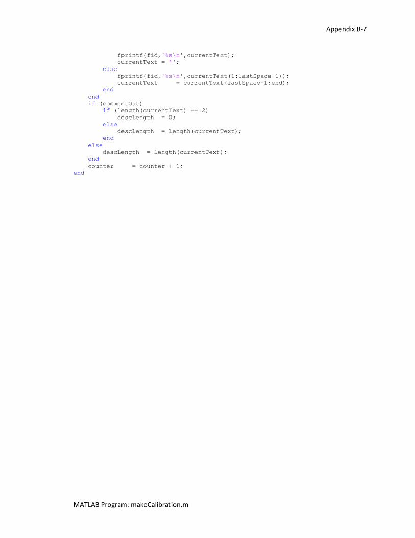
Appendix B-7
MATLAB Program: makeCalibration.m
fprintf(fid,'%s\n',currentText);
currentText = '';
else
fprintf(fid,'%s\n',currentText(1:lastSpace-1));
currentText = currentText(lastSpace+1:end);
end
end
if (commentOut)
if (length(currentText) == 2)
descLength = 0;
else
descLength = length(currentText);
end
else
descLength = length(currentText);
end
counter = counter + 1;
end
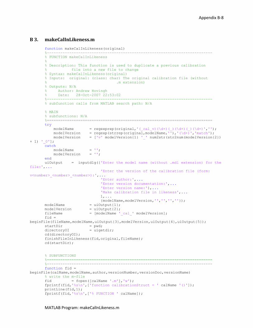
Appendix B-8
MATLAB Program: makeCalInLikeness.m
B 3. makeCalInLikeness.m
function makeCalInLikeness(original)
%--------------------------------------------------------------------------
% FUNCTION makeCalInLikeness
%
% Description: This function is used to duplicate a previous calibration
% file into a new file to change
% Syntax: makeCalInLikeness(original)
% Inputs: original: (class: char) The original calibration file (without
% .m extension)
% Outputs: N/A
% Author: Andrew Hovingh
% Date: 28-Oct-2007 22:53:02
%--------------------------------------------------------------------------
% subfunction calls from MATLAB search path: N/A
% MAIN
% subfunctions: N/A
%==========================================================================
try
modelName = regexprep(original,'(_cal_v)(\d+)(_)(\d+)(_)(\d+)','');
modelVersion = regexp(strrep(original,modelName,''),'(\d+)','match');
modelVersion = ['v' modelVersion{1} '_' num2str(str2num(modelVersion{2})
+ 1) '_0'];
catch
modelName = '';
modelVersion = '';
end
uiOutput = inputdlg({'Enter the model name (without .mdl extension) for the
file:',...
'Enter the version of the calibration file (form:
v<number>_<number>_<number>):',...
'Enter author:',...
'Enter version documentation:',...
'Enter version name:'},...
'Make calibration file in likeness',...
1,...
{modelName,modelVersion,'','','',''});
modelName = uiOutput{1};
modelVersion = uiOutput{2};
fileName = [modelName '_cal_' modelVersion];
fid =
beginFile(fileName,modelName,uiOutput{3},modelVersion,uiOutput{4},uiOutput{5});
startDir = pwd;
directoryOI = uigetdir;
cd(directoryOI);
finishFileInLikeness(fid,original,fileName);
cd(startDir);
% SUBFUNCTIONS
%==========================================================================
%--------------------------------------------------------------------------
function fid =
beginFile(calName,modelName,author,versionNumber,versionDoc,versionName)
% write the m-file
fid = fopen([calName '.m'],'w');
fprintf(fid,'%s\n',['function calibrationStruct = ' calName '()']);
printLine(fid,1);
fprintf(fid,'%s\n',['% FUNCTION ' calName]);
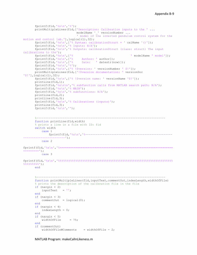
Appendix B-9
MATLAB Program: makeCalInLikeness.m
fprintf(fid,'%s\n','%');
printMultipleLines(fid,['Description: Calibration inputs to the ' ...
modelName '_' versionNumber ...
' model of the inverted pendulum control system for the
motion and control lab.'],logical(1),32);
fprintf(fid,'%s\n',['% Syntax: calibrationStruct = ' calName '()']);
fprintf(fid,'%s\n','% Inputs: N/A');
fprintf(fid,'%s\n','% Outputs: calibrationStruct (class: struct) The input
calibrations to the');
fprintf(fid,'%s\n',['% ' modelName ' model']);
fprintf(fid,'%s\n',['% Author: ' author]);
fprintf(fid,'%s\n',['% Date: ' datestr(now)]);
fprintf(fid,'%s\n','%');
fprintf(fid,'%s\n',['% !$version: ' versionNumber ' $!']);
printMultipleLines(fid,['!$version documentation: ' versionDoc
'$!'],logical(1),32);
fprintf(fid,'%s\n',['% !$version name: ' versionName '$!']);
printLine(fid,1);
fprintf(fid,'%s\n\n','% subfunction calls from MATLAB search path: N/A');
fprintf(fid,'%s\n','% MAIN');
fprintf(fid,'%s\n','% subfunctions: N/A');
printLine(fid,2);
printLine(fid,3);
fprintf(fid,'%s\n','% Calibrations (inputs)');
printLine(fid,3);
fprintf(fid,'%s\n','');
%--------------------------------------------------------------------------
function printLine(fid,width)
% prints a line in a file with ID: fid
switch width
case 1
fprintf(fid,'%s\n','%--------------------------------------------------
------------------------');
case 2
fprintf(fid,'%s\n','%=================================================================
=========');
case 3
fprintf(fid,'%s\n','%%%%%%%%%%%%%%%%%%%%%%%%%%%%%%%%%%%%%%%%%%%%%%%%%%%%%%%%%%%%%%%%%%
%%%%%%%%%');
end
%--------------------------------------------------------------------------
function printMultipleLines(fid,inputText,commentOut,indexLength,widthOfFile)
% prints the description of the calibration file in the file
if (nargin < 2)
inputText = '';
end
if (nargin < 3)
commentOut = logical(0);
end
if (nargin < 4)
indexLength = 0;
end
if (nargin < 5)
widthOfFile = 75;
end
if (commentOut)
widthOfFileWComments = widthOfFile - 2;
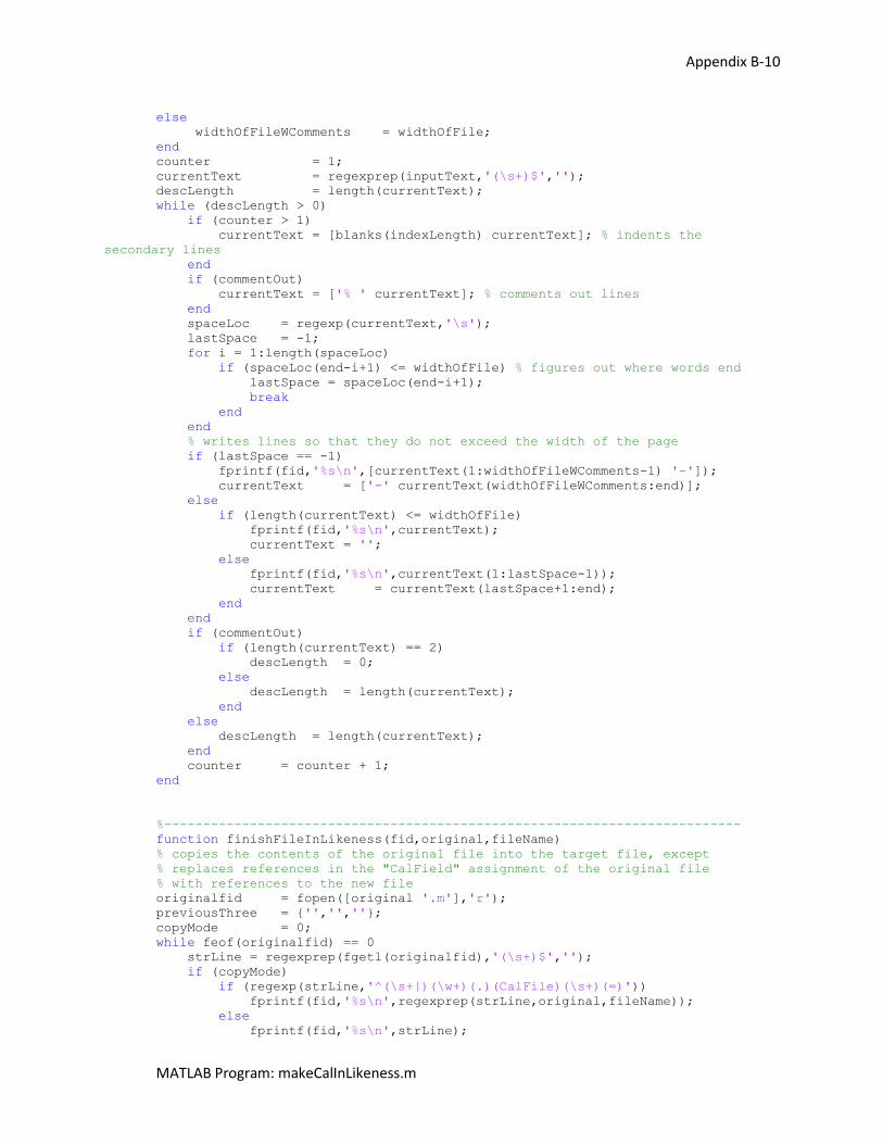
Appendix B-10
MATLAB Program: makeCalInLikeness.m
else
widthOfFileWComments = widthOfFile;
end
counter = 1;
currentText = regexprep(inputText,'(\s+)$','');
descLength = length(currentText);
while (descLength > 0)
if (counter > 1)
currentText = [blanks(indexLength) currentText]; % indents the
secondary lines
end
if (commentOut)
currentText = ['% ' currentText]; % comments out lines
end
spaceLoc = regexp(currentText,'\s');
lastSpace = -1;
for i = 1:length(spaceLoc)
if (spaceLoc(end-i+1) <= widthOfFile) % figures out where words end
lastSpace = spaceLoc(end-i+1);
break
end
end
% writes lines so that they do not exceed the width of the page
if (lastSpace == -1)
fprintf(fid,'%s\n',[currentText(1:widthOfFileWComments-1) '-']);
currentText = ['-' currentText(widthOfFileWComments:end)];
else
if (length(currentText) <= widthOfFile)
fprintf(fid,'%s\n',currentText);
currentText = '';
else
fprintf(fid,'%s\n',currentText(1:lastSpace-1));
currentText = currentText(lastSpace+1:end);
end
end
if (commentOut)
if (length(currentText) == 2)
descLength = 0;
else
descLength = length(currentText);
end
else
descLength = length(currentText);
end
counter = counter + 1;
end
%--------------------------------------------------------------------------
function finishFileInLikeness(fid,original,fileName)
% copies the contents of the original file into the target file, except
% replaces references in the "CalField" assignment of the original file
% with references to the new file
originalfid = fopen([original '.m'],'r');
previousThree = {'','',''};
copyMode = 0;
while feof(originalfid) == 0
strLine = regexprep(fgetl(originalfid),'(\s+)$','');
if (copyMode)
if (regexp(strLine,'^(\s+|)(\w+)(.)(CalFile)(\s+)(=)'))
fprintf(fid,'%s\n',regexprep(strLine,original,fileName));
else
fprintf(fid,'%s\n',strLine);
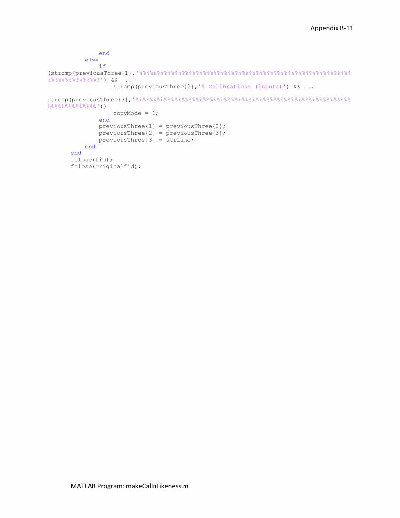
Appendix B-11
MATLAB Program: makeCalInLikeness.m
end
else
if
(strcmp(previousThree{1},'%%%%%%%%%%%%%%%%%%%%%%%%%%%%%%%%%%%%%%%%%%%%%%%%%%%%%%%%%%%%
%%%%%%%%%%%%%%%') && ...
strcmp(previousThree{2},'% Calibrations (inputs)') && ...
strcmp(previousThree{3},'%%%%%%%%%%%%%%%%%%%%%%%%%%%%%%%%%%%%%%%%%%%%%%%%%%%%%%%%%%%%%
%%%%%%%%%%%%%%'))
copyMode = 1;
end
previousThree{1} = previousThree{2};
previousThree{2} = previousThree{3};
previousThree{3} = strLine;
end
end
fclose(fid);
fclose(originalfid);
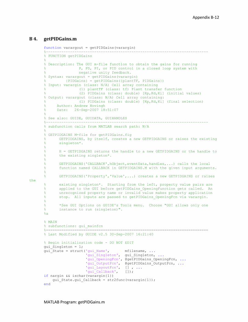
Appendix B-12
MATLAB Program: getPIDGains.m
B 4. getPIDGains.m
function varargout = getPIDGains(varargin)
%--------------------------------------------------------------------------
% FUNCTION getPIDGains
%
% Description: The GUI m-file function to obtain the gains for running
% P, PD, PI, or PID control in a closed loop system with
% negative unity feedback.
% Syntax: varargout = getPIDGains(varargin)
% {PIDGains} = getPIDGains({plantTF, PIDGains})
% Input: varargin (class: N/A) Cell array containing
% (1) plantTF (class: tf) Plant transfer function
% (2) PIDGains (class: double) [Kp,Kd,Ki] (initial values)
% Output: varargout (class: N/A) Cell array containing:
% (1) PIDGains (class: double) [Kp,Kd,Ki] (final selection)
% Author: Andrew Hovingh
% Date: 26-Sep-2007 18:51:07
%
% See also: GUIDE, GUIDATA, GUIHANDLES
%--------------------------------------------------------------------------
% subfunction calls from MATLAB search path: N/A
%
% GETPIDGAINS M-file for getPIDGains.fig
% GETPIDGAINS, by itself, creates a new GETPIDGAINS or raises the existing
% singleton*.
%
% H = GETPIDGAINS returns the handle to a new GETPIDGAINS or the handle to
% the existing singleton*.
%
% GETPIDGAINS('CALLBACK',hObject,eventData,handles,...) calls the local
% function named CALLBACK in GETPIDGAINS.M with the given input arguments.
%
% GETPIDGAINS('Property','Value',...) creates a new GETPIDGAINS or raises
the
% existing singleton*. Starting from the left, property value pairs are
% applied to the GUI before getPIDGains_OpeningFunction gets called. An
% unrecognized property name or invalid value makes property application
% stop. All inputs are passed to getPIDGains_OpeningFcn via varargin.
%
% *See GUI Options on GUIDE's Tools menu. Choose "GUI allows only one
% instance to run (singleton)".
%a
% MAIN
% subfunctions: gui_mainfcn
%==========================================================================
% Last Modified by GUIDE v2.5 30-Sep-2007 16:21:40
% Begin initialization code - DO NOT EDIT
gui_Singleton = 1;
gui_State = struct('gui_Name', mfilename, ...
'gui_Singleton', gui_Singleton, ...
'gui_OpeningFcn', @getPIDGains_OpeningFcn, ...
'gui_OutputFcn', @getPIDGains_OutputFcn, ...
'gui_LayoutFcn', [] , ...
'gui_Callback', []);
if nargin && ischar(varargin{1})
gui_State.gui_Callback = str2func(varargin{1});
end
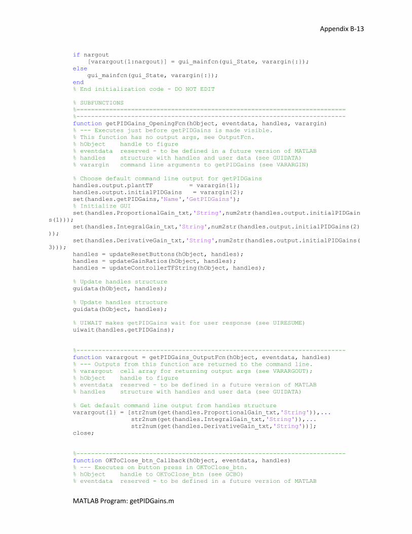
Appendix B-13
MATLAB Program: getPIDGains.m
if nargout
[varargout{1:nargout}] = gui_mainfcn(gui_State, varargin{:});
else
gui_mainfcn(gui_State, varargin{:});
end
% End initialization code - DO NOT EDIT
% SUBFUNCTIONS
%==========================================================================
%--------------------------------------------------------------------------
function getPIDGains_OpeningFcn(hObject, eventdata, handles, varargin)
% --- Executes just before getPIDGains is made visible.
% This function has no output args, see OutputFcn.
% hObject handle to figure
% eventdata reserved - to be defined in a future version of MATLAB
% handles structure with handles and user data (see GUIDATA)
% varargin command line arguments to getPIDGains (see VARARGIN)
% Choose default command line output for getPIDGains
handles.output.plantTF = varargin{1};
handles.output.initialPIDGains = varargin{2};
set(handles.getPIDGains,'Name','GetPIDGains');
% Initialize GUI
set(handles.ProportionalGain_txt,'String',num2str(handles.output.initialPIDGain
s(1)));
set(handles.IntegralGain_txt,'String',num2str(handles.output.initialPIDGains(2)
));
set(handles.DerivativeGain_txt,'String',num2str(handles.output.initialPIDGains(
3)));
handles = updateResetButtons(hObject, handles);
handles = updateGainRatios(hObject, handles);
handles = updateControllerTFString(hObject, handles);
% Update handles structure
guidata(hObject, handles);
% Update handles structure
guidata(hObject, handles);
% UIWAIT makes getPIDGains wait for user response (see UIRESUME)
uiwait(handles.getPIDGains);
%--------------------------------------------------------------------------
function varargout = getPIDGains_OutputFcn(hObject, eventdata, handles)
% --- Outputs from this function are returned to the command line.
% varargout cell array for returning output args (see VARARGOUT);
% hObject handle to figure
% eventdata reserved - to be defined in a future version of MATLAB
% handles structure with handles and user data (see GUIDATA)
% Get default command line output from handles structure
varargout{1} = [str2num(get(handles.ProportionalGain_txt,'String')),...
str2num(get(handles.IntegralGain_txt,'String')),...
str2num(get(handles.DerivativeGain_txt,'String'))];
close;
%--------------------------------------------------------------------------
function OKToClose_btn_Callback(hObject, eventdata, handles)
% --- Executes on button press in OKToClose_btn.
% hObject handle to OKToClose_btn (see GCBO)
% eventdata reserved - to be defined in a future version of MATLAB
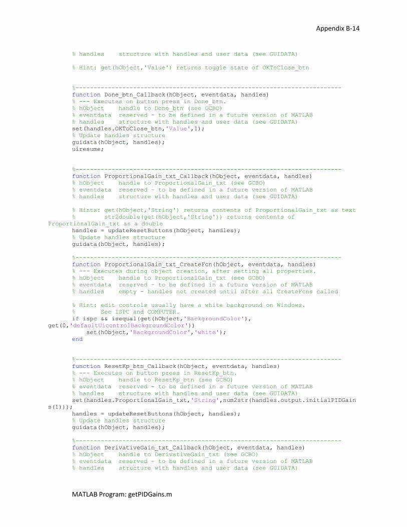
Appendix B-14
MATLAB Program: getPIDGains.m
% handles structure with handles and user data (see GUIDATA)
% Hint: get(hObject,'Value') returns toggle state of OKToClose_btn
%--------------------------------------------------------------------------
function Done_btn_Callback(hObject, eventdata, handles)
% --- Executes on button press in Done_btn.
% hObject handle to Done_btn (see GCBO)
% eventdata reserved - to be defined in a future version of MATLAB
% handles structure with handles and user data (see GUIDATA)
set(handles.OKToClose_btn,'Value',1);
% Update handles structure
guidata(hObject, handles);
uiresume;
%--------------------------------------------------------------------------
function ProportionalGain_txt_Callback(hObject, eventdata, handles)
% hObject handle to ProportionalGain_txt (see GCBO)
% eventdata reserved - to be defined in a future version of MATLAB
% handles structure with handles and user data (see GUIDATA)
% Hints: get(hObject,'String') returns contents of ProportionalGain_txt as text
% str2double(get(hObject,'String')) returns contents of
ProportionalGain_txt as a double
handles = updateResetButtons(hObject, handles);
% Update handles structure
guidata(hObject, handles);
%--------------------------------------------------------------------------
function ProportionalGain_txt_CreateFcn(hObject, eventdata, handles)
% --- Executes during object creation, after setting all properties.
% hObject handle to ProportionalGain_txt (see GCBO)
% eventdata reserved - to be defined in a future version of MATLAB
% handles empty - handles not created until after all CreateFcns called
% Hint: edit controls usually have a white background on Windows.
% See ISPC and COMPUTER.
if ispc && isequal(get(hObject,'BackgroundColor'),
get(0,'defaultUicontrolBackgroundColor'))
set(hObject,'BackgroundColor','white');
end
%--------------------------------------------------------------------------
function ResetKp_btn_Callback(hObject, eventdata, handles)
% --- Executes on button press in ResetKp_btn.
% hObject handle to ResetKp_btn (see GCBO)
% eventdata reserved - to be defined in a future version of MATLAB
% handles structure with handles and user data (see GUIDATA)
set(handles.ProportionalGain_txt,'String',num2str(handles.output.initialPIDGain
s(1)));
handles = updateResetButtons(hObject, handles);
% Update handles structure
guidata(hObject, handles);
%--------------------------------------------------------------------------
function DerivativeGain_txt_Callback(hObject, eventdata, handles)
% hObject handle to DerivativeGain_txt (see GCBO)
% eventdata reserved - to be defined in a future version of MATLAB
% handles structure with handles and user data (see GUIDATA)
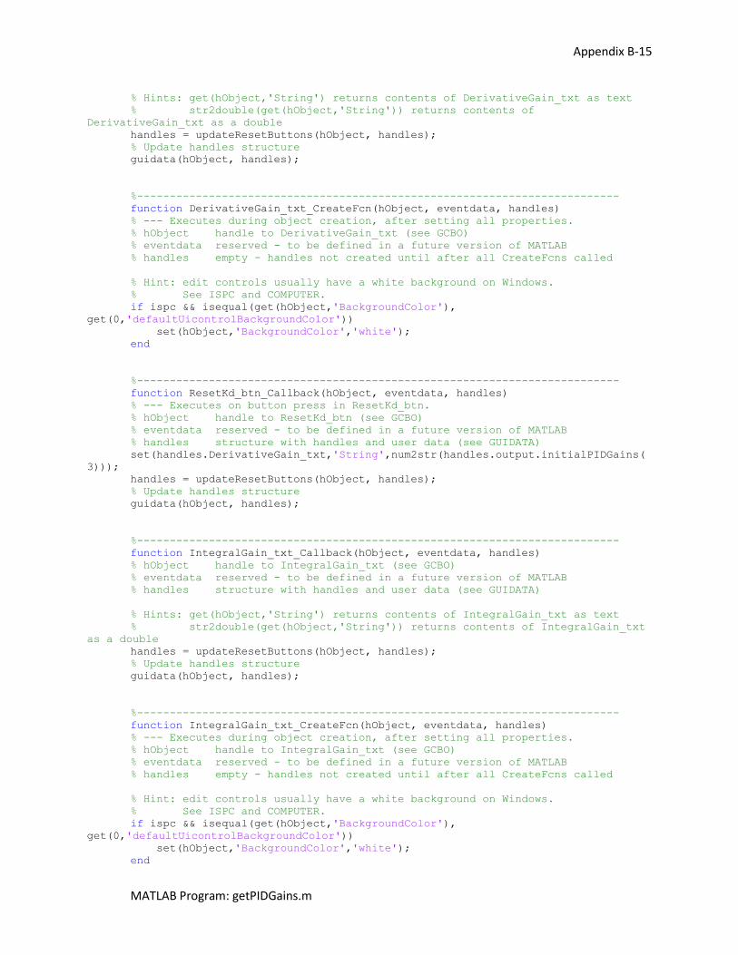
Appendix B-15
MATLAB Program: getPIDGains.m
% Hints: get(hObject,'String') returns contents of DerivativeGain_txt as text
% str2double(get(hObject,'String')) returns contents of
DerivativeGain_txt as a double
handles = updateResetButtons(hObject, handles);
% Update handles structure
guidata(hObject, handles);
%--------------------------------------------------------------------------
function DerivativeGain_txt_CreateFcn(hObject, eventdata, handles)
% --- Executes during object creation, after setting all properties.
% hObject handle to DerivativeGain_txt (see GCBO)
% eventdata reserved - to be defined in a future version of MATLAB
% handles empty - handles not created until after all CreateFcns called
% Hint: edit controls usually have a white background on Windows.
% See ISPC and COMPUTER.
if ispc && isequal(get(hObject,'BackgroundColor'),
get(0,'defaultUicontrolBackgroundColor'))
set(hObject,'BackgroundColor','white');
end
%--------------------------------------------------------------------------
function ResetKd_btn_Callback(hObject, eventdata, handles)
% --- Executes on button press in ResetKd_btn.
% hObject handle to ResetKd_btn (see GCBO)
% eventdata reserved - to be defined in a future version of MATLAB
% handles structure with handles and user data (see GUIDATA)
set(handles.DerivativeGain_txt,'String',num2str(handles.output.initialPIDGains(
3)));
handles = updateResetButtons(hObject, handles);
% Update handles structure
guidata(hObject, handles);
%--------------------------------------------------------------------------
function IntegralGain_txt_Callback(hObject, eventdata, handles)
% hObject handle to IntegralGain_txt (see GCBO)
% eventdata reserved - to be defined in a future version of MATLAB
% handles structure with handles and user data (see GUIDATA)
% Hints: get(hObject,'String') returns contents of IntegralGain_txt as text
% str2double(get(hObject,'String')) returns contents of IntegralGain_txt
as a double
handles = updateResetButtons(hObject, handles);
% Update handles structure
guidata(hObject, handles);
%--------------------------------------------------------------------------
function IntegralGain_txt_CreateFcn(hObject, eventdata, handles)
% --- Executes during object creation, after setting all properties.
% hObject handle to IntegralGain_txt (see GCBO)
% eventdata reserved - to be defined in a future version of MATLAB
% handles empty - handles not created until after all CreateFcns called
% Hint: edit controls usually have a white background on Windows.
% See ISPC and COMPUTER.
if ispc && isequal(get(hObject,'BackgroundColor'),
get(0,'defaultUicontrolBackgroundColor'))
set(hObject,'BackgroundColor','white');
end
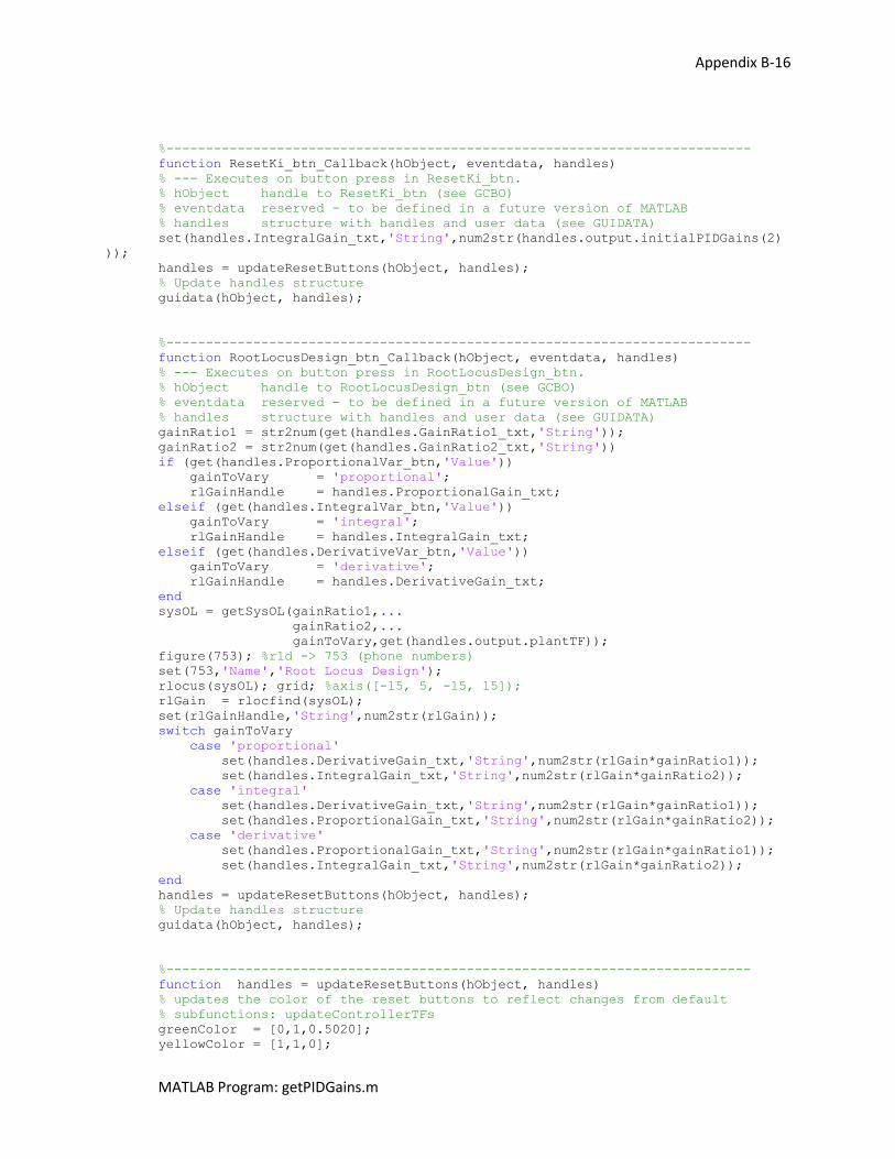
Appendix B-16
MATLAB Program: getPIDGains.m
%--------------------------------------------------------------------------
function ResetKi_btn_Callback(hObject, eventdata, handles)
% --- Executes on button press in ResetKi_btn.
% hObject handle to ResetKi_btn (see GCBO)
% eventdata reserved - to be defined in a future version of MATLAB
% handles structure with handles and user data (see GUIDATA)
set(handles.IntegralGain_txt,'String',num2str(handles.output.initialPIDGains(2)
));
handles = updateResetButtons(hObject, handles);
% Update handles structure
guidata(hObject, handles);
%--------------------------------------------------------------------------
function RootLocusDesign_btn_Callback(hObject, eventdata, handles)
% --- Executes on button press in RootLocusDesign_btn.
% hObject handle to RootLocusDesign_btn (see GCBO)
% eventdata reserved - to be defined in a future version of MATLAB
% handles structure with handles and user data (see GUIDATA)
gainRatio1 = str2num(get(handles.GainRatio1_txt,'String'));
gainRatio2 = str2num(get(handles.GainRatio2_txt,'String'))
if (get(handles.ProportionalVar_btn,'Value'))
gainToVary = 'proportional';
rlGainHandle = handles.ProportionalGain_txt;
elseif (get(handles.IntegralVar_btn,'Value'))
gainToVary = 'integral';
rlGainHandle = handles.IntegralGain_txt;
elseif (get(handles.DerivativeVar_btn,'Value'))
gainToVary = 'derivative';
rlGainHandle = handles.DerivativeGain_txt;
end
sysOL = getSysOL(gainRatio1,...
gainRatio2,...
gainToVary,get(handles.output.plantTF));
figure(753); %rld -> 753 (phone numbers)
set(753,'Name','Root Locus Design');
rlocus(sysOL); grid; %axis([-15, 5, -15, 15]);
rlGain = rlocfind(sysOL);
set(rlGainHandle,'String',num2str(rlGain));
switch gainToVary
case 'proportional'
set(handles.DerivativeGain_txt,'String',num2str(rlGain*gainRatio1));
set(handles.IntegralGain_txt,'String',num2str(rlGain*gainRatio2));
case 'integral'
set(handles.DerivativeGain_txt,'String',num2str(rlGain*gainRatio1));
set(handles.ProportionalGain_txt,'String',num2str(rlGain*gainRatio2));
case 'derivative'
set(handles.ProportionalGain_txt,'String',num2str(rlGain*gainRatio1));
set(handles.IntegralGain_txt,'String',num2str(rlGain*gainRatio2));
end
handles = updateResetButtons(hObject, handles);
% Update handles structure
guidata(hObject, handles);
%--------------------------------------------------------------------------
function handles = updateResetButtons(hObject, handles)
% updates the color of the reset buttons to reflect changes from default
% subfunctions: updateControllerTFs
greenColor = [0,1,0.5020];
yellowColor = [1,1,0];
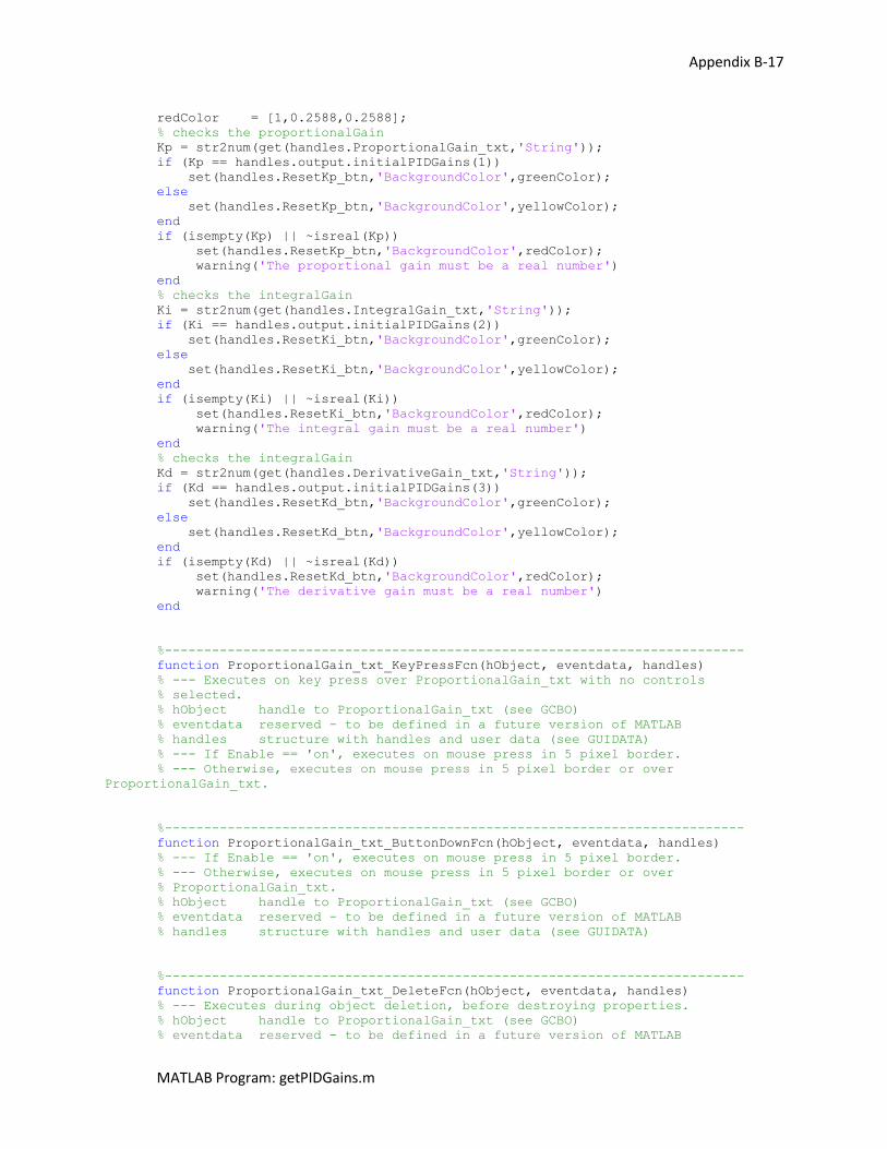
Appendix B-17
MATLAB Program: getPIDGains.m
redColor = [1,0.2588,0.2588];
% checks the proportionalGain
Kp = str2num(get(handles.ProportionalGain_txt,'String'));
if (Kp == handles.output.initialPIDGains(1))
set(handles.ResetKp_btn,'BackgroundColor',greenColor);
else
set(handles.ResetKp_btn,'BackgroundColor',yellowColor);
end
if (isempty(Kp) || ~isreal(Kp))
set(handles.ResetKp_btn,'BackgroundColor',redColor);
warning('The proportional gain must be a real number')
end
% checks the integralGain
Ki = str2num(get(handles.IntegralGain_txt,'String'));
if (Ki == handles.output.initialPIDGains(2))
set(handles.ResetKi_btn,'BackgroundColor',greenColor);
else
set(handles.ResetKi_btn,'BackgroundColor',yellowColor);
end
if (isempty(Ki) || ~isreal(Ki))
set(handles.ResetKi_btn,'BackgroundColor',redColor);
warning('The integral gain must be a real number')
end
% checks the integralGain
Kd = str2num(get(handles.DerivativeGain_txt,'String'));
if (Kd == handles.output.initialPIDGains(3))
set(handles.ResetKd_btn,'BackgroundColor',greenColor);
else
set(handles.ResetKd_btn,'BackgroundColor',yellowColor);
end
if (isempty(Kd) || ~isreal(Kd))
set(handles.ResetKd_btn,'BackgroundColor',redColor);
warning('The derivative gain must be a real number')
end
%--------------------------------------------------------------------------
function ProportionalGain_txt_KeyPressFcn(hObject, eventdata, handles)
% --- Executes on key press over ProportionalGain_txt with no controls
% selected.
% hObject handle to ProportionalGain_txt (see GCBO)
% eventdata reserved - to be defined in a future version of MATLAB
% handles structure with handles and user data (see GUIDATA)
% --- If Enable == 'on', executes on mouse press in 5 pixel border.
% --- Otherwise, executes on mouse press in 5 pixel border or over
ProportionalGain_txt.
%--------------------------------------------------------------------------
function ProportionalGain_txt_ButtonDownFcn(hObject, eventdata, handles)
% --- If Enable == 'on', executes on mouse press in 5 pixel border.
% --- Otherwise, executes on mouse press in 5 pixel border or over
% ProportionalGain_txt.
% hObject handle to ProportionalGain_txt (see GCBO)
% eventdata reserved - to be defined in a future version of MATLAB
% handles structure with handles and user data (see GUIDATA)
%--------------------------------------------------------------------------
function ProportionalGain_txt_DeleteFcn(hObject, eventdata, handles)
% --- Executes during object deletion, before destroying properties.
% hObject handle to ProportionalGain_txt (see GCBO)
% eventdata reserved - to be defined in a future version of MATLAB
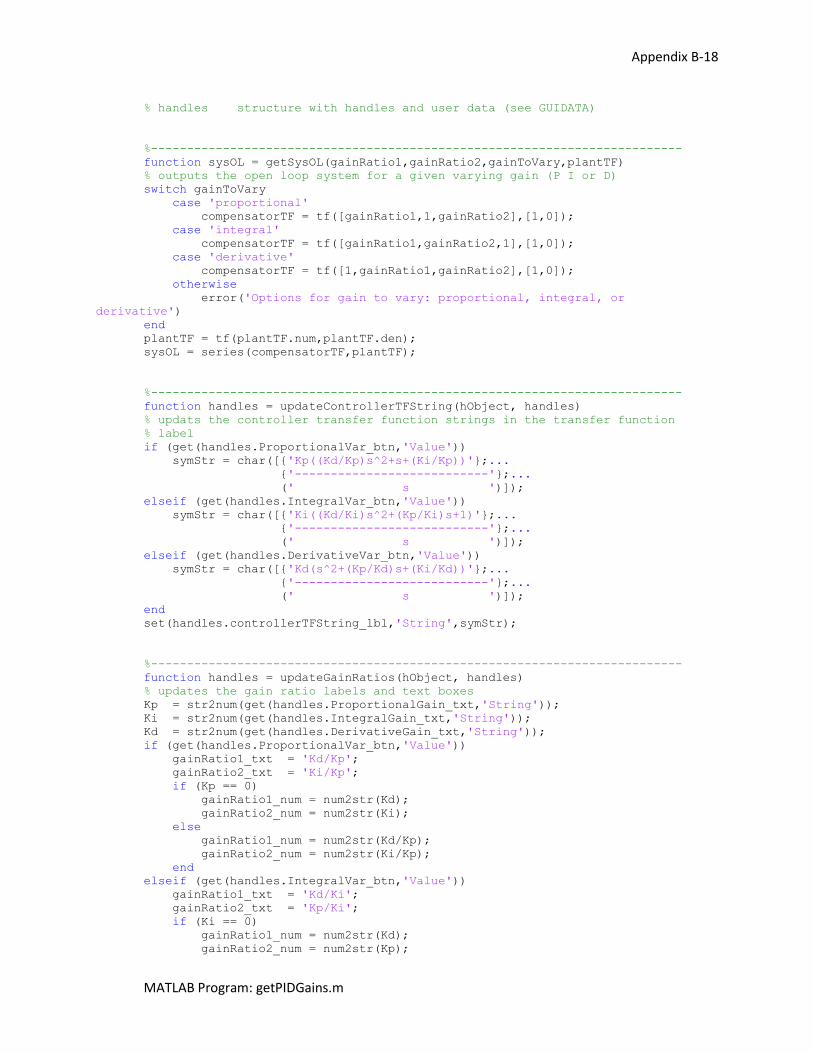
Appendix B-18
MATLAB Program: getPIDGains.m
% handles structure with handles and user data (see GUIDATA)
%--------------------------------------------------------------------------
function sysOL = getSysOL(gainRatio1,gainRatio2,gainToVary,plantTF)
% outputs the open loop system for a given varying gain (P I or D)
switch gainToVary
case 'proportional'
compensatorTF = tf([gainRatio1,1,gainRatio2],[1,0]);
case 'integral'
compensatorTF = tf([gainRatio1,gainRatio2,1],[1,0]);
case 'derivative'
compensatorTF = tf([1,gainRatio1,gainRatio2],[1,0]);
otherwise
error('Options for gain to vary: proportional, integral, or
derivative')
end
plantTF = tf(plantTF.num,plantTF.den);
sysOL = series(compensatorTF,plantTF);
%--------------------------------------------------------------------------
function handles = updateControllerTFString(hObject, handles)
% updats the controller transfer function strings in the transfer function
% label
if (get(handles.ProportionalVar_btn,'Value'))
symStr = char([{'Kp((Kd/Kp)s^2+s+(Ki/Kp))'};...
{'---------------------------'};...
(' s ')]);
elseif (get(handles.IntegralVar_btn,'Value'))
symStr = char([{'Ki((Kd/Ki)s^2+(Kp/Ki)s+1)'};...
{'---------------------------'};...
(' s ')]);
elseif (get(handles.DerivativeVar_btn,'Value'))
symStr = char([{'Kd(s^2+(Kp/Kd)s+(Ki/Kd))'};...
{'---------------------------'};...
(' s ')]);
end
set(handles.controllerTFString_lbl,'String',symStr);
%--------------------------------------------------------------------------
function handles = updateGainRatios(hObject, handles)
% updates the gain ratio labels and text boxes
Kp = str2num(get(handles.ProportionalGain_txt,'String'));
Ki = str2num(get(handles.IntegralGain_txt,'String'));
Kd = str2num(get(handles.DerivativeGain_txt,'String'));
if (get(handles.ProportionalVar_btn,'Value'))
gainRatio1_txt = 'Kd/Kp';
gainRatio2_txt = 'Ki/Kp';
if (Kp == 0)
gainRatio1_num = num2str(Kd);
gainRatio2_num = num2str(Ki);
else
gainRatio1_num = num2str(Kd/Kp);
gainRatio2_num = num2str(Ki/Kp);
end
elseif (get(handles.IntegralVar_btn,'Value'))
gainRatio1_txt = 'Kd/Ki';
gainRatio2_txt = 'Kp/Ki';
if (Ki == 0)
gainRatio1_num = num2str(Kd);
gainRatio2_num = num2str(Kp);
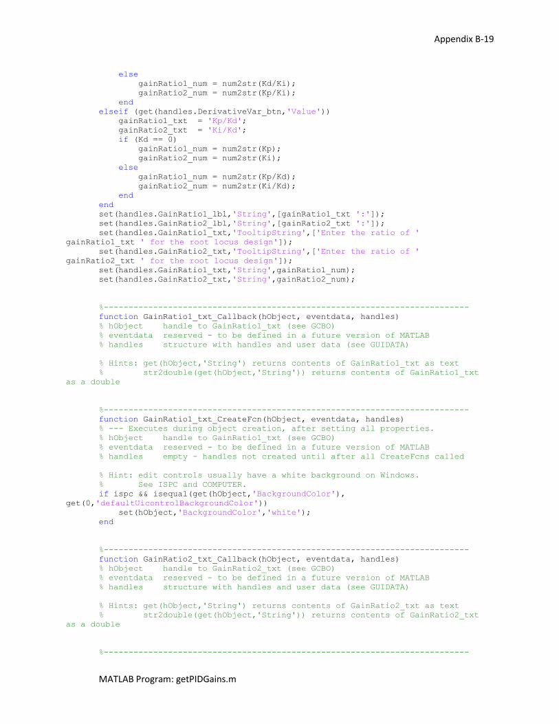
Appendix B-19
MATLAB Program: getPIDGains.m
else
gainRatio1_num = num2str(Kd/Ki);
gainRatio2_num = num2str(Kp/Ki);
end
elseif (get(handles.DerivativeVar_btn,'Value'))
gainRatio1_txt = 'Kp/Kd';
gainRatio2_txt = 'Ki/Kd';
if (Kd == 0)
gainRatio1_num = num2str(Kp);
gainRatio2_num = num2str(Ki);
else
gainRatio1_num = num2str(Kp/Kd);
gainRatio2_num = num2str(Ki/Kd);
end
end
set(handles.GainRatio1_lbl,'String',[gainRatio1_txt ':']);
set(handles.GainRatio2_lbl,'String',[gainRatio2_txt ':']);
set(handles.GainRatio1_txt,'TooltipString',['Enter the ratio of '
gainRatio1_txt ' for the root locus design']);
set(handles.GainRatio2_txt,'TooltipString',['Enter the ratio of '
gainRatio2_txt ' for the root locus design']);
set(handles.GainRatio1_txt,'String',gainRatio1_num);
set(handles.GainRatio2_txt,'String',gainRatio2_num);
%--------------------------------------------------------------------------
function GainRatio1_txt_Callback(hObject, eventdata, handles)
% hObject handle to GainRatio1_txt (see GCBO)
% eventdata reserved - to be defined in a future version of MATLAB
% handles structure with handles and user data (see GUIDATA)
% Hints: get(hObject,'String') returns contents of GainRatio1_txt as text
% str2double(get(hObject,'String')) returns contents of GainRatio1_txt
as a double
%--------------------------------------------------------------------------
function GainRatio1_txt_CreateFcn(hObject, eventdata, handles)
% --- Executes during object creation, after setting all properties.
% hObject handle to GainRatio1_txt (see GCBO)
% eventdata reserved - to be defined in a future version of MATLAB
% handles empty - handles not created until after all CreateFcns called
% Hint: edit controls usually have a white background on Windows.
% See ISPC and COMPUTER.
if ispc && isequal(get(hObject,'BackgroundColor'),
get(0,'defaultUicontrolBackgroundColor'))
set(hObject,'BackgroundColor','white');
end
%--------------------------------------------------------------------------
function GainRatio2_txt_Callback(hObject, eventdata, handles)
% hObject handle to GainRatio2_txt (see GCBO)
% eventdata reserved - to be defined in a future version of MATLAB
% handles structure with handles and user data (see GUIDATA)
% Hints: get(hObject,'String') returns contents of GainRatio2_txt as text
% str2double(get(hObject,'String')) returns contents of GainRatio2_txt
as a double
%--------------------------------------------------------------------------
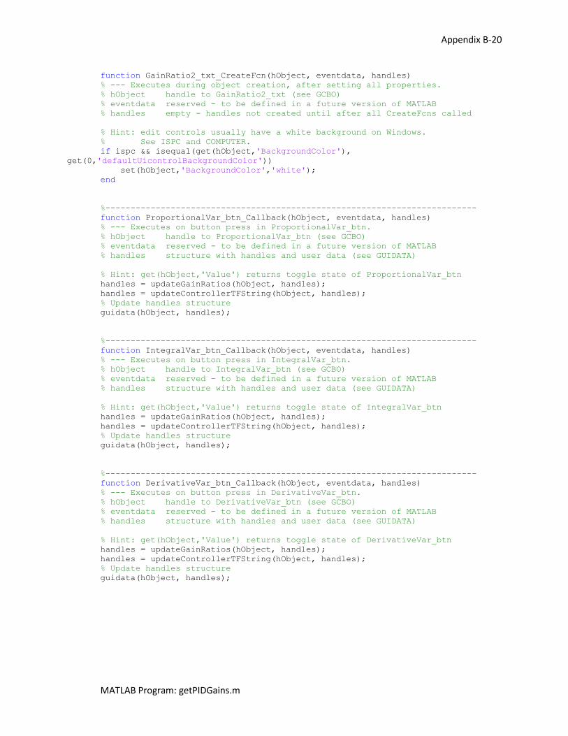
Appendix B-20
MATLAB Program: getPIDGains.m
function GainRatio2_txt_CreateFcn(hObject, eventdata, handles)
% --- Executes during object creation, after setting all properties.
% hObject handle to GainRatio2_txt (see GCBO)
% eventdata reserved - to be defined in a future version of MATLAB
% handles empty - handles not created until after all CreateFcns called
% Hint: edit controls usually have a white background on Windows.
% See ISPC and COMPUTER.
if ispc && isequal(get(hObject,'BackgroundColor'),
get(0,'defaultUicontrolBackgroundColor'))
set(hObject,'BackgroundColor','white');
end
%--------------------------------------------------------------------------
function ProportionalVar_btn_Callback(hObject, eventdata, handles)
% --- Executes on button press in ProportionalVar_btn.
% hObject handle to ProportionalVar_btn (see GCBO)
% eventdata reserved - to be defined in a future version of MATLAB
% handles structure with handles and user data (see GUIDATA)
% Hint: get(hObject,'Value') returns toggle state of ProportionalVar_btn
handles = updateGainRatios(hObject, handles);
handles = updateControllerTFString(hObject, handles);
% Update handles structure
guidata(hObject, handles);
%--------------------------------------------------------------------------
function IntegralVar_btn_Callback(hObject, eventdata, handles)
% --- Executes on button press in IntegralVar_btn.
% hObject handle to IntegralVar_btn (see GCBO)
% eventdata reserved - to be defined in a future version of MATLAB
% handles structure with handles and user data (see GUIDATA)
% Hint: get(hObject,'Value') returns toggle state of IntegralVar_btn
handles = updateGainRatios(hObject, handles);
handles = updateControllerTFString(hObject, handles);
% Update handles structure
guidata(hObject, handles);
%--------------------------------------------------------------------------
function DerivativeVar_btn_Callback(hObject, eventdata, handles)
% --- Executes on button press in DerivativeVar_btn.
% hObject handle to DerivativeVar_btn (see GCBO)
% eventdata reserved - to be defined in a future version of MATLAB
% handles structure with handles and user data (see GUIDATA)
% Hint: get(hObject,'Value') returns toggle state of DerivativeVar_btn
handles = updateGainRatios(hObject, handles);
handles = updateControllerTFString(hObject, handles);
% Update handles structure
guidata(hObject, handles);
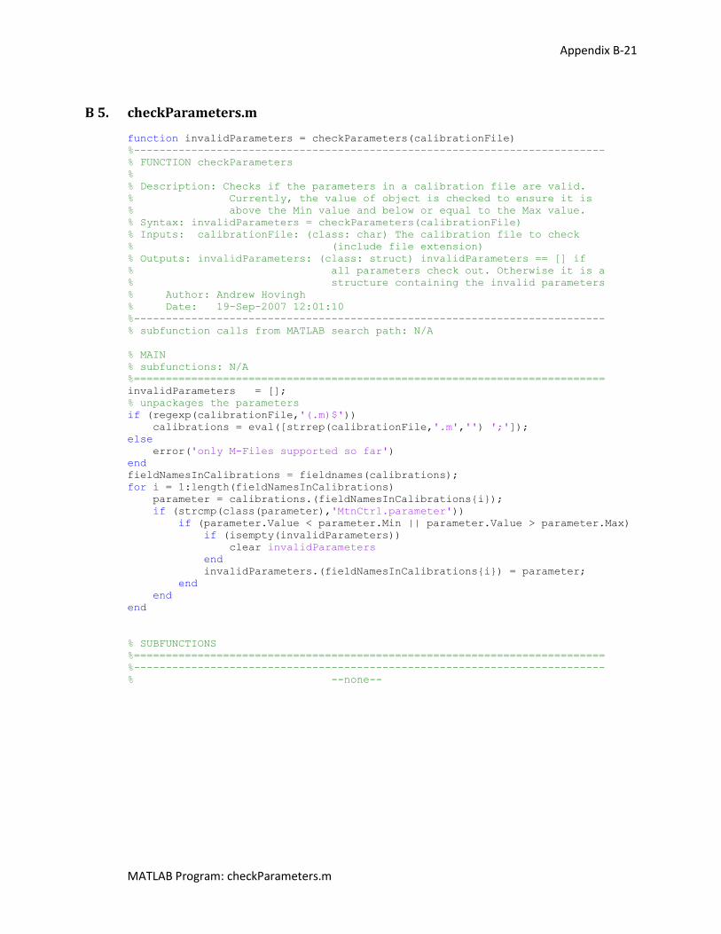
Appendix B-21
MATLAB Program: checkParameters.m
B 5. checkParameters.m
function invalidParameters = checkParameters(calibrationFile)
%--------------------------------------------------------------------------
% FUNCTION checkParameters
%
% Description: Checks if the parameters in a calibration file are valid.
% Currently, the value of object is checked to ensure it is
% above the Min value and below or equal to the Max value.
% Syntax: invalidParameters = checkParameters(calibrationFile)
% Inputs: calibrationFile: (class: char) The calibration file to check
% (include file extension)
% Outputs: invalidParameters: (class: struct) invalidParameters == [] if
% all parameters check out. Otherwise it is a
% structure containing the invalid parameters
% Author: Andrew Hovingh
% Date: 19-Sep-2007 12:01:10
%--------------------------------------------------------------------------
% subfunction calls from MATLAB search path: N/A
% MAIN
% subfunctions: N/A
%==========================================================================
invalidParameters = [];
% unpackages the parameters
if (regexp(calibrationFile,'(.m)$'))
calibrations = eval([strrep(calibrationFile,'.m','') ';']);
else
error('only M-Files supported so far')
end
fieldNamesInCalibrations = fieldnames(calibrations);
for i = 1:length(fieldNamesInCalibrations)
parameter = calibrations.(fieldNamesInCalibrations{i});
if (strcmp(class(parameter),'MtnCtrl.parameter'))
if (parameter.Value < parameter.Min || parameter.Value > parameter.Max)
if (isempty(invalidParameters))
clear invalidParameters
end
invalidParameters.(fieldNamesInCalibrations{i}) = parameter;
end
end
end
% SUBFUNCTIONS
%==========================================================================
%--------------------------------------------------------------------------
% --none--
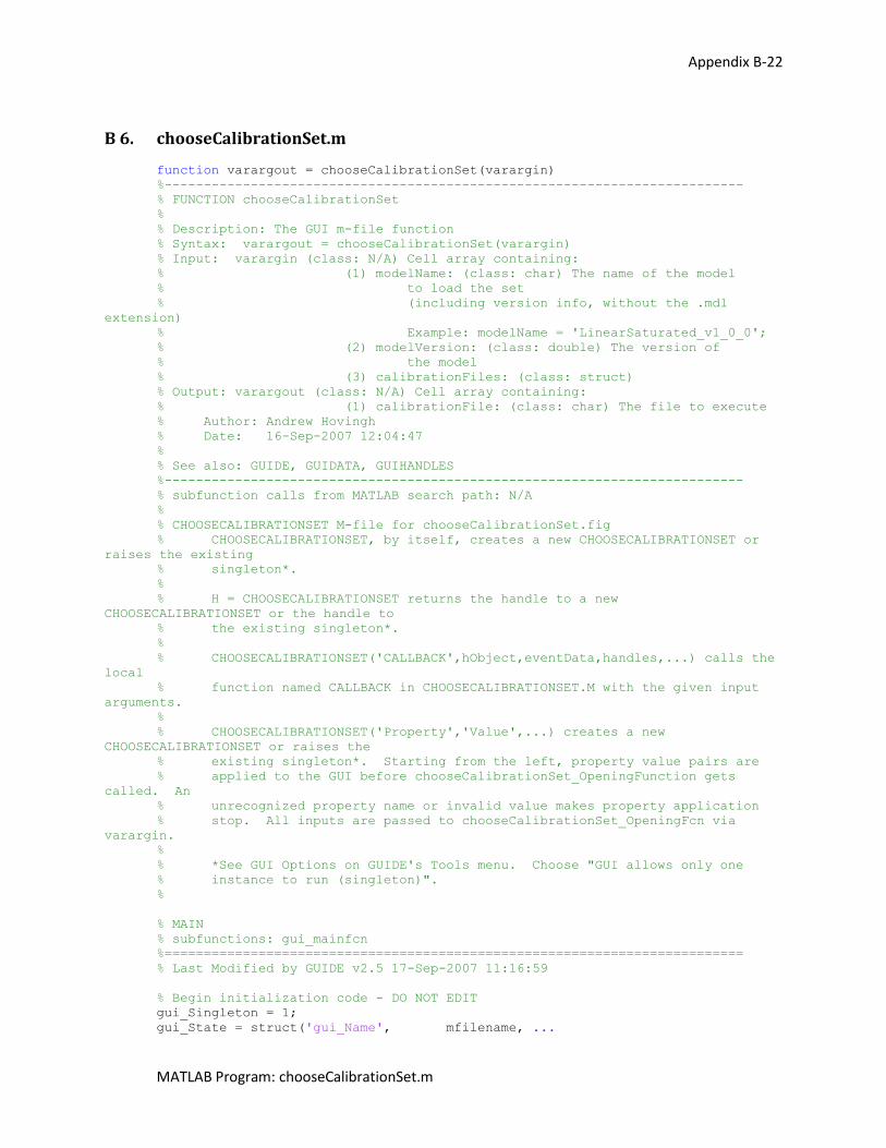
Appendix B-22
MATLAB Program: chooseCalibrationSet.m
B 6. chooseCalibrationSet.m
function varargout = chooseCalibrationSet(varargin)
%--------------------------------------------------------------------------
% FUNCTION chooseCalibrationSet
%
% Description: The GUI m-file function
% Syntax: varargout = chooseCalibrationSet(varargin)
% Input: varargin (class: N/A) Cell array containing:
% (1) modelName: (class: char) The name of the model
% to load the set
% (including version info, without the .mdl
extension)
% Example: modelName = 'LinearSaturated_v1_0_0';
% (2) modelVersion: (class: double) The version of
% the model
% (3) calibrationFiles: (class: struct)
% Output: varargout (class: N/A) Cell array containing:
% (1) calibrationFile: (class: char) The file to execute
% Author: Andrew Hovingh
% Date: 16-Sep-2007 12:04:47
%
% See also: GUIDE, GUIDATA, GUIHANDLES
%--------------------------------------------------------------------------
% subfunction calls from MATLAB search path: N/A
%
% CHOOSECALIBRATIONSET M-file for chooseCalibrationSet.fig
% CHOOSECALIBRATIONSET, by itself, creates a new CHOOSECALIBRATIONSET or
raises the existing
% singleton*.
%
% H = CHOOSECALIBRATIONSET returns the handle to a new
CHOOSECALIBRATIONSET or the handle to
% the existing singleton*.
%
% CHOOSECALIBRATIONSET('CALLBACK',hObject,eventData,handles,...) calls the
local
% function named CALLBACK in CHOOSECALIBRATIONSET.M with the given input
arguments.
%
% CHOOSECALIBRATIONSET('Property','Value',...) creates a new
CHOOSECALIBRATIONSET or raises the
% existing singleton*. Starting from the left, property value pairs are
% applied to the GUI before chooseCalibrationSet_OpeningFunction gets
called. An
% unrecognized property name or invalid value makes property application
% stop. All inputs are passed to chooseCalibrationSet_OpeningFcn via
varargin.
%
% *See GUI Options on GUIDE's Tools menu. Choose "GUI allows only one
% instance to run (singleton)".
%
% MAIN
% subfunctions: gui_mainfcn
%==========================================================================
% Last Modified by GUIDE v2.5 17-Sep-2007 11:16:59
% Begin initialization code - DO NOT EDIT
gui_Singleton = 1;
gui_State = struct('gui_Name', mfilename, ...
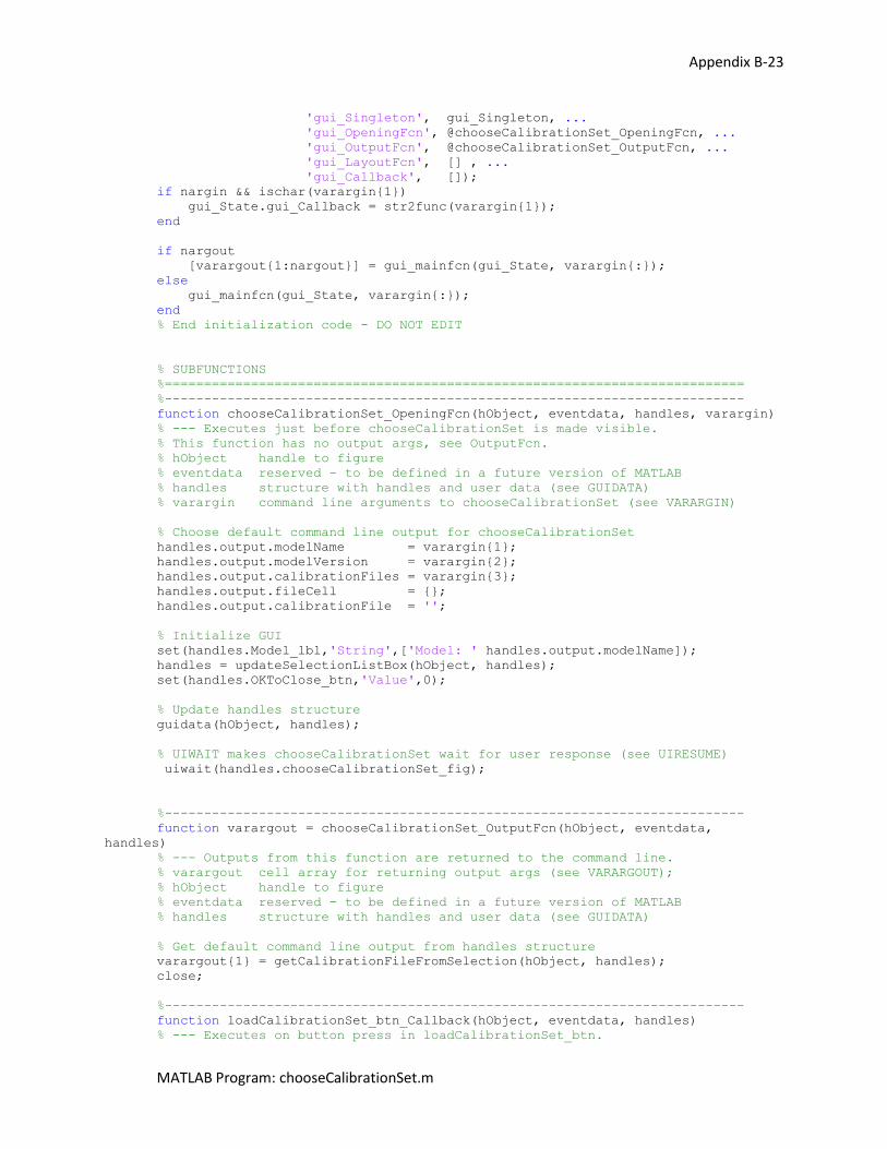
Appendix B-23
MATLAB Program: chooseCalibrationSet.m
'gui_Singleton', gui_Singleton, ...
'gui_OpeningFcn', @chooseCalibrationSet_OpeningFcn, ...
'gui_OutputFcn', @chooseCalibrationSet_OutputFcn, ...
'gui_LayoutFcn', [] , ...
'gui_Callback', []);
if nargin && ischar(varargin{1})
gui_State.gui_Callback = str2func(varargin{1});
end
if nargout
[varargout{1:nargout}] = gui_mainfcn(gui_State, varargin{:});
else
gui_mainfcn(gui_State, varargin{:});
end
% End initialization code - DO NOT EDIT
% SUBFUNCTIONS
%==========================================================================
%--------------------------------------------------------------------------
function chooseCalibrationSet_OpeningFcn(hObject, eventdata, handles, varargin)
% --- Executes just before chooseCalibrationSet is made visible.
% This function has no output args, see OutputFcn.
% hObject handle to figure
% eventdata reserved - to be defined in a future version of MATLAB
% handles structure with handles and user data (see GUIDATA)
% varargin command line arguments to chooseCalibrationSet (see VARARGIN)
% Choose default command line output for chooseCalibrationSet
handles.output.modelName = varargin{1};
handles.output.modelVersion = varargin{2};
handles.output.calibrationFiles = varargin{3};
handles.output.fileCell = {};
handles.output.calibrationFile = '';
% Initialize GUI
set(handles.Model_lbl,'String',['Model: ' handles.output.modelName]);
handles = updateSelectionListBox(hObject, handles);
set(handles.OKToClose_btn,'Value',0);
% Update handles structure
guidata(hObject, handles);
% UIWAIT makes chooseCalibrationSet wait for user response (see UIRESUME)
uiwait(handles.chooseCalibrationSet_fig);
%--------------------------------------------------------------------------
function varargout = chooseCalibrationSet_OutputFcn(hObject, eventdata,
handles)
% --- Outputs from this function are returned to the command line.
% varargout cell array for returning output args (see VARARGOUT);
% hObject handle to figure
% eventdata reserved - to be defined in a future version of MATLAB
% handles structure with handles and user data (see GUIDATA)
% Get default command line output from handles structure
varargout{1} = getCalibrationFileFromSelection(hObject, handles);
close;
%--------------------------------------------------------------------------
function loadCalibrationSet_btn_Callback(hObject, eventdata, handles)
% --- Executes on button press in loadCalibrationSet_btn.
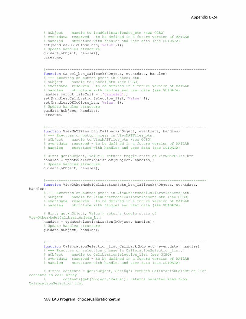
Appendix B-24
MATLAB Program: chooseCalibrationSet.m
% hObject handle to loadCalibrationSet_btn (see GCBO)
% eventdata reserved - to be defined in a future version of MATLAB
% handles structure with handles and user data (see GUIDATA)
set(handles.OKToClose_btn,'Value',1);
% Update handles structure
guidata(hObject, handles);
uiresume;
%--------------------------------------------------------------------------
function Cancel_btn_Callback(hObject, eventdata, handles)
% --- Executes on button press in Cancel_btn.
% hObject handle to Cancel_btn (see GCBO)
% eventdata reserved - to be defined in a future version of MATLAB
% handles structure with handles and user data (see GUIDATA)
handles.output.fileCell = {'canceled'};
set(handles.CalibrationSelection_list,'Value',1);
set(handles.OKToClose_btn,'Value',1);
% Update handles structure
guidata(hObject, handles);
uiresume;
%--------------------------------------------------------------------------
function ViewMATFiles_btn_Callback(hObject, eventdata, handles)
% --- Executes on button press in ViewMATFiles_btn.
% hObject handle to ViewMATFiles_btn (see GCBO)
% eventdata reserved - to be defined in a future version of MATLAB
% handles structure with handles and user data (see GUIDATA)
% Hint: get(hObject,'Value') returns toggle state of ViewMATFiles_btn
handles = updateSelectionListBox(hObject, handles);
% Update handles structure
guidata(hObject, handles);
%--------------------------------------------------------------------------
function ViewOtherModelCalibrationSets_btn_Callback(hObject, eventdata,
handles)
% --- Executes on button press in ViewOtherModelCalibrationSets_btn.
% hObject handle to ViewOtherModelCalibrationSets_btn (see GCBO)
% eventdata reserved - to be defined in a future version of MATLAB
% handles structure with handles and user data (see GUIDATA)
% Hint: get(hObject,'Value') returns toggle state of
ViewOtherModelCalibrationSets_btn
handles = updateSelectionListBox(hObject, handles);
% Update handles structure
guidata(hObject, handles);
%--------------------------------------------------------------------------
function CalibrationSelection_list_Callback(hObject, eventdata, handles)
% --- Executes on selection change in CalibrationSelection_list.
% hObject handle to CalibrationSelection_list (see GCBO)
% eventdata reserved - to be defined in a future version of MATLAB
% handles structure with handles and user data (see GUIDATA)
% Hints: contents = get(hObject,'String') returns CalibrationSelection_list
contents as cell array
% contents{get(hObject,'Value')} returns selected item from
CalibrationSelection_list
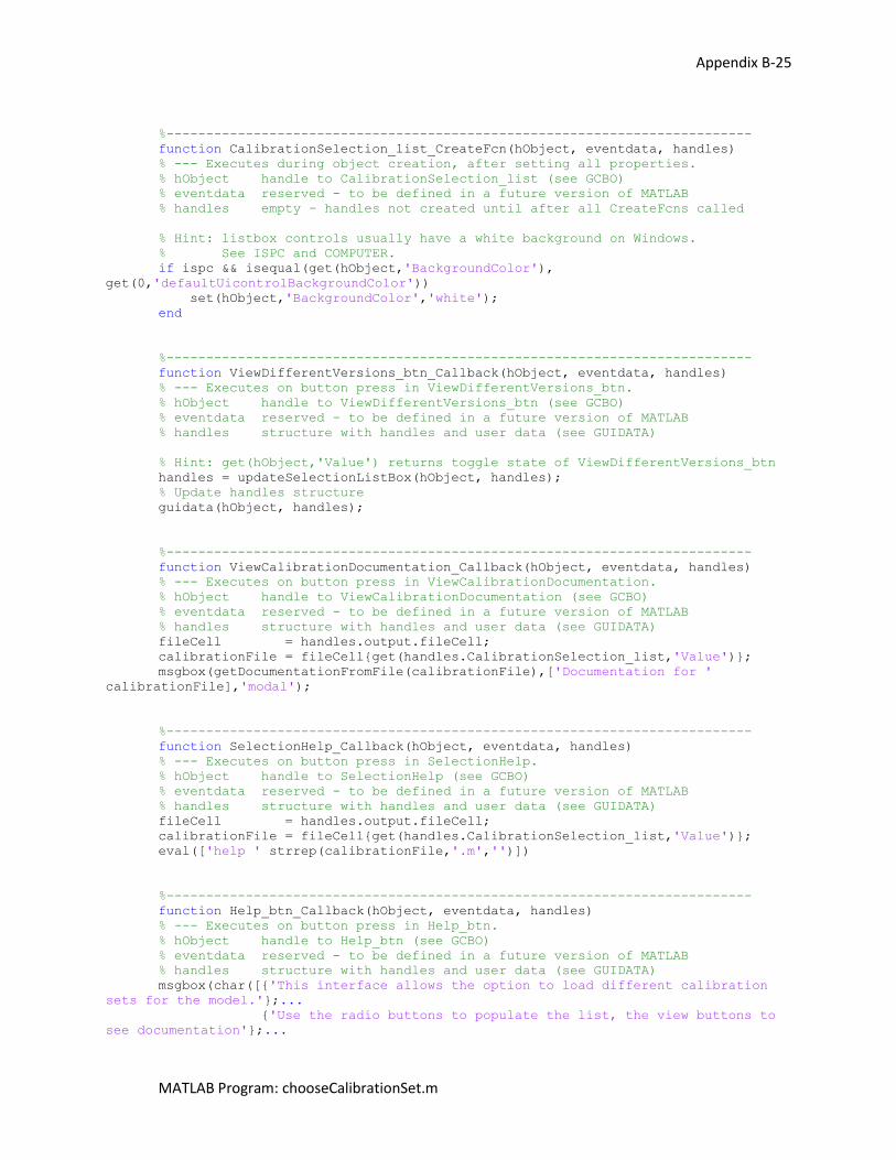
Appendix B-25
MATLAB Program: chooseCalibrationSet.m
%--------------------------------------------------------------------------
function CalibrationSelection_list_CreateFcn(hObject, eventdata, handles)
% --- Executes during object creation, after setting all properties.
% hObject handle to CalibrationSelection_list (see GCBO)
% eventdata reserved - to be defined in a future version of MATLAB
% handles empty - handles not created until after all CreateFcns called
% Hint: listbox controls usually have a white background on Windows.
% See ISPC and COMPUTER.
if ispc && isequal(get(hObject,'BackgroundColor'),
get(0,'defaultUicontrolBackgroundColor'))
set(hObject,'BackgroundColor','white');
end
%--------------------------------------------------------------------------
function ViewDifferentVersions_btn_Callback(hObject, eventdata, handles)
% --- Executes on button press in ViewDifferentVersions_btn.
% hObject handle to ViewDifferentVersions_btn (see GCBO)
% eventdata reserved - to be defined in a future version of MATLAB
% handles structure with handles and user data (see GUIDATA)
% Hint: get(hObject,'Value') returns toggle state of ViewDifferentVersions_btn
handles = updateSelectionListBox(hObject, handles);
% Update handles structure
guidata(hObject, handles);
%--------------------------------------------------------------------------
function ViewCalibrationDocumentation_Callback(hObject, eventdata, handles)
% --- Executes on button press in ViewCalibrationDocumentation.
% hObject handle to ViewCalibrationDocumentation (see GCBO)
% eventdata reserved - to be defined in a future version of MATLAB
% handles structure with handles and user data (see GUIDATA)
fileCell = handles.output.fileCell;
calibrationFile = fileCell{get(handles.CalibrationSelection_list,'Value')};
msgbox(getDocumentationFromFile(calibrationFile),['Documentation for '
calibrationFile],'modal');
%--------------------------------------------------------------------------
function SelectionHelp_Callback(hObject, eventdata, handles)
% --- Executes on button press in SelectionHelp.
% hObject handle to SelectionHelp (see GCBO)
% eventdata reserved - to be defined in a future version of MATLAB
% handles structure with handles and user data (see GUIDATA)
fileCell = handles.output.fileCell;
calibrationFile = fileCell{get(handles.CalibrationSelection_list,'Value')};
eval(['help ' strrep(calibrationFile,'.m','')])
%--------------------------------------------------------------------------
function Help_btn_Callback(hObject, eventdata, handles)
% --- Executes on button press in Help_btn.
% hObject handle to Help_btn (see GCBO)
% eventdata reserved - to be defined in a future version of MATLAB
% handles structure with handles and user data (see GUIDATA)
msgbox(char([{'This interface allows the option to load different calibration
sets for the model.'};...
{'Use the radio buttons to populate the list, the view buttons to
see documentation'};...
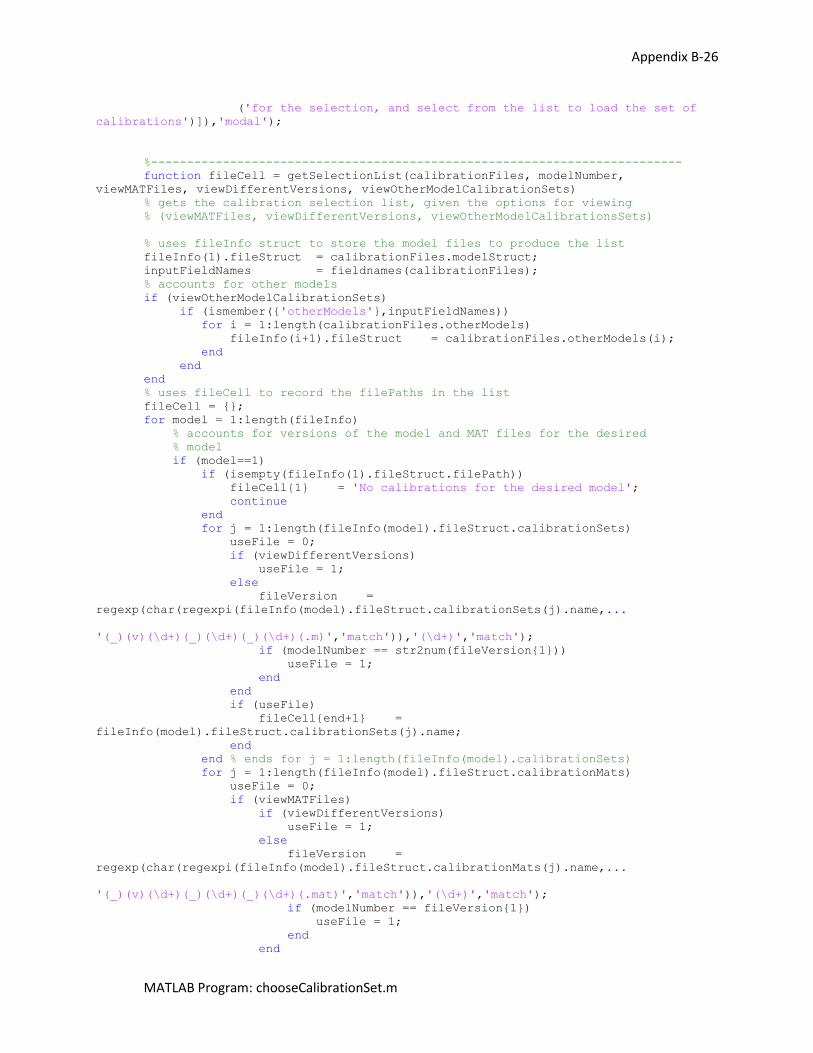
Appendix B-26
MATLAB Program: chooseCalibrationSet.m
('for the selection, and select from the list to load the set of
calibrations')]),'modal');
%--------------------------------------------------------------------------
function fileCell = getSelectionList(calibrationFiles, modelNumber,
viewMATFiles, viewDifferentVersions, viewOtherModelCalibrationSets)
% gets the calibration selection list, given the options for viewing
% (viewMATFiles, viewDifferentVersions, viewOtherModelCalibrationsSets)
% uses fileInfo struct to store the model files to produce the list
fileInfo(1).fileStruct = calibrationFiles.modelStruct;
inputFieldNames = fieldnames(calibrationFiles);
% accounts for other models
if (viewOtherModelCalibrationSets)
if (ismember({'otherModels'},inputFieldNames))
for i = 1:length(calibrationFiles.otherModels)
fileInfo(i+1).fileStruct = calibrationFiles.otherModels(i);
end
end
end
% uses fileCell to record the filePaths in the list
fileCell = {};
for model = 1:length(fileInfo)
% accounts for versions of the model and MAT files for the desired
% model
if (model==1)
if (isempty(fileInfo(1).fileStruct.filePath))
fileCell{1} = 'No calibrations for the desired model';
continue
end
for j = 1:length(fileInfo(model).fileStruct.calibrationSets)
useFile = 0;
if (viewDifferentVersions)
useFile = 1;
else
fileVersion =
regexp(char(regexpi(fileInfo(model).fileStruct.calibrationSets(j).name,...
'(_)(v)(\d+)(_)(\d+)(_)(\d+)(.m)','match')),'(\d+)','match');
if (modelNumber == str2num(fileVersion{1}))
useFile = 1;
end
end
if (useFile)
fileCell{end+1} =
fileInfo(model).fileStruct.calibrationSets(j).name;
end
end % ends for j = 1:length(fileInfo(model).calibrationSets)
for j = 1:length(fileInfo(model).fileStruct.calibrationMats)
useFile = 0;
if (viewMATFiles)
if (viewDifferentVersions)
useFile = 1;
else
fileVersion =
regexp(char(regexpi(fileInfo(model).fileStruct.calibrationMats(j).name,...
'(_)(v)(\d+)(_)(\d+)(_)(\d+)(.mat)','match')),'(\d+)','match');
if (modelNumber == fileVersion{1})
useFile = 1;
end
end
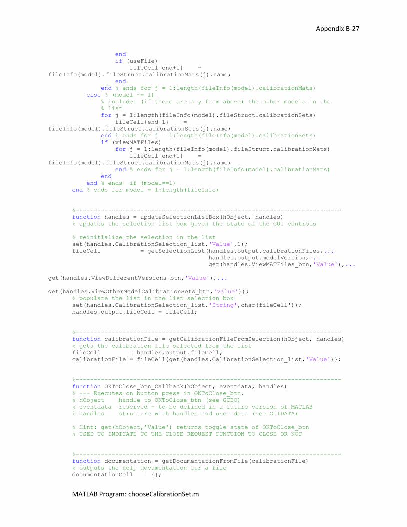
Appendix B-27
MATLAB Program: chooseCalibrationSet.m
end
if (useFile)
fileCell{end+1} =
fileInfo(model).fileStruct.calibrationMats(j).name;
end
end % ends for j = 1:length(fileInfo(model).calibrationMats)
else % (model ~= 1)
% includes (if there are any from above) the other models in the
% list
for j = 1:length(fileInfo(model).fileStruct.calibrationSets)
fileCell{end+1} =
fileInfo(model).fileStruct.calibrationSets(j).name;
end % ends for j = 1:length(fileInfo(model).calibrationSets)
if (viewMATFiles)
for j = 1:length(fileInfo(model).fileStruct.calibrationMats)
fileCell{end+1} =
fileInfo(model).fileStruct.calibrationMats(j).name;
end % ends for j = 1:length(fileInfo(model).calibrationMats)
end
end % ends if (model==1)
end % ends for model = 1:length(fileInfo)
%--------------------------------------------------------------------------
function handles = updateSelectionListBox(hObject, handles)
% updates the selection list box given the state of the GUI controls
% reinitialize the selection in the list
set(handles.CalibrationSelection_list,'Value',1);
fileCell = getSelectionList(handles.output.calibrationFiles,...
handles.output.modelVersion,...
get(handles.ViewMATFiles_btn,'Value'),...
get(handles.ViewDifferentVersions_btn,'Value'),...
get(handles.ViewOtherModelCalibrationSets_btn,'Value'));
% populate the list in the list selection box
set(handles.CalibrationSelection_list,'String',char(fileCell'));
handles.output.fileCell = fileCell;
%--------------------------------------------------------------------------
function calibrationFile = getCalibrationFileFromSelection(hObject, handles)
% gets the calibration file selected from the list
fileCell = handles.output.fileCell;
calibrationFile = fileCell{get(handles.CalibrationSelection_list,'Value')};
%--------------------------------------------------------------------------
function OKToClose_btn_Callback(hObject, eventdata, handles)
% --- Executes on button press in OKToClose_btn.
% hObject handle to OKToClose_btn (see GCBO)
% eventdata reserved - to be defined in a future version of MATLAB
% handles structure with handles and user data (see GUIDATA)
% Hint: get(hObject,'Value') returns toggle state of OKToClose_btn
% USED TO INDICATE TO THE CLOSE REQUEST FUNCTION TO CLOSE OR NOT
%--------------------------------------------------------------------------
function documentation = getDocumentationFromFile(calibrationFile)
% outputs the help documentation for a file
documentationCell = {};
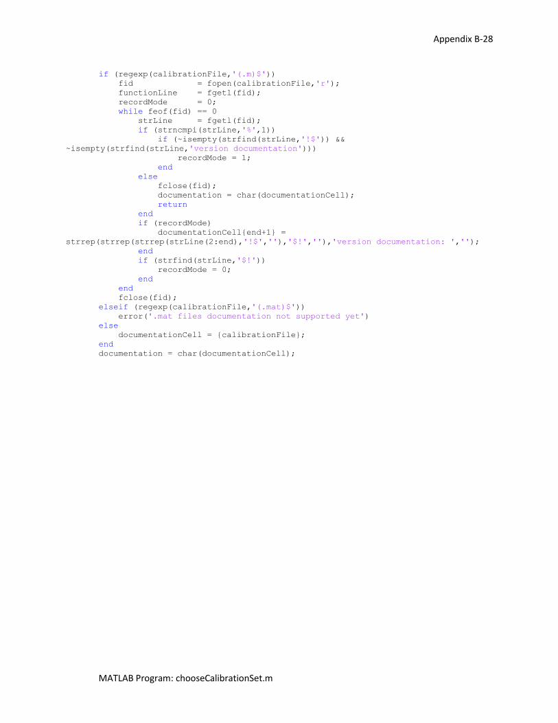
Appendix B-28
MATLAB Program: chooseCalibrationSet.m
if (regexp(calibrationFile,'(.m)$'))
fid = fopen(calibrationFile,'r');
functionLine = fgetl(fid);
recordMode = 0;
while feof(fid) == 0
strLine = fgetl(fid);
if (strncmpi(strLine,'%',1))
if (~isempty(strfind(strLine,'!$')) &&
~isempty(strfind(strLine,'version documentation')))
recordMode = 1;
end
else
fclose(fid);
documentation = char(documentationCell);
return
end
if (recordMode)
documentationCell{end+1} =
strrep(strrep(strrep(strLine(2:end),'!$',''),'$!',''),'version documentation: ','');
end
if (strfind(strLine,'$!'))
recordMode = 0;
end
end
fclose(fid);
elseif (regexp(calibrationFile,'(.mat)$'))
error('.mat files documentation not supported yet')
else
documentationCell = {calibrationFile};
end
documentation = char(documentationCell);
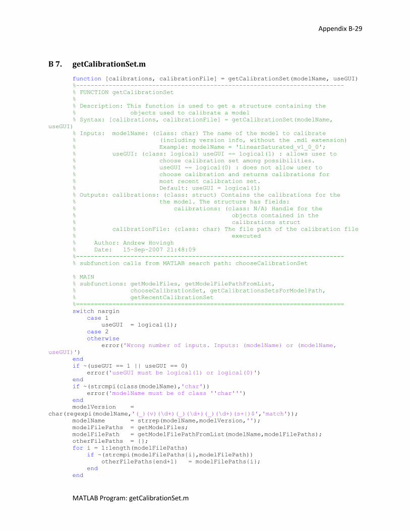
Appendix B-29
MATLAB Program: getCalibrationSet.m
B 7. getCalibrationSet.m
function [calibrations, calibrationFile] = getCalibrationSet(modelName, useGUI)
%--------------------------------------------------------------------------
% FUNCTION getCalibrationSet
%
% Description: This function is used to get a structure containing the
% objects used to calibrate a model
% Syntax: [calibrations, calibrationFile] = getCalibrationSet(modelName,
useGUI)
% Inputs: modelName: (class: char) The name of the model to calibrate
% (including version info, without the .mdl extension)
% Example: modelName = 'LinearSaturated_v1_0_0';
% useGUI: (class: logical) useGUI == logical(1) : allows user to
% choose calibration set among possibilities.
% useGUI == logical(0) : does not allow user to
% choose calibration and returns calibrations for
% most recent calibration set.
% Default: useGUI = logical(1)
% Outputs: calibrations: (class: struct) Contains the calibrations for the
% the model. The structure has fields:
% calibrations: (class: N/A) Handle for the
% objects contained in the
% calibrations struct
% calibrationFile: (class: char) The file path of the calibration file
% executed
% Author: Andrew Hovingh
% Date: 15-Sep-2007 21:48:09
%--------------------------------------------------------------------------
% subfunction calls from MATLAB search path: chooseCalibrationSet
% MAIN
% subfunctions: getModelFiles, getModelFilePathFromList,
% chooseCalibrationSet, getCalibrationsSetsForModelPath,
% getRecentCalibrationSet
%==========================================================================
switch nargin
case 1
useGUI = logical(1);
case 2
otherwise
error('Wrong number of inputs. Inputs: (modelName) or (modelName,
useGUI)')
end
if ~(useGUI == 1 || useGUI == 0)
error('useGUI must be logical(1) or logical(0)')
end
if ~(strcmpi(class(modelName),'char'))
error('modelName must be of class ''char''')
end
modelVersion =
char(regexpi(modelName,'(_)(v)(\d+)(_)(\d+)(_)(\d+)(s+|)$','match'));
modelName = strrep(modelName,modelVersion,'');
modelFilePaths = getModelFiles;
modelFilePath = getModelFilePathFromList(modelName,modelFilePaths);
otherFilePaths = {};
for i = 1:length(modelFilePaths)
if ~(strcmpi(modelFilePaths{i},modelFilePath))
otherFilePaths{end+1} = modelFilePaths{i};
end
end
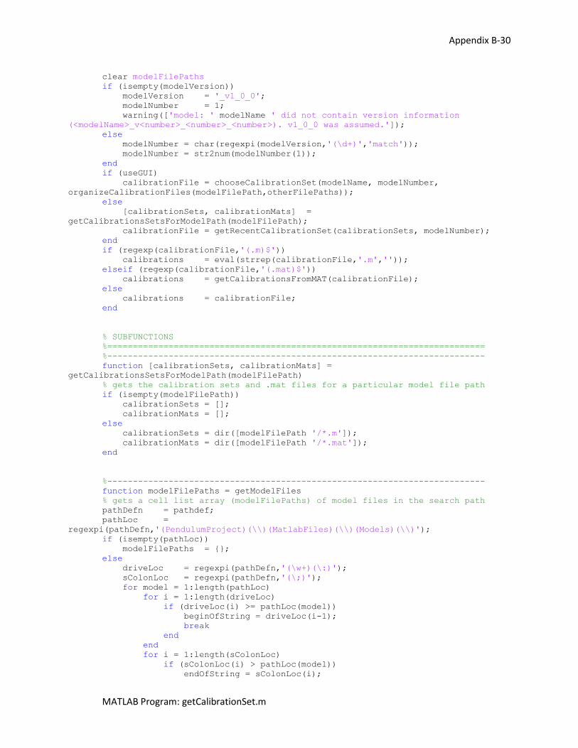
Appendix B-30
MATLAB Program: getCalibrationSet.m
clear modelFilePaths
if (isempty(modelVersion))
modelVersion = '_v1_0_0';
modelNumber = 1;
warning(['model: ' modelName ' did not contain version information
(<modelName>_v<number>_<number>_<number>). v1_0_0 was assumed.']);
else
modelNumber = char(regexpi(modelVersion,'(\d+)','match'));
modelNumber = str2num(modelNumber(1));
end
if (useGUI)
calibrationFile = chooseCalibrationSet(modelName, modelNumber,
organizeCalibrationFiles(modelFilePath,otherFilePaths));
else
[calibrationSets, calibrationMats] =
getCalibrationsSetsForModelPath(modelFilePath);
calibrationFile = getRecentCalibrationSet(calibrationSets, modelNumber);
end
if (regexp(calibrationFile,'(.m)$'))
calibrations = eval(strrep(calibrationFile,'.m',''));
elseif (regexp(calibrationFile,'(.mat)$'))
calibrations = getCalibrationsFromMAT(calibrationFile);
else
calibrations = calibrationFile;
end
% SUBFUNCTIONS
%==========================================================================
%--------------------------------------------------------------------------
function [calibrationSets, calibrationMats] =
getCalibrationsSetsForModelPath(modelFilePath)
% gets the calibration sets and .mat files for a particular model file path
if (isempty(modelFilePath))
calibrationSets = [];
calibrationMats = [];
else
calibrationSets = dir([modelFilePath '/*.m']);
calibrationMats = dir([modelFilePath '/*.mat']);
end
%--------------------------------------------------------------------------
function modelFilePaths = getModelFiles
% gets a cell list array (modelFilePaths) of model files in the search path
pathDefn = pathdef;
pathLoc =
regexpi(pathDefn,'(PendulumProject)(\\)(MatlabFiles)(\\)(Models)(\\)');
if (isempty(pathLoc))
modelFilePaths = {};
else
driveLoc = regexpi(pathDefn,'(\w+)(\:)');
sColonLoc = regexpi(pathDefn,'(\;)');
for model = 1:length(pathLoc)
for i = 1:length(driveLoc)
if (driveLoc(i) >= pathLoc(model))
beginOfString = driveLoc(i-1);
break
end
end
for i = 1:length(sColonLoc)
if (sColonLoc(i) > pathLoc(model))
endOfString = sColonLoc(i);
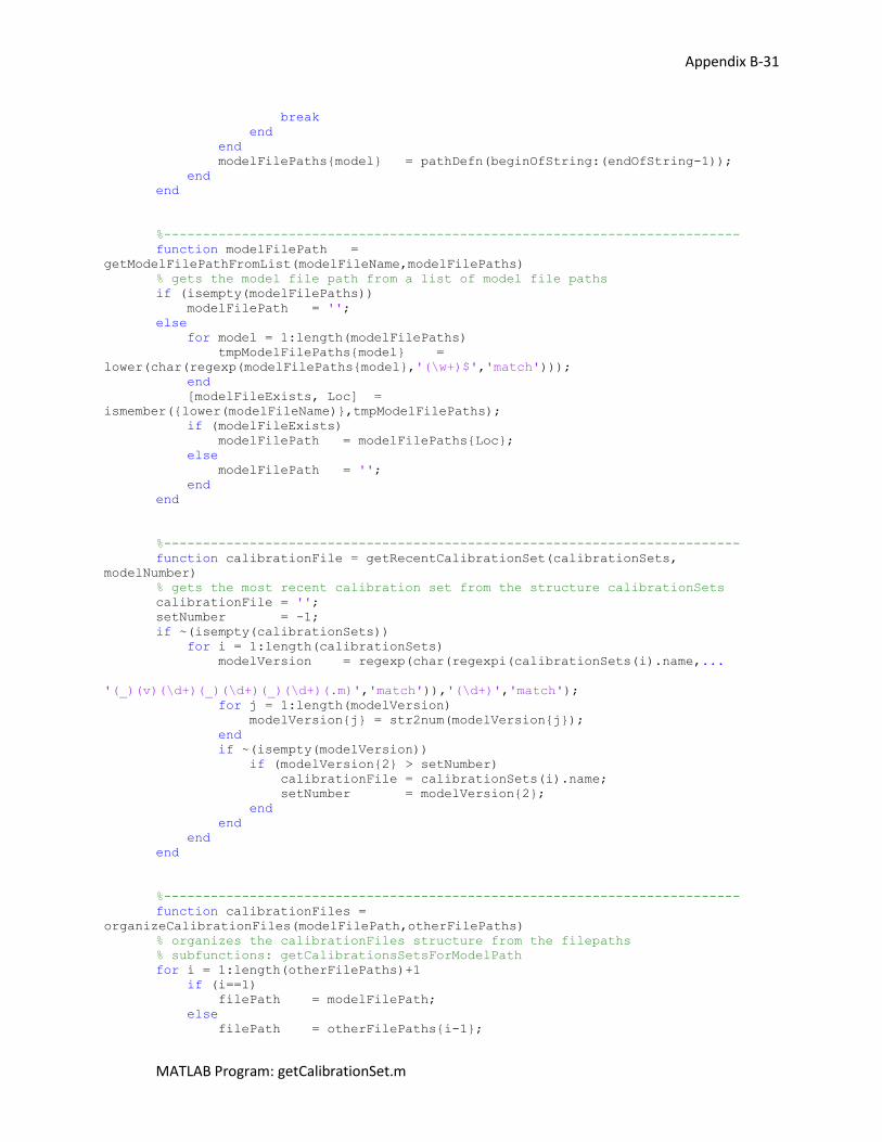
Appendix B-31
MATLAB Program: getCalibrationSet.m
break
end
end
modelFilePaths{model} = pathDefn(beginOfString:(endOfString-1));
end
end
%--------------------------------------------------------------------------
function modelFilePath =
getModelFilePathFromList(modelFileName,modelFilePaths)
% gets the model file path from a list of model file paths
if (isempty(modelFilePaths))
modelFilePath = '';
else
for model = 1:length(modelFilePaths)
tmpModelFilePaths{model} =
lower(char(regexp(modelFilePaths{model},'(\w+)$','match')));
end
[modelFileExists, Loc] =
ismember({lower(modelFileName)},tmpModelFilePaths);
if (modelFileExists)
modelFilePath = modelFilePaths{Loc};
else
modelFilePath = '';
end
end
%--------------------------------------------------------------------------
function calibrationFile = getRecentCalibrationSet(calibrationSets,
modelNumber)
% gets the most recent calibration set from the structure calibrationSets
calibrationFile = '';
setNumber = -1;
if ~(isempty(calibrationSets))
for i = 1:length(calibrationSets)
modelVersion = regexp(char(regexpi(calibrationSets(i).name,...
'(_)(v)(\d+)(_)(\d+)(_)(\d+)(.m)','match')),'(\d+)','match');
for j = 1:length(modelVersion)
modelVersion{j} = str2num(modelVersion{j});
end
if ~(isempty(modelVersion))
if (modelVersion{2} > setNumber)
calibrationFile = calibrationSets(i).name;
setNumber = modelVersion{2};
end
end
end
end
%--------------------------------------------------------------------------
function calibrationFiles =
organizeCalibrationFiles(modelFilePath,otherFilePaths)
% organizes the calibrationFiles structure from the filepaths
% subfunctions: getCalibrationsSetsForModelPath
for i = 1:length(otherFilePaths)+1
if (i==1)
filePath = modelFilePath;
else
filePath = otherFilePaths{i-1};
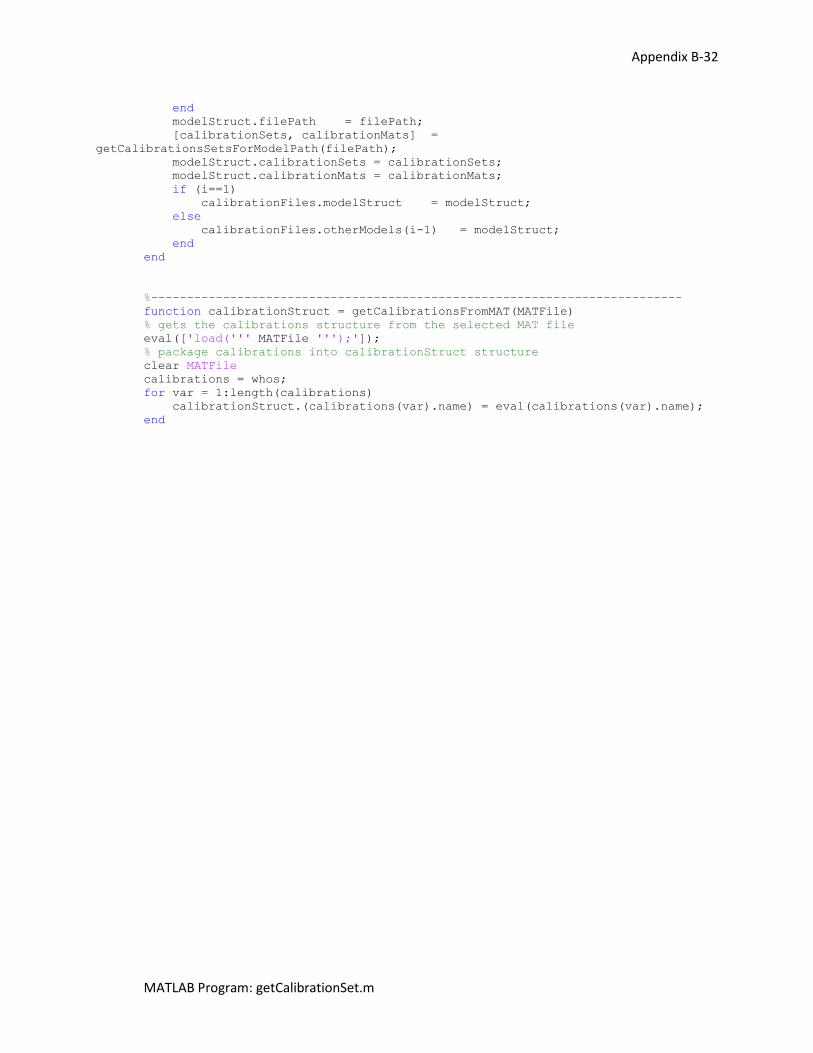
Appendix B-32
MATLAB Program: getCalibrationSet.m
end
modelStruct.filePath = filePath;
[calibrationSets, calibrationMats] =
getCalibrationsSetsForModelPath(filePath);
modelStruct.calibrationSets = calibrationSets;
modelStruct.calibrationMats = calibrationMats;
if (i==1)
calibrationFiles.modelStruct = modelStruct;
else
calibrationFiles.otherModels(i-1) = modelStruct;
end
end
%--------------------------------------------------------------------------
function calibrationStruct = getCalibrationsFromMAT(MATFile)
% gets the calibrations structure from the selected MAT file
eval(['load(''' MATFile ''');']);
% package calibrations into calibrationStruct structure
clear MATFile
calibrations = whos;
for var = 1:length(calibrations)
calibrationStruct.(calibrations(var).name) = eval(calibrations(var).name);
end
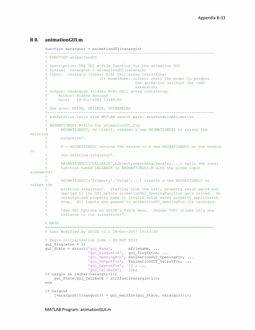
Appendix B-33
MATLAB Program: animationGUI.m
B 8. animationGUI.m
function varargout = animationGUI(varargin)
%--------------------------------------------------------------------------
% FUNCTION animationGUI
%
% Description: The GUI m-file function for the animation GUI
% Syntax: varargout = animationGUI(varargin)
% Input: varargin (class: N/A) Cell array containing:
% (1) modelName: (class: char) The model to produce
% the animation (without the .mdl
% extension)
% Output: varargout (class: N/A) Cell array containing:
% Author: Andrew Hovingh
% Date: 18-Oct-2007 13:40:50
%
% See also: GUIDE, GUIDATA, GUIHANDLES
%--------------------------------------------------------------------------
% subfunction calls from MATLAB search path: makePendulumAnimation
%
% ANIMATIONGUI M-file for animationGUI.fig
% ANIMATIONGUI, by itself, creates a new ANIMATIONGUI or raises the
existing
% singleton*.
%
% H = ANIMATIONGUI returns the handle to a new ANIMATIONGUI or the handle
to
% the existing singleton*.
%
% ANIMATIONGUI('CALLBACK',hObject,eventData,handles,...) calls the local
% function named CALLBACK in ANIMATIONGUI.M with the given input
arguments.
%
% ANIMATIONGUI('Property','Value',...) creates a new ANIMATIONGUI or
raises the
% existing singleton*. Starting from the left, property value pairs are
% applied to the GUI before animationGUI_OpeningFunction gets called. An
% unrecognized property name or invalid value makes property application
% stop. All inputs are passed to animationGUI_OpeningFcn via varargin.
%
% *See GUI Options on GUIDE's Tools menu. Choose "GUI allows only one
% instance to run (singleton)".
% MAIN
%==========================================================================
% Last Modified by GUIDE v2.5 28-Oct-2007 15:13:39
% Begin initialization code - DO NOT EDIT
gui_Singleton = 1;
gui_State = struct('gui_Name', mfilename, ...
'gui_Singleton', gui_Singleton, ...
'gui_OpeningFcn', @animationGUI_OpeningFcn, ...
'gui_OutputFcn', @animationGUI_OutputFcn, ...
'gui_LayoutFcn', [] , ...
'gui_Callback', []);
if nargin && ischar(varargin{1})
gui_State.gui_Callback = str2func(varargin{1});
end
if nargout
[varargout{1:nargout}] = gui_mainfcn(gui_State, varargin{:});
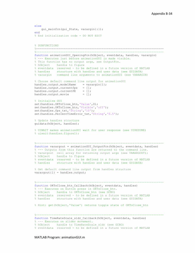
Appendix B-34
MATLAB Program: animationGUI.m
else
gui_mainfcn(gui_State, varargin{:});
end
% End initialization code - DO NOT EDIT
% SUBFUNCTIONS
%==========================================================================
%--------------------------------------------------------------------------
function animationGUI_OpeningFcn(hObject, eventdata, handles, varargin)
% --- Executes just before animationGUI is made visible.
% This function has no output args, see OutputFcn.
% hObject handle to figure
% eventdata reserved - to be defined in a future version of MATLAB
% handles structure with handles and user data (see GUIDATA)
% varargin command line arguments to animationGUI (see VARARGIN)
% Choose default command line output for animationGUI
handles.output.modelName = varargin{1};
handles.output.currentfps = [];
handles.output.currentPE = [];
handles.output.movie = [];
% Initialize GUI
set(handles.OKToClose_btn,'Value',0);
set(handles.OKToClose_btn,'Visible','off');
set(handles.fps_txt,'String','10');
set(handles.PercentTimeError_txt,'String','0.5');
% Update handles structure
guidata(hObject, handles);
% UIWAIT makes animationGUI wait for user response (see UIRESUME)
% uiwait(handles.figure1);
%--------------------------------------------------------------------------
function varargout = animationGUI_OutputFcn(hObject, eventdata, handles)
% --- Outputs from this function are returned to the command line.
% varargout cell array for returning output args (see VARARGOUT);
% hObject handle to figure
% eventdata reserved - to be defined in a future version of MATLAB
% handles structure with handles and user data (see GUIDATA)
% Get default command line output from handles structure
varargout{1} = handles.output;
%--------------------------------------------------------------------------
function OKToClose_btn_Callback(hObject, eventdata, handles)
% --- Executes on button press in OKToClose_btn.
% hObject handle to OKToClose_btn (see GCBO)
% eventdata reserved - to be defined in a future version of MATLAB
% handles structure with handles and user data (see GUIDATA)
% Hint: get(hObject,'Value') returns toggle state of OKToClose_btn
%--------------------------------------------------------------------------
function TimeRateScale_sldr_Callback(hObject, eventdata, handles)
% --- Executes on slider movement.
% hObject handle to TimeRateScale_sldr (see GCBO)
% eventdata reserved - to be defined in a future version of MATLAB
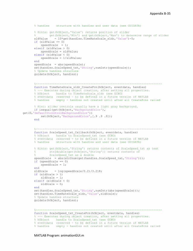
Appendix B-35
MATLAB Program: animationGUI.m
% handles structure with handles and user data (see GUIDATA)
% Hints: get(hObject,'Value') returns position of slider
% get(hObject,'Min') and get(hObject,'Max') to determine range of slider
sldValue = 10*get(handles.TimeRateScale_sldr,'Value')-5;
if (sldValue == 0)
speedScale = 1;
elseif (sldValue > 0)
speedScale = sldValue;
elseif (sldValue < 0)
speedScale = 1/sldValue;
end
speedScale = abs(speedScale);
set(handles.ScaleSpeed_txt,'String',num2str(speedScale));
% Update handles structure
guidata(hObject, handles);
%--------------------------------------------------------------------------
function TimeRateScale_sldr_CreateFcn(hObject, eventdata, handles)
% --- Executes during object creation, after setting all properties.
% hObject handle to TimeRateScale_sldr (see GCBO)
% eventdata reserved - to be defined in a future version of MATLAB
% handles empty - handles not created until after all CreateFcns called
% Hint: slider controls usually have a light gray background.
if isequal(get(hObject,'BackgroundColor'),
get(0,'defaultUicontrolBackgroundColor'))
set(hObject,'BackgroundColor',[.9 .9 .9]);
end
%--------------------------------------------------------------------------
function ScaleSpeed_txt_Callback(hObject, eventdata, handles)
% hObject handle to ScaleSpeed_txt (see GCBO)
% eventdata reserved - to be defined in a future version of MATLAB
% handles structure with handles and user data (see GUIDATA)
% Hints: get(hObject,'String') returns contents of ScaleSpeed_txt as text
% str2double(get(hObject,'String')) returns contents of
% ScaleSpeed_txt as a double
speedScale = abs(str2num(get(handles.ScaleSpeed_txt,'String')));
if (speedScale == 0)
speedScale = 1;
end
sldScale = log(speedScale/0.2)/3.218;
if (sldScale > 1)
sldScale = 1;
elseif (sldScale < 0)
sldScale = 0;
end
set(handles.ScaleSpeed_txt,'String',num2str(abs(speedScale)));
set(handles.TimeRateScale_sldr,'Value',sldScale);
% Update handles structure
guidata(hObject, handles);
%--------------------------------------------------------------------------
function ScaleSpeed_txt_CreateFcn(hObject, eventdata, handles)
% --- Executes during object creation, after setting all properties.
% hObject handle to ScaleSpeed_txt (see GCBO)
% eventdata reserved - to be defined in a future version of MATLAB
% handles empty - handles not created until after all CreateFcns called
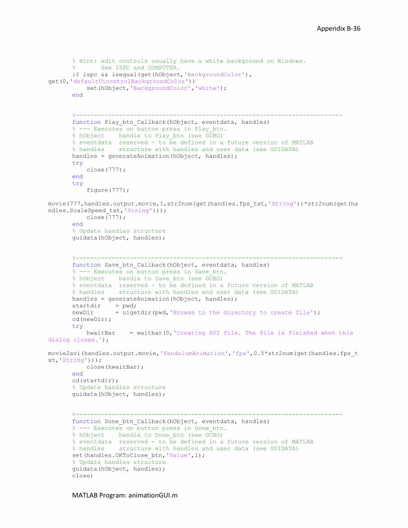
Appendix B-36
MATLAB Program: animationGUI.m
% Hint: edit controls usually have a white background on Windows.
% See ISPC and COMPUTER.
if ispc && isequal(get(hObject,'BackgroundColor'),
get(0,'defaultUicontrolBackgroundColor'))
set(hObject,'BackgroundColor','white');
end
%--------------------------------------------------------------------------
function Play_btn_Callback(hObject, eventdata, handles)
% --- Executes on button press in Play_btn.
% hObject handle to Play_btn (see GCBO)
% eventdata reserved - to be defined in a future version of MATLAB
% handles structure with handles and user data (see GUIDATA)
handles = generateAnimation(hObject, handles);
try
close(777);
end
try
figure(777);
movie(777,handles.output.movie,1,str2num(get(handles.fps_txt,'String'))*str2num(get(ha
ndles.ScaleSpeed_txt,'String')));
close(777);
end
% Update handles structure
guidata(hObject, handles);
%--------------------------------------------------------------------------
function Save_btn_Callback(hObject, eventdata, handles)
% --- Executes on button press in Save_btn.
% hObject handle to Save_btn (see GCBO)
% eventdata reserved - to be defined in a future version of MATLAB
% handles structure with handles and user data (see GUIDATA)
handles = generateAnimation(hObject, handles);
startdir = pwd;
newDir = uigetdir(pwd,'Browse to the directory to create file');
cd(newDir);
try
hwaitBar = waitbar(0,'Creating AVI file. The file is finished when this
dialog closes.');
movie2avi(handles.output.movie,'PendulumAnimation','fps',0.5*str2num(get(handles.fps_t
xt,'String')));
close(hwaitBar);
end
cd(startdir);
% Update handles structure
guidata(hObject, handles);
%--------------------------------------------------------------------------
function Done_btn_Callback(hObject, eventdata, handles)
% --- Executes on button press in Done_btn.
% hObject handle to Done_btn (see GCBO)
% eventdata reserved - to be defined in a future version of MATLAB
% handles structure with handles and user data (see GUIDATA)
set(handles.OKToClose_btn,'Value',1);
% Update handles structure
guidata(hObject, handles);
close;
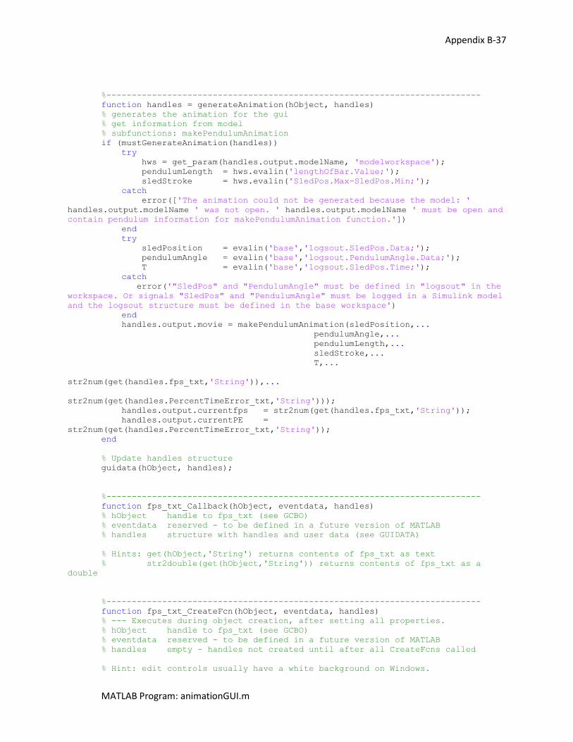
Appendix B-37
MATLAB Program: animationGUI.m
%--------------------------------------------------------------------------
function handles = generateAnimation(hObject, handles)
% generates the animation for the gui
% get information from model
% subfunctions: makePendulumAnimation
if (mustGenerateAnimation(handles))
try
hws = get_param(handles.output.modelName, 'modelworkspace');
pendulumLength = hws.evalin('lengthOfBar.Value;');
sledStroke = hws.evalin('SledPos.Max-SledPos.Min;');
catch
error(['The animation could not be generated because the model: '
handles.output.modelName ' was not open. ' handles.output.modelName ' must be open and
contain pendulum information for makePendulumAnimation function.'])
end
try
sledPosition = evalin('base','logsout.SledPos.Data;');
pendulumAngle = evalin('base','logsout.PendulumAngle.Data;');
T = evalin('base','logsout.SledPos.Time;');
catch
error('"SledPos" and "PendulumAngle" must be defined in "logsout" in the
workspace. Or signals "SledPos" and "PendulumAngle" must be logged in a Simulink model
and the logsout structure must be defined in the base workspace')
end
handles.output.movie = makePendulumAnimation(sledPosition,...
pendulumAngle,...
pendulumLength,...
sledStroke,...
T,...
str2num(get(handles.fps_txt,'String')),...
str2num(get(handles.PercentTimeError_txt,'String')));
handles.output.currentfps = str2num(get(handles.fps_txt,'String'));
handles.output.currentPE =
str2num(get(handles.PercentTimeError_txt,'String'));
end
% Update handles structure
guidata(hObject, handles);
%--------------------------------------------------------------------------
function fps_txt_Callback(hObject, eventdata, handles)
% hObject handle to fps_txt (see GCBO)
% eventdata reserved - to be defined in a future version of MATLAB
% handles structure with handles and user data (see GUIDATA)
% Hints: get(hObject,'String') returns contents of fps_txt as text
% str2double(get(hObject,'String')) returns contents of fps_txt as a
double
%--------------------------------------------------------------------------
function fps_txt_CreateFcn(hObject, eventdata, handles)
% --- Executes during object creation, after setting all properties.
% hObject handle to fps_txt (see GCBO)
% eventdata reserved - to be defined in a future version of MATLAB
% handles empty - handles not created until after all CreateFcns called
% Hint: edit controls usually have a white background on Windows.
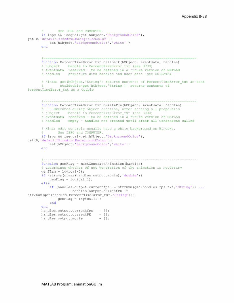
Appendix B-38
MATLAB Program: animationGUI.m
% See ISPC and COMPUTER.
if ispc && isequal(get(hObject,'BackgroundColor'),
get(0,'defaultUicontrolBackgroundColor'))
set(hObject,'BackgroundColor','white');
end
%--------------------------------------------------------------------------
function PercentTimeError_txt_Callback(hObject, eventdata, handles)
% hObject handle to PercentTimeError_txt (see GCBO)
% eventdata reserved - to be defined in a future version of MATLAB
% handles structure with handles and user data (see GUIDATA)
% Hints: get(hObject,'String') returns contents of PercentTimeError_txt as text
% str2double(get(hObject,'String')) returns contents of
PercentTimeError_txt as a double
%--------------------------------------------------------------------------
function PercentTimeError_txt_CreateFcn(hObject, eventdata, handles)
% --- Executes during object creation, after setting all properties.
% hObject handle to PercentTimeError_txt (see GCBO)
% eventdata reserved - to be defined in a future version of MATLAB
% handles empty - handles not created until after all CreateFcns called
% Hint: edit controls usually have a white background on Windows.
% See ISPC and COMPUTER.
if ispc && isequal(get(hObject,'BackgroundColor'),
get(0,'defaultUicontrolBackgroundColor'))
set(hObject,'BackgroundColor','white');
end
%--------------------------------------------------------------------------
function genFlag = mustGenerateAnimation(handles)
% determines whether of not generation of the animation is necessary
genFlag = logical(0);
if (strcmp(class(handles.output.movie),'double'))
genFlag = logical(1);
else
if (handles.output.currentfps ~= str2num(get(handles.fps_txt,'String')) ...
|| handles.output.currentPE ~=
str2num(get(handles.PercentTimeError_txt,'String')))
genFlag = logical(1);
end
end
handles.output.currentfps = [];
handles.output.currentPE = [];
handles.output.movie = [];
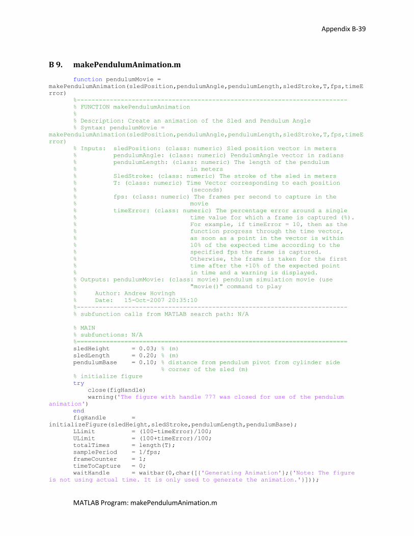
Appendix B-39
MATLAB Program: makePendulumAnimation.m
B 9. makePendulumAnimation.m
function pendulumMovie =
makePendulumAnimation(sledPosition,pendulumAngle,pendulumLength,sledStroke,T,fps,timeE
rror)
%--------------------------------------------------------------------------
% FUNCTION makePendulumAnimation
%
% Description: Create an animation of the Sled and Pendulum Angle
% Syntax: pendulumMovie =
makePendulumAnimation(sledPosition,pendulumAngle,pendulumLength,sledStroke,T,fps,timeE
rror)
% Inputs: sledPosition: (class: numeric) Sled position vector in meters
% pendulumAngle: (class: numeric) PendulumAngle vector in radians
% pendulumLength: (class: numeric) The length of the pendulum
% in meters
% SledStroke: (class: numeric) The stroke of the sled in meters
% T: (class: numeric) Time Vector corresponding to each position
% (seconds)
% fps: (class: numeric) The frames per second to capture in the
% movie
% timeError: (class: numeric) The percentage error around a single
% time value for which a frame is captured (%).
% For example, if timeError = 10, then as the
% function progress through the time vector,
% as soon as a point in the vector is within
% 10% of the expected time according to the
% specified fps the frame is captured.
% Otherwise, the frame is taken for the first
% time after the +10% of the expected point
% in time and a warning is displayed.
% Outputs: pendulumMovie: (class: movie) pendulum simulation movie (use
% "movie()" command to play
% Author: Andrew Hovingh
% Date: 15-Oct-2007 20:35:10
%--------------------------------------------------------------------------
% subfunction calls from MATLAB search path: N/A
% MAIN
% subfunctions: N/A
%==========================================================================
sledHeight = 0.03; % (m)
sledLength = 0.20; % (m)
pendulumBase = 0.10; % distance from pendulum pivot from cylinder side
% corner of the sled (m)
% initialize figure
try
close(figHandle)
warning('The figure with handle 777 was closed for use of the pendulum
animation')
end
figHandle =
initializeFigure(sledHeight,sledStroke,pendulumLength,pendulumBase);
LLimit = (100-timeError)/100;
ULimit = (100+timeError)/100;
totalTimes = length(T);
samplePeriod = 1/fps;
frameCounter = 1;
timeToCapture = 0;
waitHandle = waitbar(0,char([{'Generating Animation'};{'Note: The figure
is not using actual time. It is only used to generate the animation.'}]));
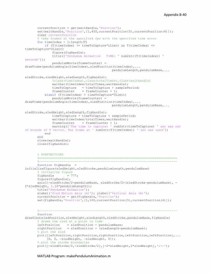
Appendix B-40
MATLAB Program: makePendulumAnimation.m
currentPosition = get(waitHandle,'Position');
set(waitHandle,'Position',[1,450,currentPosition(3),currentPosition(4)]);
clear currentPosition
% take frames at the specified fps with the specified time error
for timeIndex = 1:length(T)
if (T(timeIndex) >= timeToCapture*LLimit && T(timeIndex) <=
timeToCapture*ULimit)
figure(figHandle);
title(['Pendumum Animation TIME: ' num2str(T(timeIndex)) '
seconds']);
pendulumMovie(frameCounter) =
drawFrame(pendulumAngle(timeIndex),sledPosition(timeIndex),...
pendulumLength,pendulumBase,...
sledStroke,sledHeight,sledLength,figHandle);
%class(timeIndex),class(totalTimes),class(waitHandle)
waitbar(timeIndex/totalTimes,waitHandle);
timeToCapture = timeToCapture + samplePeriod;
frameCounter = frameCounter + 1;
elseif (T(timeIndex) > timeToCapture*ULimit)
pendulumMovie(frameCounter) =
drawFrame(pendulumAngle(timeIndex),sledPosition(timeIndex),...
pendulumLength,pendulumBase,...
sledStroke,sledHeight,sledLength,figHandle);
timeToCapture = timeToCapture + samplePeriod;
waitbar(timeIndex/totalTimes,waitHandle);
frameCounter = frameCounter + 1;
warning(['The time to capture: ' num2str(timeToCapture) ' sec was out
of bounds of T vector. The frame at ' num2str(T(timeIndex)) ' sec was used'])
end
end
close(waitHandle);
close(figHandle);
% SUBFUNCTIONS
%==========================================================================
%--------------------------------------------------------------------------
function figHandle =
initializeFigure(sledHeight,sledStroke,pendulumLength,pendulumBase)
% initialize figure
figHandle = 777;
figure(figHandle);
axis([-sledStroke/2-pendulumBase, sledStroke/2+(sledStroke-pendulumBase), -
2*sledHeight, 1.10*pendulumLength]);
title('Pendumum Animation');
xlabel('Sled Motion Axis (m)'); ylabel('Vertical Axis (m)');
currentPosition = get(figHandle,'Position');
set(figHandle,'Position',[1,100,currentPosition(3),currentPosition(4)]);
%--------------------------------------------------------------------------
function
drawSled(sledPosition,sledHeight,sledLength,sledStroke,pendulumBase,figHandle)
% draws the sled at a point in time
leftPosition = sledPosition - pendulumBase;
rightPosition = sledPosition + (sledLength-pendulumBase);
% plot the sled
plot([leftPosition,rightPosition,rightPosition,leftPosition,leftPosition],...
[0, 0, -sledHeight, -sledHeight, 0]);
% plot the stroke boundaries
plot([-sledStroke/2,-sledStroke/2],[-2*sledHeight,2*sledHeight],'r--');
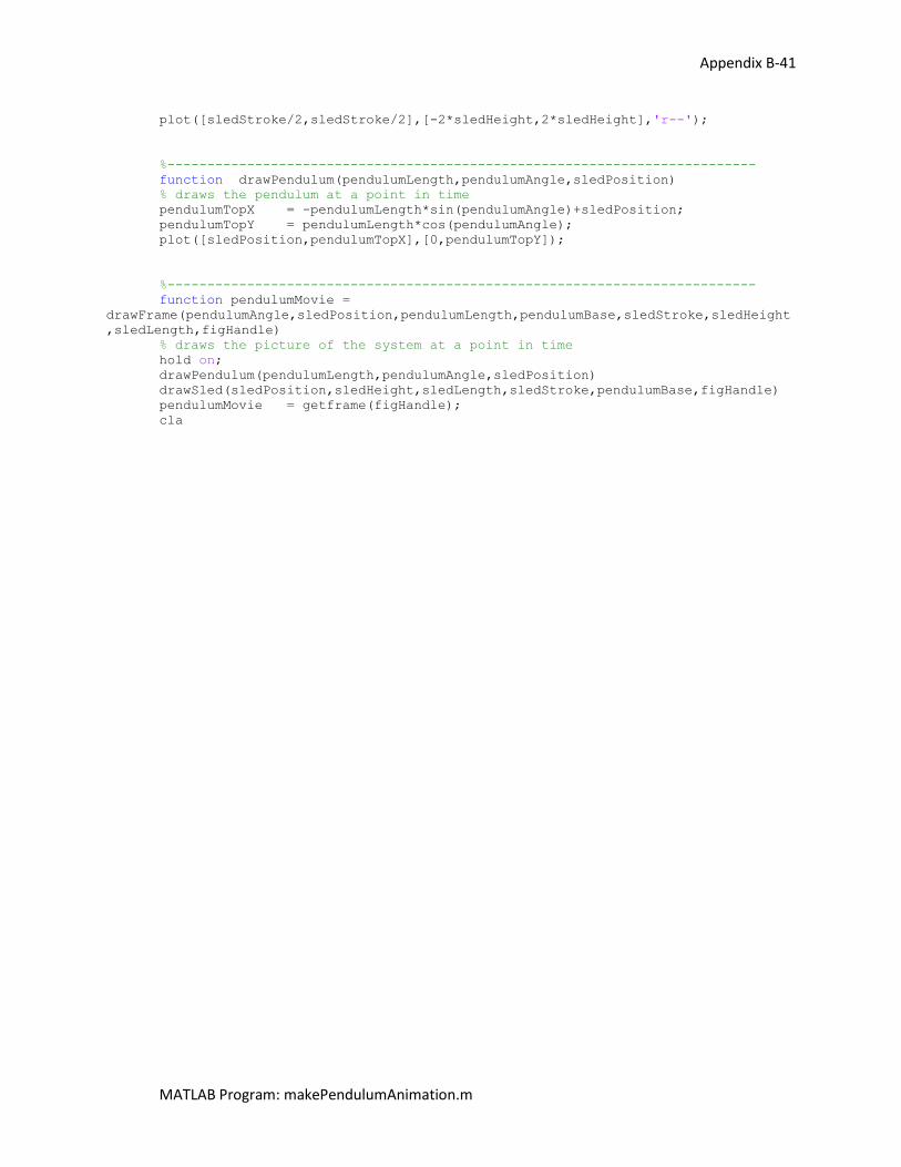
Appendix B-41
MATLAB Program: makePendulumAnimation.m
plot([sledStroke/2,sledStroke/2],[-2*sledHeight,2*sledHeight],'r--');
%--------------------------------------------------------------------------
function drawPendulum(pendulumLength,pendulumAngle,sledPosition)
% draws the pendulum at a point in time
pendulumTopX = -pendulumLength*sin(pendulumAngle)+sledPosition;
pendulumTopY = pendulumLength*cos(pendulumAngle);
plot([sledPosition,pendulumTopX],[0,pendulumTopY]);
%--------------------------------------------------------------------------
function pendulumMovie =
drawFrame(pendulumAngle,sledPosition,pendulumLength,pendulumBase,sledStroke,sledHeight
,sledLength,figHandle)
% draws the picture of the system at a point in time
hold on;
drawPendulum(pendulumLength,pendulumAngle,sledPosition)
drawSled(sledPosition,sledHeight,sledLength,sledStroke,pendulumBase,figHandle)
pendulumMovie = getframe(figHandle);
cla
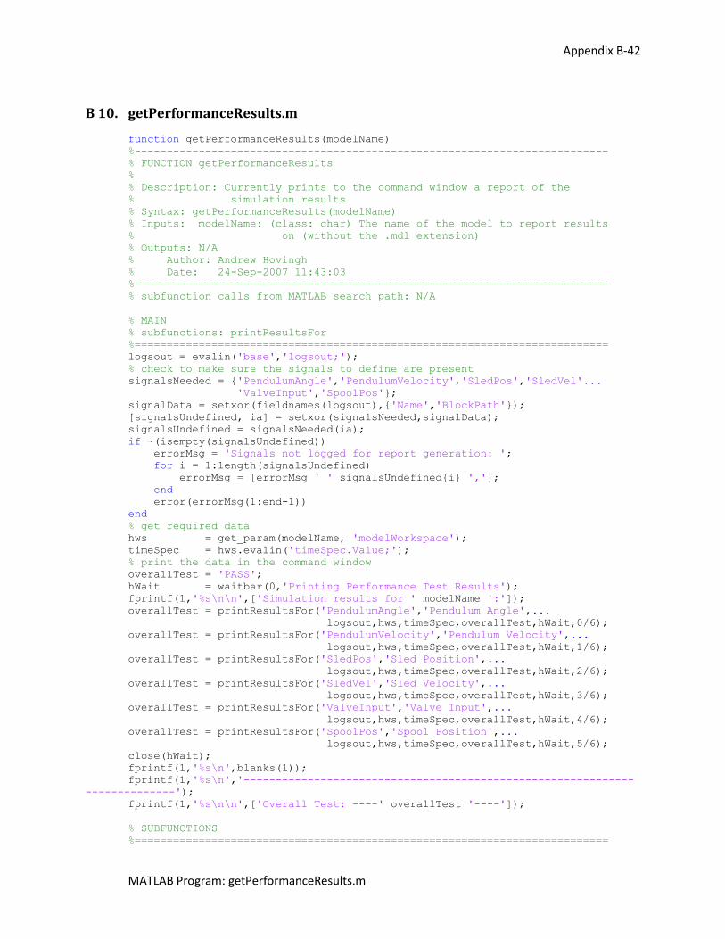
Appendix B-42
MATLAB Program: getPerformanceResults.m
B 10. getPerformanceResults.m
function getPerformanceResults(modelName)
%--------------------------------------------------------------------------
% FUNCTION getPerformanceResults
%
% Description: Currently prints to the command window a report of the
% simulation results
% Syntax: getPerformanceResults(modelName)
% Inputs: modelName: (class: char) The name of the model to report results
% on (without the .mdl extension)
% Outputs: N/A
% Author: Andrew Hovingh
% Date: 24-Sep-2007 11:43:03
%--------------------------------------------------------------------------
% subfunction calls from MATLAB search path: N/A
% MAIN
% subfunctions: printResultsFor
%==========================================================================
logsout = evalin('base','logsout;');
% check to make sure the signals to define are present
signalsNeeded = {'PendulumAngle','PendulumVelocity','SledPos','SledVel'...
'ValveInput','SpoolPos'};
signalData = setxor(fieldnames(logsout),{'Name','BlockPath'});
[signalsUndefined, ia] = setxor(signalsNeeded,signalData);
signalsUndefined = signalsNeeded(ia);
if ~(isempty(signalsUndefined))
errorMsg = 'Signals not logged for report generation: ';
for i = 1:length(signalsUndefined)
errorMsg = [errorMsg ' ' signalsUndefined{i} ','];
end
error(errorMsg(1:end-1))
end
% get required data
hws = get_param(modelName, 'modelWorkspace');
timeSpec = hws.evalin('timeSpec.Value;');
% print the data in the command window
overallTest = 'PASS';
hWait = waitbar(0,'Printing Performance Test Results');
fprintf(1,'%s\n\n',['Simulation results for ' modelName ':']);
overallTest = printResultsFor('PendulumAngle','Pendulum Angle',...
logsout,hws,timeSpec,overallTest,hWait,0/6);
overallTest = printResultsFor('PendulumVelocity','Pendulum Velocity',...
logsout,hws,timeSpec,overallTest,hWait,1/6);
overallTest = printResultsFor('SledPos','Sled Position',...
logsout,hws,timeSpec,overallTest,hWait,2/6);
overallTest = printResultsFor('SledVel','Sled Velocity',...
logsout,hws,timeSpec,overallTest,hWait,3/6);
overallTest = printResultsFor('ValveInput','Valve Input',...
logsout,hws,timeSpec,overallTest,hWait,4/6);
overallTest = printResultsFor('SpoolPos','Spool Position',...
logsout,hws,timeSpec,overallTest,hWait,5/6);
close(hWait);
fprintf(1,'%s\n',blanks(1));
fprintf(1,'%s\n','-------------------------------------------------------------
--------------');
fprintf(1,'%s\n\n',['Overall Test: ----' overallTest '----']);
% SUBFUNCTIONS
%==========================================================================
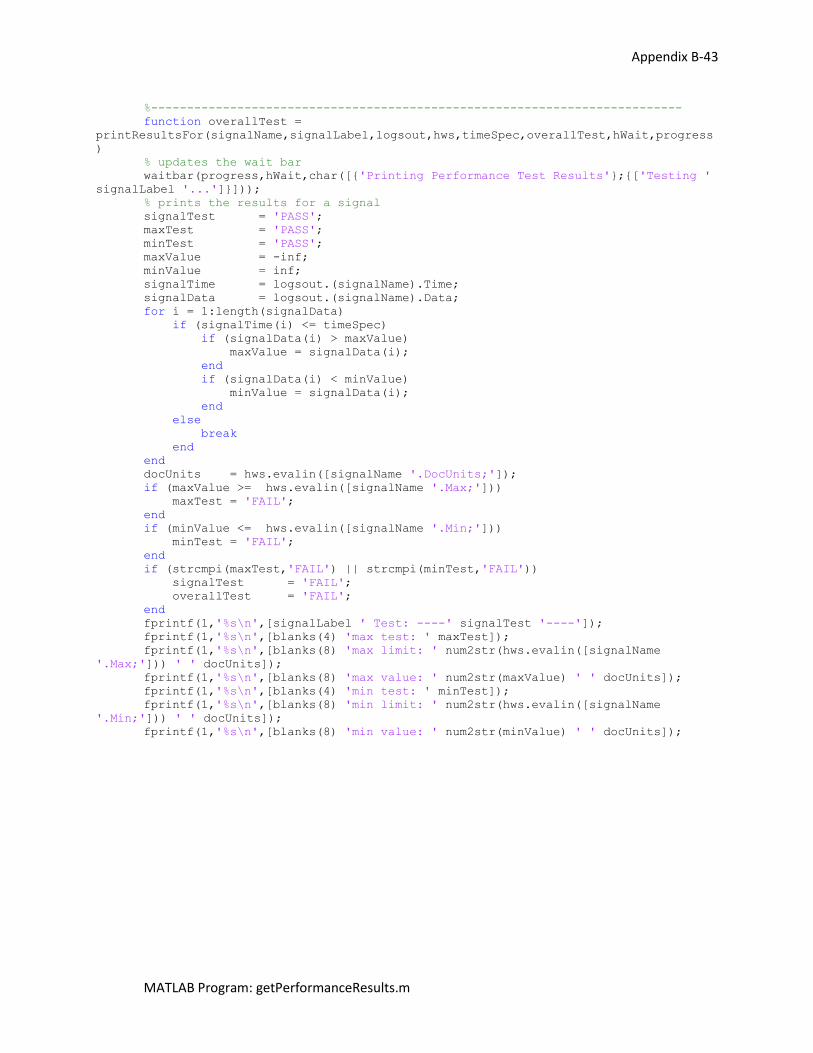
Appendix B-43
MATLAB Program: getPerformanceResults.m
%--------------------------------------------------------------------------
function overallTest =
printResultsFor(signalName,signalLabel,logsout,hws,timeSpec,overallTest,hWait,progress
)
% updates the wait bar
waitbar(progress,hWait,char([{'Printing Performance Test Results'};{['Testing '
signalLabel '...']}]));
% prints the results for a signal
signalTest = 'PASS';
maxTest = 'PASS';
minTest = 'PASS';
maxValue = -inf;
minValue = inf;
signalTime = logsout.(signalName).Time;
signalData = logsout.(signalName).Data;
for i = 1:length(signalData)
if (signalTime(i) <= timeSpec)
if (signalData(i) > maxValue)
maxValue = signalData(i);
end
if (signalData(i) < minValue)
minValue = signalData(i);
end
else
break
end
end
docUnits = hws.evalin([signalName '.DocUnits;']);
if (maxValue >= hws.evalin([signalName '.Max;']))
maxTest = 'FAIL';
end
if (minValue <= hws.evalin([signalName '.Min;']))
minTest = 'FAIL';
end
if (strcmpi(maxTest,'FAIL') || strcmpi(minTest,'FAIL'))
signalTest = 'FAIL';
overallTest = 'FAIL';
end
fprintf(1,'%s\n',[signalLabel ' Test: ----' signalTest '----']);
fprintf(1,'%s\n',[blanks(4) 'max test: ' maxTest]);
fprintf(1,'%s\n',[blanks(8) 'max limit: ' num2str(hws.evalin([signalName
'.Max;'])) ' ' docUnits]);
fprintf(1,'%s\n',[blanks(8) 'max value: ' num2str(maxValue) ' ' docUnits]);
fprintf(1,'%s\n',[blanks(4) 'min test: ' minTest]);
fprintf(1,'%s\n',[blanks(8) 'min limit: ' num2str(hws.evalin([signalName
'.Min;'])) ' ' docUnits]);
fprintf(1,'%s\n',[blanks(8) 'min value: ' num2str(minValue) ' ' docUnits]);
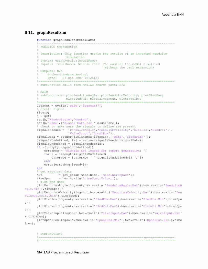
Appendix B-44
MATLAB Program: graphResults.m
B 11. graphResults.m
function graphResults(modelName)
%--------------------------------------------------------------------------
% FUNCTION tmpFunction
%
% Description: This function graphs the results of an inverted pendulum
% simulation
% Syntax: graphResults(modelName)
% Inputs: modelName: (class: char) The name of the model simulated
% (without the .mdl extension)
% Outputs: N/A
% Author: Andrew Hovingh
% Date: 23-Sep-2007 15:26:53
%--------------------------------------------------------------------------
% subfunction calls from MATLAB search path: N/A
% MAIN
% subfunctions: plotPendulumAngle, plotPendulumVelocity, plotSledPos,
% plotSledVel, plotValveInput, plotSpoolPos
%==========================================================================
logsout = evalin('base','logsout;');
% create figure
figure;
h = gcf;
set(h,'WindowStyle','docked');
set(h,'Name',['Signal Data for ' modelName]);
% check to make sure the signals to define are present
signalsNeeded = {'PendulumAngle','PendulumVelocity','SledPos','SledVel'...
'ValveInput','SpoolPos'};
signalData = setxor(fieldnames(logsout),{'Name','BlockPath'});
[signalsUndefined, ia] = setxor(signalsNeeded,signalData);
signalsUndefined = signalsNeeded(ia);
if ~(isempty(signalsUndefined))
errorMsg = 'Signals not logged for report generation: ';
for i = 1:length(signalsUndefined)
errorMsg = [errorMsg ' ' signalsUndefined{i} ','];
end
error(errorMsg(1:end-1))
end
% get required data
hws = get_param(modelName, 'modelWorkspace');
timeSpec = hws.evalin('timeSpec.Value;');
% plot the data
plotPendulumAngle(logsout,hws.evalin('PendulumAngle.Max'),hws.evalin('PendulumA
ngle.Min'),timeSpec);
plotPendulumVelocity(logsout,hws.evalin('PendulumVelocity.Max'),hws.evalin('Pen
dulumVelocity.Min'),timeSpec);
plotSledPos(logsout,hws.evalin('SledPos.Max'),hws.evalin('SledPos.Min'),timeSpe
c);
plotSledVel(logsout,hws.evalin('SledVel.Max'),hws.evalin('SledVel.Min'),timeSpe
c);
plotValveInput(logsout,hws.evalin('ValveInput.Max'),hws.evalin('ValveInput.Min'
),timeSpec);
plotSpoolPos(logsout,hws.evalin('SpoolPos.Max'),hws.evalin('SpoolPos.Min'),time
Spec);
% SUBFUNCTIONS
%==========================================================================
%--------------------------------------------------------------------------
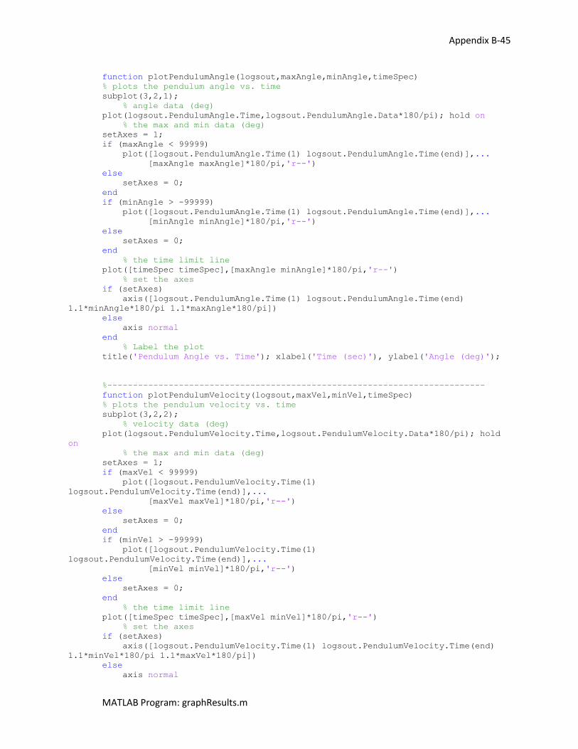
Appendix B-45
MATLAB Program: graphResults.m
function plotPendulumAngle(logsout,maxAngle,minAngle,timeSpec)
% plots the pendulum angle vs. time
subplot(3,2,1);
% angle data (deg)
plot(logsout.PendulumAngle.Time,logsout.PendulumAngle.Data*180/pi); hold on
% the max and min data (deg)
setAxes = 1;
if (maxAngle < 99999)
plot([logsout.PendulumAngle.Time(1) logsout.PendulumAngle.Time(end)],...
[maxAngle maxAngle]*180/pi,'r--')
else
setAxes = 0;
end
if (minAngle > -99999)
plot([logsout.PendulumAngle.Time(1) logsout.PendulumAngle.Time(end)],...
[minAngle minAngle]*180/pi,'r--')
else
setAxes = 0;
end
% the time limit line
plot([timeSpec timeSpec],[maxAngle minAngle]*180/pi,'r--')
% set the axes
if (setAxes)
axis([logsout.PendulumAngle.Time(1) logsout.PendulumAngle.Time(end)
1.1*minAngle*180/pi 1.1*maxAngle*180/pi])
else
axis normal
end
% Label the plot
title('Pendulum Angle vs. Time'); xlabel('Time (sec)'), ylabel('Angle (deg)');
%--------------------------------------------------------------------------
function plotPendulumVelocity(logsout,maxVel,minVel,timeSpec)
% plots the pendulum velocity vs. time
subplot(3,2,2);
% velocity data (deg)
plot(logsout.PendulumVelocity.Time,logsout.PendulumVelocity.Data*180/pi); hold
on
% the max and min data (deg)
setAxes = 1;
if (maxVel < 99999)
plot([logsout.PendulumVelocity.Time(1)
logsout.PendulumVelocity.Time(end)],...
[maxVel maxVel]*180/pi,'r--')
else
setAxes = 0;
end
if (minVel > -99999)
plot([logsout.PendulumVelocity.Time(1)
logsout.PendulumVelocity.Time(end)],...
[minVel minVel]*180/pi,'r--')
else
setAxes = 0;
end
% the time limit line
plot([timeSpec timeSpec],[maxVel minVel]*180/pi,'r--')
% set the axes
if (setAxes)
axis([logsout.PendulumVelocity.Time(1) logsout.PendulumVelocity.Time(end)
1.1*minVel*180/pi 1.1*maxVel*180/pi])
else
axis normal
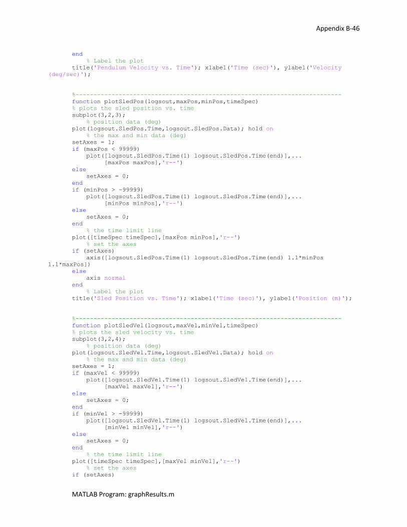
Appendix B-46
MATLAB Program: graphResults.m
end
% Label the plot
title('Pendulum Velocity vs. Time'); xlabel('Time (sec)'), ylabel('Velocity
(deg/sec)');
%--------------------------------------------------------------------------
function plotSledPos(logsout,maxPos,minPos,timeSpec)
% plots the sled position vs. time
subplot(3,2,3);
% position data (deg)
plot(logsout.SledPos.Time,logsout.SledPos.Data); hold on
% the max and min data (deg)
setAxes = 1;
if (maxPos < 99999)
plot([logsout.SledPos.Time(1) logsout.SledPos.Time(end)],...
[maxPos maxPos],'r--')
else
setAxes = 0;
end
if (minPos > -99999)
plot([logsout.SledPos.Time(1) logsout.SledPos.Time(end)],...
[minPos minPos],'r--')
else
setAxes = 0;
end
% the time limit line
plot([timeSpec timeSpec],[maxPos minPos],'r--')
% set the axes
if (setAxes)
axis([logsout.SledPos.Time(1) logsout.SledPos.Time(end) 1.1*minPos
1.1*maxPos])
else
axis normal
end
% Label the plot
title('Sled Position vs. Time'); xlabel('Time (sec)'), ylabel('Position (m)');
%--------------------------------------------------------------------------
function plotSledVel(logsout,maxVel,minVel,timeSpec)
% plots the sled velocity vs. time
subplot(3,2,4);
% position data (deg)
plot(logsout.SledVel.Time,logsout.SledVel.Data); hold on
% the max and min data (deg)
setAxes = 1;
if (maxVel < 99999)
plot([logsout.SledVel.Time(1) logsout.SledVel.Time(end)],...
[maxVel maxVel],'r--')
else
setAxes = 0;
end
if (minVel > -99999)
plot([logsout.SledVel.Time(1) logsout.SledVel.Time(end)],...
[minVel minVel],'r--')
else
setAxes = 0;
end
% the time limit line
plot([timeSpec timeSpec],[maxVel minVel],'r--')
% set the axes
if (setAxes)
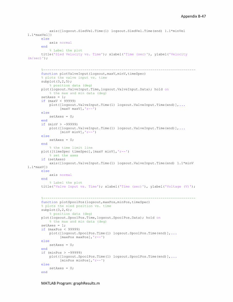
Appendix B-47
MATLAB Program: graphResults.m
axis([logsout.SledVel.Time(1) logsout.SledVel.Time(end) 1.1*minVel
1.1*maxVel])
else
axis normal
end
% Label the plot
title('Sled Velocity vs. Time'); xlabel('Time (sec)'), ylabel('Velocity
(m/sec)');
%--------------------------------------------------------------------------
function plotValveInput(logsout,maxV,minV,timeSpec)
% plots the valve input vs. time
subplot(3,2,5);
% position data (deg)
plot(logsout.ValveInput.Time,logsout.ValveInput.Data); hold on
% the max and min data (deg)
setAxes = 1;
if (maxV < 99999)
plot([logsout.ValveInput.Time(1) logsout.ValveInput.Time(end)],...
[maxV maxV],'r--')
else
setAxes = 0;
end
if (minV > -99999)
plot([logsout.ValveInput.Time(1) logsout.ValveInput.Time(end)],...
[minV minV],'r--')
else
setAxes = 0;
end
% the time limit line
plot([timeSpec timeSpec],[maxV minV],'r--')
% set the axes
if (setAxes)
axis([logsout.ValveInput.Time(1) logsout.ValveInput.Time(end) 1.1*minV
1.1*maxV])
else
axis normal
end
% Label the plot
title('Valve Input vs. Time'); xlabel('Time (sec)'), ylabel('Voltage (V)');
%--------------------------------------------------------------------------
function plotSpoolPos(logsout,maxPos,minPos,timeSpec)
% plots the sled position vs. time
subplot(3,2,6);
% position data (deg)
plot(logsout.SpoolPos.Time,logsout.SpoolPos.Data); hold on
% the max and min data (deg)
setAxes = 1;
if (maxPos < 99999)
plot([logsout.SpoolPos.Time(1) logsout.SpoolPos.Time(end)],...
[maxPos maxPos],'r--')
else
setAxes = 0;
end
if (minPos > -99999)
plot([logsout.SpoolPos.Time(1) logsout.SpoolPos.Time(end)],...
[minPos minPos],'r--')
else
setAxes = 0;
end
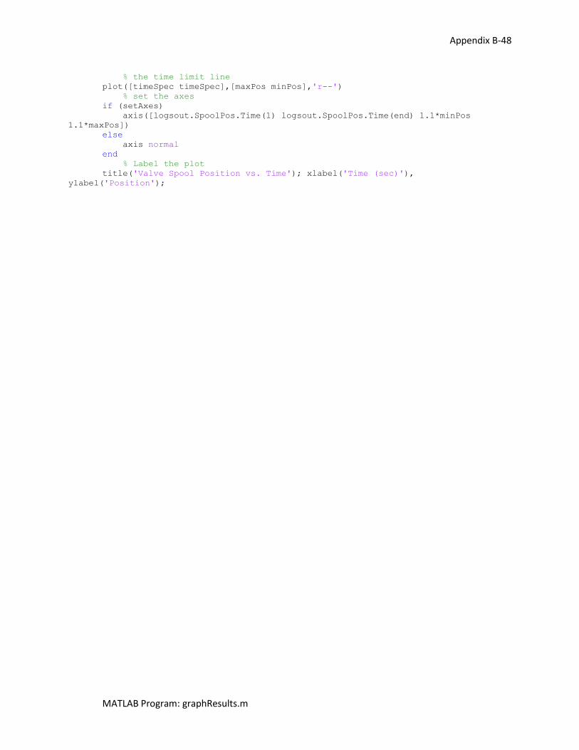
Appendix B-48
MATLAB Program: graphResults.m
% the time limit line
plot([timeSpec timeSpec],[maxPos minPos],'r--')
% set the axes
if (setAxes)
axis([logsout.SpoolPos.Time(1) logsout.SpoolPos.Time(end) 1.1*minPos
1.1*maxPos])
else
axis normal
end
% Label the plot
title('Valve Spool Position vs. Time'); xlabel('Time (sec)'),
ylabel('Position');
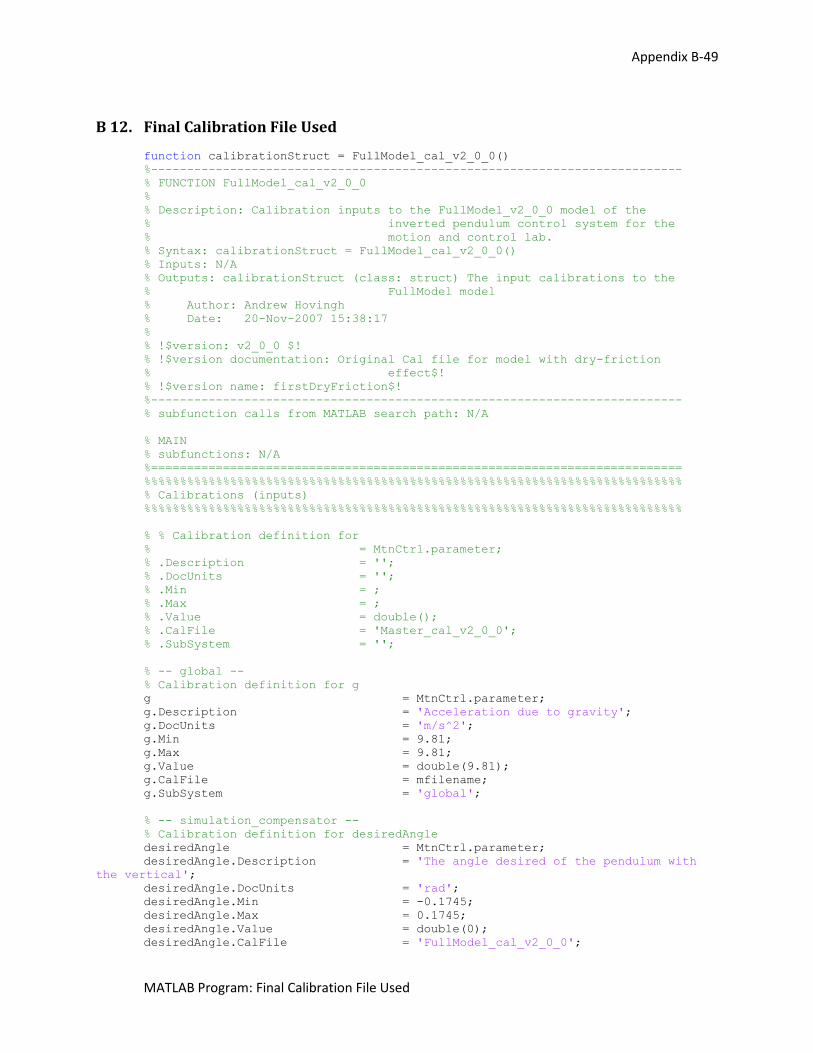
Appendix B-49
MATLAB Program: Final Calibration File Used
B 12. Final Calibration File Used
function calibrationStruct = FullModel_cal_v2_0_0()
%--------------------------------------------------------------------------
% FUNCTION FullModel_cal_v2_0_0
%
% Description: Calibration inputs to the FullModel_v2_0_0 model of the
% inverted pendulum control system for the
% motion and control lab.
% Syntax: calibrationStruct = FullModel_cal_v2_0_0()
% Inputs: N/A
% Outputs: calibrationStruct (class: struct) The input calibrations to the
% FullModel model
% Author: Andrew Hovingh
% Date: 20-Nov-2007 15:38:17
%
% !$version: v2_0_0 $!
% !$version documentation: Original Cal file for model with dry-friction
% effect$!
% !$version name: firstDryFriction$!
%--------------------------------------------------------------------------
% subfunction calls from MATLAB search path: N/A
% MAIN
% subfunctions: N/A
%==========================================================================
%%%%%%%%%%%%%%%%%%%%%%%%%%%%%%%%%%%%%%%%%%%%%%%%%%%%%%%%%%%%%%%%%%%%%%%%%%%
% Calibrations (inputs)
%%%%%%%%%%%%%%%%%%%%%%%%%%%%%%%%%%%%%%%%%%%%%%%%%%%%%%%%%%%%%%%%%%%%%%%%%%%
% % Calibration definition for
% = MtnCtrl.parameter;
% .Description = '';
% .DocUnits = '';
% .Min = ;
% .Max = ;
% .Value = double();
% .CalFile = 'Master_cal_v2_0_0';
% .SubSystem = '';
% -- global --
% Calibration definition for g
g = MtnCtrl.parameter;
g.Description = 'Acceleration due to gravity';
g.DocUnits = 'm/s^2';
g.Min = 9.81;
g.Max = 9.81;
g.Value = double(9.81);
g.CalFile = mfilename;
g.SubSystem = 'global';
% -- simulation_compensator --
% Calibration definition for desiredAngle
desiredAngle = MtnCtrl.parameter;
desiredAngle.Description = 'The angle desired of the pendulum with
the vertical';
desiredAngle.DocUnits = 'rad';
desiredAngle.Min = -0.1745;
desiredAngle.Max = 0.1745;
desiredAngle.Value = double(0);
desiredAngle.CalFile = 'FullModel_cal_v2_0_0';
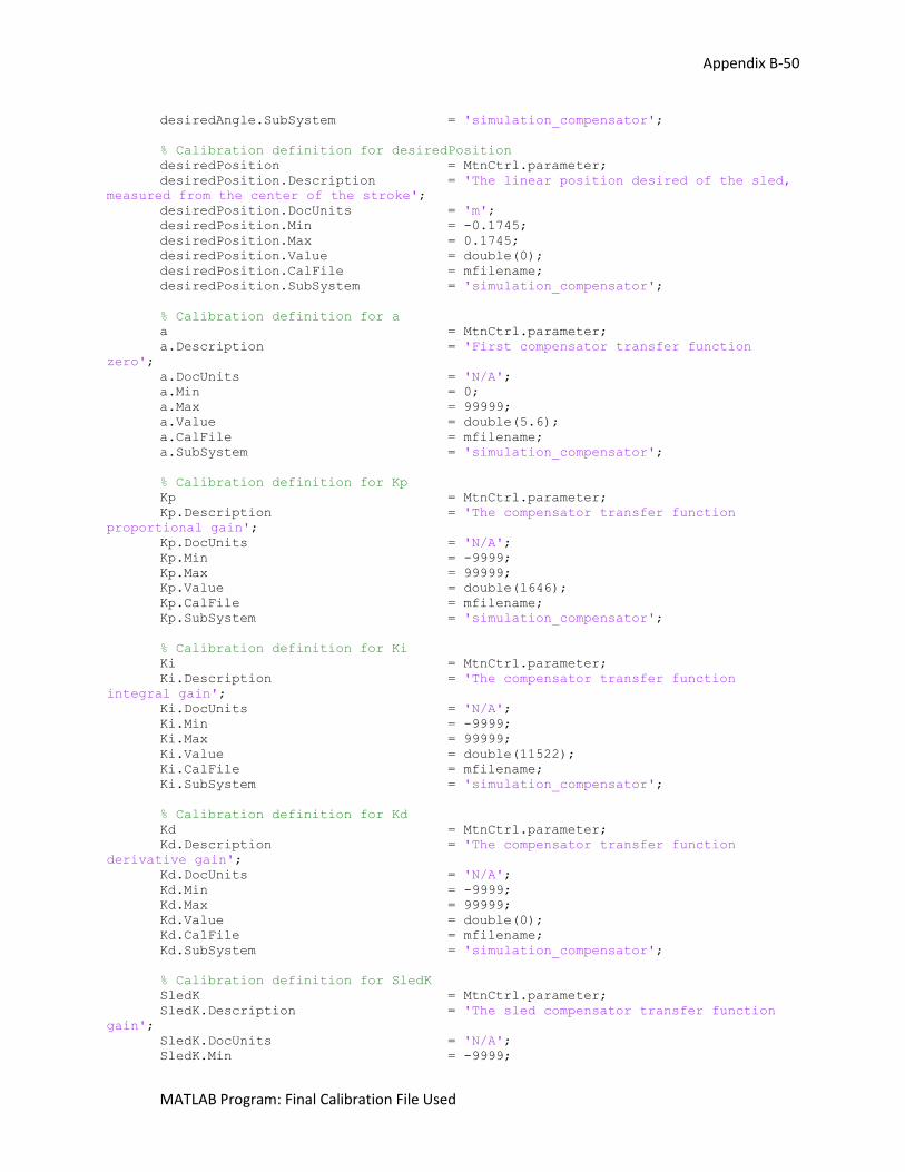
Appendix B-50
MATLAB Program: Final Calibration File Used
desiredAngle.SubSystem = 'simulation_compensator';
% Calibration definition for desiredPosition
desiredPosition = MtnCtrl.parameter;
desiredPosition.Description = 'The linear position desired of the sled,
measured from the center of the stroke';
desiredPosition.DocUnits = 'm';
desiredPosition.Min = -0.1745;
desiredPosition.Max = 0.1745;
desiredPosition.Value = double(0);
desiredPosition.CalFile = mfilename;
desiredPosition.SubSystem = 'simulation_compensator';
% Calibration definition for a
a = MtnCtrl.parameter;
a.Description = 'First compensator transfer function
zero';
a.DocUnits = 'N/A';
a.Min = 0;
a.Max = 99999;
a.Value = double(5.6);
a.CalFile = mfilename;
a.SubSystem = 'simulation_compensator';
% Calibration definition for Kp
Kp = MtnCtrl.parameter;
Kp.Description = 'The compensator transfer function
proportional gain';
Kp.DocUnits = 'N/A';
Kp.Min = -9999;
Kp.Max = 99999;
Kp.Value = double(1646);
Kp.CalFile = mfilename;
Kp.SubSystem = 'simulation_compensator';
% Calibration definition for Ki
Ki = MtnCtrl.parameter;
Ki.Description = 'The compensator transfer function
integral gain';
Ki.DocUnits = 'N/A';
Ki.Min = -9999;
Ki.Max = 99999;
Ki.Value = double(11522);
Ki.CalFile = mfilename;
Ki.SubSystem = 'simulation_compensator';
% Calibration definition for Kd
Kd = MtnCtrl.parameter;
Kd.Description = 'The compensator transfer function
derivative gain';
Kd.DocUnits = 'N/A';
Kd.Min = -9999;
Kd.Max = 99999;
Kd.Value = double(0);
Kd.CalFile = mfilename;
Kd.SubSystem = 'simulation_compensator';
% Calibration definition for SledK
SledK = MtnCtrl.parameter;
SledK.Description = 'The sled compensator transfer function
gain';
SledK.DocUnits = 'N/A';
SledK.Min = -9999;
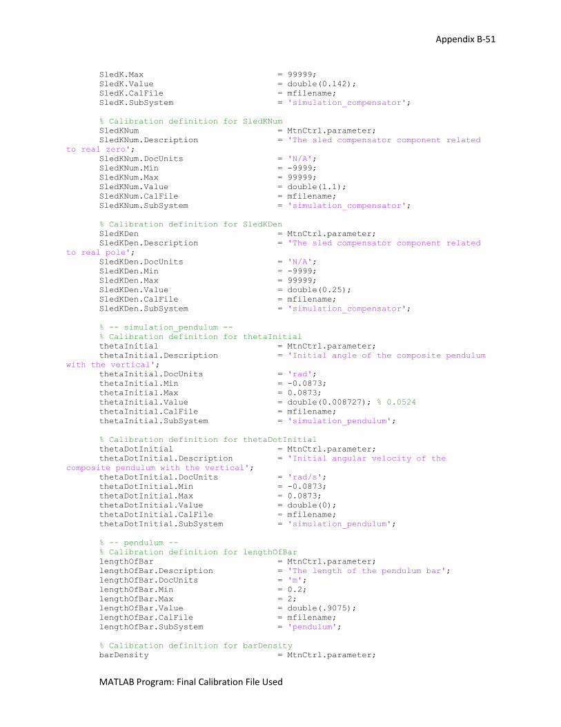
Appendix B-51
MATLAB Program: Final Calibration File Used
SledK.Max = 99999;
SledK.Value = double(0.142);
SledK.CalFile = mfilename;
SledK.SubSystem = 'simulation_compensator';
% Calibration definition for SledKNum
SledKNum = MtnCtrl.parameter;
SledKNum.Description = 'The sled compensator component related
to real zero';
SledKNum.DocUnits = 'N/A';
SledKNum.Min = -9999;
SledKNum.Max = 99999;
SledKNum.Value = double(1.1);
SledKNum.CalFile = mfilename;
SledKNum.SubSystem = 'simulation_compensator';
% Calibration definition for SledKDen
SledKDen = MtnCtrl.parameter;
SledKDen.Description = 'The sled compensator component related
to real pole';
SledKDen.DocUnits = 'N/A';
SledKDen.Min = -9999;
SledKDen.Max = 99999;
SledKDen.Value = double(0.25);
SledKDen.CalFile = mfilename;
SledKDen.SubSystem = 'simulation_compensator';
% -- simulation_pendulum --
% Calibration definition for thetaInitial
thetaInitial = MtnCtrl.parameter;
thetaInitial.Description = 'Initial angle of the composite pendulum
with the vertical';
thetaInitial.DocUnits = 'rad';
thetaInitial.Min = -0.0873;
thetaInitial.Max = 0.0873;
thetaInitial.Value = double(0.008727); % 0.0524
thetaInitial.CalFile = mfilename;
thetaInitial.SubSystem = 'simulation_pendulum';
% Calibration definition for thetaDotInitial
thetaDotInitial = MtnCtrl.parameter;
thetaDotInitial.Description = 'Initial angular velocity of the
composite pendulum with the vertical';
thetaDotInitial.DocUnits = 'rad/s';
thetaDotInitial.Min = -0.0873;
thetaDotInitial.Max = 0.0873;
thetaDotInitial.Value = double(0);
thetaDotInitial.CalFile = mfilename;
thetaDotInitial.SubSystem = 'simulation_pendulum';
% -- pendulum --
% Calibration definition for lengthOfBar
lengthOfBar = MtnCtrl.parameter;
lengthOfBar.Description = 'The length of the pendulum bar';
lengthOfBar.DocUnits = 'm';
lengthOfBar.Min = 0.2;
lengthOfBar.Max = 2;
lengthOfBar.Value = double(.9075);
lengthOfBar.CalFile = mfilename;
lengthOfBar.SubSystem = 'pendulum';
% Calibration definition for barDensity
barDensity = MtnCtrl.parameter;
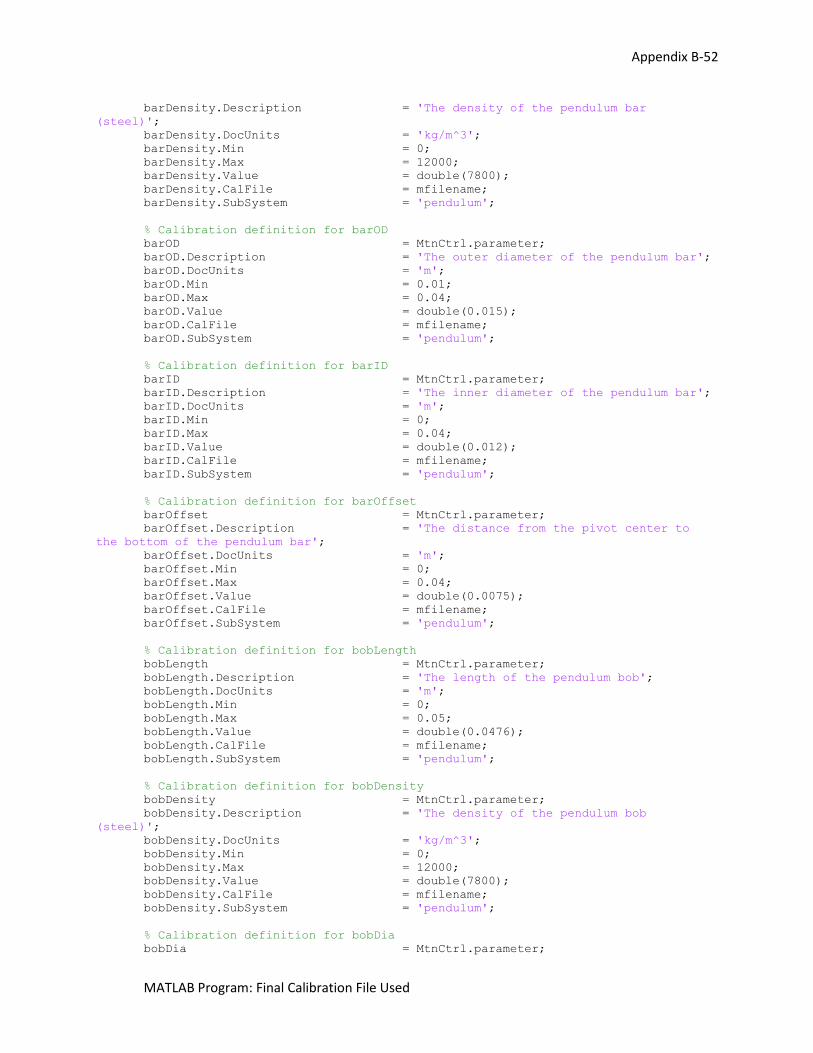
Appendix B-52
MATLAB Program: Final Calibration File Used
barDensity.Description = 'The density of the pendulum bar
(steel)';
barDensity.DocUnits = 'kg/m^3';
barDensity.Min = 0;
barDensity.Max = 12000;
barDensity.Value = double(7800);
barDensity.CalFile = mfilename;
barDensity.SubSystem = 'pendulum';
% Calibration definition for barOD
barOD = MtnCtrl.parameter;
barOD.Description = 'The outer diameter of the pendulum bar';
barOD.DocUnits = 'm';
barOD.Min = 0.01;
barOD.Max = 0.04;
barOD.Value = double(0.015);
barOD.CalFile = mfilename;
barOD.SubSystem = 'pendulum';
% Calibration definition for barID
barID = MtnCtrl.parameter;
barID.Description = 'The inner diameter of the pendulum bar';
barID.DocUnits = 'm';
barID.Min = 0;
barID.Max = 0.04;
barID.Value = double(0.012);
barID.CalFile = mfilename;
barID.SubSystem = 'pendulum';
% Calibration definition for barOffset
barOffset = MtnCtrl.parameter;
barOffset.Description = 'The distance from the pivot center to
the bottom of the pendulum bar';
barOffset.DocUnits = 'm';
barOffset.Min = 0;
barOffset.Max = 0.04;
barOffset.Value = double(0.0075);
barOffset.CalFile = mfilename;
barOffset.SubSystem = 'pendulum';
% Calibration definition for bobLength
bobLength = MtnCtrl.parameter;
bobLength.Description = 'The length of the pendulum bob';
bobLength.DocUnits = 'm';
bobLength.Min = 0;
bobLength.Max = 0.05;
bobLength.Value = double(0.0476);
bobLength.CalFile = mfilename;
bobLength.SubSystem = 'pendulum';
% Calibration definition for bobDensity
bobDensity = MtnCtrl.parameter;
bobDensity.Description = 'The density of the pendulum bob
(steel)';
bobDensity.DocUnits = 'kg/m^3';
bobDensity.Min = 0;
bobDensity.Max = 12000;
bobDensity.Value = double(7800);
bobDensity.CalFile = mfilename;
bobDensity.SubSystem = 'pendulum';
% Calibration definition for bobDia
bobDia = MtnCtrl.parameter;
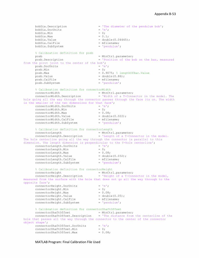
Appendix B-53
MATLAB Program: Final Calibration File Used
bobDia.Description = 'The diameter of the pendulum bob';
bobDia.DocUnits = 'm';
bobDia.Min = 0;
bobDia.Max = 0.1;
bobDia.Value = double(0.04445);
bobDia.CalFile = mfilename;
bobDia.SubSystem = 'pendulum';
% Calibration definition for posb
posb = MtnCtrl.parameter;
posb.Description = 'Position of the bob on the bar, measured
from the pivot joint to the center of the bob';
posb.DocUnits = 'm';
posb.Min = 0;
posb.Max = 0.9075; % lengthOfBar.Value
posb.Value = double(0.86);
posb.CalFile = mfilename;
posb.SubSystem = 'pendulum';
% Calibration definition for connectorWidth
connectorWidth = MtnCtrl.parameter;
connectorWidth.Description = 'Width of a T-Connector in the model. The
hole going all the way through the connector passes through the face its on. The width
is the smaller of the two dimensions for that face';
connectorWidth.DocUnits = 'm';
connectorWidth.Min = 0;
connectorWidth.Max = 0.08;
connectorWidth.Value = double(0.022);
connectorWidth.CalFile = mfilename;
connectorWidth.SubSystem = 'pendulum';
% Calibration definition for connectorLength
connectorLength = MtnCtrl.parameter;
connectorLength.Description = 'Length of a T-Connector in the model.
The hole centerline going all the way through the connector is parallel to this
dimension. The length dimension is perpendicular to the T-hole centerline';
connectorLength.DocUnits = 'm';
connectorLength.Min = 0;
connectorLength.Max = 0.08;
connectorLength.Value = double(0.032);
connectorLength.CalFile = mfilename;
connectorLength.SubSystem = 'pendulum';
% Calibration definition for connectorHeight
connectorHeight = MtnCtrl.parameter;
connectorHeight.Description = 'Height of a T-Connector in the model,
measured from the surface with the hole that does not go all the way through to the
opposite face';
connectorHeight.DocUnits = 'm';
connectorHeight.Min = 0;
connectorHeight.Max = 0.08;
connectorHeight.Value = double(0.05);
connectorHeight.CalFile = mfilename;
connectorHeight.SubSystem = 'pendulum';
% Calibration definition for connectorShaftOffset
connectorShaftOffset = MtnCtrl.parameter;
connectorShaftOffset.Description = 'The distance from the centerline of the
hole that passes all the way through the connector to the center of the connector
object shape';
connectorShaftOffset.DocUnits = 'm';
connectorShaftOffset.Min = 0;
connectorShaftOffset.Max = 0.08;
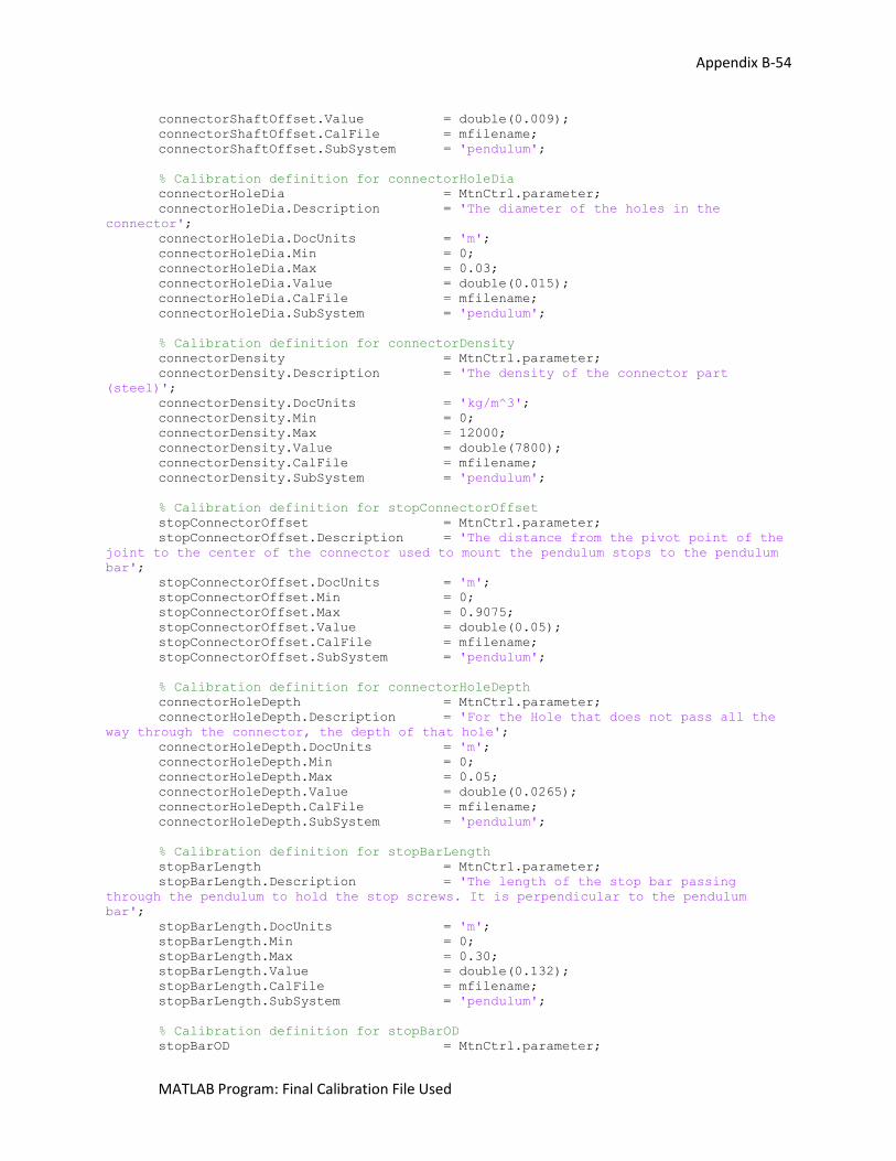
Appendix B-54
MATLAB Program: Final Calibration File Used
connectorShaftOffset.Value = double(0.009);
connectorShaftOffset.CalFile = mfilename;
connectorShaftOffset.SubSystem = 'pendulum';
% Calibration definition for connectorHoleDia
connectorHoleDia = MtnCtrl.parameter;
connectorHoleDia.Description = 'The diameter of the holes in the
connector';
connectorHoleDia.DocUnits = 'm';
connectorHoleDia.Min = 0;
connectorHoleDia.Max = 0.03;
connectorHoleDia.Value = double(0.015);
connectorHoleDia.CalFile = mfilename;
connectorHoleDia.SubSystem = 'pendulum';
% Calibration definition for connectorDensity
connectorDensity = MtnCtrl.parameter;
connectorDensity.Description = 'The density of the connector part
(steel)';
connectorDensity.DocUnits = 'kg/m^3';
connectorDensity.Min = 0;
connectorDensity.Max = 12000;
connectorDensity.Value = double(7800);
connectorDensity.CalFile = mfilename;
connectorDensity.SubSystem = 'pendulum';
% Calibration definition for stopConnectorOffset
stopConnectorOffset = MtnCtrl.parameter;
stopConnectorOffset.Description = 'The distance from the pivot point of the
joint to the center of the connector used to mount the pendulum stops to the pendulum
bar';
stopConnectorOffset.DocUnits = 'm';
stopConnectorOffset.Min = 0;
stopConnectorOffset.Max = 0.9075;
stopConnectorOffset.Value = double(0.05);
stopConnectorOffset.CalFile = mfilename;
stopConnectorOffset.SubSystem = 'pendulum';
% Calibration definition for connectorHoleDepth
connectorHoleDepth = MtnCtrl.parameter;
connectorHoleDepth.Description = 'For the Hole that does not pass all the
way through the connector, the depth of that hole';
connectorHoleDepth.DocUnits = 'm';
connectorHoleDepth.Min = 0;
connectorHoleDepth.Max = 0.05;
connectorHoleDepth.Value = double(0.0265);
connectorHoleDepth.CalFile = mfilename;
connectorHoleDepth.SubSystem = 'pendulum';
% Calibration definition for stopBarLength
stopBarLength = MtnCtrl.parameter;
stopBarLength.Description = 'The length of the stop bar passing
through the pendulum to hold the stop screws. It is perpendicular to the pendulum
bar';
stopBarLength.DocUnits = 'm';
stopBarLength.Min = 0;
stopBarLength.Max = 0.30;
stopBarLength.Value = double(0.132);
stopBarLength.CalFile = mfilename;
stopBarLength.SubSystem = 'pendulum';
% Calibration definition for stopBarOD
stopBarOD = MtnCtrl.parameter;
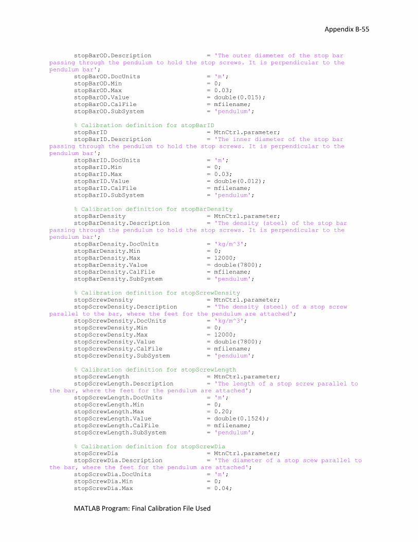
Appendix B-55
MATLAB Program: Final Calibration File Used
stopBarOD.Description = 'The outer diameter of the stop bar
passing through the pendulum to hold the stop screws. It is perpendicular to the
pendulum bar';
stopBarOD.DocUnits = 'm';
stopBarOD.Min = 0;
stopBarOD.Max = 0.03;
stopBarOD.Value = double(0.015);
stopBarOD.CalFile = mfilename;
stopBarOD.SubSystem = 'pendulum';
% Calibration definition for stopBarID
stopBarID = MtnCtrl.parameter;
stopBarID.Description = 'The inner diameter of the stop bar
passing through the pendulum to hold the stop screws. It is perpendicular to the
pendulum bar';
stopBarID.DocUnits = 'm';
stopBarID.Min = 0;
stopBarID.Max = 0.03;
stopBarID.Value = double(0.012);
stopBarID.CalFile = mfilename;
stopBarID.SubSystem = 'pendulum';
% Calibration definition for stopBarDensity
stopBarDensity = MtnCtrl.parameter;
stopBarDensity.Description = 'The density (steel) of the stop bar
passing through the pendulum to hold the stop screws. It is perpendicular to the
pendulum bar';
stopBarDensity.DocUnits = 'kg/m^3';
stopBarDensity.Min = 0;
stopBarDensity.Max = 12000;
stopBarDensity.Value = double(7800);
stopBarDensity.CalFile = mfilename;
stopBarDensity.SubSystem = 'pendulum';
% Calibration definition for stopScrewDensity
stopScrewDensity = MtnCtrl.parameter;
stopScrewDensity.Description = 'The density (steel) of a stop screw
parallel to the bar, where the feet for the pendulum are attached';
stopScrewDensity.DocUnits = 'kg/m^3';
stopScrewDensity.Min = 0;
stopScrewDensity.Max = 12000;
stopScrewDensity.Value = double(7800);
stopScrewDensity.CalFile = mfilename;
stopScrewDensity.SubSystem = 'pendulum';
% Calibration definition for stopScrewLength
stopScrewLength = MtnCtrl.parameter;
stopScrewLength.Description = 'The length of a stop screw parallel to
the bar, where the feet for the pendulum are attached';
stopScrewLength.DocUnits = 'm';
stopScrewLength.Min = 0;
stopScrewLength.Max = 0.20;
stopScrewLength.Value = double(0.1524);
stopScrewLength.CalFile = mfilename;
stopScrewLength.SubSystem = 'pendulum';
% Calibration definition for stopScrewDia
stopScrewDia = MtnCtrl.parameter;
stopScrewDia.Description = 'The diameter of a stop scew parallel to
the bar, where the feet for the pendulum are attached';
stopScrewDia.DocUnits = 'm';
stopScrewDia.Min = 0;
stopScrewDia.Max = 0.04;
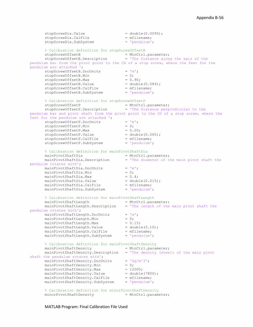
Appendix B-56
MATLAB Program: Final Calibration File Used
stopScrewDia.Value = double(0.0095);
stopScrewDia.CalFile = mfilename;
stopScrewDia.SubSystem = 'pendulum';
% Calibration definition for stopScrewOffsetB
stopScrewOffsetB = MtnCtrl.parameter;
stopScrewOffsetB.Description = 'The Distance along the axis of the
pendulum bar from the pivot point to the CG of a stop screw, where the feet for the
pendulum are attached ';
stopScrewOffsetB.DocUnits = 'm';
stopScrewOffsetB.Min = 0;
stopScrewOffsetB.Max = 0.90;
stopScrewOffsetB.Value = double(0.084);
stopScrewOffsetB.CalFile = mfilename;
stopScrewOffsetB.SubSystem = 'pendulum';
% Calibration definition for stopScrewOffsetP
stopScrewOffsetP = MtnCtrl.parameter;
stopScrewOffsetP.Description = 'The Distance perpindicular to the
pendulum bar and pivot shaft from the pivot point to the CG of a stop screw, where the
feet for the pendulum are attached ';
stopScrewOffsetP.DocUnits = 'm';
stopScrewOffsetP.Min = 0;
stopScrewOffsetP.Max = 0.20;
stopScrewOffsetP.Value = double(0.065);
stopScrewOffsetP.CalFile = mfilename;
stopScrewOffsetP.SubSystem = 'pendulum';
% Calibration definition for mainPivotShaftDia
mainPivotShaftDia = MtnCtrl.parameter;
mainPivotShaftDia.Description = 'The diameter of the main pivot shaft the
pendulum rotates with';
mainPivotShaftDia.DocUnits = 'm';
mainPivotShaftDia.Min = 0;
mainPivotShaftDia.Max = 0.4;
mainPivotShaftDia.Value = double(0.015);
mainPivotShaftDia.CalFile = mfilename;
mainPivotShaftDia.SubSystem = 'pendulum';
% Calibration definition for mainPivotShaftLength
mainPivotShaftLength = MtnCtrl.parameter;
mainPivotShaftLength.Description = 'The length of the main pivot shaft the
pendulum rotates with';
mainPivotShaftLength.DocUnits = 'm';
mainPivotShaftLength.Min = 0;
mainPivotShaftLength.Max = 0.15;
mainPivotShaftLength.Value = double(0.10);
mainPivotShaftLength.CalFile = mfilename;
mainPivotShaftLength.SubSystem = 'pendulum';
% Calibration definition for mainPivotShaftDensity
mainPivotShaftDensity = MtnCtrl.parameter;
mainPivotShaftDensity.Description = 'The density (steel) of the main pivot
shaft the pendulum rotates with';
mainPivotShaftDensity.DocUnits = 'kg/m^3';
mainPivotShaftDensity.Min = 0;
mainPivotShaftDensity.Max = 12000;
mainPivotShaftDensity.Value = double(7800);
mainPivotShaftDensity.CalFile = mfilename;
mainPivotShaftDensity.SubSystem = 'pendulum';
% Calibration definition for minorPivotShaftDensity
minorPivotShaftDensity = MtnCtrl.parameter;
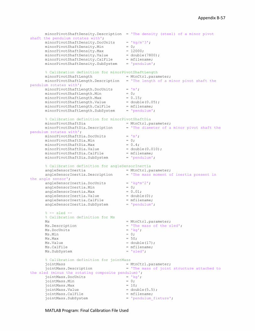
Appendix B-57
MATLAB Program: Final Calibration File Used
minorPivotShaftDensity.Description = 'The density (steel) of a minor pivot
shaft the pendulum rotates with';
minorPivotShaftDensity.DocUnits = 'kg/m^3';
minorPivotShaftDensity.Min = 0;
minorPivotShaftDensity.Max = 12000;
minorPivotShaftDensity.Value = double(7800);
minorPivotShaftDensity.CalFile = mfilename;
minorPivotShaftDensity.SubSystem = 'pendulum';
% Calibration definition for minorPivotShaftLength
minorPivotShaftLength = MtnCtrl.parameter;
minorPivotShaftLength.Description = 'The length of a minor pivot shaft the
pendulum rotates with';
minorPivotShaftLength.DocUnits = 'm';
minorPivotShaftLength.Min = 0;
minorPivotShaftLength.Max = 0.15;
minorPivotShaftLength.Value = double(0.05);
minorPivotShaftLength.CalFile = mfilename;
minorPivotShaftLength.SubSystem = 'pendulum';
% Calibration definition for minorPivotShaftDia
minorPivotShaftDia = MtnCtrl.parameter;
minorPivotShaftDia.Description = 'The diameter of a minor pivot shaft the
pendulum rotates with';
minorPivotShaftDia.DocUnits = 'm';
minorPivotShaftDia.Min = 0;
minorPivotShaftDia.Max = 0.4;
minorPivotShaftDia.Value = double(0.010);
minorPivotShaftDia.CalFile = mfilename;
minorPivotShaftDia.SubSystem = 'pendulum';
% Calibration definition for angleSensorInertia
angleSensorInertia = MtnCtrl.parameter;
angleSensorInertia.Description = 'The mass moment of inertia present in
the angle sensor';
angleSensorInertia.DocUnits = 'kg*m^2';
angleSensorInertia.Min = 0;
angleSensorInertia.Max = 0.01;
angleSensorInertia.Value = double(0);
angleSensorInertia.CalFile = mfilename;
angleSensorInertia.SubSystem = 'pendulum';
% -- sled --
% Calibration definition for Ms
Ms = MtnCtrl.parameter;
Ms.Description = 'The mass of the sled';
Ms.DocUnits = 'kg';
Ms.Min = 0;
Ms.Max = 50;
Ms.Value = double(17);
Ms.CalFile = mfilename;
Ms.SubSystem = 'sled';
% Calibration definition for jointMass
jointMass = MtnCtrl.parameter;
jointMass.Description = 'The mass of joint structure attached to
the sled (minus the rotating composite pendulum)';
jointMass.DocUnits = 'kg';
jointMass.Min = 0;
jointMass.Max = 10;
jointMass.Value = double(5.5);
jointMass.CalFile = mfilename;
jointMass.SubSystem = 'pendulum_fixture';
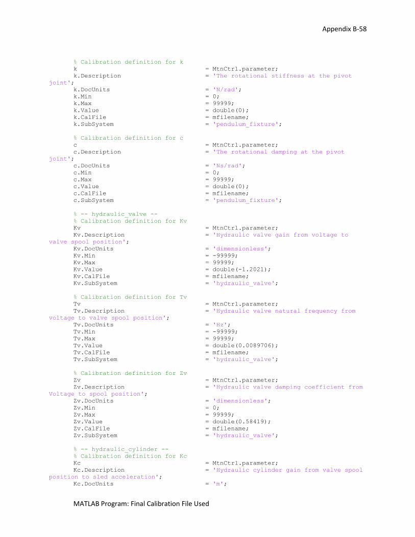
Appendix B-58
MATLAB Program: Final Calibration File Used
% Calibration definition for k
k = MtnCtrl.parameter;
k.Description = 'The rotational stiffness at the pivot
joint';
k.DocUnits = 'N/rad';
k.Min = 0;
k.Max = 99999;
k.Value = double(0);
k.CalFile = mfilename;
k.SubSystem = 'pendulum_fixture';
% Calibration definition for c
c = MtnCtrl.parameter;
c.Description = 'The rotational damping at the pivot
joint';
c.DocUnits = 'Ns/rad';
c.Min = 0;
c.Max = 99999;
c.Value = double(0);
c.CalFile = mfilename;
c.SubSystem = 'pendulum_fixture';
% -- hydraulic_valve --
% Calibration definition for Kv
Kv = MtnCtrl.parameter;
Kv.Description = 'Hydraulic valve gain from voltage to
valve spool position';
Kv.DocUnits = 'dimensionless';
Kv.Min = -99999;
Kv.Max = 99999;
Kv.Value = double(-1.2021);
Kv.CalFile = mfilename;
Kv.SubSystem = 'hydraulic_valve';
% Calibration definition for Tv
Tv = MtnCtrl.parameter;
Tv.Description = 'Hydraulic valve natural frequency from
voltage to valve spool position';
Tv.DocUnits = 'Hz';
Tv.Min = -99999;
Tv.Max = 99999;
Tv.Value = double(0.0089706);
Tv.CalFile = mfilename;
Tv.SubSystem = 'hydraulic_valve';
% Calibration definition for Zv
Zv = MtnCtrl.parameter;
Zv.Description = 'Hydraulic valve damping coefficient from
Voltage to spool position';
Zv.DocUnits = 'dimensionless';
Zv.Min = 0;
Zv.Max = 99999;
Zv.Value = double(0.58419);
Zv.CalFile = mfilename;
Zv.SubSystem = 'hydraulic_valve';
% -- hydraulic_cylinder --
% Calibration definition for Kc
Kc = MtnCtrl.parameter;
Kc.Description = 'Hydraulic cylinder gain from valve spool
position to sled acceleration';
Kc.DocUnits = 'm';
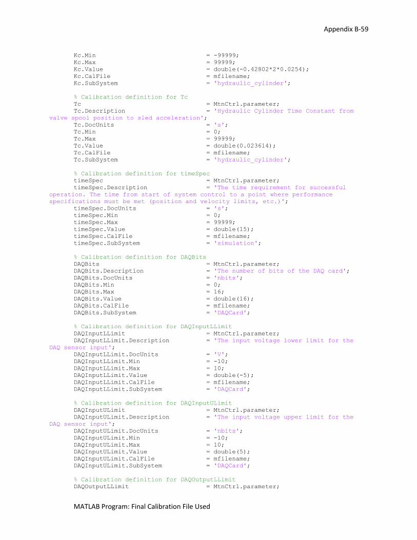
Appendix B-59
MATLAB Program: Final Calibration File Used
Kc.Min = -99999;
Kc.Max = 99999;
Kc.Value = double(-0.42802*2*0.0254);
Kc.CalFile = mfilename;
Kc.SubSystem = 'hydraulic_cylinder';
% Calibration definition for Tc
Tc = MtnCtrl.parameter;
Tc.Description = 'Hydraulic Cylinder Time Constant from
valve spool position to sled acceleration';
Tc.DocUnits = 's';
Tc.Min = 0;
Tc.Max = 99999;
Tc.Value = double(0.023614);
Tc.CalFile = mfilename;
Tc.SubSystem = 'hydraulic_cylinder';
% Calibration definition for timeSpec
timeSpec = MtnCtrl.parameter;
timeSpec.Description = 'The time requirement for successful
operation. The time from start of system control to a point where performance
specifications must be met (position and velocity limits, etc.)';
timeSpec.DocUnits = 's';
timeSpec.Min = 0;
timeSpec.Max = 99999;
timeSpec.Value = double(15);
timeSpec.CalFile = mfilename;
timeSpec.SubSystem = 'simulation';
% Calibration definition for DAQBits
DAQBits = MtnCtrl.parameter;
DAQBits.Description = 'The number of bits of the DAQ card';
DAQBits.DocUnits = 'nbits';
DAQBits.Min = 0;
DAQBits.Max = 16;
DAQBits.Value = double(16);
DAQBits.CalFile = mfilename;
DAQBits.SubSystem = 'DAQCard';
% Calibration definition for DAQInputLLimit
DAQInputLLimit = MtnCtrl.parameter;
DAQInputLLimit.Description = 'The input voltage lower limit for the
DAQ sensor input';
DAQInputLLimit.DocUnits = 'V';
DAQInputLLimit.Min = -10;
DAQInputLLimit.Max = 10;
DAQInputLLimit.Value = double(-5);
DAQInputLLimit.CalFile = mfilename;
DAQInputLLimit.SubSystem = 'DAQCard';
% Calibration definition for DAQInputULimit
DAQInputULimit = MtnCtrl.parameter;
DAQInputULimit.Description = 'The input voltage upper limit for the
DAQ sensor input';
DAQInputULimit.DocUnits = 'nbits';
DAQInputULimit.Min = -10;
DAQInputULimit.Max = 10;
DAQInputULimit.Value = double(5);
DAQInputULimit.CalFile = mfilename;
DAQInputULimit.SubSystem = 'DAQCard';
% Calibration definition for DAQOutputLLimit
DAQOutputLLimit = MtnCtrl.parameter;
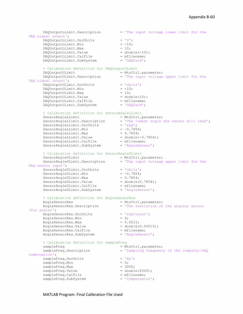
Appendix B-60
MATLAB Program: Final Calibration File Used
DAQOutputLLimit.Description = 'The input voltage lower limit for the
DAQ signal output';
DAQOutputLLimit.DocUnits = 'V';
DAQOutputLLimit.Min = -10;
DAQOutputLLimit.Max = 10;
DAQOutputLLimit.Value = double(-10);
DAQOutputLLimit.CalFile = mfilename;
DAQOutputLLimit.SubSystem = 'DAQCard';
% Calibration definition for DAQOutputULimit
DAQOutputULimit = MtnCtrl.parameter;
DAQOutputULimit.Description = 'The input voltage upper limit for the
DAQ signal output';
DAQOutputULimit.DocUnits = 'nbits';
DAQOutputULimit.Min = -10;
DAQOutputULimit.Max = 10;
DAQOutputULimit.Value = double(10);
DAQOutputULimit.CalFile = mfilename;
DAQOutputULimit.SubSystem = 'DAQCard';
% Calibration definition for SensorAngleLLimit
SensorAngleLLimit = MtnCtrl.parameter;
SensorAngleLLimit.Description = 'The lowest angle the sensor will read';
SensorAngleLLimit.DocUnits = 'rad';
SensorAngleLLimit.Min = -0.7854;
SensorAngleLLimit.Max = 0.7854;
SensorAngleLLimit.Value = double(-0.7854);
SensorAngleLLimit.CalFile = mfilename;
SensorAngleLLimit.SubSystem = 'AngleSensor';
% Calibration definition for SensorAngleULimit
SensorAngleULimit = MtnCtrl.parameter;
SensorAngleULimit.Description = 'The input voltage upper limit for the
DAQ sensor input';
SensorAngleULimit.DocUnits = 'nbits';
SensorAngleULimit.Min = -0.7854;
SensorAngleULimit.Max = 0.7854;
SensorAngleULimit.Value = double(0.7854);
SensorAngleULimit.CalFile = mfilename;
SensorAngleULimit.SubSystem = 'AngleSensor';
% Calibration definition for AngleSensorRes
AngleSensorRes = MtnCtrl.parameter;
AngleSensorRes.Description = 'The resolution of the angular sensor
(for angle)';
AngleSensorRes.DocUnits = 'rad/count';
AngleSensorRes.Min = 0;
AngleSensorRes.Max = 0.0015;
AngleSensorRes.Value = double(0.00015);
AngleSensorRes.CalFile = mfilename;
AngleSensorRes.SubSystem = 'AngleSensor';
% Calibration definition for sampleFreq
sampleFreq = MtnCtrl.parameter;
sampleFreq.Description = 'Sampling frequency of the computer/DAQ
combination';
sampleFreq.DocUnits = 'Hz';
sampleFreq.Min = 0;
sampleFreq.Max = 3000;
sampleFreq.Value = double(2000);
sampleFreq.CalFile = mfilename;
sampleFreq.SubSystem = 'Compensator';
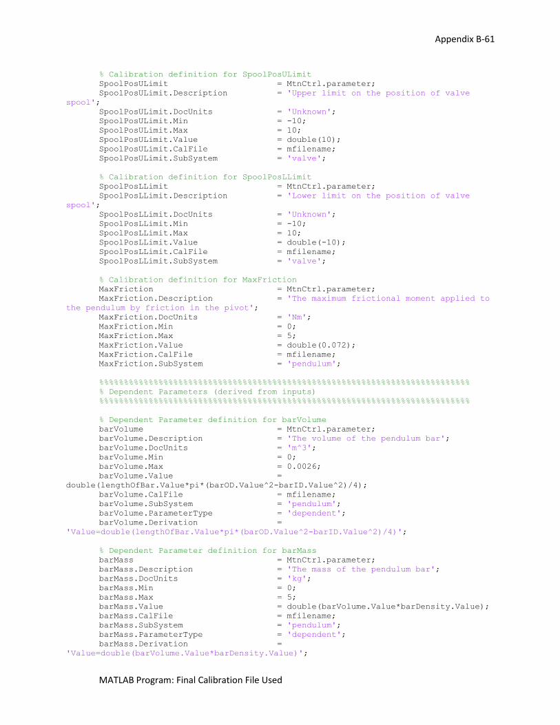
Appendix B-61
MATLAB Program: Final Calibration File Used
% Calibration definition for SpoolPosULimit
SpoolPosULimit = MtnCtrl.parameter;
SpoolPosULimit.Description = 'Upper limit on the position of valve
spool';
SpoolPosULimit.DocUnits = 'Unknown';
SpoolPosULimit.Min = -10;
SpoolPosULimit.Max = 10;
SpoolPosULimit.Value = double(10);
SpoolPosULimit.CalFile = mfilename;
SpoolPosULimit.SubSystem = 'valve';
% Calibration definition for SpoolPosLLimit
SpoolPosLLimit = MtnCtrl.parameter;
SpoolPosLLimit.Description = 'Lower limit on the position of valve
spool';
SpoolPosLLimit.DocUnits = 'Unknown';
SpoolPosLLimit.Min = -10;
SpoolPosLLimit.Max = 10;
SpoolPosLLimit.Value = double(-10);
SpoolPosLLimit.CalFile = mfilename;
SpoolPosLLimit.SubSystem = 'valve';
% Calibration definition for MaxFriction
MaxFriction = MtnCtrl.parameter;
MaxFriction.Description = 'The maximum frictional moment applied to
the pendulum by friction in the pivot';
MaxFriction.DocUnits = 'Nm';
MaxFriction.Min = 0;
MaxFriction.Max = 5;
MaxFriction.Value = double(0.072);
MaxFriction.CalFile = mfilename;
MaxFriction.SubSystem = 'pendulum';
%%%%%%%%%%%%%%%%%%%%%%%%%%%%%%%%%%%%%%%%%%%%%%%%%%%%%%%%%%%%%%%%%%%%%%%%%%%
% Dependent Parameters (derived from inputs)
%%%%%%%%%%%%%%%%%%%%%%%%%%%%%%%%%%%%%%%%%%%%%%%%%%%%%%%%%%%%%%%%%%%%%%%%%%%
% Dependent Parameter definition for barVolume
barVolume = MtnCtrl.parameter;
barVolume.Description = 'The volume of the pendulum bar';
barVolume.DocUnits = 'm^3';
barVolume.Min = 0;
barVolume.Max = 0.0026;
barVolume.Value =
double(lengthOfBar.Value*pi*(barOD.Value^2-barID.Value^2)/4);
barVolume.CalFile = mfilename;
barVolume.SubSystem = 'pendulum';
barVolume.ParameterType = 'dependent';
barVolume.Derivation =
'Value=double(lengthOfBar.Value*pi*(barOD.Value^2-barID.Value^2)/4)';
% Dependent Parameter definition for barMass
barMass = MtnCtrl.parameter;
barMass.Description = 'The mass of the pendulum bar';
barMass.DocUnits = 'kg';
barMass.Min = 0;
barMass.Max = 5;
barMass.Value = double(barVolume.Value*barDensity.Value);
barMass.CalFile = mfilename;
barMass.SubSystem = 'pendulum';
barMass.ParameterType = 'dependent';
barMass.Derivation =
'Value=double(barVolume.Value*barDensity.Value)';
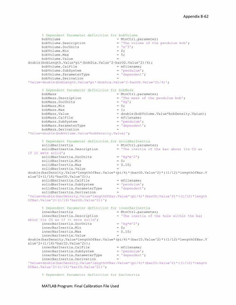
Appendix B-62
MATLAB Program: Final Calibration File Used
% Dependent Parameter definition for bobVolume
bobVolume = MtnCtrl.parameter;
bobVolume.Description = 'The volume of the pendulum bob';
bobVolume.DocUnits = 'm^3';
bobVolume.Min = 0;
bobVolume.Max = 5;
bobVolume.Value =
double(bobLength.Value*pi*(bobDia.Value^2-barOD.Value^2)/4);
bobVolume.CalFile = mfilename;
bobVolume.SubSystem = 'pendulum';
bobVolume.ParameterType = 'dependent';
bobVolume.Derivation =
'Value=double(bobLength.Value*pi*(bobDia.Value^2-barOD.Value^2)/4)';
% Dependent Parameter definition for bobMass
bobMass = MtnCtrl.parameter;
bobMass.Description = 'The mass of the pendulum bob';
bobMass.DocUnits = 'kg';
bobMass.Min = 0;
bobMass.Max = 1;
bobMass.Value = double(bobVolume.Value*bobDensity.Value);
bobMass.CalFile = mfilename;
bobMass.SubSystem = 'pendulum';
bobMass.ParameterType = 'dependent';
bobMass.Derivation =
'Value=double(bobVolume.Value*bobDensity.Value)';
% Dependent Parameter definition for solidBarInertia
solidBarInertia = MtnCtrl.parameter;
solidBarInertia.Description = 'The inertia of the bar about its CG as
if it were solid';
solidBarInertia.DocUnits = 'kg*m^2';
solidBarInertia.Min = 0;
solidBarInertia.Max = 0.10;
solidBarInertia.Value =
double(barDensity.Value*lengthOfBar.Value*(pi/4)*(barOD.Value^2)*((1/12)*lengthOfBar.V
alue^2+(1/16)*barOD.Value^2));
solidBarInertia.CalFile = mfilename;
solidBarInertia.SubSystem = 'pendulum';
solidBarInertia.ParameterType = 'dependent';
solidBarInertia.Derivation =
'Value=double(barDensity.Value*lengthOfBar.Value*(pi/4)*(barOD.Value^2)*((1/12)*length
OfBar.Value^2+(1/16)*barOD.Value^2))';
% Dependent Parameter definition for innerBarInertia
innerBarInertia = MtnCtrl.parameter;
innerBarInertia.Description = 'The inertia of the hole within the bar
about its CG as if it were solid';
innerBarInertia.DocUnits = 'kg*m^2';
innerBarInertia.Min = 0;
innerBarInertia.Max = 0.10;
innerBarInertia.Value =
double(barDensity.Value*lengthOfBar.Value*(pi/4)*(barID.Value^2)*((1/12)*lengthOfBar.V
alue^2+(1/16)*barID.Value^2));
innerBarInertia.CalFile = mfilename;
innerBarInertia.SubSystem = 'pendulum';
innerBarInertia.ParameterType = 'dependent';
innerBarInertia.Derivation =
'Value=double(barDensity.Value*lengthOfBar.Value*(pi/4)*(barID.Value^2)*((1/12)*length
OfBar.Value^2+(1/16)*barID.Value^2))';
% Dependent Parameter definition for barInertia
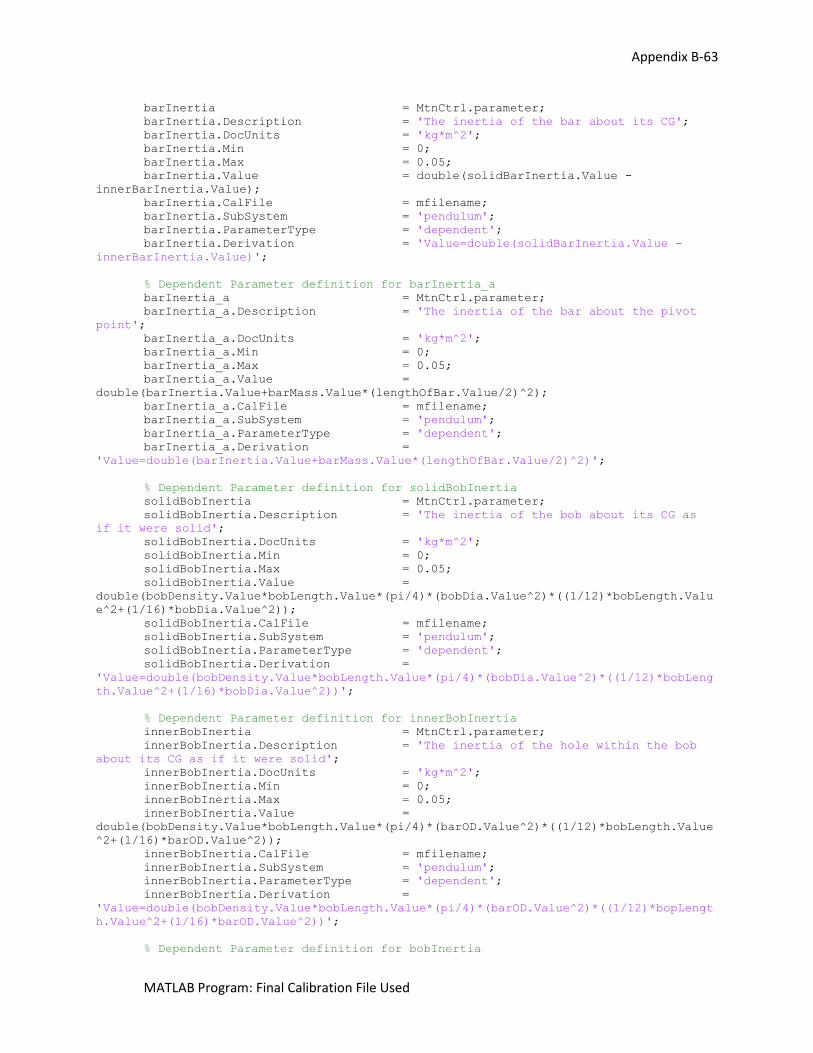
Appendix B-63
MATLAB Program: Final Calibration File Used
barInertia = MtnCtrl.parameter;
barInertia.Description = 'The inertia of the bar about its CG';
barInertia.DocUnits = 'kg*m^2';
barInertia.Min = 0;
barInertia.Max = 0.05;
barInertia.Value = double(solidBarInertia.Value -
innerBarInertia.Value);
barInertia.CalFile = mfilename;
barInertia.SubSystem = 'pendulum';
barInertia.ParameterType = 'dependent';
barInertia.Derivation = 'Value=double(solidBarInertia.Value -
innerBarInertia.Value)';
% Dependent Parameter definition for barInertia_a
barInertia_a = MtnCtrl.parameter;
barInertia_a.Description = 'The inertia of the bar about the pivot
point';
barInertia_a.DocUnits = 'kg*m^2';
barInertia_a.Min = 0;
barInertia_a.Max = 0.05;
barInertia_a.Value =
double(barInertia.Value+barMass.Value*(lengthOfBar.Value/2)^2);
barInertia_a.CalFile = mfilename;
barInertia_a.SubSystem = 'pendulum';
barInertia_a.ParameterType = 'dependent';
barInertia_a.Derivation =
'Value=double(barInertia.Value+barMass.Value*(lengthOfBar.Value/2)^2)';
% Dependent Parameter definition for solidBobInertia
solidBobInertia = MtnCtrl.parameter;
solidBobInertia.Description = 'The inertia of the bob about its CG as
if it were solid';
solidBobInertia.DocUnits = 'kg*m^2';
solidBobInertia.Min = 0;
solidBobInertia.Max = 0.05;
solidBobInertia.Value =
double(bobDensity.Value*bobLength.Value*(pi/4)*(bobDia.Value^2)*((1/12)*bobLength.Valu
e^2+(1/16)*bobDia.Value^2));
solidBobInertia.CalFile = mfilename;
solidBobInertia.SubSystem = 'pendulum';
solidBobInertia.ParameterType = 'dependent';
solidBobInertia.Derivation =
'Value=double(bobDensity.Value*bobLength.Value*(pi/4)*(bobDia.Value^2)*((1/12)*bobLeng
th.Value^2+(1/16)*bobDia.Value^2))';
% Dependent Parameter definition for innerBobInertia
innerBobInertia = MtnCtrl.parameter;
innerBobInertia.Description = 'The inertia of the hole within the bob
about its CG as if it were solid';
innerBobInertia.DocUnits = 'kg*m^2';
innerBobInertia.Min = 0;
innerBobInertia.Max = 0.05;
innerBobInertia.Value =
double(bobDensity.Value*bobLength.Value*(pi/4)*(barOD.Value^2)*((1/12)*bobLength.Value
^2+(1/16)*barOD.Value^2));
innerBobInertia.CalFile = mfilename;
innerBobInertia.SubSystem = 'pendulum';
innerBobInertia.ParameterType = 'dependent';
innerBobInertia.Derivation =
'Value=double(bobDensity.Value*bobLength.Value*(pi/4)*(barOD.Value^2)*((1/12)*bopLengt
h.Value^2+(1/16)*barOD.Value^2))';
% Dependent Parameter definition for bobInertia
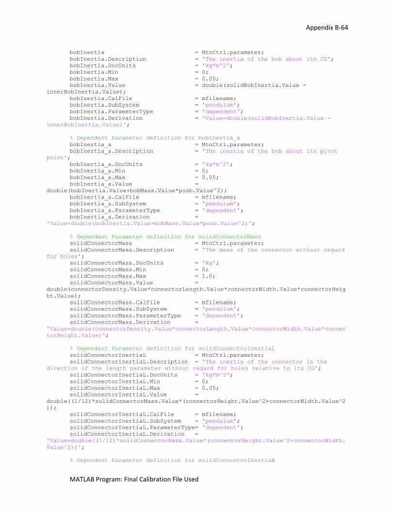
Appendix B-64
MATLAB Program: Final Calibration File Used
bobInertia = MtnCtrl.parameter;
bobInertia.Description = 'The inertia of the bob about its CG';
bobInertia.DocUnits = 'kg*m^2';
bobInertia.Min = 0;
bobInertia.Max = 0.05;
bobInertia.Value = double(solidBobInertia.Value -
innerBobInertia.Value);
bobInertia.CalFile = mfilename;
bobInertia.SubSystem = 'pendulum';
bobInertia.ParameterType = 'dependent';
bobInertia.Derivation = 'Value=double(solidBobInertia.Value -
innerBobInertia.Value)';
% Dependent Parameter definition for bobInertia_a
bobInertia_a = MtnCtrl.parameter;
bobInertia_a.Description = 'The inertia of the bob about its pivot
point';
bobInertia_a.DocUnits = 'kg*m^2';
bobInertia_a.Min = 0;
bobInertia_a.Max = 0.05;
bobInertia_a.Value =
double(bobInertia.Value+bobMass.Value*posb.Value^2);
bobInertia_a.CalFile = mfilename;
bobInertia_a.SubSystem = 'pendulum';
bobInertia_a.ParameterType = 'dependent';
bobInertia_a.Derivation =
'Value=double(bobInertia.Value+bobMass.Value*posb.Value^2)';
% Dependent Parameter definition for solidConnectorMass
solidConnectorMass = MtnCtrl.parameter;
solidConnectorMass.Description = 'The mass of the connector without regard
for holes';
solidConnectorMass.DocUnits = 'kg';
solidConnectorMass.Min = 0;
solidConnectorMass.Max = 1.0;
solidConnectorMass.Value =
double(connectorDensity.Value*connectorLength.Value*connectorWidth.Value*connectorHeig
ht.Value);
solidConnectorMass.CalFile = mfilename;
solidConnectorMass.SubSystem = 'pendulum';
solidConnectorMass.ParameterType = 'dependent';
solidConnectorMass.Derivation =
'Value=double(connectorDensity.Value*connectorLength.Value*connectorWidth.Value*connec
torHeight.Value)';
% Dependent Parameter definition for solidConnectorInertiaL
solidConnectorInertiaL = MtnCtrl.parameter;
solidConnectorInertiaL.Description = 'The inertia of the connector in the
direction of the length parameter without regard for holes relative to its CG';
solidConnectorInertiaL.DocUnits = 'kg*m^2';
solidConnectorInertiaL.Min = 0;
solidConnectorInertiaL.Max = 0.05;
solidConnectorInertiaL.Value =
double((1/12)*solidConnectorMass.Value*(connectorHeight.Value^2+connectorWidth.Value^2
));
solidConnectorInertiaL.CalFile = mfilename;
solidConnectorInertiaL.SubSystem = 'pendulum';
solidConnectorInertiaL.ParameterType= 'dependent';
solidConnectorInertiaL.Derivation =
'Value=double((1/12)*solidConnectorMass.Value*(connectorHeight.Value^2+connectorWidth.
Value^2))';
% Dependent Parameter definition for solidConnectorInertiaW
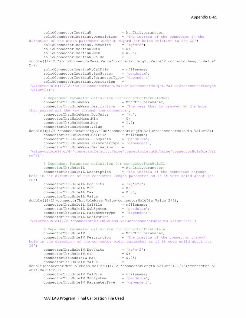
Appendix B-65
MATLAB Program: Final Calibration File Used
solidConnectorInertiaW = MtnCtrl.parameter;
solidConnectorInertiaW.Description = 'The inertia of the connector in the
direction of the width parameter without regard for holes relative to its CG';
solidConnectorInertiaW.DocUnits = 'kg*m^2';
solidConnectorInertiaW.Min = 0;
solidConnectorInertiaW.Max = 0.05;
solidConnectorInertiaW.Value =
double((1/12)*solidConnectorMass.Value*(connectorHeight.Value^2+connectorLength.Value^
2));
solidConnectorInertiaW.CalFile = mfilename;
solidConnectorInertiaW.SubSystem = 'pendulum';
solidConnectorInertiaW.ParameterType= 'dependent';
solidConnectorInertiaW.Derivation =
'Value=double((1/12)*solidConnectorMass.Value*(connectorHeight.Value^2+connectorLength
.Value^2))';
% Dependent Parameter definition for connectorThruHoleMass
connectorThruHoleMass = MtnCtrl.parameter;
connectorThruHoleMass.Description = 'The mass that is removed by the hole
that passes all the way through the connector';
connectorThruHoleMass.DocUnits = 'kg';
connectorThruHoleMass.Min = 0;
connectorThruHoleMass.Max = 1.0;
connectorThruHoleMass.Value =
double((pi/4)*connectorDensity.Value*connectorLength.Value*connectorHoleDia.Value^2);
connectorThruHoleMass.CalFile = mfilename;
connectorThruHoleMass.SubSystem = 'pendulum';
connectorThruHoleMass.ParameterType = 'dependent';
connectorThruHoleMass.Derivation =
'Value=double((pi/4)*connectorDensity.Value*connectorLength.Value*connectorHoleDia.Val
ue^2)';
% Dependent Parameter definition for connectorThruHoleIL
connectorThruHoleIL = MtnCtrl.parameter;
connectorThruHoleIL.Description = 'The inertia of the connector through
hole in the direction of the connector length parameter as if it were solid about its
CG';
connectorThruHoleIL.DocUnits = 'kg*m^2';
connectorThruHoleIL.Min = 0;
connectorThruHoleIL.Max = 0.05;
connectorThruHoleIL.Value =
double((1/2)*connectorThruHoleMass.Value*connectorHoleDia.Value^2/4);
connectorThruHoleIL.CalFile = mfilename;
connectorThruHoleIL.SubSystem = 'pendulum';
connectorThruHoleIL.ParameterType = 'dependent';
connectorThruHoleIL.Derivation =
'Value=double((1/2)*connectorThruHoleMass.Value*connectorHoleDia.Value^2/4)';
% Dependent Parameter definition for connectorThruHoleIW
connectorThruHoleIW = MtnCtrl.parameter;
connectorThruHoleIW.Description = 'The inertia of the connector through
hole in the direction of the connector width parameter as if it were solid about its
CG';
connectorThruHoleIW.DocUnits = 'kg*m^2';
connectorThruHoleIW.Min = 0;
connectorThruhHoleIW.Max = 0.05;
connectorThruHoleIW.Value =
double(connectorThruHoleMass.Value*((1/12)*connectorLength.Value^2+(1/16)*connectorHol
eDia.Value^2));
connectorThruHoleIW.CalFile = mfilename;
connectorThruHoleIW.SubSystem = 'pendulum';
connectorThruHoleIW.ParameterType = 'dependent';
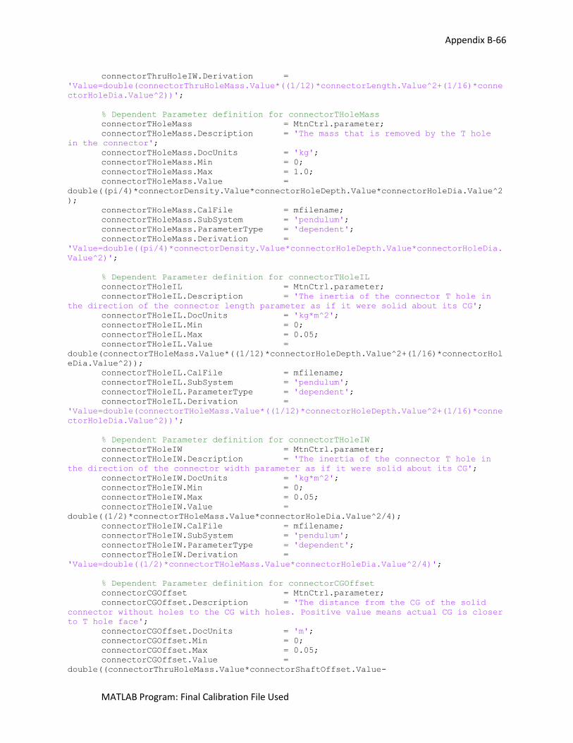
Appendix B-66
MATLAB Program: Final Calibration File Used
connectorThruHoleIW.Derivation =
'Value=double(connectorThruHoleMass.Value*((1/12)*connectorLength.Value^2+(1/16)*conne
ctorHoleDia.Value^2))';
% Dependent Parameter definition for connectorTHoleMass
connectorTHoleMass = MtnCtrl.parameter;
connectorTHoleMass.Description = 'The mass that is removed by the T hole
in the connector';
connectorTHoleMass.DocUnits = 'kg';
connectorTHoleMass.Min = 0;
connectorTHoleMass.Max = 1.0;
connectorTHoleMass.Value =
double((pi/4)*connectorDensity.Value*connectorHoleDepth.Value*connectorHoleDia.Value^2
);
connectorTHoleMass.CalFile = mfilename;
connectorTHoleMass.SubSystem = 'pendulum';
connectorTHoleMass.ParameterType = 'dependent';
connectorTHoleMass.Derivation =
'Value=double((pi/4)*connectorDensity.Value*connectorHoleDepth.Value*connectorHoleDia.
Value^2)';
% Dependent Parameter definition for connectorTHoleIL
connectorTHoleIL = MtnCtrl.parameter;
connectorTHoleIL.Description = 'The inertia of the connector T hole in
the direction of the connector length parameter as if it were solid about its CG';
connectorTHoleIL.DocUnits = 'kg*m^2';
connectorTHoleIL.Min = 0;
connectorTHoleIL.Max = 0.05;
connectorTHoleIL.Value =
double(connectorTHoleMass.Value*((1/12)*connectorHoleDepth.Value^2+(1/16)*connectorHol
eDia.Value^2));
connectorTHoleIL.CalFile = mfilename;
connectorTHoleIL.SubSystem = 'pendulum';
connectorTHoleIL.ParameterType = 'dependent';
connectorTHoleIL.Derivation =
'Value=double(connectorTHoleMass.Value*((1/12)*connectorHoleDepth.Value^2+(1/16)*conne
ctorHoleDia.Value^2))';
% Dependent Parameter definition for connectorTHoleIW
connectorTHoleIW = MtnCtrl.parameter;
connectorTHoleIW.Description = 'The inertia of the connector T hole in
the direction of the connector width parameter as if it were solid about its CG';
connectorTHoleIW.DocUnits = 'kg*m^2';
connectorTHoleIW.Min = 0;
connectorTHoleIW.Max = 0.05;
connectorTHoleIW.Value =
double((1/2)*connectorTHoleMass.Value*connectorHoleDia.Value^2/4);
connectorTHoleIW.CalFile = mfilename;
connectorTHoleIW.SubSystem = 'pendulum';
connectorTHoleIW.ParameterType = 'dependent';
connectorTHoleIW.Derivation =
'Value=double((1/2)*connectorTHoleMass.Value*connectorHoleDia.Value^2/4)';
% Dependent Parameter definition for connectorCGOffset
connectorCGOffset = MtnCtrl.parameter;
connectorCGOffset.Description = 'The distance from the CG of the solid
connector without holes to the CG with holes. Positive value means actual CG is closer
to T hole face';
connectorCGOffset.DocUnits = 'm';
connectorCGOffset.Min = 0;
connectorCGOffset.Max = 0.05;
connectorCGOffset.Value =
double((connectorThruHoleMass.Value*connectorShaftOffset.Value-
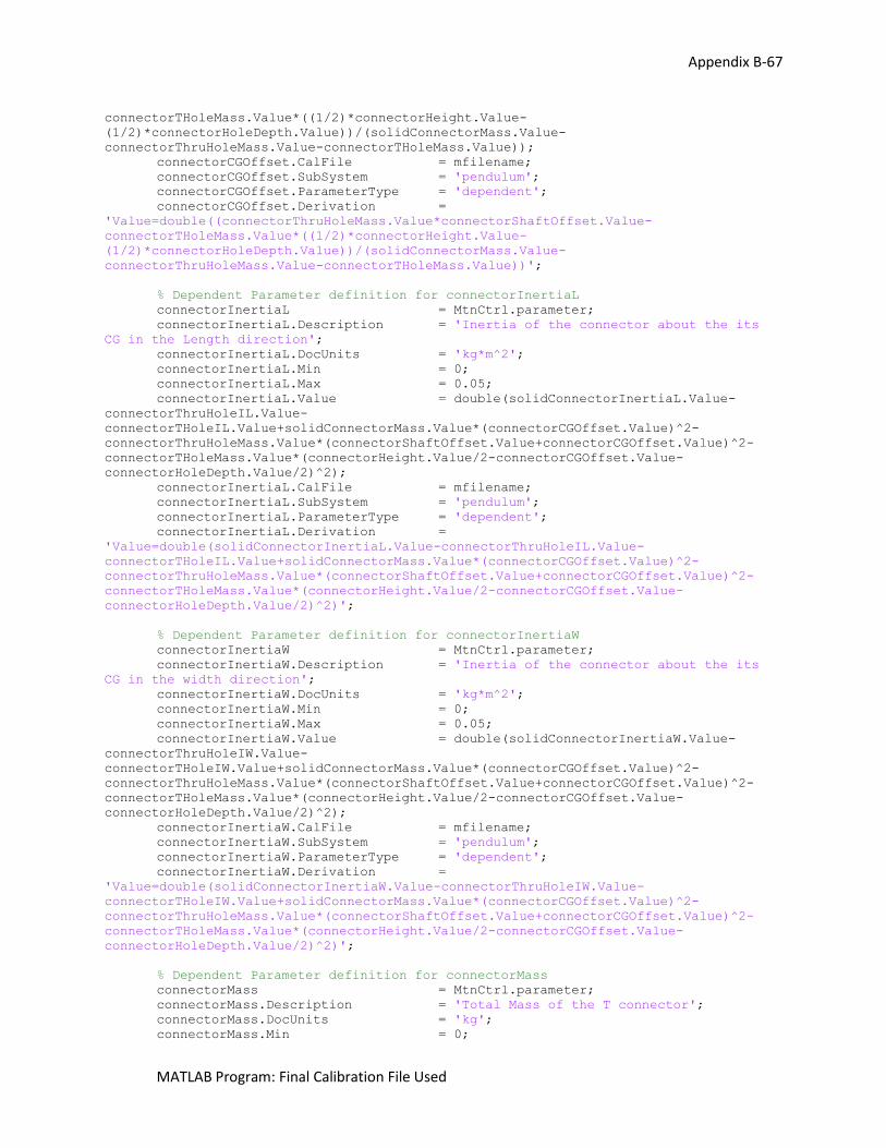
Appendix B-67
MATLAB Program: Final Calibration File Used
connectorTHoleMass.Value*((1/2)*connectorHeight.Value-
(1/2)*connectorHoleDepth.Value))/(solidConnectorMass.Value-
connectorThruHoleMass.Value-connectorTHoleMass.Value));
connectorCGOffset.CalFile = mfilename;
connectorCGOffset.SubSystem = 'pendulum';
connectorCGOffset.ParameterType = 'dependent';
connectorCGOffset.Derivation =
'Value=double((connectorThruHoleMass.Value*connectorShaftOffset.Value-
connectorTHoleMass.Value*((1/2)*connectorHeight.Value-
(1/2)*connectorHoleDepth.Value))/(solidConnectorMass.Value-
connectorThruHoleMass.Value-connectorTHoleMass.Value))';
% Dependent Parameter definition for connectorInertiaL
connectorInertiaL = MtnCtrl.parameter;
connectorInertiaL.Description = 'Inertia of the connector about the its
CG in the Length direction';
connectorInertiaL.DocUnits = 'kg*m^2';
connectorInertiaL.Min = 0;
connectorInertiaL.Max = 0.05;
connectorInertiaL.Value = double(solidConnectorInertiaL.Value-
connectorThruHoleIL.Value-
connectorTHoleIL.Value+solidConnectorMass.Value*(connectorCGOffset.Value)^2-
connectorThruHoleMass.Value*(connectorShaftOffset.Value+connectorCGOffset.Value)^2-
connectorTHoleMass.Value*(connectorHeight.Value/2-connectorCGOffset.Value-
connectorHoleDepth.Value/2)^2);
connectorInertiaL.CalFile = mfilename;
connectorInertiaL.SubSystem = 'pendulum';
connectorInertiaL.ParameterType = 'dependent';
connectorInertiaL.Derivation =
'Value=double(solidConnectorInertiaL.Value-connectorThruHoleIL.Value-
connectorTHoleIL.Value+solidConnectorMass.Value*(connectorCGOffset.Value)^2-
connectorThruHoleMass.Value*(connectorShaftOffset.Value+connectorCGOffset.Value)^2-
connectorTHoleMass.Value*(connectorHeight.Value/2-connectorCGOffset.Value-
connectorHoleDepth.Value/2)^2)';
% Dependent Parameter definition for connectorInertiaW
connectorInertiaW = MtnCtrl.parameter;
connectorInertiaW.Description = 'Inertia of the connector about the its
CG in the width direction';
connectorInertiaW.DocUnits = 'kg*m^2';
connectorInertiaW.Min = 0;
connectorInertiaW.Max = 0.05;
connectorInertiaW.Value = double(solidConnectorInertiaW.Value-
connectorThruHoleIW.Value-
connectorTHoleIW.Value+solidConnectorMass.Value*(connectorCGOffset.Value)^2-
connectorThruHoleMass.Value*(connectorShaftOffset.Value+connectorCGOffset.Value)^2-
connectorTHoleMass.Value*(connectorHeight.Value/2-connectorCGOffset.Value-
connectorHoleDepth.Value/2)^2);
connectorInertiaW.CalFile = mfilename;
connectorInertiaW.SubSystem = 'pendulum';
connectorInertiaW.ParameterType = 'dependent';
connectorInertiaW.Derivation =
'Value=double(solidConnectorInertiaW.Value-connectorThruHoleIW.Value-
connectorTHoleIW.Value+solidConnectorMass.Value*(connectorCGOffset.Value)^2-
connectorThruHoleMass.Value*(connectorShaftOffset.Value+connectorCGOffset.Value)^2-
connectorTHoleMass.Value*(connectorHeight.Value/2-connectorCGOffset.Value-
connectorHoleDepth.Value/2)^2)';
% Dependent Parameter definition for connectorMass
connectorMass = MtnCtrl.parameter;
connectorMass.Description = 'Total Mass of the T connector';
connectorMass.DocUnits = 'kg';
connectorMass.Min = 0;
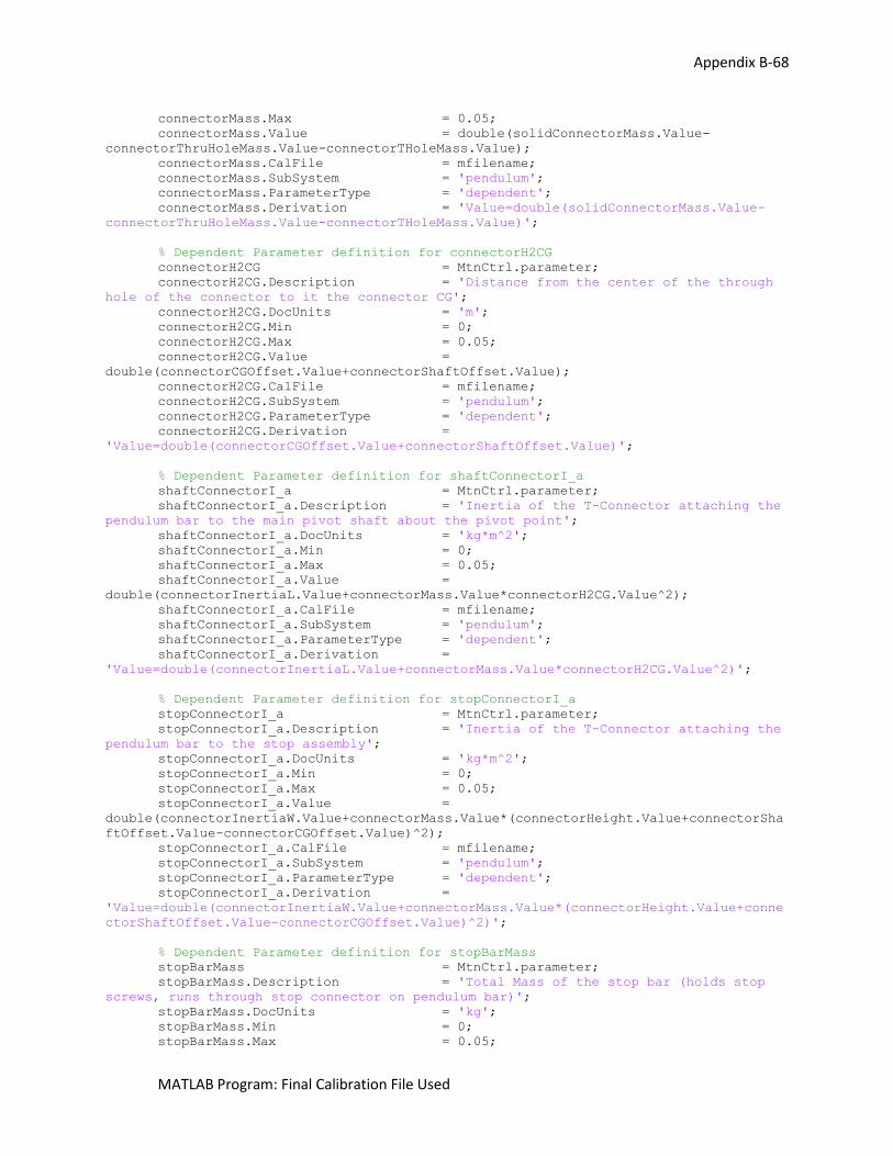
Appendix B-68
MATLAB Program: Final Calibration File Used
connectorMass.Max = 0.05;
connectorMass.Value = double(solidConnectorMass.Value-
connectorThruHoleMass.Value-connectorTHoleMass.Value);
connectorMass.CalFile = mfilename;
connectorMass.SubSystem = 'pendulum';
connectorMass.ParameterType = 'dependent';
connectorMass.Derivation = 'Value=double(solidConnectorMass.Value-
connectorThruHoleMass.Value-connectorTHoleMass.Value)';
% Dependent Parameter definition for connectorH2CG
connectorH2CG = MtnCtrl.parameter;
connectorH2CG.Description = 'Distance from the center of the through
hole of the connector to it the connector CG';
connectorH2CG.DocUnits = 'm';
connectorH2CG.Min = 0;
connectorH2CG.Max = 0.05;
connectorH2CG.Value =
double(connectorCGOffset.Value+connectorShaftOffset.Value);
connectorH2CG.CalFile = mfilename;
connectorH2CG.SubSystem = 'pendulum';
connectorH2CG.ParameterType = 'dependent';
connectorH2CG.Derivation =
'Value=double(connectorCGOffset.Value+connectorShaftOffset.Value)';
% Dependent Parameter definition for shaftConnectorI_a
shaftConnectorI_a = MtnCtrl.parameter;
shaftConnectorI_a.Description = 'Inertia of the T-Connector attaching the
pendulum bar to the main pivot shaft about the pivot point';
shaftConnectorI_a.DocUnits = 'kg*m^2';
shaftConnectorI_a.Min = 0;
shaftConnectorI_a.Max = 0.05;
shaftConnectorI_a.Value =
double(connectorInertiaL.Value+connectorMass.Value*connectorH2CG.Value^2);
shaftConnectorI_a.CalFile = mfilename;
shaftConnectorI_a.SubSystem = 'pendulum';
shaftConnectorI_a.ParameterType = 'dependent';
shaftConnectorI_a.Derivation =
'Value=double(connectorInertiaL.Value+connectorMass.Value*connectorH2CG.Value^2)';
% Dependent Parameter definition for stopConnectorI_a
stopConnectorI_a = MtnCtrl.parameter;
stopConnectorI_a.Description = 'Inertia of the T-Connector attaching the
pendulum bar to the stop assembly';
stopConnectorI_a.DocUnits = 'kg*m^2';
stopConnectorI_a.Min = 0;
stopConnectorI_a.Max = 0.05;
stopConnectorI_a.Value =
double(connectorInertiaW.Value+connectorMass.Value*(connectorHeight.Value+connectorSha
ftOffset.Value-connectorCGOffset.Value)^2);
stopConnectorI_a.CalFile = mfilename;
stopConnectorI_a.SubSystem = 'pendulum';
stopConnectorI_a.ParameterType = 'dependent';
stopConnectorI_a.Derivation =
'Value=double(connectorInertiaW.Value+connectorMass.Value*(connectorHeight.Value+conne
ctorShaftOffset.Value-connectorCGOffset.Value)^2)';
% Dependent Parameter definition for stopBarMass
stopBarMass = MtnCtrl.parameter;
stopBarMass.Description = 'Total Mass of the stop bar (holds stop
screws, runs through stop connector on pendulum bar)';
stopBarMass.DocUnits = 'kg';
stopBarMass.Min = 0;
stopBarMass.Max = 0.05;
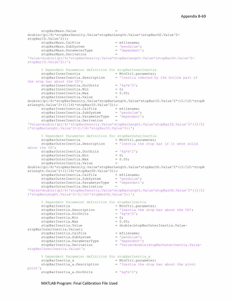
Appendix B-69
MATLAB Program: Final Calibration File Used
stopBarMass.Value =
double((pi/4)*stopBarDensity.Value*stopBarLength.Value*(stopBarOD.Value^2-
stopBarID.Value^2));
stopBarMass.CalFile = mfilename;
stopBarMass.SubSystem = 'pendulum';
stopBarMass.ParameterType = 'dependent';
stopBarMass.Derivation =
'Value=double((pi/4)*stopBarDensity.Value*stopBarLength.Value*(stopBarOD.Value^2-
stopBarID.Value^2))';
% Dependent Parameter definition for stopBarInnerInertia
stopBarInnerInertia = MtnCtrl.parameter;
stopBarInnerInertia.Description = 'Inertia removed by the hollow part of
the stop bar about the CG';
stopBarInnerInertia.DocUnits = 'kg*m^2';
stopBarInnerInertia.Min = 0;
stopBarInnerInertia.Max = 0.05;
stopBarInnerInertia.Value =
double((pi/4)*stopBarDensity.Value*stopBarLength.Value*stopBarID.Value^2*((1/12)*stopB
arLength.Value^2+(1/16)*stopBarID.Value^2));
stopBarInnerInertia.CalFile = mfilename;
stopBarInnerInertia.SubSystem = 'pendulum';
stopBarInnerInertia.ParameterType = 'dependent';
stopBarInnerInertia.Derivation =
'Value=double((pi/4)*stopBarDensity.Value*stopBarLength.Value*stopBarID.Value^2*((1/12
)*stopBarLenght.Value^2+(1/16)*stopBarID.Value^2))';
% Dependent Parameter definition for stopBarOuterInertia
stopBarOuterInertia = MtnCtrl.parameter;
stopBarOuterInertia.Description = 'Inertia the stop bar if it were solid
about the CG';
stopBarOuterInertia.DocUnits = 'kg*m^2';
stopBarOuterInertia.Min = 0;
stopBarOuterInertia.Max = 0.05;
stopBarOuterInertia.Value =
double((pi/4)*stopBarDensity.Value*stopBarLength.Value*stopBarOD.Value^2*((1/12)*stopB
arLength.Value^2+(1/16)*stopBarOD.Value^2));
stopBarOuterInertia.CalFile = mfilename;
stopBarOuterInertia.SubSystem = 'pendulum';
stopBarOuterInertia.ParameterType = 'dependent';
stopBarOuterInertia.Derivation =
'Value=double((pi/4)*stopBarDensity.Value*stopBarLength.Value*stopBarOD.Value^2*((1/12
)*stopBarLenght.Value^2+(1/16)*stopBarOD.Value^2))';
% Dependent Parameter definition for stopBarInertia
stopBarInertia = MtnCtrl.parameter;
stopBarInertia.Description = 'Inertia the stop bar about the CG';
stopBarInertia.DocUnits = 'kg*m^2';
stopBarInertia.Min = 0;
stopBarInertia.Max = 0.05;
stopBarInertia.Value = double(stopBarOuterInertia.Value-
stopBarInnerInertia.Value);
stopBarInertia.CalFile = mfilename;
stopBarInertia.SubSystem = 'pendulum';
stopBarInertia.ParameterType = 'dependent';
stopBarInertia.Derivation = 'Value=double(stopBarOuterInertia.Value-
stopBarInnerInertia.Value)';
% Dependent Parameter definition for stopBarInertia_a
stopBarInertia_a = MtnCtrl.parameter;
stopBarInertia_a.Description = 'Inertia the stop bar about the pivot
point';
stopBarInertia_a.DocUnits = 'kg*m^2';
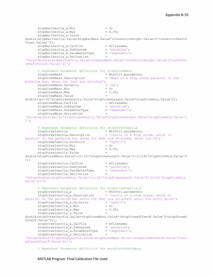
Appendix B-70
MATLAB Program: Final Calibration File Used
stopBarInertia_a.Min = 0;
stopBarInertia_a.Max = 0.05;
stopBarInertia_a.Value =
double(stopBarInertia.Value+stopBarMass.Value*(connectorHeight.Value+2*connectorShaftO
ffset.Value)^2);
stopBarInertia_a.CalFile = mfilename;
stopBarInertia_a.SubSystem = 'pendulum';
stopBarInertia_a.ParameterType = 'dependent';
stopBarInertia_a.Derivation =
'Value=double(stopBarInertia.Value+stopBarMass.Value*(connectorHeight.Value+2*connecto
rShaftOffset.Value)^2)';
% Dependent Parameter definition for stopScrewMass
stopScrewMass = MtnCtrl.parameter;
stopScrewMass.Description = 'Mass of a stop screw parallel to the
pendulum bar, where the feet are attached';
stopScrewMass.DocUnits = 'kg';
stopScrewMass.Min = 0;
stopScrewMass.Max = 0.05;
stopScrewMass.Value =
double((pi/4)*stopScrewDensity.Value*stopScrewLength.Value*stopScrewDia.Value^2);
stopScrewMass.CalFile = mfilename;
stopScrewMass.SubSystem = 'pendulum';
stopScrewMass.ParameterType = 'dependent';
stopScrewMass.Derivation =
'Value=double((pi/4)*stopScrewDensity.Value*stopScrewLength.Value*stopScrewDia.Value^2
)';
% Dependent Parameter definition for stopScrewInertia
stopScrewInertia = MtnCtrl.parameter;
stopScrewInertia.Description = 'Ineria of a stop screw, which is
parallel to the pendulum bar where the feet are attached, about its CG';
stopScrewInertia.DocUnits = 'kg*m^2';
stopScrewInertia.Min = 0;
stopScrewInertia.Max = 0.05;
stopScrewInertia.Value =
double(stopScrewMass.Value*((1/12)*stopScrewLength.Value^2+(1/16)*stopScrewDia.Value^2
));
stopScrewInertia.CalFile = mfilename;
stopScrewInertia.SubSystem = 'pendulum';
stopScrewInertia.ParameterType = 'dependent';
stopScrewInertia.Derivation =
'Value=double(stopScrewMass.Value*((1/12)*stopScrewLength.Value^2+(1/16)*stopScrewDia.
Value^2))';
% Dependent Parameter definition for stopScrewInertia_a
stopScrewInertia_a = MtnCtrl.parameter;
stopScrewInertia_a.Description = 'Ineria of a stop screw, which is
parallel to the pendulum bar where the feet are attached, about the pivot point';
stopScrewInertia_a.DocUnits = 'kg*m^2';
stopScrewInertia_a.Min = 0;
stopScrewInertia_a.Max = 0.05;
stopScrewInertia_a.Value =
double(stopScrewInertia.Value+stopScrewMass.Value*(stopScrewOffsetB.Value^2+stopScrewO
ffsetP.Value^2));
stopScrewInertia_a.CalFile = mfilename;
stopScrewInertia_a.SubSystem = 'pendulum';
stopScrewInertia_a.ParameterType = 'dependent';
stopScrewInertia_a.Derivation =
'Value=double(stopScrewInertia.Value+stopScrewMass.Value*(stopScrewOffsetB.Value^2+sto
pScrewOffsetP.Value^2))';
% Dependent Parameter definition for mainPivotShaftMass
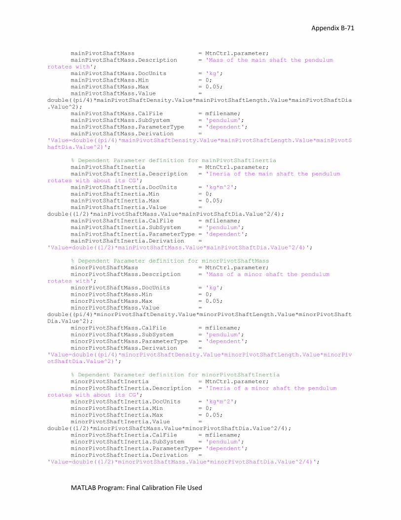
Appendix B-71
MATLAB Program: Final Calibration File Used
mainPivotShaftMass = MtnCtrl.parameter;
mainPivotShaftMass.Description = 'Mass of the main shaft the pendulum
rotates with';
mainPivotShaftMass.DocUnits = 'kg';
mainPivotShaftMass.Min = 0;
mainPivotShaftMass.Max = 0.05;
mainPivotShaftMass.Value =
double((pi/4)*mainPivotShaftDensity.Value*mainPivotShaftLength.Value*mainPivotShaftDia
.Value^2);
mainPivotShaftMass.CalFile = mfilename;
mainPivotShaftMass.SubSystem = 'pendulum';
mainPivotShaftMass.ParameterType = 'dependent';
mainPivotShaftMass.Derivation =
'Value=double((pi/4)*mainPivotShaftDensity.Value*mainPivotShaftLength.Value*mainPivotS
haftDia.Value^2)';
% Dependent Parameter definition for mainPivotShaftInertia
mainPivotShaftInertia = MtnCtrl.parameter;
mainPivotShaftInertia.Description = 'Ineria of the main shaft the pendulum
rotates with about its CG';
mainPivotShaftInertia.DocUnits = 'kg*m^2';
mainPivotShaftInertia.Min = 0;
mainPivotShaftInertia.Max = 0.05;
mainPivotShaftInertia.Value =
double((1/2)*mainPivotShaftMass.Value*mainPivotShaftDia.Value^2/4);
mainPivotShaftInertia.CalFile = mfilename;
mainPivotShaftInertia.SubSystem = 'pendulum';
mainPivotShaftInertia.ParameterType = 'dependent';
mainPivotShaftInertia.Derivation =
'Value=double((1/2)*mainPivotShaftMass.Value*mainPivotShaftDia.Value^2/4)';
% Dependent Parameter definition for minorPivotShaftMass
minorPivotShaftMass = MtnCtrl.parameter;
minorPivotShaftMass.Description = 'Mass of a minor shaft the pendulum
rotates with';
minorPivotShaftMass.DocUnits = 'kg';
minorPivotShaftMass.Min = 0;
minorPivotShaftMass.Max = 0.05;
minorPivotShaftMass.Value =
double((pi/4)*minorPivotShaftDensity.Value*minorPivotShaftLength.Value*minorPivotShaft
Dia.Value^2);
minorPivotShaftMass.CalFile = mfilename;
minorPivotShaftMass.SubSystem = 'pendulum';
minorPivotShaftMass.ParameterType = 'dependent';
minorPivotShaftMass.Derivation =
'Value=double((pi/4)*minorPivotShaftDensity.Value*minorPivotShaftLength.Value*minorPiv
otShaftDia.Value^2)';
% Dependent Parameter definition for minorPivotShaftInertia
minorPivotShaftInertia = MtnCtrl.parameter;
minorPivotShaftInertia.Description = 'Ineria of a minor shaft the pendulum
rotates with about its CG';
minorPivotShaftInertia.DocUnits = 'kg*m^2';
minorPivotShaftInertia.Min = 0;
minorPivotShaftInertia.Max = 0.05;
minorPivotShaftInertia.Value =
double((1/2)*minorPivotShaftMass.Value*minorPivotShaftDia.Value^2/4);
minorPivotShaftInertia.CalFile = mfilename;
minorPivotShaftInertia.SubSystem = 'pendulum';
minorPivotShaftInertia.ParameterType= 'dependent';
minorPivotShaftInertia.Derivation =
'Value=double((1/2)*minorPivotShaftMass.Value*minorPivotShaftDia.Value^2/4)';
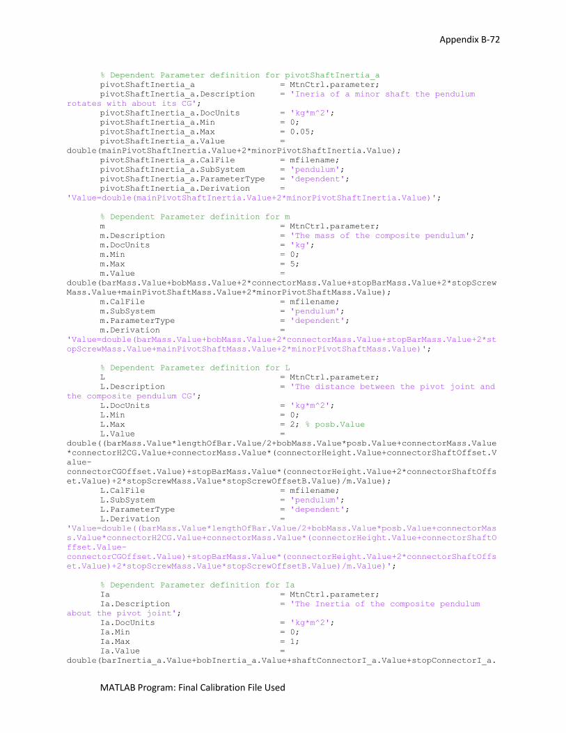
Appendix B-72
MATLAB Program: Final Calibration File Used
% Dependent Parameter definition for pivotShaftInertia_a
pivotShaftInertia_a = MtnCtrl.parameter;
pivotShaftInertia_a.Description = 'Ineria of a minor shaft the pendulum
rotates with about its CG';
pivotShaftInertia_a.DocUnits = 'kg*m^2';
pivotShaftInertia_a.Min = 0;
pivotShaftInertia_a.Max = 0.05;
pivotShaftInertia_a.Value =
double(mainPivotShaftInertia.Value+2*minorPivotShaftInertia.Value);
pivotShaftInertia_a.CalFile = mfilename;
pivotShaftInertia_a.SubSystem = 'pendulum';
pivotShaftInertia_a.ParameterType = 'dependent';
pivotShaftInertia_a.Derivation =
'Value=double(mainPivotShaftInertia.Value+2*minorPivotShaftInertia.Value)';
% Dependent Parameter definition for m
m = MtnCtrl.parameter;
m.Description = 'The mass of the composite pendulum';
m.DocUnits = 'kg';
m.Min = 0;
m.Max = 5;
m.Value =
double(barMass.Value+bobMass.Value+2*connectorMass.Value+stopBarMass.Value+2*stopScrew
Mass.Value+mainPivotShaftMass.Value+2*minorPivotShaftMass.Value);
m.CalFile = mfilename;
m.SubSystem = 'pendulum';
m.ParameterType = 'dependent';
m.Derivation =
'Value=double(barMass.Value+bobMass.Value+2*connectorMass.Value+stopBarMass.Value+2*st
opScrewMass.Value+mainPivotShaftMass.Value+2*minorPivotShaftMass.Value)';
% Dependent Parameter definition for L
L = MtnCtrl.parameter;
L.Description = 'The distance between the pivot joint and
the composite pendulum CG';
L.DocUnits = 'kg*m^2';
L.Min = 0;
L.Max = 2; % posb.Value
L.Value =
double((barMass.Value*lengthOfBar.Value/2+bobMass.Value*posb.Value+connectorMass.Value
*connectorH2CG.Value+connectorMass.Value*(connectorHeight.Value+connectorShaftOffset.V
alue-
connectorCGOffset.Value)+stopBarMass.Value*(connectorHeight.Value+2*connectorShaftOffs
et.Value)+2*stopScrewMass.Value*stopScrewOffsetB.Value)/m.Value);
L.CalFile = mfilename;
L.SubSystem = 'pendulum';
L.ParameterType = 'dependent';
L.Derivation =
'Value=double((barMass.Value*lengthOfBar.Value/2+bobMass.Value*posb.Value+connectorMas
s.Value*connectorH2CG.Value+connectorMass.Value*(connectorHeight.Value+connectorShaftO
ffset.Value-
connectorCGOffset.Value)+stopBarMass.Value*(connectorHeight.Value+2*connectorShaftOffs
et.Value)+2*stopScrewMass.Value*stopScrewOffsetB.Value)/m.Value)';
% Dependent Parameter definition for Ia
Ia = MtnCtrl.parameter;
Ia.Description = 'The Inertia of the composite pendulum
about the pivot joint';
Ia.DocUnits = 'kg*m^2';
Ia.Min = 0;
Ia.Max = 1;
Ia.Value =
double(barInertia_a.Value+bobInertia_a.Value+shaftConnectorI_a.Value+stopConnectorI_a.
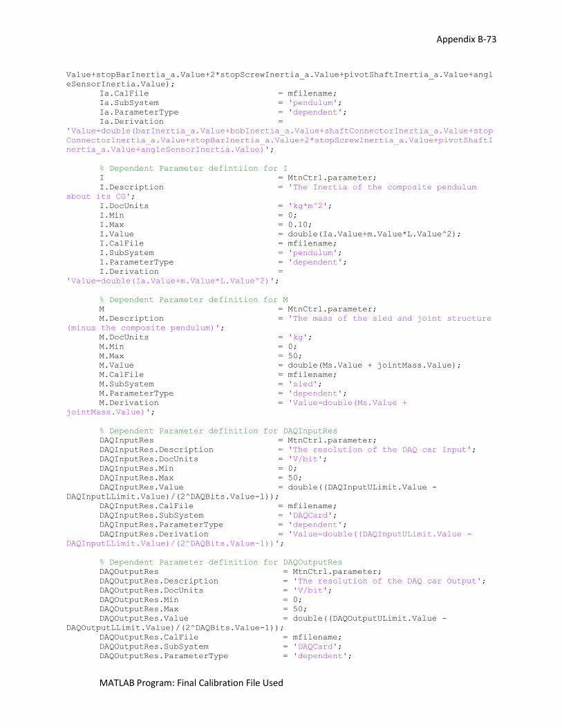
Appendix B-73
MATLAB Program: Final Calibration File Used
Value+stopBarInertia_a.Value+2*stopScrewInertia_a.Value+pivotShaftInertia_a.Value+angl
eSensorInertia.Value);
Ia.CalFile = mfilename;
Ia.SubSystem = 'pendulum';
Ia.ParameterType = 'dependent';
Ia.Derivation =
'Value=double(barInertia_a.Value+bobInertia_a.Value+shaftConnectorInertia_a.Value+stop
ConnectorInertia_a.Value+stopBarInertia_a.Value+2*stopScrewInertia_a.Value+pivotShaftI
nertia_a.Value+angleSensorInertia.Value)';
% Dependent Parameter defintiion for I
I = MtnCtrl.parameter;
I.Description = 'The Inertia of the composite pendulum
about its CG';
I.DocUnits = 'kg*m^2';
I.Min = 0;
I.Max = 0.10;
I.Value = double(Ia.Value+m.Value*L.Value^2);
I.CalFile = mfilename;
I.SubSystem = 'pendulum';
I.ParameterType = 'dependent';
I.Derivation =
'Value=double(Ia.Value+m.Value*L.Value^2)';
% Dependent Parameter definition for M
M = MtnCtrl.parameter;
M.Description = 'The mass of the sled and joint structure
(minus the composite pendulum)';
M.DocUnits = 'kg';
M.Min = 0;
M.Max = 50;
M.Value = double(Ms.Value + jointMass.Value);
M.CalFile = mfilename;
M.SubSystem = 'sled';
M.ParameterType = 'dependent';
M.Derivation = 'Value=double(Ms.Value +
jointMass.Value)';
% Dependent Parameter definition for DAQInputRes
DAQInputRes = MtnCtrl.parameter;
DAQInputRes.Description = 'The resolution of the DAQ car Input';
DAQInputRes.DocUnits = 'V/bit';
DAQInputRes.Min = 0;
DAQInputRes.Max = 50;
DAQInputRes.Value = double((DAQInputULimit.Value -
DAQInputLLimit.Value)/(2^DAQBits.Value-1));
DAQInputRes.CalFile = mfilename;
DAQInputRes.SubSystem = 'DAQCard';
DAQInputRes.ParameterType = 'dependent';
DAQInputRes.Derivation = 'Value=double((DAQInputULimit.Value -
DAQInputLLimit.Value)/(2^DAQBits.Value-1))';
% Dependent Parameter definition for DAQOutputRes
DAQOutputRes = MtnCtrl.parameter;
DAQOutputRes.Description = 'The resolution of the DAQ car Output';
DAQOutputRes.DocUnits = 'V/bit';
DAQOutputRes.Min = 0;
DAQOutputRes.Max = 50;
DAQOutputRes.Value = double((DAQOutputULimit.Value -
DAQOutputLLimit.Value)/(2^DAQBits.Value-1));
DAQOutputRes.CalFile = mfilename;
DAQOutputRes.SubSystem = 'DAQCard';
DAQOutputRes.ParameterType = 'dependent';
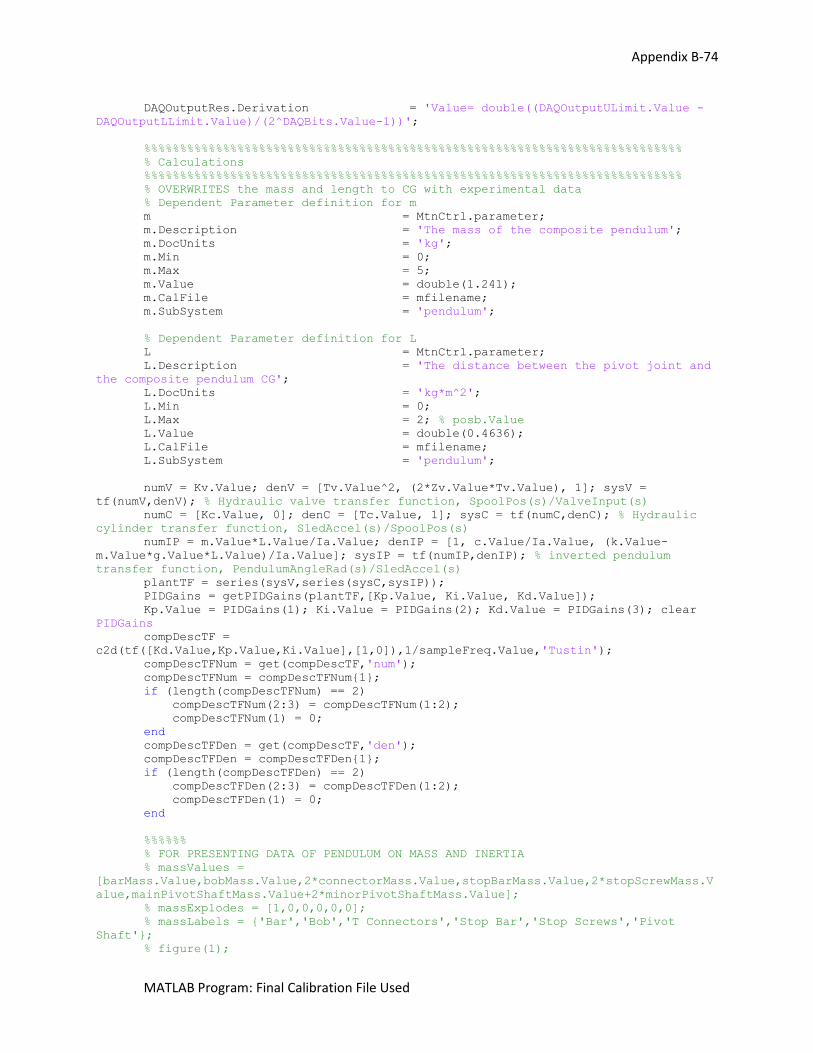
Appendix B-74
MATLAB Program: Final Calibration File Used
DAQOutputRes.Derivation = 'Value= double((DAQOutputULimit.Value -
DAQOutputLLimit.Value)/(2^DAQBits.Value-1))';
%%%%%%%%%%%%%%%%%%%%%%%%%%%%%%%%%%%%%%%%%%%%%%%%%%%%%%%%%%%%%%%%%%%%%%%%%%%
% Calculations
%%%%%%%%%%%%%%%%%%%%%%%%%%%%%%%%%%%%%%%%%%%%%%%%%%%%%%%%%%%%%%%%%%%%%%%%%%%
% OVERWRITES the mass and length to CG with experimental data
% Dependent Parameter definition for m
m = MtnCtrl.parameter;
m.Description = 'The mass of the composite pendulum';
m.DocUnits = 'kg';
m.Min = 0;
m.Max = 5;
m.Value = double(1.241);
m.CalFile = mfilename;
m.SubSystem = 'pendulum';
% Dependent Parameter definition for L
L = MtnCtrl.parameter;
L.Description = 'The distance between the pivot joint and
the composite pendulum CG';
L.DocUnits = 'kg*m^2';
L.Min = 0;
L.Max = 2; % posb.Value
L.Value = double(0.4636);
L.CalFile = mfilename;
L.SubSystem = 'pendulum';
numV = Kv.Value; denV = [Tv.Value^2, (2*Zv.Value*Tv.Value), 1]; sysV =
tf(numV,denV); % Hydraulic valve transfer function, SpoolPos(s)/ValveInput(s)
numC = [Kc.Value, 0]; denC = [Tc.Value, 1]; sysC = tf(numC,denC); % Hydraulic
cylinder transfer function, SledAccel(s)/SpoolPos(s)
numIP = m.Value*L.Value/Ia.Value; denIP = [1, c.Value/Ia.Value, (k.Value-
m.Value*g.Value*L.Value)/Ia.Value]; sysIP = tf(numIP,denIP); % inverted pendulum
transfer function, PendulumAngleRad(s)/SledAccel(s)
plantTF = series(sysV,series(sysC,sysIP));
PIDGains = getPIDGains(plantTF,[Kp.Value, Ki.Value, Kd.Value]);
Kp.Value = PIDGains(1); Ki.Value = PIDGains(2); Kd.Value = PIDGains(3); clear
PIDGains
compDescTF =
c2d(tf([Kd.Value,Kp.Value,Ki.Value],[1,0]),1/sampleFreq.Value,'Tustin');
compDescTFNum = get(compDescTF,'num');
compDescTFNum = compDescTFNum{1};
if (length(compDescTFNum) == 2)
compDescTFNum(2:3) = compDescTFNum(1:2);
compDescTFNum(1) = 0;
end
compDescTFDen = get(compDescTF,'den');
compDescTFDen = compDescTFDen{1};
if (length(compDescTFDen) == 2)
compDescTFDen(2:3) = compDescTFDen(1:2);
compDescTFDen(1) = 0;
end
%%%%%%
% FOR PRESENTING DATA OF PENDULUM ON MASS AND INERTIA
% massValues =
[barMass.Value,bobMass.Value,2*connectorMass.Value,stopBarMass.Value,2*stopScrewMass.V
alue,mainPivotShaftMass.Value+2*minorPivotShaftMass.Value];
% massExplodes = [1,0,0,0,0,0];
% massLabels = {'Bar','Bob','T Connectors','Stop Bar','Stop Screws','Pivot
Shaft'};
% figure(1);
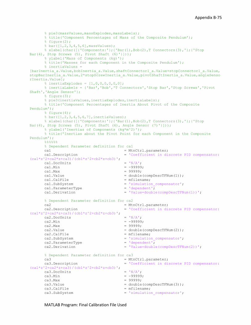
Appendix B-75
MATLAB Program: Final Calibration File Used
% pie3(massValues,massExplodes,massLabels);
% title('Component Percentages of Mass of the Composite Pendulum');
% figure(2);
% bar([1,2,3,4,5,6],massValues);
% xlabel(char([{'Components:'};{'Bar(1),Bob(2),T Connectors(3),'};{'Stop
Bar(4), Stop Screws (5), Pivot Shaft (6)'}]));
% ylabel('Mass of Components (kg)');
% title('Masses for each Component in the Composite Pendulum');
% inertiaValues =
[barInertia_a.Value,bobInertia_a.Value,shaftConnectorI_a.Value+stopConnectorI_a.Value,
stopBarInertia_a.Value,2*stopScrewInertia_a.Value,pivotShaftInertia_a.Value,angleSenso
rInertia.Value];
% inertiaExplodes = [1,0,0,0,0,0,0];
% inertiaLabels = {'Bar','Bob','T Connectors','Stop Bar','Stop Screws','Pivot
Shaft','Angle Sensor'};
% figure(3);
% pie3(inertiaValues,inertiaExplodes,inertiaLabels);
% title('Component Percentages of Inertia About Pivot of the Composite
Pendulum');
% figure(4);
% bar([1,2,3,4,5,6,7],inertiaValues);
% xlabel(char([{'Components:'};{'Bar(1),Bob(2),T Connectors(3),'};{'Stop
Bar(4), Stop Screws (5), Pivot Shaft (6), Angle Sensor (7)'}]));
% ylabel('Inertias of Components (kg*m^2)');
% title('Inertias about the Pivot Point for each Component in the Composite
Pendulum');
%%%%%%
% Dependent Parameter definition for ca1
ca1 = MtnCtrl.parameter;
ca1.Description = 'Coefficient in discrete PID compensator:
(ca1*z^2+ca2*z+ca3)/(cb1*z^2+cb2*z+cb3)';
ca1.DocUnits = 'N/A';
ca1.Min = -99999;
ca1.Max = 99999;
ca1.Value = double(compDescTFNum(1));
ca1.CalFile = mfilename;
ca1.SubSystem = 'simulation_compensator';
ca1.ParameterType = 'dependent';
ca1.Derivation = 'Value=double(compDescTFNum(1))';
% Dependent Parameter definition for ca2
ca2 = MtnCtrl.parameter;
ca2.Description = 'Coefficient in discrete PID compensator:
(ca1*z^2+ca2*z+ca3)/(cb1*z^2+cb2*z+cb3)';
ca2.DocUnits = 'N/A';
ca2.Min = -99999;
ca2.Max = 99999;
ca2.Value = double(compDescTFNum(2));
ca2.CalFile = mfilename;
ca2.SubSystem = 'simulation_compensator';
ca2.ParameterType = 'dependent';
ca2.Derivation = 'Value=double(compDescTFNum(2))';
% Dependent Parameter definition for ca3
ca3 = MtnCtrl.parameter;
ca3.Description = 'Coefficient in discrete PID compensator:
(ca1*z^2+ca2*z+ca3)/(cb1*z^2+cb2*z+cb3)';
ca3.DocUnits = 'N/A';
ca3.Min = -99999;
ca3.Max = 99999;
ca3.Value = double(compDescTFNum(3));
ca3.CalFile = mfilename;
ca3.SubSystem = 'simulation_compensator';
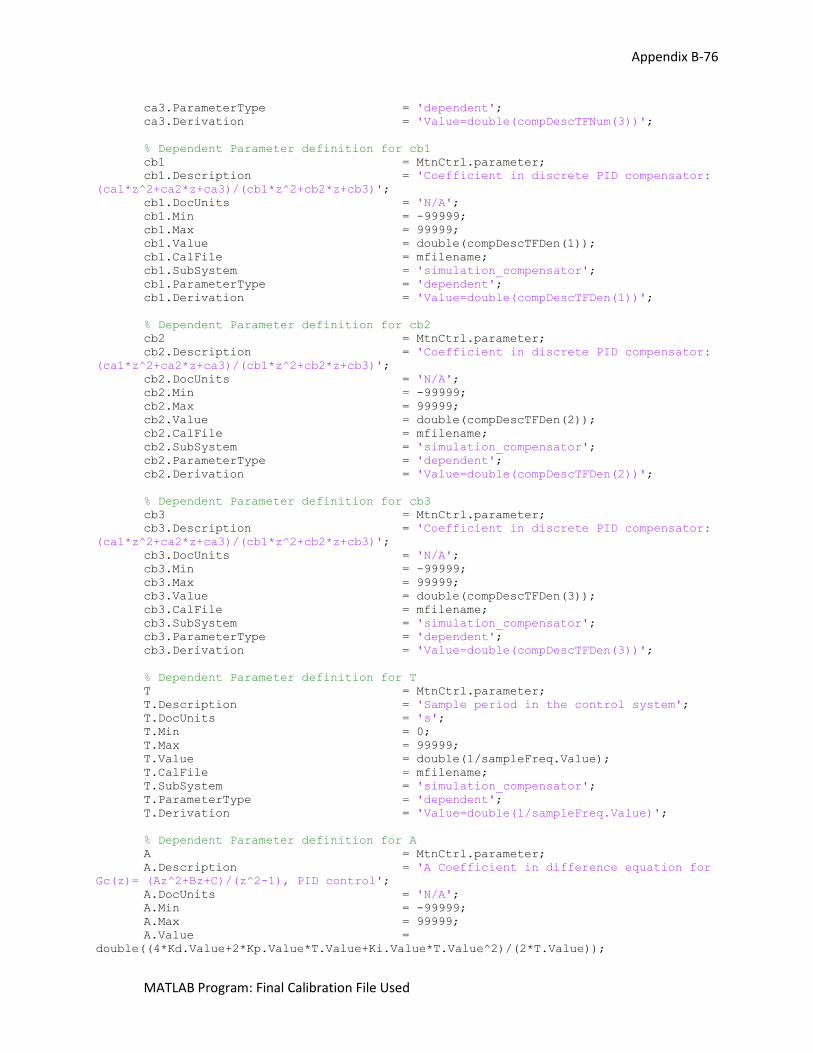
Appendix B-76
MATLAB Program: Final Calibration File Used
ca3.ParameterType = 'dependent';
ca3.Derivation = 'Value=double(compDescTFNum(3))';
% Dependent Parameter definition for cb1
cb1 = MtnCtrl.parameter;
cb1.Description = 'Coefficient in discrete PID compensator:
(ca1*z^2+ca2*z+ca3)/(cb1*z^2+cb2*z+cb3)';
cb1.DocUnits = 'N/A';
cb1.Min = -99999;
cb1.Max = 99999;
cb1.Value = double(compDescTFDen(1));
cb1.CalFile = mfilename;
cb1.SubSystem = 'simulation_compensator';
cb1.ParameterType = 'dependent';
cb1.Derivation = 'Value=double(compDescTFDen(1))';
% Dependent Parameter definition for cb2
cb2 = MtnCtrl.parameter;
cb2.Description = 'Coefficient in discrete PID compensator:
(ca1*z^2+ca2*z+ca3)/(cb1*z^2+cb2*z+cb3)';
cb2.DocUnits = 'N/A';
cb2.Min = -99999;
cb2.Max = 99999;
cb2.Value = double(compDescTFDen(2));
cb2.CalFile = mfilename;
cb2.SubSystem = 'simulation_compensator';
cb2.ParameterType = 'dependent';
cb2.Derivation = 'Value=double(compDescTFDen(2))';
% Dependent Parameter definition for cb3
cb3 = MtnCtrl.parameter;
cb3.Description = 'Coefficient in discrete PID compensator:
(ca1*z^2+ca2*z+ca3)/(cb1*z^2+cb2*z+cb3)';
cb3.DocUnits = 'N/A';
cb3.Min = -99999;
cb3.Max = 99999;
cb3.Value = double(compDescTFDen(3));
cb3.CalFile = mfilename;
cb3.SubSystem = 'simulation_compensator';
cb3.ParameterType = 'dependent';
cb3.Derivation = 'Value=double(compDescTFDen(3))';
% Dependent Parameter definition for T
T = MtnCtrl.parameter;
T.Description = 'Sample period in the control system';
T.DocUnits = 's';
T.Min = 0;
T.Max = 99999;
T.Value = double(1/sampleFreq.Value);
T.CalFile = mfilename;
T.SubSystem = 'simulation_compensator';
T.ParameterType = 'dependent';
T.Derivation = 'Value=double(1/sampleFreq.Value)';
% Dependent Parameter definition for A
A = MtnCtrl.parameter;
A.Description = 'A Coefficient in difference equation for
Gc(z)= (Az^2+Bz+C)/(z^2-1), PID control';
A.DocUnits = 'N/A';
A.Min = -99999;
A.Max = 99999;
A.Value =
double((4*Kd.Value+2*Kp.Value*T.Value+Ki.Value*T.Value^2)/(2*T.Value));
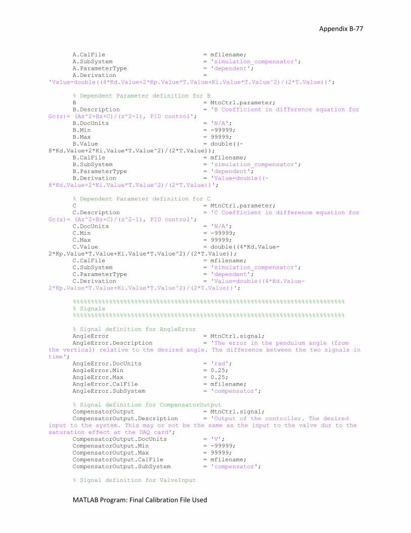
Appendix B-77
MATLAB Program: Final Calibration File Used
A.CalFile = mfilename;
A.SubSystem = 'simulation_compensator';
A.ParameterType = 'dependent';
A.Derivation =
'Value=double((4*Kd.Value+2*Kp.Value*T.Value+Ki.Value*T.Value^2)/(2*T.Value))';
% Dependent Parameter definition for B
B = MtnCtrl.parameter;
B.Description = 'B Coefficient in difference equation for
Gc(z)= (Az^2+Bz+C)/(z^2-1), PID control';
B.DocUnits = 'N/A';
B.Min = -99999;
B.Max = 99999;
B.Value = double((-
8*Kd.Value+2*Ki.Value*T.Value^2)/(2*T.Value));
B.CalFile = mfilename;
B.SubSystem = 'simulation_compensator';
B.ParameterType = 'dependent';
B.Derivation = 'Value=double((-
8*Kd.Value+2*Ki.Value*T.Value^2)/(2*T.Value))';
% Dependent Parameter definition for C
C = MtnCtrl.parameter;
C.Description = 'C Coefficient in difference equation for
Gc(z)= (Az^2+Bz+C)/(z^2-1), PID control';
C.DocUnits = 'N/A';
C.Min = -99999;
C.Max = 99999;
C.Value = double((4*Kd.Value-
2*Kp.Value*T.Value+Ki.Value*T.Value^2)/(2*T.Value));
C.CalFile = mfilename;
C.SubSystem = 'simulation_compensator';
C.ParameterType = 'dependent';
C.Derivation = 'Value=double((4*Kd.Value-
2*Kp.Value*T.Value+Ki.Value*T.Value^2)/(2*T.Value))';
%%%%%%%%%%%%%%%%%%%%%%%%%%%%%%%%%%%%%%%%%%%%%%%%%%%%%%%%%%%%%%%%%%%%%%%%%%%
% Signals
%%%%%%%%%%%%%%%%%%%%%%%%%%%%%%%%%%%%%%%%%%%%%%%%%%%%%%%%%%%%%%%%%%%%%%%%%%%
% Signal definition for AngleError
AngleError = MtnCtrl.signal;
AngleError.Description = 'The error in the pendulum angle (from
the vertical) relative to the desired angle. The difference between the two signals in
time';
AngleError.DocUnits = 'rad';
AngleError.Min = 0.25;
AngleError.Max = 0.25;
AngleError.CalFile = mfilename;
AngleError.SubSystem = 'compensator';
% Signal definition for CompensatorOutput
CompensatorOutput = MtnCtrl.signal;
CompensatorOutput.Description = 'Output of the controller. The desired
input to the system. This may or not be the same as the input to the valve dur to the
saturation effect at the DAQ card';
CompensatorOutput.DocUnits = 'V';
CompensatorOutput.Min = -99999;
CompensatorOutput.Max = 99999;
CompensatorOutput.CalFile = mfilename;
CompensatorOutput.SubSystem = 'compensator';
% Signal definition for ValveInput
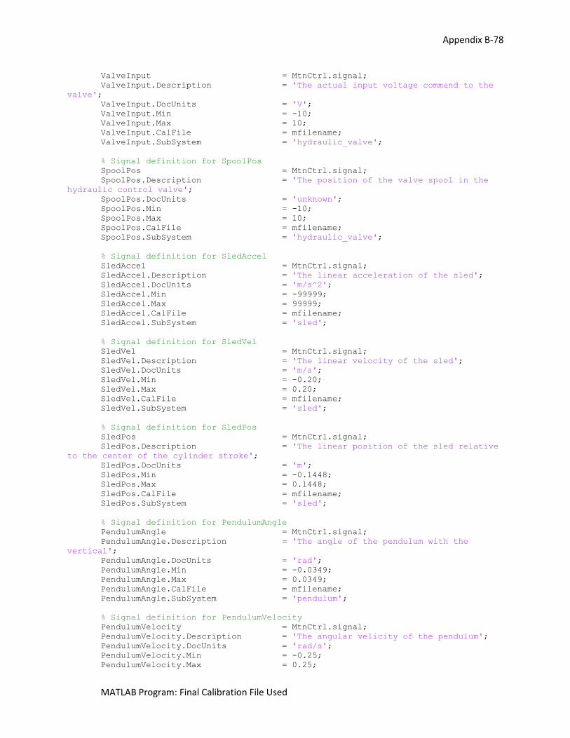
Appendix B-78
MATLAB Program: Final Calibration File Used
ValveInput = MtnCtrl.signal;
ValveInput.Description = 'The actual input voltage command to the
valve';
ValveInput.DocUnits = 'V';
ValveInput.Min = -10;
ValveInput.Max = 10;
ValveInput.CalFile = mfilename;
ValveInput.SubSystem = 'hydraulic_valve';
% Signal definition for SpoolPos
SpoolPos = MtnCtrl.signal;
SpoolPos.Description = 'The position of the valve spool in the
hydraulic control valve';
SpoolPos.DocUnits = 'unknown';
SpoolPos.Min = -10;
SpoolPos.Max = 10;
SpoolPos.CalFile = mfilename;
SpoolPos.SubSystem = 'hydraulic_valve';
% Signal definition for SledAccel
SledAccel = MtnCtrl.signal;
SledAccel.Description = 'The linear acceleration of the sled';
SledAccel.DocUnits = 'm/s^2';
SledAccel.Min = -99999;
SledAccel.Max = 99999;
SledAccel.CalFile = mfilename;
SledAccel.SubSystem = 'sled';
% Signal definition for SledVel
SledVel = MtnCtrl.signal;
SledVel.Description = 'The linear velocity of the sled';
SledVel.DocUnits = 'm/s';
SledVel.Min = -0.20;
SledVel.Max = 0.20;
SledVel.CalFile = mfilename;
SledVel.SubSystem = 'sled';
% Signal definition for SledPos
SledPos = MtnCtrl.signal;
SledPos.Description = 'The linear position of the sled relative
to the center of the cylinder stroke';
SledPos.DocUnits = 'm';
SledPos.Min = -0.1448;
SledPos.Max = 0.1448;
SledPos.CalFile = mfilename;
SledPos.SubSystem = 'sled';
% Signal definition for PendulumAngle
PendulumAngle = MtnCtrl.signal;
PendulumAngle.Description = 'The angle of the pendulum with the
vertical';
PendulumAngle.DocUnits = 'rad';
PendulumAngle.Min = -0.0349;
PendulumAngle.Max = 0.0349;
PendulumAngle.CalFile = mfilename;
PendulumAngle.SubSystem = 'pendulum';
% Signal definition for PendulumVelocity
PendulumVelocity = MtnCtrl.signal;
PendulumVelocity.Description = 'The angular velicity of the pendulum';
PendulumVelocity.DocUnits = 'rad/s';
PendulumVelocity.Min = -0.25;
PendulumVelocity.Max = 0.25;

Appendix B-79
MATLAB Program: Final Calibration File Used
PendulumVelocity.CalFile = mfilename;
PendulumVelocity.SubSystem = 'pendulum';
% package calibrations into calibrationStruct structure
calibrations = whos;
for var = 1:length(calibrations)
calibrationStruct.(calibrations(var).name) = eval(calibrations(var).name);
end
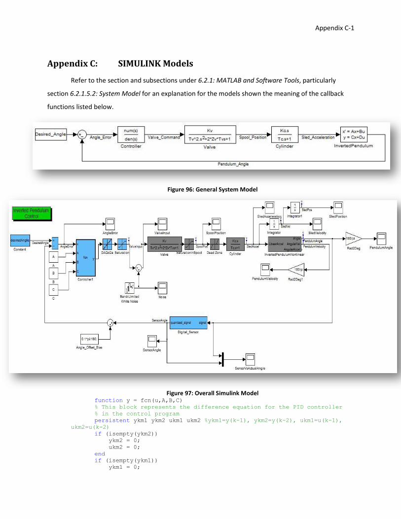
Appendix C-1
Appendix C: SIMULINK Models
Refer to the section and subsections under 6.2.1: MATLAB and Software Tools, particularly
section 6.2.1.5.2: System Model for an explanation for the models shown the meaning of the callback
functions listed below.
Figure 96: General System Model
Figure 97: Overall Simulink Model
function y = fcn(u,A,B,C)
% This block represents the difference equation for the PID controller
% in the control program
persistent ykm1 ykm2 ukm1 ukm2 %ykm1=y(k-1), ykm2=y(k-2), ukm1=u(k-1),
ukm2=u(k-2)
if (isempty(ykm2))
ykm2 = 0;
ukm2 = 0;
end
if (isempty(ykm1))
ykm1 = 0;
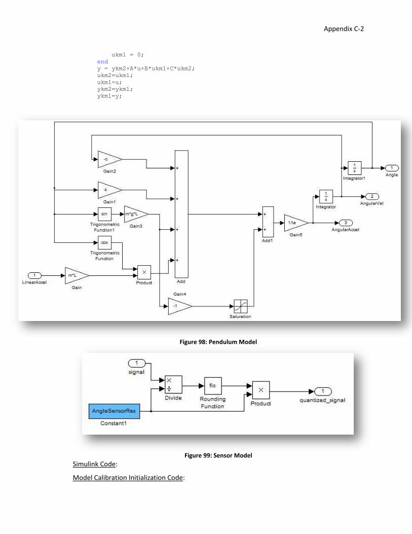
Appendix C-2
ukm1 = 0;
end
y = ykm2+A*u+B*ukm1+C*ukm2;
ukm2=ukm1;
ukm1=u;
ykm2=ykm1;
ykm1=y;
Figure 98: Pendulum Model
Figure 99: Sensor Model
Simulink Code:
Model Calibration Initialization Code:

Appendix C-3
clear all modelNameToBeInitialized = '<model name>'; [calibrations, calibrationFileInitializedFrom] = getCalibrationSet(modelNameToBeInitialized); fieldNamesInCalibrations = fieldnames(calibrations); for i = 1:length(fieldNamesInCalibrations) eval([fieldNamesInCalibrations{i} ' = calibrations.(fieldNamesInCalibrations{i});']); end clear i calibrations fieldNamesInCalibrations modelNameToBeInitialized StopFcn Callback: modelName = '<model name>'; graphResults(modelName ); getPerformanceResults(modelName); PreSaveFcn Callback: modelName = '<model name>'; closeScopes(modelName);
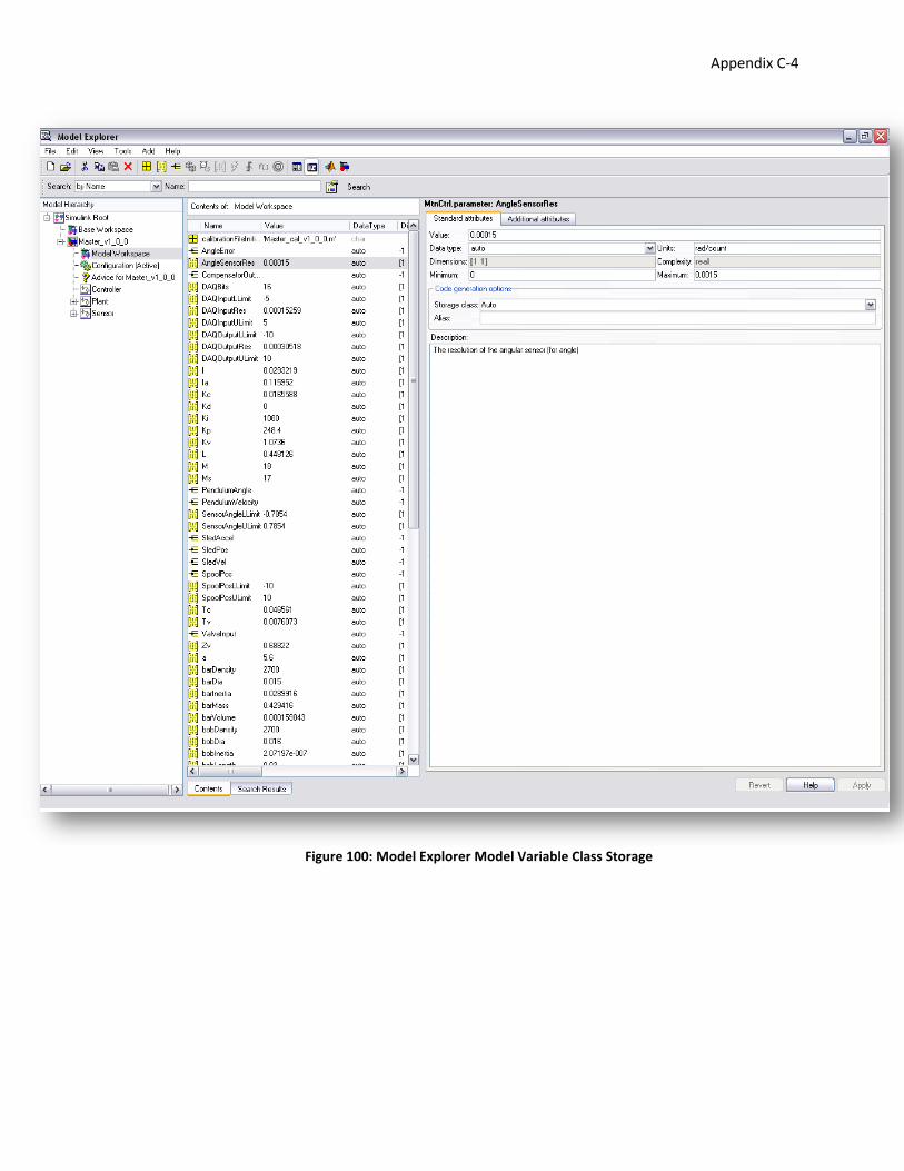
Appendix C-4
Figure 100: Model Explorer Model Variable Class Storage
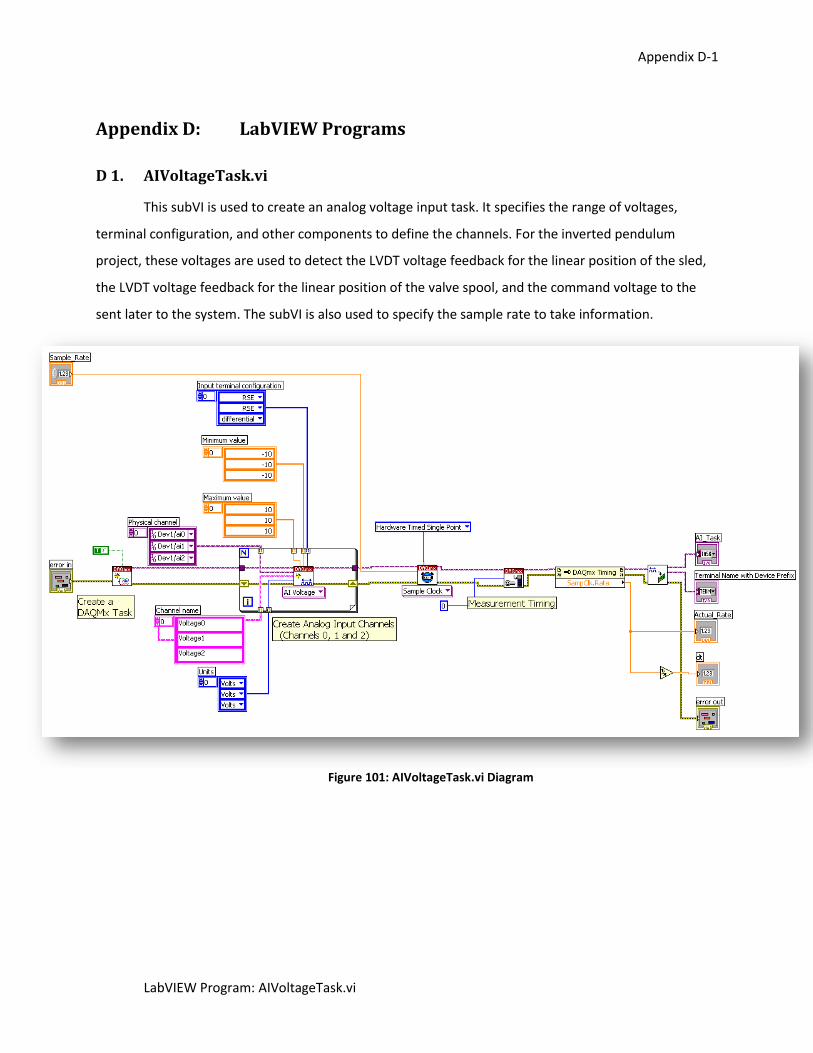
Appendix D-1
LabVIEW Program: AIVoltageTask.vi
Appendix D: LabVIEW Programs
D 1. AIVoltageTask.vi
This subVI is used to create an analog voltage input task. It specifies the range of voltages,
terminal configuration, and other components to define the channels. For the inverted pendulum
project, these voltages are used to detect the LVDT voltage feedback for the linear position of the sled,
the LVDT voltage feedback for the linear position of the valve spool, and the command voltage to the
sent later to the system. The subVI is also used to specify the sample rate to take information.
Figure 101: AIVoltageTask.vi Diagram
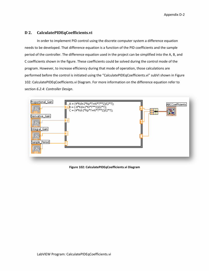
Appendix D-2
LabVIEW Program: CalculatePIDEqCoefficients.vi
D 2. CalculatePIDEqCoefficients.vi
In order to implement PID control using the discrete computer system a difference equation
needs to be developed. That difference equation is a function of the PID coefficients and the sample
period of the controller. The difference equation used in the project can be simplified into the A, B, and
C coefficients shown in the figure. These coefficients could be solved during the control mode of the
program. However, to increase efficiency during that mode of operation, those calculations are
performed before the control is initiated using the “CalculatePIDEqCoefficients.vi” subVI shown in Figure
102: CalculatePIDEqCoefficients.vi Diagram. For more information on the difference equation refer to
section 6.2.4: Controller Design.
Figure 102: CalculatePIDEqCoefficients.vi Diagram
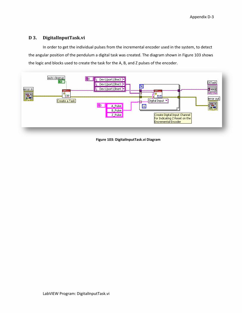
Appendix D-3
LabVIEW Program: DigitalInputTask.vi
D 3. DigitalInputTask.vi
In order to get the individual pulses from the incremental encoder used in the system, to detect
the angular position of the pendulum a digital task was created. The diagram shown in Figure 103 shows
the logic and blocks used to create the task for the A, B, and Z pulses of the encoder.
Figure 103: DigitalInputTask.vi Diagram
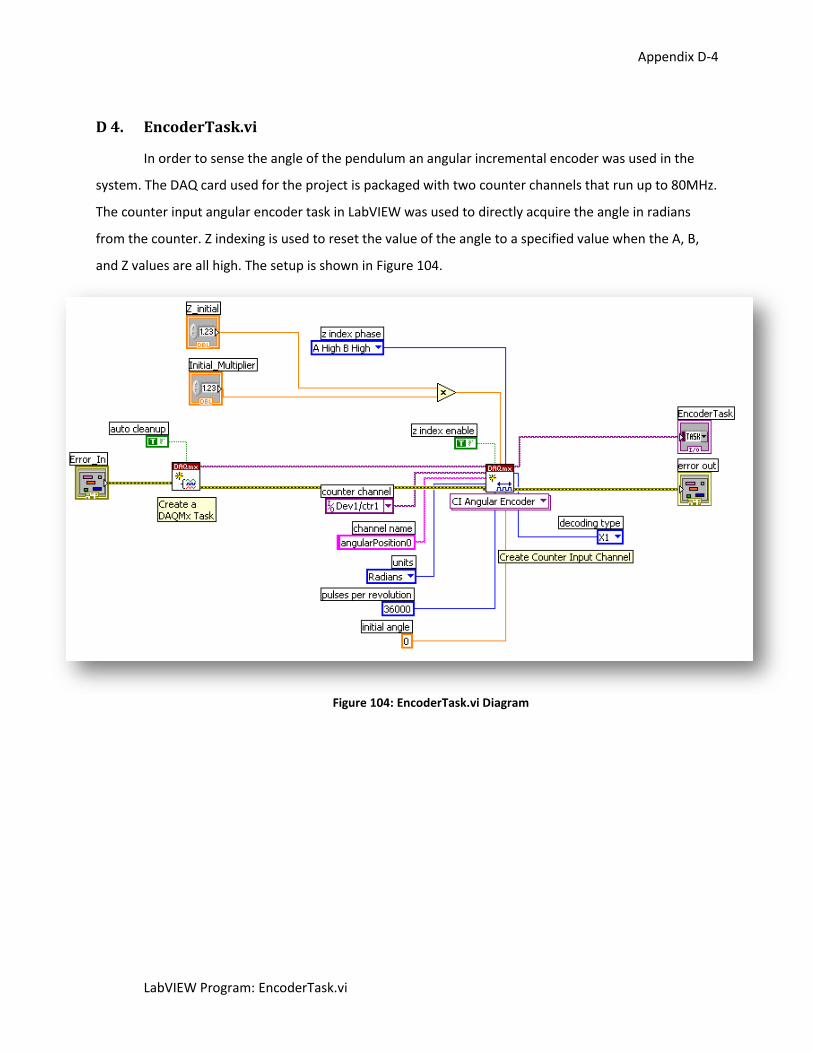
Appendix D-4
LabVIEW Program: EncoderTask.vi
D 4. EncoderTask.vi
In order to sense the angle of the pendulum an angular incremental encoder was used in the
system. The DAQ card used for the project is packaged with two counter channels that run up to 80MHz.
The counter input angular encoder task in LabVIEW was used to directly acquire the angle in radians
from the counter. Z indexing is used to reset the value of the angle to a specified value when the A, B,
and Z values are all high. The setup is shown in Figure 104.
Figure 104: EncoderTask.vi Diagram
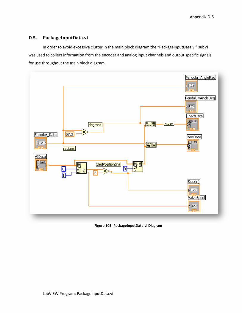
Appendix D-5
LabVIEW Program: PackageInputData.vi
D 5. PackageInputData.vi
In order to avoid excessive clutter in the main block diagram the “PackageInputData.vi” subVI
was used to collect information from the encoder and analog input channels and output specific signals
for use throughout the main block diagram.
Figure 105: PackageInputData.vi Diagram
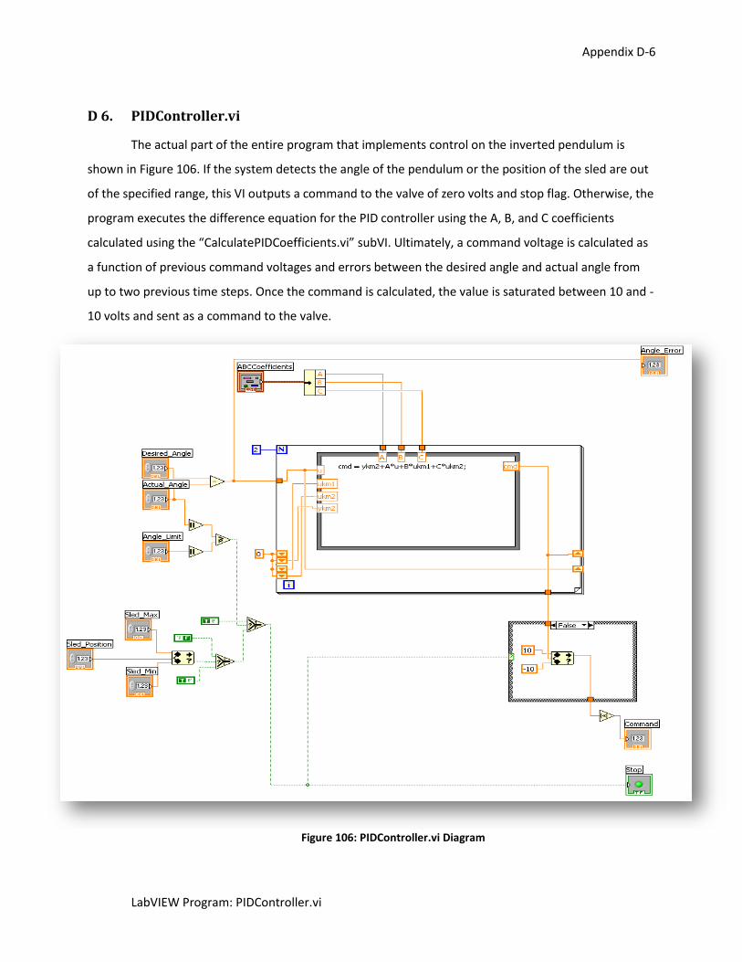
Appendix D-6
LabVIEW Program: PIDController.vi
D 6. PIDController.vi
The actual part of the entire program that implements control on the inverted pendulum is
shown in Figure 106. If the system detects the angle of the pendulum or the position of the sled are out
of the specified range, this VI outputs a command to the valve of zero volts and stop flag. Otherwise, the
program executes the difference equation for the PID controller using the A, B, and C coefficients
calculated using the “CalculatePIDCoefficients.vi” subVI. Ultimately, a command voltage is calculated as
a function of previous command voltages and errors between the desired angle and actual angle from
up to two previous time steps. Once the command is calculated, the value is saturated between 10 and -
10 volts and sent as a command to the valve.
Figure 106: PIDController.vi Diagram
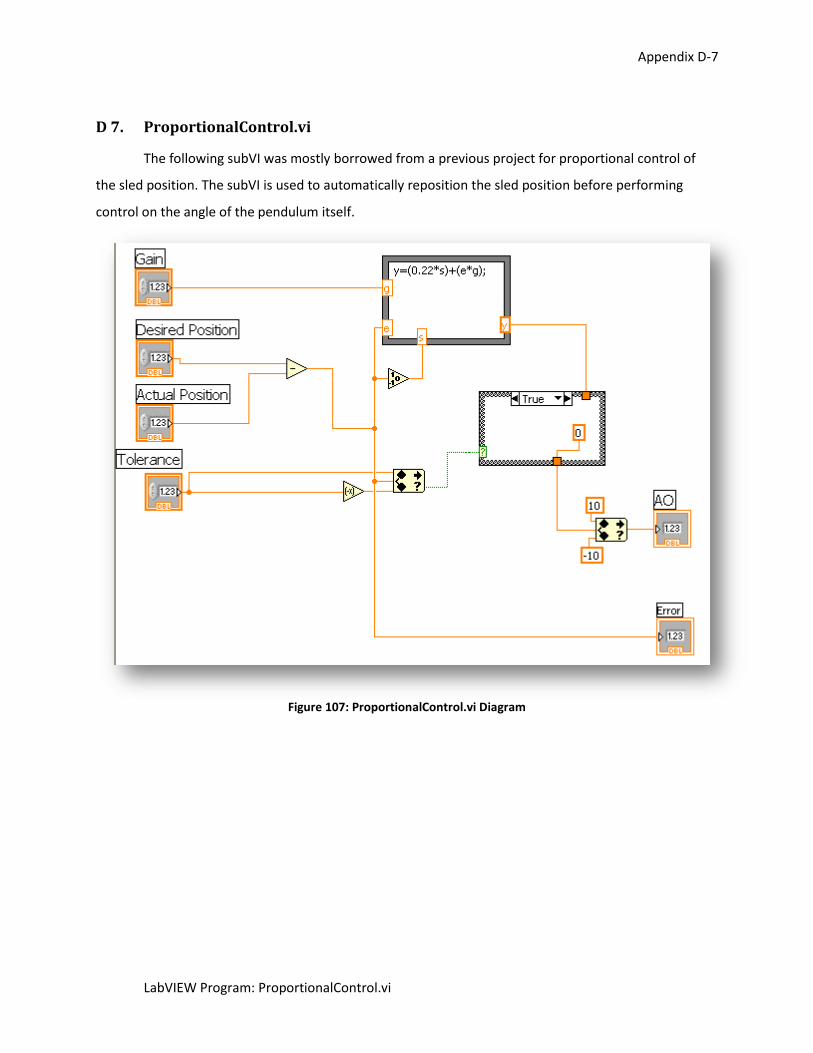
Appendix D-7
LabVIEW Program: ProportionalControl.vi
D 7. ProportionalControl.vi
The following subVI was mostly borrowed from a previous project for proportional control of
the sled position. The subVI is used to automatically reposition the sled position before performing
control on the angle of the pendulum itself.
Figure 107: ProportionalControl.vi Diagram
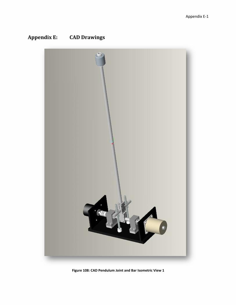
Appendix E-1
Appendix E: CAD Drawings
Figure 108: CAD Pendulum Joint and Bar Isometric View 1
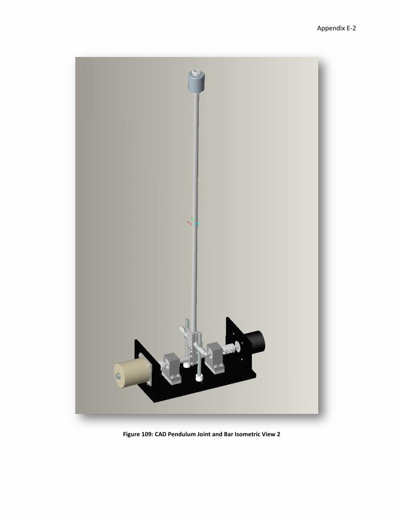
Appendix E-2
Figure 109: CAD Pendulum Joint and Bar Isometric View 2
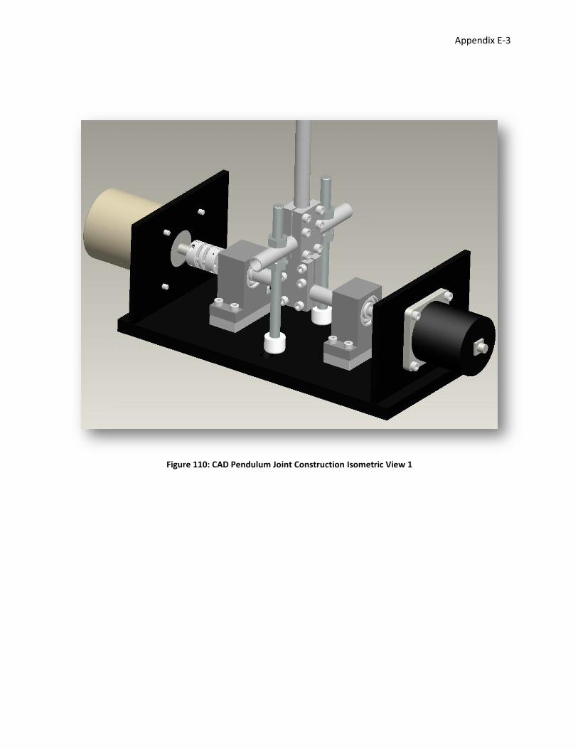
Appendix E-3
Figure 110: CAD Pendulum Joint Construction Isometric View 1
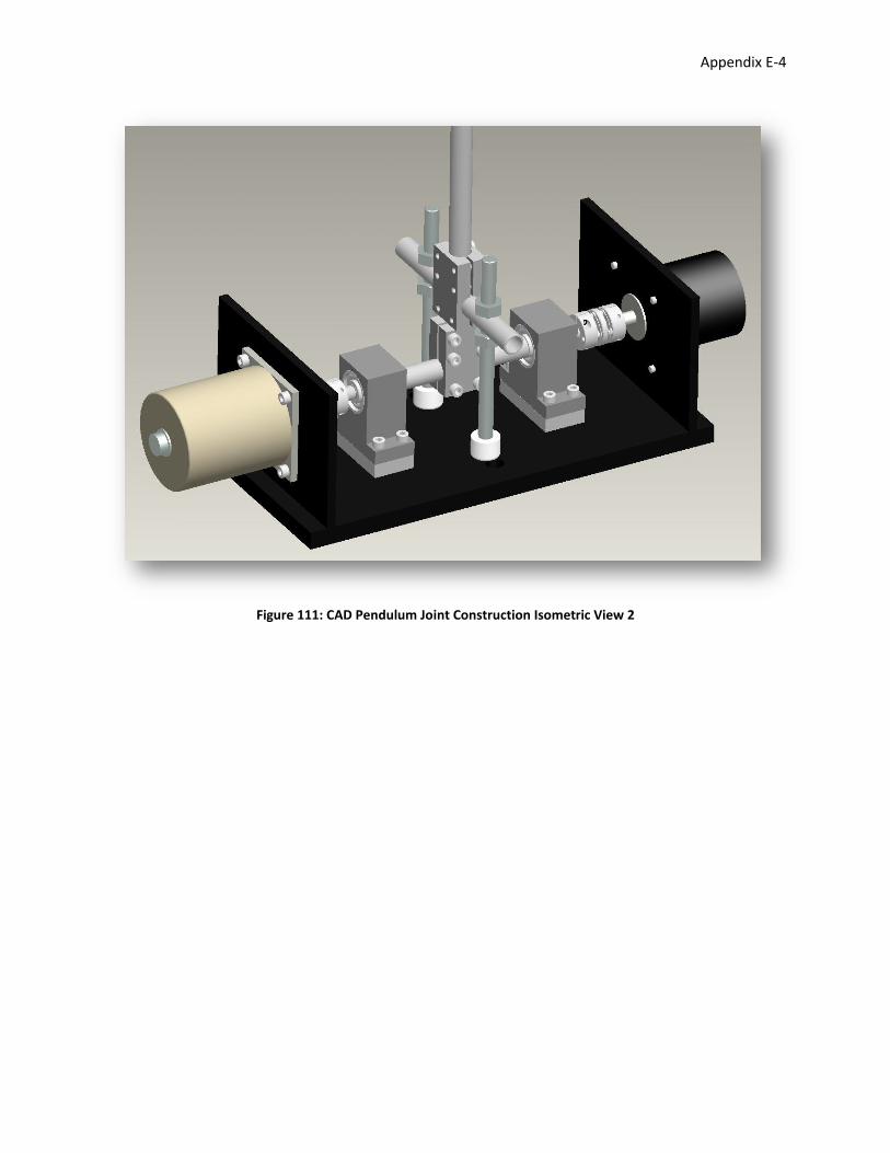
Appendix E-4
Figure 111: CAD Pendulum Joint Construction Isometric View 2
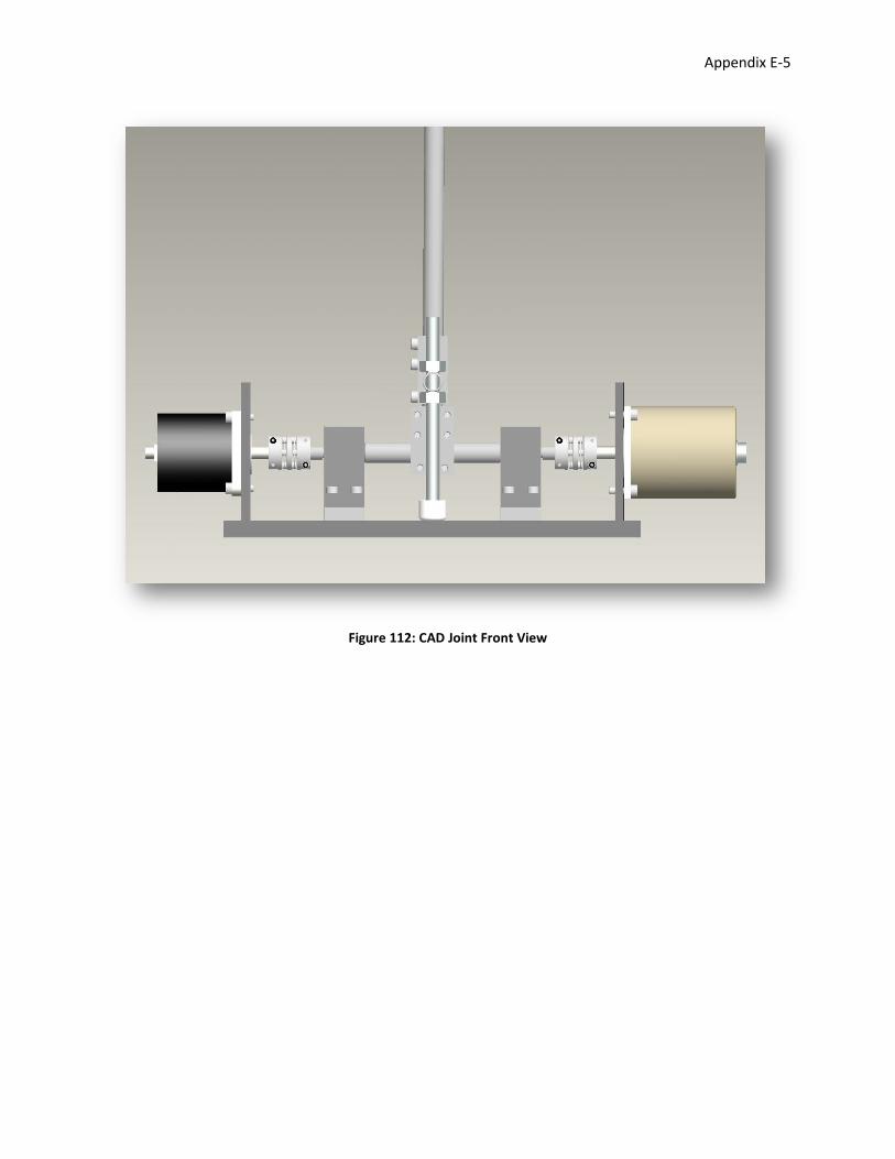
Appendix E-5
Figure 112: CAD Joint Front View
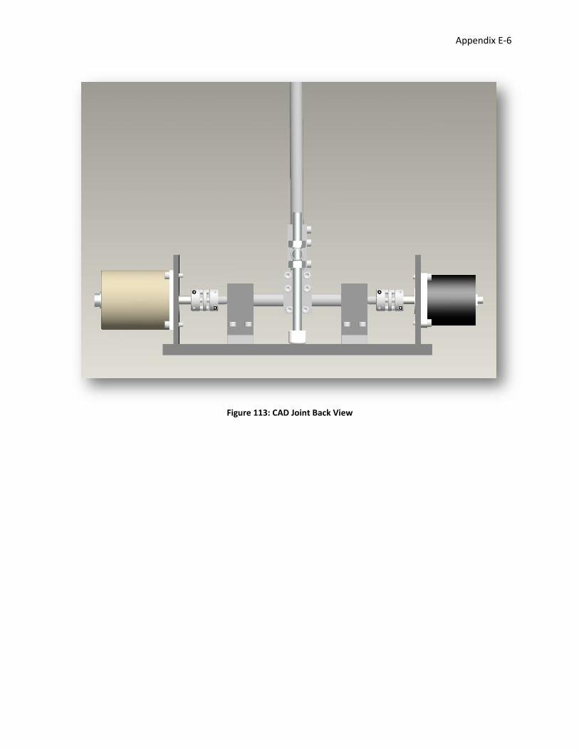
Appendix E-6
Figure 113: CAD Joint Back View
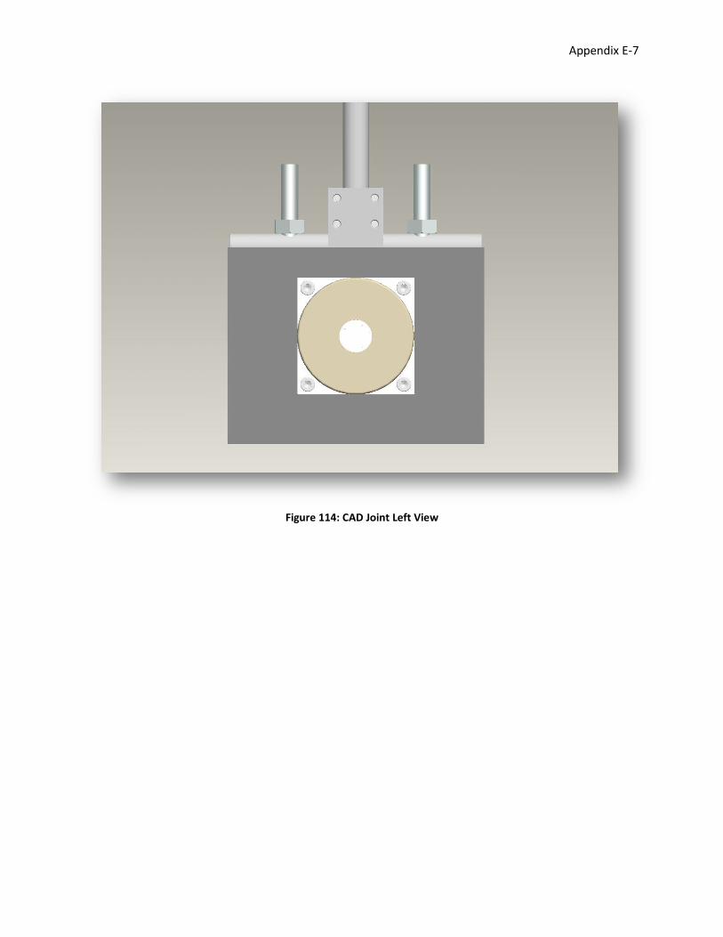
Appendix E-7
Figure 114: CAD Joint Left View
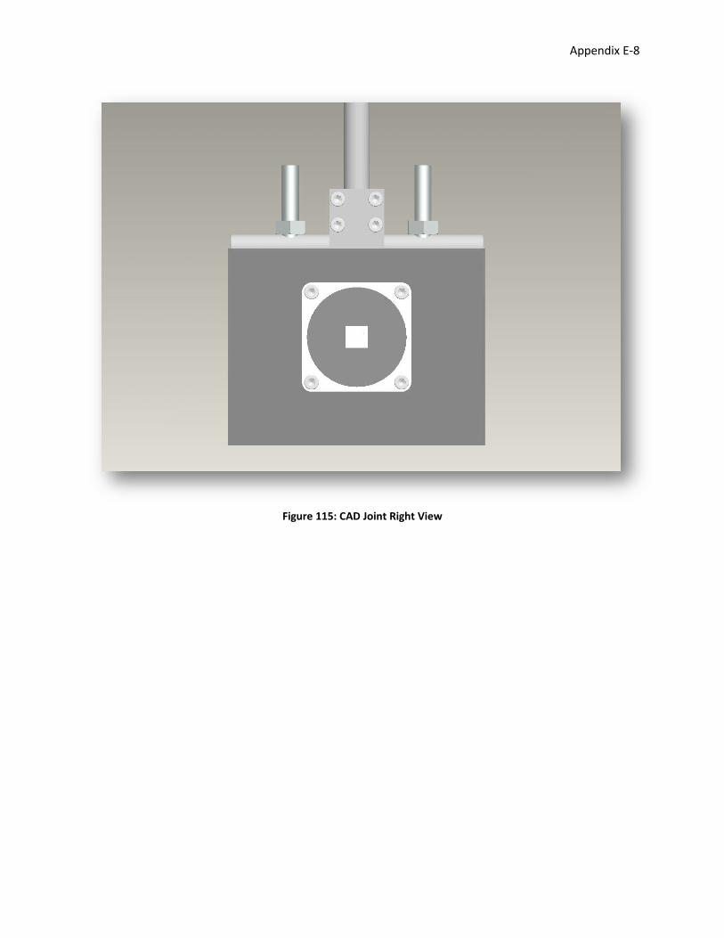
Appendix E-8
Figure 115: CAD Joint Right View
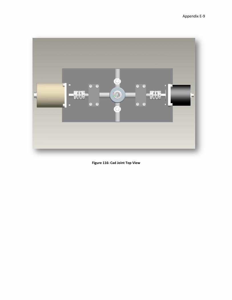
Appendix E-9
Figure 116: Cad Joint Top View
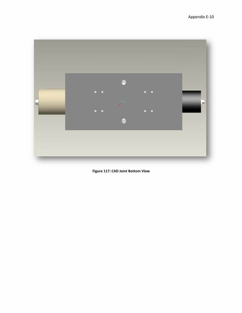
Appendix E-10
Figure 117: CAD Joint Bottom View
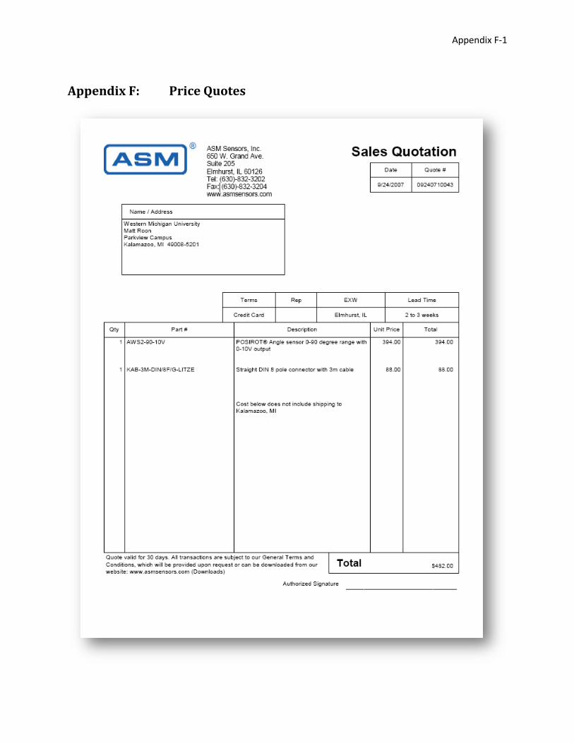
Appendix F-1
Appendix F: Price Quotes
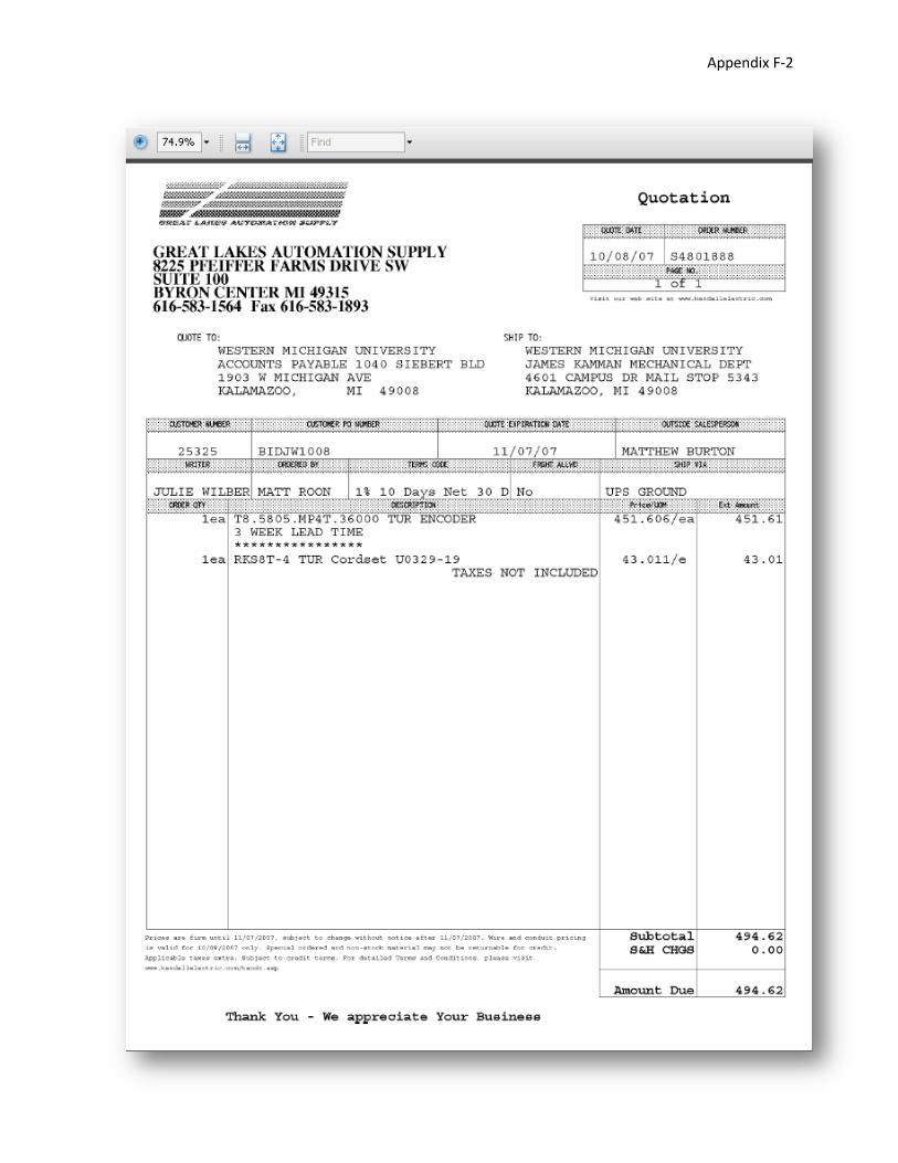
Appendix F-2
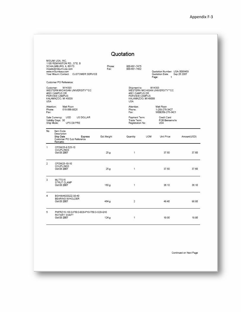
Appendix F-3
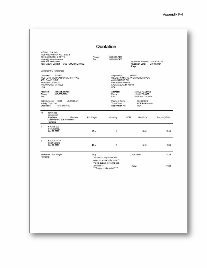
Appendix F-4
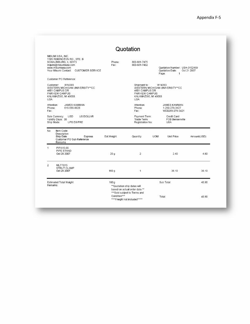
Appendix F-5
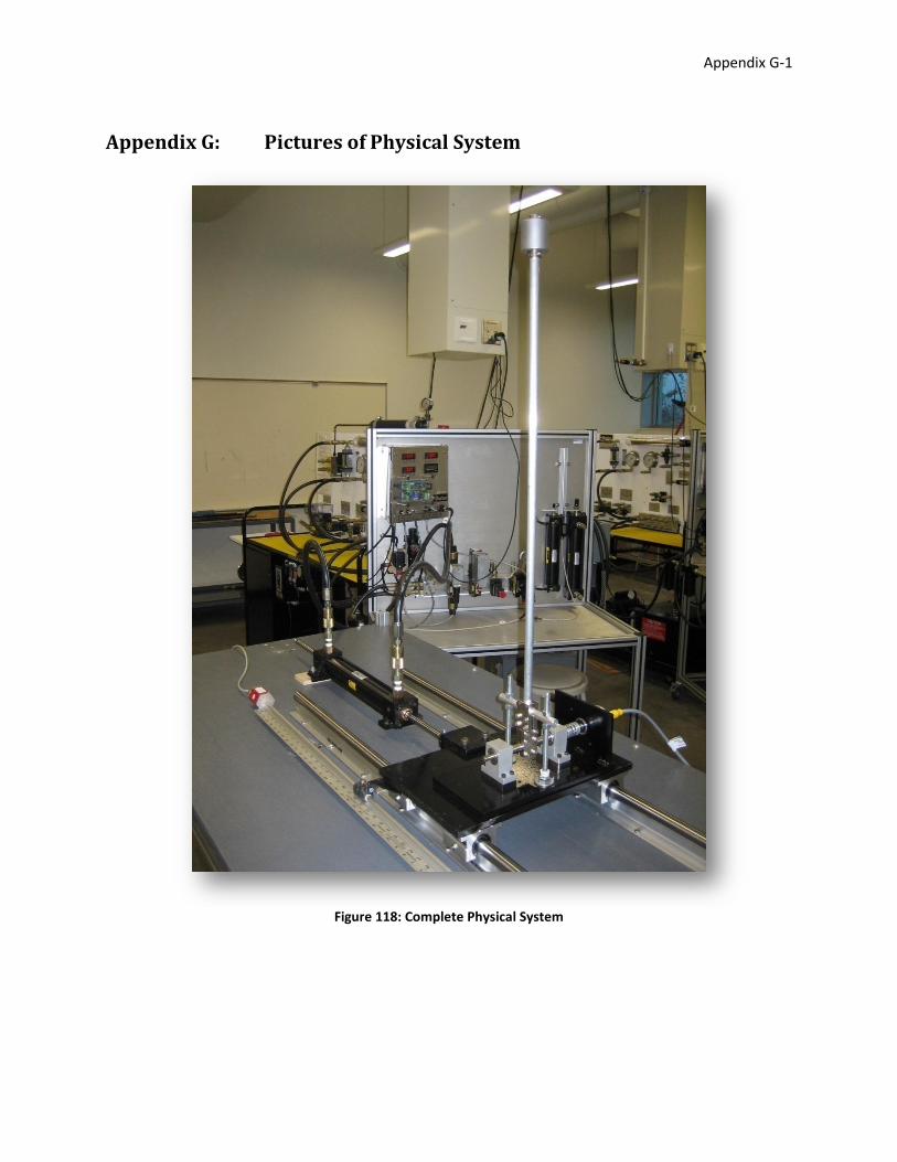
Appendix G-1
Appendix G: Pictures of Physical System
Figure 118: Complete Physical System
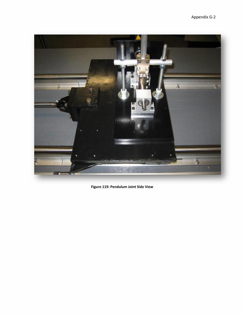
Appendix G-2
Figure 119: Pendulum Joint Side View
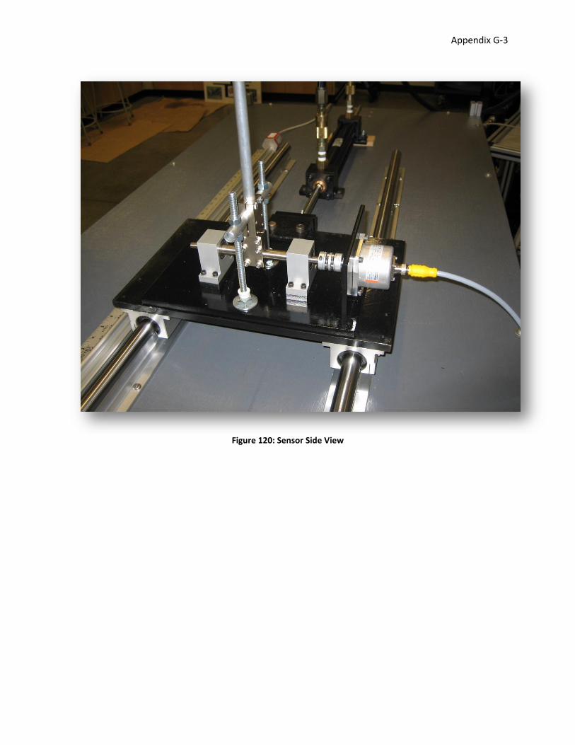
Appendix G-3
Figure 120: Sensor Side View
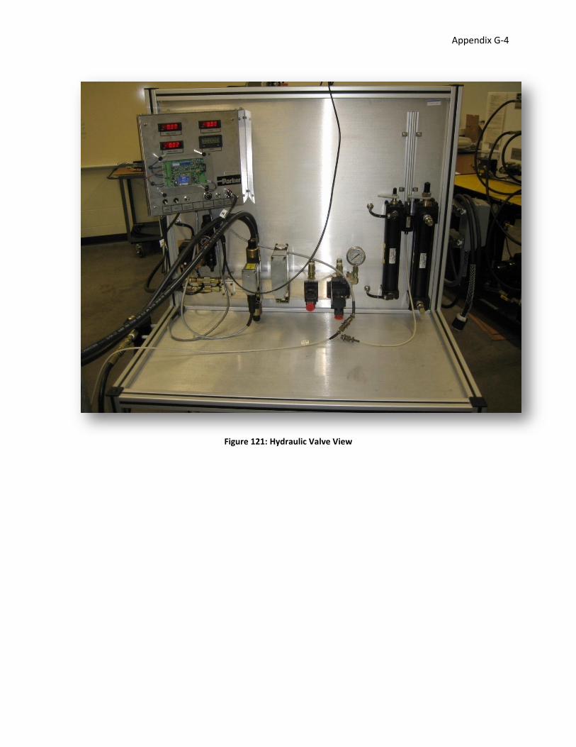
Appendix G-4
Figure 121: Hydraulic Valve View
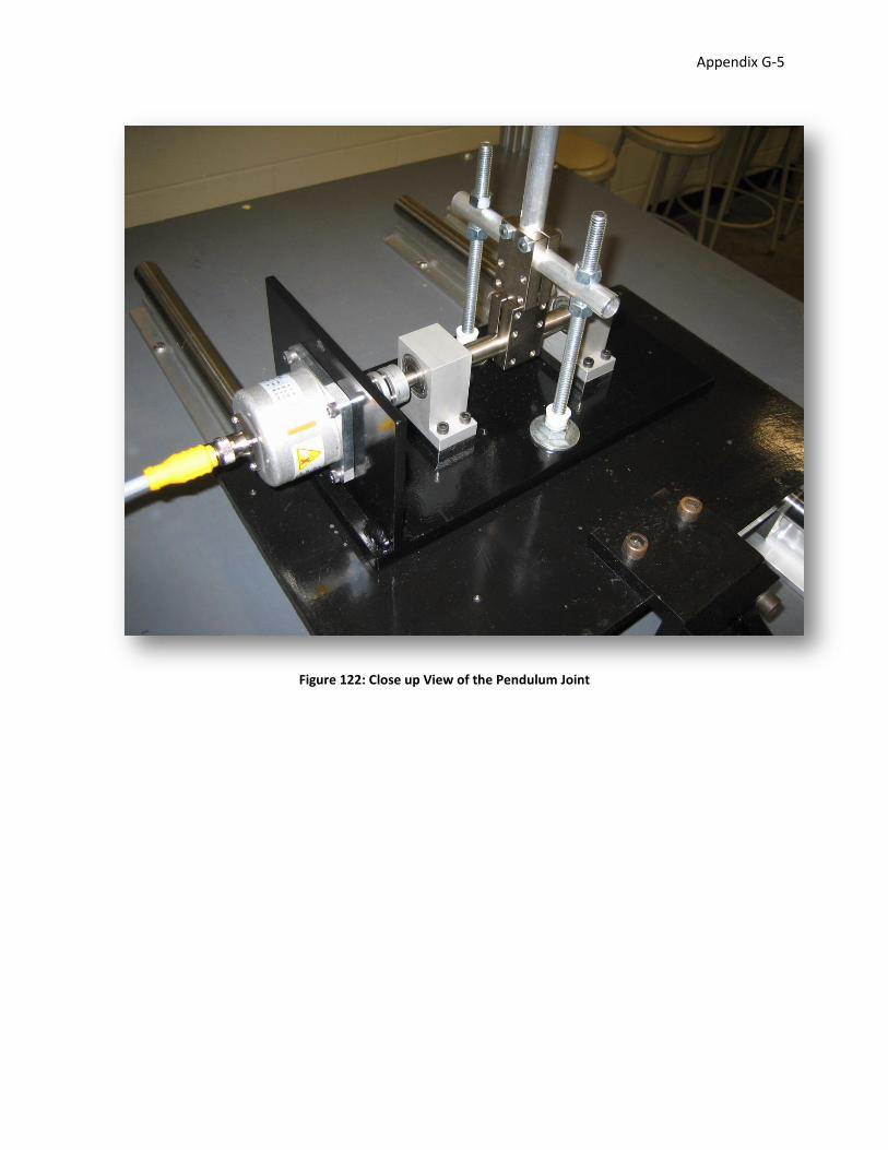
Appendix G-5
Figure 122: Close up View of the Pendulum Joint
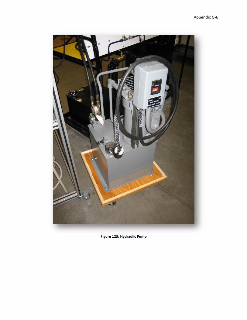
Appendix G-6
Figure 123: Hydraulic Pump
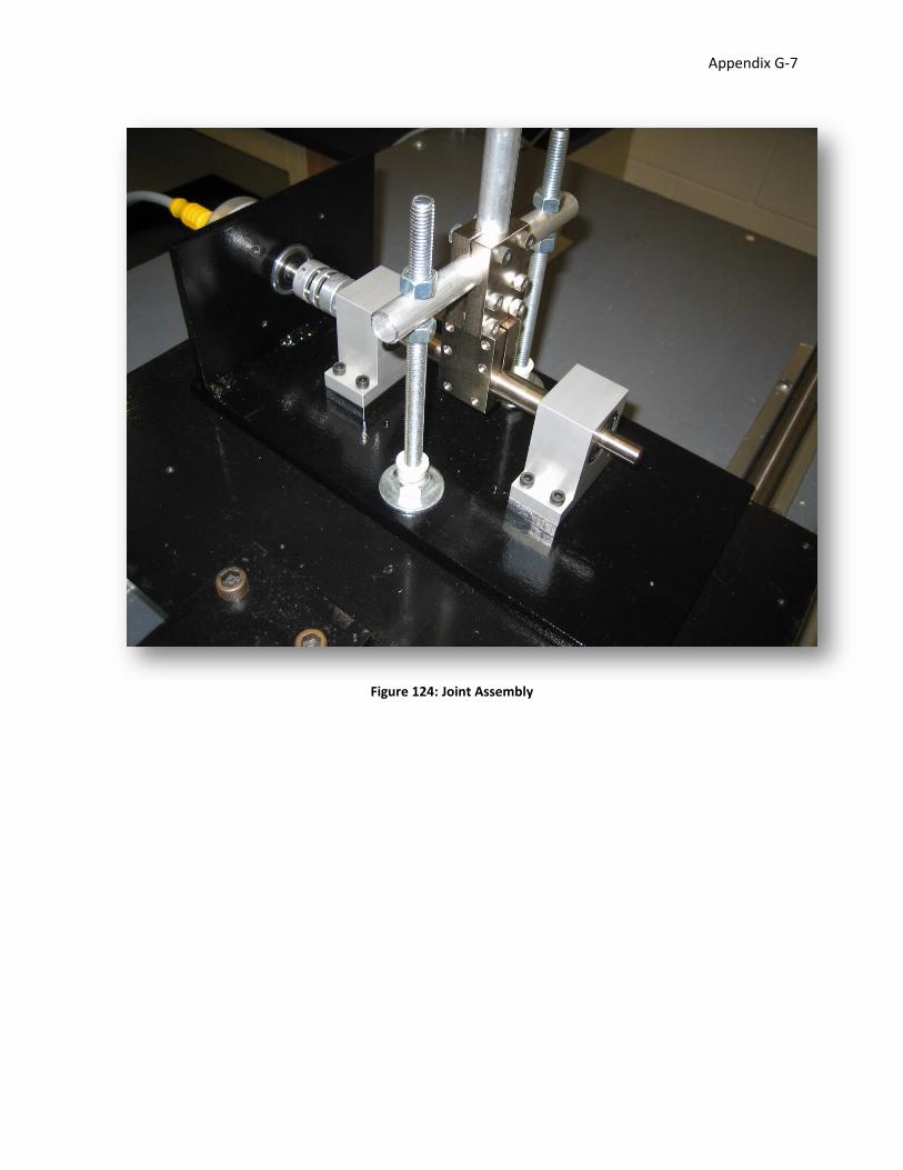
Appendix G-7
Figure 124: Joint Assembly
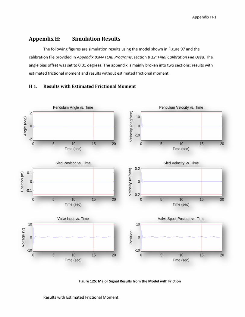
Appendix H-1
Results with Estimated Frictional Moment
Appendix H: Simulation Results
The following figures are simulation results using the model shown in Figure 97 and the
calibration file provided in Appendix B:MATLAB Programs, section B 12: Final Calibration File Used. The
angle bias offset was set to 0.01 degrees. The appendix is mainly broken into two sections: results with
estimated frictional moment and results without estimated frictional moment.
H 1. Results with Estimated Frictional Moment
Figure 125: Major Signal Results from the Model with Friction
0 5 10 15 20
-2
0
2
Pendulum Angle vs. Time
Time (sec)
Angle
(deg)
0 5 10 15 20
-10
0
10
Pendulum Velocity vs. Time
Time (sec)
Velo
city (
deg/s
ec)
0 5 10 15 20
-0.1
0
0.1
Sled Position vs. Time
Time (sec)
Positio
n (
m)
0 5 10 15 20
-0.2
0
0.2
Sled Velocity vs. Time
Time (sec)
Velo
city (
m/s
ec)
0 5 10 15 20
-10
0
10
Valve Input vs. Time
Time (sec)
Voltage (
V)
0 5 10 15 20
-10
0
10
Valve Spool Position vs. Time
Time (sec)
Positio
n
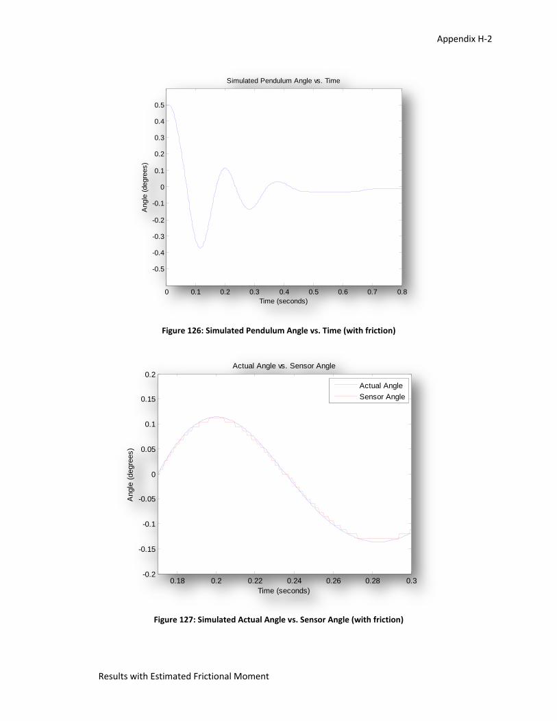
Appendix H-2
Results with Estimated Frictional Moment
Figure 126: Simulated Pendulum Angle vs. Time (with friction)
Figure 127: Simulated Actual Angle vs. Sensor Angle (with friction)
0 0.1 0.2 0.3 0.4 0.5 0.6 0.7 0.8
-0.5
-0.4
-0.3
-0.2
-0.1
0
0.1
0.2
0.3
0.4
0.5
Simulated Pendulum Angle vs. Time
Time (seconds)
Angle
(degre
es)
0.18 0.2 0.22 0.24 0.26 0.28 0.3-0.2
-0.15
-0.1
-0.05
0
0.05
0.1
0.15
0.2Actual Angle vs. Sensor Angle
Time (seconds)
Angle
(degre
es)
Actual Angle
Sensor Angle
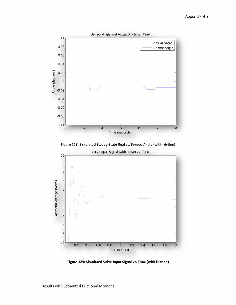
Appendix H-3
Results with Estimated Frictional Moment
Figure 128: Simulated Steady-State Real vs. Sensed Angle (with friction)
Figure 129: Simulated Valve Input Signal vs. Time (with friction)
2 3 4 5 6 7 8-0.1
-0.08
-0.06
-0.04
-0.02
0
0.02
0.04
0.06
0.08
0.1Sensor Angle and Actual Angle vs. Time
Time (seconds)
Angle
(degre
es)
Actual Angle
Sensor Angle
0 0.2 0.4 0.6 0.8 1 1.2 1.4 1.6 1.8 2-10
-8
-6
-4
-2
0
2
4
6
8
10Valve Input Signal (with noise) vs. Time
Time (seconds)
Com
mand V
oltage (
Volts)
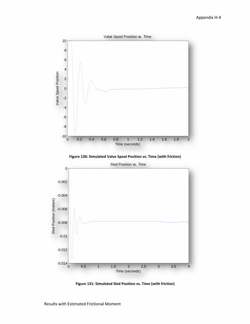
Appendix H-4
Results with Estimated Frictional Moment
Figure 130: Simulated Valve Spool Position vs. Time (with friction)
Figure 131: Simulated Sled Position vs. Time (with friction)
0 0.2 0.4 0.6 0.8 1 1.2 1.4 1.6 1.8 2-10
-8
-6
-4
-2
0
2
4
6
8
10Valve Spool Position vs. Time
Time (seconds)
Valv
e S
pool P
ositio
n
0 0.5 1 1.5 2 2.5 3 3.5 4-0.014
-0.012
-0.01
-0.008
-0.006
-0.004
-0.002
0Sled Position vs. Time
Time (seconds)
Sle
d P
ositio
n (
mete
rs)

Appendix H-5
Results with Estimated Frictional Moment
Command Window Results Prompt:
Simulation results for FullModel_v2_0_0: Pendulum Angle Test: ----PASS---- max test: PASS max limit: 0.0349 rad max value: 0.008727 rad min test: PASS min limit: -0.0349 rad min value: -0.0065028 rad Pendulum Velocity Test: ----PASS---- max test: PASS max limit: 0.25 rad/s max value: 0.16253 rad/s min test: PASS min limit: -0.25 rad/s min value: -0.21728 rad/s Sled Position Test: ----PASS---- max test: PASS max limit: 0.1448 m max value: 0 m min test: PASS min limit: -0.1448 m min value: -0.013364 m Sled Velocity Test: ----PASS---- max test: PASS max limit: 0.2 m/s max value: 0.14262 m/s min test: PASS min limit: -0.2 m/s min value: -0.19066 m/s Valve Input Test: ----FAIL---- max test: PASS max limit: 10 V max value: 7.8749 V min test: FAIL min limit: -10 V min value: -10 V Spool Position Test: ----FAIL---- max test: FAIL max limit: 10 unknown max value: 10 unknown min test: PASS min limit: -10 unknown min value: -9.7414 unknown --------------------------------------------------------------------------- Overall Test: ----FAIL---- Note that the command prompt lists the result as failure. However, this is only because the
program detected the system had saturated signals, the valve input and spool position. This saturation
occurred during about the first tenth of a second. After this point, the signals are acceptable. Therefore,
despite the saturation, this result would be considered a success.
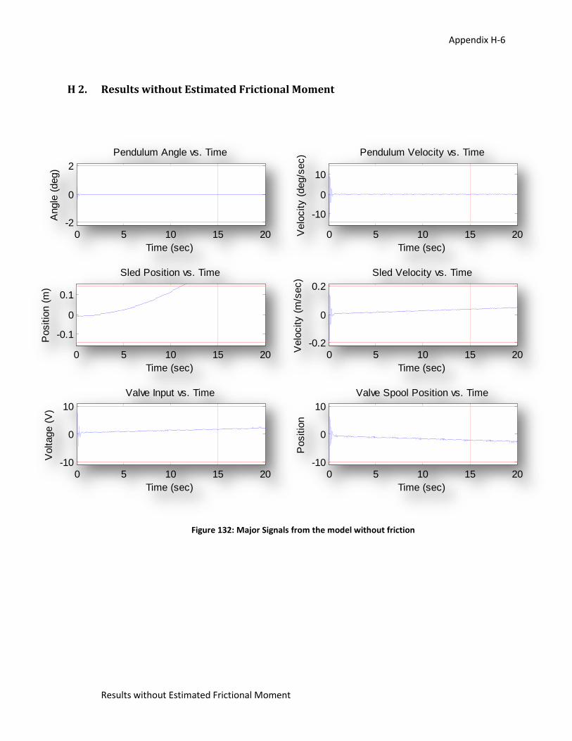
Appendix H-6
Results without Estimated Frictional Moment
H 2. Results without Estimated Frictional Moment
Figure 132: Major Signals from the model without friction
0 5 10 15 20-2
0
2
Pendulum Angle vs. Time
Time (sec)
Angle
(deg)
0 5 10 15 20
-10
0
10
Pendulum Velocity vs. Time
Time (sec)
Velo
city (
deg/s
ec)
0 5 10 15 20
-0.1
0
0.1
Sled Position vs. Time
Time (sec)
Positio
n (
m)
0 5 10 15 20-0.2
0
0.2
Sled Velocity vs. Time
Time (sec)
Velo
city (
m/s
ec)
0 5 10 15 20-10
0
10
Valve Input vs. Time
Time (sec)
Voltage (
V)
0 5 10 15 20-10
0
10
Valve Spool Position vs. Time
Time (sec)
Positio
n
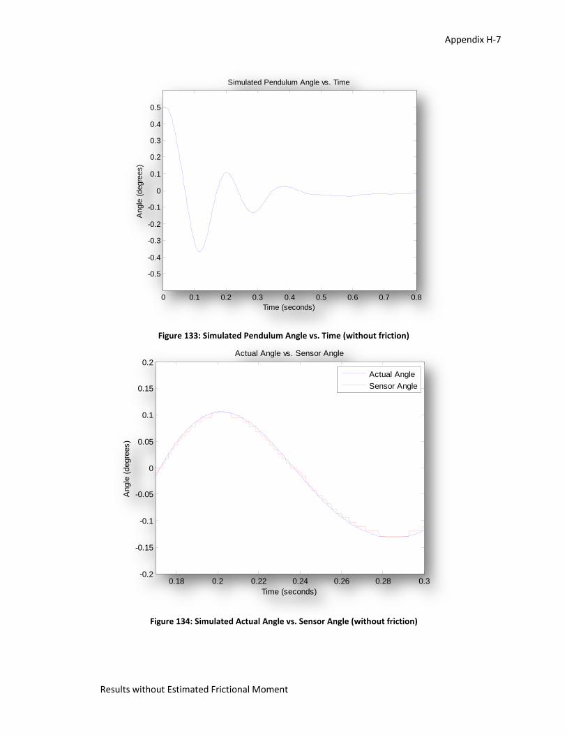
Appendix H-7
Results without Estimated Frictional Moment
Figure 133: Simulated Pendulum Angle vs. Time (without friction)
Figure 134: Simulated Actual Angle vs. Sensor Angle (without friction)
0 0.1 0.2 0.3 0.4 0.5 0.6 0.7 0.8
-0.5
-0.4
-0.3
-0.2
-0.1
0
0.1
0.2
0.3
0.4
0.5
Simulated Pendulum Angle vs. Time
Time (seconds)
Angle
(degre
es)
0.18 0.2 0.22 0.24 0.26 0.28 0.3-0.2
-0.15
-0.1
-0.05
0
0.05
0.1
0.15
0.2Actual Angle vs. Sensor Angle
Time (seconds)
Angle
(degre
es)
Actual Angle
Sensor Angle
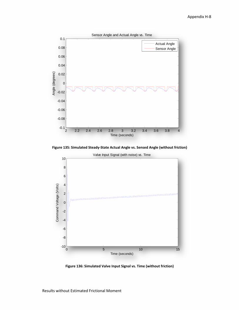
Appendix H-8
Results without Estimated Frictional Moment
Figure 135: Simulated Steady-State Actual Angle vs. Sensed Angle (without friction)
Figure 136: Simulated Valve Input Signal vs. Time (without friction)
2 2.2 2.4 2.6 2.8 3 3.2 3.4 3.6 3.8 4-0.1
-0.08
-0.06
-0.04
-0.02
0
0.02
0.04
0.06
0.08
0.1Sensor Angle and Actual Angle vs. Time
Time (seconds)
Angle
(degre
es)
Actual Angle
Sensor Angle
0 5 10 15-10
-8
-6
-4
-2
0
2
4
6
8
10Valve Input Signal (with noise) vs. Time
Time (seconds)
Com
mand V
oltage (
Volts)
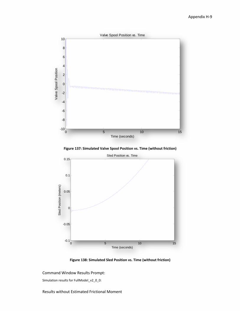
Appendix H-9
Results without Estimated Frictional Moment
Figure 137: Simulated Valve Spool Position vs. Time (without friction)
Figure 138: Simulated Sled Position vs. Time (without friction)
Command Window Results Prompt:
Simulation results for FullModel_v2_0_0:
0 5 10 15-10
-8
-6
-4
-2
0
2
4
6
8
10Valve Spool Position vs. Time
Time (seconds)
Valv
e S
pool P
ositio
n
0 5 10 15-0.1
-0.05
0
0.05
0.1
0.15Sled Position vs. Time
Time (seconds)
Sle
d P
ositio
n (
mete
rs)

Appendix H-10
Results without Estimated Frictional Moment
Pendulum Angle Test: ----PASS---- max test: PASS max limit: 0.0349 rad max value: 0.0087277 rad min test: PASS min limit: -0.0349 rad min value: -0.0064098 rad Pendulum Velocity Test: ----PASS---- max test: PASS max limit: 0.25 rad/s max value: 0.15732 rad/s min test: PASS min limit: -0.25 rad/s min value: -0.21341 rad/s Sled Position Test: ----FAIL---- max test: FAIL max limit: 0.1448 m max value: 0.26684 m min test: PASS min limit: -0.1448 m min value: -0.013619 m Sled Velocity Test: ----PASS---- max test: PASS max limit: 0.2 m/s max value: 0.1377 m/s min test: PASS min limit: -0.2 m/s min value: -0.1913 m/s Valve Input Test: ----FAIL---- max test: PASS max limit: 10 V max value: 7.6719 V min test: FAIL min limit: -10 V min value: -10 V Spool Position Test: ----FAIL---- max test: FAIL max limit: 10 unknown max value: 10 unknown min test: PASS min limit: -10 unknown min value: -9.4382 unknown --------------------------------------------------------------------------- Overall Test: ----FAIL----
Note that the command prompt lists the result as failure. However, in this case, the only signal
of concern was the sled position. The valve input and valve spool positions saturated at their limits at
the beginning of simulation, within a tenth of a second. For times after this point the signals were not
saturated. However, the sled position passed 15 centimeters distance from the center of the hydraulic
cylinder stroke at approximately 11 seconds. Since the time target was 15 seconds, this would not
necessarily be considered a complete success. However, this change in the simulation results from the
results with friction at the joint shows how sensitive the system is to slight changes in modeling. The

Appendix H-11
Results without Estimated Frictional Moment
time the sled was in range can significantly change due to changes in friction, angle bias offset, and
other small effects that may change while the system is in operation. This unpredictable behavior of the
sled position and, consequently, valve input and output signals were also observed in the physical
system.
Appendix I-1
Appendix I: Approach
I 1. Student Personnel
Andrew Hovingh
Oral Communication
o IME102 Research Paper Presentation
Written Communication
o IME102 Research Paper
o Lab Reports for Various ME, ECE, PHYS, and CHEM Courses
o ME365 Reverse Rowing Mechanism Design Project Report
Spatial Communication
o Pro-Engineer
o CadKey 99
Prior Project Experience
o ME365 Reverse Rowing Mechanism Design Project
People Skills
o A Number of Customer Service Experience at Multiple Companies
Research Skills
o IME102 Research Paper
o Researched Parts for Home Built PC
Computer Programming
o Visual Basic 6 Experience
Working Knowledge of Specific Analytical Tools
o MatLAB
o MiniTab
Control and Data Software
o LabVIEW
o MatLAB
Dynamic/Mechanism Analysis Software
o Working Model
FEA Software (Thermal, Flow, Stress, Analysis)
Appendix I-2
Related Work, Internship, Co-op, Experience that might benefit
o Customer Service Experience at Standard Lumber and Target
Experimental/Testing Knowledge
o ME362 Engineering Experimentation
Instrumentation and Transducer Knowledge
o ME335 Engineering Instrumentation
Operating Knowledge of Specific Machines/Test Equipment
Proto-type Build Experience
o Built Proto-type for ME365 Reverse Rowing Mechanism Design Project
Other Beneficial Project Related Skills
Matt Roon
Oral Communication
o Top Negative Speaker in High School Debate
o End of Summer Internship Presentation to over 150 people
Written Communication
o IME102 Research Paper
o End of Summer Internship Report
o ME 365 Speed Reducer Design Report
Spatial Communication
o Pro-Engineer
o AutoCAD 2007
Prior Project Experience
o Pioneered a Dexterous Systematic New Approach for Tracking, Ordering, Replacing, and
Referencing Spare Parts During the Summer Internship
o Design of a Speed Reducer Winch Drum Assembly in ME 365
o Various Metalwork Fabrication Utilizing General Shop Proficiencies
People Skills
o Excelled in Customer Service in Previous Jobs
o Established and Maintained Excellent Customer Relations with Tier-1 Corporations,
Satellite Organizations, and Direct Consumers During the Summer Internship

Appendix I-3
Research Skills
o IME 102 Research Paper
o Various Automation Electronics Research During Summer Internship
o A Plethora of Automotive Research, Specifically in Mustangs, During the Buildup of My
Mustang
Computer Programming
o Two Years Experience in Visual Basic
Working Knowledge of Specific Analytical Tools
o MatLAB
o MiniTab
Control and Data Software
o MatLAB
o LabVIEW
o TWEECER programming experience (software for controlling engine parameters of the
EEC-IV computer in For Mustangs)
Dynamic/Mechanism Analysis Software
o Working Model
o Excel
FEA Software (Thermal, Flow, Stress, Analysis)
o Algor
o Ansys
Related Work, Internship, Co-op, Experience that might benefit
o Innotec Corporation During the Summer of 2006
Experimental/Testing Knowledge
o Think and Do Ladder Logic Programming During Summer Internship
o Various Mechanical Engineering Labs
o ME 362
Instrumentation and Transducer Knowledge
o ME 335
o Thermocouple Experience in Plastic Injection Molding
Operating Knowledge of Specific Machines/Test Equipment
o Robots and Programming

Appendix I-4
o Presses and Progressive Dies
o Plastic Injection Molding Machines
o General Metalwork Shop Proficiencies
Proto-type Build Experience
o Various Metalwork Fabrication Projects
Other Beneficial Project Related Skills
o Excellent Team-Oriented Communication Skills
o Multi-Tasking Skills
I 2. Faculty and Industrial Personnel
Name: Dr. James Kamman
Office: G-222
Department: Mechanical and Aeronautical Engineering
Office Phone: (269) 276-3427
Fax: (269) 276-3421
E-mail: [email protected]
I 3. Responsibility Descriptions
Matt’s Responsibilities:
Mechanical Hardware o Pendulum Design
Length
Bob Weight
Material
Shape
Fasteners
Connection to Pivot Point
o Hinge Design
Bearing Type
Shape
Fasteners
Shaft Length and Diameter
Appendix I-5
Sensor Couplers
o Fixture Design
Material
Size
Shape
Inverted Pendulum Stops
Fasteners
Future Adaptability
Electrical Hardware
o DAQ card adaptability
o Angle Sensor
Analog/Digital
Angular Position/Angular Rate
Connectors/Wiring
CAD Drawings for Pendulum System
Andy’s Responsibilities:
Types of Simulations and Animations
o Simulation of Various Models (MATLAB/Simulink)
Linear/Non-Linear
With/Without Saturation Effects
Type of Controller
User Controls and Program Logic
o Automated Recording and Organizing of Input Parameters
o Tools for Automatic Report Generation of the Results
o Tools for Loading and Creating Calibration Sets for Systems That Meet Performance
Targets
o Function of Switching Between Control Algorithms in MATLAB/Simulink and LabVIEW
o Procedures and Tools for Allowing the System to Calibrate Itself for Changes in the
Physical System
LabVIEW Configuration
Appendix I-6
Shared Responsibilities:
LabVIEW Configuration
CAD Drawings for Pendulum System
I 4. Analytical and Experimental Methods
For the analysis of the project, the main software packages used were MATLAB & Simulink.
MATLAB was used to develop tools, graphical user interfaces, calibration files, and supporting functions
to aid in generating time-response simulations of the motion of the physical system. MATLAB performed
functions such as loading calibration parameters, providing Root-Locus plotting tools for control system
design, plotting results, and generating reports on the success of a simulation based on the calibration
inputs to the model. Simulink was used to create closed loop block diagrams of the dynamics of the
system. Ultimately, the design decisions for sizing individual components were based on hand-written
analytical equations and conclusions, the root-locus diagrams, and the simulation results of the system.
For the experimental component of the design process, a number of experiments were
completed to identify characteristics of components and, finally, tests were performed to determine the
success of the system design. System identification was performed using MATLAB’s system identification
software. The hydraulic cylinder mathematical model coefficients were determined by exciting the
system with some flow rates from a hydraulic pump and valve and recording the motion response of the
cylinder. Once these coefficients were found and the analysis and analytical design was completed, the
system was constructed and LabVIEW, a computer software package, was used to gather sensor input
from the system, execute the desired control algorithm, and output signal commands to the system.
These experiments were done in the motion and control laboratory F-210 at the ParkView Engineering
Campus at Western Michigan University.
Analytical Methods:
Simulation of Physical Motion and Performance: MATLAB & Simulink
Controller Design: MATLAB & Simulink
Experimental Methods:
System Identification: MATLAB & Simulink
Data Acquisition and Control Implementation: LabVIEW
I 5. Expected Deliverables
Reports

Appendix I-7
Weekly meetings and progress reports
Final project report
Final project presentation
Physical System
Engineering and fabrication of inverted pendulum assembly
Proper hydraulic cylinder assembly selection
Proper controller selection
Data
Complete open/closed loop system simulation
LabVIEW programming
DAQ card configuration

Appendix J-1
Appendix J: Resumes
(Next 2 pages)

Appendix K-1
Appendix K: ABET Assessments
Assessment of Program Outcome #5
ME4800
The MAE faculty members have identified “An ability to design a system, component, or
process to meet desired needs within realistic constraints such as economic, environmental, social,
political, ethical, health and safety, manufacturability, and sustainability” as one of the program
outcomes for both mechanical and aeronautical engineering programs. As part of your design project,
we ask you to answer the following questions. You are required to submit the completed form with
your final report in ME 4800. In your final report, please include page references in response to each
question below.
Evaluation of program outcome “An ability to design a system, component, or process to meet
desired needs within realistic constraints such as economic, environmental, social, political, ethical,
health and safety, manufacturability, and sustainability”
1. This project involved the design of a: system / component / process
Description:
_________See section 6. Design
2. The need:
_________See section 1.3: Need
3. The constraints: (Explain and justify any constraint that was relevant to the project. At least 3
constraints must be addressed)
Economic:
_____All physical components’ cost had to be justified within a given budget. The design of the
physical system was adjusted and contorted accordingly.
Environmental :
______________________________________________________________________________
______________________________________________________________________________

Appendix K-2
Social:
______________________________________________________________________________
______________________________________________________________________________
Political:
______________________________________________________________________________
______________________________________________________________________________
Ethical:
______________________________________________________________________________
______________________________________________________________________________
Health& Safety:
______________________________________________________________________________
______________________________________________________________________________
Manufacturability:
_____We were constrained to the physical size of the sled for the overall size of the removable
pendulum system.
Sustainability:
___Reliability and robustness were all considered in the design of the physical system as well as
the software configuration. We were also constrained to educational software such as LabVIEW to
further benefit and aid future students.
Others:
______________________________________________________________________________
______________________________________________________________________________
4. Is there a potential for a new patent in your design? Explain and compare with related
patents.
______________________________________________________________________________
______________________________________________________________________________

Appendix K-3
Assessment of Program Outcome #9
ME 4800
The MAE faculty members have identified “A knowledge of contemporary issues”
as one of the program outcomes for both mechanical and aeronautical engineering programs.
Contemporary issues are any issues that you hear on the news related to new and old products and
their safety, new innovations, technologies, standards and regulations in general. As you develop your
proposal for your senior design project, we ask you to start answering the following questions. These
questions would guide you in the development of ideas you need to include in your proposal and final
project reports. You are required to submit the completed form with your final proposal in ME 4790 and
again with your final report in ME 4800. In your proposal and report, please include page references in
response to each question below.
Evaluation of program outcome “A knowledge of contemporary issues”
1. Why is this project needed now?
This project is for further student knowledge in the area of motion and controls at Western
Michigan University.
2. Describe any new technologies and recent innovations utilized to complete this project.
N/A
3. If this project is done for a company—how will it expand their potential markets?
---how will it improve satisfaction of the company’s existing customers?
N/A
---identify the competitors for this kind of a product, compare the proposed design
with the company’s competitors’ products.
N/A
4. How did you address any safety and/or legal issues pertaining to this project (e.g., OSHA, EPA, Human Factors, etc.).

Appendix K-4
Safety parameters will be utilized in the LabVIEW programming to reduce human error.
5. Are there any new standards or regulations on the horizon that could impact the development of this project? N/A
Is there a potential for a new patent in your design? Please document related patents.
N/A

Appendix K-5
Assessment of Program Outcome #12
ME 4800
The MAE faculty members have identified “An understanding of the impact of the engineering
solutions in a global, environmental and societal context”
as one of the program outcomes for both mechanical and aeronautical engineering programs.
As you develop your proposal for your senior design project, we ask you to start answering the following
questions. These questions would guide you in the development of ideas you need to include in your
proposal and final project reports. You are required to submit the completed form with your final
proposal in ME 4790 and again with your final report in ME 4800. In your proposal and report, please
include page references in response to each question below.
Evaluation of program outcome “An understanding of the impact of the engineering solutions
in a global, environmental and societal context”
1. Is this project useful outside of the United States? Describe why it is or is not-provide details.
Automation and controls have been vastly growing all over the world for precise and accurate
manufacturing processes. This project automates mechanical, hydraulic and electrical systems.
2. Does your project comply with US and/or international standards or regulations? Which standards are applicable?
N/A
3. Is this project restricted in its application to specific markets or communities? To which markets or communities?
This project in its entirety is devoted to the motion and controls laboratory in the Department of
Aeronautical and Mechanical Engineering at Western Michigan University.
4. If the answer to any of the following is positive, explain how and, where relevant, what were
your actions to address the issues?

Appendix K-6
Design is focused on serving human needs. Design also can either negatively or positively
influence quality of life. Address the impact of your project on the following areas.
Air quality?
N/A___________________________________________________________________________
_________________________________________________________________
Water quality?
N/A___________________________________________________________________________
_________________________________________________________________
Food?
N/A___________________________________________________________________________
_________________________________________________________________
Noise level?
N/A___________________________________________________________________________
_________________________________________________________________
Does this project impact:
Human health?
N/A___________________________________________________________________________
_________________________________________________________________
Wildlife?
N/A___________________________________________________________________________
_________________________________________________________________
Vegetation?
N/A___________________________________________________________________________
_________________________________________________________________
Does this project improve:
Human interaction?
N/A___________________________________________________________________________
_________________________________________________________________

Appendix K-7
Well being?
N/A___________________________________________________________________________
_________________________________________________________________
Safety?
N/A___________________________________________________________________________
_________________________________________________________________
Others?
N/A___________________________________________________________________________
_________________________________________________________________

Appendix K-8
Assessment of Program Outcome #13
ME 4800 The MAE faculty have identified “A recognition of the need for, and ability to engage in life-
long learning” as one of the program outcomes for both mechanical and aeronautical
engineering programs. As you develop your proposal for your senior design project, we ask you
to start answering the following questions. These questions will guide you in the development of
ideas you need to include in your proposal and final project reports, as well as help you identify
areas in which you need improved proficiency. You are required to submit the completed form
with your final proposal in ME 4790 and again with your final report in ME 4800 (addressing
slightly different points of view). In your proposal and final project report, please include page
references in response to each question below. This item will be included in the Team Assets
section of the proposal. The format for the response to the questions in the report is of your own
choosing but must address the below listed questions. Questions 2, 3 and 4 will also be directly
addressed in the final Appendix of the report in the format shown below.
Your responses will be used in the Evaluation of program outcome “A recognition of the need
for, and ability to engage in life-long learning”
A well organized team brings necessary backgrounds and talents together that are needed to
successfully execute the design process. Each team member plays an important role on the
design team. Individual members must be prepared to gain any additional skills necessary, and
improve existing skills during project execution.
ME 4800
Mechanical and Aeronautical Engineering Design Project
For each team member:
1. List the skills you needed to execute your responsibilities on the project as outlined in ME
4790.
Matt brings previous automation and controls experience along with vast machining
proficiencies. Andrew brings excellent control simulation and LabVIEW programming
experience.
2. Delineate List how you gained the requisite skill, or enhanced your existing skill, to the
benefit of your design team and the project.
Matt: General fabrication skills will be necessary for the building of the pendulum assembly.
Automation and controls knowledge will be needed for the programming and sensor/controller
integration.
Andrew: LabVIEW programming skills are necessary for the programming skills as well as
knowledge of control systems for the required transfer functions that describe the system.


![Inverted Pendulum [Final]](https://img.pdfslide.net/doc/110x75/58904db31a28abcb668bcda8/inverted-pendulum-final.jpg)