Design and development of Intelligent Mobile Robots (IMRs ...pafkiet.edu.pk/main/wp-content/uploads/2016/09/Second-Deliverable... · Design and development of Intelligent Mobile Robots

Design and development of Intelligent Mobile

Robots (IMRs) for disaster mitigation and

firefighting

Second Deliverable

Report submitted on 6th October 2016

PI: Dr. Muhammad Bilal Kadri

Co-PI: Dr. Tariq Mairaj Rasool Khan

2 | P a g e

Table of Contents

Chapter 1. Introduction ............................................................................................................... 4

Chapter 2. Mechanical Structure of the IMR ............................................................................. 5

2.1 Introduction ...................................................................................................................... 5

2.2 Initial beta hardware ......................................................................................................... 5

2.3 Specifications of the IMR Robot ...................................................................................... 5

2.3.1 Capabilities of IMR Robots ...................................................................................... 5

2.4 IMR Robot 3D Model ...................................................................................................... 6

2.5 Grasping Arm for Hose .................................................................................................... 6

Chapter 3. Electronic Circuitry of the IMR ................................................................................ 7

3.1 IMR Circuit Layout .......................................................................................................... 7

3.2 Sensor placement on the IMR .......................................................................................... 7

3.2.1 UT Sensors ................................................................................................................ 8

3.2.2 Temperature Sensors (RTD-PT100) ....................................................................... 11

3.2.3 Thermal Camera...................................................................................................... 14

3.2.4 Stereo Camera ......................................................................................................... 16

3.2.5 Disparity Map ......................................................................................................... 17

3.2.1 Global Positioning System (GPS) ........................................................................... 18

3.2.2 MAP Generation ..................................................................................................... 20

Chapter 4. Design of Robotic Platform (MUSAFIR) ............................................................... 22

4.1 Motivation ...................................................................................................................... 22

4.2 Desired MUSAFIR Specifications ................................................................................. 22

4.3 3D Design of Musafir ..................................................................................................... 23

4.4 Final LASER Cut Design ............................................................................................... 24

4.5 Motor Selection and Wheels .......................................................................................... 25

4.6 Musafir Electronics ........................................................................................................ 25

4.6.1 Power Circuitry ....................................................................................................... 26

4.6.2 Motor Drivers.......................................................................................................... 26

4.6.3 Motor Controller Board .......................................................................................... 27

3 | P a g e

4.6.4 Sensor Controller .................................................................................................... 28

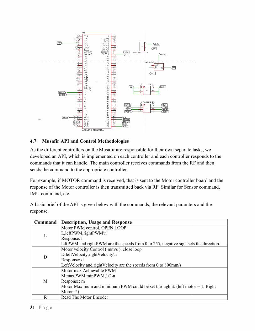
4.6.5 Main Controller Board ............................................................................................ 30

4.6.6 RF Controller Board (PC Side) ............................................................................... 30

4.7 Musafir API and Control Methodologies ....................................................................... 31

4.8 Musafir Actual Robot Images ........................................................................................ 32

Chapter 5. Testing Environment for MUSAFIR ...................................................................... 33

5.1 Test Environment Setup ................................................................................................. 33

5.2 Mubassir – Sub-Components ......................................................................................... 33

5.2.1 Camera .................................................................................................................... 34

5.2.2 Computer System .................................................................................................... 35

5.2.3 Tags on Robots ....................................................................................................... 35

5.3 Mubassir Implementation ............................................................................................... 36

5.4 Software environment .................................................................................................... 36

5.5 Accessing Mubassir Data ............................................................................................... 37

Chapter 6. Control Algorithm Development ............................................................................ 38

6.1 Introduction .................................................................................................................... 38

6.2 Simulation Results.......................................................................................................... 38

6.3 Simulink Model Approach: ............................................................................................ 40

6.4 Mobile Robots Swarm (Trajectory for Virtual Only) .................................................... 41

Chapter 7. Robot Localization by sensor fusion of GPS, Odometer and INS .......................... 49

Chapter 8. Annexure A ............................................................................................................. 55

Chapter 9. Annexure B ............................................................................................................. 57

Chapter 10. Annexure C ...................................................................................................... 64

4 | P a g e

Chapter 1. Introduction

This report is the second deliverable for the National ICTR&D funded research project titled

“Design and development of Intelligent Mobile Robots (IMRs) for disaster mitigation and

firefighting”.

5 | P a g e

Chapter 2. Mechanical Structure of the IMR

2.1 Introduction

Mechanical Structure of IMR is being developed alongside the electronics and the power

circuitry. As the mechanical structure design relies on all of the former developments. i.e. sensor

placements, number of sensors, number of motors, tyre type, size dimensions, inner space

requirements, power supply – all these parameters need to be finalized before the hardware

design can be finalized. Hence the hardware design process is in a very variable state.

Additionally, the IMR hardware needs to be relaible enough to withstand high temperatures and

some impact on the body. The body also needs to be somewhat waterproof to safeguard the inner

batteries, motors and other circuitry, for these reasons, the IMR hardware design is broken into

multiple stages, with the first stage being the development of a basic hardware chassis, which

will serve as a testing ground to refine the final design and the actual IMR hardware will be

developed ONLY after the initial beta hardware is tested thoroughly.

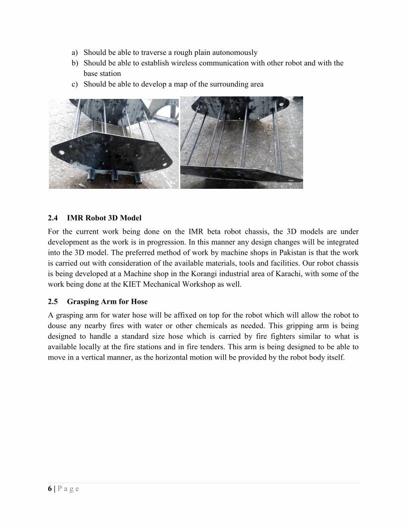
2.2 Initial beta hardware

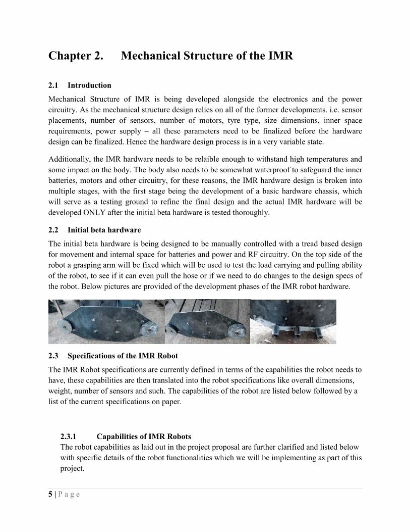
The initial beta hardware is being designed to be manually controlled with a tread based design

for movement and internal space for batteries and power and RF circuitry. On the top side of the

robot a grasping arm will be fixed which will be used to test the load carrying and pulling ability

of the robot, to see if it can even pull the hose or if we need to do changes to the design specs of

the robot. Below pictures are provided of the development phases of the IMR robot hardware.

2.3 Specifications of the IMR Robot

The IMR Robot specifications are currently defined in terms of the capabilities the robot needs to

have, these capabilities are then translated into the robot specifications like overall dimensions,

weight, number of sensors and such. The capabilities of the robot are listed below followed by a

list of the current specifications on paper.

2.3.1 Capabilities of IMR Robots

The robot capabilities as laid out in the project proposal are further clarified and listed below

with specific details of the robot functionalities which we will be implementing as part of this

project.

6 | P a g e

a) Should be able to traverse a rough plain autonomously

b) Should be able to establish wireless communication with other robot and with the

base station

c) Should be able to develop a map of the surrounding area

2.4 IMR Robot 3D Model

For the current work being done on the IMR beta robot chassis, the 3D models are under

development as the work is in progression. In this manner any design changes will be integrated

into the 3D model. The preferred method of work by machine shops in Pakistan is that the work

is carried out with consideration of the available materials, tools and facilities. Our robot chassis

is being developed at a Machine shop in the Korangi industrial area of Karachi, with some of the

work being done at the KIET Mechanical Workshop as well.

2.5 Grasping Arm for Hose

A grasping arm for water hose will be affixed on top for the robot which will allow the robot to

douse any nearby fires with water or other chemicals as needed. This gripping arm is being

designed to handle a standard size hose which is carried by fire fighters similar to what is

available locally at the fire stations and in fire tenders. This arm is being designed to be able to

move in a vertical manner, as the horizontal motion will be provided by the robot body itself.

7 | P a g e

Chapter 3. Electronic Circuitry of the IMR

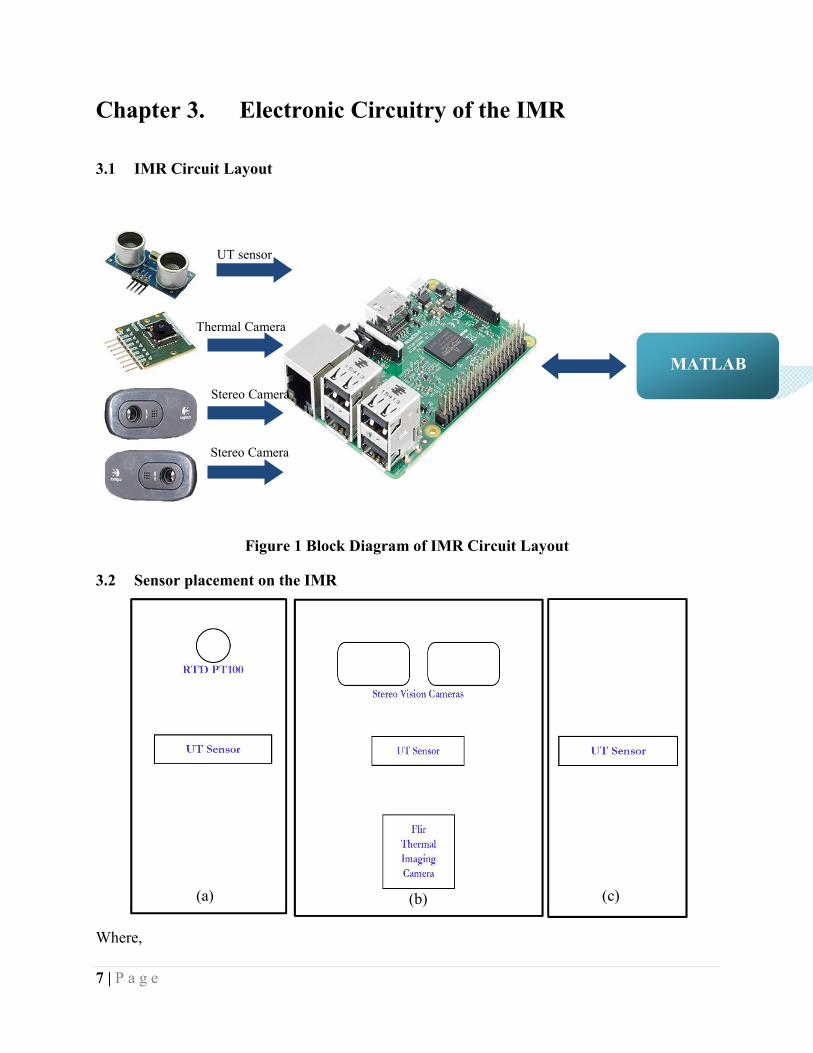
3.1 IMR Circuit Layout

Figure 1 Block Diagram of IMR Circuit Layout

3.2 Sensor placement on the IMR

Where,

MATLAB

UT sensor

Thermal Camera

Stereo Camera

Stereo Camera

(a) (b) (c)

8 | P a g e

(a) => Right Side view of sensors on IMR

(b) => Front Side view of sensors on IMR

(c) => Left Side view of sensors on IMR

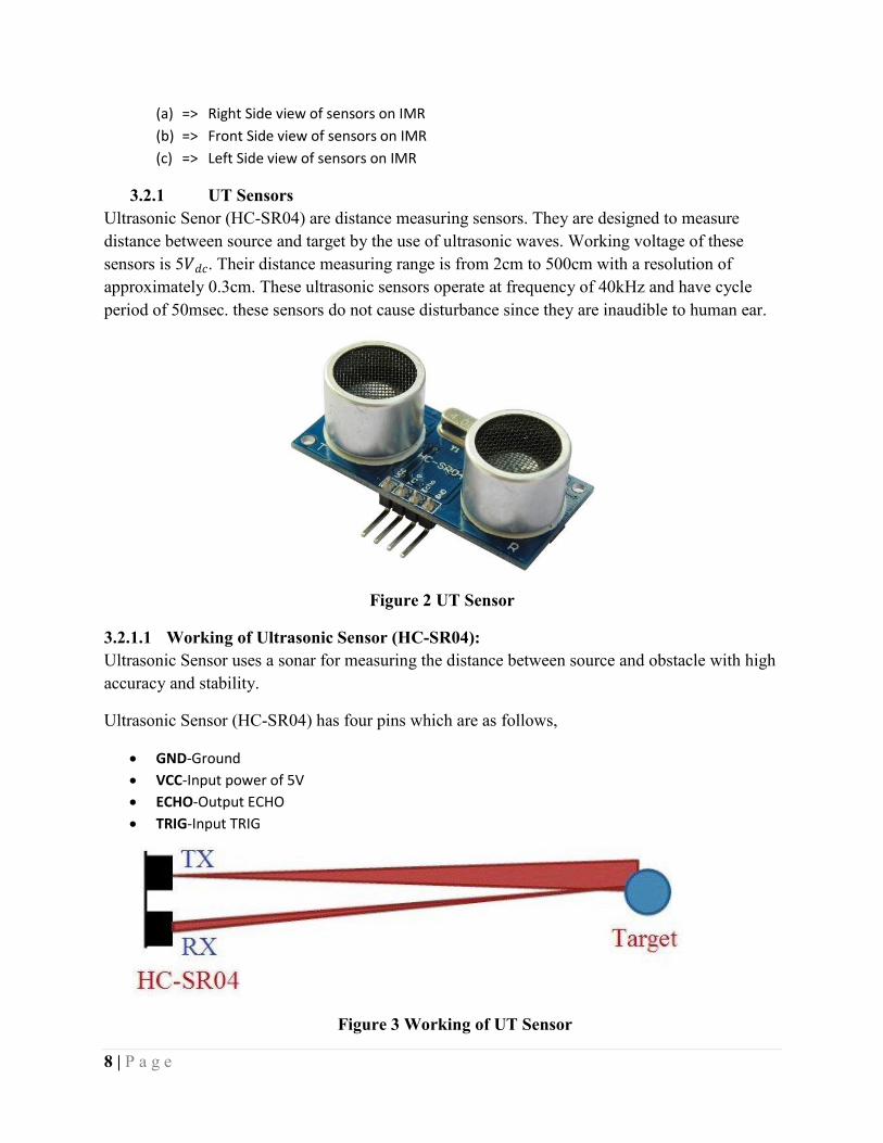
3.2.1 UT Sensors

Ultrasonic Senor (HC-SR04) are distance measuring sensors. They are designed to measure

distance between source and target by the use of ultrasonic waves. Working voltage of these

sensors is 5��. Their distance measuring range is from 2cm to 500cm with a resolution of

approximately 0.3cm. These ultrasonic sensors operate at frequency of 40kHz and have cycle

period of 50msec. these sensors do not cause disturbance since they are inaudible to human ear.

Figure 2 UT Sensor

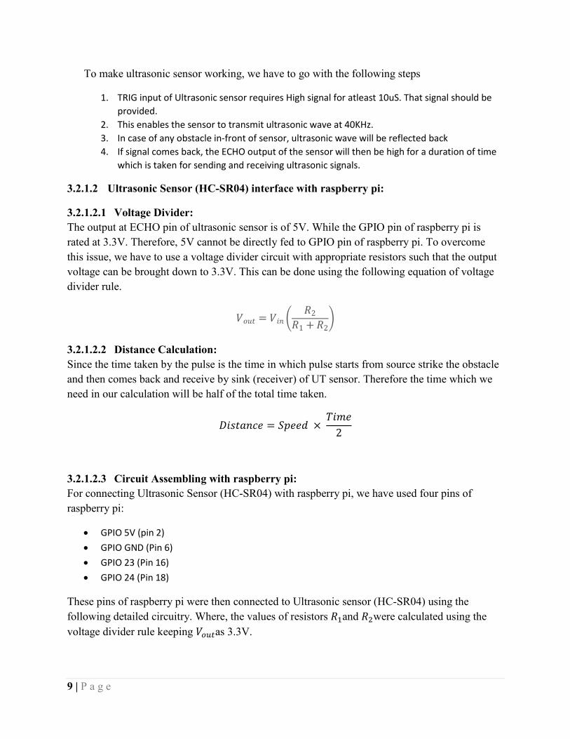
3.2.1.1 Working of Ultrasonic Sensor (HC-SR04):

Ultrasonic Sensor uses a sonar for measuring the distance between source and obstacle with high

accuracy and stability.

Ultrasonic Sensor (HC-SR04) has four pins which are as follows,

GND-Ground

VCC-Input power of 5V

ECHO-Output ECHO

TRIG-Input TRIG

Figure 3 Working of UT Sensor

9 | P a g e

To make ultrasonic sensor working, we have to go with the following steps

1. TRIG input of Ultrasonic sensor requires High signal for atleast 10uS. That signal should be

provided.

2. This enables the sensor to transmit ultrasonic wave at 40KHz.

3. In case of any obstacle in-front of sensor, ultrasonic wave will be reflected back

4. If signal comes back, the ECHO output of the sensor will then be high for a duration of time

which is taken for sending and receiving ultrasonic signals.

3.2.1.2 Ultrasonic Sensor (HC-SR04) interface with raspberry pi:

3.2.1.2.1 Voltage Divider:

The output at ECHO pin of ultrasonic sensor is of 5V. While the GPIO pin of raspberry pi is

rated at 3.3V. Therefore, 5V cannot be directly fed to GPIO pin of raspberry pi. To overcome

this issue, we have to use a voltage divider circuit with appropriate resistors such that the output

voltage can be brought down to 3.3V. This can be done using the following equation of voltage

divider rule.

�� = �� 2

�1 + �2�

3.2.1.2.2 Distance Calculation:

Since the time taken by the pulse is the time in which pulse starts from source strike the obstacle

and then comes back and receive by sink (receiver) of UT sensor. Therefore the time which we

need in our calculation will be half of the total time taken.

�� = �� × ��

2

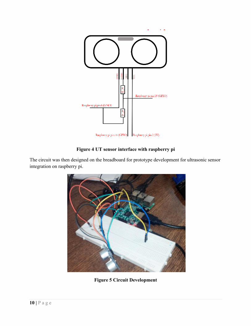
3.2.1.2.3 Circuit Assembling with raspberry pi:

For connecting Ultrasonic Sensor (HC-SR04) with raspberry pi, we have used four pins of

raspberry pi:

GPIO 5V (pin 2)

GPIO GND (Pin 6)

GPIO 23 (Pin 16)

GPIO 24 (Pin 18)

These pins of raspberry pi were then connected to Ultrasonic sensor (HC-SR04) using the

following detailed circuitry. Where, the values of resistors ��and ��were calculated using the

voltage divider rule keeping ��as 3.3V.

10 | P a g e

Figure 4 UT sensor interface with raspberry pi

The circuit was then designed on the breadboard for prototype development for ultrasonic sensor

integration on raspberry pi.

Figure 5 Circuit Development

11 | P a g e

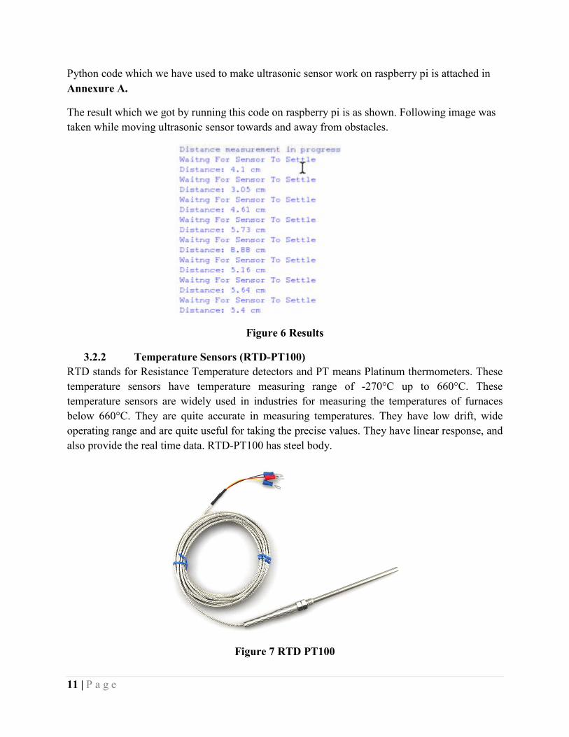
Python code which we have used to make ultrasonic sensor work on raspberry pi is attached in

Annexure A.

The result which we got by running this code on raspberry pi is as shown. Following image was

taken while moving ultrasonic sensor towards and away from obstacles.

3.2.2 Temperature Sensors

RTD stands for Resistance Temperature detectors and PT means Platinum thermometers.

temperature sensors have temperature measuring range of

temperature sensors are widely used in industries for measuring the temperatures

below 660°C. They are quite accurate in measuring temperatures. They have low drift, wide

operating range and are quite useful for taking the precise values

also provide the real time data. RTD



sensor towards and away from obstacles.

Figure 6 Results

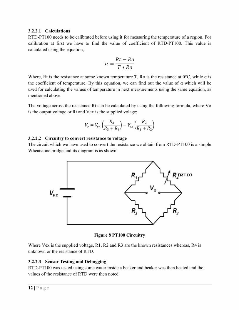
Temperature Sensors (RTD-PT100)

RTD stands for Resistance Temperature detectors and PT means Platinum thermometers.

have temperature measuring range of -270°C up to 660°C.

temperature sensors are widely used in industries for measuring the temperatures


operating range and are quite useful for taking the precise values. They have linear response, and

also provide the real time data. RTD-PT100 has steel body.

Figure 7 RTD PT100



RTD stands for Resistance Temperature detectors and PT means Platinum thermometers. These

270°C up to 660°C. These

temperature sensors are widely used in industries for measuring the temperatures of furnaces


. They have linear response, and

12 | P a g e

3.2.2.1 Calculations

RTD-PT100 needs to be calibrate

calibration at first we have to find the value of coefficient of RTD

calculated using the equation,

Where, Rt is the resistance at some known temperatu

the coefficient of temperature. By this equation, we can find out the value of α which will be

used for calculating the values of temperature in next measurements using the same equation, as

mentioned above.

The voltage across the resistance Rt can be calculated by using the following formula, where Vo

is the output voltage or Rt and Vex is the supplied volage;

��

3.2.2.2 Circuitry to convert resistance to voltage

The circuit which we have used to convert the resistance we obtain from RTD

Wheatstone bridge and its diagram is as shown:

Where Vex is the supplied voltage, R1, R2 and R3 are the known resistances whereas, R4 is

unknown or the resistance of RTD.

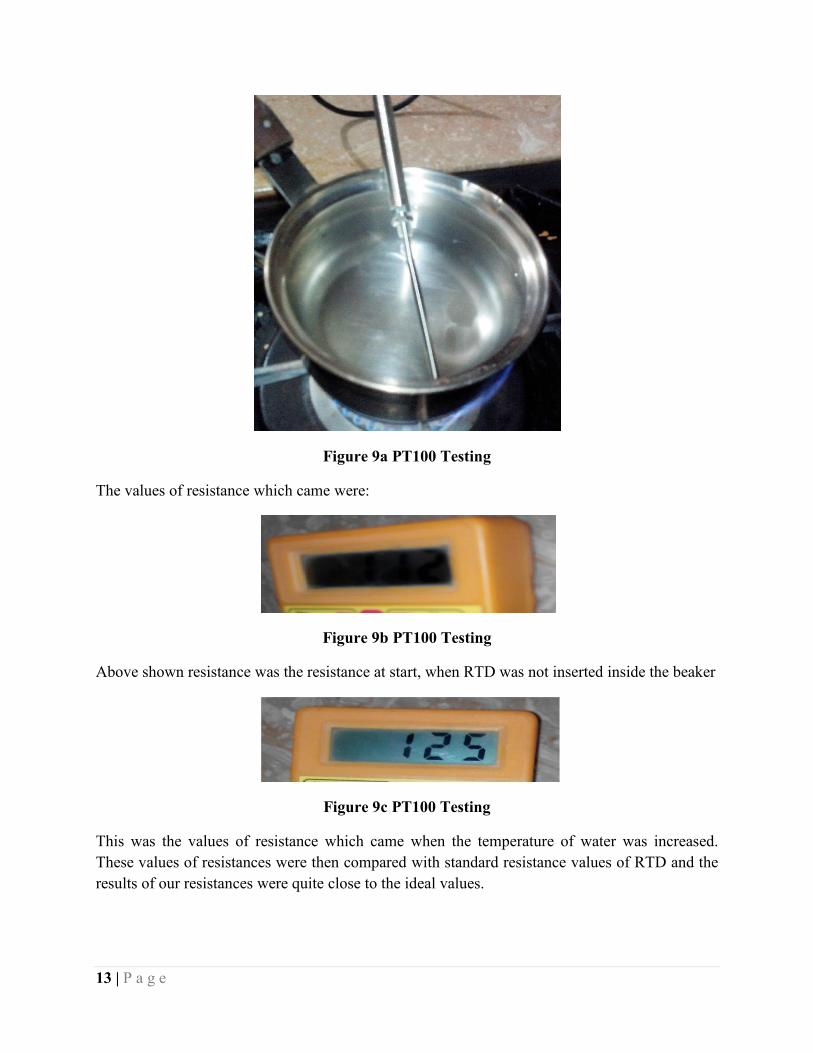
3.2.2.3 Sensor Testing and Debugging

RTD-PT100 was tested using some water inside a beaker and beaker was then heated and the

values of the resistance of RTD were then noted

calibrated before using it for measuring the temperature of a region. For

calibration at first we have to find the value of coefficient of RTD-PT100. This value is

� =�� − ��

� ∗ ��

Where, Rt is the resistance at some known temperature T, Ro is the resistance at 0



e voltage across the resistance Rt can be calculated by using the following formula, where Vo

is the output voltage or Rt and Vex is the supplied volage;

= ��

�� + �� − ��

��

�� + ��

Circuitry to convert resistance to voltage

e have used to convert the resistance we obtain from RTD-PT100 is a simple

Wheatstone bridge and its diagram is as shown:

Figure 8 PT100 Circuitry


sistance of RTD.

Sensor Testing and Debugging

PT100 was tested using some water inside a beaker and beaker was then heated and the

values of the resistance of RTD were then noted

before using it for measuring the temperature of a region. For

PT100. This value is

re T, Ro is the resistance at 0°C, while α is



e voltage across the resistance Rt can be calculated by using the following formula, where Vo

PT100 is a simple


PT100 was tested using some water inside a beaker and beaker was then heated and the

13 | P a g e

The values of resistance which came were:

Above shown resistance was the resistance at start, when RTD was not inserted inside the beaker

This was the values of resistance which came when the temperature of water was increased.

These values of resistances were then compared with standard resistance values of RTD and the

results of our resistances were quite close to the ideal values.

Figure 9a PT100 Testing

The values of resistance which came were:

Figure 9b PT100 Testing


Figure 9c PT100 Testing


stances were then compared with standard resistance values of RTD and the

results of our resistances were quite close to the ideal values.



stances were then compared with standard resistance values of RTD and the

14 | P a g e

3.2.3 Thermal Camera

3.2.3.1 Electromagnetic Spectrum for Flir Thermal Imaging Camera

Electromagnetic radiations are available all

ranging from Gamma radiations on the higher frequency side and radio waves on lower

frequency side. Most of the sensors used for imaging purposes detect radiations only in visible

region of spectrum (wavelength is from 380nm to 700nm), while infrared wave sensors detect

radiations from 900nm to 14,000nm which is known as infrared spectrum. It accounts for most

of the thermal radiations emitted by objects near room temperature.

Figure 10 Spectrum of Thermal I

Microbolometer array is the sensor which is used insed the FLiR Lepton. Microbolometers are made from a material which changes its resistance when they are heated up by infrared radiations. By calculating this resistance, we can determine theis emitting those radiations and create a false color image which encodes that data.

This type of thermal imaging technique is often used for inspection of buildings, to detect insulation leakage, automotive inspection andimage with no visible light, therefore thermal imaging is considered ideal for night vision cameras.

3.2.3.2 Circuit Assembling with Raspberry pi

For connecting raspberry pi with Flir thermal imaging camera we have

connections,

Pin 1 of raspberry pi (Vcc=3.3V) : Vin of Flir thermal imaging camera

Pin 3 of raspberry pi : SDA pin of flir thermal imaging camera

Pin 5 of raspberry pi : SCL pin of flir thermal imaging camera

Pin 6 of raspberry pi (GND)

Pin 19 of raspberry pi : MOSI pin of flir thermal imaging camera

Thermal Camera

Electromagnetic Spectrum for Flir Thermal Imaging Camera

Electromagnetic radiations are available all around us and they are comprised of


requency side. Most of the sensors used for imaging purposes detect radiations only in visible

th is from 380nm to 700nm), while infrared wave sensors detect


of the thermal radiations emitted by objects near room temperature.

Figure 10 Spectrum of Thermal Imaging Camera

Microbolometer array is the sensor which is used insed the FLiR Lepton. Microbolometers are made from a material which changes its resistance when they are heated up by infrared radiations. By calculating this resistance, we can determine the temperature of that object which is emitting those radiations and create a false color image which encodes that data.

This type of thermal imaging technique is often used for inspection of buildings, to detect insulation leakage, automotive inspection and medical diagnosis. it has ability to produce the image with no visible light, therefore thermal imaging is considered ideal for night vision

Circuit Assembling with Raspberry pi

For connecting raspberry pi with Flir thermal imaging camera we have used the following

Pin 1 of raspberry pi (Vcc=3.3V) : Vin of Flir thermal imaging camera

Pin 3 of raspberry pi : SDA pin of flir thermal imaging camera

Pin 5 of raspberry pi : SCL pin of flir thermal imaging camera

Pin 6 of raspberry pi (GND) : GND of flir thermal imaging camera

Pin 19 of raspberry pi : MOSI pin of flir thermal imaging camera

around us and they are comprised of radiations


requency side. Most of the sensors used for imaging purposes detect radiations only in visible

th is from 380nm to 700nm), while infrared wave sensors detect


Microbolometer array is the sensor which is used insed the FLiR Lepton. Microbolometers are made from a material which changes its resistance when they are heated up by infrared

temperature of that object which is emitting those radiations and create a false color image which encodes that data.

This type of thermal imaging technique is often used for inspection of buildings, to detect medical diagnosis. it has ability to produce the

image with no visible light, therefore thermal imaging is considered ideal for night vision

used the following

15 | P a g e

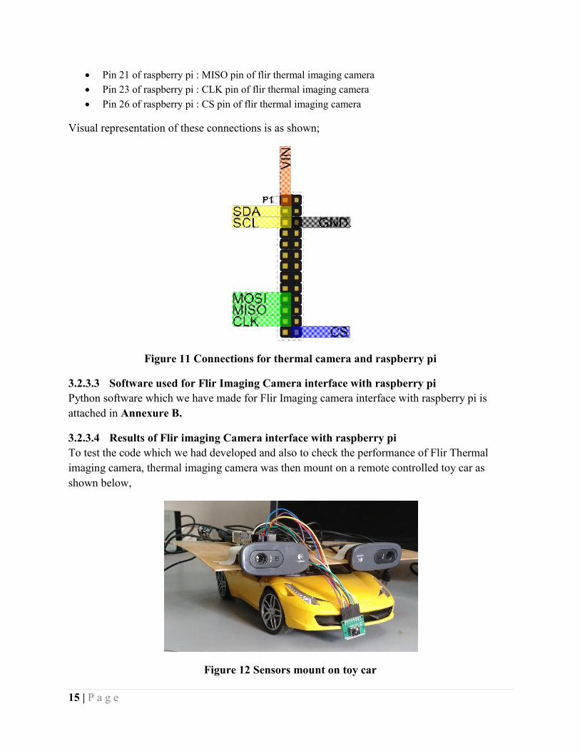
Pin 21 of raspberry pi : MISO pin of flir thermal imaging camera

Pin 23 of raspberry pi : CLK pin of flir thermal imaging camera

Pin 26 of raspberry pi : CS pin of flir thermal imaging camera

Visual representation of these connections is as shown;

Figure 11 Connections for thermal camera and raspberry pi

3.2.3.3 Software used for Flir Imaging Camera interface with raspberry pi

Python software which we have made for Flir Imaging camera interface with raspberry pi is

attached in Annexure B.

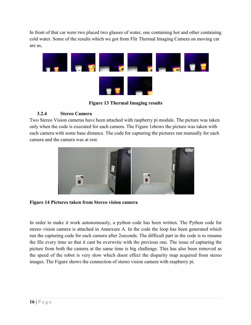
3.2.3.4 Results of Flir imaging Camera interface with raspberry pi

To test the code which we had developed and also to check the performance of Flir T

imaging camera, thermal imaging camera was then mount on a remote controlled toy car as

shown below,

Figure 12 Sensors mount on toy car

Pin 21 of raspberry pi : MISO pin of flir thermal imaging camera

Pin 23 of raspberry pi : CLK pin of flir thermal imaging camera

CS pin of flir thermal imaging camera

Visual representation of these connections is as shown;


Software used for Flir Imaging Camera interface with raspberry pi


Results of Flir imaging Camera interface with raspberry pi

To test the code which we had developed and also to check the performance of Flir T


Figure 12 Sensors mount on toy car


Software used for Flir Imaging Camera interface with raspberry pi


To test the code which we had developed and also to check the performance of Flir Thermal


16 | P a g e

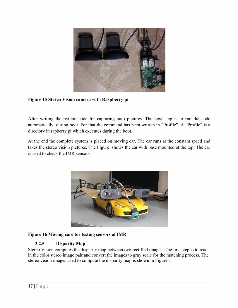
In front of that car were two placed two glasses of water, one containing hot and other containing

cold water. Some of the results which we got from Flir Thermal Imaging Camera on moving car

are as,

Figure 13 Thermal Imaging results

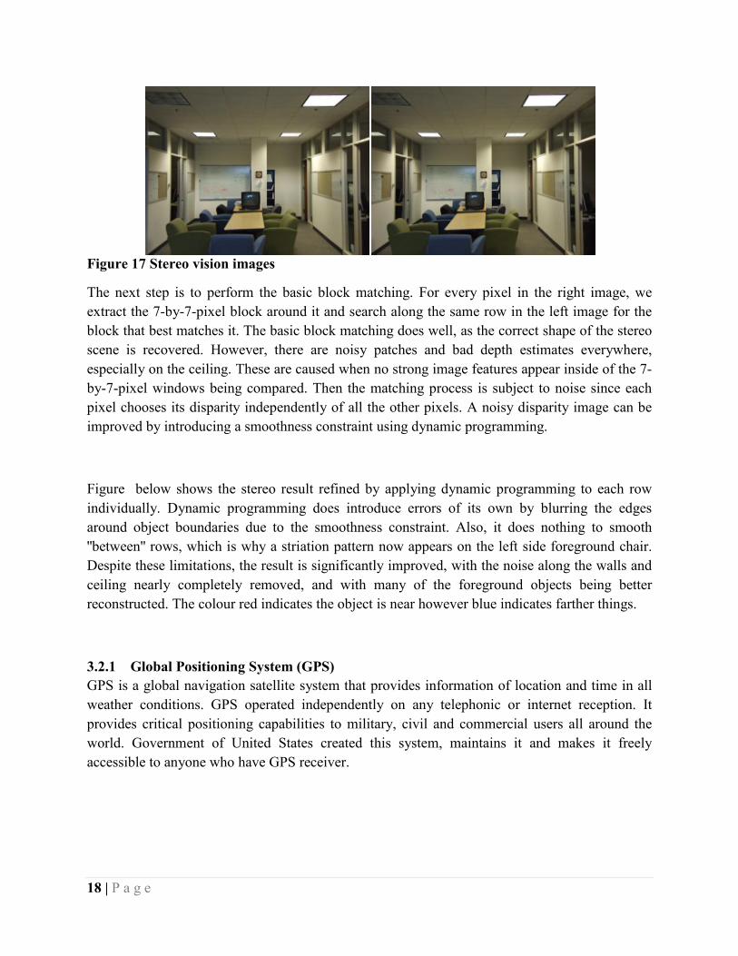
3.2.4 Stereo Camera

Two Stereo Vision cameras have been attached with raspberry pi module. The picture was taken

only when the code is executed for each camera. The Figure 1shows the picture was taken with

each camera with some base distance. The code for capturing the pictures run manually for each

camera and the camera was at rest.

Figure 14 Pictures taken from Stereo vision camera

In order to make it work autonomously, a python code has been written. The Python code for

stereo vision camera is attached in Annexure A. In the code the loop has been generated which

run the capturing code for each camera after 2seconds. The difficult part in the code is to rename

the file every time so that it cant be overwrite with the previous one. The issue of capturing the

picture from both the camera at the same time is big challenge. This has also been removed as

the speed of the robot is very slow which doest effect the disparity map acquired from stereo

images. The Figure shows the connection of stereo vision camera with raspberry pi.

17 | P a g e

Figure 15 Stereo Vision camera with Raspberry pi

After writing the python code for capturing auto pictures. The next step is to run the code

automatically during boot. For that the command has been written in “Profile”. A “Profile” is a

directory in rapberry pi which executes during the boot.

At the end the complete system is placed on moving car. The car runs at the constant speed and

takes the stereo vision pictures. The Figure shows the car with base mounted at the top. The car

is used to check the IMR sensors.

Figure 16 Moving care for testing sensors of IMR

3.2.5 Disparity Map

Stereo Vision computes the disparity map between two rectified images. The first step is to read in the color stereo image pair and convert the images to gray scale for the matching process. The stereo vision images used to compute the disparity map is shown in Figure .

18 | P a g e

Figure 17 Stereo vision images

The next step is to perform the basic block matching. For every pixel in the right image, we

extract the 7-by-7-pixel block around it and search along the same row in the left image for the

block that best matches it. The basic block matching does well, as the correct shape of the stereo

scene is recovered. However, there are noisy patches and bad depth estimates everywhere,

especially on the ceiling. These are caused when no strong image features appear inside of the 7-

by-7-pixel windows being compared. Then the matching process is subject to noise since each

pixel chooses its disparity independently of all the other pixels. A noisy disparity image can be

improved by introducing a smoothness constraint using dynamic programming.

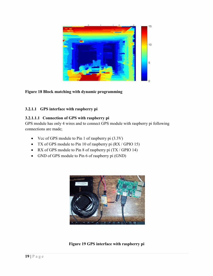
Figure below shows the stereo result refined by applying dynamic programming to each row

individually. Dynamic programming does introduce errors of its own by blurring the edges

around object boundaries due to the smoothness constraint. Also, it does nothing to smooth

''between'' rows, which is why a striation pattern now appears on the left side foreground chair.

Despite these limitations, the result is significantly improved, with the noise along the walls and

ceiling nearly completely removed, and with many of the foreground objects being better

reconstructed. The colour red indicates the object is near however blue indicates farther things.

3.2.1 Global Positioning System (GPS)

GPS is a global navigation satellite system that provides information of location and time in all

weather conditions. GPS operated independently on any telephonic or internet reception. It

provides critical positioning capabilities to military, civil and commercial users all around the

world. Government of United States created this system, maintains it and makes it freely

accessible to anyone who have GPS receiver.

19 | P a g e

Figure 18 Block matching with dynamic programming

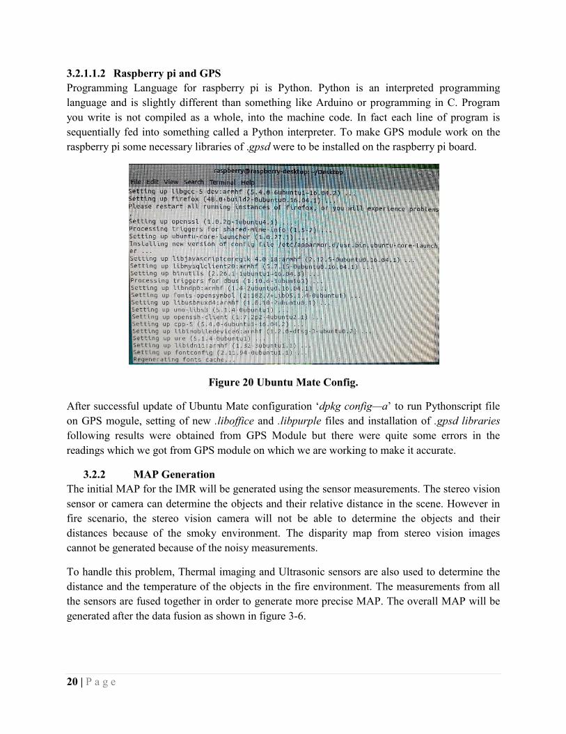
3.2.1.1 GPS interface with raspberry pi

3.2.1.1.1 Connection of GPS with raspberry pi

GPS module has only 4 wires and to connect GPS module with raspberry pi following

connections are made;

Vcc of GPS module to Pin 1 of raspberry pi (3.3V)

TX of GPS module to Pin 10 of raspberry pi (RX / GPIO 15)

RX of GPS module to Pin 8 of raspberry pi (TX / GPIO 14)

GND of GPS module to Pin 6 of raspberry pi (GND)

Figure 19 GPS interface with raspberry pi

20 | P a g e

3.2.1.1.2 Raspberry pi and GPS

Programming Language for raspberry pi is Python. Python is an interpreted programming

language and is slightly different than something like Arduino or programming in C. Program

you write is not compiled as a whole, into the machine code. In fact each line of program is

sequentially fed into something called a Python interpreter. To make GPS module work on the

raspberry pi some necessary libraries of .gpsd were to be installed on the raspberry pi board.

Figure 20 Ubuntu Mate Config.

After successful update of Ubuntu Mate configuration ‘dpkg config—a’ to run Pythonscript file

on GPS mogule, setting of new .liboffice and .libpurple files and installation of .gpsd libraries

following results were obtained from GPS Module but there were quite some errors in the

readings which we got from GPS module on which we are working to make it accurate.

3.2.2 MAP Generation

The initial MAP for the IMR will be generated using the sensor measurements. The stereo vision

sensor or camera can determine the objects and their relative distance in the scene. However in

fire scenario, the stereo vision camera will not be able to determine the objects and their

distances because of the smoky environment. The disparity map from stereo vision images

cannot be generated because of the noisy measurements.

To handle this problem, Thermal imaging and Ultrasonic sensors are also used to determine the

distance and the temperature of the objects in the fire environment. The measurements from all

the sensors are fused together in order to generate more precise MAP. The overall MAP will be

generated after the data fusion as shown in figure 3-6.

21 | P a g e

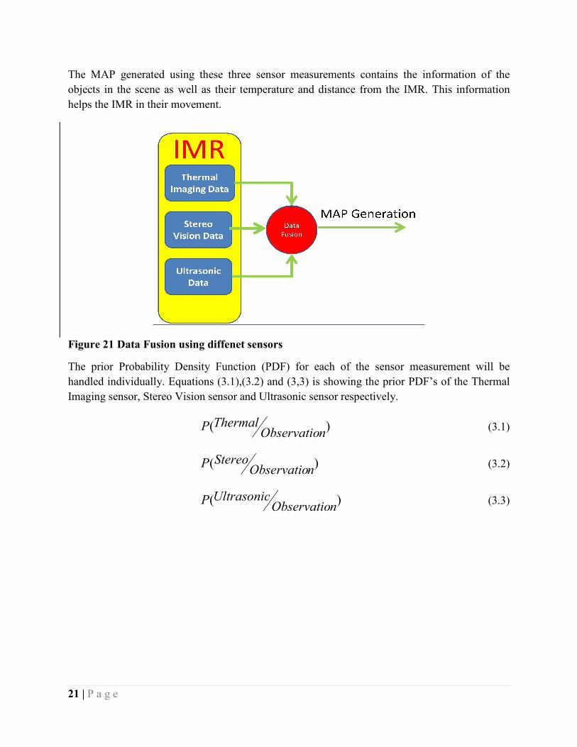
The MAP generated using these three sensor measurements contains the information of the

objects in the scene as well as their temperature and distance from the IMR. This information

helps the IMR in their movement.

Figure 21 Data Fusion using diffenet sensors

The prior Probability Density Function (PDF) for each of the sensor measurement will be

handled individually. Equations (3.1),(3.2) and (3,3) is showing the prior PDF’s of the Thermal

Imaging sensor, Stereo Vision sensor and

(ThermalP

(StereoP

(UltrasonicP



helps the IMR in their movement.

a Fusion using diffenet sensors



Imaging sensor, Stereo Vision sensor and Ultrasonic sensor respectively.

)nObservatio

Thermal

)nObservatio

Stereo

)nObservatio

Ultrasonic





(3.1)

(3.2)

(3.3)

22 | P a g e

Chapter 4. Design of Robotic Platform (MUSAFIR)

4.1 Motivation

MUSAFIR is an Urdu word, which means Traveler. In order to design and build robots for the

IMR project, we need to test several algorithms and work on several different sensing

techniques. In order to be able to reliably and repeatedly test the algorithms, we needed a test

robotic platform. Musafir is the result of that need.

The Musafir design is mainly inspired from some similar academic commercial bots, which are

too expensive Khepera (I, II, III and now IV) and e-Puck Robot, the 2 Commercial Academic

Research Mobile Robotic Platforms are the 2 prime example robotic platforms that we have

studied. We selected to mimic Khepera robots as these robots are also the ones used by other

robotics labs around the world and also included in the online course CONTROL OF MOBILE

ROBOTS - https://www.coursera.org/learn/mobile-robot

For comparison, the cost of Khepera IV is 2650CHF which is about 2695 USD and 282,554 PKR

and cost of e-puck, another similar robot is 950 CHF, which is 966USD and 101,293 PKR. This

is excluding the customs and shipping expenses.

Musafir robot is expected to be built in a fraction of the cost and we are working to make 4 such

robots, so that most of the collaborative control, SLAM and swarm algorithms can be tested,

most configurations require at least 3 to 4 robots.

4.2 Desired MUSAFIR Specifications

In order to design and build a new robotics platform, specifications need to be written and laid

out before starting the work. Musafir robots are expected to have several built-in sensors and

communication methods.

Re-Chargeable Battery

Round/Circular/Symmetric Design

IR/Sonar sensor skirt around the bot

Differential Drive Motors with Encoders

IMU (Gyro + Accelerometer) + Compass Sensor

Wireless Communication

Motor Driver - MOSFET Based

On-board computer/camera for further processing and SLAM – OPTIONAL

With these specifications, the design was broken into 3 main steps, initially a very basic robotic

platform with motors and wireless control and minimum sensors will be implemented, then the

design will be refined and more sensors (sensor skirt) will be added to the bot, finally, in the

23 | P a g e

third stage the robot will be equipped with a computer (Raspberry Pi) and a camera, given time

and budget constraints, this step will be done last and is optional.

4.3 3D Design of Musafir

Musafir robot was first designed in SolidWorks, however

was needed to be done with Acrylic Plastic Sheets, which are cut by laser cut CNC machines, the

design was also re-done in SketchUp and then further refined in CorelDraw for final sending to

the Laser Cut shop.

The designs are provided below which serve as a reference and show how the design evolved

over time.

Figure 4-1: Initial Sketch of Robot base, showing Motors and Ball Caster Wheels

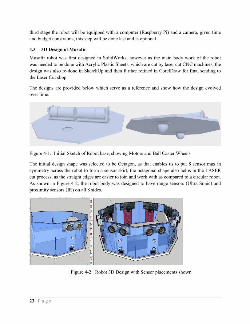
The initial design shape was selected to be Octagon, as that enables us to put 8

symmetry across the robot to form a sensor skirt, the octagonal shape also helps in the LASER

cut process, as the straight edges are easier to join and work with as compared to a circular robot.

As shown in Figure 4-2, the robot body was des

proximity sensors (IR) on all 8 sides.

Figure 4-2: Robot 3D Design with Sensor placements shown


and budget constraints, this step will be done last and is optional.

Musafir robot was first designed in SolidWorks, however as the main body work of the robot


done in SketchUp and then further refined in CorelDraw for final sending to

ns are provided below which serve as a reference and show how the design evolved

1: Initial Sketch of Robot base, showing Motors and Ball Caster Wheels

The initial design shape was selected to be Octagon, as that enables us to put 8



2, the robot body was designed to have range sensors (Ultra Sonic) and

proximity sensors (IR) on all 8 sides.

2: Robot 3D Design with Sensor placements shown


as the main body work of the robot


done in SketchUp and then further refined in CorelDraw for final sending to

ns are provided below which serve as a reference and show how the design evolved

1: Initial Sketch of Robot base, showing Motors and Ball Caster Wheels

The initial design shape was selected to be Octagon, as that enables us to put 8 sensor max in



igned to have range sensors (Ultra Sonic) and

2: Robot 3D Design with Sensor placements shown

24 | P a g e

4.4 Final LASER Cut Design

For first iteration, the Musafir design was minimized to a Minimum working Prototype Stage

(without computer and sensor skirt) and re-designed in Corel Draw for LASER Cut work, the

final design 2D planar top view is shown in Figure 4-3 (not to scale).

Figure 4-3: Profile for LASER Cutting – Size: 256x256mm – Thickness 5mm Acrylic

25 | P a g e

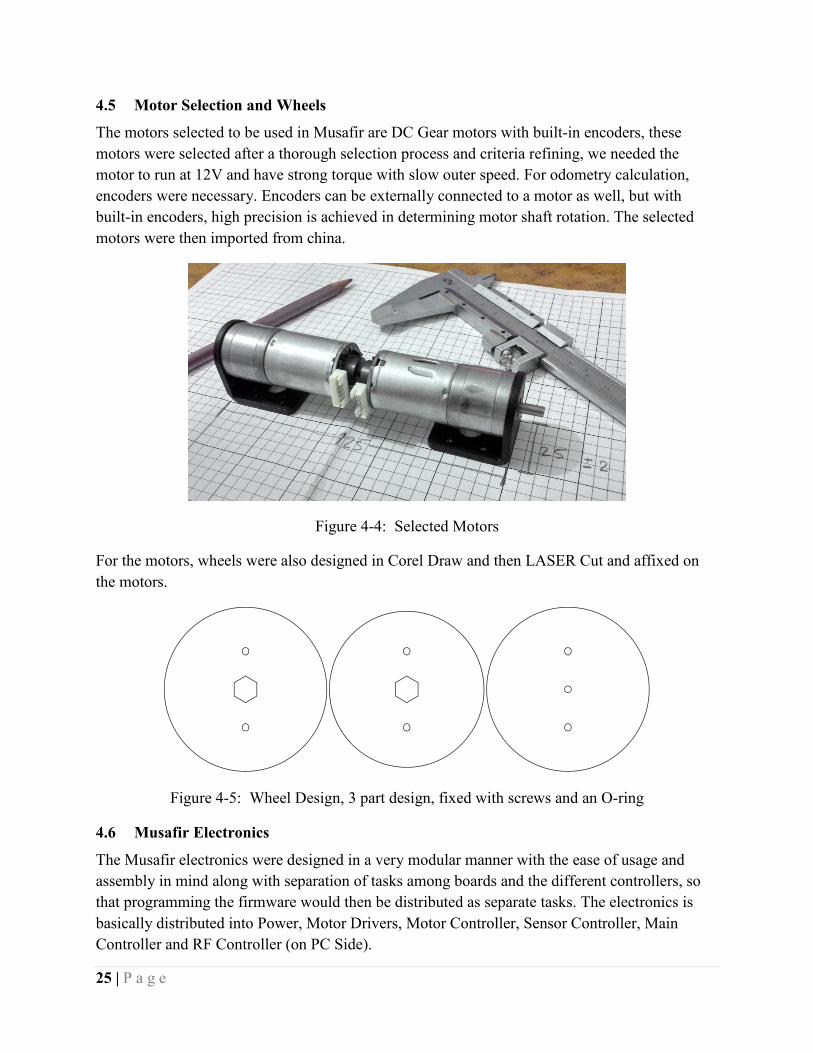
4.5 Motor Selection and Wheels

The motors selected to be used in Musafir are DC Gear motors with built-in encoders, these

motors were selected after a thorough selection process and criteria refining, we needed the

motor to run at 12V and have strong torque with slow outer speed. For odometry calculation,

encoders were necessary. Encoders can be externally connected to a motor as well, but with

built-in encoders, high precision is achieved in determining motor shaft rotation. The selected

motors were then imported from china.

Figure 4-4: Selected Motors

For the motors, wheels were also designed in Corel Draw and then LASER Cut and affixed on

the motors.

Figure 4-5: Wheel Design, 3 part design, fixed with screws and an O-ring

4.6 Musafir Electronics

The Musafir electronics were designed in a very modular manner with the ease of usage and

assembly in mind along with separation of tasks among boards and the different controllers, so

that programming the firmware would then be distributed as separate tasks. The electronics is

basically distributed into Power, Motor Drivers, Motor Controller, Sensor Controller, Main

Controller and RF Controller (on PC Side).

26 | P a g e

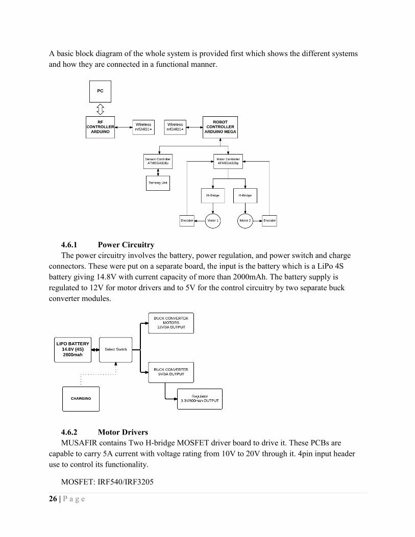
A basic block diagram of the whole system is provided

and how they are connected in a functional manner.

4.6.1 Power Circuitry

The power circuitry involves the battery, power regulation, and power switch and charge

connectors. These were put on a separate board, the input

battery giving 14.8V with current capacity of more than 2000mAh. The battery supply is

regulated to 12V for motor drivers and to 5V for the control circuitry by two separate buck

converter modules.

4.6.2 Motor Drivers

MUSAFIR contains Two H-bridge MOSFET driver board to drive it. These PCBs are

capable to carry 5A current with voltage rating from 10V to 20V through it. 4pin input header

use to control its functionality.

MOSFET: IRF540/IRF3205

A basic block diagram of the whole system is provided first which shows the different systems

and how they are connected in a functional manner.


connectors. These were put on a separate board, the input is the battery which is a LiPo 4S



bridge MOSFET driver board to drive it. These PCBs are


first which shows the different systems


is the battery which is a LiPo 4S



bridge MOSFET driver board to drive it. These PCBs are


27 | P a g e

MOSFET Driver: IR2104

4.6.3 Motor Controller Board

MUSAFIR contain the Motor Controller to control the motors. The separate PIDs has been

implemented to control the motors. The encoder has also been read by this motor controller to

control its close loop operation. Our motor controller is b

Mega board through serial communication. The predefined set of commands has been set up to

implement this communication. These command will be discussed later in section 4.7.

ontroller Board



control its close loop operation. Our motor controller is bound to take directions from on robot





ound to take directions from on robot



28 | P a g e

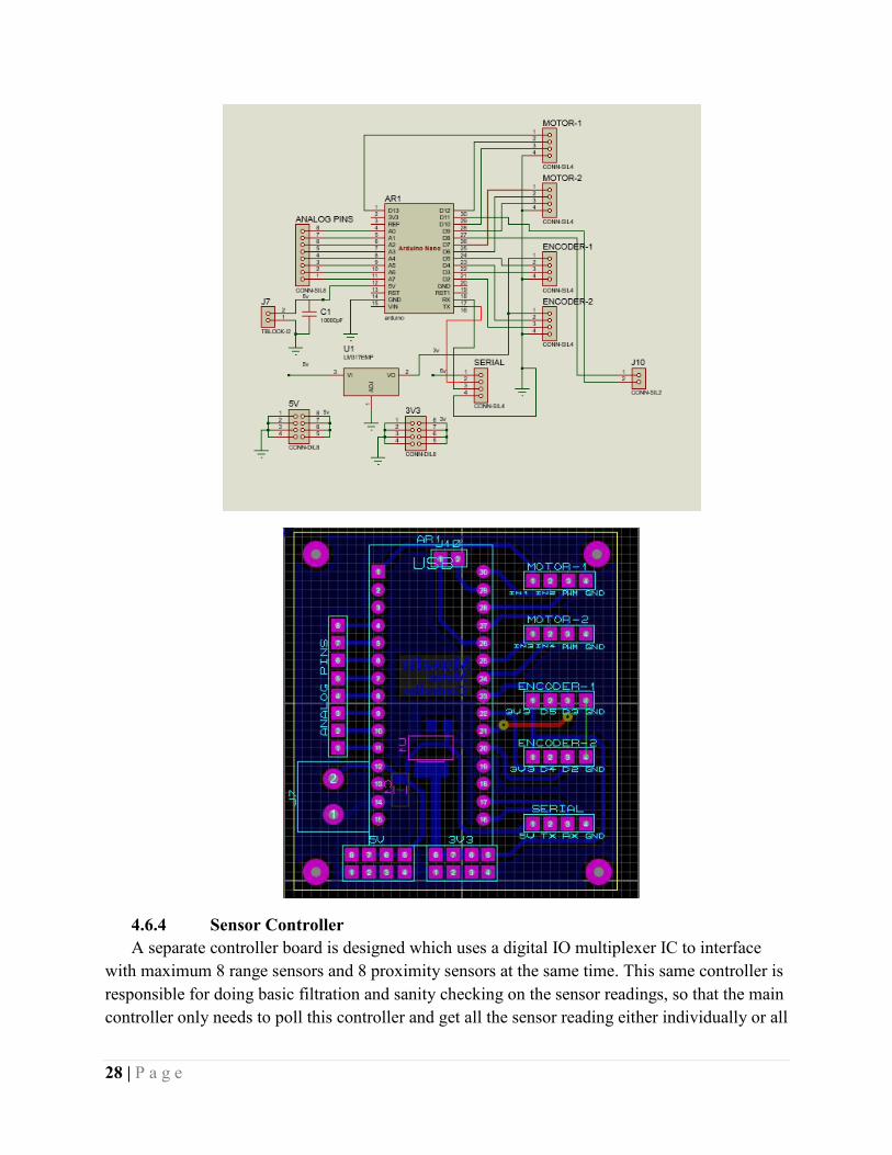
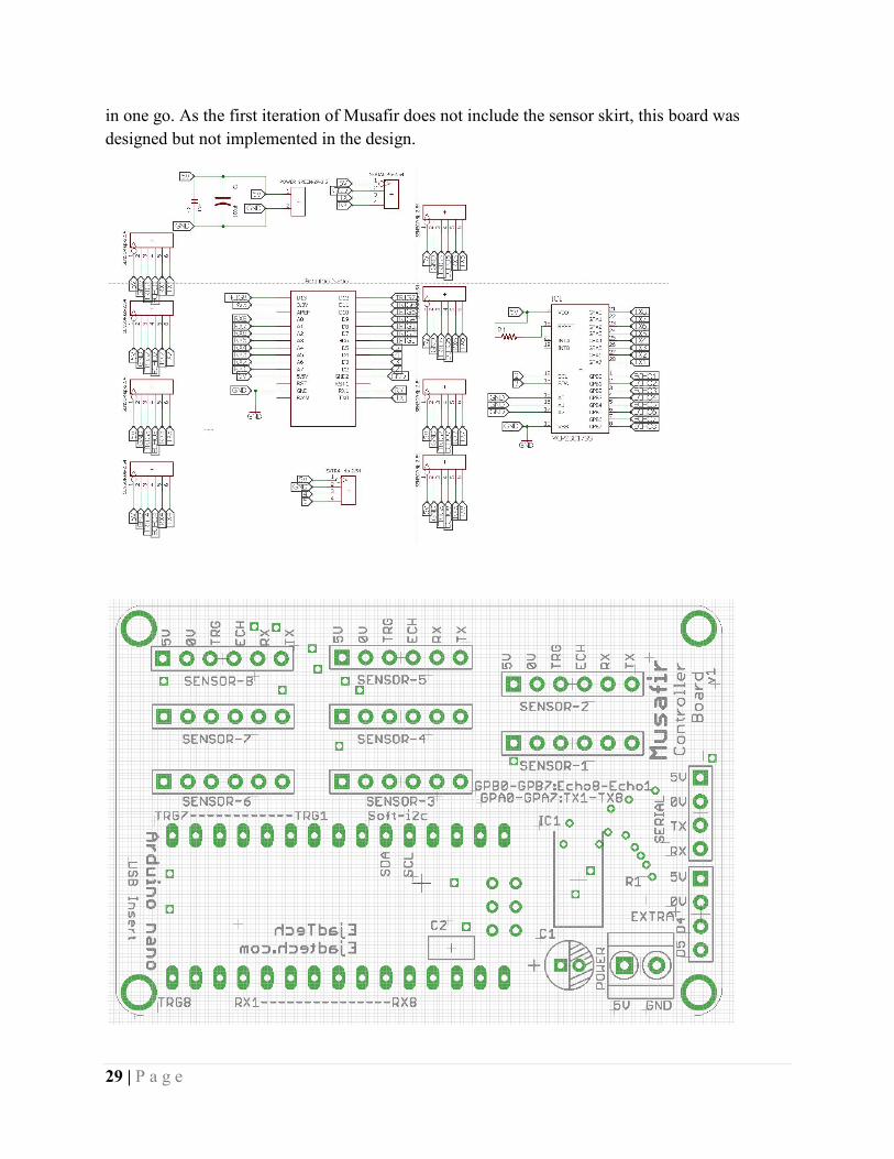
4.6.4 Sensor Controller

A separate controller board is designed which uses a digital IO multiplexer IC to interface

with maximum 8 range sensors and 8 proximity sensors at the same time. This same controller is

responsible for doing basic filtration and sanity checking on the sensor readings, so that the main

controller only needs to poll this controller and get all the sensor reading either individually or all

29 | P a g e

in one go. As the first iteration of Musafir does not include the sensor skirt, this board was

designed but not implemented in the design.


ed in the design.


30 | P a g e

4.6.5 Main Controller Board

Arduino Mega is used to control Musafir by taking directions wirelessly from PC to

implement the desired algorithm. Currently Mega is used for

Control the Motor controller.

Control the Sensor Controller

Communication through RF

Compute the IMU data.

So on Robot all the modules is in control of Arduino Mega.

4.6.6 RF Controller Board (PC Side)

RF control board is much similar to Main control borad except it does not have IMU. This board

is for sending the data packet of PC to Musafir or vice versa, through nrf24l01+ (Wireless

Communication Module).

Main Controller Board


implement the desired algorithm. Currently Mega is used for

Control the Motor controller.

Control the Sensor Controller

ation through RF

Compute the IMU data.

So on Robot all the modules is in control of Arduino Mega.

RF Controller Board (PC Side)


of PC to Musafir or vice versa, through nrf24l01+ (Wireless



of PC to Musafir or vice versa, through nrf24l01+ (Wireless

31 | P a g e

4.7 Musafir API and Control Methodologies

As the different controllers on the Musafir are responsible for their own separate tasks, we

developed an API, which is implemented

commands that it can handle. The main controller receives commands from the RF and then

sends the command to the appropriate controller.

For example, if MOTOR command is received, that is sent to the M

response of the Motor controller is then transmitted back via RF. Similar for Sensor command,

IMU command, etc.

A basic brief of the API is given below with the commands, the relevant paramters and the

response.

Command Description, Usage and Response

L

Motor PWM control, OPEN LOOPL,leftPWM,rightPWMResponse: l leftPWM and rightPWM are the speeds from 0 to 255, negative sign sets the direction.

D

Motor velocity Control ( mm/s ), close loopD,leftVelocity,rightVelocitResponse: d LeftVelocity and rightVelocity are the speeds from 0 to 800mm/s

M

Motor max Achievable PWMM,maxPWM,minPWM,1/2Response: m Motor Maximum and minimum PWM could be set through it. (left motor = 1, Right Motor=2)

R Read The Motor Encoder

Musafir API and Control Methodologies


developed an API, which is implemented on each controller and each controller responds to the


sends the command to the appropriate controller.

For example, if MOTOR command is received, that is sent to the Motor controller board and the



Description, Usage and Response Motor PWM control, OPEN LOOP L,leftPWM,rightPWM\n

leftPWM and rightPWM are the speeds from 0 to 255, negative sign sets the direction.Motor velocity Control ( mm/s ), close loop D,leftVelocity,rightVelocity\n

LeftVelocity and rightVelocity are the speeds from 0 to 800mm/s Motor max Achievable PWM M,maxPWM,minPWM,1/2\n

Motor Maximum and minimum PWM could be set through it. (left motor = 1, Right

Read The Motor Encoder


on each controller and each controller responds to the


otor controller board and the



leftPWM and rightPWM are the speeds from 0 to 255, negative sign sets the direction.

Motor Maximum and minimum PWM could be set through it. (left motor = 1, Right

32 | P a g e

R,1/2\n Response: r,leftMotorEncoder,rightMotorEncoder\n The motor controller will feedback the current encoder values

I

Reset Encoder I\n Response: i The encoder will then be set to zero

H

Set the PID parameters H,kp,ki,kd,1/2\n Response: h This command will set the PID values, (left motor = 1, Right Motor=2)

S

Read PID parameters S, 1/2\n Response: s,kp,ki,kd,1/2\n The motor controller will respond the current pid values of Desired Motor

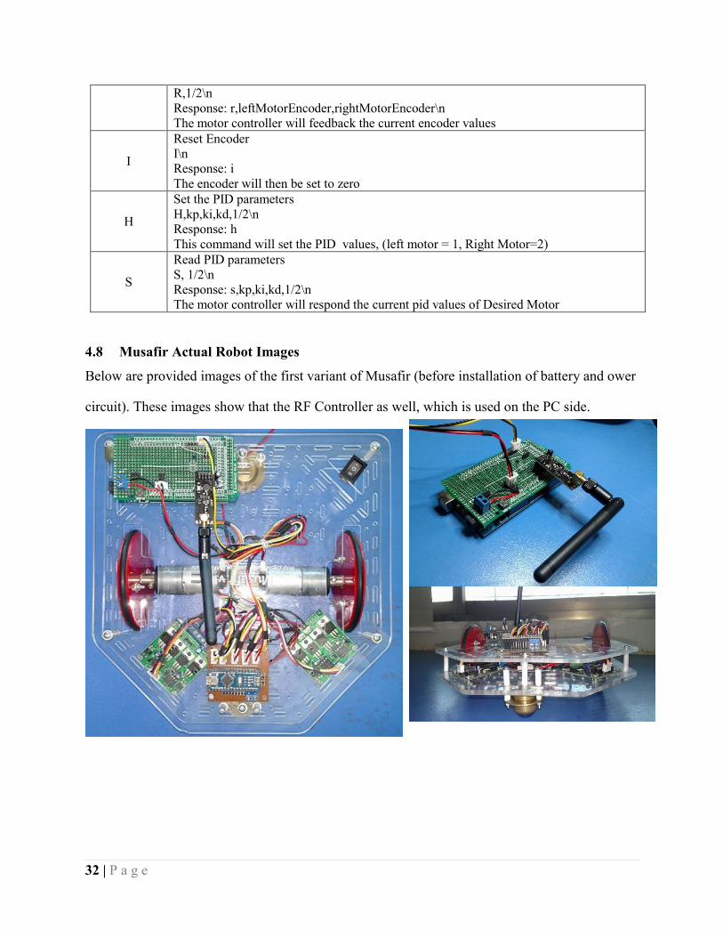
4.8 Musafir Actual Robot Images

Below are provided images of the first variant of Musafir (before installation of battery and ower

circuit). These images show that the RF Controller as well, which is used on the PC side.

33 | P a g e

Chapter 5. Testing Environment for MUSAFIR

When developing robotic control algorithms, the algorithms need to be tested very thoroughly,

analytical and completeness of the algorithm are tested by mathematical proofs, however until an

algorithm is tested in real world scenarios, it cannot be fully verified. However real world testing

requires design and development of hardware and also of test sites and test environments. There

is a middle ground testing of algorithms as well, which is physics simulation environments in

computers which test an algorithm by applying it on real world modeled 3d robots in a simulated

3d world with simulated physics.

Our process for testing of algorithms involves testing in MATLAB/Simulink environments,

where robots are treated as point-bots, then the same algorithm is tested with 3D simulation

software where real world 3d physics is applied. However, for actual testing of physical bots,

real world testing is necessary which is why we needed to design a lab test environment to allow

us to monitor and log the working of algorithms on actual robots.

5.1 Test Environment Setup

Our lab test environment consists of a camera and a computer which keep track of robot pose in

the lab test environment, such a setup allows to monitor the activity of the robots from a top-

view and the information is available for other software MATLAB/Simulink etc to determine the

next course of action for the robots.

The Test Environment also is useful as a way to measure the effectiveness of localization and

trajectory algorithms, by measuring the difference in pose of the robot as reported by running

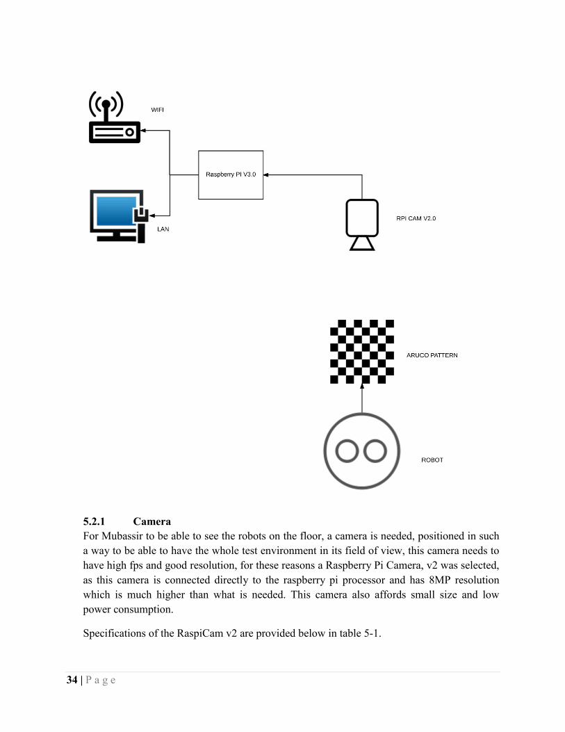
algorithm and from the test environment camera setup. A block diagram of the lab test setup is

provided below to show the main components of the test environment.

As this test environment is basically a system which is observing the robots move and for our

case, the robots are Musafir bots, the Test Environment System is named MUBASSIR, urdu for

observer.

5.2 Mubassir – Sub-Components

The lab test environment, Mubassir consists of mainly 3 components:

Camera

Computer System

Tags on Robots

34 | P a g e

5.2.1 Camera

For Mubassir to be able to see the robots on the floor, a camera is needed, positioned in such

a way to be able to have the whole test environment in its field of view, this camera needs to

have high fps and good resolutio

as this camera is connected directly to the raspberry pi processor and has 8MP resolution

which is much higher than what is needed. This camera also affords small size and low

power consumption.

Specifications of the RaspiCam v2 are provided below in table 5



have high fps and good resolution, for these reasons a Raspberry Pi Camera, v2 was selected,



Specifications of the RaspiCam v2 are provided below in table 5-1.



n, for these reasons a Raspberry Pi Camera, v2 was selected,



35 | P a g e

Lens Fixed focus Megapixels: 8 megapixel native resolution sensor Camera Resolution:

3280 x 2464 pixel stills

Video Resolution: 1080p30, 720p60 and 640x480p90 video Dimensions: 25mm x 23mm x 9mm Weight: ~3g Connector: ribbon connector Interface: CSI

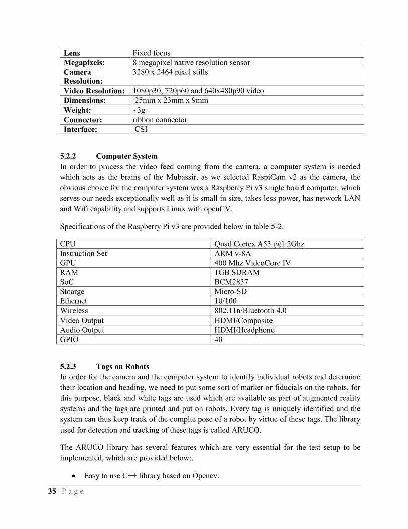
5.2.2 Computer System

In order to process the video feed coming from the camera, a computer system is needed

which acts as the brains of the Mubassir, as we selected RaspiCam v2 as the camera, the

obvious choice for the computer system was a Raspberry Pi v3 single board computer, which

serves our needs exceptionally well as it is small in size, takes less power, has network LAN

and Wifi capability and supports Linux with openCV.

Specifications of the Raspberry Pi v3 are provided below in table 5-2.

CPU Quad Cortex A53 @1.2Ghz Instruction Set ARM v-8A GPU 400 Mhz VideoCore IV RAM 1GB SDRAM SoC BCM2837 Stoarge Micro-SD Ethernet 10/100 Wireless 802.11n/Bluetooth 4.0 Video Output HDMI/Composite Audio Output HDMI/Headphone GPIO 40

5.2.3 Tags on Robots

In order for the camera and the computer system to identify individual robots and determine

their location and heading, we need to put some sort of marker or fiducials on the robots, for

this purpose, black and white tags are used which are available as part of augmented reality

systems and the tags are printed and put on robots. Every tag is uniquely identified and the

system can thus keep track of the complte pose of a robot by virtue of these tags. The library

used for detection and tracking of these tags is called ARUCO.

The ARUCO library has several features which are very essential for the test setup to be

implemented, which are provided below:.

Easy to use C++ library based on Opencv.

36 | P a g e

It can detect square planner marker from various libraries which having valid code

called dictionary.

Can determine pose of camera .

Integrated with OpenGL.

Fast, less computational cost, and cross platform.

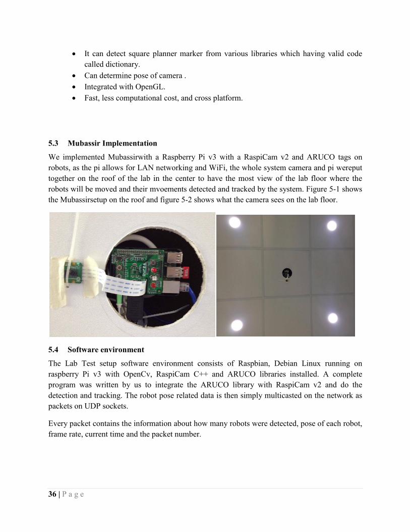
5.3 Mubassir Implementation

We implemented Mubassirwith a Raspberry Pi v3 with a RaspiCam v2 and ARUCO tags on

robots, as the pi allows for LAN networking and WiFi, the whole system camera and pi wereput

together on the roof of the lab in the center to have the most view of the lab floor where the

robots will be moved and their mvoements detected and tracked by the system. Figure 5-1 shows

the Mubassirsetup on the roof and figure 5-2 shows what the camera sees on the lab floor.

5.4 Software environment

The Lab Test setup software environment consists of Raspbian, Debian Linux running on

raspberry Pi v3 with OpenCv, RaspiCam C++ and ARUCO libraries installed. A complete

program was written by us to integrate the ARUCO library with RaspiCam v2 and do the

detection and tracking. The robot pose related data is then simply multicasted on the network as

packets on UDP sockets.

Every packet contains the information about how many robots were detected, pose of each robot,

frame rate, current time and the packet number.

37 | P a g e

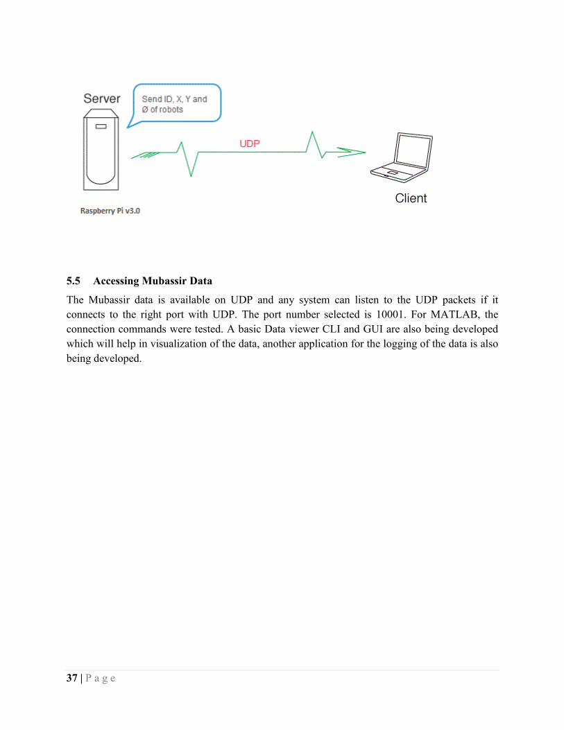
5.5 Accessing Mubassir Data

The Mubassir data is available on UDP and any system can listen to the UDP packets if it

connects to the right port with UDP. The port number selected is 10001. For MATLAB, the

connection commands were tested. A basic Data viewer CLI and GUI are also being developed

which will help in visualization of the data, another application for the logging of the data is also

being developed.

38 | P a g e

Chapter 6. Control Algorithm Development

6.1 Introduction

The basic objectives was to reproduce the results of the journal paper titled “A Decentralized Cooperative Control Scheme With Obstacle Avoidance for a Team of Mobile Robots” by Hamed Rezaee & Farzaneh Abdollahi.

It is worth mentioning that we didn’t have access to any of the materials (simulation or hardware) related to the aforementioned paper other than the paper itself.

First and foremost, Dynamical equation of the kth mobile robot is modeled and solved using

ode45 solver in MATLAB. The Electrostatic forces equation from (6) is substituted into

Equation (8) and the resultant is substituted into Equation (7). Finally, the dynamics and state of

the kth mobile robot in the proposed virtual structure is addressed. The algorithm has been tested

on a team of mobile robots having minimum of 3 robots to as much as 8 robots.

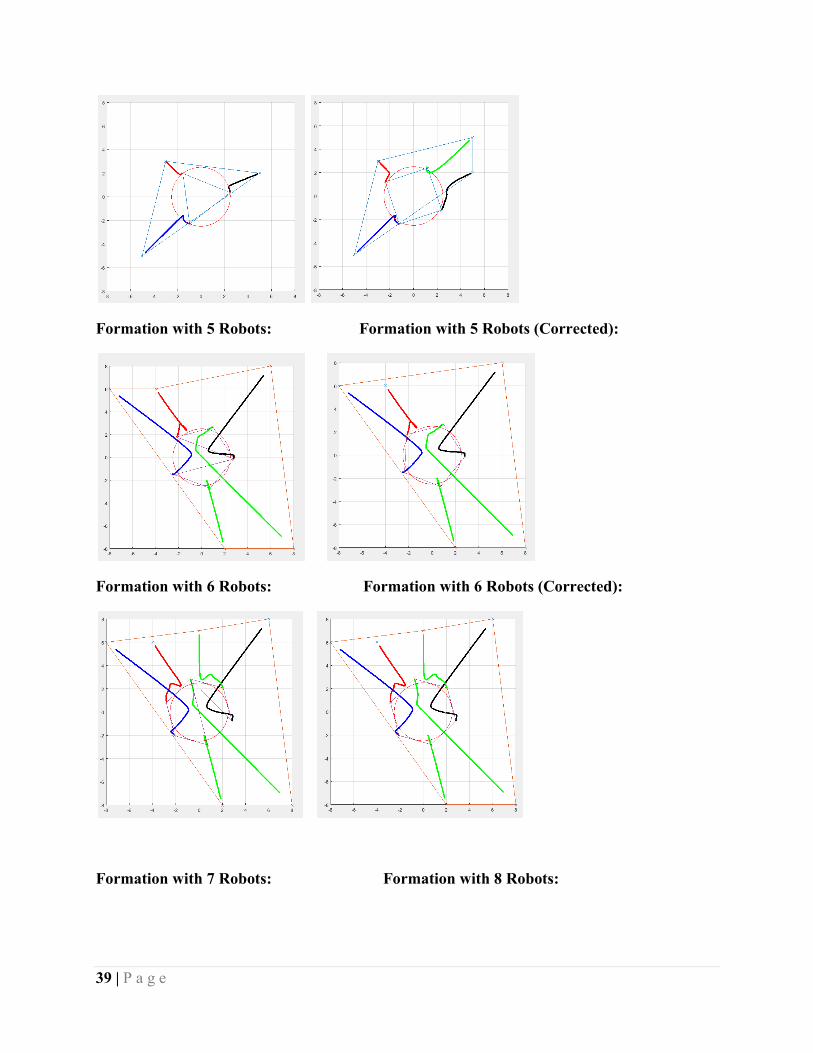
6.2 Simulation Results

Given the coordinates to four robots, the result

of formation algorithm is as follows:

Configuration Parameters: M = 1; (Mass of kth Robot) B = 1; Kd = 9; ksk = 1; kr = 0.15; alpha = 2; qk = 2.5; (Charges on kth Robot) K = 10; (Electrostatic Constant)

Formation with 3 Robots: Formation with 4Robots:

39 | P a g e

Formation with 5 Robots: Formation with 5 Robots (Corrected):

Formation with 6 Robots: Formation with 6 Robots (Corrected):

Formation with 7 Robots: Formation with 8 Robots:

40 | P a g e

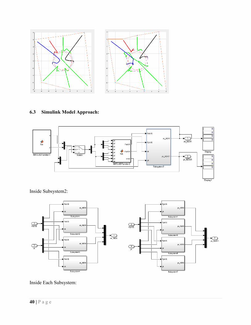
6.3 Simulink Model Approach:

Inside Subsystem2:

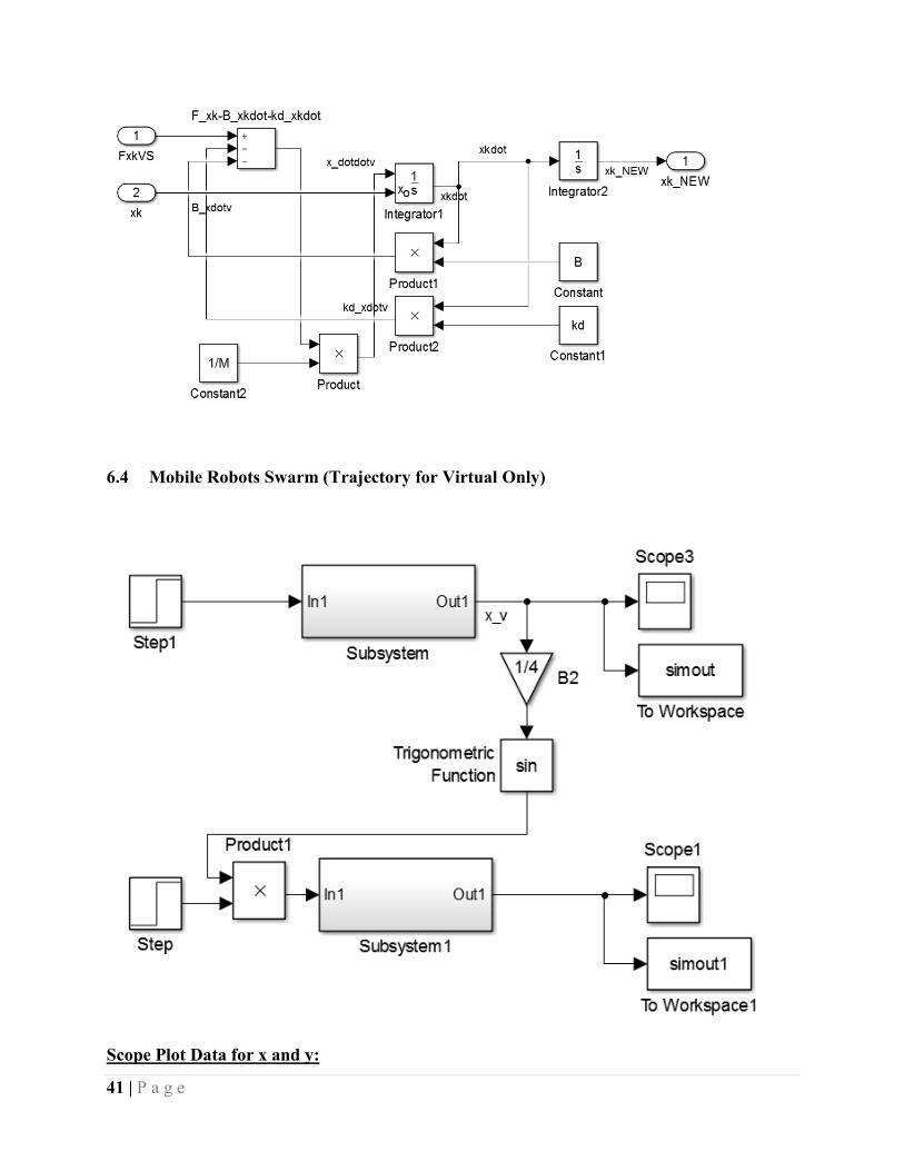
Inside Each Subsystem:

41 | P a g e

6.4 Mobile Robots Swarm (Trajectory for Virtual Only)

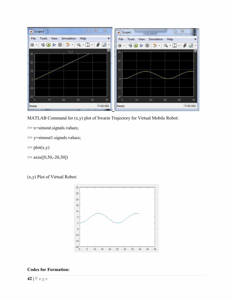
Scope Plot Data for x and y:

42 | P a g e

MATLAB Command for (x,y) plot of Swarm Trajectory for Virtual Mobile Robot:

>> x=simout.signals.values;

>> y=simout1.signals.values;

>> plot(x,y)

>> axis([0,50,-20,30])

(x,y) Plot of Virtual Robot:

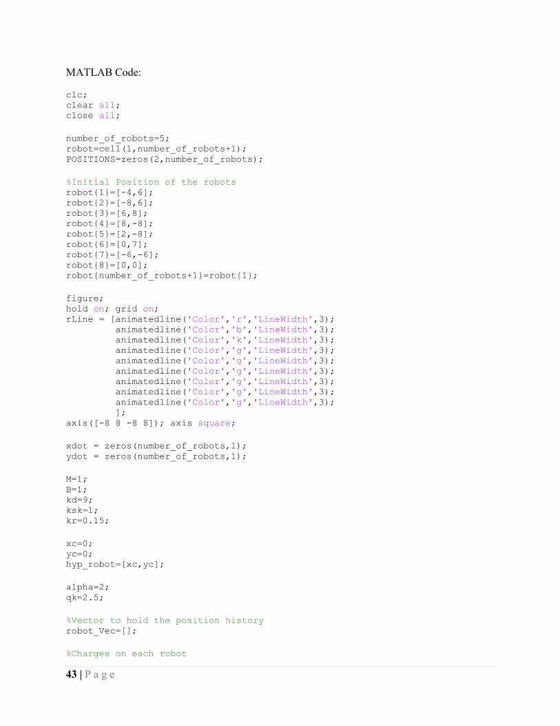
Codes for Formation:

43 | P a g e

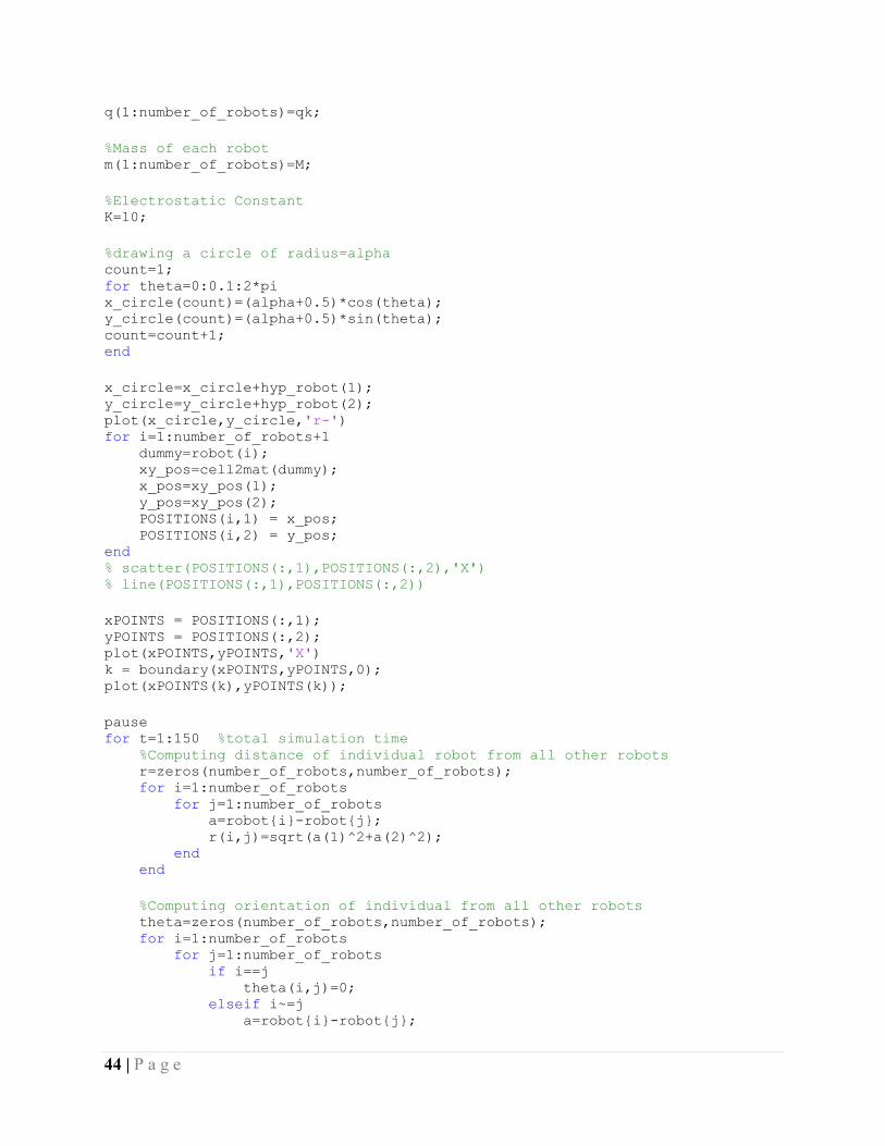
MATLAB Code:

clc; clear all; close all; number_of_robots=5; robot=cell(1,number_of_robots+1); POSITIONS=zeros(2,number_of_robots); %Initial Position of the robots robot{1}=[-4,6]; robot{2}=[-8,6]; robot{3}=[6,8]; robot{4}=[8,-8]; robot{5}=[2,-8]; robot{6}=[0,7]; robot{7}=[-6,-6]; robot{8}=[0,0]; robot{number_of_robots+1}=robot{1}; figure; hold on; grid on; rLine = [animatedline('Color','r','LineWidth',3); animatedline('Color','b','LineWidth',3); animatedline('Color','k','LineWidth',3); animatedline('Color','g','LineWidth',3); animatedline('Color','g','LineWidth',3); animatedline('Color','g','LineWidth',3); animatedline('Color','g','LineWidth',3); animatedline('Color','g','LineWidth',3); animatedline('Color','g','LineWidth',3); ]; axis([-8 8 -8 8]); axis square; xdot = zeros(number_of_robots,1); ydot = zeros(number_of_robots,1); M=1; B=1; kd=9; ksk=1; kr=0.15; xc=0; yc=0; hyp_robot=[xc,yc]; alpha=2; qk=2.5; %Vector to hold the position history robot_Vec=[]; %Charges on each robot

44 | P a g e

q(1:number_of_robots)=qk; %Mass of each robot m(1:number_of_robots)=M; %Electrostatic Constant K=10; %drawing a circle of radius=alpha count=1; for theta=0:0.1:2*pi x_circle(count)=(alpha+0.5)*cos(theta); y_circle(count)=(alpha+0.5)*sin(theta); count=count+1; end x_circle=x_circle+hyp_robot(1); y_circle=y_circle+hyp_robot(2); plot(x_circle,y_circle,'r-') for i=1:number_of_robots+1 dummy=robot(i); xy_pos=cell2mat(dummy); x_pos=xy_pos(1); y_pos=xy_pos(2); POSITIONS(i,1) = x_pos; POSITIONS(i,2) = y_pos; end % scatter(POSITIONS(:,1),POSITIONS(:,2),'X') % line(POSITIONS(:,1),POSITIONS(:,2)) xPOINTS = POSITIONS(:,1); yPOINTS = POSITIONS(:,2); plot(xPOINTS,yPOINTS,'X') k = boundary(xPOINTS,yPOINTS,0); plot(xPOINTS(k),yPOINTS(k)); pause for t=1:150 %total simulation time %Computing distance of individual robot from all other robots r=zeros(number_of_robots,number_of_robots); for i=1:number_of_robots for j=1:number_of_robots a=robot{i}-robot{j}; r(i,j)=sqrt(a(1)^2+a(2)^2); end end %Computing orientation of individual from all other robots theta=zeros(number_of_robots,number_of_robots); for i=1:number_of_robots for j=1:number_of_robots if i==j theta(i,j)=0; elseif i~=j a=robot{i}-robot{j};

45 | P a g e

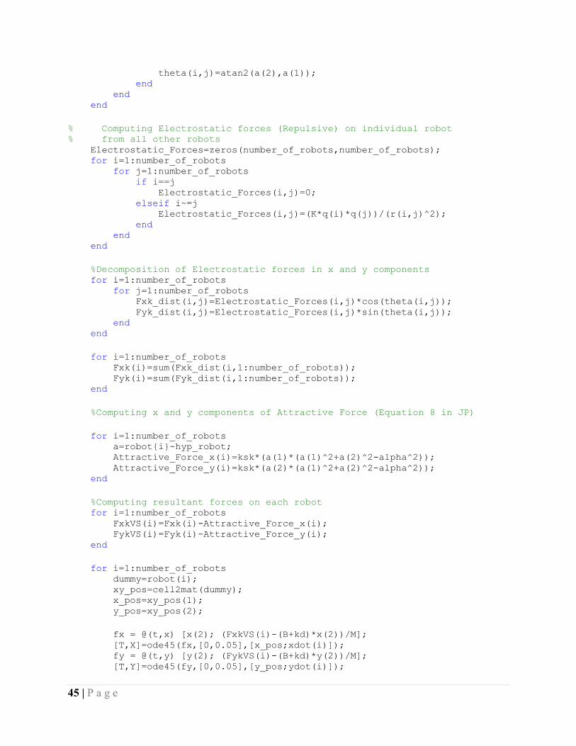
theta(i,j)=atan2(a(2),a(1)); end end end % Computing Electrostatic forces (Repulsive) on individual robot % from all other robots Electrostatic_Forces=zeros(number_of_robots,number_of_robots); for i=1:number_of_robots for j=1:number_of_robots if i==j Electrostatic_Forces(i,j)=0; elseif i~=j Electrostatic_Forces(i,j)=(K*q(i)*q(j))/(r(i,j)^2); end end end %Decomposition of Electrostatic forces in x and y components for i=1:number_of_robots for j=1:number_of_robots Fxk_dist(i,j)=Electrostatic_Forces(i,j)*cos(theta(i,j)); Fyk_dist(i,j)=Electrostatic_Forces(i,j)*sin(theta(i,j)); end end for i=1:number_of_robots Fxk(i)=sum(Fxk_dist(i,1:number_of_robots)); Fyk(i)=sum(Fyk_dist(i,1:number_of_robots)); end %Computing x and y components of Attractive Force (Equation 8 in JP) for i=1:number_of_robots a=robot{i}-hyp_robot; Attractive_Force_x(i)=ksk*(a(1)*(a(1)^2+a(2)^2-alpha^2)); Attractive_Force_y(i)=ksk*(a(2)*(a(1)^2+a(2)^2-alpha^2)); end %Computing resultant forces on each robot for i=1:number_of_robots FxkVS(i)=Fxk(i)-Attractive_Force_x(i); FykVS(i)=Fyk(i)-Attractive_Force_y(i); end for i=1:number_of_robots dummy=robot(i); xy_pos=cell2mat(dummy); x_pos=xy_pos(1); y_pos=xy_pos(2); fx = @(t,x) [x(2); (FxkVS(i)-(B+kd)*x(2))/M]; [T,X]=ode45(fx,[0,0.05],[x_pos;xdot(i)]); fy = @(t,y) [y(2); (FykVS(i)-(B+kd)*y(2))/M]; [T,Y]=ode45(fy,[0,0.05],[y_pos;ydot(i)]);

46 | P a g e

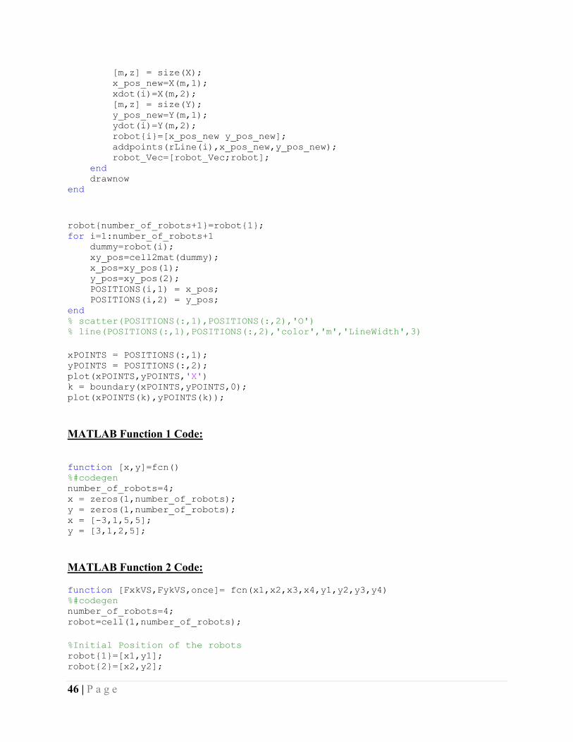
[m,z] = size(X); x_pos_new=X(m,1); xdot(i)=X(m,2); [m,z] = size(Y); y_pos_new=Y(m,1); ydot(i)=Y(m,2); robot{i}=[x_pos_new y_pos_new]; addpoints(rLine(i),x_pos_new,y_pos_new); robot_Vec=[robot_Vec;robot]; end drawnow end robot{number_of_robots+1}=robot{1}; for i=1:number_of_robots+1 dummy=robot(i); xy_pos=cell2mat(dummy); x_pos=xy_pos(1); y_pos=xy_pos(2); POSITIONS(i,1) = x_pos; POSITIONS(i,2) = y_pos; end % scatter(POSITIONS(:,1),POSITIONS(:,2),'O') % line(POSITIONS(:,1),POSITIONS(:,2),'color','m','LineWidth',3) xPOINTS = POSITIONS(:,1); yPOINTS = POSITIONS(:,2); plot(xPOINTS,yPOINTS,'X') k = boundary(xPOINTS,yPOINTS,0); plot(xPOINTS(k),yPOINTS(k));

MATLAB Function 1 Code:

function [x,y]=fcn() %#codegen number_of_robots=4; x = zeros(1,number_of_robots); y = zeros(1,number_of_robots); x = [-3,1,5,5]; y = [3,1,2,5];

MATLAB Function 2 Code:

function [FxkVS,FykVS,once]= fcn(x1,x2,x3,x4,y1,y2,y3,y4) %#codegen number_of_robots=4; robot=cell(1,number_of_robots); %Initial Position of the robots robot{1}=[x1,y1]; robot{2}=[x2,y2];

47 | P a g e

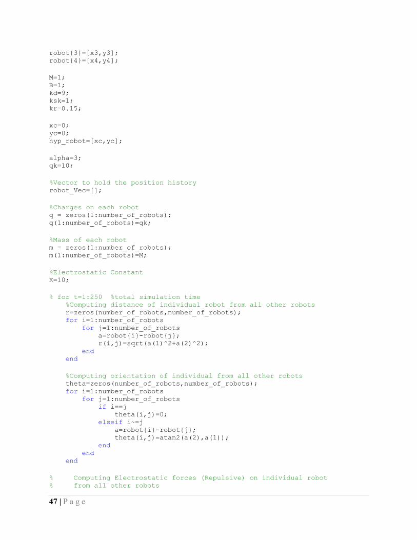
robot{3}=[x3,y3]; robot{4}=[x4,y4]; M=1; B=1; kd=9; ksk=1; kr=0.15; xc=0; yc=0; hyp_robot=[xc,yc]; alpha=3; qk=10; %Vector to hold the position history robot_Vec=[]; %Charges on each robot q = zeros(1:number_of_robots); q(1:number_of_robots)=qk; %Mass of each robot m = zeros(1:number_of_robots); m(1:number_of_robots)=M; %Electrostatic Constant K=10; % for t=1:250 %total simulation time %Computing distance of individual robot from all other robots r=zeros(number_of_robots,number_of_robots); for i=1:number_of_robots for j=1:number_of_robots a=robot{i}-robot{j}; r(i,j)=sqrt(a(1)^2+a(2)^2); end end %Computing orientation of individual from all other robots theta=zeros(number_of_robots,number_of_robots); for i=1:number_of_robots for j=1:number_of_robots if i==j theta(i,j)=0; elseif i~=j a=robot{i}-robot{j}; theta(i,j)=atan2(a(2),a(1)); end end end % Computing Electrostatic forces (Repulsive) on individual robot % from all other robots

48 | P a g e

Electrostatic_Forces=zeros(number_of_robots,number_of_robots); for i=1:number_of_robots for j=1:number_of_robots if i==j Electrostatic_Forces(i,j)=0; elseif i~=j Electrostatic_Forces(i,j)=(K*q(i)*q(j))/(r(i,j)^2); end end end Fxk_dist = zeros(number_of_robots,number_of_robots); Fyk_dist = zeros(number_of_robots,number_of_robots);

%Decomposition of Electrostatic forces in x and y components for i=1:number_of_robots for j=1:number_of_robots Fxk_dist(i,j)=Electrostatic_Forces(i,j)*cos(theta(i,j)); Fyk_dist(i,j)=Electrostatic_Forces(i,j)*sin(theta(i,j)); end end Fxk = zeros(1,number_of_robots); Fyk = zeros(1,number_of_robots); for i=1:number_of_robots Fxk(i)=sum(Fxk_dist(i,1:number_of_robots)); Fyk(i)=sum(Fyk_dist(i,1:number_of_robots)); end %Computing x and y components of Attractive Force (Equation 8 in JP) Attractive_Force_x = zeros(1,number_of_robots); Attractive_Force_y = zeros(1,number_of_robots); for i=1:number_of_robots a=robot{i}-hyp_robot; Attractive_Force_x(i)=ksk*(a(1)*(a(1)^2+a(2)^2-alpha^2)); Attractive_Force_y(i)=ksk*(a(2)*(a(1)^2+a(2)^2-alpha^2)); end FxkVS = zeros(1,number_of_robots); FykVS = zeros(1,number_of_robots); %Computing resultant forces on each robot for i=1:number_of_robots FxkVS(i)=Fxk(i)-Attractive_Force_x(i); FykVS(i)=Fyk(i)-Attractive_Force_y(i); end once = zeros(1,1); once = 3;

49 | P a g e

Chapter 7. Robot Localization by sensor fusion of GPS,

Odometer and INS

- Introduction:

This chapter discusses how data from three sensors namely INS (Inertial Navigation System),

GPS (Global Positioning System) and Odometer is combined to get accurate position of robot.

The data from these sensors is combined using sensor fusion scheme such as the Kalman Filter,

(KF) and weighting scheme.

Using the above mentioned sensor fusion scheme, the position of robot can be determined in

indoor as well as outdoor applications.

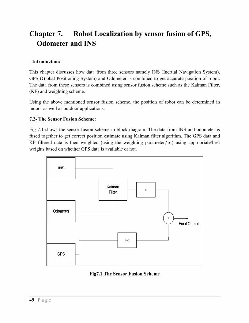
7.2- The Sensor Fusion Scheme:

Fig 7.1 shows the sensor fusion scheme in block diagram. The data from INS and odometer is

fused together to get correct position estimate using Kalman filter algorithm. The GPS data and

KF filtered data is then weighted (using the weighting parameter,‘α’) using appropriate/best

weights based on whether GPS data is available or not.

Fig7.1.The Sensor Fusion Scheme

50 | P a g e

7.3-Kalman Filter for Sensor Fusion:

The Kalman Filter is used to fuse the data from odometer and INS. Since the INS consists of

accelerometers and gyroscopes. Accelerometers data contains many kinds of errors such as bias

and random noise.

When the accelerometer data is double integrated to get position, there is error drift increasing

with time and produces wrong position results. Therefore, odometer position data is combined

with INS with Kalman filter to utilize the advantages of both the sensors and to get a correct

estimate of position.

Kalman Filter algorithm:

The Kalman Filter algorithm consists of the following steps:

1. Prediction and

2. Correction.

The algorithm consists of the following steps:

1. Set the initial values of states and error covariance

Matrix:

ˆ,xo Po

2. Predicting state and error covariance matrix.

1ˆ ˆ

k kx Ax

1T

k kP AP A Q

Where,

A is the state transition matrix or the system model and

Q is the process noise covariance matrix

3. Compute the Kalman Gain

1( )T TK K KK P H HP H R

Here,

H is the observation matrix

R is the measurement noise covariance matrix

51 | P a g e

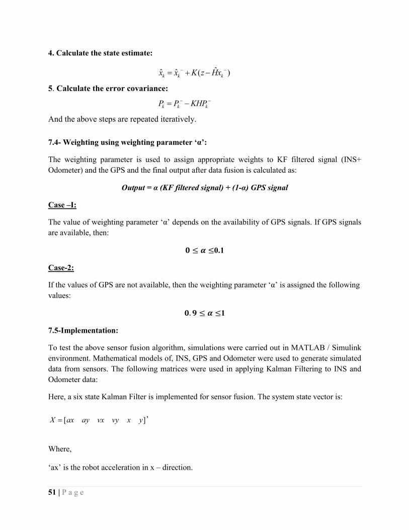
4. Calculate the state estimate:

ˆˆ ˆ ( )k k kx x K z Hx

5. Calculate the error covariance:

k k kP P KHP

And the above steps are repeated iteratively.

7.4- Weighting using weighting parameter ‘α’:

The weighting parameter is used to assign appropriate weights to KF filtered signal (INS+

Odometer) and the GPS and the final output after data fusion is calculated as:

Output = α (KF filtered signal) + (1-α) GPS signal

Case –I:

The value of weighting parameter ‘α’ depends on the availability of GPS signals. If GPS signals

are available, then:

� ≤ � ≤0.1

Case-2:

If the values of GPS are not available, then the weighting parameter ‘α’ is assigned the following

values:

�. � ≤ � ≤1

7.5-Implementation:

To test the above sensor fusion algorithm, simulations were carried out in MATLAB / Simulink

environment. Mathematical models of, INS, GPS and Odometer were used to generate simulated

data from sensors. The following matrices were used in applying Kalman Filtering to INS and

Odometer data:

Here, a six state Kalman Filter is implemented for sensor fusion. The system state vector is:

[ ]X ax ay vx vy x y ’

Where,

‘ax’ is the robot acceleration in x – direction.

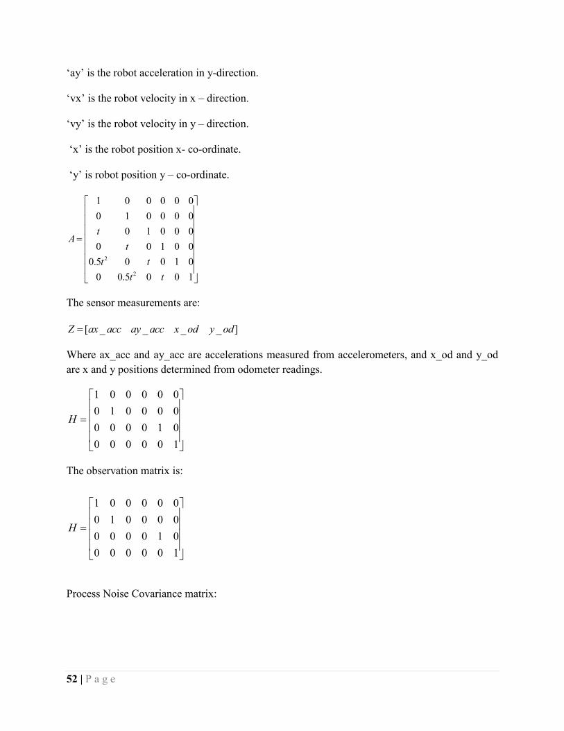
52 | P a g e

‘ay’ is the robot acceleration in y-direction.

‘vx’ is the robot velocity in x – direction.

‘vy’ is the robot velocity in y – direction.

‘x’ is the robot position x- co-ordinate.

‘y’ is robot position y – co-ordinate.

2

2

1 0 0 0 0 0

0 1 0 0 0 0

0 1 0 0 0

0 0 1 0 0

0.5 0 0 1 0

0 0.5 0 0 1

tA

t

t t

t t

The sensor measurements are:

[ _ _ _ _ ]Z ax acc ay acc x od y od

Where ax_acc and ay_acc are accelerations measured from accelerometers, and x_od and y_od

are x and y positions determined from odometer readings.

1 0 0 0 0 0

0 1 0 0 0 0

0 0 0 0 1 0

0 0 0 0 0 1

H

The observation matrix is:

1 0 0 0 0 0

0 1 0 0 0 0

0 0 0 0 1 0

0 0 0 0 0 1

H

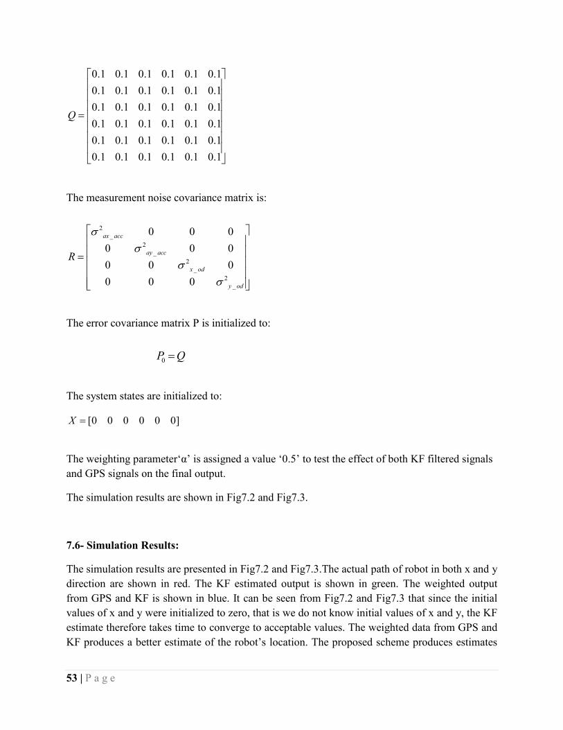
Process Noise Covariance matrix:

53 | P a g e

0.1 0.1 0.1 0.1 0.1 0.1

0.1 0.1 0.1 0.1 0.1 0.1

0.1 0.1 0.1 0.1 0.1 0.1

0.1 0.1 0.1 0.1 0.1 0.1

0.1 0.1 0.1 0.1 0.1 0.1

0.1 0.1 0.1 0.1 0.1 0.1

Q

The measurement noise covariance matrix is:

2_

2_

2_

2_

0 0 0

0 0 0

0 0 0

0 0 0

ax acc

ay acc

x od

y od

R

The error covariance matrix P is initialized to:

0P Q

The system states are initialized to:

[0 0 0 0 0 0]X

The weighting parameter‘α’ is assigned a value ‘0.5’ to test the effect of both KF filtered signals

and GPS signals on the final output.

The simulation results are shown in Fig7.2 and Fig7.3.

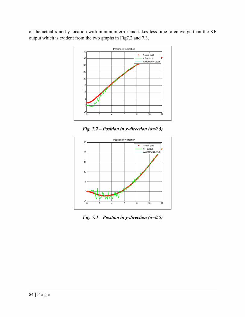
7.6- Simulation Results:

The simulation results are presented in Fig7.2 and Fig7.3.The actual path of robot in both x and y

direction are shown in red. The KF estimated output is shown in green. The weighted output

from GPS and KF is shown in blue. It can be seen from Fig7.2 and Fig7.3 that since the initial

values of x and y were initialized to zero, that is we do not know initial values of x and y, the KF

estimate therefore takes time to converge to acceptable values. The weighted data from GPS and

KF produces a better estimate of the robot’s location. The proposed scheme produces estimates

54 | P a g e

of the actual x and y location with minimum error and takes less time to converge than the KF

output which is evident from the two graphs in Fig7.2 and 7.3.

Fig. 7.2 – Position in x-direction (α=0.5)

Fig. 7.3 – Position in y-direction (α=0.5)

0 2 4 6 8 10 12-5

0

5

10

15

20

25

30

35

40Position in x-direction

Actual path

KF output

Weighted Output

0 2 4 6 8 10 12-5

0

5

10

15

20

25Position in y-direction

Actual path

KF output

Weighted Output

55 | P a g e

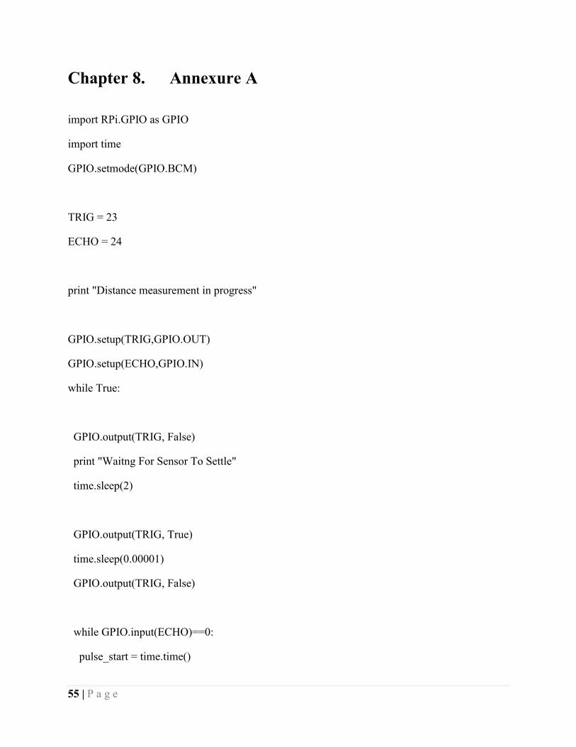
Chapter 8. Annexure A

import RPi.GPIO as GPIO

import time

GPIO.setmode(GPIO.BCM)

TRIG = 23

ECHO = 24

print "Distance measurement in progress"

GPIO.setup(TRIG,GPIO.OUT)

GPIO.setup(ECHO,GPIO.IN)

while True:

GPIO.output(TRIG, False)

print "Waitng For Sensor To Settle"

time.sleep(2)

GPIO.output(TRIG, True)

time.sleep(0.00001)

GPIO.output(TRIG, False)

while GPIO.input(ECHO)==0:

pulse_start = time.time()

56 | P a g e

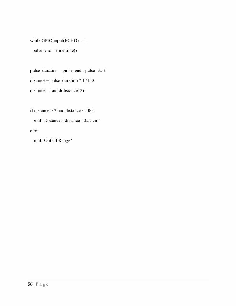
while GPIO.input(ECHO)==1:

pulse_end = time.time()

pulse_duration = pulse_end - pulse_start

distance = pulse_duration * 17150

distance = round(distance, 2)

if distance > 2 and distance < 400:

print "Distance:",distance - 0.5,"cm"

else:

print "Out Of Range"

57 | P a g e

Chapter 9. Annexure B

Main.h File

#ifndef MAINWINDOW_H

#define MAINWINDOW_H

#include <QMainWindow>

#include <QImage>

class QLabel;

class LeptonThread;

class QGridLayout;

class MainWindow : public QMainWindow {

Q_OBJECT

enum { ImageWidth = 320, ImageHeight = 240 };

static int snapshotCount;

QLabel *imageLabel;

LeptonThread *thread;

QGridLayout *layout;

unsigned short rawMin, rawMax;

58 | P a g e

QVector<unsigned short> rawData;

QImage rgbImage;

public:

explicit MainWindow(QWidget *parent = 0);

public slots:

void saveSnapshot();

void updateImage(unsigned short *, int, int);

};

#endif // MAINWINDOW_H

Main.cpp File

#include "mainwindow.h"

#include <QLabel>

#include <QPushButton>

#include <QGridLayout>

#include <QImage>

#include <QPixmap>

#include <QPainter>

#include <QFile>

#include "LeptonThread.h"

int MainWindow::snapshotCount = 0;

59 | P a g e

MainWindow::MainWindow(QWidget *parent)

: QMainWindow(parent)

, rawData(LeptonThread::FrameWords)

, rgbImage(LeptonThread::FrameWidth, LeptonThread::FrameHeight,

QImage::Format_RGB888)

{

QWidget *mainWidget = new QWidget();

setCentralWidget(mainWidget);

layout = new QGridLayout();

mainWidget->setLayout(layout);

imageLabel = new QLabel();

layout->addWidget(imageLabel, 0, 0, Qt::AlignCenter);

QPixmap filler(ImageWidth, ImageHeight); filler.fill(Qt::red);

imageLabel->setPixmap(filler);

thread = new LeptonThread();

connect(thread, SIGNAL(updateImage(unsigned short *,int,int)), this,

SLOT(updateImage(unsigned short *, int,int)));

60 | P a g e

//QPushButton *snapshotButton = new QPushButton("Snapshot");

//layout->addWidget(snapshotButton, 1, 0, Qt::AlignCenter);

//connect(snapshotButton, SIGNAL(clicked()), this, SLOT(saveSnapshot()));

thread->start();

}

// Rainbow: const int colormap[] = {1, 3, 74, 0, 3, 74, 0, 3, 75, 0, 3, 75, 0, 3, 76, 0, 3, 76, 0, 3, 77,

0, 3, 79, 0, 3, 82, 0, 5, 85, 0, 7, 88, 0, 10, 91, 0, 14, 94, 0, 19, 98, 0, 22, 100, 0, 25, 103, 0, 28,

106, 0, 32, 109, 0, 35, 112, 0, 38, 116, 0, 40, 119, 0, 42, 123, 0, 45, 128, 0, 49, 133, 0, 50, 134, 0,

51, 136, 0, 52, 137, 0, 53, 139, 0, 54, 142, 0, 55, 144, 0, 56, 145, 0, 58, 149, 0, 61, 154, 0, 63,

156, 0, 65, 159, 0, 66, 161, 0, 68, 164, 0, 69, 167, 0, 71, 170, 0, 73, 174, 0, 75, 179, 0, 76, 181, 0,

78, 184, 0, 79, 187, 0, 80, 188, 0, 81, 190, 0, 84, 194, 0, 87, 198, 0, 88, 200, 0, 90, 203, 0, 92,

205, 0, 94, 207, 0, 94, 208, 0, 95, 209, 0, 96, 210, 0, 97, 211, 0, 99, 214, 0, 102, 217, 0, 103, 218,

0, 104, 219, 0, 105, 220, 0, 107, 221, 0, 109, 223, 0, 111, 223, 0, 113, 223, 0, 115, 222, 0, 117,

221, 0, 118, 220, 1, 120, 219, 1, 122, 217, 2, 124, 216, 2, 126, 214, 3, 129, 212, 3, 131, 207, 4,

132, 205, 4, 133, 202, 4, 134, 197, 5, 136, 192, 6, 138, 185, 7, 141, 178, 8, 142, 172, 10, 144,

166, 10, 144, 162, 11, 145, 158, 12, 146, 153, 13, 147, 149, 15, 149, 140, 17, 151, 132, 22, 153,

120, 25, 154, 115, 28, 156, 109, 34, 158, 101, 40, 160, 94, 45, 162, 86, 51, 164, 79, 59, 167, 69,

67, 171, 60, 72, 173, 54, 78, 175, 48, 83, 177, 43, 89, 179, 39, 93, 181, 35, 98, 183, 31, 105, 185,

26, 109, 187, 23, 113, 188, 21, 118, 189, 19, 123, 191, 17, 128, 193, 14, 134, 195, 12, 138, 196,

10, 142, 197, 8, 146, 198, 6, 151, 200, 5, 155, 201, 4, 160, 203, 3, 164, 204, 2, 169, 205, 2, 173,

206, 1, 175, 207, 1, 178, 207, 1, 184, 208, 0, 190, 210, 0, 193, 211, 0, 196, 212, 0, 199, 212, 0,

202, 213, 1, 207, 214, 2, 212, 215, 3, 215, 214, 3, 218, 214, 3, 220, 213, 3, 222, 213, 4, 224, 212,

4, 225, 212, 5, 226, 212, 5, 229, 211, 5, 232, 211, 6, 232, 211, 6, 233, 211, 6, 234, 210, 6, 235,

210, 7, 236, 209, 7, 237, 208, 8, 239, 206, 8, 241, 204, 9, 242, 203, 9, 244, 202, 10, 244, 201, 10,

245, 200, 10, 245, 199, 11, 246, 198, 11, 247, 197, 12, 248, 194, 13, 249, 191, 14, 250, 189, 14,

251, 187, 15, 251, 185, 16, 252, 183, 17, 252, 178, 18, 253, 174, 19, 253, 171, 19, 254, 168, 20,

61 | P a g e

254, 165, 21, 254, 164, 21, 255, 163, 22, 255, 161, 22, 255, 159, 23, 255, 157, 23, 255, 155, 24,

255, 149, 25, 255, 143, 27, 255, 139, 28, 255, 135, 30, 255, 131, 31, 255, 127, 32, 255, 118, 34,

255, 110, 36, 255, 104, 37, 255, 101, 38, 255, 99, 39, 255, 93, 40, 255, 88, 42, 254, 82, 43, 254,

77, 45, 254, 69, 47, 254, 62, 49, 253, 57, 50, 253, 53, 52, 252, 49, 53, 252, 45, 55, 251, 39, 57,

251, 33, 59, 251, 32, 60, 251, 31, 60, 251, 30, 61, 251, 29, 61, 251, 28, 62, 250, 27, 63, 250, 27,

65, 249, 26, 66, 249, 26, 68, 248, 25, 70, 248, 24, 73, 247, 24, 75, 247, 25, 77, 247, 25, 79, 247,

26, 81, 247, 32, 83, 247, 35, 85, 247, 38, 86, 247, 42, 88, 247, 46, 90, 247, 50, 92, 248, 55, 94,

248, 59, 96, 248, 64, 98, 248, 72, 101, 249, 81, 104, 249, 87, 106, 250, 93, 108, 250, 95, 109,

250, 98, 110, 250, 100, 111, 251, 101, 112, 251, 102, 113, 251, 109, 117, 252, 116, 121, 252,

121, 123, 253, 126, 126, 253, 130, 128, 254, 135, 131, 254, 139, 133, 254, 144, 136, 254, 151,

140, 255, 158, 144, 255, 163, 146, 255, 168, 149, 255, 173, 152, 255, 176, 153, 255, 178, 155,

255, 184, 160, 255, 191, 165, 255, 195, 168, 255, 199, 172, 255, 203, 175, 255, 207, 179, 255,

211, 182, 255, 216, 185, 255, 218, 190, 255, 220, 196, 255, 222, 200, 255, 225, 202, 255, 227,

204, 255, 230, 206, 255, 233, 208};

const int colormap[] = {255, 255, 255, 253, 253, 253, 251, 251, 251, 249, 249, 249, 247, 247,

247, 245, 245, 245, 243, 243, 243, 241, 241, 241, 239, 239, 239, 237, 237, 237, 235, 235, 235,

233, 233, 233, 231, 231, 231, 229, 229, 229, 227, 227, 227, 225, 225, 225, 223, 223, 223, 221,

221, 221, 219, 219, 219, 217, 217, 217, 215, 215, 215, 213, 213, 213, 211, 211, 211, 209, 209,

209, 207, 207, 207, 205, 205, 205, 203, 203, 203, 201, 201, 201, 199, 199, 199, 197, 197, 197,

195, 195, 195, 193, 193, 193, 191, 191, 191, 189, 189, 189, 187, 187, 187, 185, 185, 185, 183,

183, 183, 181, 181, 181, 179, 179, 179, 177, 177, 177, 175, 175, 175, 173, 173, 173, 171, 171,

171, 169, 169, 169, 167, 167, 167, 165, 165, 165, 163, 163, 163, 161, 161, 161, 159, 159, 159,

157, 157, 157, 155, 155, 155, 153, 153, 153, 151, 151, 151, 149, 149, 149, 147, 147, 147, 145,

145, 145, 143, 143, 143, 141, 141, 141, 139, 139, 139, 137, 137, 137, 135, 135, 135, 133, 133,

133, 131, 131, 131, 129, 129, 129, 126, 126, 126, 124, 124, 124, 122, 122, 122, 120, 120, 120,

118, 118, 118, 116, 116, 116, 114, 114, 114, 112, 112, 112, 110, 110, 110, 108, 108, 108, 106,

106, 106, 104, 104, 104, 102, 102, 102, 100, 100, 100, 98, 98, 98, 96, 96, 96, 94, 94, 94, 92, 92,

92, 90, 90, 90, 88, 88, 88, 86, 86, 86, 84, 84, 84, 82, 82, 82, 80, 80, 80, 78, 78, 78, 76, 76, 76, 74,

74, 74, 72, 72, 72, 70, 70, 70, 68, 68, 68, 66, 66, 66, 64, 64, 64, 62, 62, 62, 60, 60, 60, 58, 58, 58,

56, 56, 56, 54, 54, 54, 52, 52, 52, 50, 50, 50, 48, 48, 48, 46, 46, 46, 44, 44, 44, 42, 42, 42, 40, 40,

40, 38, 38, 38, 36, 36, 36, 34, 34, 34, 32, 32, 32, 30, 30, 30, 28, 28, 28, 26, 26, 26, 24, 24, 24, 22,

22, 22, 20, 20, 20, 18, 18, 18, 16, 16, 16, 14, 14, 14, 12, 12, 12, 10, 10, 10, 8, 8, 8, 6, 6, 6, 4, 4, 4,

2, 2, 2, 0, 0, 0, 0, 0, 9, 2, 0, 16, 4, 0, 24, 6, 0, 31, 8, 0, 38, 10, 0, 45, 12, 0, 53, 14, 0, 60, 17, 0, 67,

19, 0, 74, 21, 0, 82, 23, 0, 89, 25, 0, 96, 27, 0, 103, 29, 0, 111, 31, 0, 118, 36, 0, 120, 41, 0, 121,

46, 0, 122, 51, 0, 123, 56, 0, 124, 61, 0, 125, 66, 0, 126, 71, 0, 127, 76, 1, 128, 81, 1, 129, 86, 1,

130, 91, 1, 131, 96, 1, 132, 101, 1, 133, 106, 1, 134, 111, 1, 135, 116, 1, 136, 121, 1, 136, 125, 2,

137, 130, 2, 137, 135, 3, 137, 139, 3, 138, 144, 3, 138, 149, 4, 138, 153, 4, 139, 158, 5, 139, 163,

5, 139, 167, 5, 140, 172, 6, 140, 177, 6, 140, 181, 7, 141, 186, 7, 141, 189, 10, 137, 191, 13, 132,

194, 16, 127, 196, 19, 121, 198, 22, 116, 200, 25, 111, 203, 28, 106, 205, 31, 101, 207, 34, 95,

209, 37, 90, 212, 40, 85, 214, 43, 80, 216, 46, 75, 218, 49, 69, 221, 52, 64, 223, 55, 59, 224, 57,

62 | P a g e

49, 225, 60, 47, 226, 64, 44, 227, 67, 42, 228, 71, 39, 229, 74, 37, 230, 78, 34, 231, 81, 32, 231,

85, 29, 232, 88, 27, 233, 92, 24, 234, 95, 22, 235, 99, 19, 236, 102, 17, 237, 106, 14, 238, 109,

12, 239, 112, 12, 240, 116, 12, 240, 119, 12, 241, 123, 12, 241, 127, 12, 242, 130, 12, 242, 134,

12, 243, 138, 12, 243, 141, 13, 244, 145, 13, 244, 149, 13, 245, 152, 13, 245, 156, 13, 246, 160,

13, 246, 163, 13, 247, 167, 13, 247, 171, 13, 248, 175, 14, 248, 178, 15, 249, 182, 16, 249, 185,

18, 250, 189, 19, 250, 192, 20, 251, 196, 21, 251, 199, 22, 252, 203, 23, 252, 206, 24, 253, 210,

25, 253, 213, 27, 254, 217, 28, 254, 220, 29, 255, 224, 30, 255, 227, 39, 255, 229, 53, 255, 231,

67, 255, 233, 81, 255, 234, 95, 255, 236, 109, 255, 238, 123, 255, 240, 137, 255, 242, 151, 255,

244, 165, 255, 246, 179, 255, 248, 193, 255, 249, 207, 255, 251, 221, 255, 253, 235, 255, 255,

24};

void MainWindow::updateImage(unsigned short *data, int minValue, int maxValue){

// Record the raw data and min/max values

memcpy(&rawData[0], data, 2*LeptonThread::FrameWords);

rawMin = minValue; rawMax = maxValue;

// Map "rawData" to rgb values in "rgbImage" via the colormap

int diff = maxValue - minValue + 1;

for (int y = 0; y < LeptonThread::FrameHeight; ++y) {

for (int x = 0; x < LeptonThread::FrameWidth; ++x) {

int baseValue = rawData[LeptonThread::FrameWidth*y + x]; // take input value in [0,

65536)

int scaledValue = 256*(baseValue - minValue)/diff; // map value to interval [0, 256), and

set the pixel to its color value above

rgbImage.setPixel(x, y, qRgb(colormap[3*scaledValue], colormap[3*scaledValue+1],

colormap[3*scaledValue+2]));

}

}

// Update the on-screen image

63 | P a g e

QPixmap pixmap = QPixmap::fromImage(rgbImage).scaled(ImageWidth, ImageHeight,

Qt::KeepAspectRatio);

QPainter painter(&pixmap);

// ... mark up pixmap, if so desired

imageLabel->setPixmap(pixmap);

saveSnapshot();

}

void MainWindow::saveSnapshot() {

usleep(2000000);

++snapshotCount;

// Raw file format: binary, one word for min value, one for max value, then 80*60 words of

raw data

QFile rawFile(QString("raw%1.bin").arg(snapshotCount));

rawFile.open(QIODevice::Truncate | QIODevice::ReadWrite);

QDataStream rawOut(&rawFile);

rawOut << rawMin << rawMax;

rawOut.writeRawData((char *) &rawData[0], 2*rawData.size());

rawFile.close();

// JPG image, top quality

rgbImage.save(QString("rgb%1.jpg").arg(snapshotCount), "JPG", 100);

}

64 | P a g e

Chapter 10. Annexure C

# program to take a series of pictures

import os

import string

import datetime

import time

from threading import Thread

first_pic = "fswebcam --device /dev/video0 -r 640x480 --no-banner /home/pi/test0.jpg"

second_pic = "fswebcam --device /dev/video1 -r 640x480 --no-banner /home/pi/test2.jpg"

ii = "0"

jj = "2"

aa = "test"

def picfun():

os.system(first_pic)

os.system(second_pic)

t=5 # initialise the pause between pictures in seconds

count=10 # initialise the number of pictures to be taken

i=1 # initialise (reset) the counting sequence

totalTime=(t*count) # Calculate the time in seconds

# Take a series of pictures one every t seconds

while(i<count):

leftTimeH = 0

leftTimeM = 0

leftTimeS = 0

65 | P a g e

# taking a picture by calling a command line prompt

x = Thread(target = picfun)

x.start()

totalTime = (t*(count-i)) # Calculate the time in seconds

print(i) # print the current count value to show progress

while(totalTime>=3600):

leftTimeH = leftTimeH + 1

totalTime = totaTime-3600

while(totalTime>=60):

leftTimeM = leftTimeM + 1

totalTime = totaTime-60

leftTimeS = totalTime

percentDone = (( i / count ) * 100)

percentDone = round(percentDone,2)

message1 = ("Time left to finish " +repr(leftTimeH) +" Hours " + repr(leftTimeM) + "

Minutes and " + repr(leftTimeS) + "Seconds")

message2 = (" "+repr(percentDone) + " %Completed! ")

print(message1)

print(message2)

i = i+1

if(i>count): # leave the loop when count fulfilled (not really necessary)

break

time.sleep(t) # wait the defined time t(s) between pictures

bb = "test" + ii

ii = int(ii)

66 | P a g e

ii = ii + 1

ii = str(ii)

first_pic = string.replace(first_pic, bb, aa+ii)

cc = "test" + jj

jj = int(jj)

jj = jj + 1

jj = str(jj)

second_pic = string.replace(second_pic, cc, aa+jj)

print("Finished!") # print to show when finished

Documents

Design and development of Intelligent Mobile Robots (IMRs ...pafkiet.edu.pk/main/wp-content/uploads/2016/09/Second-Deliverable... · Design and development of Intelligent Mobile Robots