Embed Size (px)
Citation preview
Calhoun: The NPS Institutional Archive
Theses and Dissertations Thesis Collection
2008-09
Design and implementation of an active calibration
system for weather radars
Phillips, Jason M.
Monterey California. Naval Postgraduate School
http://hdl.handle.net/10945/3977
NAVAL
POSTGRADUATE SCHOOL
MONTEREY, CALIFORNIA
THESIS
Approved for public release; distribution is unlimited
DESIGN AND IMPLEMENTATION OF AN ACTIVE CALIBRATION SYSTEM FOR WEATHER RADARS
by
Jason M. Phillips
September 2008
Thesis Advisor: Jeffrey B. Knorr Co-Advisor: Terry E. Smith

THIS PAGE INTENTIONALLY LEFT BLANK
i
REPORT DOCUMENTATION PAGE Form Approved OMB No. 0704-0188 Public reporting burden for this collection of information is estimated to average 1 hour per response, including the time for reviewing instruction, searching existing data sources, gathering and maintaining the data needed, and completing and reviewing the collection of information. Send comments regarding this burden estimate or any other aspect of this collection of information, including suggestions for reducing this burden, to Washington headquarters Services, Directorate for Information Operations and Reports, 1215 Jefferson Davis Highway, Suite 1204, Arlington, VA 22202-4302, and to the Office of Management and Budget, Paperwork Reduction Project (0704-0188) Washington DC 20503. 1. AGENCY USE ONLY (Leave blank)
2. REPORT DATE September 2008
3. REPORT TYPE AND DATES COVERED Master’s Thesis
4. TITLE AND SUBTITLE Design and Implementation of an Active Calibration System for Weather Radars 6. AUTHOR(S) Jason M. Phillips
5. FUNDING NUMBERS
7. PERFORMING ORGANIZATION NAME(S) AND ADDRESS(ES) Naval Postgraduate School Monterey, CA 93943-5000
8. PERFORMING ORGANIZATION REPORT NUMBER
9. SPONSORING /MONITORING AGENCY NAME(S) AND ADDRESS(ES) N/A
10. SPONSORING/MONITORING AGENCY REPORT NUMBER
11. SUPPLEMENTARY NOTES The views expressed in this thesis are those of the author and do not reflect the official policy or position of the Department of Defense or the U.S. Government. 12a. DISTRIBUTION / AVAILABILITY STATEMENT Approved for public release; distribution is unlimited
12b. DISTRIBUTION CODE
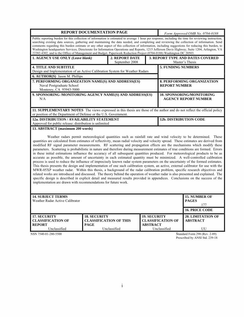
13. ABSTRACT (maximum 200 words) Weather radars permit meteorological quantities such as rainfall rate and wind velocity to be determined. These
quantities are calculated from estimates of reflectivity, mean radial velocity and velocity spread. These estimates are derived from modified RF signal parameter measurements. RF scattering and propagation effects are the mechanisms which modify these parameters. Scattering is probabilistic in nature and therefore during measurement estimates of true conditions are formed. Errors in these initial estimations influence the accuracy of all subsequent quantities produced. For meteorological products to be as accurate as possible, the amount of uncertainty in each estimated quantity must be minimized. A well-controlled calibration process is used to reduce the influence of imprecisely known radar system parameters on the uncertainty of the formed estimates. This thesis presents the design and implementation of one such calibration system, an active, external calibrator for use with the MWR-05XP weather radar. Within this thesis, a background of the radar calibration problem, specific research objectives and related works are introduced and discussed. The theory behind the operation of weather radar is also presented and explained. The specific design is described in explicit detail and measured results provided in appendices. Conclusions on the success of the implementation are drawn with recommendations for future work.
15. NUMBER OF PAGES
177
14. SUBJECT TERMS Weather Radar Active Calibrator
16. PRICE CODE
17. SECURITY CLASSIFICATION OF REPORT
Unclassified
18. SECURITY CLASSIFICATION OF THIS PAGE
Unclassified
19. SECURITY CLASSIFICATION OF ABSTRACT
Unclassified
20. LIMITATION OF ABSTRACT
UU NSN 7540-01-280-5500 Standard Form 298 (Rev. 2-89) Prescribed by ANSI Std. 239-18

ii
THIS PAGE INTENTIONALLY LEFT BLANK
iii
Approved for public release; distribution is unlimited
DESIGN AND IMPLEMENTATION OF AN ACTIVE CALIBRATION SYSTEM FOR WEATHER RADARS
Jason M. Phillips
Civilian, United States Department of Defense B.S.E.E., University of Maryland - College Park, 2002
B.S. Mathematics, University of Maryland - College Park, 2002
Submitted in partial fulfillment of the requirements for the degrees of
MASTER OF SCIENCE IN ELECTRICAL ENGINEERING
MASTER OF SCIENCE IN ELECTRONIC WARFARE SYSTEMS ENGINEERING
from the
NAVAL POSTGRADUATE SCHOOL September 2008
Author: Jason M. Phillips
Approved by: Jeffrey B. Knorr Thesis Advisor
Terry E. Smith Co-Advisor
Jeffrey B. Knorr Chairman, Department of Electrical and Computer Engineering Dan C. Boger Chairman, Department of Information Sciences

iv
THIS PAGE INTENTIONALLY LEFT BLANK
v
ABSTRACT
Pulsed weather radars can be used to depict meteorological conditions such as
rainfall rate and wind velocity. These quantities are calculated from measurements of
reflectivity, mean radial velocity and velocity spread using echo signal samples from
weather targets. These radar measurements derive from modified radio frequency (RF)
echo signal parameters, including amplitude, frequency and phase, returned to the radar
from the weather target. RF scattering and propagation effects modify echo signal
parameters. Bias and variance in the weather signal parameter estimates naturally
influence the accuracy of all subsequent quantities produced. For meteorological
products to be as accurate as possible, the amount of uncertainty in each estimated
quantity must be minimized. If radar system parameters are not accurately known, the
reflectivity estimate will be biased. A well-controlled calibration process is therefore
critical to reduce the bias of the reflectivity estimate. This thesis presents the design and
implementation of one such calibration system, specifically for use with the MWR-05XP
(a Mobile Phased-Array Pulse-Doppler X-band Weather Radar first created at the Naval
Postgraduate School in 2005), although the general results are applicable to all radars.
The calibration system presented is an active, external calibrator intended to verify end-
to-end radar system performance. Within this thesis, a background of the radar
calibration problem along with the research objectives for this specific project and related
works are introduced and discussed. The theory behind the operation of weather radar
(how the three principle quantities are measured and related to signal parameters) is also
presented and explained. The density function for precipitation, relation between signal
correlation and velocity spread, and fundamentals of weather radar signal parameter
estimation are given. The specific design is described in explicit detail and measured
results provided in appendices. Conclusions on the success of the implementation are
drawn and recommendations for future work are presented.

vi
THIS PAGE INTENTIONALLY LEFT BLANK
vii
TABLE OF CONTENTS
I. INTRODUCTION........................................................................................................1 A. BACKGROUND ..............................................................................................1 B. RESEARCH OBJECTIVE .............................................................................1 C. RELATED WORK ..........................................................................................3 D. ORGANIZATION OF THE THESIS............................................................5
II. BACKGROUND AND SUPPORTING THEORY...................................................7 A. WEATHER RADAR VS. TRADITIONAL RADAR...................................7 B. RADAR RESOLUTION CELL......................................................................8 C. SWERLING TARGET TYPES......................................................................9 D. SAMPLE CORRELATION..........................................................................10 E. ESTIMATION OF POWER DENSITY AND REFLECTIVITY (Z).......12
1. Antenna Gain and Beam effective Solid Angle ...............................12 2. Physics of Precipitation .....................................................................13
a. Size and Shape ........................................................................13 b. Drop Size Distribution (DSD).................................................14 c. Rainfall Rate ...........................................................................14
3. Weather Radar Range Equation and Estimation of Reflectivity ..15 F. RADAR PRINCIPLES AND WEATHER RADAR EQUATION
CORRECTION..............................................................................................16 G. ESTIMATION OF VELOCITY...................................................................19 H. ESTIMATION OF VELOCITY SPREAD..................................................20 I. CALIBRATION REQUIREMENTS...........................................................20 J. CALIBRATION METHODS AND SELECTED METHOD ....................21 K. SUMMARY ....................................................................................................22
III. DESIGN, IMPLEMENTATION AND OPERATION ...........................................23 A. DESIGN ..........................................................................................................23 B. HARDWARE IMPLEMENTATION ..........................................................24
1. System Description Overview ...........................................................24 2. Hardware List ....................................................................................25 3. Voltage Regulator Circuit .................................................................25 4. RF Components..................................................................................26 5. Control Hardware..............................................................................26 6. Hardware Limitations .......................................................................27
C. ACS FREQUENCY/DOPPLER CALIBRATION AND SOFTWARE IMPLEMENTATION ...................................................................................28
D. ADDING VELOCITY SPREAD..................................................................31 E. ACS AMPLITUDE/REFLECTIVITY CALIBRATION...........................31
1. Measurement Premise .......................................................................32 2. Measurement Method........................................................................33
a. Initial Calculations .................................................................34 b. Anechoic Chamber Measurements ........................................37
viii
IV. CONCLUSION AND FUTURE WORK .................................................................47 A. CONCLUSION ..............................................................................................47 B. FUTURE WORK...........................................................................................48
APPENDIX A. ACS PICTURES ................................................................................53
APPENDIX B. DIGITAL PHASE SHIFTER DATA...............................................65
APPENDIX C. SCALAR AND VECTOR NETWORK ANALYZER MEASUREMENT DATA .........................................................................................67
APPENDIX D. PROGRAMMABLE ATTENUATOR DATA ................................85
APPENDIX E. ANTENNA DATA .............................................................................87
APPENDIX F. ANTENNA PATTERN DATA .........................................................95 A. VNA ANTENNA PATTERN DATA............................................................95 B. ACS ANTENNA PATTERN DATA ..........................................................101 C. MATLAB PLOTTING FILES ...................................................................106 D. ABSOLUTE GAIN AND 3 DB BEAMWIDTH FOR X-BAND AND
PASTERNACK HORN ANTENNAS (CALCULATIONS AND MEASUREMENTS) ....................................................................................110
E. EXPLANATION OF DATAFILE MEASUREMENTS AND CALCULATIONS .......................................................................................114
F. ANTENNA ISOLATION TEST DATA ....................................................116
APPENDIX G. ANECHOIC CHAMBER................................................................119
APPENDIX H. COMPACTRIO ...............................................................................121 A. COMPACTRIO REAL-TIME EMBEDDED CONTROLLER (NI
CRIO-9004, 64/512 MEMORY) .................................................................121 B. COMPACTRIO RECONFIGURABLE EMBEDDED CHASSIS (NI
CRIO-9101, 1M GATE 4-SLOT CHASSIS) .............................................124 C. COMPACTRIO I/O MODULES FOR DIGITAL INPUT AND
COUNTER/TIMER (NI 9401, 8 CH 5 V/TTL HIGH SPEED BIDIRECTIONAL DIGITAL I/O MODULE) .........................................126
D. NI DEVELOPER SUITE WITH REAL-TIME AND FPGA SOFTWARE FOR COMPACTRIO..........................................................128
APPENDIX I. LABVIEW FOR THE DIGITAL PHASE SHIFTER ..................129 A. PHASESHIFTERCONTROL ....................................................................129 B. SLAVECONTROL......................................................................................130 C. MASTERCONTROL ..................................................................................131
LIST OF REFERENCES....................................................................................................149
INITIAL DISTRIBUTION LIST .......................................................................................151
ix
LIST OF FIGURES
Figure 1. Illustration of Radar Resolution Cell. [From 1].................................................8 Figure 2. Block Diagram of the ACS. .............................................................................23 Figure 3. Diagram of Component Layout inside the ACS Enclosure. ............................24 Figure 4. Voltage Regulator Circuit Diagram. ................................................................26 Figure 5. Two Cycles of the Periodic, Linear, Modulating Sawtooth Function. ............29 Figure 6. Graph for Calculating Radar Cross Section of a Sphere. [After 11] ...............37 Figure 7. Time vs. Amplitude for Empty Chamber, Sphere and ACS. (ESC_plotTA) ..39 Figure 8. Frequency vs. Amplitude for Empty Chamber, Sphere and ACS.
(ESC_plotF) .....................................................................................................40 Figure 9. Time vs. Amplitude for Sphere, Zoomed. (S_plotTA=Z) ...............................42 Figure 10. Time vs. Amplitude for ACS, Zoomed. (C_plotTA=Z) ..................................43 Figure 11. Frequency vs. Equivalent RCS of the ACS. (RCS_plot).................................44 Figure 12. Calibrator Front View with RAM (straight on). ..............................................53 Figure 13. Calibrator Front View with RAM (looking down angle). ...............................53 Figure 14. Calibrator Left Side View (straight on). ..........................................................53 Figure 15. Calibrator Left Side View (looking down angle). ...........................................54 Figure 16. Calibrator Left Side View (looking down angle), Zoomed. ............................55 Figure 17. Calibrator Left Side View (looking down angle), Zoomed – Top Cover
OFF. .................................................................................................................56 Figure 18. Calibrator Top View (straight on), Zoomed – Top Cover OFF.......................57 Figure 19. Calibrator Inside View (CRIO)........................................................................57 Figure 20. Calibrator Inside View (Power Supply Circuit)...............................................58 Figure 21. Calibrator Inside View (Phase Shifter). ...........................................................58 Figure 22. Calibrator Inside View (Power Supply)...........................................................59 Figure 23. Calibrator Right Side View (looking down angle) Zoomed, Top Cover
OFF ..................................................................................................................60 Figure 24. Calibrator Right Side View (looking from above at external in-line amp). ....61 Figure 25. Calibrator Rear Left Side View (looking down angle). ...................................61 Figure 26. Right Horn Antenna (close-in view, polarization is horizontal)......................62 Figure 27. 12” Sphere (used to calibrate the ACS). ..........................................................63 Figure 28. Specifications Sheet for Digital Phase Shifter from G.T. Microwave.............66 Figure 29. RF Amplifier Gain Single VNA Plot...............................................................67 Figure 30. Digital Phase Shifter Insertion Loss (Left) and Phase Value (Right) Dual
VNA Plots. Zero volts applied to all pins. Active Low. All bits “1”. (11111111).......................................................................................................68
Figure 31. Digital Phase Shifter Insertion Loss (Left) and Phase Value (Right) Dual VNA Plots. Zero volts applied to MSB pin only, five volts others. (10000000).......................................................................................................69
Figure 32. Digital Phase Shifter Insertion Loss (Left) and Phase Value (Right) Dual VNA Plots. Zero volts applied to second MSB pin only, five volts others. (01000000).......................................................................................................70
x
Figure 33. Digital Phase Shifter Insertion Loss (Left) and Phase Value (Right) Dual VNA Plots. Zero volts applied to third MSB pin only, five volts others. (00100000).......................................................................................................71
Figure 34. Digital Phase Shifter Insertion Loss (Left) and Phase Value (Right) Dual VNA Plots. Zero volts applied to fourth MSB pin only, five volts others. (00010000).......................................................................................................72
Figure 35. Digital Phase Shifter Insertion Loss (Left) and Phase Value (Right) Dual VNA Plots. Zero volts applied to fifth MSB pin only, five volts others. (00001000).......................................................................................................73
Figure 36. Digital Phase Shifter Insertion Loss (Left) and Phase Value (Right) Dual VNA Plots. Zero volts applied to sixth MSB pin only, five volts others. (00000100).......................................................................................................74
Figure 37. Digital Phase Shifter Insertion Loss (Left) and Phase Value (Right) Dual VNA Plots. Zero volts applied to seventh MSB pin only, five volts others. (00000010).......................................................................................................75
Figure 38. Digital Phase Shifter Insertion Loss (Left) and Phase Value (Right) Dual VNA Plots. Zero volts applied to LSB pin only, five volts others. (00000001).......................................................................................................76
Figure 39. Digital Phase Shifter Insertion Loss (Left) and Phase Value (Right) Dual VNA Plots. Five volts applied to all pins. (00000000)..................................77
Figure 40. Digital Phase Shifter Forward (left) and Reverse (right) Insertion Loss Dual VNA Plots. Demonstration of device’s bidirectional property. Losses in the forward and reverse are equal. Five volts applied to all pins. (00000000).......................................................................................................78
Figure 41. SNA Plot of Scalar Network Analyzer’s Straight-Through State. “Calibrated to Zero”.........................................................................................79
Figure 42. SNA Plot of Cable used with Digital Phase Shifter during SNA testing.........80 Figure 43. Digital Phase Shifter SNA Plot. Fixed Phase State, no Doppler Shift. ..........81 Figure 44. Digital Phase Shifter SNA Plot. Periodic Rotation through Phase States,
Doppler Shift....................................................................................................82 Figure 45. Digital Phase Shifter Phase Value Single VNA Plot. Zero volts applied to
MSB pin only, five volts others. (10000000) 180° Phase Shift.....................83 Figure 46. Digital Phase Shifter Phase Value Single VNA Plot. Zero volts applied to
second MSB pin only, five volts others. (01000000) 90° Phase Shift...........84 Figure 47. Specifications Sheet for Programmable Attenuator from American
Microwave. ......................................................................................................86 Figure 48. Pasternack Sectoral Horn Antenna Data Sheet. ...............................................88 Figure 49. Pasternack Sectoral Horn Antenna Outline Drawing. .....................................89 Figure 50. Pasternack Waveguide to Coaxial Adapter Outline Drawing..........................90 Figure 51. Narda Standard Gain Horn Antenna Datasheet (page 1). ................................91 Figure 52. Narda Standard Gain Horn Antenna Datasheet (page 2). ................................92 Figure 53. Narda Standard Gain Horn Antenna Datasheet (page 3). ................................93 Figure 54. Narda Standard Gain Horn Antenna Datasheet (page 5). ................................94 Figure 55. X-band Horn Antenna #1 Pattern at 9370MHz (E plane in red and H plane
in blue). ............................................................................................................96
xi
Figure 56. X-band Horn Antenna #2 Pattern at 9370MHz (E plane in red). ....................96 Figure 57. X-band Horn Antenna #2 Pattern at 9370MHz (H plane in blue). ..................97 Figure 58. X-band Horn Antenna #1 Pattern at 9680MHz (E plane in red and H plane
in blue). ............................................................................................................97 Figure 59. X-band Horn Antenna #2 Pattern at 9370MHz (E plane in red and H plane
in blue). ............................................................................................................98 Figure 60. X-band Horn Antenna #1 Pattern at 9990MHz (E plane in red and H plane
in blue). ............................................................................................................98 Figure 61. X-band Horn Antenna #2 Pattern at 9990MHz (E plane in red and H plane
in blue). ............................................................................................................99 Figure 62. Standard Gain Horn Antenna Pattern at 9370MHz (E plane in red and H
plane in blue)....................................................................................................99 Figure 63. Standard Gain Horn Antenna Pattern at 9680MHz (E plane in red and H
plane in blue)..................................................................................................100 Figure 64. Standard Gain Horn Antenna Pattern at 9370MHz (E plane in red and H
plane in blue)..................................................................................................100 Figure 65. Pasternack Horn Antenna #1 Pattern at 9370MHz (E plane in red and H
plane in blue)..................................................................................................101 Figure 66. Pasternack Horn Antenna #2 Pattern at 9370MHz (E plane in red and H
plane in blue)..................................................................................................102 Figure 67. Pasternack Horn Antenna #1 Pattern at 9680MHz (E plane in red and H
plane in blue)..................................................................................................102 Figure 68. Pasternack Horn Antenna #2 Pattern at 9680MHz (E plane in red and H
plane in blue)..................................................................................................103 Figure 69. Pasternack Horn Antenna #1 Pattern at 9990MHz (E plane in red and H
plane in blue)..................................................................................................103 Figure 70. Pasternack Horn Antenna #2 Pattern at 9990MHz (E plane in red and H
plane in blue)..................................................................................................104 Figure 71. Standard Gain Horn Antenna Pattern at 9370MHz (E plane in red and H
plane in blue)..................................................................................................104 Figure 72. Standard Gain Horn Antenna Pattern at 9680MHz (E plane in red and H
plane in blue)..................................................................................................105 Figure 73. Standard Gain Horn Antenna Pattern at 9990MHz (E plane in red and H
plane in blue)..................................................................................................105 Figure 74. Plot of Absolute Gain for X-band Horn Antennas.........................................111 Figure 75. Plot of 3dB Beamwidth for X-band Horn Antennas......................................112 Figure 76. Plot of Absolute Gain for Pasternack Horn Antennas. ..................................113 Figure 77. Plot of 3dB Beamwidth for Pasternack Horn Antennas. ...............................114 Figure 78. Narda Standard Gain Horn Absolute Gain Plot (zoomed to area of interest
and annotated with values of interest). ..........................................................115 Figure 79. Anechoic Chamber Diagram..........................................................................120 Figure 80. Figure of CompactRIO Software Architecture from ni.com. ........................121 Figure 81. Picture of cRIO-9004 from ni.com. ...............................................................122 Figure 82. Datasheet for CompactRIO Real-Time Embedded Controllers from
ni.com.............................................................................................................123
xii
Figure 83. Picture of cRIO-9103 from ni.com. ...............................................................124 Figure 84. Datasheet for CompactRIO Reconfigurable Embedded Chassis from
ni.com.............................................................................................................125 Figure 85. Picture of cRIO-9401 from ni.com. ...............................................................126 Figure 86. Datasheet for C Series Digital Output and Relay Modules from ni.com.......127 Figure 87. dataIO_CODE................................................................................................134 Figure 88. dataIO_UI ......................................................................................................135 Figure 89. fpgaRX_test_CODE ......................................................................................135 Figure 90. fpgaRX_test_UI .............................................................................................136 Figure 91. fpgaTX_test_CODE.......................................................................................136 Figure 92. fpgaTX_test_UI .............................................................................................136 Figure 93. KNORR-CAL_project ...................................................................................137 Figure 94. ManualControl_CODE ..................................................................................138 Figure 95. ManualControl_UI.........................................................................................139 Figure 96. MasterControl_CODE ...................................................................................139 Figure 97. MasterControl_UI ..........................................................................................140 Figure 98. NetworkRX_test_CODE................................................................................140 Figure 99. NetworkRX_test_UI ......................................................................................141 Figure 100. NetworkTX_test_CODE................................................................................141 Figure 101. PhaseShifterControl6-bit_CODE1.................................................................142 Figure 102. PhaseShifterControl6-bit_CODE2.................................................................142 Figure 103. PhaseShifterControl6-bit_UI .........................................................................143 Figure 104. PhaseShifterControl_CODE1 ........................................................................143 Figure 105. PhaseShifterControl_CODE2 ........................................................................144 Figure 106. PhaseShifterControl_UI.................................................................................144 Figure 107. SlaveControl_CODE0....................................................................................145 Figure 108. SlaveControl_CODE1....................................................................................145 Figure 109. SlaveControl_CODE2....................................................................................146 Figure 110. SlaveControl_UI ............................................................................................146 Figure 111. tDcalc_CODE ................................................................................................147 Figure 112. tDcalc_UI.......................................................................................................148

xiii
LIST OF TABLES
Table 1. Swerling Target Types and Probability Density Functions. ............................10 Table 2. Summary of Constants Used in Estimated Equivalent RCS Calculations.......35 Table 3. Summary of Estimated Equivalent RCS Calculations.....................................35 Table 4. Summary for Calculations of Radar Cross Section of a Sphere. .....................37 Table 5. Naming Convention Summary. .......................................................................38 Table 6. Power and Logic Connections for Digitally Controlled Phase Shifter. ...........65 Table 7. Power and Logic Connections for Programmable Attenuator.........................85 Table 8. Datafile for X-band Horn Antennas...............................................................110 Table 9. Datafile for Pasternack Horn Antennas. ........................................................112 Table 10. Table Summary of LabVIEW VIs. ................................................................133

xiv
THIS PAGE INTENTIONALLY LEFT BLANK
xv
EXECUTIVE SUMMARY
Pulsed weather radars can be used to quantify meteorology into amounts such as
rainfall rate maps and wind velocity fields. These quantities are calculated from
measurements of reflectivity, mean radial velocity and velocity spread using echo signal
samples from weather targets. These radar measurements derive from modified radio
frequency (RF) echo signal parameters, including amplitude, frequency and phase,
returned to the radar from the radar’s target. RF scattering and propagation effects are
the mechanisms which modify echo signal parameters. Bias and variance in the weather
signal parameter estimates naturally influence the accuracy of all subsequent quantities
produced. For meteorological products to be as accurate as possible, the amount of
uncertainty in each estimated quantity must be minimized. If radar system parameters are
not accurately known, the reflectivity estimate will be biased. A well-controlled
calibration process is therefore critical to reduce the bias of the reflectivity estimate. This
thesis presents the design and implementation of one such calibration system, specifically
for use with the MWR-05XP (a Mobile Phased-Array Pulse-Doppler X-band Weather
Radar first created at the Naval Postgraduate School in 2005), although the general
results are applicable to all radars. The calibration system presented is an active, external
calibrator intended to verify end-to-end radar system performance.
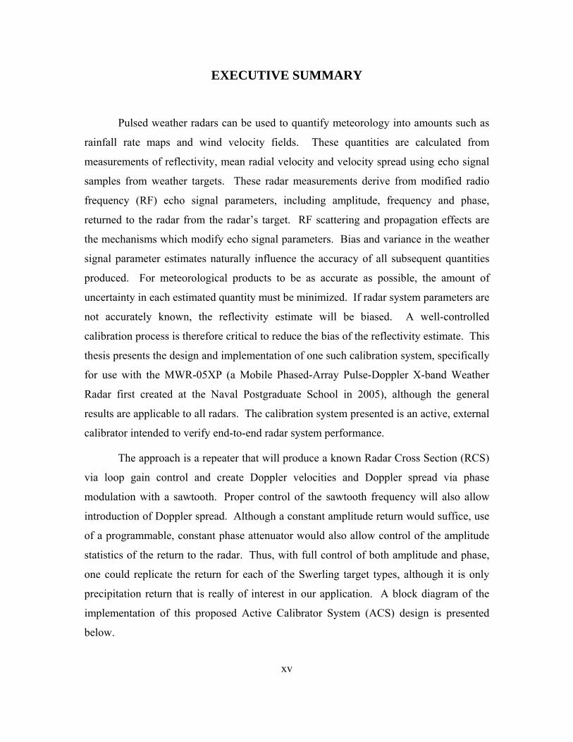
The approach is a repeater that will produce a known Radar Cross Section (RCS)
via loop gain control and create Doppler velocities and Doppler spread via phase
modulation with a sawtooth. Proper control of the sawtooth frequency will also allow
introduction of Doppler spread. Although a constant amplitude return would suffice, use
of a programmable, constant phase attenuator would also allow control of the amplitude
statistics of the return to the radar. Thus, with full control of both amplitude and phase,
one could replicate the return for each of the Swerling target types, although it is only
precipitation return that is really of interest in our application. A block diagram of the
implementation of this proposed Active Calibrator System (ACS) design is presented
below.
xvi
The reflectivity for a weather radar contains radar system parameters which may
not be precisely known. The objective of calibration is to determine the composite of
these parameters. The composite of these factors is also known as the radar system
calibration constant. In Dr. Jeffrey Knorr’s paper, “Weather Radar Equation Correction
for Frequency Agile and Phased Array Radars,” it has been shown that, for the case
where the reference target is on boresight, θ = 0, the measurement is made at the
reference frequency, λ = λ0, and the range is short (La = 1) the radar system calibration
constant can be described as:
( )3 420
20
4 outt rx
s
R PPG GL
πλ σ
⎡ ⎤⎡ ⎤= ⎢ ⎥⎢ ⎥⎢ ⎥⎣ ⎦ ⎣ ⎦
From this equation, it is clear that a measurement of receiver output power and
range for a reference target of known cross-section (θ = 0, λ = λ0, La = 1) permits the
radar system constant on the left side to be determined and the radar calibrated for
reflectivity estimation. Phase modulation is required to produce Doppler shift, according
to:
( ) ( ) ( )cos Re c j tj tcv t A t t A e e θωω θ ⎡ ⎤= + =⎡ ⎤⎣ ⎦ ⎣ ⎦ .
For θ(t) periodic where the phase modulated signal has a spectrum given by a sawtooth
waveform of amplitude adjusted to produce a phase change that is a multiple of 2π (see
waveform pictured below) then,
( ) ( ) ( )Re where 2c mj f mf tv t A e mθ π+= Δ = .
xvii
The signal is translated (Doppler shifted) from frequency cf to frequency c mf mf+ .
By cycling through 360° (2π) of phase at this periodic rate a known
frequency/Doppler shift is produced against which the weather radar can be calibrated.
This periodic phase cycling (and thus frequency translation) is implemented in the ACS
using a digital phase shifter. Velocity spread can be added to the Doppler shifted signal
by varying the frequency of the sawtooth waveform used in the phase modulator. The
frequency should be varied in accordance with a Gaussian random variable that has been
low pass filtered to produce a signal with the desired correlation time.
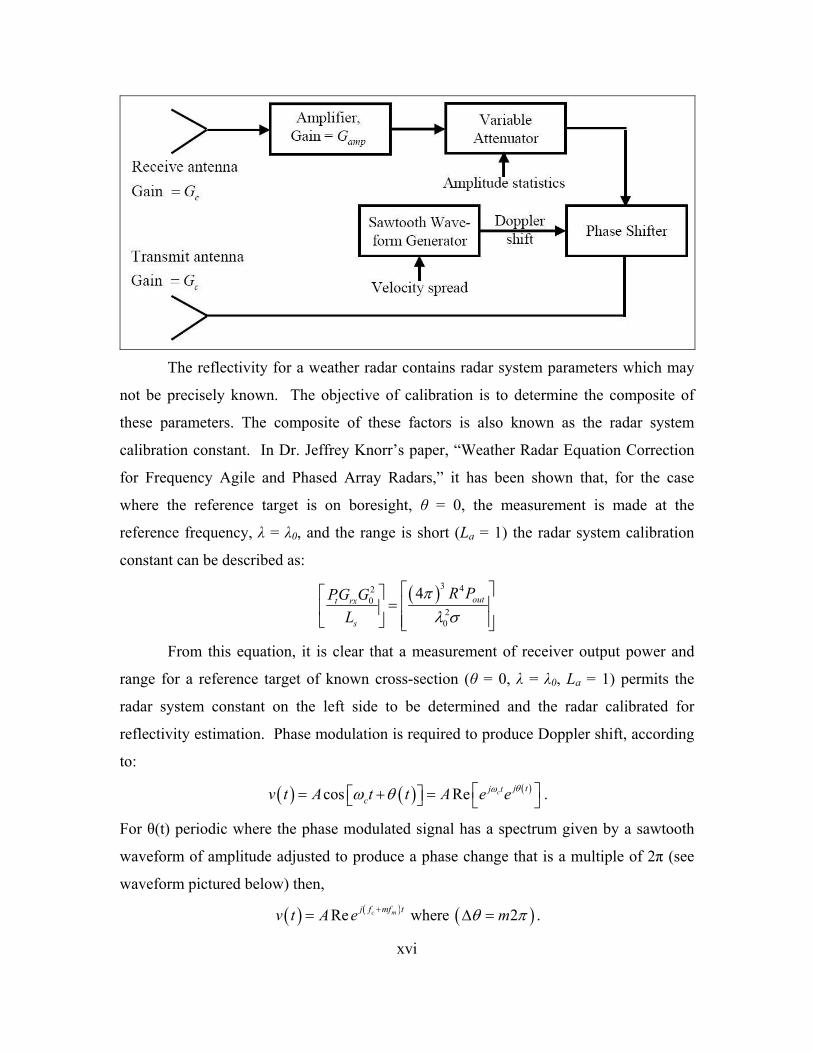
On the basis of these principles, the ACS was constructed (RF box internal
configuration digital photograph follows):
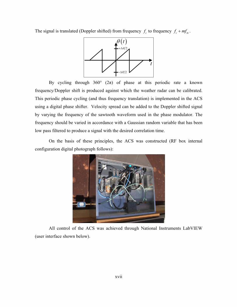
All control of the ACS was achieved through National Instruments LabVIEW
(user interface shown below).
xviii
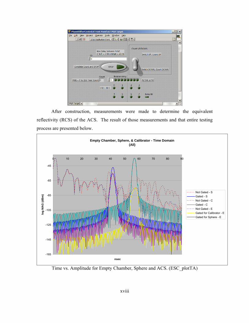
After construction, measurements were made to determine the equivalent
reflectivity (RCS) of the ACS. The result of those measurements and that entire testing
process are presented below.
Empty Chamber, Sphere, & Calibrator - Time Domain(All)
-165
-145
-125
-105
-85
-65
-45
0 10 20 30 40 50 60 70 80 90
nsec
log
MA
G (d
Bm
)
Not Gated - SGated - SNot Gated - CGated - CNot Gated - EGated for Calibrator - EGated for Sphere - E
Time vs. Amplitude for Empty Chamber, Sphere and ACS. (ESC_plotTA)
xix
Empty Chamber, Sphere, & Calibrator - Frequency Domain
-65
-60
-55
-50
-45
-40
-35
-30
-259 9.1 9.2 9.3 9.4 9.5 9.6 9.7 9.8 9.9 10
GHz
log
MA
G (d
Bm
)
Not Gated - SGated - SNot Gated - CGated - CNot Gated - EGated for Calibrator - EGated for Sphere - E
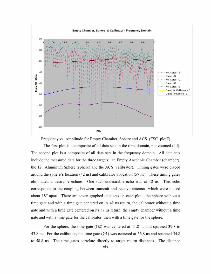
Frequency vs. Amplitude for Empty Chamber, Sphere and ACS. (ESC_plotF)
The first plot is a composite of all data sets in the time domain, not zoomed (all).
The second plot is a composite of all data sets in the frequency domain. All data sets
include the measured data for the three targets: an Empty Anechoic Chamber (chamber),
the 12” Aluminum Sphere (sphere) and the ACS (calibrator). Timing gates were placed
around the sphere’s location (42 ns) and calibrator’s location (57 ns). These timing gates
eliminated undesirable echoes. One such undesirable echo was at <2 ns. This echo
corresponds to the coupling between transmit and receive antennas which were placed
about 18” apart. There are seven graphed data sets on each plot: the sphere without a
time gate and with a time gate centered on its 42 ns return, the calibrator without a time
gate and with a time gate centered on its 57 ns return, the empty chamber without a time
gate and with a time gate for the calibrator, then with a time gate for the sphere.
For the sphere, the time gate (G2) was centered at 41.8 ns and spanned 39.8 to
43.8 ns. For the calibrator, the time gate (G1) was centered at 56.8 ns and spanned 54.8
to 58.8 ns. The time gates correlate directly to target return distances. The distance
xx
(range) from transmit and receive antennas in the anechoic chamber to the target pedestal
inside the chamber is 19 feet (or 38.6 ns in time). The distance is traversed twice (once to
the target and then from the target) at the speed of light. The reason the time gate for the
sphere was observed at and consequently set at 42 ns is the sphere was suspended from
the ceiling of the chamber above and slightly behind the target pedestal inside the
anechoic chamber. This added approximately an additional 1.6 feet of distance and 3 ns
of time because the hypotenuse rather than the longest leg of the triangle was traversed.
The reason the time gate for the calibrator was observed at and consequently set at 57 ns
is different than for the sphere. This time gate was approximately 8 ns greater because of
the time delay due to transmission line lengths rather than target distance. The 8 ns is
almost 8 feet (one-way path), slightly greater than the straight line distance between
transmit and receive antennas of the ACS (as expected). See the example calculations
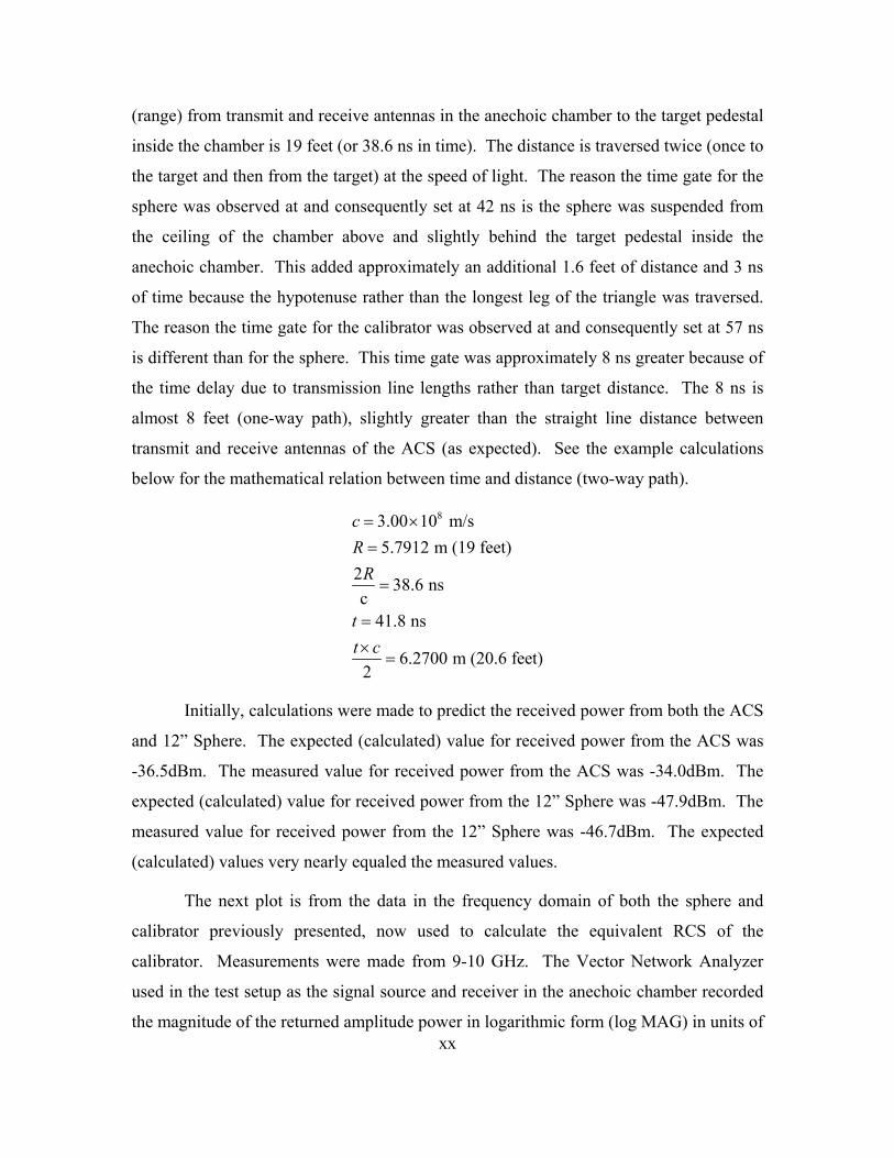
below for the mathematical relation between time and distance (two-way path).
83.00 10 m/s5.7912 m (19 feet)
2 38.6 nsc
41.8 ns
6.2700 m (20.6 feet)2
cR
R
tt c
= ×=
=
=×
=
Initially, calculations were made to predict the received power from both the ACS
and 12” Sphere. The expected (calculated) value for received power from the ACS was
-36.5dBm. The measured value for received power from the ACS was -34.0dBm. The
expected (calculated) value for received power from the 12” Sphere was -47.9dBm. The
measured value for received power from the 12” Sphere was -46.7dBm. The expected
(calculated) values very nearly equaled the measured values.
The next plot is from the data in the frequency domain of both the sphere and
calibrator previously presented, now used to calculate the equivalent RCS of the
calibrator. Measurements were made from 9-10 GHz. The Vector Network Analyzer
used in the test setup as the signal source and receiver in the anechoic chamber recorded
the magnitude of the returned amplitude power in logarithmic form (log MAG) in units of
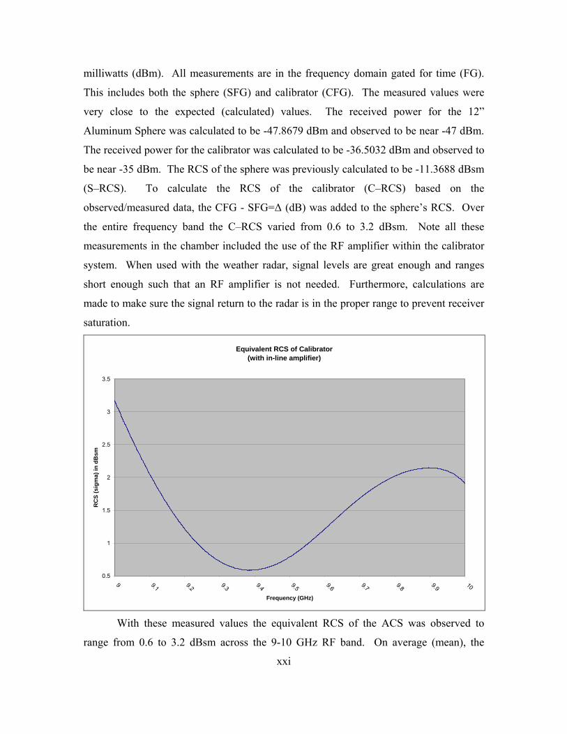
xxi
milliwatts (dBm). All measurements are in the frequency domain gated for time (FG).
This includes both the sphere (SFG) and calibrator (CFG). The measured values were
very close to the expected (calculated) values. The received power for the 12”
Aluminum Sphere was calculated to be -47.8679 dBm and observed to be near -47 dBm.
The received power for the calibrator was calculated to be -36.5032 dBm and observed to
be near -35 dBm. The RCS of the sphere was previously calculated to be -11.3688 dBsm
(S–RCS). To calculate the RCS of the calibrator (C–RCS) based on the
observed/measured data, the CFG - SFG=Δ (dB) was added to the sphere’s RCS. Over
the entire frequency band the C–RCS varied from 0.6 to 3.2 dBsm. Note all these
measurements in the chamber included the use of the RF amplifier within the calibrator
system. When used with the weather radar, signal levels are great enough and ranges
short enough such that an RF amplifier is not needed. Furthermore, calculations are
made to make sure the signal return to the radar is in the proper range to prevent receiver
saturation.
Equivalent RCS of Calibrator(with in-line amplifier)
0.5
1
1.5
2
2.5
3
3.5
9 9.1 9.2 9.3 9.4 9.5 9.6 9.7 9.8 9.9 10
Frequency (GHz)
RC
S (s
igm
a) in
dB
sm
With these measured values the equivalent RCS of the ACS was observed to
range from 0.6 to 3.2 dBsm across the 9-10 GHz RF band. On average (mean), the
xxii
equivalent RCS of the ACS was 1.4934 dBsm. The median was 1.5101 dBsm. The high
value was 3.1742 dBsm at 9 GHz and the low value was 0.5862 dBsm at 9.38 GHz.
An active calibrator system (ACS) for weather radar was successfully designed
and implemented. The ACS was verified to be a functional weather radar active
calibration system under laboratory testing. It successfully provided the means (met the
requirements) to verify all three of the signal parameters measured (estimated) by a
weather radar. These include the zeroth Doppler moment (reflectivity), first Doppler
moment (average radial velocity), and second Doppler moment (velocity spread).
xxiii
ACKNOWLEDGMENTS
I would like to thank the many people who were involved with the completion of
both my thesis and Masters Degrees at the Naval Post Graduate School (NPS). Without
the assistance of these people, I would not have been able to achieve so much or to get to
where I am today. First, I would like to thank Dr. Jeffrey Knorr who acted as my
principle advisor throughout the course of my thesis and my two years at NPS. I learned
a great deal from Dr. Knorr in and out of the classroom and consider myself fortunate to
have been a part of his research. I also credit Bob Broadston for a large part of the
success of my thesis. Bob continually shared his experience with me, and always made
me feel a part of a working relationship with him. I cannot thank Bob enough for his
constant assistance in addressing many of the day to day issues that arose as I completed
the research portion of my thesis. I would also like to thank Lt. Colonel Terry Smith. As
an active member of the United States Air Force and the Program Officer of the
Information Sciences Department, Lt. Col. Smith provided me with an insightful,
practical perspective that wholly complemented my meetings with Dr. Knorr. I would
like to thank him for the time he committed to advising me during my thesis research and
editing my written thesis. Finally, I would also like to acknowledge Dr. David Jenn, an
outstanding professor, for his instruction and guidance during my time at NPS.
At NPS, I was given the opportunity to learn at an institution that provides
practical skills critical to our nation’s defense, but also holds high the value of education
beyond mere training. I am extremely honored to have had the privilege to attend one of
our nations leading defense institutions while serving my country as a U.S. Federal
Government civilian employee. I trust that our nation’s leadership will continue to value
unique centers of excellence for defense matters, such as the Naval Postgraduate School,
and civilian defense programs, such as the one in which I participated.
To all of those individuals from whom I have learned during the course of my
formal education, thank you. Both professors and peers were critical to the success
achieved during my educational journey. To my family and friends, I will never forget

xxiv
what you have done for me along the way. While the completion of this thesis and these
graduate degrees marks the end of a chapter in my educational journey, I know it
certainly is not the end of my education. I look forward to furthering my education
while serving my country as I continue my career.
1
I. INTRODUCTION
A. BACKGROUND
Pulsed weather radars produce estimates of reflectivity, mean radial velocity and
velocity spread using echo signal samples from a wide variety of weather targets. From
these radar return signals, other meteorological quantities such as rainfall rate and wind
field characteristics are also derived. Estimates are derived from the parameters of the
modified radio frequency (RF) echo signal (amplitude and frequency/phase) scattered
from the target back in the direction of the radar. RF scattering and propagation effects
are the mechanisms which modify radar echo signal parameters and it is those
modifications that contain the desired weather-related information as a modulation of the
carrier wave. Bias and variance in the weather signal parameter estimates naturally
influence the accuracy of all subsequent quantities produced, and condition assessments
made. For meteorological products to reflect weather conditions as accurately as
possible, the uncertainty of each estimate must be minimized, or accurately characterized.
If radar system parameter accuracies are not precisely known, the reflectivity estimate
will be biased and thus, assessments of true conditions could be either misleading or
masked. A well-controlled calibration process is therefore critical to reduce reflectivity
bias due to imprecise knowledge of the radar system parameters. There may also be bias
associated with the statistical estimation process and its resulting estimator, but poor
calibration is the most serious source of error. The variance of the estimate of interest
will depend on the number of samples and their correlation.
B. RESEARCH OBJECTIVE
The research objective of this thesis is to design and implement a radar calibration
system (calibrator). The calibrator is for specific use with the Naval Postgraduate
School’s MWR-05XP1 X-band weather radar, but the general concept is applicable to all
1 World’s first and currently (2007) only Mobile Weather Radar created in 2005 operating at X-band
in Pulse-Doppler with a Phased-Array. In acronym, this is the MWR-05XP.
2
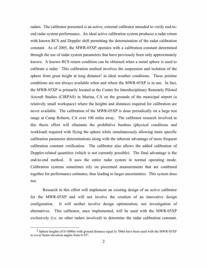
radars. The calibrator presented is an active, external calibrator intended to verify end-to-
end radar system performance. An ideal active calibration system produces a radar return
with known RCS and Doppler shift permitting the determination of the radar calibration
constant. As of 2005, the MWR-05XP operates with a calibration constant determined
through the use of radar system parameters that have previously been only approximately
known. A known RCS return condition can be obtained when a metal sphere is used to
calibrate a radar. This calibration method involves the suspension and isolation of the
sphere from great height at long distance2 in ideal weather conditions. These pristine
conditions are not always available when and where the MWR-05XP is in use. In fact,
the MWR-05XP is primarily located at the Center for Interdisciplinary Remotely Piloted
Aircraft Studies (CIRPAS) in Marina, CA on the grounds of the municipal airport (a
relatively small workspace) where the heights and distances required for calibration are
never available. The calibration of the MWR-05XP is done periodically on a large test
range at Camp Roberts, CA over 100 miles away. The calibrator research involved in
this thesis effort will eliminate the prohibitive burdens (physical conditions and
workload) required with flying the sphere while simultaneously allowing more specific
calibration parameter determinations along with the inherent advantage of more frequent
calibration constant verification. The calibrator also allows the added calibration of
Doppler-related quantities (which is not currently possible). The final advantage is the
end-to-end method. It uses the entire radar system in normal operating mode.
Calibration systems sometimes rely on piecemeal measurements that are combined
together for performance estimates, thus leading to larger uncertainties. This system does
not.
Research in this effort will implement an existing design of an active calibrator
for the MWR-05XP and will not involve the creation of an innovative design
configuration. It will neither involve design optimization, nor investigation of
alternatives. This calibrator, once implemented, will be used with the MWR-05XP
exclusively (i.e. no other radars involved) to determine the radar calibration constant.
2 Sphere heights of 0-1000m with ground distance equal to 700m have been used with the MWR-05XP
to cover beam elevation angles from 0-55°.
3
The type of signal used by the calibrator in this process will be of the minimum required
complexity, although the performance parameters involved are those that most accurately
reflect operational weather characteristics.
The primary hardware involved with this thesis effort will be a digital phase
shifter, programmable attenuator, and real-time controller with reconfigurable chassis.
The only software involved will be LabVIEW (in the manipulation of the controller
hardware) and MATLAB (in the analysis of data and display of results).
C. RELATED WORK
The thesis by Schroder presents a weather radar signal simulator. According to
the abstract of the Schroder thesis,
the simulator was developed in MATLAB and implemented several different functionalities allowing for stepped frequency, multiple pulse repetition frequencies (PRFs), pulse compression using a chirp waveform, and variation of both weather and radar input parameters. Post-detection processing capabilities include autocorrelation and Fast Fourier Transform (FFT - for single PRF only); estimation of weather parameters such as reflectivity (Z); average Doppler, radial velocity, and velocity spread; pedagogical plots including a phasor plot of phase change over time and a velocity histogram, instantaneous observed reflectivity and power for each pulse over time.[1]
The output of Schroder’s simulator was modified to provide the calibrator controller
software with Doppler frequencies and amplitude levels indicative of real-world weather
effects for use in the calibration process.
The article by Marshall and Hitschfeld investigates the random fluctuations of the
radar echo produced from a random array of scatterers (such as weather scatterers).
According to the introduction to this article, “the intent is to establish (theoretically and
by analogue computation) the extent of the limitation these fluctuations have on the
accuracy of the measurement information obtainable. Additionally, what improvements
may be effected by averaging or by modifying the method of pulsing or scanning are
4
explored.”[2] The Marshall and Hitschfeld theory is used in this research to produce the
amplitude levels indicative of real-world weather effects for use in the calibration
process.
The report by Pratte and Ice explores external radar calibration methods.
According to the executive summary of the Pratte and Ice report, “the targeted radar for
this report is the WSR-88D, the weather radar in use (as of 2007) by the U.S. National
Weather Service in its national weather radar network. It reviews availability and
feasibility of “calibration aids”, equipment and software that will assist in verifying
WSR-88D reflectivity measurement and in reducing its uncertainty.”[3] The
recommendations of the Pratte and Ice report were used to enhance understanding of the
general weather radar calibration problem and its alternative solutions.
The text by Doviak and Zrinc emphasizes the application of Doppler radar for the
observations of stormy and clear air. According to the introduction (1.2) to the text, “it
presents a comprehensive treatment of the techniques used in extracting meteorological
information from weather echoes and relates radar and signal characteristics to
meteorological patterns.”[4] The Doviak and Zrinc text served as a classic reference
book on radar theory and accepted techniques applied to meteorology.
The paper by Knorr presents a derivation of two correction factors to the classic
Probert-Jones weather radar equation for use with frequency agile, phased array weather
radars. According to the abstract of this paper, “the result is an extended weather radar
equation for use with these advanced weather radars. The two derived factors account for
the effect of a changing RF carrier and electronic beaming steering not present in classic
weather radars when computing a reflectivity estimate from weather signal data
samples.”[5] The Knorr paper, as well as personal discussions with its author (an advisor
to this thesis), provided the necessary understanding of the unique calibration
requirements of these advanced weather radars from theory to practical application.
Chapter Four of the Federal Meteorological Handbook discusses potential
operational uses of the WSR-88D products as well as the structure of certain
meteorological phenomena. According to the introduction to Chapter 4 (4.1), “it
5
provides information on observing and forecasting meteorological phenomena using this
radar’s products.”[6] Of particular interest in the development of this thesis’s research
was the discussion in early sections of operationally troublesome radar returns due to
such things as ground clutter and sidelobes. The pictorial representations in the
Meteorological Handbook were invaluable.
D. ORGANIZATION OF THE THESIS
There are four main chapters and several appendices which comprise this thesis.
Chapter I gives a background of the radar calibration problem along with the research
objectives for this specific project. Related works are introduced and discussed. An
executive summary is also included. Chapter II explains the theory behind the operation
of weather radar (how the three principle quantities of reflectivity, velocity and velocity
spread are measured and related to signal parameters). The density function for
precipitation, relation between signal correlation and velocity spread, and fundamentals
of weather radar signal parameter estimation are given. Chapter III describes the specific
calibrator design in explicit detail. Measured results are presented and explained in
appendices. Chapter IV draws conclusions on the success of the implementation and
provides recommendations for future work.

6
THIS PAGE INTENTIONALLY LEFT BLANK
7
II. BACKGROUND AND SUPPORTING THEORY
This chapter presents and explains the theory behind the operation of weather
radar. The discussion includes how the three principle quantities of reflectivity3, mean
radial velocity4 and velocity spread5 are measured and are related to radar signal
parameters. The density function for precipitation, relation between signal correlation
and velocity spread, and fundamentals of weather radar signal parameter estimation are
given.
Significant portions have been excerpted from Chapter 2 “Weather Radar and
Weather/Rain Theory” of Ulf Schroder’s thesis “Development of a Weather Radar Signal
Simulator to Examine Sampling Rates and Scanning Schemes.” Both Schroder’s thesis
and this thesis are in support of the larger research project/interest of Dr. Jeffrey Knorr
(advisor to both theses). Much of the background and supporting theory used in
Schroder’s thesis (completed 2005) applies to this thesis (completed 2008) and the larger
research project/thrust.
A. WEATHER RADAR VS. TRADITIONAL RADAR
Weather radar samples the scattered RF energy from distributed targets such as
precipitation, hail, snow, melting ice, and clear air. This is unlike traditional radar which
views these returns as clutter, unwanted echoes that interfere with the observation of the
return from a point target of interest. Traditional radar usually implements Doppler
filtering to discriminate between slow moving weather clutter and fast moving point
targets. In this application, the scattered energy contains descriptive characteristics of the
weather condition.
3 Function of the scatterer intensity. 4 Function of the mean component of scatterer motion in the radial direction from the radar. 5 Function of the variability of Doppler velocity values due to turbulence within and velocity shear
across the sampling volume.
8
B. RADAR RESOLUTION CELL
Weather radar differs from traditional radar in another important way. Traditional
radar seeks to encapsulate its target of interest (approximately a point target) entirely
within a single radar resolution cell. For weather radar this is neither practical nor
informative at either the micro or macro scales. It is impractical to image a single rain
drop or an entire storm and even if it were possible the information provided would not
be especially useful. Instead, weather radars image a volumetric segment of the
meteorological phenomena of interest. This volume is defined by a segment of
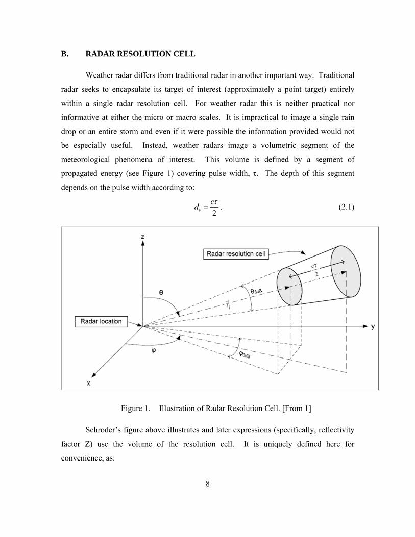
propagated energy (see Figure 1) covering pulse width, τ. The depth of this segment
depends on the pulse width according to:
2vcd τ
= . (2.1)
Figure 1. Illustration of Radar Resolution Cell. [From 1]
Schroder’s figure above illustrates and later expressions (specifically, reflectivity
factor Z) use the volume of the resolution cell. It is uniquely defined here for
convenience, as:
9
( )( ) ( )1
4 2 2ln 2c B BcV V R Rπ τθ φ ⎛ ⎞Δ = = ⎜ ⎟
⎝ ⎠ (2.2)
See Chapter II, Section E, Subsection 1, “Antenna Gain and Beam effective Solid
Angle,” for an explanation of the last factor, ( )
12ln 2
.
C. SWERLING TARGET TYPES
Meteorological conditions produce a radar target return that varies with time.
Besides the target itself, fluctuations in the target’s return may also be caused by
variations in the medium between the target and the radar (atmospheric and
meteorological conditions not the intended target), radar system instabilities (platform
motion and equipment instabilities), target aspect changes, and many other variables. In
order to analyze all of this variation, the target is modeled as an overall system. For
systems analysis purposes, only the ‘gross’ behavior of a target needs to be known, not
every detail of all the complicated physics involved in the complex scattering situation.
Therefore, fluctuations caused by all of these many sources (exclusive of those caused
simply by a change in range) are usually grouped together and represented by a single
quantity for a specific target type.
The following excerpt was relayed from the radar text by Skolnik, although nearly
every radar text contains some explanation of Swerling target types. Let σ be a random
variable with a probability density function (PDF) that depends on the factors associated
with target fluctuations other than a change in range and the overbar represents the
average value of the random variable. Two PDFs are commonly used:
1( ) , PDF #1p e σ σσσ
−= (2.3)
and
22
4( ) , PDF #2p e σ σσσσ
−= (2.4)
These two PDFs approximate the nature of the scattering of RF energy from many
targets. There are targets which consist of many independent scattering elements of
10
which no single one (or few) dominates (PDF #1) and targets which have one main
scattering element that dominates in the presence of smaller independent scattering
sources (PDF #2). These two PDFs along with the rate at which the fluctuations take
place allow the definition of four types of radar targets, also known as Swerling target
types. Swerling target types I and II are associated with PDF #1 and types III and IV
with PDF #2. The rate of the fluctuations in this scattering is the other differentiating
factor which further defines the Swerling target type. There are targets with slow
fluctuations (scan-to-scan) and targets with rapid fluctuations (pulse-to-pulse). Swerling
target types I and III are of the former and types II and IV of the latter.
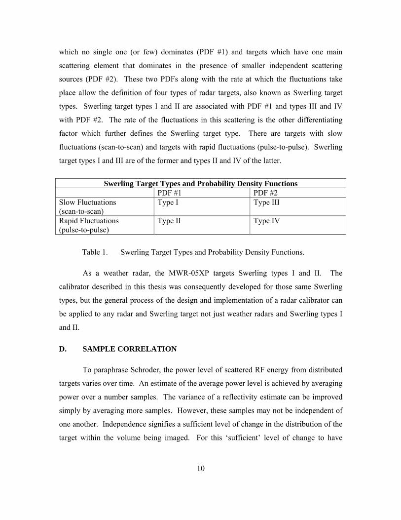
Swerling Target Types and Probability Density Functions
PDF #1 PDF #2 Slow Fluctuations (scan-to-scan)
Type I Type III
Rapid Fluctuations (pulse-to-pulse)
Type II Type IV
Table 1. Swerling Target Types and Probability Density Functions.
As a weather radar, the MWR-05XP targets Swerling types I and II. The
calibrator described in this thesis was consequently developed for those same Swerling
types, but the general process of the design and implementation of a radar calibrator can
be applied to any radar and Swerling target not just weather radars and Swerling types I
and II.
D. SAMPLE CORRELATION
To paraphrase Schroder, the power level of scattered RF energy from distributed
targets varies over time. An estimate of the average power level is achieved by averaging
power over a number samples. The variance of a reflectivity estimate can be improved
simply by averaging more samples. However, these samples may not be independent of
one another. Independence signifies a sufficient level of change in the distribution of the
target within the volume being imaged. For this ‘sufficient’ level of change to have
11
occurred there exists a minimum required period of time. This minimum time period
guarantees samples are not correlated from one observation period to the next.
Schroder explains, “The power spectral density of a meteorological signal is
approximately Gaussian and can be written as
( )222
0( )f
f f
S f S eσ
⎧ ⎫−⎪ ⎪−⎨ ⎬⎪ ⎪⎩ ⎭= (2.5)
where f is the Doppler frequency and 2fσ is the Doppler spectrum variance. Taking the
Fourier transform of Equation (2.5) and normalizing results in the correlation coefficient
( )2
22t e τ
τσρ
⎛ ⎞−⎜ ⎟⎜ ⎟⎝ ⎠ (2.6)
where 2τσ is the time spectrum variance and is related to 2
fσ by
12 f
τσ πσ= (2.7)
and
2 vf
σσλ
= . (2.8)
By using the correlation coefficient a measure of minimum difference in time can
be estimated ensuring dependent or independent samples. Nathanson claims that for
independent sampling ( ) 0.02ρ τ < is required whereas ( ) 0.15ρ τ > will ensure
dependence. Doviak and Zrnić set a correlation threshold for coherence at ( )2 1eρ τ −≥
which corresponds to a value of ( ) 0.6ρ τ ≥ . Using this threshold renders
0.25Sv
T λπσ
≤ (2.9)
For highly correlated samples."
A level of ‘sufficient’ change has occurred within an observation period for a
sample so that any subsequent samples may be deemed independent if:
0.70sv
T λπσ
> (2.10)
12
where sT is the sample time period and vσ is the RMS velocity spread.
E. ESTIMATION OF POWER DENSITY AND REFLECTIVITY (Z)
1. Antenna Gain and Beam effective Solid Angle
Antenna gain varies depending on azimuth and elevation angles for directive
antennas. For a point target, antenna gain is constant only for a fixed azimuth and
elevation angle defined between the radar and a point in space at a specific time. For a
volumetric target, antenna gain varies across a range of azimuth and elevation angles
defined between the radar and a volume of space at a specific time. The antenna pattern
function, ( ),f θ φ , integrated over the solid angle corresponding to the radar resolution
cell is used to estimate a value of antenna gain for volumetric targets.
From Schroder (and Probert-Jones as the original source), “The magnitude of the
antenna pattern function is first squared to yield a power relation and squared again to
agree with the two way propagation of radar.
( ) 4
4
,f dπ
θ φ Ω∫ (2.11)
The Gaussian Pattern Model is the antenna pattern function that will be used. It
provides a good approximation of the main beam between the half power points.
Extending it in both azimuth and elevation provides
( )2 2
2 221 1
1 1, , , 2 2
f eθ φγ δθ φ θ θ φ φ⎡ ⎤
− +⎢ ⎥⎢ ⎥⎣ ⎦= ≤ ≤ (2.12)
where 2
2 1
4 ln 2θγ = and
22 1
4 ln 2φδ = , and 1 1, θ φ are the half power beam widths in the
orthogonal planes.
Performing integration over the solid angle gives
( ) ( )2 2
2 22 2
4 1 1
4
, 18ln 2
f d e d dθ φγ δ
π
πθ φθ φ θ φ ξ⎡ ⎤+∞ +∞ − +⎢ ⎥⎢ ⎥⎣ ⎦
−∞ −∞
Ω = = −∫ ∫ ∫ (2.13)
13
where 0.034ξ < and represents the contributions from the sidelobes. In a further
approximation, at its maximum value the ( )1 ξ− term contributes a negligible 0.15 dB
and therefore can be ignored.”
The final form of the expression used to approximate beam solid angle for
volumetric targets is
( )4 1 1
4
,8ln 2
f dπ
πθ φθ φ Ω =∫ . (2.14)
See also the Probert-Jones paper[7]. The equation above gives beam solid angle
contributing to the volume return. Note this result is based on a Gaussian approximation
to the beam pattern. As Dr. Knorr shows in his paper, integration of an actual antenna
pattern will generally result in a correction which may not be negligible.
2. Physics of Precipitation
The following presents some basics in precipitation physics relevant to
developing a physical understanding of precipitation, specifically rain the primary target
of weather radar. The following three sections have been selectively chosen from a
larger discussion of the physics of precipitation by Schroder. Each of the three sections’
text has been paraphrased and equations reproduced verbatim.
a. Size and Shape
Raindrop size determines the terminal velocity at which the drop falls and
the shape of the drop. Small drops, with a diameter D < 0.35 mm, are spherical. Medium
size drops, with diameters 0.35 mm < D < 4 mm, have progressively flattened bases and
are approximated as spheroids. Large drops, D > 4 mm, do not last very long and tend to
break apart upon collision. The largest drops, D > 10 mm, are unstable and break apart
without collision.
14
b. Drop Size Distribution (DSD)
Radar cross section (RCS) density, η , is the average RCS density per unit
volume, as previously mentioned, and for independent scattering is the sum of the RCS of
all scatters in the return volume divided by that volume. The DSD represents the
diameter density (mm/m3) of drops for all diameters. The Marshall-Palmer DSD
provides a general model:
( ) 0
0.21 1
3 3 10
4.1 mm8 10 m mm
DN D N e
RN
−Λ
− −
− −
=
Λ =
= ×
(2.15)
Applying truncation with a maximum drop diameter of maxD yields
( ) 0 max
max
, 0,
DN e D DN D
D D
−Λ⎧ <⎪= ⎨<⎪⎩
. (2.16)
c. Rainfall Rate
Rainfall rate determines the depth of accumulated water per unit time. It
can be derived from water content and fall speeds. A cloud’s water density is
( )3
06 wM D N D dDπ ρ∞
= ∫ (2.17)
where wρ is the water density of a rain drop.
Turning this into rainfall rate
( ) ( )3
06R D N D v D dDπ ∞
= ∫ . (2.18)
Rainfall rate is estimated from reflectivity using any one of a number of
slightly different models, Z = Arb. Z = 300r1.4, for example, is the current WSR-88D
default model. The best rainfall model depends upon the type of storm or equivalently,
drop size distribution. Dual polarization radars provide more information about drop size
and thus rainfall rate. Latest results from JPOL experiment (dual polarization WSR-88D
at NSSL) are given in Ryzhkov[8].
15
3. Weather Radar Range Equation and Estimation of Reflectivity
Again, following Schroder, the basic form of the radar range equation (neglecting
minor losses):
( )
2
3 44t t r
rPG GP
Rσλ
π= (2.19)
“In the basic form of the weather radar equation radar cross section (RCS), σ, is
replaced by RCS density, η , which is the expected RCS density per unit volume. Since
the target is a volume target, the expected return needs to be integrated over the whole
volume, which can be divided into the solid angle and depth of the return. Letting the
power level at the target be
24 4t t t t
targetPG PGP dA d
Rπ π= = Ω (2.20)
and integrating the return power over the return volume renders
( )
( )2 22 4
1 13 2 2 2,
1024 ln 24
cR
t t r t t rr r
R
PG G PG GdR cP dP f dR R
τ
λ λ θ φτη θ φ ηππ
+
Ω
= = Ω =∫ ∫ ∫ (2.21)
recognizing that 2cR τ? .
Radar meteorologists use the reflectivity factor, Z, instead of RCS density where
5
24 wK Zπη
λ= (2.22)
and
61i
i VZ D
V ∈
≡ ∑ . (2.23)
Substituting Equation (2.22) into Equation (2.21) and solving for Z yields the reflectivity
estimator
µ2 2 4 2 2
2 22 5 31 1 1 1
1024 ln 2 1024 ln 2r r
t t r w t t r w
R RZ P PPG G c K PG G c K
π λ λλ τθ φ π τθ φ π
= = . (2.24)
16
For an assumed continuous distribution of drops sizes with diameter density
( )N D Equation (2.23) becomes
( )max
6
0
D
Z D N D dD= ∫ . (2.25)
Solving the integral form for an assumed Marshall-Palmer Drop Size Distribution
(DSD) Equation (2.15), yields
( )( )
6 070.21
0
6!
4.1
NZ D N D dDR
∞
−= =∫ (2.26)
Drops do not exist in sizes ranging up to infinite diameter, but are likely to be
limited by a maximum diameter. Doviak and Zrnić state that Equation (2.26)
overestimates Z and suggest a truncated DSD with maxD D= . In this case,
( )
( )070.21
7,4.1
NZ aR
γ−
= (2.27)
where maxa D= Λ and ( )7, aγ is the incomplete Gamma function. Equations (2.26) and
(2.27) provide an analytical means for computing Z.”
F. RADAR PRINCIPLES AND WEATHER RADAR EQUATION CORRECTION
The basic results for phased array weather radar are presented from Knorr’s
paper. This paper addresses issues unique to frequency hopping, phased array weather
radars and quantifies the need for a target of known radar cross section (RCS).
“The first term in the equation below indicates those radar system parameters
which may not be precisely known.
( ) ( )
( )
4 2 2200
3 4
cos
4t rx
outs a
PG G PL R L
λ λ θ λ σ
π
⎡ ⎤⎡ ⎤⎢ ⎥ =⎢ ⎥⎢ ⎥⎣ ⎦ ⎣ ⎦
(2.28)
where
λ0 = reference6 wavelength (m)
6 The choice of reference wavelength within the operating band of the radar is arbitrary.
17
Ls = radar system losses (ratio) La = atmospheric propagation loss (ratio)
outP = output power (W) R = range to target (m) Pt = transmit power Grx = receiver gain G0 = gain at the reference frequency, f0 λ = operating wavelength (m) θ = angle of the antenna beam with respect to boresight or the normal to the array face σ = target radar cross section (RCS) (m2)
The objective of calibration is to determine the composite of these factors with a
single measurement. To simplify this process, several conditions can be selected. These
include: calibration on boresight with the antennas of the active calibrator system (ACS)
and the radar (θ = 0), calibration at the reference RF center frequency (λ = λ0), and
calibration at a range that is short enough that atmospheric losses can be ignored (La = 1).
Then, the equation simplifies and rearranges to:
( )3 420
20
4 outt rx
s
R PPG GL
πλ σ
⎡ ⎤⎡ ⎤= ⎢ ⎥⎢ ⎥⎢ ⎥⎣ ⎦ ⎣ ⎦
(2.29)
With this relationship, a measure of the radar receiver’s output power and range
for a reference target of known cross-section (the ACS’s equivalent reflectivity) will
determine the radar system constant (left hand side of the equation).”
For frequency agile, phased array weather radars, the equation for reflectivity
takes the form
( ) ( ) ( )
( )4
202 423 2
00 0 00
1024ln 2 1cos
s a outbr br
t rxB B
L L PZ RPG G f fc K
λθ ϕ θπ τ λ
⎡ ⎤⎡ ⎤ ⎡ ⎤⎡ ⎤⎢ ⎥= ⎢ ⎥ ⎢ ⎥⎢ ⎥⎢ ⎥⎢ ⎥ ⎢ ⎥⎣ ⎦ ⎣ ⎦⎣ ⎦ ⎣ ⎦
(2.30)
where
Z = reflectivity (mm6/m3) λ0 = reference wavelength (m) Ls = radar system losses (ratio) La = atmospheric propagation loss (ratio) Pout = average output power (W)
R = range to target (m) c = speed of light in a vacuum = 3 x 10⁸ m/s τ = pulsewidth (s)
18
( ) ( ) 22 1 2 0.93 (H O)2K r rε ε= − + ≈
εr = hydrometeor relative permittivity
0brBθ and 0
brBϕ are the broadside 3 dB principal plane beamwidths at the reference
frequency
Pt = transmit power Grx = receiver gain G0 = gain at the reference frequency, f0 f = operating frequency (Hz) f0 = reference7 frequency (Hz) θ = angle of the antenna beam with respect to boresight or the normal to the array face
Note that the units of Z are given correctly (mm6/m3) by the first two terms of
Equation (2.30) if range is in millimeters, 0λ in the numerator of the first term is in
millimeters and the quantities in the denominator of the first term are in meters.
This is the corrected form of the classical Probert-Jones classical weather radar
equation as derived by Dr. Jeffrey Knorr in his paper, “Weather Radar Equation
Correction for Frequency Agile and Phased Array Radars.”
The third term contains radar system parameters which may not be precisely
known. The objective of calibration is to determine the composite effect of these factors.
The composite of these factors is also known as the radar system calibration constant. In
Dr. Knorr’s paper it has been shown that, for the case where the reference target is on
boresight, θ = 0, the measurement is made at the reference frequency, λ = λ0, and the
range is short (La = 1)
( )3 420
20
4 outt rx
s
R PPG GL
πλ σ
⎡ ⎤⎡ ⎤= ⎢ ⎥⎢ ⎥⎢ ⎥⎣ ⎦ ⎣ ⎦
. (2.31)
From Equation (2.31), it is clear that a measurement of receiver output power and
range for a reference target of known cross-section (θ = 0, λ = λ0, La = 1) permits the
radar system constant on the left side to be determined and the radar calibrated for
reflectivity estimation.
7 The choice of reference frequency within the operating band of the radar is arbitrary.
19
G. ESTIMATION OF VELOCITY
According to Schroder, “Pulsed radar can, by measuring the phase change
between consecutive pulses, estimate radial velocity. The effect, called Doppler, is the
frequency change that occurs due to the relative movement of a target with respect to the
radar. Considering a two-way propagation path renders a total phase change of
22 Rφ πλ
= (2.32)
In terms of angular frequency the result is
44 2rd
vd dR fdt dt
πφ πϖ πλ λ
= = = = (2.33)
where rv is the radial velocity and df is the Doppler frequency.
From a pulse pair, using a coherent detector, the phase change can be extracted
using
{ }
( )
{ }1*
1 1
*1 1
arg
arg
n
n n
jn n n n
n n
jn n n n
n n n n
V I jQ A eV
V V A A e
V V
φ
φ φ
φ
φ φ δφ
+ −+ +
+ +
= + =
=
=
= − =
(2.34)
leading to the single pulse pair velocity estimate
{ } { }* *1 1ˆ arg arg
4 4 4p
r n n n nP
fv V V V V
t Tλλδφ λ
πδ π π+ += = = (2.35)
where pT is time between pulses and pf is pulse repetition frequency.”
Also from Schroder, coherence between pulse pairs is required to measure phase
change over time for a volumetric target to minimize phase change from effects other
than radial movement. The variance of a velocity estimate can be improved simply by
averaging more samples. Building on the single pulse pair velocity estimate Equation
(2.35), the multiple pulse pair estimator becomes:
{ }1 1
*1 1
1 1
1 1 arg1 1 4
N Np
n n nn n
fv v V V
N Nλπ
− −
+ += =
= =− −∑ ∑$ . (2.36)
20
H. ESTIMATION OF VELOCITY SPREAD
Turbulence, wind shear, and differences in fall speed due to drop size are but a
few of the many directly influencing factors on the spread in radial velocity of
precipitation. There are even indirect factors (motion of the radar antenna) which impart
an apparent spread in velocity. The net effect of these factors is the width of the spread
in the velocity spectrum and the time for de-correlation between samples.
Schroder explains, “An estimate of the velocity spread can be computed using the
velocity samples obtained from a pulse pair comparison between single pulse pair
velocity estimates Equation (2.35). The estimator for sample variance is given by
µµ( )2
21
N
ii
v
v v
Nσ =
−=∑ $
(2.37)
and the estimator for standard deviation is”
µ µ2v vσ σ= . (2.38)
I. CALIBRATION REQUIREMENTS
Factors exist both internally (hardware and software) and externally
(environmental and remote sensing effects) that influence a radar’s measurements apart
from the target return that is trying to be quantified. The calibration process is used to
reduce the influence of these factors on the composite measurement. Internal calibrators
minimize system variations by separating the instrument from variable external
influences (such as through the use of known reference signals generated internally to test
internalized system components). External calibrators, however, operate completely
outside (and independent of) the instrument under test. By operating completely outside,
external calibrators incorporate those elements in the calibration process that describes
external influences that would effect the instrument’s measurements, but are not
considered with an internal calibration method. By operating independently, external
calibrators are able to calibrate for the same factors targeted by internal calibrators
without the calibrator being influenced in its calibration by the instrument under test.
With these two additional traits, external calibrators can verify whole-system calibration.
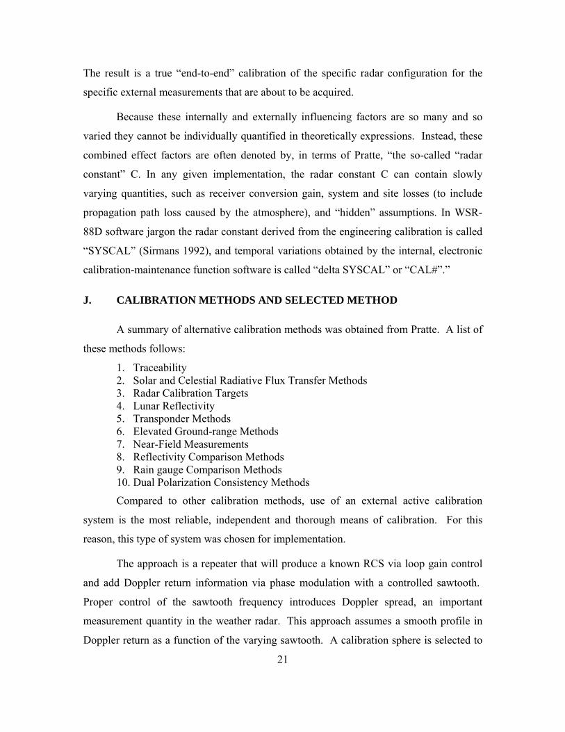
21
The result is a true “end-to-end” calibration of the specific radar configuration for the
specific external measurements that are about to be acquired.
Because these internally and externally influencing factors are so many and so
varied they cannot be individually quantified in theoretically expressions. Instead, these
combined effect factors are often denoted by, in terms of Pratte, “the so-called “radar
constant” C. In any given implementation, the radar constant C can contain slowly
varying quantities, such as receiver conversion gain, system and site losses (to include
propagation path loss caused by the atmosphere), and “hidden” assumptions. In WSR-
88D software jargon the radar constant derived from the engineering calibration is called
“SYSCAL” (Sirmans 1992), and temporal variations obtained by the internal, electronic
calibration-maintenance function software is called “delta SYSCAL” or “CAL#”.”
J. CALIBRATION METHODS AND SELECTED METHOD
A summary of alternative calibration methods was obtained from Pratte. A list of
these methods follows:
1. Traceability 2. Solar and Celestial Radiative Flux Transfer Methods 3. Radar Calibration Targets 4. Lunar Reflectivity 5. Transponder Methods 6. Elevated Ground-range Methods 7. Near-Field Measurements 8. Reflectivity Comparison Methods 9. Rain gauge Comparison Methods 10. Dual Polarization Consistency Methods
Compared to other calibration methods, use of an external active calibration
system is the most reliable, independent and thorough means of calibration. For this
reason, this type of system was chosen for implementation.
The approach is a repeater that will produce a known RCS via loop gain control
and add Doppler return information via phase modulation with a controlled sawtooth.
Proper control of the sawtooth frequency introduces Doppler spread, an important
measurement quantity in the weather radar. This approach assumes a smooth profile in
Doppler return as a function of the varying sawtooth. A calibration sphere is selected to
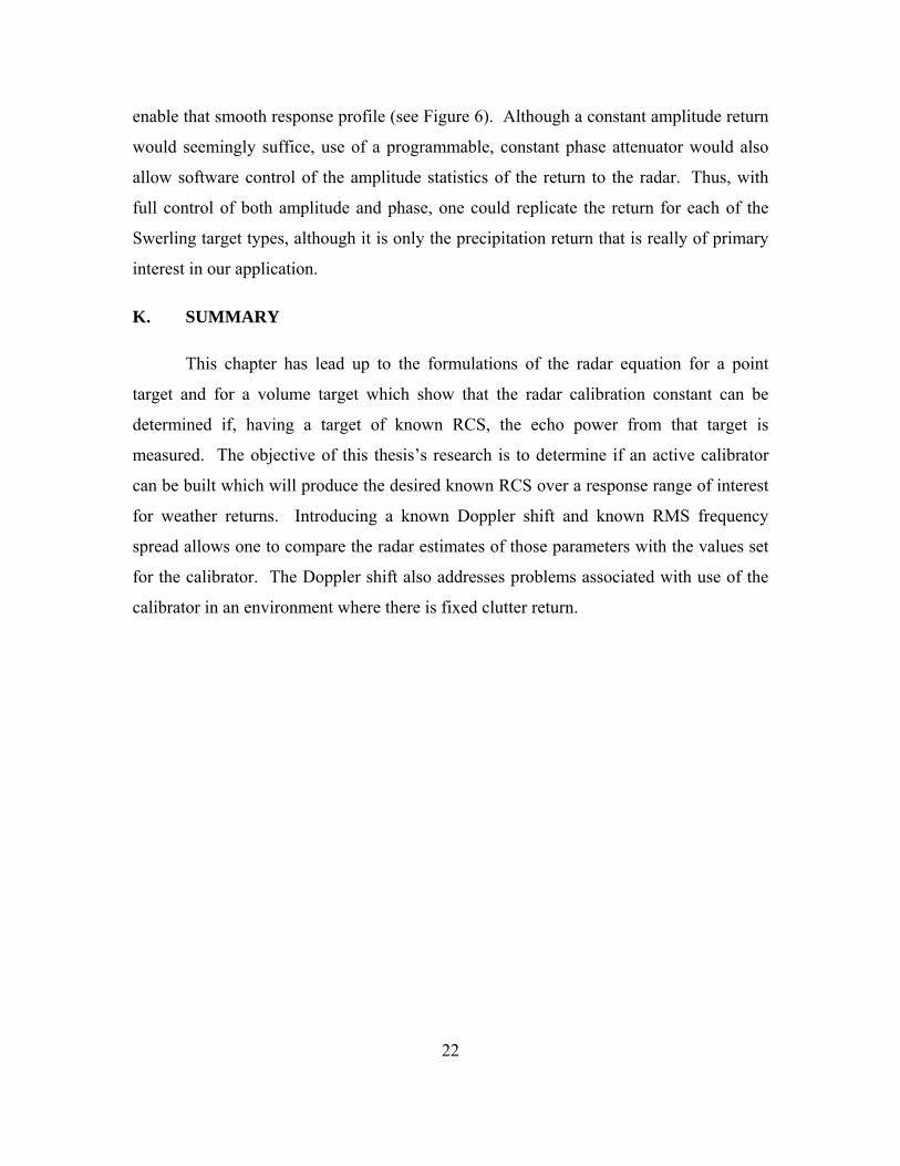
22
enable that smooth response profile (see Figure 6). Although a constant amplitude return
would seemingly suffice, use of a programmable, constant phase attenuator would also
allow software control of the amplitude statistics of the return to the radar. Thus, with
full control of both amplitude and phase, one could replicate the return for each of the
Swerling target types, although it is only the precipitation return that is really of primary
interest in our application.
K. SUMMARY
This chapter has lead up to the formulations of the radar equation for a point
target and for a volume target which show that the radar calibration constant can be
determined if, having a target of known RCS, the echo power from that target is
measured. The objective of this thesis’s research is to determine if an active calibrator
can be built which will produce the desired known RCS over a response range of interest
for weather returns. Introducing a known Doppler shift and known RMS frequency
spread allows one to compare the radar estimates of those parameters with the values set
for the calibrator. The Doppler shift also addresses problems associated with use of the
calibrator in an environment where there is fixed clutter return.
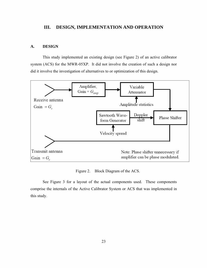
23
III. DESIGN, IMPLEMENTATION AND OPERATION
A. DESIGN
This study implemented an existing design (see Figure 2) of an active calibrator
system (ACS) for the MWR-05XP. It did not involve the creation of such a design nor
did it involve the investigation of alternatives to or optimization of this design.
Figure 2. Block Diagram of the ACS.
See Figure 3 for a layout of the actual components used. These components
comprise the internals of the Active Calibrator System or ACS that was implemented in
this study.
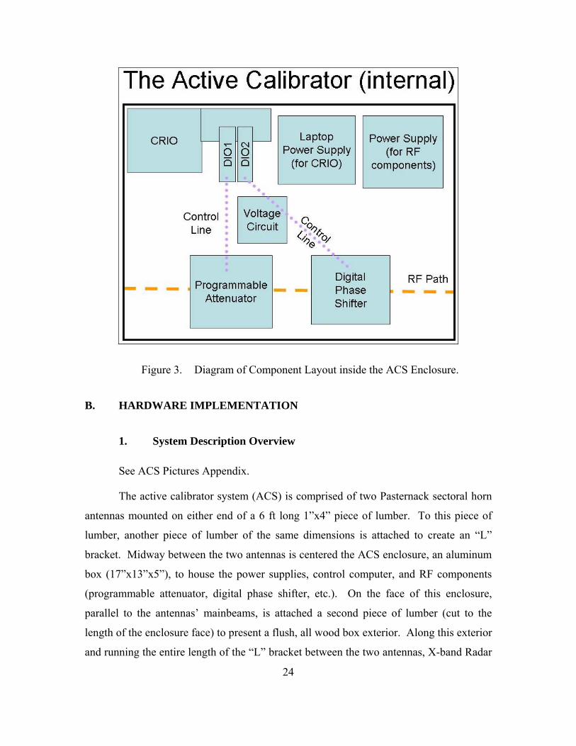
24
Figure 3. Diagram of Component Layout inside the ACS Enclosure.
B. HARDWARE IMPLEMENTATION
1. System Description Overview
See ACS Pictures Appendix.
The active calibrator system (ACS) is comprised of two Pasternack sectoral horn
antennas mounted on either end of a 6 ft long 1”x4” piece of lumber. To this piece of
lumber, another piece of lumber of the same dimensions is attached to create an “L”
bracket. Midway between the two antennas is centered the ACS enclosure, an aluminum
box (17”x13”x5”), to house the power supplies, control computer, and RF components
(programmable attenuator, digital phase shifter, etc.). On the face of this enclosure,
parallel to the antennas’ mainbeams, is attached a second piece of lumber (cut to the
length of the enclosure face) to present a flush, all wood box exterior. Along this exterior
and running the entire length of the “L” bracket between the two antennas, X-band Radar
25
Absorbent Material (RAM) is attached. Although this RAM has its greatest RF
absorbency at 9.4 GHz, it provides sufficient RF absorbency across the entire RF range of
interest, 9-10 GHz, to reduce undesired RF returns greater in power than the transmitted
power of the ACS’s transmit antenna output. This RAM is sectioned into three pieces
(two 24”x10”x2” and one 19”x9”x2”). Each piece is attached via removable Velcro to
aid in transport and storage. The antennas are mounted and oriented to transmit and
receive horizontally polarized signals. They are connected to the enclosure via 3 ft RF
cables. All of the ACS’s components apart from the antennas are contained inside the
enclosure.
2. Hardware List
External Hardware (Quantity/Description/Dimensions, if applicable)
(1) Aluminum box(enclosure) (17”x13”x5”) (3) Pieces Emerson & Cuming AN77 RAM (two, left and right side, 24”x10”x2” and
one, center, 19”x9”x2”) (3) Pieces lumber (1”x4”, two 6 ft long and one 19” long) (2) Pasternack Sectoral Horn Antennas (2) Pasternack semi-flexible RF Cables (3 ft) (1) Ethernet (RJ-45) Cable (1) Dell Precision M65 with 2.33 GHz Core 2 Duo Processor, 2GB 667 MHz RAM, 80
GB HDD Laptop and Dell 90W-AC Power Supply (1) AC Power Cable Miscellaneous Mounting Hardware (nuts, screws, washers, bolts, etc.)
Internal Hardware (Quantity/Description)
(1) Laptop Power Supply (24V CUI EA1050B-240) (1) Condor DC Power Supply (GLC-50A) (2) 25-pin-to-15-pin Control/Power Cables (1) Voltage Regulator Circuit (1) National Instruments Control Computer (CompactRIO Model Line to include: (1)
real-time controller, (1) reconfigurable embedded chassis, and (2) I/O modules)
3. Voltage Regulator Circuit
A voltage regulator circuit was required to convert the DC power supplied by the
Condor power supply (-15VDC, +15VDC, and +5VDC) to the additional voltages (-
5VDC and +12VDC) required by the RF components.
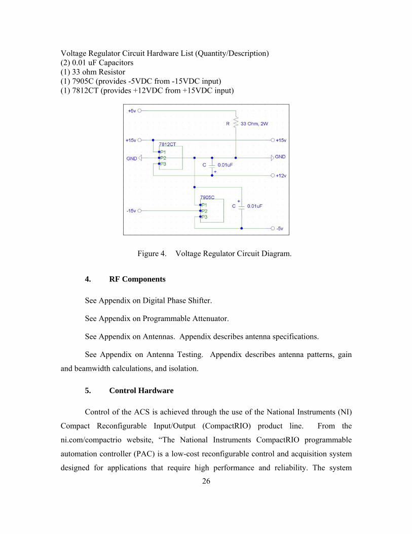
26
Voltage Regulator Circuit Hardware List (Quantity/Description) (2) 0.01 uF Capacitors (1) 33 ohm Resistor (1) 7905C (provides -5VDC from -15VDC input) (1) 7812CT (provides +12VDC from +15VDC input)
Figure 4. Voltage Regulator Circuit Diagram.
4. RF Components
See Appendix on Digital Phase Shifter.
See Appendix on Programmable Attenuator.
See Appendix on Antennas. Appendix describes antenna specifications.
See Appendix on Antenna Testing. Appendix describes antenna patterns, gain
and beamwidth calculations, and isolation.
5. Control Hardware
Control of the ACS is achieved through the use of the National Instruments (NI)
Compact Reconfigurable Input/Output (CompactRIO) product line. From the
ni.com/compactrio website, “The National Instruments CompactRIO programmable
automation controller (PAC) is a low-cost reconfigurable control and acquisition system
designed for applications that require high performance and reliability. The system
27
combines an open embedded architecture with small size, extreme ruggedness, and hot-
swappable industrial I/O modules. NI CompactRIO is powered by reconfigurable I/O
(RIO) FPGA technology.” Again from the ni.com/pac website, “PACs combine
programmable logic controller (PLC) ruggedness with PC functionality under an open,
flexible software architecture.”
The CompactRIO products used by the ACS include: a real-time controller, a
reconfigurable embedded chassis, and two I/O modules for digital input. Software
development was done on a Windows PC laptop with NI’s Developer Suite with Real-
time deployment and FPGA deployment options installed. Through this developer suite
and these options, all software development was done in the NI LabVIEWTM visual
programming language. For items not run on either the laptop’s Windows O/S or the
real-time controller’s real-time O/S, LabVIEW was auto-complied into the VHSIC
Hardware Description Language (VHDL) and run on the reconfigurable embedded
chassis. This process was seamless to the developer and no specific knowledge of VHDL
was required. These items included all of the software control required to manipulate the
phase shifter and programmable attenuator on a time scale at or near its fastest possible
switching speed. A normal O/S or real-time O/S is incapable of this speed of control
requiring the use of Field Programmable Gate Arrays (FPGAs).
See Appendix on CompactRIO.
6. Hardware Limitations
There are a few hardware limitations associated with the ACS. These limitations
affect the maximum possible Doppler shift and therefore radial velocity and velocity
spread that can be practically generated. Limited factors are dictated by the switching
speed of the programmable attenuator (300 ns) and phase shifter (500 ns), the CRIO
FPGA clock (25ns), and the response time of the digital I/O module (100 ns). Obviously,
the switching speeds of the programmable attenuator and phase shifter are the true
limiting factors as the CRIO components are more than capable of switching states at or
faster than the fastest switching speeds of both RF components.
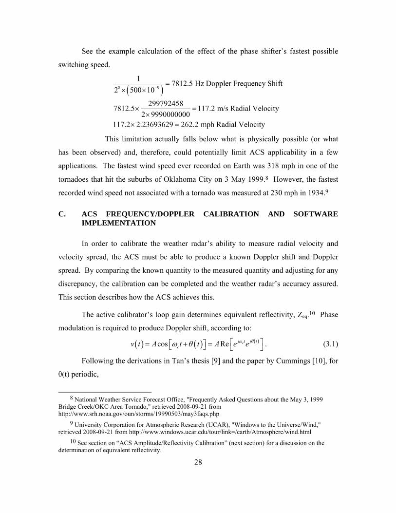
28
See the example calculation of the effect of the phase shifter’s fastest possible
switching speed.
( )8 9
1 7812.5 Hz Doppler Frequency Shift2 500 10
2997924587812.5 117.2 m/s Radial Velocity2 9990000000
117.2 2.23693629 262.2 mph Radial Velocity
−=
× ×
× =×
× =
This limitation actually falls below what is physically possible (or what
has been observed) and, therefore, could potentially limit ACS applicability in a few
applications. The fastest wind speed ever recorded on Earth was 318 mph in one of the
tornadoes that hit the suburbs of Oklahoma City on 3 May 1999.8 However, the fastest
recorded wind speed not associated with a tornado was measured at 230 mph in 1934.9
C. ACS FREQUENCY/DOPPLER CALIBRATION AND SOFTWARE IMPLEMENTATION
In order to calibrate the weather radar’s ability to measure radial velocity and
velocity spread, the ACS must be able to produce a known Doppler shift and Doppler
spread. By comparing the known quantity to the measured quantity and adjusting for any
discrepancy, the calibration can be completed and the weather radar’s accuracy assured.
This section describes how the ACS achieves this.
The active calibrator’s loop gain determines equivalent reflectivity, Zeq.10 Phase
modulation is required to produce Doppler shift, according to:
( ) ( ) ( )cos Re c j tj tcv t A t t A e e θωω θ ⎡ ⎤= + =⎡ ⎤⎣ ⎦ ⎣ ⎦ . (3.1)
Following the derivations in Tan’s thesis [9] and the paper by Cummings [10], for
θ(t) periodic,
8 National Weather Service Forecast Office, "Frequently Asked Questions about the May 3, 1999
Bridge Creek/OKC Area Tornado," retrieved 2008-09-21 from http://www.srh.noaa.gov/oun/storms/19990503/may3faqs.php
9 University Corporation for Atmospheric Research (UCAR), "Windows to the Universe/Wind," retrieved 2008-09-21 from http://www.windows.ucar.edu/tour/link=/earth/Atmosphere/wind.html
10 See section on “ACS Amplitude/Reflectivity Calibration” (next section) for a discussion on the determination of equivalent reflectivity.
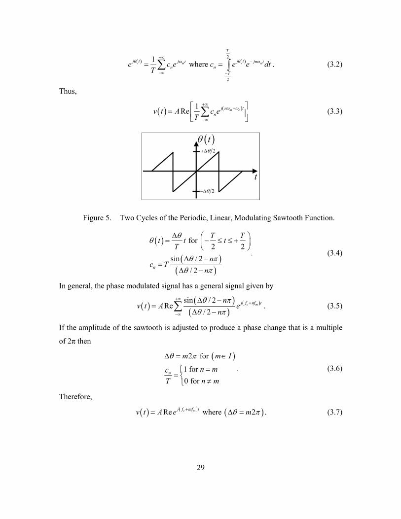
29
( ) ( )2
2
1 where m m
T
j t j tj t jn tn n
T
e c e c e e dtT
θ θω ω+∞
−
−∞ −
= =∑ ∫ . (3.2)
Thus,
( ) ( )1Re m cj n tnv t A c e
Tω ω
+∞+
−∞
⎡ ⎤= ⎢ ⎥⎣ ⎦∑ (3.3)
Figure 5. Two Cycles of the Periodic, Linear, Modulating Sawtooth Function.
( )
( )( )
for 2 2
sin / 2/ 2n
T Tt t tT
nc T
n
θθ
θ πθ π
Δ ⎛ ⎞= − ≤ ≤ +⎜ ⎟⎝ ⎠
Δ −=
Δ −
. (3.4)
In general, the phase modulated signal has a general signal given by
( ) ( )( )
( )sin / 2Re
/ 2c mj f nf tn
v t A en
θ πθ π
+∞+
−∞
Δ −=
Δ −∑ . (3.5)
If the amplitude of the sawtooth is adjusted to produce a phase change that is a multiple
of 2π then
( )2 for
1 for 0 for
n
m m I
n mcn mT
θ πΔ = ∈
=⎧= ⎨ ≠⎩
. (3.6)
Therefore,
( ) ( ) ( )Re where 2c mj f mf tv t A e mθ π+= Δ = . (3.7)
30
The real part of the complex exponential expression is cosine with argument indicating
the translation (Doppler shift) from frequency cf to frequency c mf mf+ . In other words,
each spectral line is separated by the modulating frequency and lines exist symmetrically
above and below the carrier.
By cycling through 360° (2π) of phase at this periodic rate a known
frequency/Doppler shift is produced against which the weather radar can be calibrated.
This periodic phase cycling (and thus frequency translation) is implemented in the ACS
using a digital phase shifter. However, there are imperfections associated with this
method. Imperfect implementation results in spurious sidebands due to finite sawtooth
flyback time, incorrect sawtooth amplitude, the digital staircase approximation to linear
phase shift, phase error, and finite phase shifter switching time.[10]
Again, following the derivations in the thesis by Tan [8], for a digital phase shifter
using N=2B steps,
( ) ( ) ( )( ) ( )1 sin /
cos1 /
m
c mK
Nv t A K t
mN Nπ
ω ωπ
+∞
=−∞
−= +
+∑ (3.8)
where 1K mN= + and m is an integer. The frequencies of the non-zero spectral
components are given by c mf f Kf= + or ( )1c mf f mN f= + + . The amplitude of the Kth
sideband relative to the input carrier is given by
2 2
22
0
/ 2/ 2
KKK
C AP CP A
= = . (3.9)
The first sideband in the spectrum of the translated signal is
( ) ( )( ) ( )1
sin /cos
/ c m
Nv t A K t
Nπ
ω ωπ
= + . (3.10)
The translation loss is defined as
( )( )
( )( )
sin / 2sin /20 log 20log
/ / 2
B
dB B
NTL
Nππ
π π
⎡ ⎤⎡ ⎤⎢ ⎥= − = −⎢ ⎥⎢ ⎥⎣ ⎦ ⎣ ⎦
. (3.11)
This loss rapidly approaches 0 dB as the number of bits of phase shift increase. If B=4
bits, for example, TLdB=0.06 dB.
31
The amplitudes of the undesired sidebands are also of interest. The undesired
sideband with the highest amplitude is 1K N= − + . Relative to the desired sideband,
K=1, the suppression ratio is
( ) ( )20log 1 20log 2 1BBSR N= − = − . (3.12)
The suppression ratio also improves rapidly as the number of bits is increased. If N= 4,
for example, SRdB= 23.5 dB.
See Appendix I on LabVIEW for the Digital Phase Shifter which gives further
explanation of how the phase shifter is controlled by the CompactRIO to produce the 2π
periodic phase cycling.
In conclusion, one of the primary advantages of the ACS is its ability to introduce
Doppler shift. This permits the calibrator signal to be extracted from mainbeam ground
clutter at elevation angles near zero and from sidelobe clutter at higher elevation angles.
In most cases, convenience will dictate that the ACS be operated near the ground.
D. ADDING VELOCITY SPREAD
Velocity spread can be added to the Doppler shifted signal by varying the
frequency of the sawtooth waveform used in the phase modulator. The frequency should
be varied in accordance with a Gaussian random variable that has been low pass filtered
to produce a modulating signal with the desired correlation time. This functionality was
not fully implemented in the ACS at the conclusion of this study. See Chapter IV on
Future Work.
E. ACS AMPLITUDE/REFLECTIVITY CALIBRATION
In order to calibrate the weather radar’s ability to measure reflectivity, the ACS
must be able to reliably simulate a known reflectivity. This is accomplished by receiving
the incident radar signal and retransmitting a signal of known power relative to the
incident signal. From a measurement of the echo signal power received by the radar and
knowledge of the ACS loop gain, the calibration can be completed and the weather
32
radar’s absolute accuracy in amplitude assured. This section describes how the ACS is
calibrated so it can in turn be used to calibrate a weather radar.
1. Measurement Premise
The ACS needs to produce a power density equivalent to that scattered by a target
of known RCS. This power will be the effective radiated power (or ERP) of the ACS.
The ERP of the ACS will be a function of (depend on) the ERP of the radar. This is
because the ACS does not produce an ERP from an independent/internal power source,
but rather as acts a repeater (and modifier) of the power received from the radar.
The power received from the radar will depend on the ERP of the radar and the
losses involved between the ACS and the radar. At this radar frequency, the losses
between the ACS and the radar will primarily depend on the distance between the ACS
and the radar (spreading loss or free space loss only, unless a ground reflection is present
as will be the case for elevation angles near zero) and atmospheric attenuation
(propagation loss), but also losses internal to the radar (system losses which cannot be
precisely known). Those losses which depend on distance will affect the reflectivity
observed by the radar due to the calibrator twice – first, as the ERP of the radar is
affected on its way to becoming the received power of the calibrator and, second, as the
ERP of the calibrator is affected on its return to becoming the received power of the
radar. While the spreading loss is well known (24 RL π
λ⎛ ⎞= ⎜ ⎟⎝ ⎠
) and can be accurately
calculated, the propagation loss is less well known (as it depends on many time variant
factors) and is more difficult to accurately calculate. In order to isolate this uncertainty at
any given time, the equivalent reflectivity of the ACS can be compared to a known
reflectivity at equal distances and with the propagation losses minimized as much as
possible (as in an anechoic chamber). By comparing these two values, the equivalent
reflectivity of the ACS can be measured. Under these settings the losses internal to the
radar can be isolated (the system losses which cannot be precisely known will be
calibrated out).
33
An equation for the ERP of the ACS and thereby the equivalent reflectivity of the
ACS can be defined as a function of the received power of the ACS (from the radar) and
the loop gain (system gain and losses) of the ACS. These include the gain of both
antennas (transmit and receive), cable losses, phase shifter losses, programmable
attenuator losses, isolator losses, amplifier gain, and other RF components’ losses (only
the amplifier provides gain). On the whole, the ACS’s ERP and therefore its equivalent
reflectivity can be controlled (varied) by the programmable attenuator (variable
gain/loss). However, this is only effective as long as the net gain/loss of all of the ACS’s
RF components (fixed gain/loss) in total exceed the reflectivity of the ACS due to its
exposed surface area.
The equivalent reflectivity due to the ACS’s transmit antenna is in direct
competition with the actual reflectivity due to the ACS’s surface area. Both depend on
the radar ERP, but the equivalent reflectivity further depends on the ACS’s loop gain
acting to re-radiate the radar’s power while the actual reflectivity depends on the exposed
surface area of the ACS (to include all sides facing the radar) acting to reflect the radar’s
power. If the controlled power does not exceed this value, variable amplitude calibration
(as will be needed for amplitude statistics) will not be possible. Instead, only a single
reflectivity (the actual reflectivity) of the ACS will ever be observed by the radar. This is
the same principle used in passive calibration systems (such as the balloon and sphere)
where a controlled Doppler calibration is not possible. Radar Absorbent Material (RAM)
was used to reduce the actual reflectivity to levels below the equivalent reflectivity. See
Chapter III, Section B, Subsection 1 for further details on RAM use.
2. Measurement Method
What follows is the method used to calibrate out these unknown system losses for
accurate reflectivity measurements (estimates) by the weather radar based on the
equivalent RCS of the ACS. See Chapter II, Section F, on “Radar Principles and
Weather Radar Equation Correction” for background and supporting theory directly
applicable to this process and these calculations. The following development shows how
the equivalent RCS of the ACS was experimentally determined through anechoic
34
chamber measurements and subsequent calculations to satisfy a most fundamental radar
calibration requirement – namely, that the ACS’s equivalent RCS must be known [5].
As mentioned before, the value of the equivalent reflectivity (or more accurately
equivalent radar cross section or RCS) of the ACS can be measured and calculated in
comparison to a known reflectivity (or RCS) of another target. In this study, an
aluminum sphere was used and measurements made inside an anechoic chamber at a
fixed, known distance to serve as the known reflectivity. A 12” diameter aluminum
sphere was chosen out of three diameters available based on the initial calculations and
estimates performed below.
a. Initial Calculations
Prior to making measurements in the anechoic chamber theoretical
calculations were made using approximately known or individually measured values of
the required quantities. The signal source in the anechoic chamber was a vector network
analyzer (VNA). The VNA replaces the radar as the signal source when calibrating the
ACS in the anechoic chamber.
Below is a list of constants, either measured or known, to include:
R, the measured one-way distance from the transmit and receive antennas to the ACS inside the anechoic chamber. (measured) f, the radio center frequency. (known, selected on vector network analyzer or VNA) c, the speed of light. (known) λ, the wavelength. (calculated) Pt, the VNA transmit power a.k.a. the power input to the anechoic transmit antenna from the VNA to include all losses from the output of the VNA to the antenna (cabling, etc.). (known, selected on VNA) Gt=Gr, the gain of the VNA antenna – one in the same - a.k.a. the anechoic transmit and receive antennas - both the same. (measured, See Appendices on Antennas.) EIRP, the radar’s Effective Isotropic Radiated Power. The product of the transmit power and antenna gain. (calculated) Gc, the calibrator’s antenna gain. Both antennas on the calibrator are the same. (measured, See Appendices E and F on Antennas.) Gamp, the calibrator’s loop gain to include all system losses (cabling, phase shifter while not phase shifting, connectors, etc.) – i.e. net gain. The actual gain of the amplifier used in the calibrator is +35 dB with -20 dB of system losses for +15 dB net. (calculated via measured values: amplifier gain and system losses) FSL, the Free Space Loss or Spreading Loss associated with the distance R. (calculated)
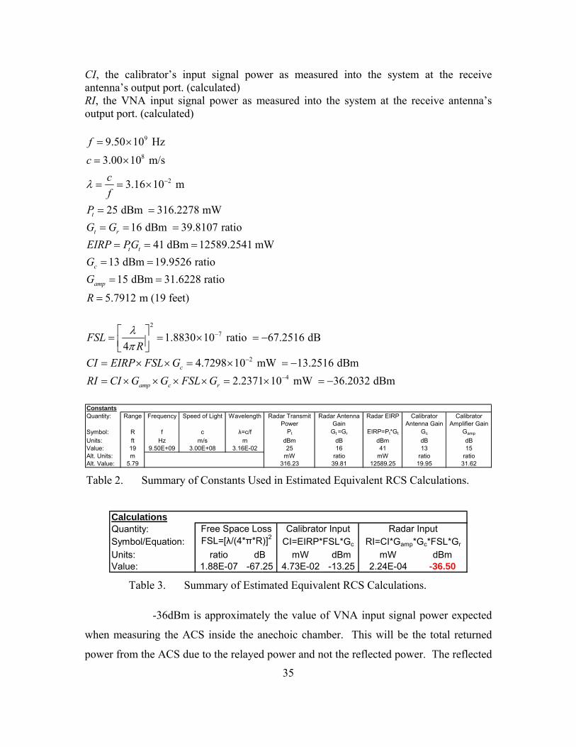
35
CI, the calibrator’s input signal power as measured into the system at the receive antenna’s output port. (calculated) RI, the VNA input signal power as measured into the system at the receive antenna’s output port. (calculated)
9
8
2
9.50 10 Hz3.00 10 m/s
3.16 10 m
25 dBm 316.2278 mW16 dBm 39.8107 ratio
41 dBm 12589.2541 mW13 dBm 19.9526 ratio
15 dBm 31.6228 ratio
5.7912 m (19 feet)
t
t r
t t
c
amp
fc
cf
PG GEIRP PGGG
R
λ −
= ×
= ×
= = ×
= =
= = == = =
= == =
=
2
71.8830 10 ratio 67.2516 dB4
FSLR
λπ
−⎡ ⎤= = × = −⎢ ⎥⎣ ⎦
24.7298 10 mW 13.2516 dBmcCI EIRP FSL G −= × × = × = − 42.2371 10 mW 36.2032 dBmamp c rRI CI G G FSL G −= × × × × = × = −
ConstantsQuantity: Range Frequency Speed of Light Wavelength Radar Transmit
PowerRadar Antenna
GainRadar EIRP Calibrator
Antenna GainCalibrator
Amplifier GainSymbol: R f c λ=c/f Pt Gt =Gr EIRP=Pt*Gt Gc Gamp
Units: ft Hz m/s m dBm dB dBm dB dBValue: 19 9.50E+09 3.00E+08 3.16E-02 25 16 41 13 15Alt. Units: m mW ratio mW ratio ratioAlt. Value: 5.79 316.23 39.81 12589.25 19.95 31.62 Table 2. Summary of Constants Used in Estimated Equivalent RCS Calculations.
CalculationsQuantity:Symbol/Equation:Units: ratio dB mW dBm mW dBmValue: 1.88E-07 -67.25 4.73E-02 -13.25 2.24E-04 -36.50
Radar InputRI=CI*Gamp*Gc*FSL*GrFSL=[λ/(4*π*R)]2
Free Space LossCI=EIRP*FSL*Gc
Calibrator Input
Table 3. Summary of Estimated Equivalent RCS Calculations.
-36dBm is approximately the value of VNA input signal power expected
when measuring the ACS inside the anechoic chamber. This will be the total returned
power from the ACS due to the relayed power and not the reflected power. The reflected
36
power is much smaller (no return was detected with the ACS in the anechoic chamber
and RAM attached) and has been minimized by the use of X-band Radar Absorbent
Material (RAM). Again, see Chapter III, Section B, Subsection 1 for further details on
RAM use.
The power received from the ACS must be compared to the received
power from a target of a known RCS to calculate an equivalent RCS for the ACS. The
known RCS that was used was that of a polished aluminum sphere. Three spheres were
available, a 3”, a 6” and a 12” diameter sphere. The expected received power was
calculated for all three. The relation for the monostatic RCS of a sphere in the optical
region (frequency region) was used. The power had to be great enough to be detected by
the VNA, but not so great as to cause saturation. The best suitable candidate from the
three available was found to be the 12” diameter sphere because of its larger (but not too
large, i.e. saturating) return amplitude. See example calculation below.
2
2 2
5
6 in 0.1524 m2 30.3 Optical Region (See Figure 6.)
1 for Optical Region (See Figure 6.)
7.2966 10 sm 11.3688 dBsmReceived Power 1.6338 10 mW 47.8679 dBm
aaa
aa
πβλ
σπσ π
= =
= = ⇒
=
= = × = −
= × = −
Following the example, for a 3” diameter sphere -59.909 dBm and for a 6” diameter
sphere -53.889 dBm.
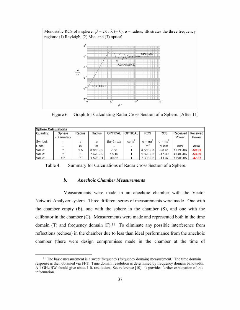
37
Figure 6. Graph for Calculating Radar Cross Section of a Sphere. [After 11]
Sphere CalculationsQuantity: Sphere
(Diameter)Radius Radius OPTICAL OPTICAL RCS RCS Received
PowerReceived
PowerSymbol: - a a βa=2πa/λ σ/πa2 σ = πa2 σ = πa2
Units: - in m - - m2 dBsm mW dBmValue: 3" 1.5 3.81E-02 7.58 1 4.56E-03 -23.41 1.02E-06 -59.91Value: 6" 3 7.62E-02 15.16 1 1.82E-02 -17.39 4.08E-06 -53.89Value: 12" 6 1.52E-01 30.32 1 7.30E-02 -11.37 1.63E-05 -47.87
Table 4. Summary for Calculations of Radar Cross Section of a Sphere.
b. Anechoic Chamber Measurements
Measurements were made in an anechoic chamber with the Vector
Network Analyzer system. Three different series of measurements were made. One with
the chamber empty (E), one with the sphere in the chamber (S), and one with the
calibrator in the chamber (C). Measurements were made and represented both in the time
domain (T) and frequency domain (F).11 To eliminate any possible interference from
reflections (echoes) in the chamber due to less than ideal performance from the anechoic
chamber (there were design compromises made in the chamber at the time of
11 The basic measurement is a swept frequency (frequency domain) measurement. The time domain
response is then obtained via FFT. Time domain resolution is determined by frequency domain bandwidth. A 1 GHz BW should give about 1 ft. resolution. See reference [10]. It provides further explanation of this information.
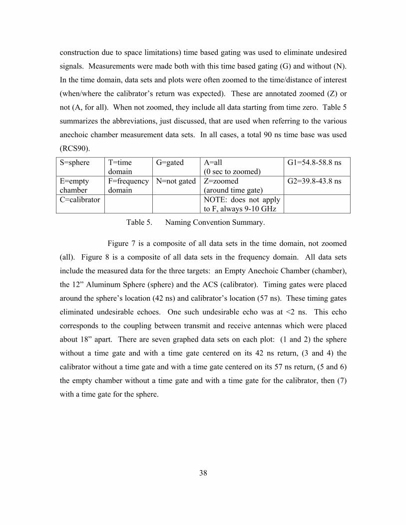
38
construction due to space limitations) time based gating was used to eliminate undesired
signals. Measurements were made both with this time based gating (G) and without (N).
In the time domain, data sets and plots were often zoomed to the time/distance of interest
(when/where the calibrator’s return was expected). These are annotated zoomed (Z) or
not (A, for all). When not zoomed, they include all data starting from time zero. Table 5
summarizes the abbreviations, just discussed, that are used when referring to the various
anechoic chamber measurement data sets. In all cases, a total 90 ns time base was used
(RCS90).
S=sphere T=time domain
G=gated A=all (0 sec to zoomed)
G1=54.8-58.8 ns
E=empty chamber
F=frequency domain
N=not gated Z=zoomed (around time gate)
G2=39.8-43.8 ns
C=calibrator NOTE: does not apply to F, always 9-10 GHz
Table 5. Naming Convention Summary.
Figure 7 is a composite of all data sets in the time domain, not zoomed
(all). Figure 8 is a composite of all data sets in the frequency domain. All data sets
include the measured data for the three targets: an Empty Anechoic Chamber (chamber),
the 12” Aluminum Sphere (sphere) and the ACS (calibrator). Timing gates were placed
around the sphere’s location (42 ns) and calibrator’s location (57 ns). These timing gates
eliminated undesirable echoes. One such undesirable echo was at <2 ns. This echo
corresponds to the coupling between transmit and receive antennas which were placed
about 18” apart. There are seven graphed data sets on each plot: (1 and 2) the sphere
without a time gate and with a time gate centered on its 42 ns return, (3 and 4) the
calibrator without a time gate and with a time gate centered on its 57 ns return, (5 and 6)
the empty chamber without a time gate and with a time gate for the calibrator, then (7)
with a time gate for the sphere.
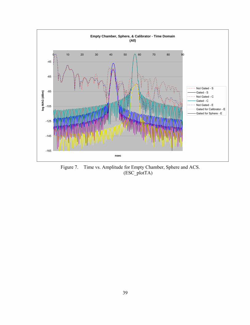
39
Empty Chamber, Sphere, & Calibrator - Time Domain(All)
-165
-145
-125
-105
-85
-65
-45
0 10 20 30 40 50 60 70 80 90
nsec
log
MA
G (d
Bm
)
Not Gated - SGated - SNot Gated - CGated - CNot Gated - EGated for Calibrator - EGated for Sphere - E
Figure 7. Time vs. Amplitude for Empty Chamber, Sphere and ACS.
(ESC_plotTA)
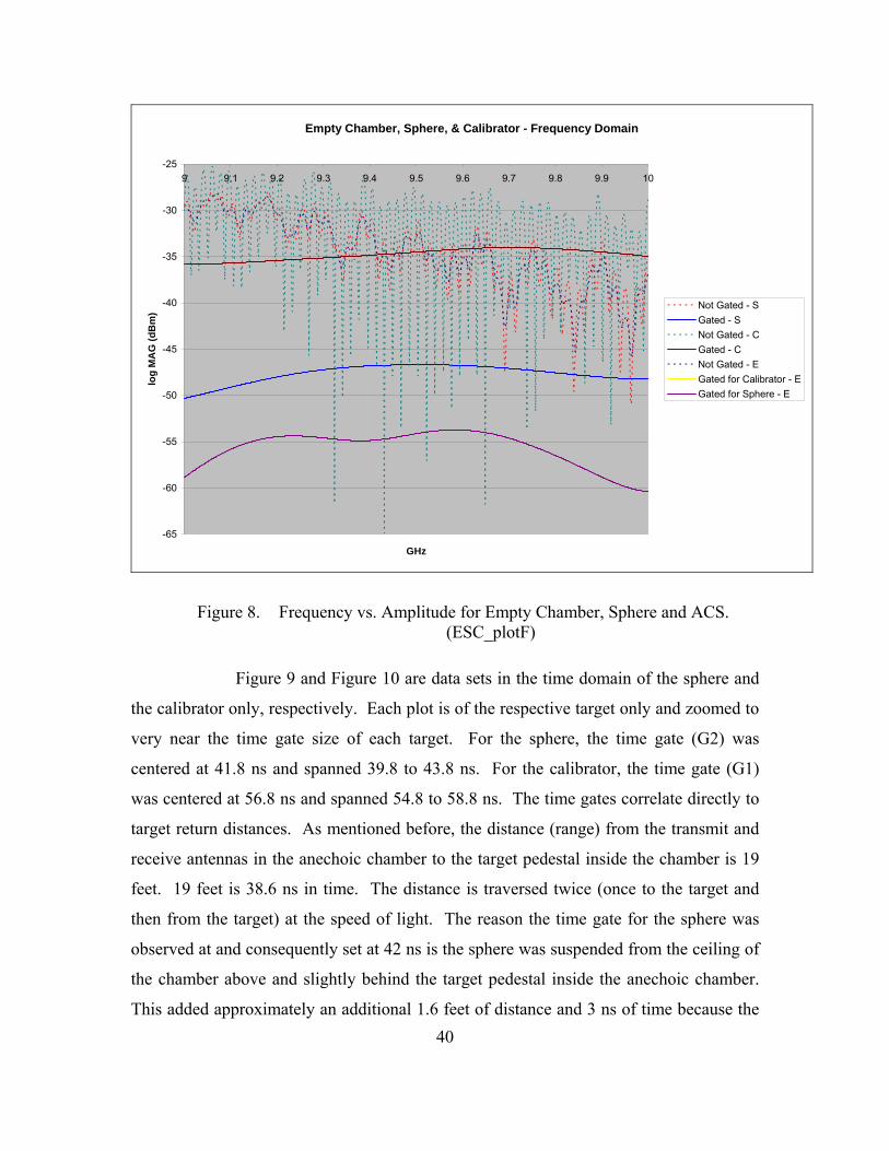
40
Empty Chamber, Sphere, & Calibrator - Frequency Domain
-65
-60
-55
-50
-45
-40
-35
-30
-259 9.1 9.2 9.3 9.4 9.5 9.6 9.7 9.8 9.9 10
GHz
log
MA
G (d
Bm
)
Not Gated - SGated - SNot Gated - CGated - CNot Gated - EGated for Calibrator - EGated for Sphere - E
Figure 8. Frequency vs. Amplitude for Empty Chamber, Sphere and ACS. (ESC_plotF)
Figure 9 and Figure 10 are data sets in the time domain of the sphere and
the calibrator only, respectively. Each plot is of the respective target only and zoomed to
very near the time gate size of each target. For the sphere, the time gate (G2) was
centered at 41.8 ns and spanned 39.8 to 43.8 ns. For the calibrator, the time gate (G1)
was centered at 56.8 ns and spanned 54.8 to 58.8 ns. The time gates correlate directly to
target return distances. As mentioned before, the distance (range) from the transmit and
receive antennas in the anechoic chamber to the target pedestal inside the chamber is 19
feet. 19 feet is 38.6 ns in time. The distance is traversed twice (once to the target and
then from the target) at the speed of light. The reason the time gate for the sphere was
observed at and consequently set at 42 ns is the sphere was suspended from the ceiling of
the chamber above and slightly behind the target pedestal inside the anechoic chamber.
This added approximately an additional 1.6 feet of distance and 3 ns of time because the
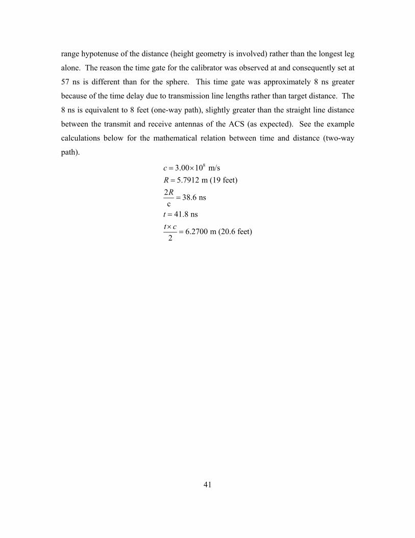
41
range hypotenuse of the distance (height geometry is involved) rather than the longest leg
alone. The reason the time gate for the calibrator was observed at and consequently set at
57 ns is different than for the sphere. This time gate was approximately 8 ns greater
because of the time delay due to transmission line lengths rather than target distance. The
8 ns is equivalent to 8 feet (one-way path), slightly greater than the straight line distance
between the transmit and receive antennas of the ACS (as expected). See the example
calculations below for the mathematical relation between time and distance (two-way
path). 83.00 10 m/s
5.7912 m (19 feet)2 38.6 nsc
41.8 ns
6.2700 m (20.6 feet)2
cR
R
tt c
= ×=
=
=×
=
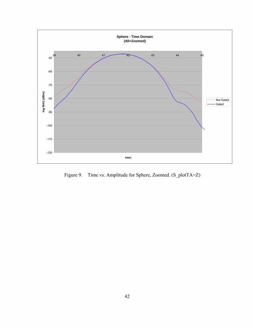
42
Sphere - Time Domain(All=Zoomed)
-120
-110
-100
-90
-80
-70
-60
-5039 40 41 42 43 44 45
nsec
log
MA
G (d
Bm
)
Not GatedGated
Figure 9. Time vs. Amplitude for Sphere, Zoomed. (S_plotTA=Z)
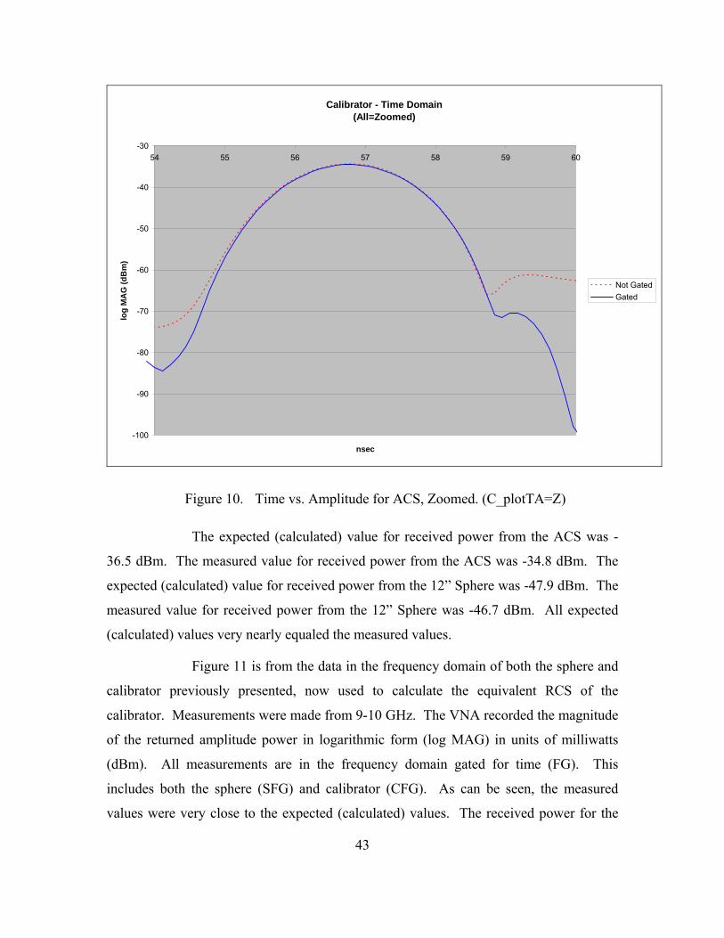
43
Calibrator - Time Domain(All=Zoomed)
-100
-90
-80
-70
-60
-50
-40
-3054 55 56 57 58 59 60
nsec
log
MA
G (d
Bm
)
Not GatedGated
Figure 10. Time vs. Amplitude for ACS, Zoomed. (C_plotTA=Z)
The expected (calculated) value for received power from the ACS was -
36.5 dBm. The measured value for received power from the ACS was -34.8 dBm. The
expected (calculated) value for received power from the 12” Sphere was -47.9 dBm. The
measured value for received power from the 12” Sphere was -46.7 dBm. All expected
(calculated) values very nearly equaled the measured values.
Figure 11 is from the data in the frequency domain of both the sphere and
calibrator previously presented, now used to calculate the equivalent RCS of the
calibrator. Measurements were made from 9-10 GHz. The VNA recorded the magnitude
of the returned amplitude power in logarithmic form (log MAG) in units of milliwatts
(dBm). All measurements are in the frequency domain gated for time (FG). This
includes both the sphere (SFG) and calibrator (CFG). As can be seen, the measured
values were very close to the expected (calculated) values. The received power for the
44
12” Aluminum Sphere was calculated to be -47.87 dBm and observed to be near -47
dBm. The received power for the calibrator was calculated to be -36.50 dBm and
observed to be near -35 dBm. The RCS of the sphere was previously calculated to be
-11.37 dBsm (S–RCS). To calculate the RCS of the calibrator (C–RCS) based on the
observed/measured data, the CFG - SFG=Δ (dB) was added to the sphere’s RCS. Over
the entire frequency band the C–RCS varied from 0.6 to 3.2 dBsm. Note all these
measurements in the chamber included the use of the RF amplifier within the calibrator
system. When used with the weather radar, signal levels are great enough and ranges
short enough such that an RF amplifier is not needed. Furthermore, calculations are
made to make sure the signal return to the radar is in the proper range to prevent receiver
saturation.
Equivalent RCS of Calibrator(with in-line amplifier)
0.5
1
1.5
2
2.5
3
3.5
9 9.1 9.2 9.3 9.4 9.5 9.6 9.7 9.8 9.9 10
Frequency (GHz)
RC
S (s
igm
a) in
dB
sm
Figure 11. Frequency vs. Equivalent RCS of the ACS. (RCS_plot)
With these measured values the equivalent RCS of the ACS was observed
to range from 0.6 to 3.2 dBsm across the 9-10 GHz RF band. On average (mean), the
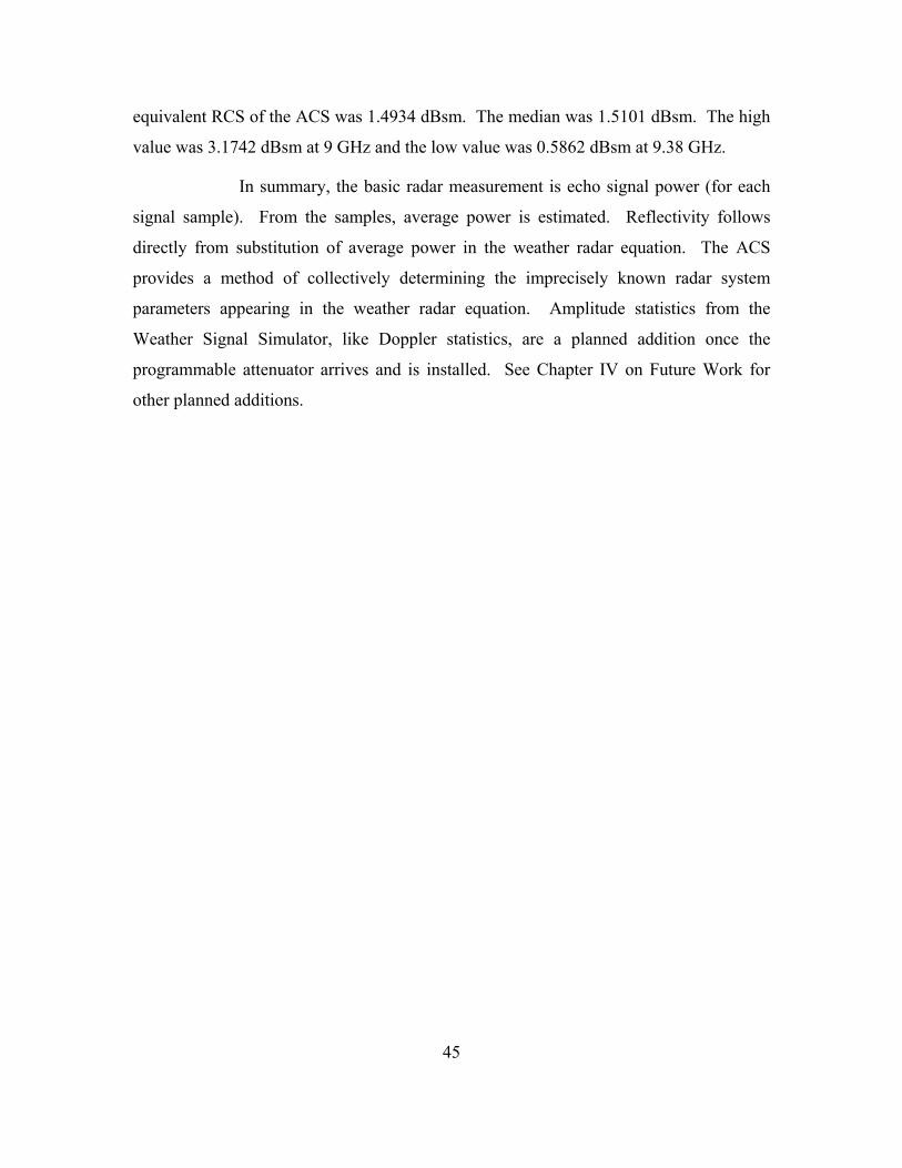
45
equivalent RCS of the ACS was 1.4934 dBsm. The median was 1.5101 dBsm. The high
value was 3.1742 dBsm at 9 GHz and the low value was 0.5862 dBsm at 9.38 GHz.
In summary, the basic radar measurement is echo signal power (for each
signal sample). From the samples, average power is estimated. Reflectivity follows
directly from substitution of average power in the weather radar equation. The ACS
provides a method of collectively determining the imprecisely known radar system
parameters appearing in the weather radar equation. Amplitude statistics from the
Weather Signal Simulator, like Doppler statistics, are a planned addition once the
programmable attenuator arrives and is installed. See Chapter IV on Future Work for
other planned additions.

46
THIS PAGE INTENTIONALLY LEFT BLANK
47
IV. CONCLUSION AND FUTURE WORK
A. CONCLUSION
An active calibration system (ACS) for weather radar was successfully designed
and implemented. The ACS was verified to be a functional weather radar active
calibration system under laboratory testing. It successfully provided the means (met the
requirements) to verify all three of the signal parameters measured (estimated) by a
weather radar. These include the zeroth Doppler moment (reflectivity), first Doppler
moment (average radial velocity), and second Doppler moment (velocity spread).
The cross-section (σ, or equivalent RCS) of the ACS and therefore the means to
measure and calculate the radar calibration constant (for reflectivity according to
Equation (2.31)) was successfully determined. The underlying data to calculate the
cross-section was measured and based on subsequent calculations determined to vary
from 0.6 to 3.2 dBsm across the frequency band of interest.
A constant Doppler shift (radial velocity) created by the ACS was observed and
verified by the visual inspection of several independent human operators using a
spectrum analyzer. The ACS successfully produced a known, operator selected radial
velocity. While it was not possible to observe a variable Doppler shift (velocity spread)
in exactly the same manner because of time scale limitations, the method to produce a
variable Doppler shift was manually verified in a similar manner. The ACS produced an
observable constant Doppler shift when provided a variable Doppler data file containing
several entries of the same Doppler shift rather than several entries each of a different
Doppler shift. If the control software read and executed each Doppler shift entry
(regardless of whether they were all the same) and produced the corresponding Doppler
shift (which could be observed), there is no reason to believe the control software would
not read and execute each Doppler shift entry (when they are different) to potentially
produce the corresponding varying Doppler shifts that are desired in the same manner as
was demonstrated for the test fixture. Based on this, the ACS was deemed to have
successfully produced a known velocity spread.
48
When tested with the MWR-05XP weather radar this should be sufficient to
remove system bias from the reflectivity estimate and to check the accuracy of mean
radial velocity and velocity spread estimates.
B. FUTURE WORK
The first item for future work is to field test the active calibrator system (ACS)
with the MWR-05XP. It should be tested to see if the constant Doppler generated by the
ACS is observed by the MWR-05XP. Then, a variable Doppler should be generated by
the ACS and to see if the MWR-05XP observes a Doppler spread. It should also be
tested to see if the equivalent RCS/Reflectivity measured is observed as expected and
then compared to the radar calibration constants obtained from the balloon and sphere
calibration system.
The active calibrator system was not entirely fabricated when this thesis research
was concluded. The programmable attenuator had not yet been received. Once received,
the programmable attenuator will need to be installed. New RF cables will have to be
fabricated to route the RF path sequentially through the phase shifter and programmable
attenuator. A control/power cable will have to be fabricated to link the CRIO’s DIO
module and the DC power supply voltages from the voltage regulator circuit with the
programmable attenuator. This cable will be the same type (25-pin to 15-pin) as the one
used for the same purposes by the phase shifter differing only by pin assignments. The
parts to fabricate this cable have already been procured and received.
The control software for the programmable attenuator has, for the most part,
already been written. The control software to independently control the programmable
attenuator is the same as for the phase shifter. It need only be duplicated with minor
modifications (e.g. filename for Reflectivity values vs. filename for Doppler values,
MATLAB script to convert Reflectivity to amplitude shifts vs. Doppler values to phase
shifts, etc.). All of the LabVIEW code could be duplicated with minor modifications and
run separately to control the programmable attenuator in the same manner as the phase
shifter (both 8-bit). In its current state, the ACS can calibrate the MWR-05XP for a
single constant amplitude return (Reflectivity) and multiple variable Doppler values.
49
With the addition of duplicate control code and the addition of the programmable
attenuator, the ACS can be configured to calibrate the MWR-05XP for multiple variable
amplitude returns to simulate the changes in pulse amplitude that would be observed.
However, controlling these values independently (one and then the other) does not allow
a calibrator to simulate “real world” weather conditions. In order to calibrate the radar
with “real world” weather conditions amplitude and phase values must be controlled
simultaneously and dependently. To do this, the control code for both the programmable
attenuator and phase shifter must be timed together. This can be achieved by controlling
the programmable attenuator and phase shifter from within the same control code. This
is slightly less straight forward than the minor modifications for independent control of
the two devices. However, it is possible and desirable. The existing phase shifter control
code would have to be modified to contain duplicate control subroutines for the
programmable attenuator from within its own control code. The difference would
primarily be the additional use of nested loops and sequence frames from with the same
control code (LabVIEW VI). With implementation of this simultaneous dependent
control “real world” weather signal statistics could be simulated by the phase and
amplitude variation of the ACS.
Testing of these “real world” weather patterns with the MWR-05XP is the final
objective. However, the ACS could and should be tested incrementally with the MWR-
05XP at various times as new features are implemented. It is suggested that the MWR-
05XP and ACS be tested together first, “as-is” (with the phase shifter installed only), then
after the addition of the programmable attenuator and added ability to control both the
phase shifter and programmable attenuator simultaneously. Final testing would occur
after all features are fully implemented and integrated into the ACS (to include output of
amplitude and Doppler statistics of “real world” weather patterns from the Weather
Signal Simulator).
In summary outline, Future Work should include:
1. A test of the ACS with the MWR-05XP in its current state (at the close of
this thesis research).
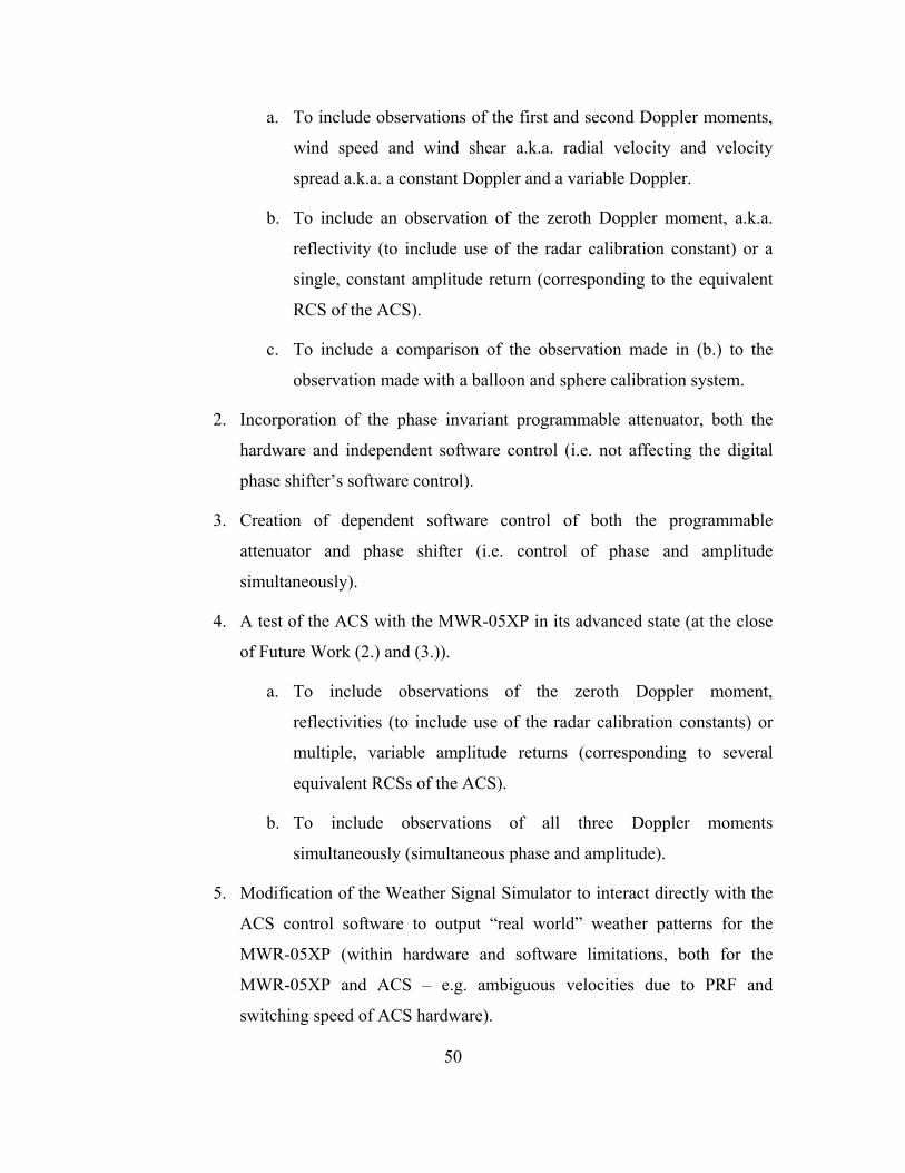
50
a. To include observations of the first and second Doppler moments,
wind speed and wind shear a.k.a. radial velocity and velocity
spread a.k.a. a constant Doppler and a variable Doppler.
b. To include an observation of the zeroth Doppler moment, a.k.a.
reflectivity (to include use of the radar calibration constant) or a
single, constant amplitude return (corresponding to the equivalent
RCS of the ACS).
c. To include a comparison of the observation made in (b.) to the
observation made with a balloon and sphere calibration system.
2. Incorporation of the phase invariant programmable attenuator, both the
hardware and independent software control (i.e. not affecting the digital
phase shifter’s software control).
3. Creation of dependent software control of both the programmable
attenuator and phase shifter (i.e. control of phase and amplitude
simultaneously).
4. A test of the ACS with the MWR-05XP in its advanced state (at the close
of Future Work (2.) and (3.)).
a. To include observations of the zeroth Doppler moment,
reflectivities (to include use of the radar calibration constants) or
multiple, variable amplitude returns (corresponding to several
equivalent RCSs of the ACS).
b. To include observations of all three Doppler moments
simultaneously (simultaneous phase and amplitude).
5. Modification of the Weather Signal Simulator to interact directly with the
ACS control software to output “real world” weather patterns for the
MWR-05XP (within hardware and software limitations, both for the
MWR-05XP and ACS – e.g. ambiguous velocities due to PRF and
switching speed of ACS hardware).
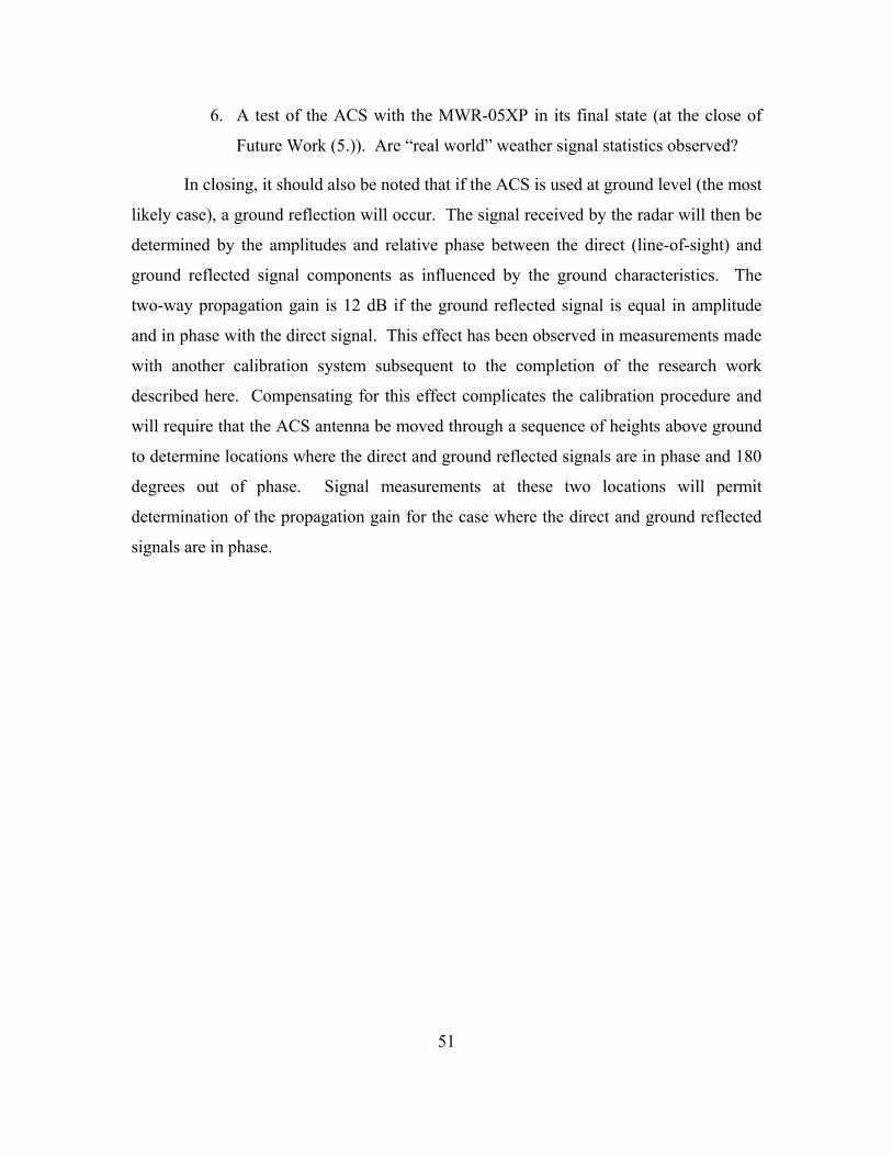
51
6. A test of the ACS with the MWR-05XP in its final state (at the close of
Future Work (5.)). Are “real world” weather signal statistics observed?
In closing, it should also be noted that if the ACS is used at ground level (the most
likely case), a ground reflection will occur. The signal received by the radar will then be
determined by the amplitudes and relative phase between the direct (line-of-sight) and
ground reflected signal components as influenced by the ground characteristics. The
two-way propagation gain is 12 dB if the ground reflected signal is equal in amplitude
and in phase with the direct signal. This effect has been observed in measurements made
with another calibration system subsequent to the completion of the research work
described here. Compensating for this effect complicates the calibration procedure and
will require that the ACS antenna be moved through a sequence of heights above ground
to determine locations where the direct and ground reflected signals are in phase and 180
degrees out of phase. Signal measurements at these two locations will permit
determination of the propagation gain for the case where the direct and ground reflected
signals are in phase.

52
THIS PAGE INTENTIONALLY LEFT BLANK
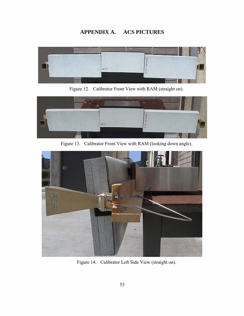
53
APPENDIX A. ACS PICTURES
Figure 12. Calibrator Front View with RAM (straight on).
Figure 13. Calibrator Front View with RAM (looking down angle).
Figure 14. Calibrator Left Side View (straight on).
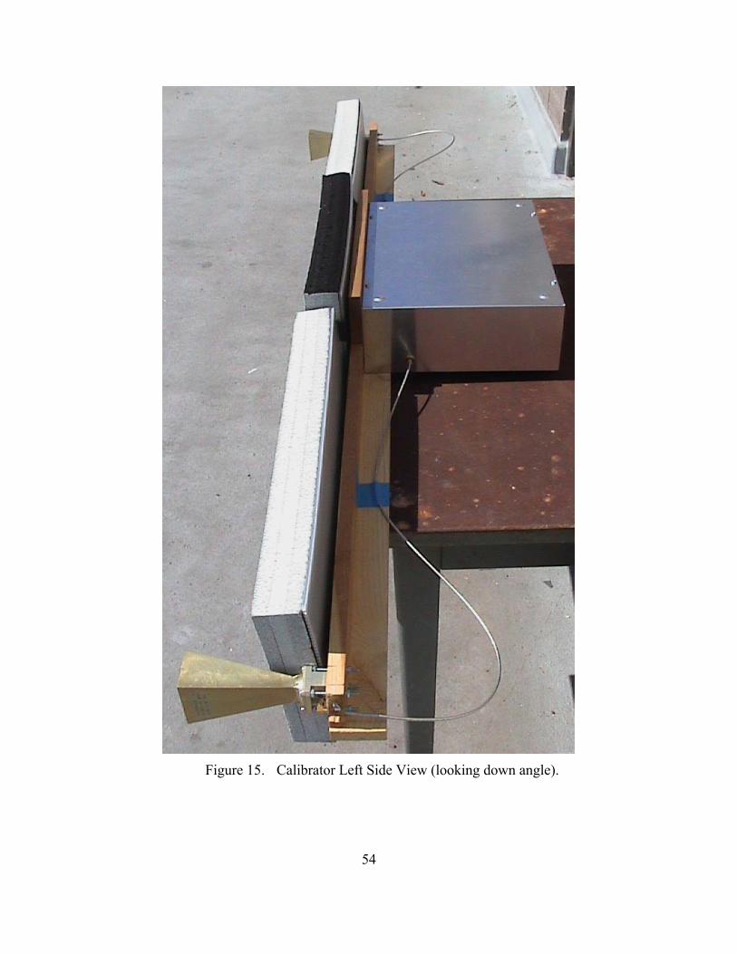
54
Figure 15. Calibrator Left Side View (looking down angle).
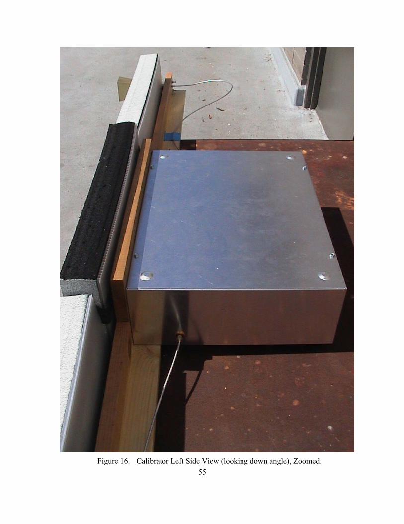
55
Figure 16. Calibrator Left Side View (looking down angle), Zoomed.
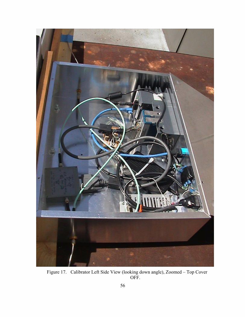
56
Figure 17. Calibrator Left Side View (looking down angle), Zoomed – Top Cover
OFF.
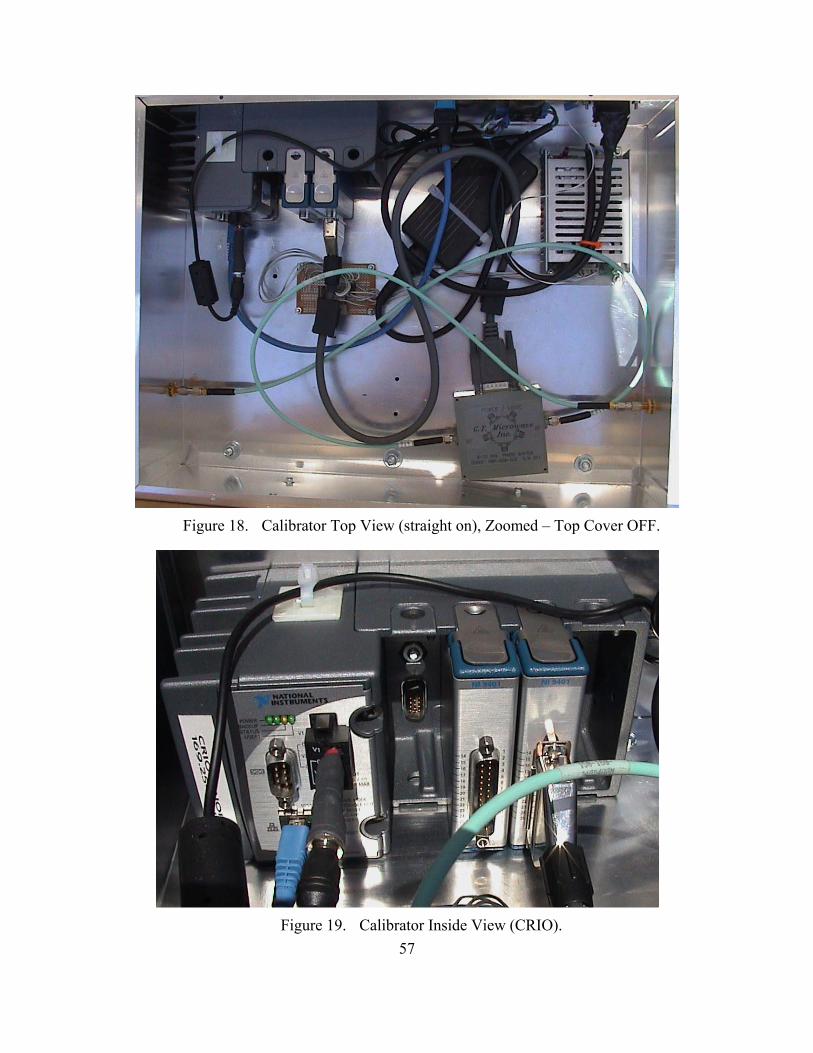
57
Figure 18. Calibrator Top View (straight on), Zoomed – Top Cover OFF.
Figure 19. Calibrator Inside View (CRIO).
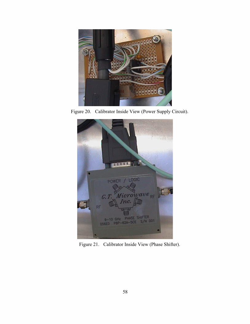
58
Figure 20. Calibrator Inside View (Power Supply Circuit).
Figure 21. Calibrator Inside View (Phase Shifter).
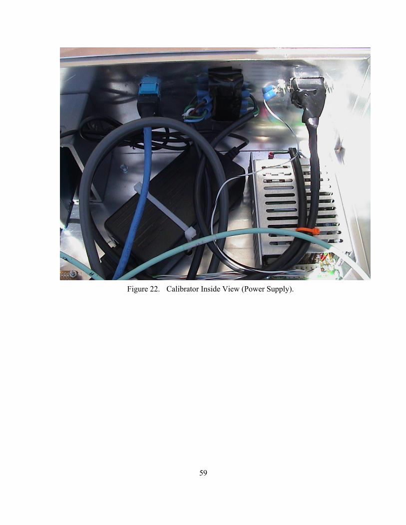
59
Figure 22. Calibrator Inside View (Power Supply).
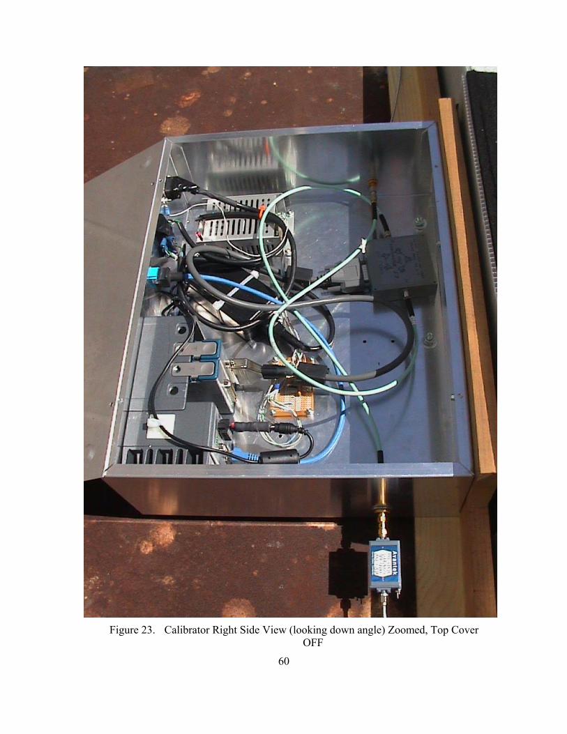
60
Figure 23. Calibrator Right Side View (looking down angle) Zoomed, Top Cover
OFF
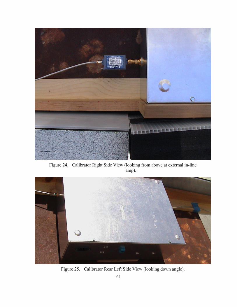
61
Figure 24. Calibrator Right Side View (looking from above at external in-line
amp).
Figure 25. Calibrator Rear Left Side View (looking down angle).
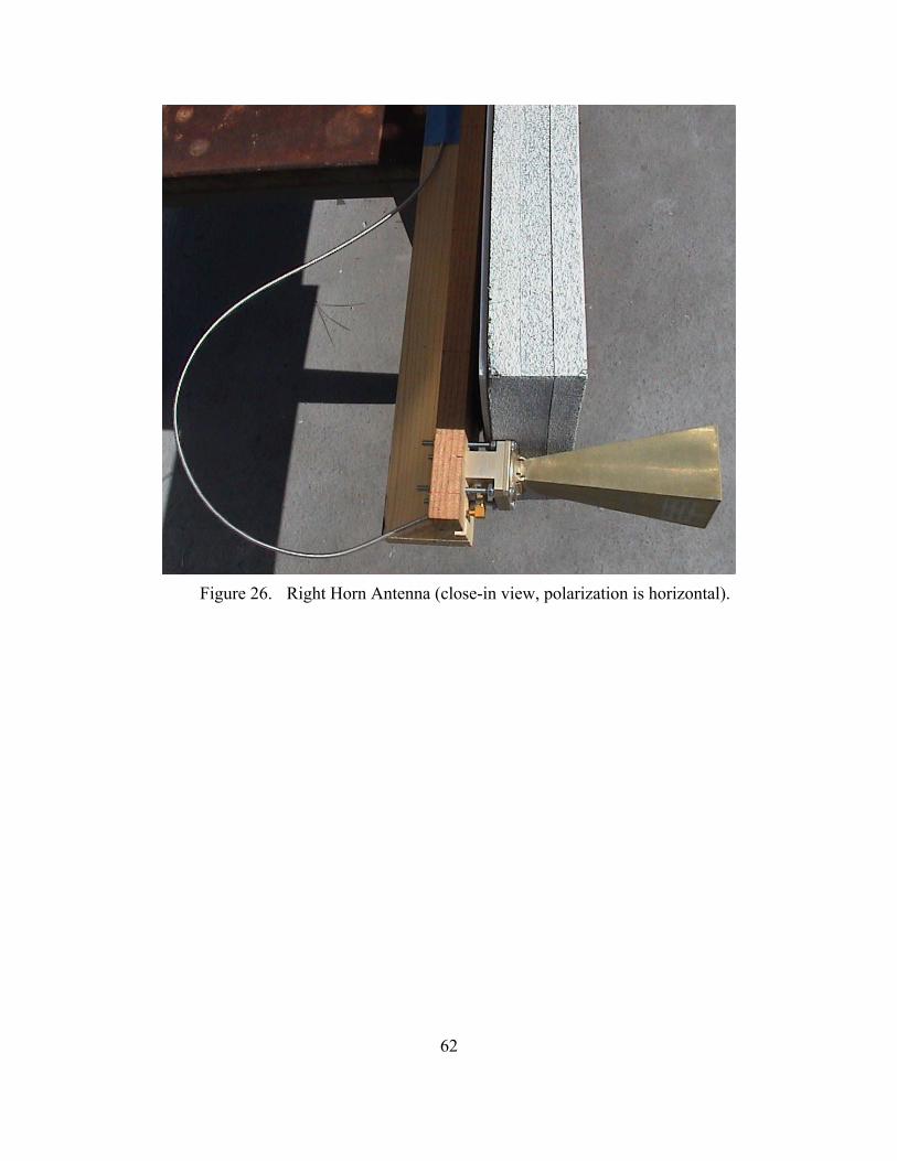
62
Figure 26. Right Horn Antenna (close-in view, polarization is horizontal).
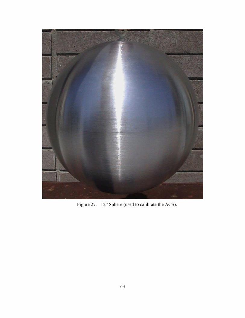
63
Figure 27. 12” Sphere (used to calibrate the ACS).

64
THIS PAGE INTENTIONALLY LEFT BLANK
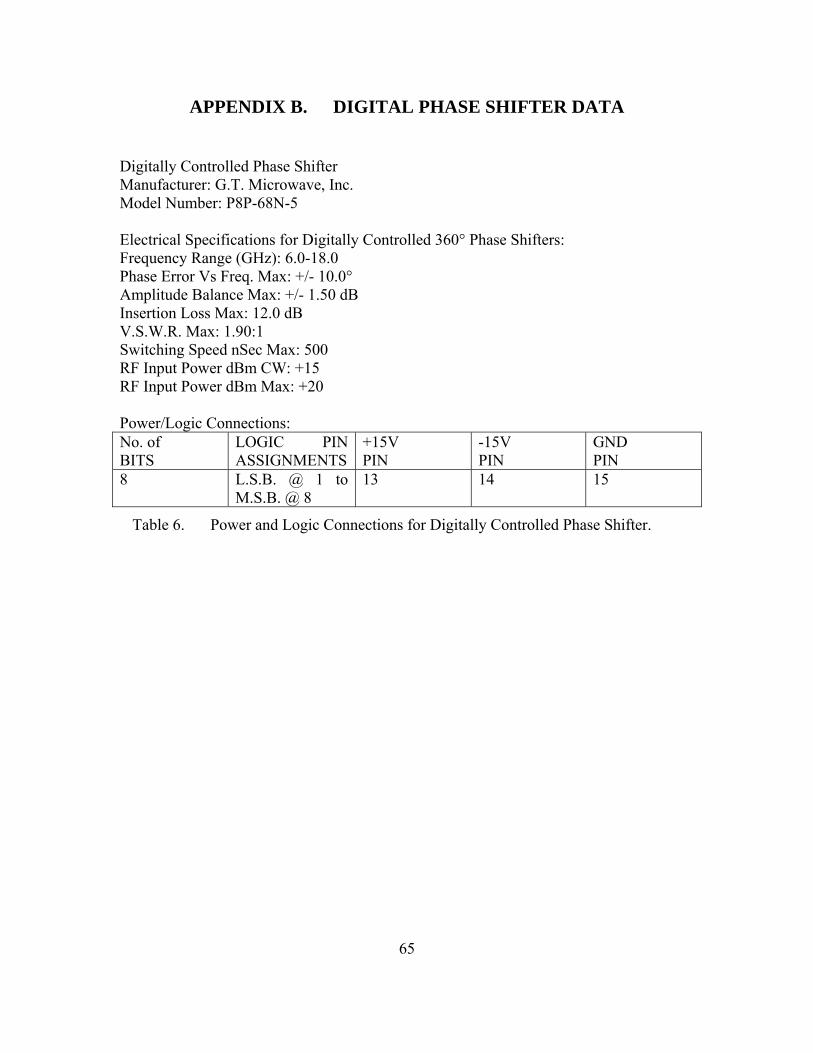
65
APPENDIX B. DIGITAL PHASE SHIFTER DATA
Digitally Controlled Phase Shifter Manufacturer: G.T. Microwave, Inc. Model Number: P8P-68N-5 Electrical Specifications for Digitally Controlled 360° Phase Shifters: Frequency Range (GHz): 6.0-18.0 Phase Error Vs Freq. Max: +/- 10.0° Amplitude Balance Max: +/- 1.50 dB Insertion Loss Max: 12.0 dB V.S.W.R. Max: 1.90:1 Switching Speed nSec Max: 500 RF Input Power dBm CW: +15 RF Input Power dBm Max: +20 Power/Logic Connections: No. of BITS
LOGIC PIN ASSIGNMENTS
+15V PIN
-15V PIN
GND PIN
8 L.S.B. @ 1 to M.S.B. @ 8
13 14 15
Table 6. Power and Logic Connections for Digitally Controlled Phase Shifter.
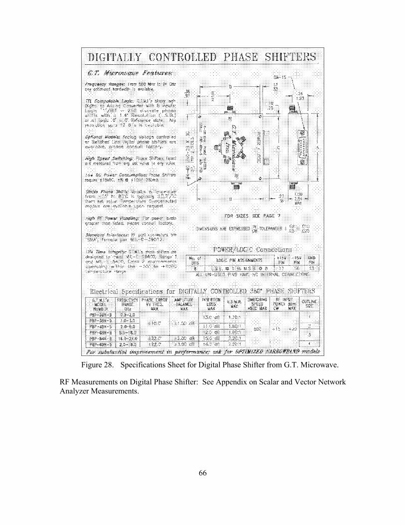
66
Figure 28. Specifications Sheet for Digital Phase Shifter from G.T. Microwave.
RF Measurements on Digital Phase Shifter: See Appendix on Scalar and Vector Network Analyzer Measurements.
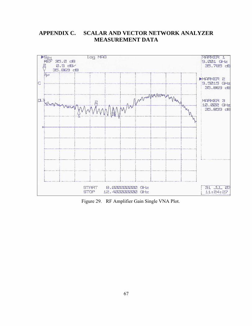
67
APPENDIX C. SCALAR AND VECTOR NETWORK ANALYZER MEASUREMENT DATA
Figure 29. RF Amplifier Gain Single VNA Plot.
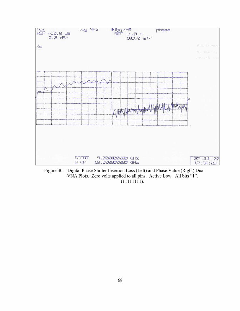
68
Figure 30. Digital Phase Shifter Insertion Loss (Left) and Phase Value (Right) Dual
VNA Plots. Zero volts applied to all pins. Active Low. All bits “1”. (11111111).
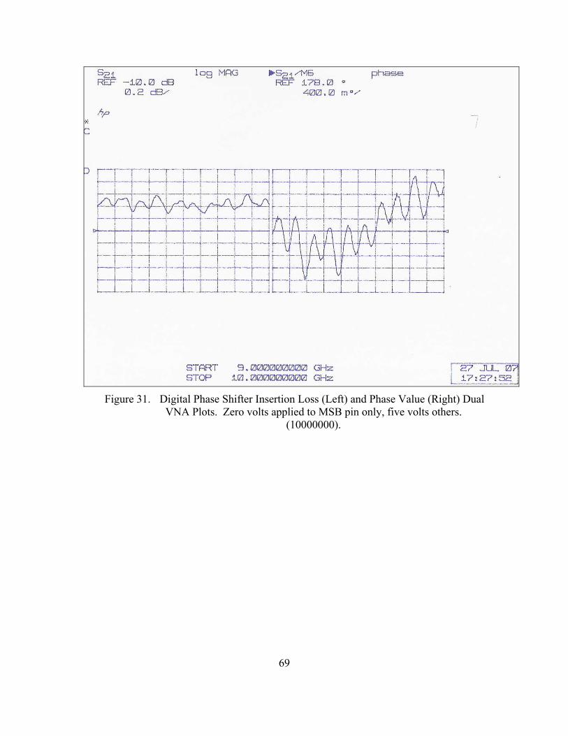
69
Figure 31. Digital Phase Shifter Insertion Loss (Left) and Phase Value (Right) Dual
VNA Plots. Zero volts applied to MSB pin only, five volts others. (10000000).
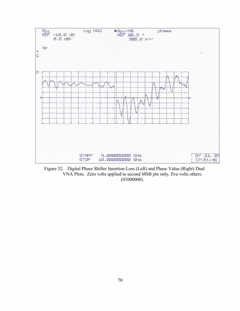
70
Figure 32. Digital Phase Shifter Insertion Loss (Left) and Phase Value (Right) Dual
VNA Plots. Zero volts applied to second MSB pin only, five volts others. (01000000).
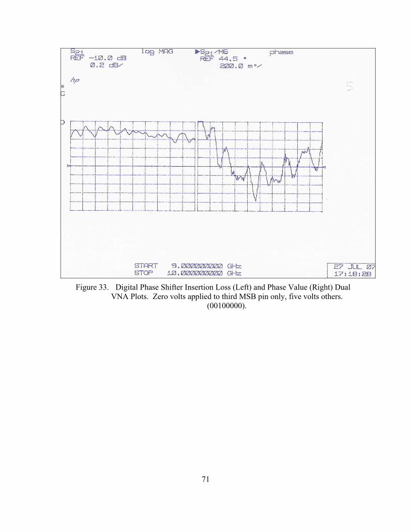
71
Figure 33. Digital Phase Shifter Insertion Loss (Left) and Phase Value (Right) Dual
VNA Plots. Zero volts applied to third MSB pin only, five volts others. (00100000).
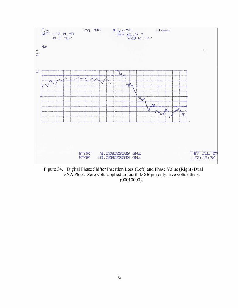
72
Figure 34. Digital Phase Shifter Insertion Loss (Left) and Phase Value (Right) Dual
VNA Plots. Zero volts applied to fourth MSB pin only, five volts others. (00010000).
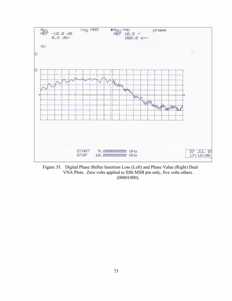
73
Figure 35. Digital Phase Shifter Insertion Loss (Left) and Phase Value (Right) Dual
VNA Plots. Zero volts applied to fifth MSB pin only, five volts others. (00001000).
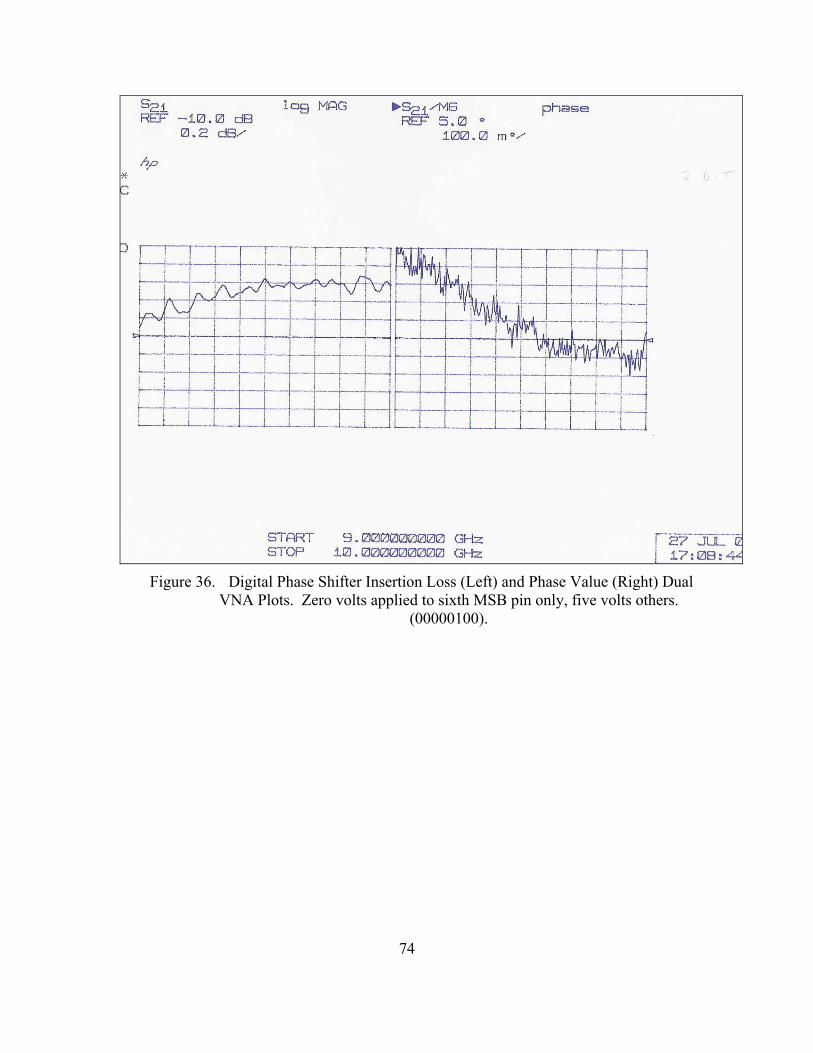
74
Figure 36. Digital Phase Shifter Insertion Loss (Left) and Phase Value (Right) Dual
VNA Plots. Zero volts applied to sixth MSB pin only, five volts others. (00000100).
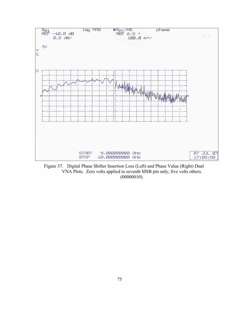
75
Figure 37. Digital Phase Shifter Insertion Loss (Left) and Phase Value (Right) Dual
VNA Plots. Zero volts applied to seventh MSB pin only, five volts others. (00000010).
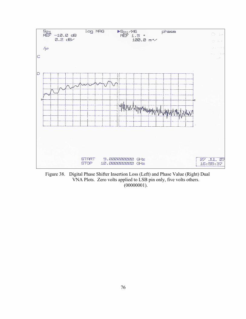
76
Figure 38. Digital Phase Shifter Insertion Loss (Left) and Phase Value (Right) Dual
VNA Plots. Zero volts applied to LSB pin only, five volts others. (00000001).
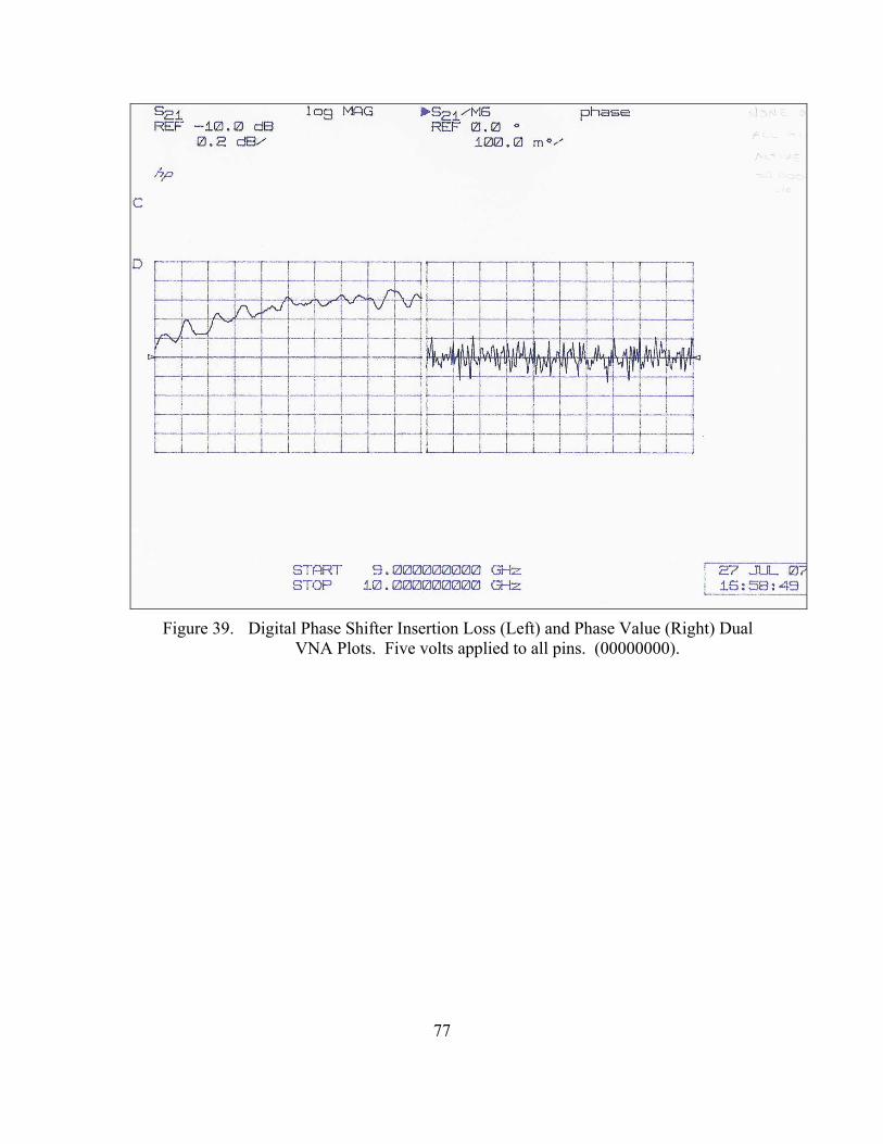
77
Figure 39. Digital Phase Shifter Insertion Loss (Left) and Phase Value (Right) Dual
VNA Plots. Five volts applied to all pins. (00000000).
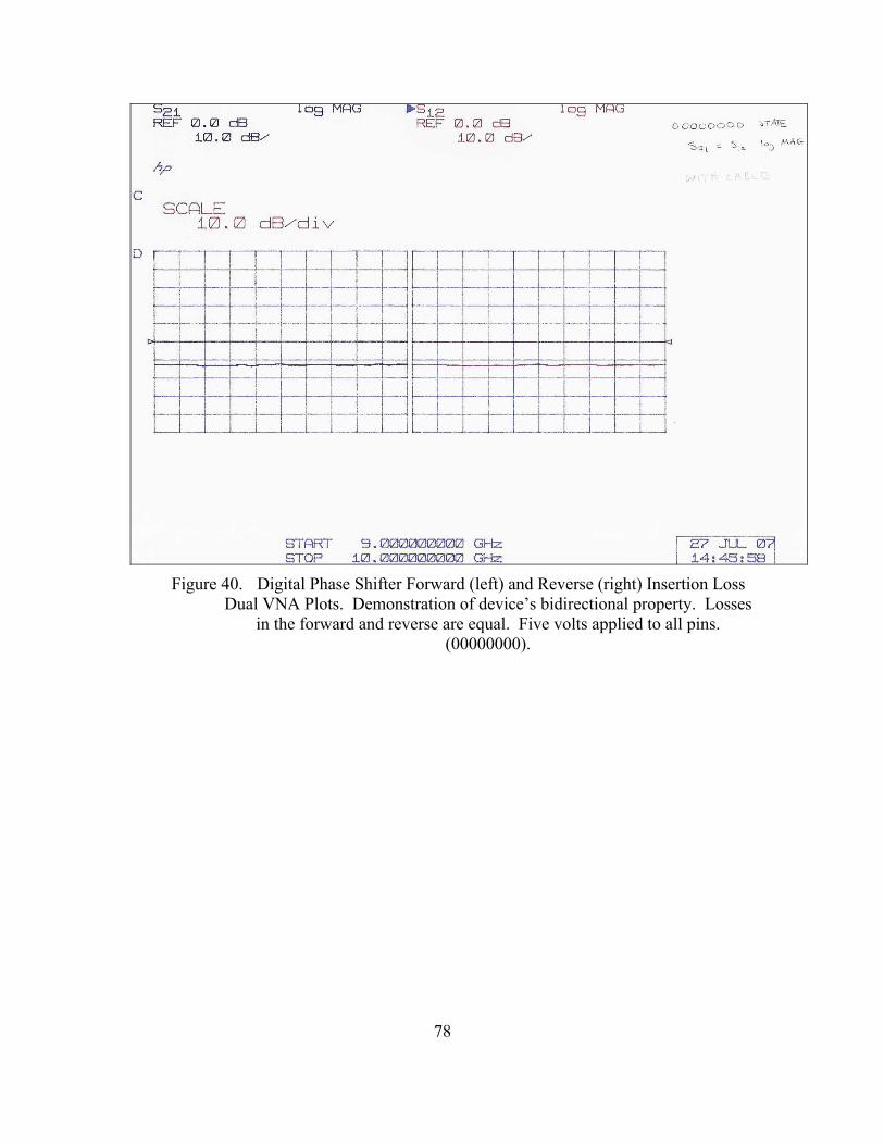
78
Figure 40. Digital Phase Shifter Forward (left) and Reverse (right) Insertion Loss
Dual VNA Plots. Demonstration of device’s bidirectional property. Losses in the forward and reverse are equal. Five volts applied to all pins.
(00000000).
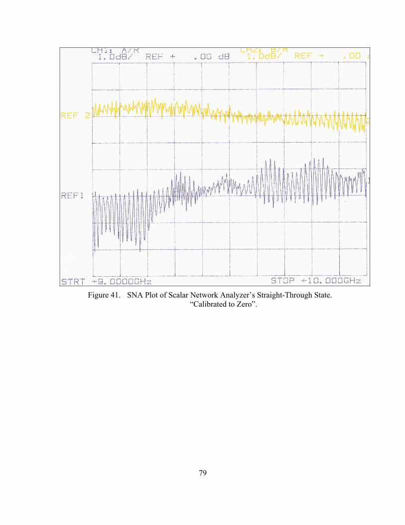
79
Figure 41. SNA Plot of Scalar Network Analyzer’s Straight-Through State.
“Calibrated to Zero”.
80
Figure 42. SNA Plot of Cable used with Digital Phase Shifter during SNA testing.
81
Figure 43. Digital Phase Shifter SNA Plot. Fixed Phase State, no Doppler Shift.
82
Figure 44. Digital Phase Shifter SNA Plot. Periodic Rotation through Phase States,
Doppler Shift.
83
Figure 45. Digital Phase Shifter Phase Value Single VNA Plot. Zero volts applied
to MSB pin only, five volts others. (10000000) 180° Phase Shift.
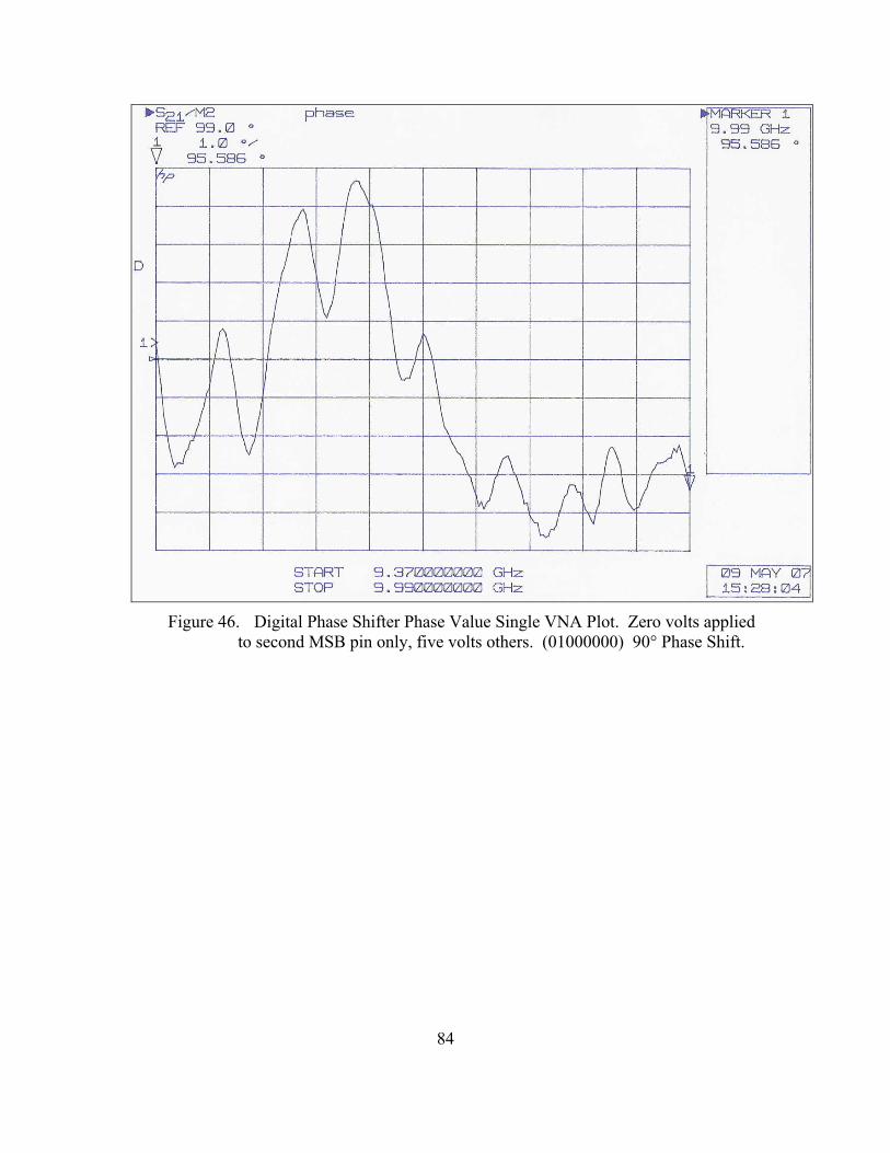
84
Figure 46. Digital Phase Shifter Phase Value Single VNA Plot. Zero volts applied
to second MSB pin only, five volts others. (01000000) 90° Phase Shift.
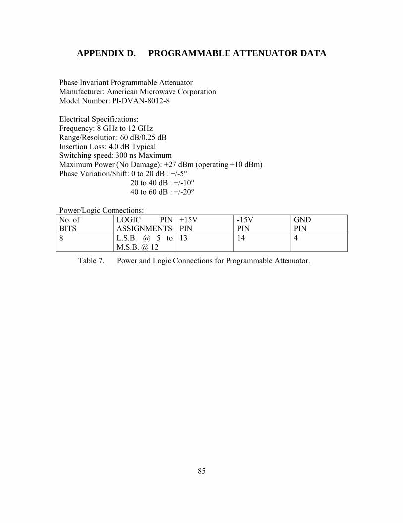
85
APPENDIX D. PROGRAMMABLE ATTENUATOR DATA
Phase Invariant Programmable Attenuator Manufacturer: American Microwave Corporation Model Number: PI-DVAN-8012-8 Electrical Specifications: Frequency: 8 GHz to 12 GHz Range/Resolution: 60 dB/0.25 dB Insertion Loss: 4.0 dB Typical Switching speed: 300 ns Maximum Maximum Power (No Damage): +27 dBm (operating +10 dBm) Phase Variation/Shift: 0 to 20 dB : +/-5°
20 to 40 dB : +/-10° 40 to 60 dB : +/-20°
Power/Logic Connections: No. of BITS
LOGIC PIN ASSIGNMENTS
+15V PIN
-15V PIN
GND PIN
8 L.S.B. @ 5 to M.S.B. @ 12
13 14 4
Table 7. Power and Logic Connections for Programmable Attenuator.
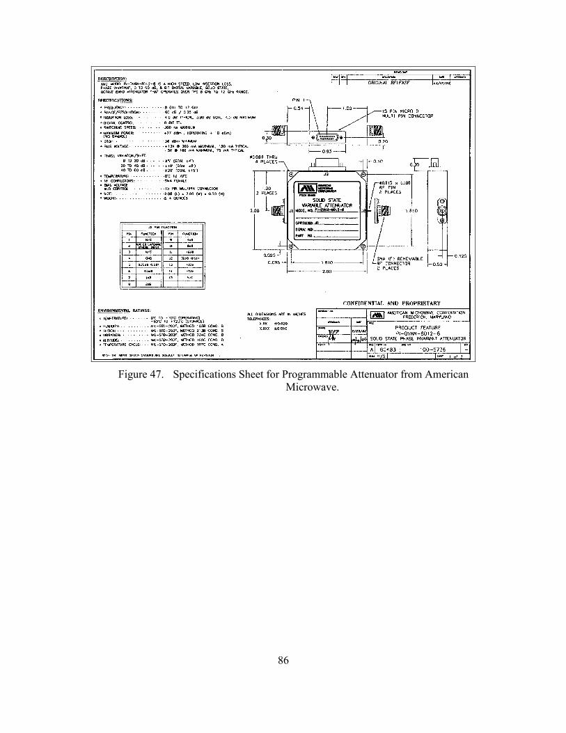
86
Figure 47. Specifications Sheet for Programmable Attenuator from American
Microwave.

87
APPENDIX E. ANTENNA DATA
Antenna List: (2) Pasternack Sectoral Horn Antennas (used as part of ACS) (2) Unknown X-band Quad-Ridge Dual-Pol Horn Antennas (used as part of anechoic chamber ACS testing) (1) Narda Standard Gain Horn Antenna (used as part of anechoic chamber antenna testing)
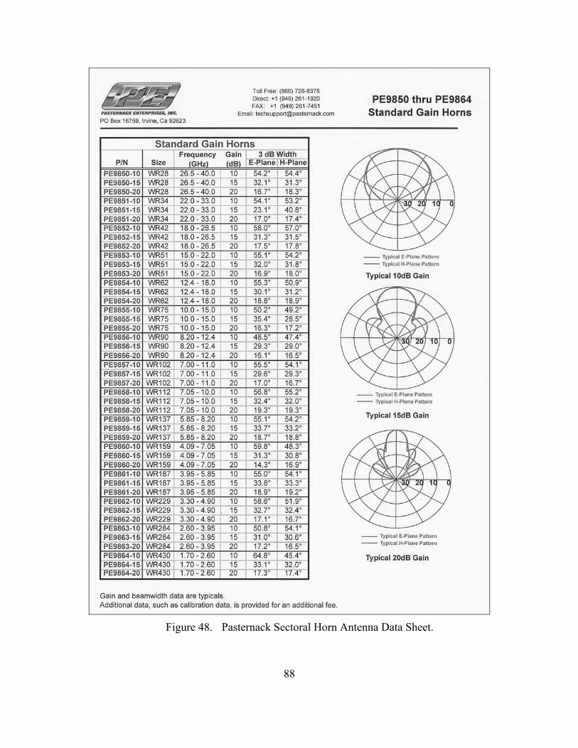
88
Figure 48. Pasternack Sectoral Horn Antenna Data Sheet.
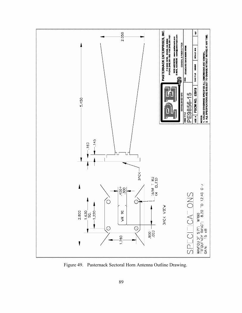
89
Figure 49. Pasternack Sectoral Horn Antenna Outline Drawing.
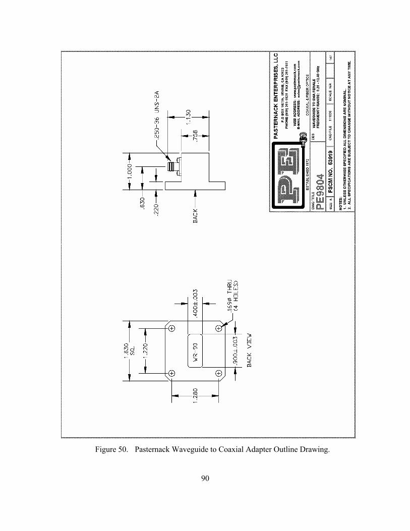
90
Figure 50. Pasternack Waveguide to Coaxial Adapter Outline Drawing.
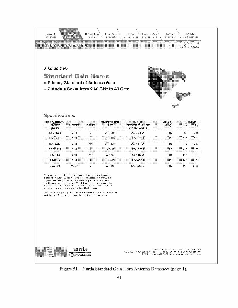
91
Figure 51. Narda Standard Gain Horn Antenna Datasheet (page 1).
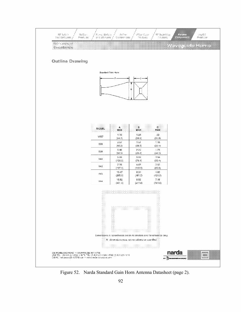
92
Figure 52. Narda Standard Gain Horn Antenna Datasheet (page 2).
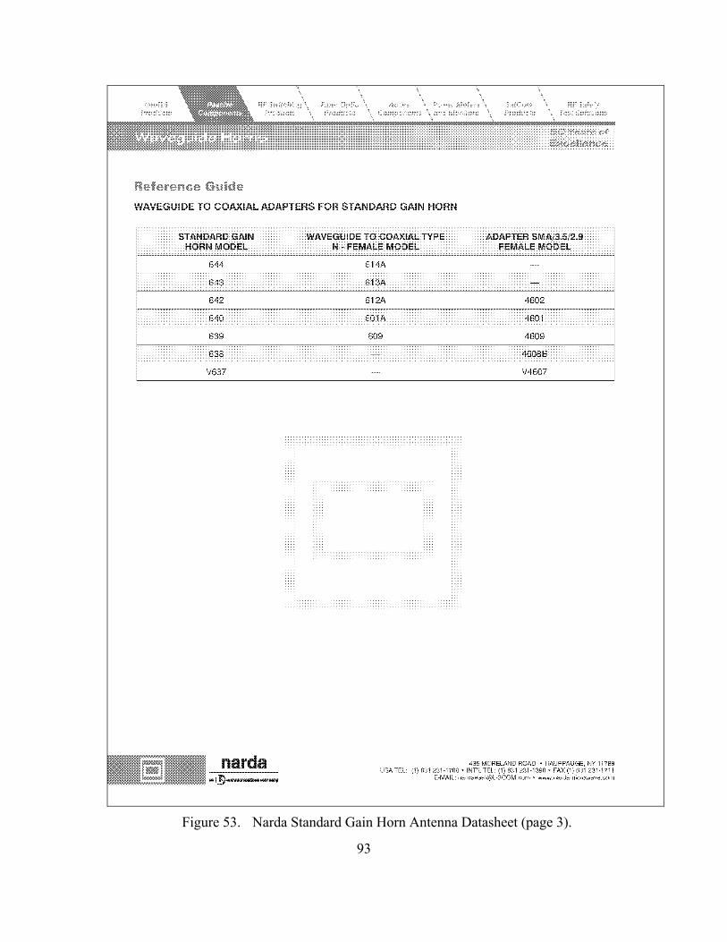
93
Figure 53. Narda Standard Gain Horn Antenna Datasheet (page 3).
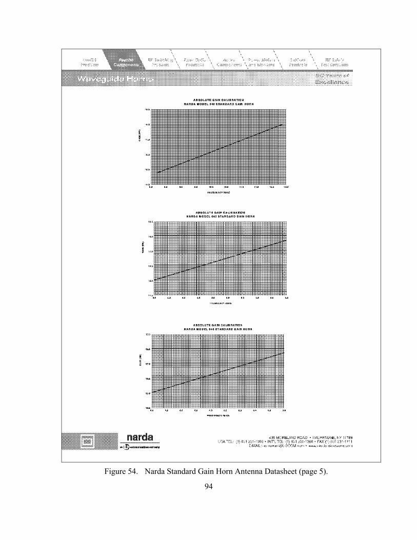
94
Figure 54. Narda Standard Gain Horn Antenna Datasheet (page 5).
95
APPENDIX F. ANTENNA PATTERN DATA
A total of five antennas were used in testing. One Narda standard gain horn
antenna was used during antenna testing (patterns) only. Two X-band horn antennas
were used during antenna testing (patterns), then used during ACS testing (as the transmit
and receive antennas of the radar/VNA). Two Pasternack horn antennas were used
during antenna testing (patterns), then used during ACS testing (as the transmit and
receive antennas of the ACS). Measurements were made at three frequencies: 9370,
9680, and 9990 MHz (low, mid, and high frequency points on the MWR-05XP weather
radar’s RF band). E-plane and H-plane patterns were measured. To measure both
planes, the antenna under test was first rotated 360° in azimuth with the radiator oriented
for horizontal polarization (E-plane), then rolled 90° and the process repeated with the
radiator now oriented for vertical polarization (H-plane). In total, two plane patterns
were measured for five antennas at three frequencies to create thirty data sets.
A. VNA ANTENNA PATTERN DATA
In all plots, solid line is for X-band Horn Antenna #1 (“xbh”) and dotted line is
for X-band Horn Antenna #2 (“ybh”). The last three plots are solid line for the Standard
Gain Horn (“sgh”) which are included to provide a gain reference.
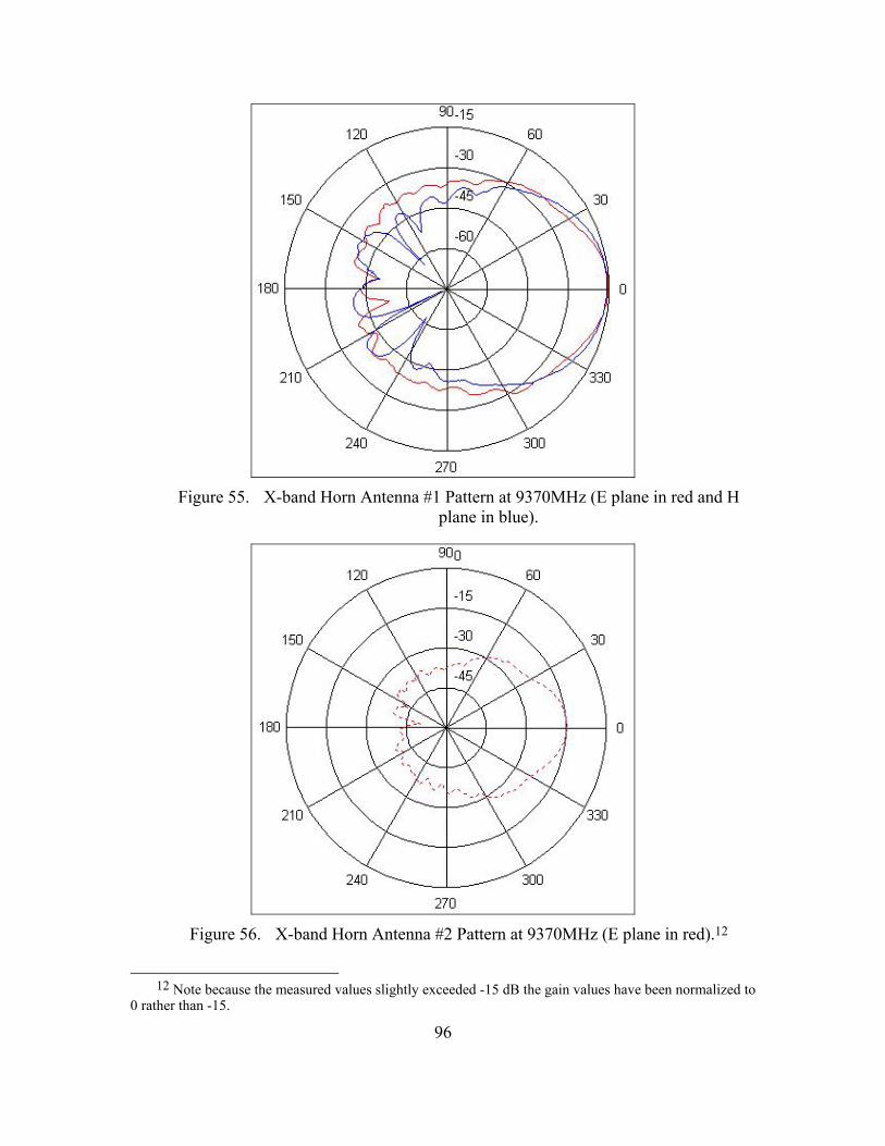
96
Figure 55. X-band Horn Antenna #1 Pattern at 9370MHz (E plane in red and H
plane in blue).
Figure 56. X-band Horn Antenna #2 Pattern at 9370MHz (E plane in red).12
12 Note because the measured values slightly exceeded -15 dB the gain values have been normalized to
0 rather than -15.
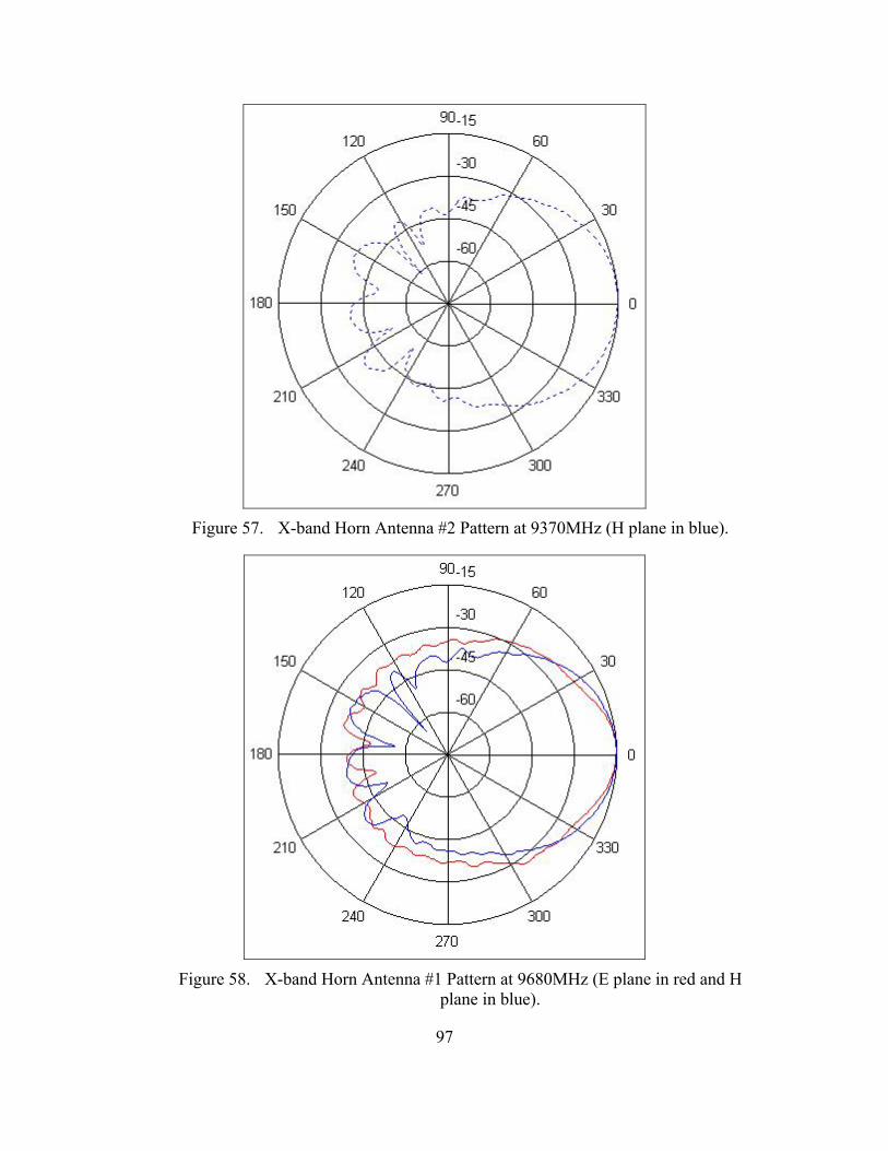
97
Figure 57. X-band Horn Antenna #2 Pattern at 9370MHz (H plane in blue).
Figure 58. X-band Horn Antenna #1 Pattern at 9680MHz (E plane in red and H
plane in blue).
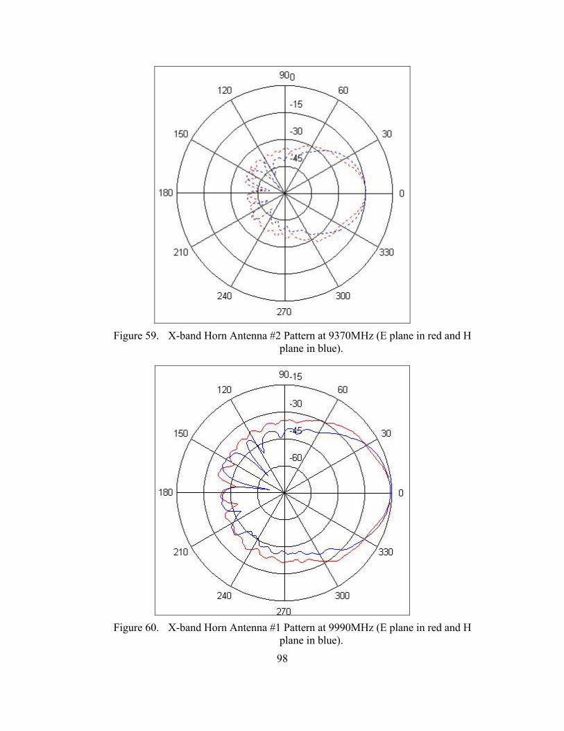
98
Figure 59. X-band Horn Antenna #2 Pattern at 9370MHz (E plane in red and H
plane in blue).
Figure 60. X-band Horn Antenna #1 Pattern at 9990MHz (E plane in red and H
plane in blue).
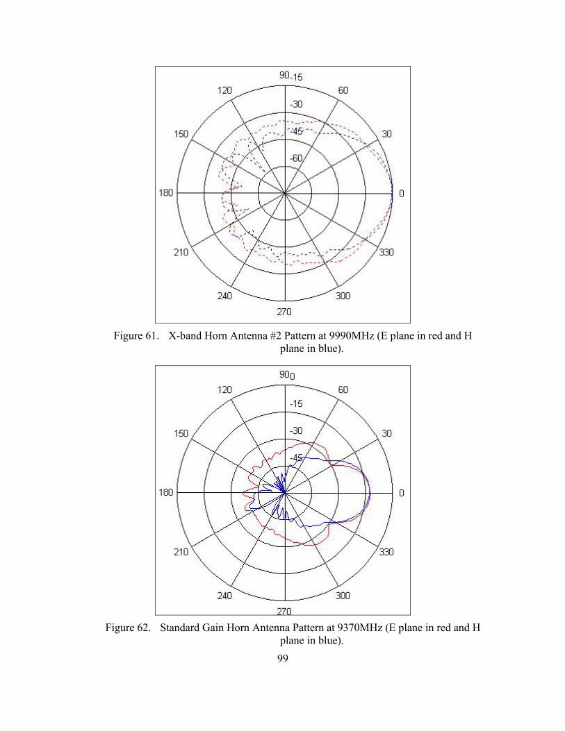
99
Figure 61. X-band Horn Antenna #2 Pattern at 9990MHz (E plane in red and H
plane in blue).
Figure 62. Standard Gain Horn Antenna Pattern at 9370MHz (E plane in red and H
plane in blue).
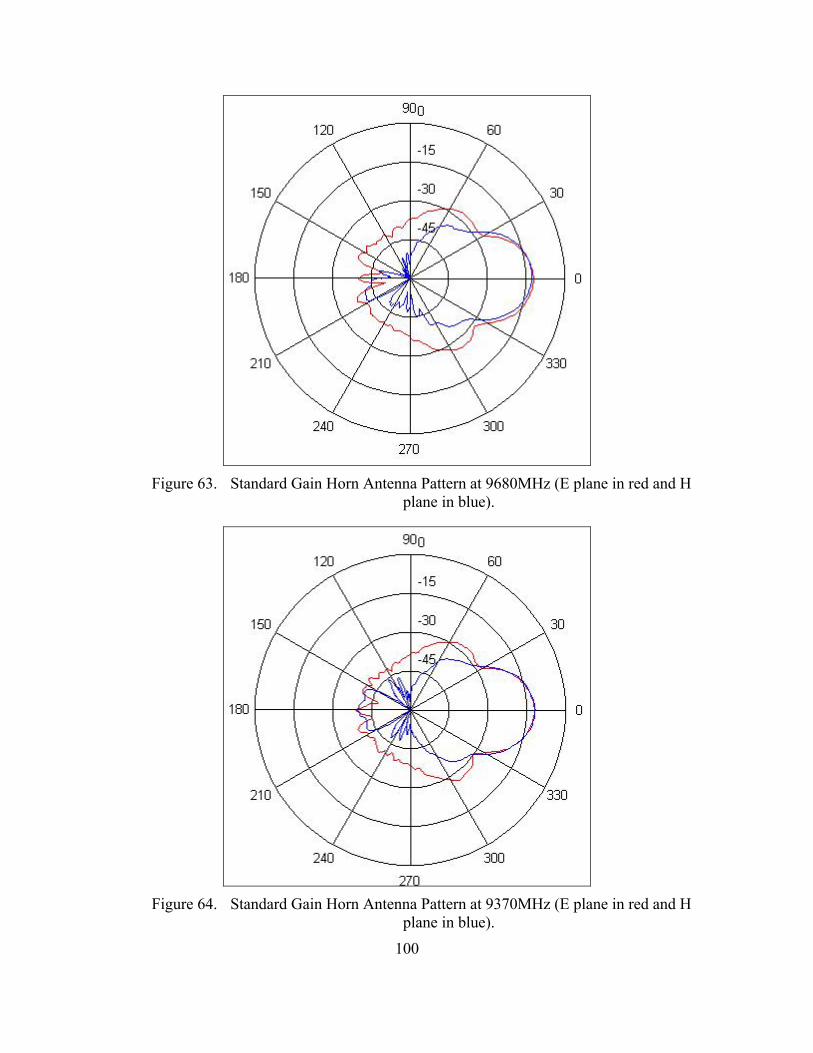
100
Figure 63. Standard Gain Horn Antenna Pattern at 9680MHz (E plane in red and H
plane in blue).
Figure 64. Standard Gain Horn Antenna Pattern at 9370MHz (E plane in red and H
plane in blue).
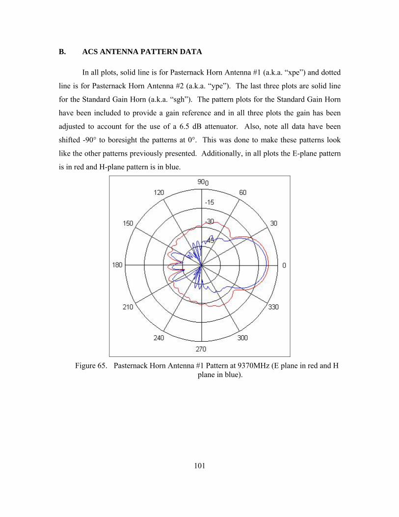
101
B. ACS ANTENNA PATTERN DATA
In all plots, solid line is for Pasternack Horn Antenna #1 (a.k.a. “xpe”) and dotted
line is for Pasternack Horn Antenna #2 (a.k.a. “ype”). The last three plots are solid line
for the Standard Gain Horn (a.k.a. “sgh”). The pattern plots for the Standard Gain Horn
have been included to provide a gain reference and in all three plots the gain has been
adjusted to account for the use of a 6.5 dB attenuator. Also, note all data have been
shifted -90° to boresight the patterns at 0°. This was done to make these patterns look
like the other patterns previously presented. Additionally, in all plots the E-plane pattern
is in red and H-plane pattern is in blue.
Figure 65. Pasternack Horn Antenna #1 Pattern at 9370MHz (E plane in red and H
plane in blue).
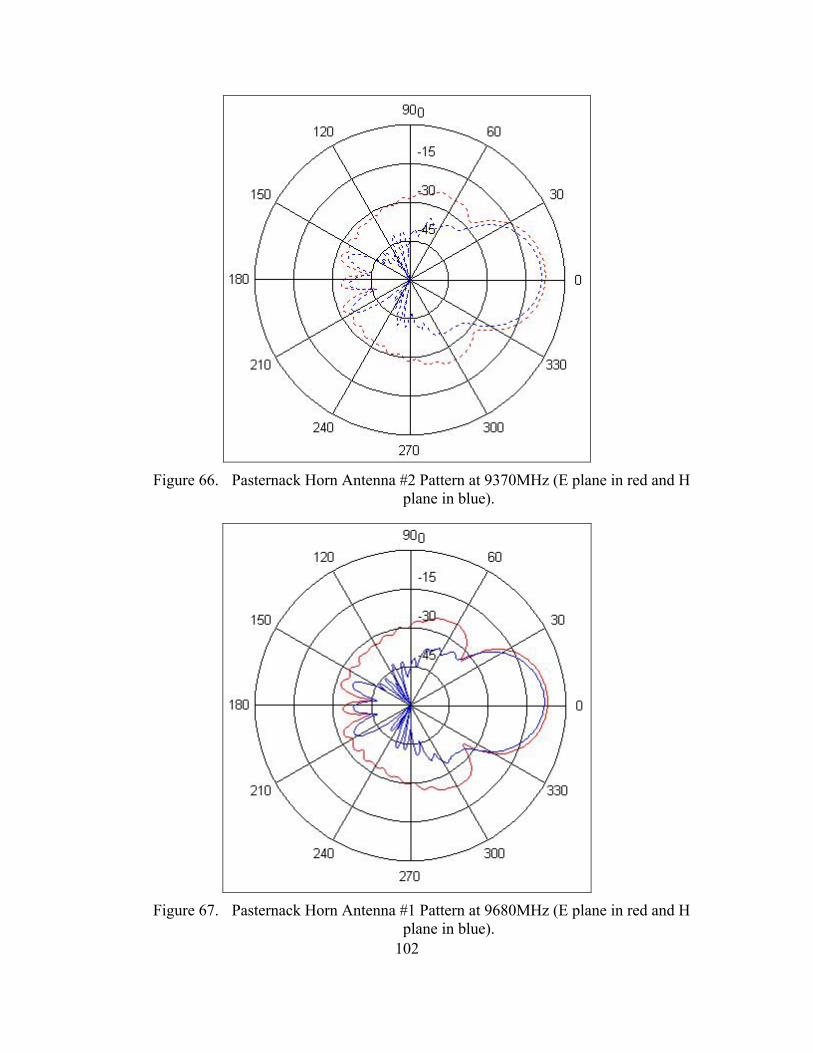
102
Figure 66. Pasternack Horn Antenna #2 Pattern at 9370MHz (E plane in red and H
plane in blue).
Figure 67. Pasternack Horn Antenna #1 Pattern at 9680MHz (E plane in red and H
plane in blue).
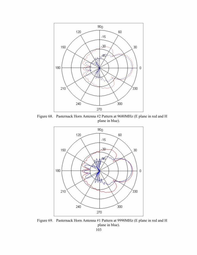
103
Figure 68. Pasternack Horn Antenna #2 Pattern at 9680MHz (E plane in red and H
plane in blue).
Figure 69. Pasternack Horn Antenna #1 Pattern at 9990MHz (E plane in red and H
plane in blue).
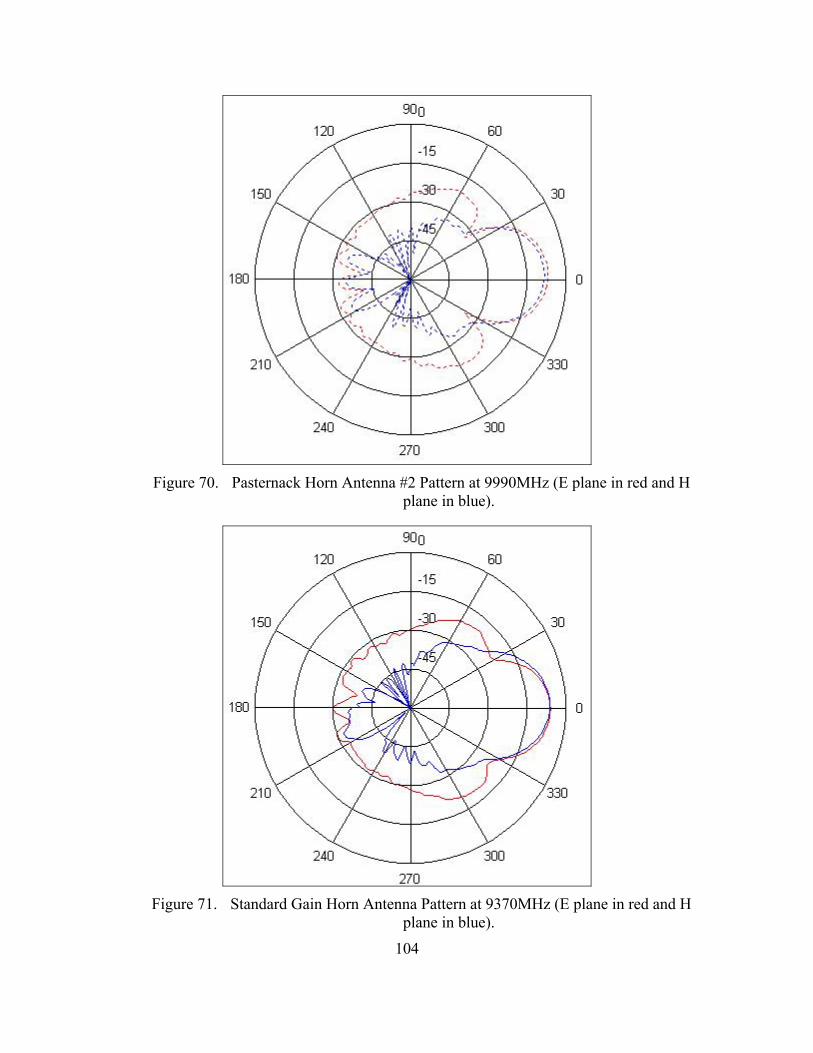
104
Figure 70. Pasternack Horn Antenna #2 Pattern at 9990MHz (E plane in red and H
plane in blue).
Figure 71. Standard Gain Horn Antenna Pattern at 9370MHz (E plane in red and H
plane in blue).
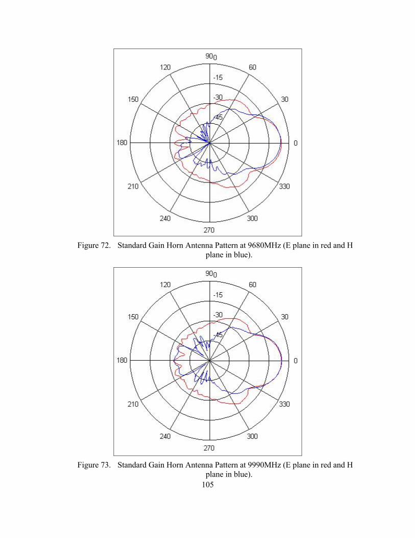
105
Figure 72. Standard Gain Horn Antenna Pattern at 9680MHz (E plane in red and H
plane in blue).
Figure 73. Standard Gain Horn Antenna Pattern at 9990MHz (E plane in red and H
plane in blue).
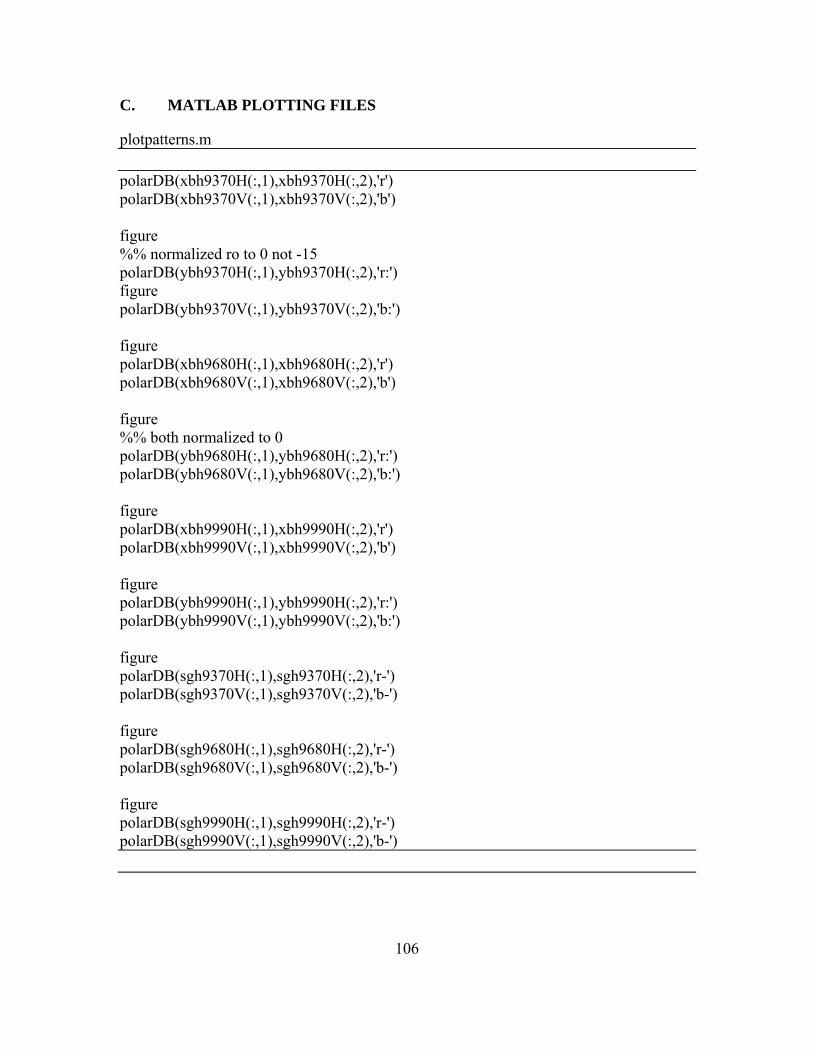
106
C. MATLAB PLOTTING FILES
plotpatterns.m polarDB(xbh9370H(:,1),xbh9370H(:,2),'r') polarDB(xbh9370V(:,1),xbh9370V(:,2),'b') figure %% normalized ro to 0 not -15 polarDB(ybh9370H(:,1),ybh9370H(:,2),'r:') figure polarDB(ybh9370V(:,1),ybh9370V(:,2),'b:') figure polarDB(xbh9680H(:,1),xbh9680H(:,2),'r') polarDB(xbh9680V(:,1),xbh9680V(:,2),'b') figure %% both normalized to 0 polarDB(ybh9680H(:,1),ybh9680H(:,2),'r:') polarDB(ybh9680V(:,1),ybh9680V(:,2),'b:') figure polarDB(xbh9990H(:,1),xbh9990H(:,2),'r') polarDB(xbh9990V(:,1),xbh9990V(:,2),'b') figure polarDB(ybh9990H(:,1),ybh9990H(:,2),'r:') polarDB(ybh9990V(:,1),ybh9990V(:,2),'b:') figure polarDB(sgh9370H(:,1),sgh9370H(:,2),'r-') polarDB(sgh9370V(:,1),sgh9370V(:,2),'b-') figure polarDB(sgh9680H(:,1),sgh9680H(:,2),'r-') polarDB(sgh9680V(:,1),sgh9680V(:,2),'b-') figure polarDB(sgh9990H(:,1),sgh9990H(:,2),'r-') polarDB(sgh9990V(:,1),sgh9990V(:,2),'b-')
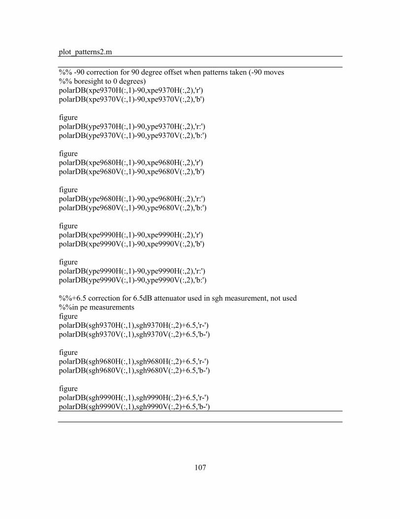
107
plot_patterns2.m %% -90 correction for 90 degree offset when patterns taken (-90 moves %% boresight to 0 degrees) polarDB(xpe9370H(:,1)-90,xpe9370H(:,2),'r') polarDB(xpe9370V(:,1)-90,xpe9370V(:,2),'b') figure polarDB(ype9370H(:,1)-90,ype9370H(:,2),'r:') polarDB(ype9370V(:,1)-90,ype9370V(:,2),'b:') figure polarDB(xpe9680H(:,1)-90,xpe9680H(:,2),'r') polarDB(xpe9680V(:,1)-90,xpe9680V(:,2),'b') figure polarDB(ype9680H(:,1)-90,ype9680H(:,2),'r:') polarDB(ype9680V(:,1)-90,ype9680V(:,2),'b:') figure polarDB(xpe9990H(:,1)-90,xpe9990H(:,2),'r') polarDB(xpe9990V(:,1)-90,xpe9990V(:,2),'b') figure polarDB(ype9990H(:,1)-90,ype9990H(:,2),'r:') polarDB(ype9990V(:,1)-90,ype9990V(:,2),'b:') %%+6.5 correction for 6.5dB attenuator used in sgh measurement, not used %%in pe measurements figure polarDB(sgh9370H(:,1),sgh9370H(:,2)+6.5,'r-') polarDB(sgh9370V(:,1),sgh9370V(:,2)+6.5,'b-') figure polarDB(sgh9680H(:,1),sgh9680H(:,2)+6.5,'r-') polarDB(sgh9680V(:,1),sgh9680V(:,2)+6.5,'b-') figure polarDB(sgh9990H(:,1),sgh9990H(:,2)+6.5,'r-') polarDB(sgh9990V(:,1),sgh9990V(:,2)+6.5,'b-')
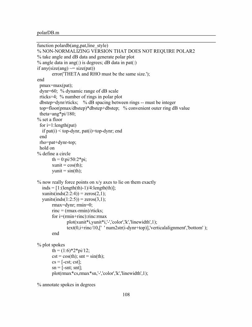
108
polarDB.m function polardb(ang,pat,line_style) % NON-NORMALIZING VERSION THAT DOES NOT REQUIRE POLAR2 % take angle and dB data and generate polar plot % angle data in ang(:) is degrees; dB data in pat(:) if any(size(ang) ~= size(pat)) error('THETA and RHO must be the same size.'); end pmax=max(pat); dynr=60; % dynamic range of dB scale rticks=4; % number of rings in polar plot dbstep=dynr/rticks; % dB spacing between rings -- must be integer top=floor(pmax/dbstep)*dbstep+dbstep; % convenient outer ring dB value theta=ang*pi/180; % set a floor for i=1:length(pat) if pat(i) < top-dynr, pat(i)=top-dynr; end end rho=pat+dynr-top; hold on % define a circle th = 0:pi/50:2*pi; xunit = cos(th); yunit = sin(th); % now really force points on x/y axes to lie on them exactly inds = [1:(length(th)-1)/4:length(th)]; xunits(inds(2:2:4)) = zeros(2,1); yunits(inds(1:2:5)) = zeros(3,1); rmax=dynr; rmin=0; rinc = (rmax-rmin)/rticks; for i=(rmin+rinc):rinc:rmax plot(xunit*i,yunit*i,'-','color','k','linewidth',1); text(0,i+rinc/10,[' ' num2str(i-dynr+top)],'verticalalignment','bottom' ); end % plot spokes th = (1:6)*2*pi/12; cst = cos(th); snt = sin(th); cs = [-cst; cst]; sn = [-snt; snt]; plot(rmax*cs,rmax*sn,'-','color','k','linewidth',1); % annotate spokes in degrees
109
rt = 1.1*rmax; for i = 1:max(size(th)) text(rt*cst(i),rt*snt(i),int2str(i*30),'horizontalalignment','center' ); if i == max(size(th)) loc = int2str(0); else loc = int2str(180+i*30); end text(-rt*cst(i),-rt*snt(i),loc,'horizontalalignment','center' ); end % set viewto 2-D view(0,90); % set axis limits axis(rmax*[-1 1 -1.1 1.1]); % transform data to Cartesian coordinates xx = rho.*cos(theta); yy = rho.*sin(theta); % plot data on top of grid q = plot(xx,yy,line_style); hpol = q; axis('equal');axis('off'); hold off
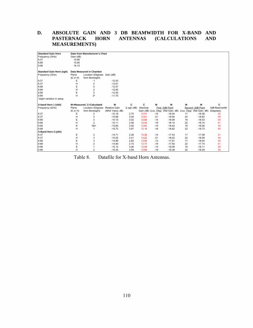
110
D. ABSOLUTE GAIN AND 3 DB BEAMWIDTH FOR X-BAND AND PASTERNACK HORN ANTENNAS (CALCULATIONS AND MEASUREMENTS)
Standard Gain Horn Data from Manufacturer's ChartFrequency (GHz) Gain (dB)9.37 15.669.68 15.909.99 16.15
Standard Gain Horn (sgh) Data Measured in ChamberFrequency (GHz) Plane
(E or H)Location (Degreesfrom Boresight)
Gain (dB)
9.37 E -1 -12.439.37 H 2 -12.619.68 E 0 -12.079.68 H 2 -12.659.99 E 0 -12.059.99 H 0* -11.75*slight variation in setup
X-band Horn 1 (xbh) M=Measured, C=Calculated M C C M M M M CFrequency (GHz) Δ sgh (dB) 3dB Beamwidth
(Loc, Deg) (Rel Gain, dB) (Loc, Deg) (Rel Gain, dB) (Degrees)9.37 E 2 -15.18 2.75 12.91 -15 -18.04 17 -18.08 329.37 H 3 -15.66 3.04 12.61 -21 -18.64 24 -18.62 459.68 E 3 -15.10 3.02 12.88 -14 -18.09 16 -18.03 309.68 H 2 -15.11 2.46 13.44 -19 -18.14 22 -18.10 419.99 E 0&1 -15.60 3.55 12.60 -14 -18.42 16 -18.56 309.99 H 1 -15.72 3.97 12.18 -18 -18.62 22 -18.73 40X-Band Horn 2 (ybh)9.37 E 2 -14.71 2.28 13.38 -14 -17.43 17 -17.58 319.37 H 3 -15.02 2.41 13.25 -21 -18.02 24 -18.06 459.68 E 3 -14.89 2.82 13.08 -13 -17.81 17 -18.04 309.68 H 2 -14.80 2.15 13.75 -19 -17.93 22 -17.74 419.99 E 1 -15.12 3.06 13.09 -14 -18.09 16 -18.11 309.99 H 2 -15.34 3.59 12.56 -18 -18.38 22 -18.29 40
Plane(E or H)
First -3dB Point Second -3dB PointLocation (Degreesfrom Boresight)
Relative Gain(MAX Value, dB)
AbsoluteGain (dB)
Table 8. Datafile for X-band Horn Antennas.
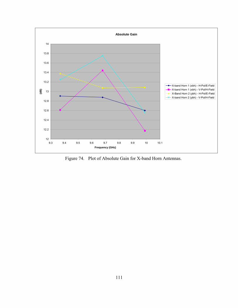
111
Absolute Gain
12
12.2
12.4
12.6
12.8
13
13.2
13.4
13.6
13.8
14
9.3 9.4 9.5 9.6 9.7 9.8 9.9 10 10.1
Frequency (GHz)
(dB
)
X-band Horn 1 (xbh) - H-Pol/E-FieldX-band Horn 1 (xbh) - V-Pol/H-FieldX-Band Horn 2 (ybh) - H-Pol/E-FieldX-band Horn 2 (ybh) - V-Pol/H-Field
Figure 74. Plot of Absolute Gain for X-band Horn Antennas.
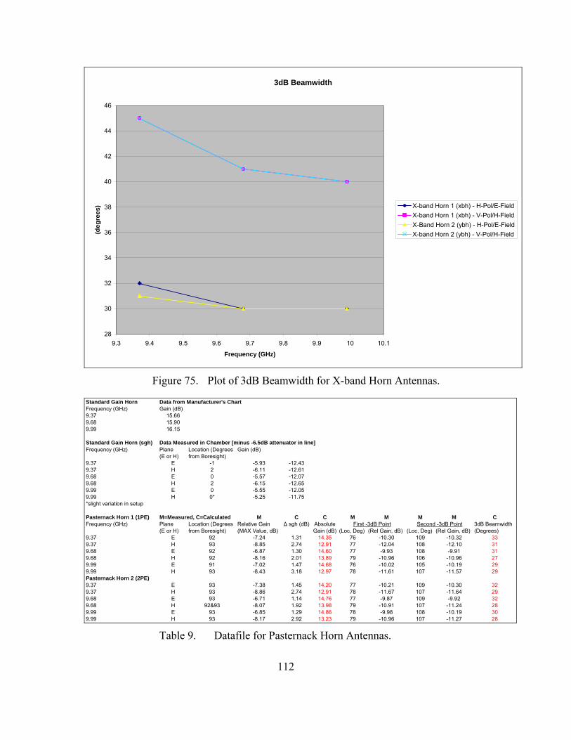
112
3dB Beamwidth
28
30
32
34
36
38
40
42
44
46
9.3 9.4 9.5 9.6 9.7 9.8 9.9 10 10.1
Frequency (GHz)
(deg
rees
) X-band Horn 1 (xbh) - H-Pol/E-FieldX-band Horn 1 (xbh) - V-Pol/H-FieldX-Band Horn 2 (ybh) - H-Pol/E-FieldX-band Horn 2 (ybh) - V-Pol/H-Field
Figure 75. Plot of 3dB Beamwidth for X-band Horn Antennas.
Standard Gain Horn Data from Manufacturer's ChartFrequency (GHz) Gain (dB)9.37 15.669.68 15.909.99 16.15
Standard Gain Horn (sgh) Data Measured in Chamber [minus -6.5dB attenuator in line]Frequency (GHz) Plane
(E or H)Location (Degreesfrom Boresight)
Gain (dB)
9.37 E -1 -5.93 -12.439.37 H 2 -6.11 -12.619.68 E 0 -5.57 -12.079.68 H 2 -6.15 -12.659.99 E 0 -5.55 -12.059.99 H 0* -5.25 -11.75*slight variation in setup
Pasternack Horn 1 (1PE) M=Measured, C=Calculated M C C M M M M CFrequency (GHz) Δ sgh (dB) 3dB Beamwidth
(Loc, Deg) (Rel Gain, dB) (Loc, Deg) (Rel Gain, dB) (Degrees)9.37 E 92 -7.24 1.31 14.35 76 -10.30 109 -10.32 339.37 H 93 -8.85 2.74 12.91 77 -12.04 108 -12.10 319.68 E 92 -6.87 1.30 14.60 77 -9.93 108 -9.91 319.68 H 92 -8.16 2.01 13.89 79 -10.96 106 -10.96 279.99 E 91 -7.02 1.47 14.68 76 -10.02 105 -10.19 299.99 H 93 -8.43 3.18 12.97 78 -11.61 107 -11.57 29Pasternack Horn 2 (2PE)9.37 E 93 -7.38 1.45 14.20 77 -10.21 109 -10.30 329.37 H 93 -8.86 2.74 12.91 78 -11.67 107 -11.64 299.68 E 93 -6.71 1.14 14.76 77 -9.87 109 -9.92 329.68 H 92&93 -8.07 1.92 13.98 79 -10.91 107 -11.24 289.99 E 93 -6.85 1.29 14.86 78 -9.98 108 -10.19 309.99 H 93 -8.17 2.92 13.23 79 -10.96 107 -11.27 28
First -3dB Point Second -3dB PointPlane(E or H)
Location (Degreesfrom Boresight)
Relative Gain(MAX Value, dB)
AbsoluteGain (dB)
Table 9. Datafile for Pasternack Horn Antennas.
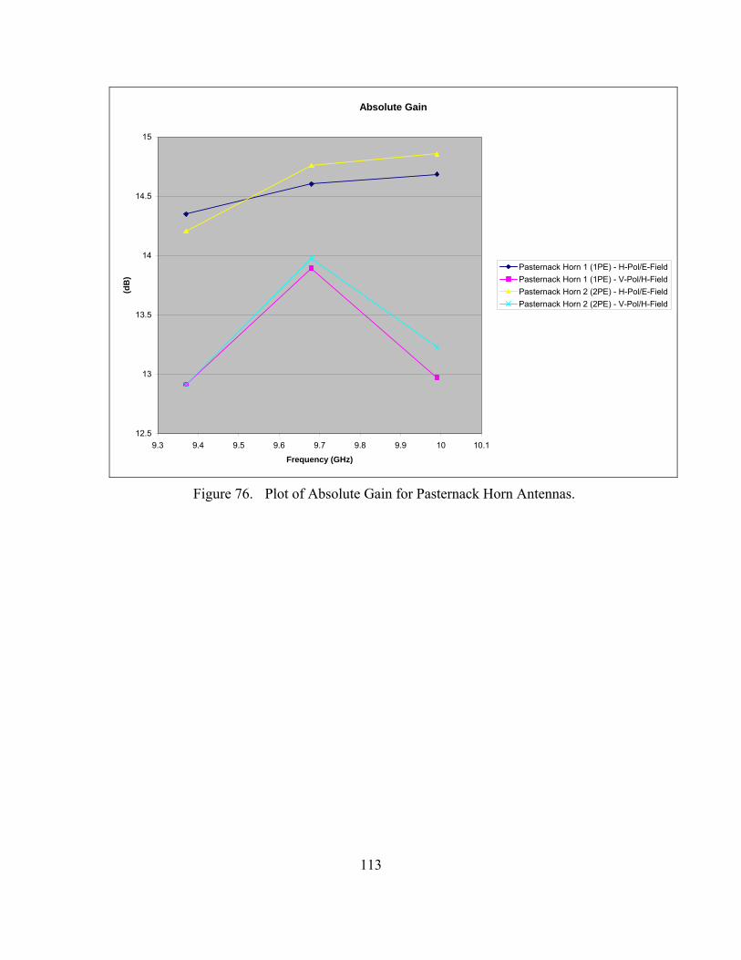
113
Absolute Gain
12.5
13
13.5
14
14.5
15
9.3 9.4 9.5 9.6 9.7 9.8 9.9 10 10.1
Frequency (GHz)
(dB
)
Pasternack Horn 1 (1PE) - H-Pol/E-FieldPasternack Horn 1 (1PE) - V-Pol/H-FieldPasternack Horn 2 (2PE) - H-Pol/E-FieldPasternack Horn 2 (2PE) - V-Pol/H-Field
Figure 76. Plot of Absolute Gain for Pasternack Horn Antennas.
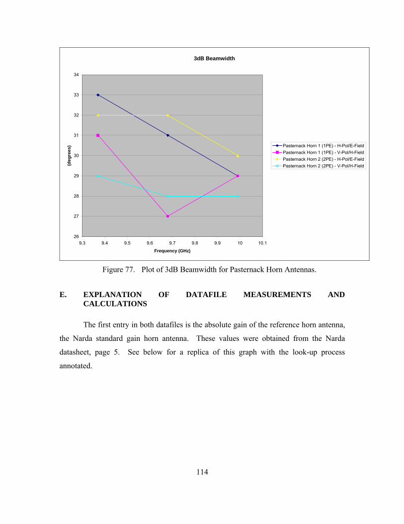
114
3dB Beamwidth
26
27
28
29
30
31
32
33
34
9.3 9.4 9.5 9.6 9.7 9.8 9.9 10 10.1
Frequency (GHz)
(deg
rees
) Pasternack Horn 1 (1PE) - H-Pol/E-FieldPasternack Horn 1 (1PE) - V-Pol/H-FieldPasternack Horn 2 (2PE) - H-Pol/E-FieldPasternack Horn 2 (2PE) - V-Pol/H-Field
Figure 77. Plot of 3dB Beamwidth for Pasternack Horn Antennas.
E. EXPLANATION OF DATAFILE MEASUREMENTS AND CALCULATIONS
The first entry in both datafiles is the absolute gain of the reference horn antenna,
the Narda standard gain horn antenna. These values were obtained from the Narda
datasheet, page 5. See below for a replica of this graph with the look-up process
annotated.
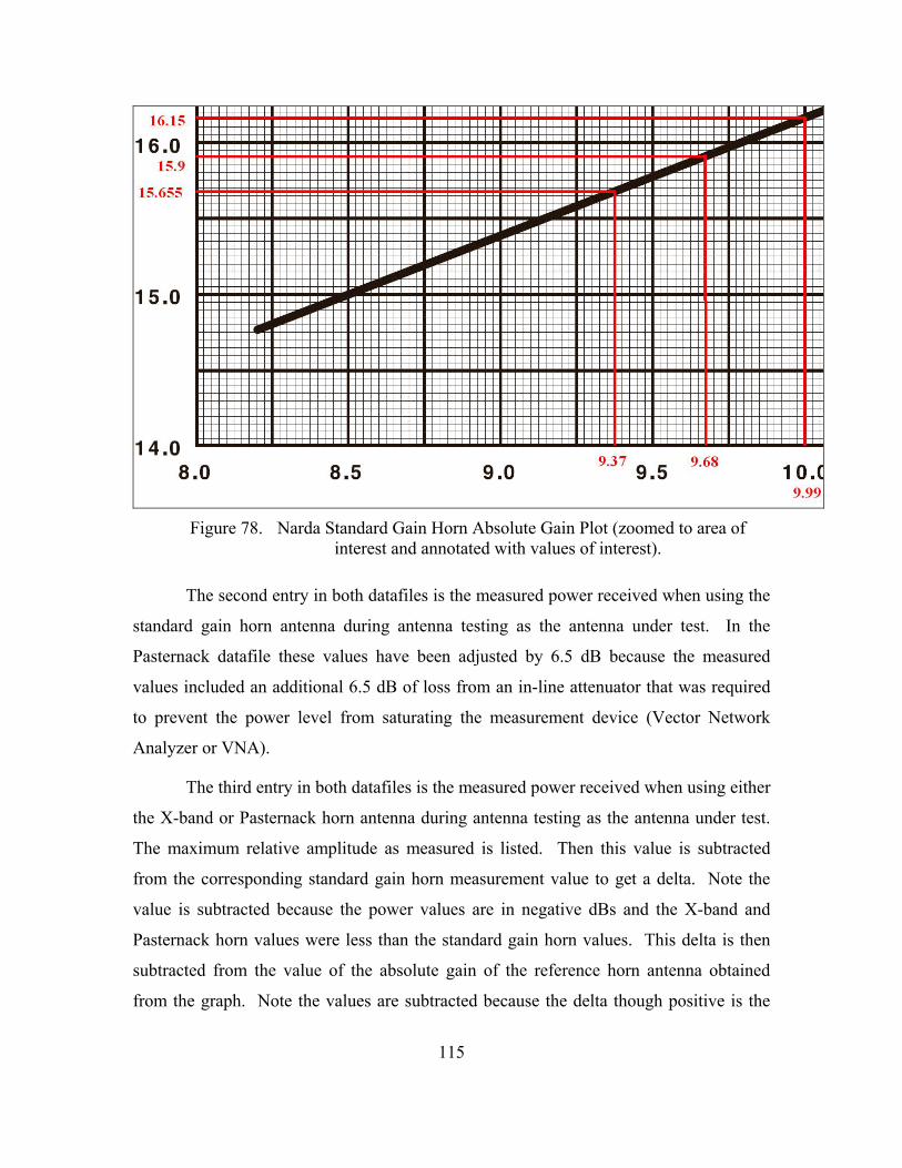
115
Figure 78. Narda Standard Gain Horn Absolute Gain Plot (zoomed to area of
interest and annotated with values of interest).
The second entry in both datafiles is the measured power received when using the
standard gain horn antenna during antenna testing as the antenna under test. In the
Pasternack datafile these values have been adjusted by 6.5 dB because the measured
values included an additional 6.5 dB of loss from an in-line attenuator that was required
to prevent the power level from saturating the measurement device (Vector Network
Analyzer or VNA).
The third entry in both datafiles is the measured power received when using either
the X-band or Pasternack horn antenna during antenna testing as the antenna under test.
The maximum relative amplitude as measured is listed. Then this value is subtracted
from the corresponding standard gain horn measurement value to get a delta. Note the
value is subtracted because the power values are in negative dBs and the X-band and
Pasternack horn values were less than the standard gain horn values. This delta is then
subtracted from the value of the absolute gain of the reference horn antenna obtained
from the graph. Note the values are subtracted because the delta though positive is the
116
amount below in power. The result is the absolute gain for that antenna at the given
frequency.
Then the value for the first measurement to exceed 3 dB below the maximum
relative amplitude is listed along with its angle in degrees. This was done for both the
first value above and below in angle of the maximum relative amplitude angle. These
angle values were subtracted from one another to find the 3dB Beamwidth.
Example calculation from X-band Horn #1 at 9.37 GHz in the E plane (as
described above):
Absolute Gain:
( 12.43115) ( 15.18115) 2.75 dB15.655 2.75 12.905 dB− − − =
− =
3dB Beamwidth:
17 ( 15) 32 dB− − =
F. ANTENNA ISOLATION TEST DATA
At 80 cm separation from each other oriented main beam parallel to each other
both at horizontal polarization the isolation between the antennas was found to be -42 dB.
At cross polarization (one horizontal and one vertical) the isolation was found to be -57
dB. At slant 45° degree polarization (parallel, then perpendicular) the isolation was
found to be -47 dB. At twice the separation distance (160 cm), the isolation increased by
6 dB (to -48 dB from -42 dB for co-polarization horizontal). This demonstrated the drop-
off from spreading loss alone (where twice the distance reduces power by a quarter). A
distance of 6 ft (same as lumber length) was chosen for the antenna separation and
mounting on the ACS. This was sufficient isolation to prevent regenerative feedback. In
addition to this minimum antenna separation distance an RF isolator was used to make
the ACS transmission path regenerative. There is a need for an RF isolator because all of
the RF components are bidirectional. When the RF amplifier was used (as in the
anechoic chamber testing) the isolator was not required, as an amplifier is a uni-
directional device. If the signal path through the ACS is allowed to be bi-directional,

117
then the horns become radiators in a two element array with large electrical spacing. This
results in a radiation pattern with numerous narrow lobes. This condition must be
eliminated if the ACS radiation pattern is to be that of a single horn.

118
THIS PAGE INTENTIONALLY LEFT BLANK

119
APPENDIX G. ANECHOIC CHAMBER
This appendix provides information on the setup of the Naval Postgraduate
School’s anechoic chamber on the roof of Spanagel Hall. This is the anechoic chamber
owned by the Electrical and Computer Engineering Department. This was the only
anechoic chamber used in this thesis (to include Antenna Testing and
Amplitude/Reflectivity Measurements).
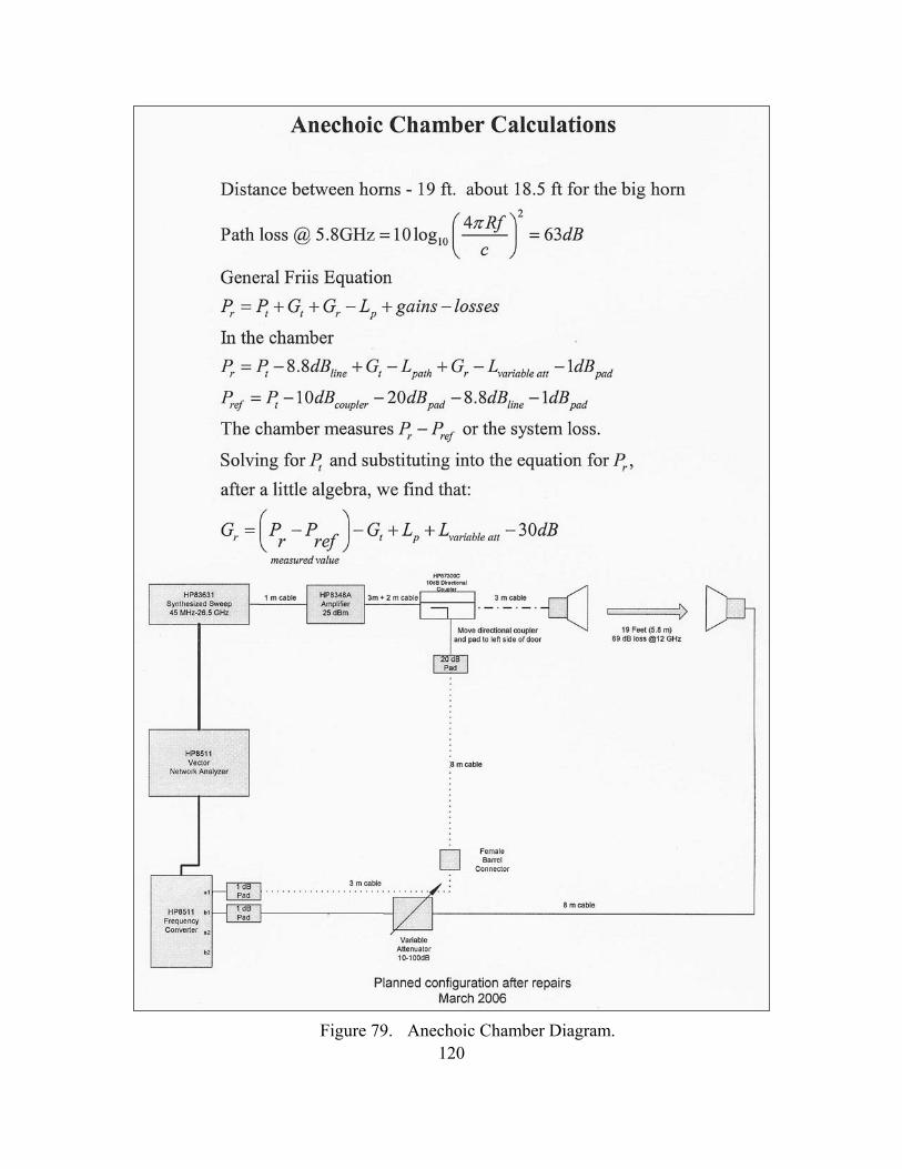
120
Figure 79. Anechoic Chamber Diagram.
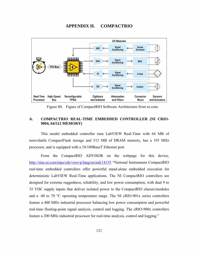
121
APPENDIX H. COMPACTRIO
Figure 80. Figure of CompactRIO Software Architecture from ni.com.
A. COMPACTRIO REAL-TIME EMBEDDED CONTROLLER (NI CRIO-9004, 64/512 MEMORY)
This model embedded controller runs LabVIEW Real-Time with 64 MB of
nonvolatile CompactFlash storage and 512 MB of DRAM memory, has a 195 MHz
processor, and is equipped with a 10/100BaseT Ethernet port.
From the CompactRIO ADVISOR on the webpage for this device,
http://sine.ni.com/nips/cds/view/p/lang/en/nid/14155 “National Instruments CompactRIO
real-time embedded controllers offer powerful stand-alone embedded execution for
deterministic LabVIEW Real-Time applications. The NI CompactRIO controllers are
designed for extreme ruggedness, reliability, and low power consumption, with dual 9 to
35 VDC supply inputs that deliver isolated power to the CompactRIO chassis/modules
and a -40 to 70 °C operating temperature range. The NI cRIO-901x series controllers
feature a 400 MHz industrial processor balancing low power consumption and powerful
real-time floating-point signal analysis, control and logging. The cRIO-900x controllers
feature a 200 MHz industrial processor for real-time analysis, control and logging.”
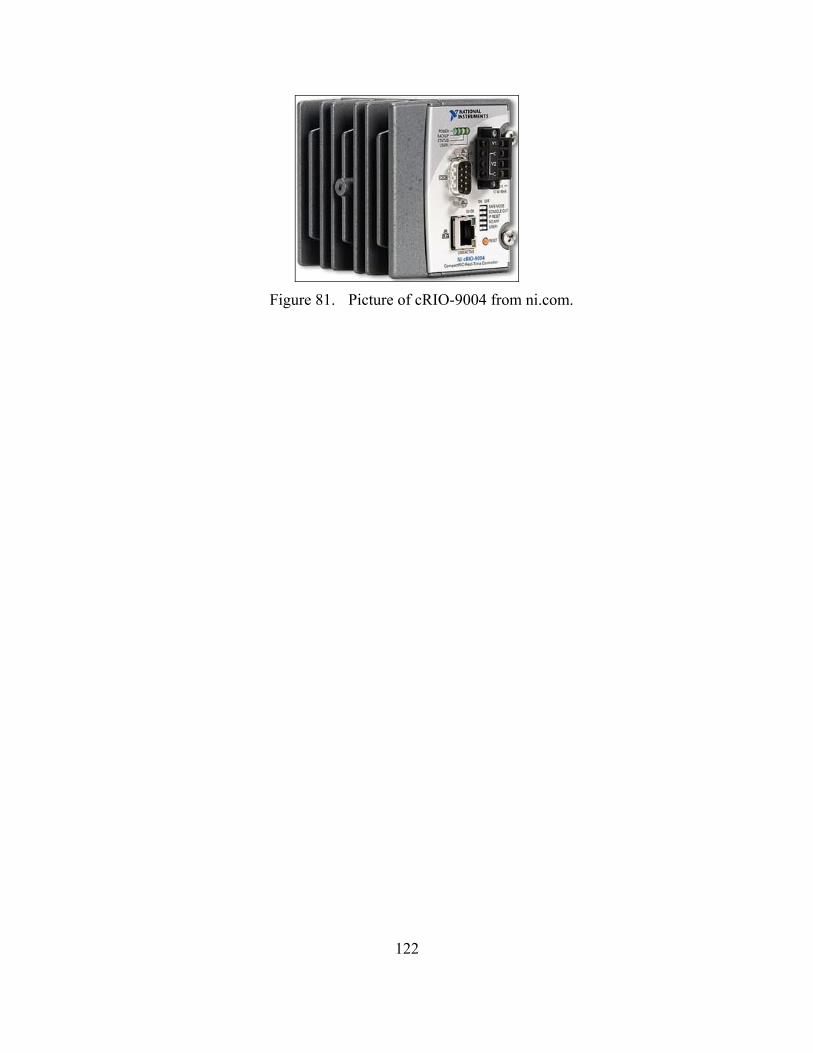
122
Figure 81. Picture of cRIO-9004 from ni.com.
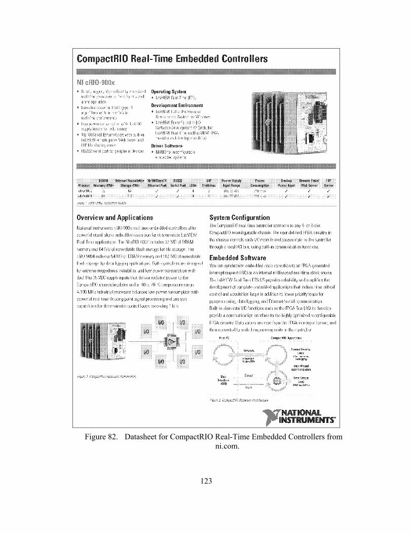
123
Figure 82. Datasheet for CompactRIO Real-Time Embedded Controllers from
ni.com.
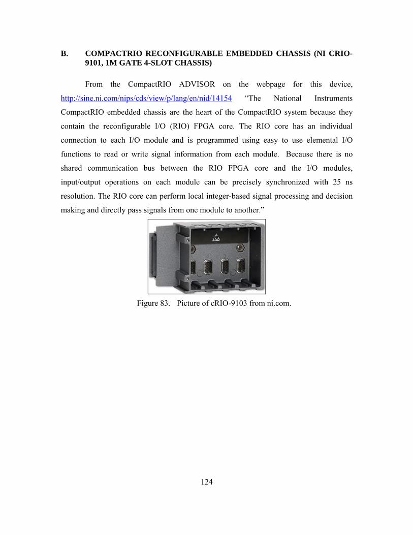
124
B. COMPACTRIO RECONFIGURABLE EMBEDDED CHASSIS (NI CRIO-9101, 1M GATE 4-SLOT CHASSIS)
From the CompactRIO ADVISOR on the webpage for this device,
http://sine.ni.com/nips/cds/view/p/lang/en/nid/14154 “The National Instruments
CompactRIO embedded chassis are the heart of the CompactRIO system because they
contain the reconfigurable I/O (RIO) FPGA core. The RIO core has an individual
connection to each I/O module and is programmed using easy to use elemental I/O
functions to read or write signal information from each module. Because there is no
shared communication bus between the RIO FPGA core and the I/O modules,
input/output operations on each module can be precisely synchronized with 25 ns
resolution. The RIO core can perform local integer-based signal processing and decision
making and directly pass signals from one module to another.”
Figure 83. Picture of cRIO-9103 from ni.com.
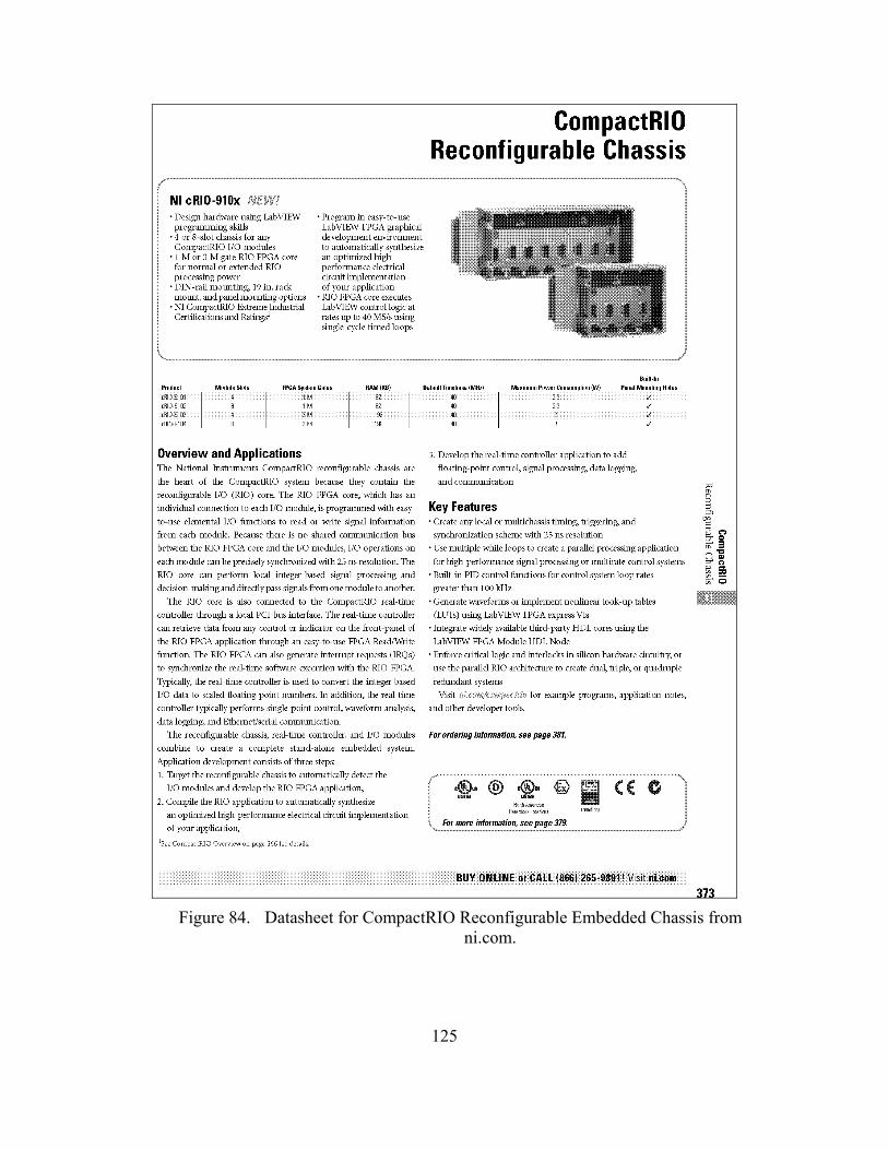
125
Figure 84. Datasheet for CompactRIO Reconfigurable Embedded Chassis from
ni.com.
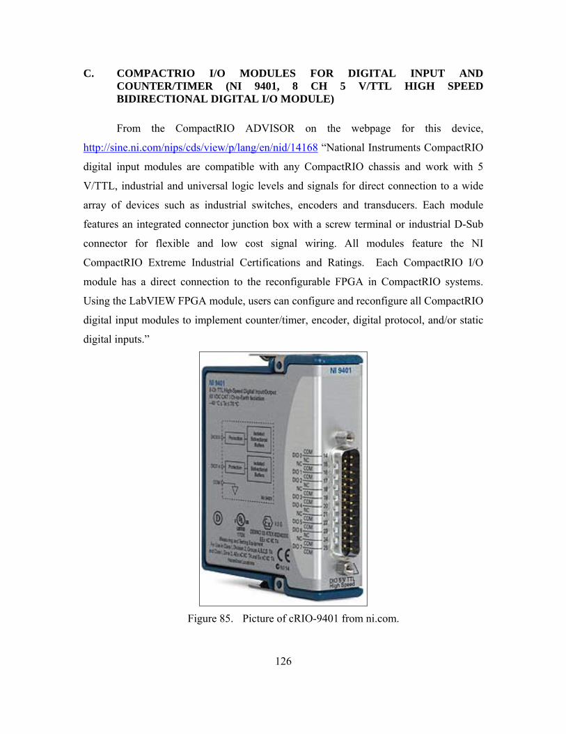
126
C. COMPACTRIO I/O MODULES FOR DIGITAL INPUT AND COUNTER/TIMER (NI 9401, 8 CH 5 V/TTL HIGH SPEED BIDIRECTIONAL DIGITAL I/O MODULE)
From the CompactRIO ADVISOR on the webpage for this device,
http://sine.ni.com/nips/cds/view/p/lang/en/nid/14168 “National Instruments CompactRIO
digital input modules are compatible with any CompactRIO chassis and work with 5
V/TTL, industrial and universal logic levels and signals for direct connection to a wide
array of devices such as industrial switches, encoders and transducers. Each module
features an integrated connector junction box with a screw terminal or industrial D-Sub
connector for flexible and low cost signal wiring. All modules feature the NI
CompactRIO Extreme Industrial Certifications and Ratings. Each CompactRIO I/O
module has a direct connection to the reconfigurable FPGA in CompactRIO systems.
Using the LabVIEW FPGA module, users can configure and reconfigure all CompactRIO
digital input modules to implement counter/timer, encoder, digital protocol, and/or static
digital inputs.”
Figure 85. Picture of cRIO-9401 from ni.com.
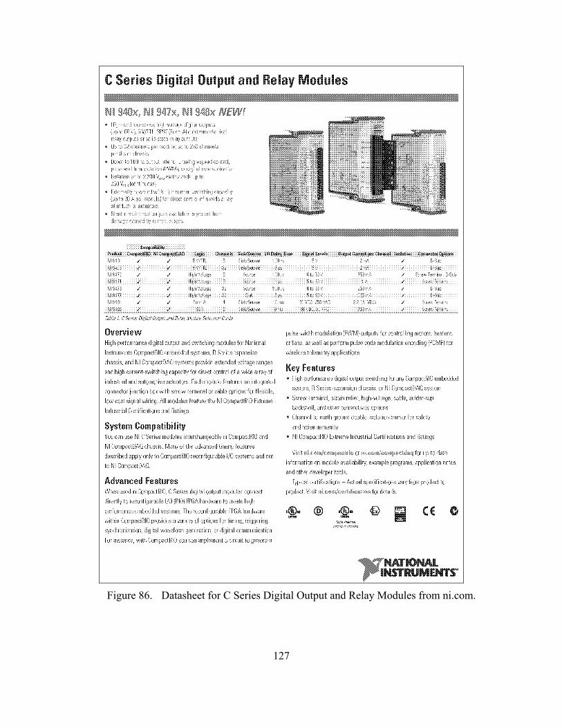
127
Figure 86. Datasheet for C Series Digital Output and Relay Modules from ni.com.

128
D. NI DEVELOPER SUITE WITH REAL-TIME AND FPGA SOFTWARE FOR COMPACTRIO
From the CompactRIO ADVISOR on the webpage for this software package,
http://sine.ni.com/nips/cds/view/p/lang/en/nid/14294 “The NI Developer Suite Core
Package with the Real-Time Deployment and FPGA Deployment options include all of
the tools you need for building a custom embedded system - LabVIEW FPGA for
customizing hardware I/O in the user-configurable FPGA core and LabVIEW Real-Time
for building deterministic and reliable real-time applications. The NI Developer Suite
Core Package with the Real-Time Deployment and FPGA Deployment options also
include a comprehensive set of LabVIEW add-on tools for algorithm development, real-
time development analysis, Microsoft Office report generation, and database
communication.”
Of particular note in this software package is the FPGA Deployment Option,
which includes the LabVIEW FPGA Module and NI RIO. These are essential
programming components to the LabVIEW software library used with the ACS. NI RIO
is needed to communicate with the CompactRIO Chassis(FPGAs) and the LabVIEW
FPGA module for programming commands that can be auto-compiled into VHDL for the
CompactRIO Chassis(FPGAs).
129
APPENDIX I. LABVIEW FOR THE DIGITAL PHASE SHIFTER
How the digital phase shifter is controlled by code written in LabVIEW and run on the
CRIO is explained here.
The LabVIEW Virtual Instruments (VIs) described here include: ManualControl,
PhaseShifterControl, MasterControl, and SlaveControl. Together they provide three
distinction functionalities in the development of the ACS’s software. These are the main
VIs. All VIs, including Block Diagram and Front Panel files for each, are included after
the description of these main VIs. The VIs not described are test components only and
not used with the ACS’s current functionalities, although they did play a part in its past
development and possibly future development and are included here for that purpose.
Primarily they were used to test certain functions that were later incorporated into the
main VIs or demonstrate alternative ways of implementing the same functionality as was
incorporated into the main VIs as part of testing method efficiency. These VIs include:
dataIO, fpgaRX_test, fpgaTX_test, NetworkRX_test, NetworkTX_test, and tDcalc.
KNORR-CAL_project is an overall view of the LabVIEW project with all VIs and
hardware indicated. The VI PSC6-bit is merely an example of how to modify the files
for a different number of control bits. When the ACS was first developed a 6-bit digital
phase shifter rather than an 8-bit digital phase shifter was used. The basic principle of
this modification is to globally find and replace the number representing 2^(current
number of bits) with 2^(future number of bits). For example, replace 255 (for 8-bit) with
63 (for 6-bit).
Observe the Block Diagram for each VI and follow along in the diagram left to right as
the description explains the graphical code.
A. PHASESHIFTERCONTROL
First, the count is reset (initialized) to zero. Then, the time delay (tD) is read in to
become the time between phase state changes. This is also referred to as ‘ticks’. 1 tick =
1 bit change = 25 ns (the time of one 40MHz clock cycle). The count is checked so as to
130
not exceed the number of phase shifter bits (phase states). Here there are 8-bits or
2^8=256 phase states. Since 0 is considered the first phase state, the count will increment
through all 256 phase states and stop at 255.
If the Doppler shift is going to be an up Doppler shift (increase in frequency) the
count proceeds unaltered, counting up. If the Doppler shift is to be a down Doppler shift
(decrease in frequency) the count proceeds inverted, counting down. The integer value of
the count is then converted into a Boolean value. For example, the integer value of 157 =
10011101. The Boolean value is then broken into each of its individual bits and routed to
the corresponding Digital I/O (DIO) pin to apply or remove voltage from the appropriate
phase shifter control pin. In this VI’s current state, both DIO modules receive the same
signal.
See Chapter on Future Work. Once the programmable attenuator is received, the
second group of DIO pins will be assigned to control this device with dependent
statistics. For independent statistics, a second PhaseShifterControl VI will need to be
created(duplicated and renamed AttenuatorControl). The only difference between the
original and its duplicate is that the duplicate DIOs will be deleted one from each VI so
that each VI contains only one unique set of DIO assignments. For dependent
(correlated) statistics the DIOs will be controlled from within the same VI in a
synchronized time delay (tD).
Once the commands for the appropriate voltages have been sent, the count
increments, and the process begins all over again. This process continues until one
complete cycle through all the phase states is completed (one period of 2π). Then, the
loop encounters an exit condition and the count is reset and the whole sequence begins
again (the next period of 2π).
B. SLAVECONTROL
Paired with MasterControl provides automatic PhaseShifterControl to work with
data read in from a file. The difference is that an array of integer values corresponding to
the tD is first read and stored. Then, the individual time delay integer values are used to
provide the appropriate phase shifter Doppler shift values as opposed to the manual entry
131
input by a user in the GUI of PhaseShifterControl. In addition, instead of a switch being
flipped by a user in the GUI to decide up or down Doppler shift, the sign of the integer
value is used. A negative sign is used to indicate a down shift and the absence of a
negative sign (i.e. positive) to indicate an up shift. Zero indicates no Doppler shift. The
process is then exactly the same as that implemented/programmed in PhaseShifterControl
(See section above by the same name).
*NOTE: the number of Doppler frequencies cannot be automatically detected from the
data file stored on the PC. The number of frequencies must be defined from within the
VI. This allows the appropriate sized array to be created in the software even before it
starts running. This is noted in the VI Front Panel (GUI) as well.
C. MASTERCONTROL
This VI reads in the value of the Doppler frequencies from a tab delaminated file
(such as how the array of variables would be exported/saved from the Weather Signal
Simulator in MATLAB). The numbers(frequencies) are read in as double floating point.
numtDs is the number of Doppler frequencies read in. The Doppler frequencies (DF) are
then used to calculate the Radial Velocity (Vr), Period (T), and Bit Delay (t) according to
the following relations:
Equation 1 2
cVr DFRF
= ××
in meters per second
Equation 2 1 1000TDF
= × in milliseconds
Equation 3 610
25Ttn
= in ‘ticks’ (of 25ns)
Where the RF Frequency (RF) is defined to be 9990000000Hz or 9.99GHz, the Speed of
Light (c) is 299792458 m/s, and the number of Phase Steps (n) is 63 (for 6 bits).
However, since only integers (INT) can be passed to the FPGA, the doubles
(DBL) are converted to integers and sent to the FPGA. The Period, DF, and Vr are then
recalculated based on these 16-bit integer values. This is to show the user what actual
values will be produced by the ACS. This only affects values stored in the data file
which may have been truncated by the conversion. This is a potential software limitation.
132
However, this will not affect the calibration process, only “real world” weather
simulation, because any variation from the input values that have been truncated are now
recomputed and displayed to the user. The radar should be tested/calibrated to agree with
these values, not the values output by the Weather Signal Simulator. This is a limitation
of the calibrator’s software when interacting with the FPGA. Although values may be
calculated accurately by the Weather Signal Simulator to agree with “real world” weather
patterns, the calibrator cannot always reproduce these exact values. This is a hardware
limitation due to the FPGA and seen in the software. In practice, this limitation is similar
to other hardware limitations already discussed. See Hardware Limitations Section.
*NOTE: before executing the VI, the array size in SlaveControl must be defined to the
number of Doppler frequencies intended to be read from the data file. This is not
automatic. It cannot predetermine the number of entries. There is no “read until end of
file.” See also SlaveControl NOTE.
*NOTE: the path on the PC to the data file must be entered into the VI. The data file
must be a single row of tab delaminated Doppler frequency entries stored in a text file
(.txt) where a negative sign indicates a down Doppler shift and no sign indicates an up
Doppler shift. Do not use + signs.
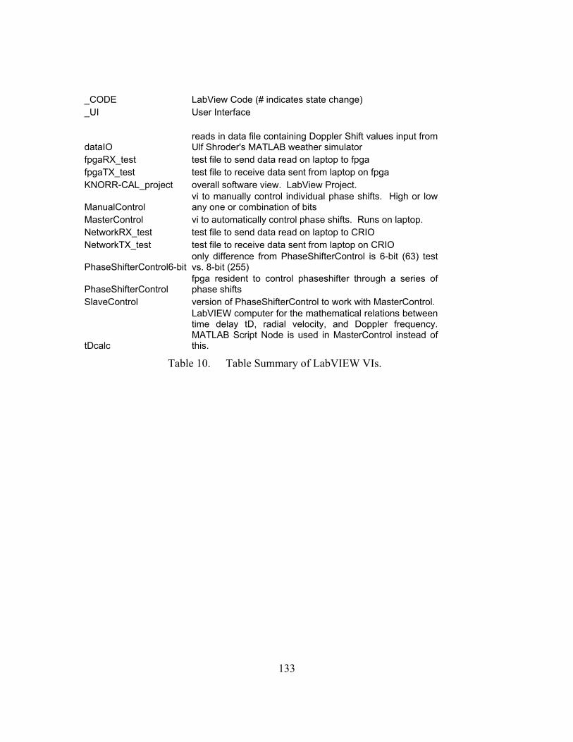
133
_CODE LabView Code (# indicates state change) _UI User Interface
dataIO reads in data file containing Doppler Shift values input from Ulf Shroder's MATLAB weather simulator
fpgaRX_test test file to send data read on laptop to fpga fpgaTX_test test file to receive data sent from laptop on fpga KNORR-CAL_project overall software view. LabView Project.
ManualControl vi to manually control individual phase shifts. High or low any one or combination of bits
MasterControl vi to automatically control phase shifts. Runs on laptop. NetworkRX_test test file to send data read on laptop to CRIO NetworkTX_test test file to receive data sent from laptop on CRIO
PhaseShifterControl6-bit only difference from PhaseShifterControl is 6-bit (63) test vs. 8-bit (255)
PhaseShifterControl fpga resident to control phaseshifter through a series of phase shifts
SlaveControl version of PhaseShifterControl to work with MasterControl.
tDcalc
LabVIEW computer for the mathematical relations between time delay tD, radial velocity, and Doppler frequency. MATLAB Script Node is used in MasterControl instead of this.
Table 10. Table Summary of LabVIEW VIs.
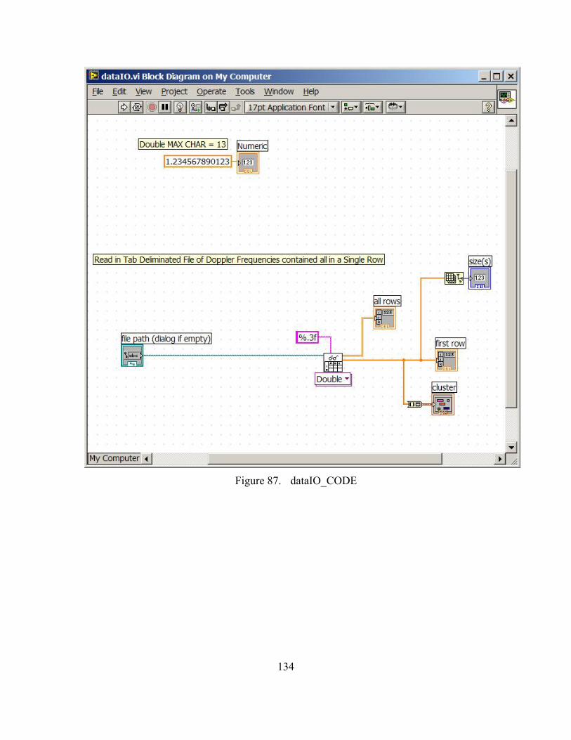
134
Figure 87. dataIO_CODE
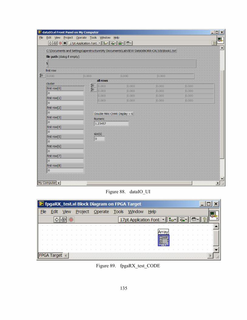
135
Figure 88. dataIO_UI
Figure 89. fpgaRX_test_CODE
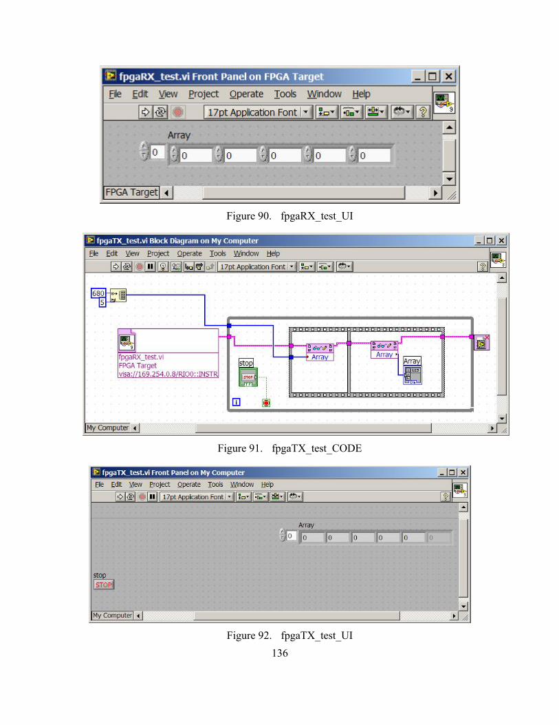
136
Figure 90. fpgaRX_test_UI
Figure 91. fpgaTX_test_CODE
Figure 92. fpgaTX_test_UI
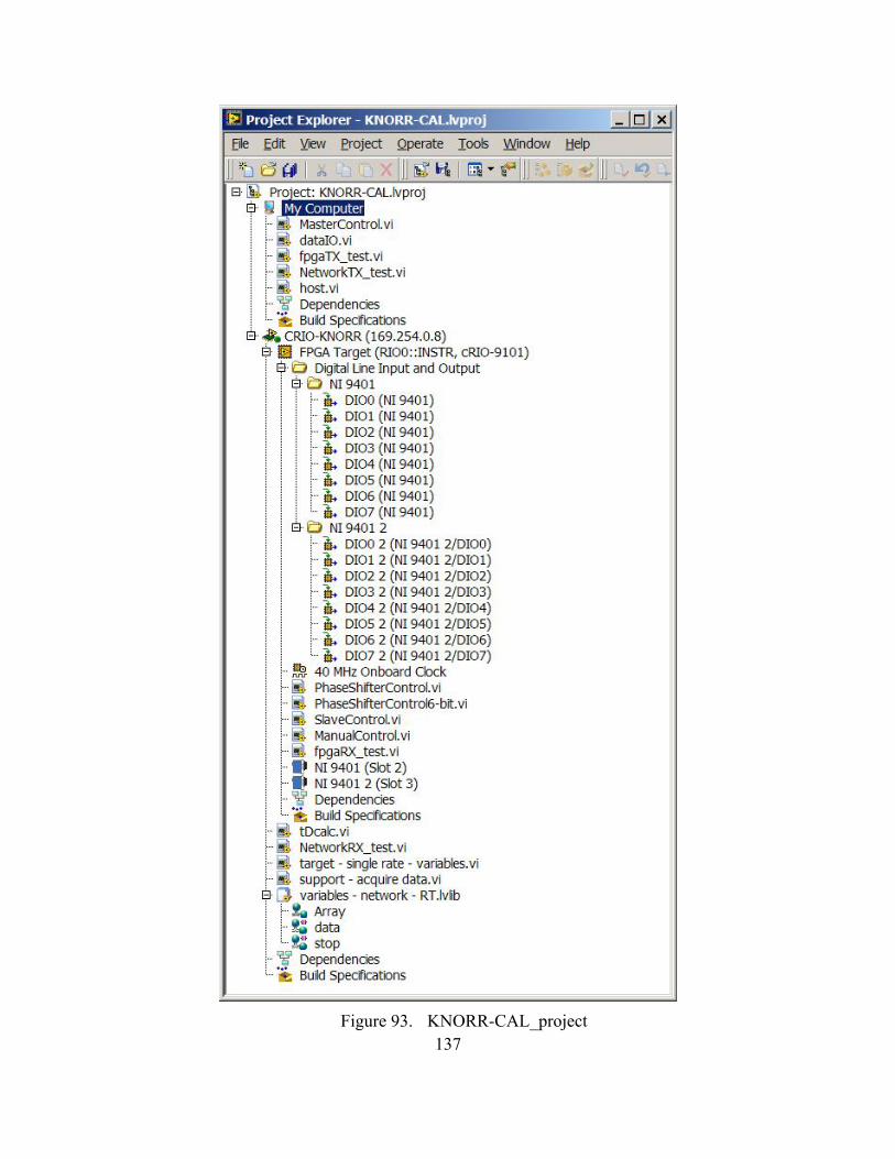
137
Figure 93. KNORR-CAL_project
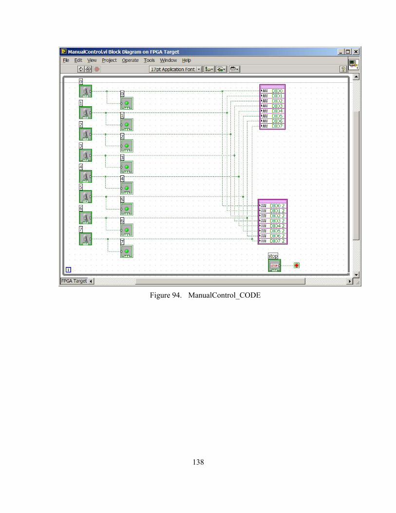
138
Figure 94. ManualControl_CODE
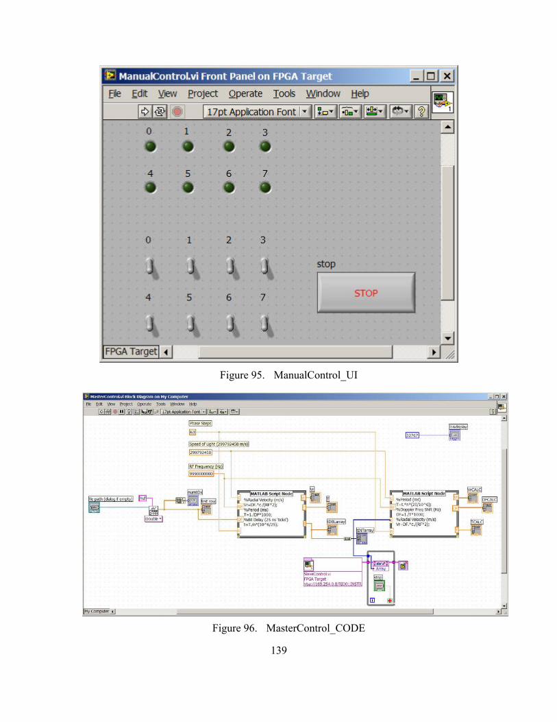
139
Figure 95. ManualControl_UI
Figure 96. MasterControl_CODE
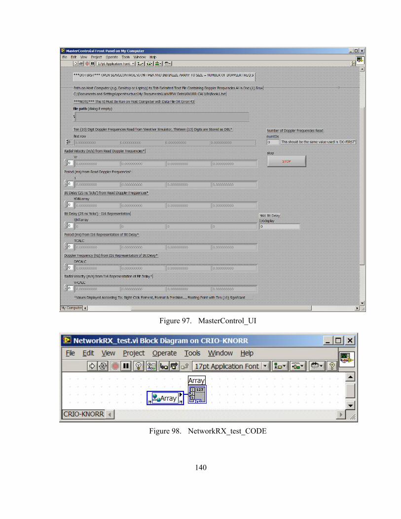
140
Figure 97. MasterControl_UI
Figure 98. NetworkRX_test_CODE
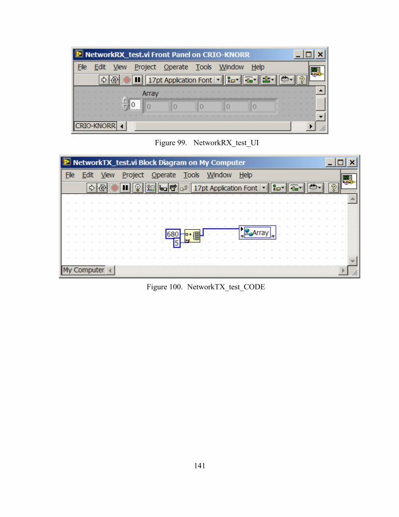
141
Figure 99. NetworkRX_test_UI
Figure 100. NetworkTX_test_CODE

142
Figure 101. PhaseShifterControl6-bit_CODE1
Figure 102. PhaseShifterControl6-bit_CODE2
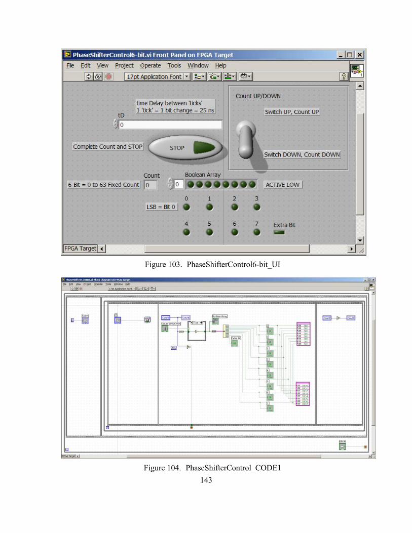
143
Figure 103. PhaseShifterControl6-bit_UI
Figure 104. PhaseShifterControl_CODE1
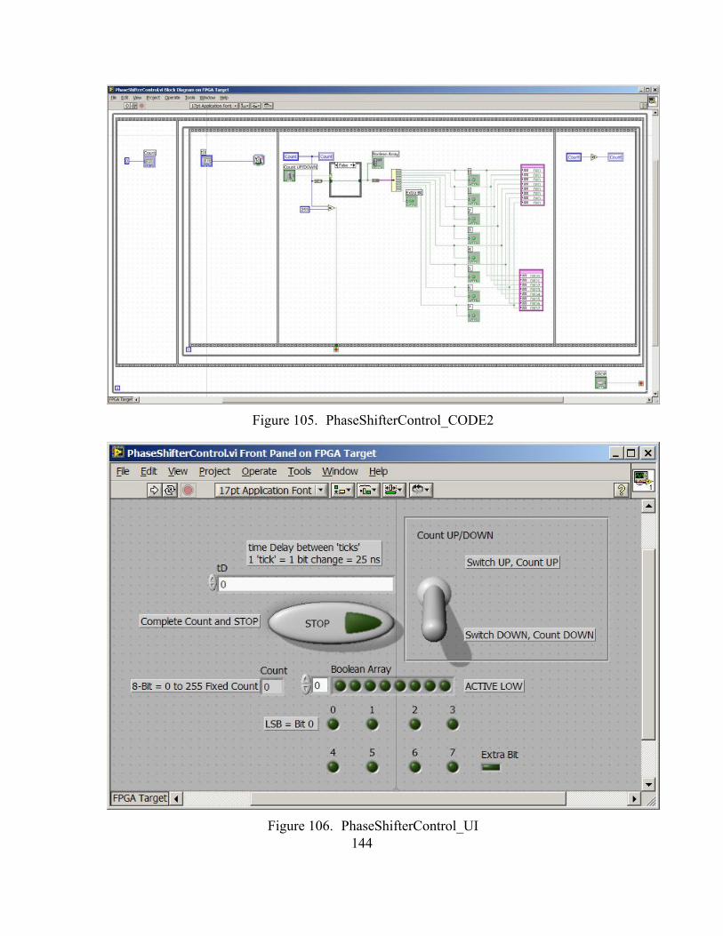
144
Figure 105. PhaseShifterControl_CODE2
Figure 106. PhaseShifterControl_UI
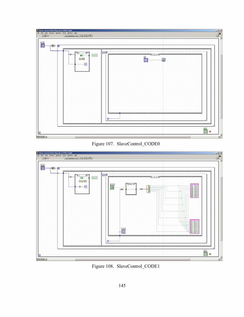
145
Figure 107. SlaveControl_CODE0
Figure 108. SlaveControl_CODE1
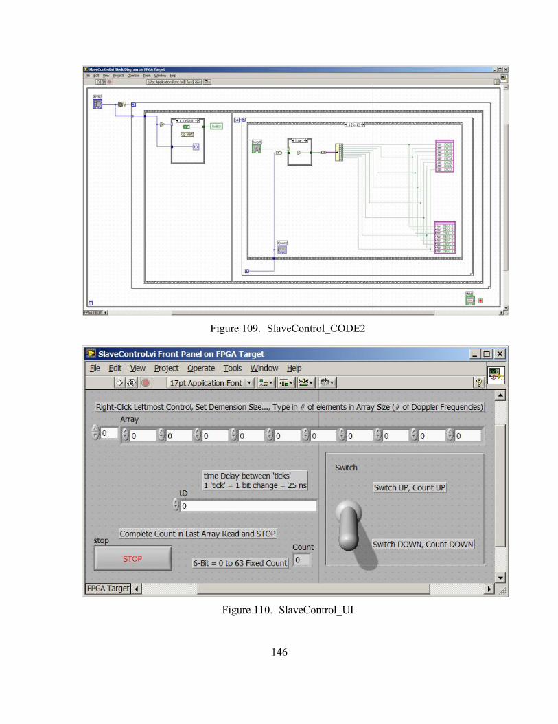
146
Figure 109. SlaveControl_CODE2
Figure 110. SlaveControl_UI
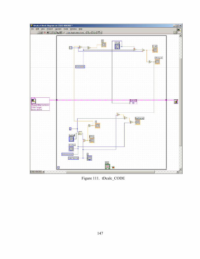
147
Figure 111. tDcalc_CODE
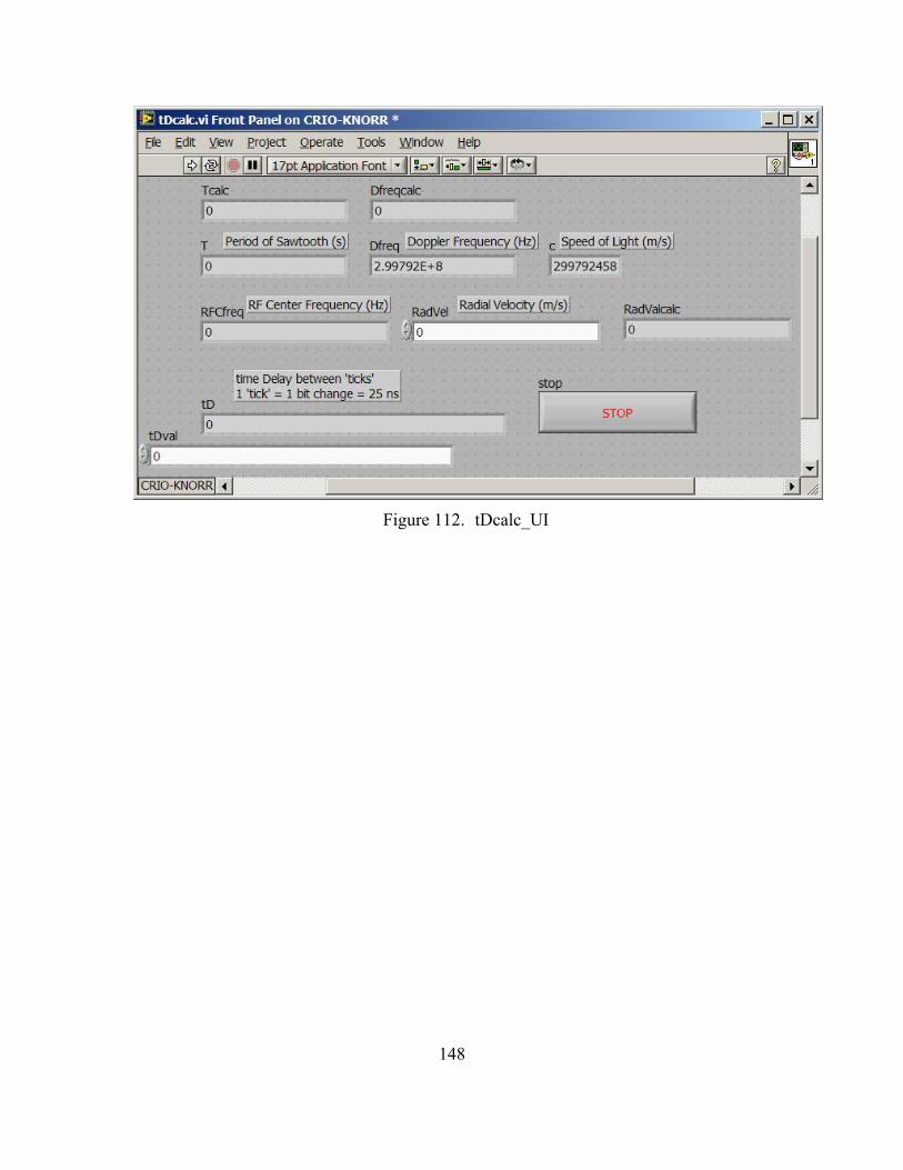
148
Figure 112. tDcalc_UI
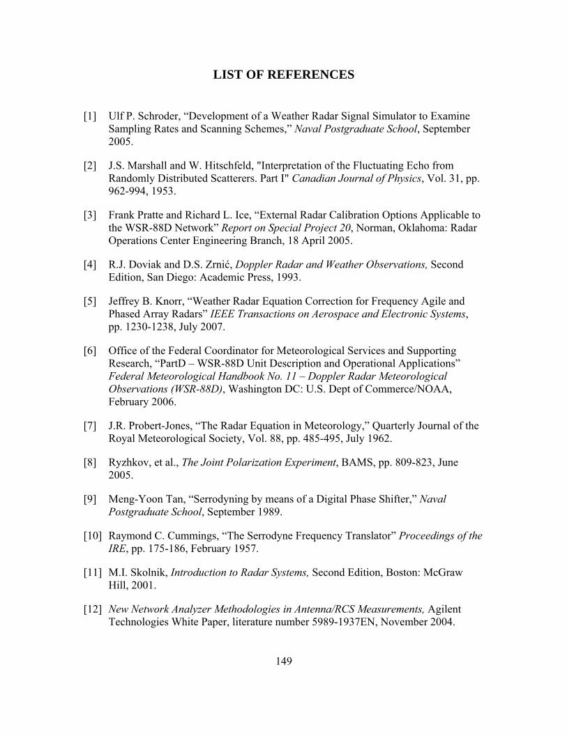
149
LIST OF REFERENCES
[1] Ulf P. Schroder, “Development of a Weather Radar Signal Simulator to Examine Sampling Rates and Scanning Schemes,” Naval Postgraduate School, September 2005.
[2] J.S. Marshall and W. Hitschfeld, "Interpretation of the Fluctuating Echo from Randomly Distributed Scatterers. Part I" Canadian Journal of Physics, Vol. 31, pp. 962-994, 1953.
[3] Frank Pratte and Richard L. Ice, “External Radar Calibration Options Applicable to the WSR-88D Network” Report on Special Project 20, Norman, Oklahoma: Radar Operations Center Engineering Branch, 18 April 2005.
[4] R.J. Doviak and D.S. Zrnić, Doppler Radar and Weather Observations, Second Edition, San Diego: Academic Press, 1993.
[5] Jeffrey B. Knorr, “Weather Radar Equation Correction for Frequency Agile and Phased Array Radars” IEEE Transactions on Aerospace and Electronic Systems, pp. 1230-1238, July 2007.
[6] Office of the Federal Coordinator for Meteorological Services and Supporting Research, “PartD – WSR-88D Unit Description and Operational Applications” Federal Meteorological Handbook No. 11 – Doppler Radar Meteorological Observations (WSR-88D), Washington DC: U.S. Dept of Commerce/NOAA, February 2006.
[7] J.R. Probert-Jones, “The Radar Equation in Meteorology,” Quarterly Journal of the Royal Meteorological Society, Vol. 88, pp. 485-495, July 1962.
[8] Ryzhkov, et al., The Joint Polarization Experiment, BAMS, pp. 809-823, June 2005.
[9] Meng-Yoon Tan, “Serrodyning by means of a Digital Phase Shifter,” Naval Postgraduate School, September 1989.
[10] Raymond C. Cummings, “The Serrodyne Frequency Translator” Proceedings of the IRE, pp. 175-186, February 1957.
[11] M.I. Skolnik, Introduction to Radar Systems, Second Edition, Boston: McGraw Hill, 2001.
[12] New Network Analyzer Methodologies in Antenna/RCS Measurements, Agilent Technologies White Paper, literature number 5989-1937EN, November 2004.

150
THIS PAGE INTENTIONALLY LEFT BLANK

151
INITIAL DISTRIBUTION LIST
1. Defense Technical Information Center Ft. Belvoir, Virginia
2. Dudley Knox Library Naval Postgraduate School Monterey, California
3. Professor Jeffrey B. Knorr Chairman, Code EC Department of Electrical and Computer Engineering Naval Postgraduate School Monterey, California
4. Professor Dan C. Boger Chairman, Code IW Department of Information Sciences Naval Postgraduate School Monterey, California
5. Terry E. Smith, Lt Col, USAF Department of Information Sciences Naval Postgraduate School Monterey, California
6. Robert Broadston Department of Electrical and Computer Engineering Naval Postgraduate School Monterey, California
7. Paul Buczynski Department of Electrical and Computer Engineering Naval Postgraduate School Monterey, California
8. Professor David C. Jenn Department of Electrical and Computer Engineering Naval Postgraduate School Monterey, California