Embed Size (px)
Citation preview
University of Calgary
PRISM: University of Calgary's Digital Repository
Graduate Studies The Vault: Electronic Theses and Dissertations
2017
Design and Implementation of Single Transistor
Active Filters
Poddar, Neethila Nabanita
Poddar, N. N. (2017). Design and Implementation of Single Transistor Active Filters (Unpublished
master's thesis). University of Calgary, Calgary, AB. doi:10.11575/PRISM/25573
http://hdl.handle.net/11023/3538
master thesis
University of Calgary graduate students retain copyright ownership and moral rights for their
thesis. You may use this material in any way that is permitted by the Copyright Act or through
licensing that has been assigned to the document. For uses that are not allowable under
copyright legislation or licensing, you are required to seek permission.
Downloaded from PRISM: https://prism.ucalgary.ca

UNIVERSITY OF CALGARY
Design and Implementation of Single Transistor Active Filters
by
Neethila Nabanita Poddar
A THESIS
SUBMITTED TO THE FACULTY OF GRADUATE STUDIES
IN PARTIAL FULFILMENT OF THE REQUIREMENTS FOR THE
DEGREE OF MASTER OF SCIENCE
GRADUATE PROGRAM IN ELECTRICAL ENGINEERING
CALGARY, ALBERTA
January, 2017
© Neethila Nabanita Poddar 2017
Abstract
This thesis investigates the design of single transistor second order active filters. Four gen-
eral topologies are presented, each with a two port network surrounded by three impedances
that form a T-network. From the topologies, four transfer functions are derived which are
further simplified by replacing the two port transmission matrix parameters with those of
an ideal MOS. An exhaustive MAPLE search code is used to generate all possible second
order filters. The search is carried out on the four general transfer functions, considering
all possible impedance combinations. Design procedures of selected filters are shown and
verified by Cadence Spectre simulations and experimental measurements. Based on the
single transistor second order filters, active realizations of higher order filters are explored.
A fourth order bandpass Chebyshev filter and a fourth order Comb filter are presented.
Simulation and experimental results of the designed filters are shown and compared with
the theoretical ones.
ii

Acknowledgements
I am thankful to the Almighty for giving me the opportunity to pursue graduate studies and
for helping me complete this work.
This thesis has been possible due to the continual support, advice and guidance of my
supervisor, Dr. Brent Maundy. I am very grateful for his helpful guidelines and constructive
feedbacks throughout the course of my graduate studies that enabled the completion of this
thesis. Also, I take this opportunity to gratefully acknowledge his understanding, patience
and continued supervision after my foot injury.
I would like to thank the ECE staffs Garwin and Chris for their help and suggestions
during the experimental implementation stage of my thesis. I am also grateful to my friends
and fellow graduate students for the useful discussions.
I express my heartfelt gratitude to my family for their love, support and motivation.
iii

Table of Contents
Abstract ii
Acknowledgements iii
Table of Contents iv
List of Tables vi
List of Figures vi
1 Introduction 11.1 Analog Filters . . . . . . . . . . . . . . . . . . . . . . . . . . . . . . . . . 11.2 Filter Classification . . . . . . . . . . . . . . . . . . . . . . . . . . . . . . 21.3 Allpass Filter . . . . . . . . . . . . . . . . . . . . . . . . . . . . . . . . . 41.4 Bandpass Filter . . . . . . . . . . . . . . . . . . . . . . . . . . . . . . . . 51.5 Bandstop or Notch Filter . . . . . . . . . . . . . . . . . . . . . . . . . . . 61.6 Higher Order Filter Design . . . . . . . . . . . . . . . . . . . . . . . . . . 71.7 Research Objectives . . . . . . . . . . . . . . . . . . . . . . . . . . . . . . 81.8 Thesis Overview . . . . . . . . . . . . . . . . . . . . . . . . . . . . . . . 9
2 Single Transistor Active Filter 112.1 Proposed General Three Impedance Filter Topologies . . . . . . . . . . . . 112.2 Variation of Type-3 Filter Structure . . . . . . . . . . . . . . . . . . . . . . 162.3 All possible filter types . . . . . . . . . . . . . . . . . . . . . . . . . . . . 172.4 Discussion of Selected Filters . . . . . . . . . . . . . . . . . . . . . . . . . 18
2.4.1 Bandpass Filter . . . . . . . . . . . . . . . . . . . . . . . . . . . . 192.4.1.1 Input and Output impedance of Bandpass Filter . . . . . 22
2.4.2 Bandstop or Notch Filter . . . . . . . . . . . . . . . . . . . . . . . 252.4.2.1 Input and Output Impedance of the Bandstop Filter . . . 25
2.4.3 Allpass Filter . . . . . . . . . . . . . . . . . . . . . . . . . . . . . 27
iv

2.4.3.1 Input and Output Impedance of the Allpass Filter . . . . 282.4.4 Effect of gm . . . . . . . . . . . . . . . . . . . . . . . . . . . . . . 292.4.5 Biasing Details . . . . . . . . . . . . . . . . . . . . . . . . . . . . 302.4.6 Non-ideal Effects . . . . . . . . . . . . . . . . . . . . . . . . . . . 32
2.4.6.1 Effect of ro . . . . . . . . . . . . . . . . . . . . . . . . . 322.4.6.2 Effect of parasitic capacitances . . . . . . . . . . . . . . 35
3 Simulation and Experimental Results 373.1 Bandpass Filter . . . . . . . . . . . . . . . . . . . . . . . . . . . . . . . . 373.2 Bandstop Filter . . . . . . . . . . . . . . . . . . . . . . . . . . . . . . . . 403.3 Allpass Filter . . . . . . . . . . . . . . . . . . . . . . . . . . . . . . . . . 42
4 A Fourth Order Chebyshev Filter 504.1 Classical Chebyshev Filter Design Approach . . . . . . . . . . . . . . . . 504.2 Proposed Fourth Order Chebyshev Filter . . . . . . . . . . . . . . . . . . 514.3 Simulated Results . . . . . . . . . . . . . . . . . . . . . . . . . . . . . . . 544.4 Two stage operational amplifier . . . . . . . . . . . . . . . . . . . . . . . . 54
4.4.1 Slew Rate . . . . . . . . . . . . . . . . . . . . . . . . . . . . . . . 574.4.2 Compensation of the two stage operational amplifier . . . . . . . . 58
4.5 Chebyshev filter cascaded with two stage operational amplifier . . . . . . . 594.6 Experimental Results . . . . . . . . . . . . . . . . . . . . . . . . . . . . . 60
5 A Novel Active Comb Filter 655.1 Proposed Comb Filter Structure . . . . . . . . . . . . . . . . . . . . . . . 655.2 Simulation Results . . . . . . . . . . . . . . . . . . . . . . . . . . . . . . 675.3 Experimental Results . . . . . . . . . . . . . . . . . . . . . . . . . . . . . 69
6 Conclusions and Future Work 756.1 Conclusion . . . . . . . . . . . . . . . . . . . . . . . . . . . . . . . . . . 756.2 Trade-offs . . . . . . . . . . . . . . . . . . . . . . . . . . . . . . . . . . . 766.3 Contribution . . . . . . . . . . . . . . . . . . . . . . . . . . . . . . . . . . 766.4 Future Work . . . . . . . . . . . . . . . . . . . . . . . . . . . . . . . . . . 77
Bibliography 79
v

List of Tables
2.1 Type-1, Type-2 and Type-3 transfer functions using an ideal transistor . . . 162.2 All possible second order filters for Type-1 filter configuration . . . . . . . 192.3 All possible second order filters for Type-2 filter structure . . . . . . . . . 202.4 All possible second order filters for Type-3 filter structure . . . . . . . . . 212.5 All possible filters of an altered Type-3 filter topology of Figure 2.4. . . . . 21
4.1 Chebyshev filter design equations for two stages . . . . . . . . . . . . . . 524.2 Deviation in experimental and PSPICE simulation results for Chebyshev
filter . . . . . . . . . . . . . . . . . . . . . . . . . . . . . . . . . . . . . . 61
5.1 Comb filter design equations for the two stages . . . . . . . . . . . . . . . 665.2 Deviation in experimental and PSPICE simulation results for Comb filter . 70
vi

List of Figures
1.1 Ideal brick wall magnitude response of (a) lowpass (b) highpass filters . . 31.2 Ideal brick wall magnitude response of (a) bandpass (b) bandstop filters . . 3
2.1 Type-1 filter topology with terminal A at AC ground . . . . . . . . . . . . 122.2 Type-2 filter structure with terminal C at AC ground . . . . . . . . . . . . 142.3 Type-3 filter topology with terminal B at AC ground . . . . . . . . . . . . 152.4 Altered Type-3 filter structure with Rs as an external resistor . . . . . . . . 162.5 Second order bandpass filter using a single transistor . . . . . . . . . . . . 222.6 General bandpass filter transfer function plotted in MATLAB at fo = 16.3
MHz, K = 0.99 and Q = 2.5 . . . . . . . . . . . . . . . . . . . . . . . . . 222.7 Small signal diagram to find Zout at very high and low frequencies . . . . . 242.8 Small signal diagram to find Zout at pole frequency . . . . . . . . . . . . . 242.9 Second order bandstop filter topology . . . . . . . . . . . . . . . . . . . . 252.10 General bandstop filter transfer function plotted in MATLAB for fo = 16.3
MHz, K = 0.99 and Q = 2 . . . . . . . . . . . . . . . . . . . . . . . . . . 262.11 Small signal diagram to find Zin of the notch circuit at very high frequencies 262.12 Second order AP filter structure . . . . . . . . . . . . . . . . . . . . . . . 282.13 General allpass filter transfer function plotted in MATLAB for fo = 16.3
MHz, K = 1 and Q = |Qz|= 1 . . . . . . . . . . . . . . . . . . . . . . . . 292.14 Allpass filter equivalent small signal diagram to find input impedance Zin
at very high frequencies . . . . . . . . . . . . . . . . . . . . . . . . . . . 302.15 Allpass filter equivalent small signal diagram to find output impedance Zout
at high frequencies . . . . . . . . . . . . . . . . . . . . . . . . . . . . . . 302.16 Allpass filter #1 from Table 2.5 implemented with an additional DC biasing
current source . . . . . . . . . . . . . . . . . . . . . . . . . . . . . . . . . 312.17 Simulated magnitude and phase responses of allpass filter of Figure 2.16 . 322.18 Simulated input and output waveforms of allpass filter of Figure 2.16 at
pole frequency of 4.6 MHz . . . . . . . . . . . . . . . . . . . . . . . . . . 33
vii

3.1 Magnitude response of proposed bandpass filter simulated in Cadence tovalues of L1= 50 µH, C1= 1.9 pF, R2=1.2 kΩ, R3=100 Ω, and Rs= 900 Ω. . 38
3.2 Cadence simulated transient responses of input and output signals of band-pass filter at pole frequency of 16.3 MHz to values L1= 50 µH, C1= 1.9 pF,R2= 1.2 kΩ, R3=100 Ω and Rs= 900 Ω. . . . . . . . . . . . . . . . . . . . 39
3.3 Measured magnitude response of bandpass filter to values of C1 = 680 pF,L1 = 10 mH, Rs = 900 Ω, R2 = 1.2 kΩ and R3 = 100 Ω. . . . . . . . . . . 40
3.4 Magnitude response of bandpass filter simulated in PSPICE to values ofC1 = 680 pF, L1 = 10 mH, Rs = 900 Ω, R2 = 1.2 kΩ and R3 = 100 Ω. . . . 41
3.5 Bandstop filter magnitude response simulated in Cadence to values of L1=10 µH, C1= 9.52 pF, R2= 600 Ω, R3=110 Ω, and Rs= 1.2 kΩ. . . . . . . . . 42
3.6 Cadence simulated input and output waveforms of bandstop filter at thepole frequency of 16.2 MHz to values L1= 10 µH, C1= 9.52 pF, R2= 600Ω, R3=110 Ω, and Rs= 1.2 kΩ. . . . . . . . . . . . . . . . . . . . . . . . . 43
3.7 Measured magnitude response of bandstop filter to values of C1 = 68 pF,L1 = 2 mH, Rs = 1.2 kΩ, R2 = 500 Ω and R3 = 100 Ω with a verticalscale of 5 dB/ division and a logarithmic horizontal scale where each cyclerepresents a factor of 10. . . . . . . . . . . . . . . . . . . . . . . . . . . . 44
3.8 Magnitude response of bandstop filter simulated in PSPICE to values ofC1 = 68 pF, L1 = 2 mH, Rs = 1.2 kΩ, R2 = 500 Ω and R3 = 100 Ω. . . . . 45
3.9 Allpass filter magnitude and phase response simulated in Cadence to valuesL2= 24 µH, C2= 50 pF, R1= 50 Ω, R3=930 Ω and Rs= 500 Ω. . . . . . . . 46
3.10 Cadence simulated input and output waveforms of allpass filter at pole fre-quency to values L2= 24 µH, C2= 50 pF, R1= 50 Ω, R3=930 Ω and Rs= 500Ω. . . . . . . . . . . . . . . . . . . . . . . . . . . . . . . . . . . . . . . . 47
3.11 Measured magnitude and phase response of allpass filter to values C1 = 68pF, L1 = 2 mH, R1 = 1 kΩ, R3 = 1.2 kΩ and Rs = 3.3 kΩ. . . . . . . . . . 48
3.12 Magnitude response of allpass filter simulated in PSPICE to values of C1 =
68 pF, L1 = 2 mH, R1 = 1 kΩ, R3 = 1.2 kΩ and Rs = 3.3 kΩ. . . . . . . . 49
4.1 Proposed Chebyshev fourth order bandpass filter . . . . . . . . . . . . . . 514.2 Passive fourth order bandpass filter . . . . . . . . . . . . . . . . . . . . . 524.3 Source follower used as a voltage buffer . . . . . . . . . . . . . . . . . . . 534.4 Comparison between ideal (dashed line) and simulated (solid line) magni-
tude and phase responses of Chebyshev filter . . . . . . . . . . . . . . . . 554.5 Two stage operational amplifier [33, 34] . . . . . . . . . . . . . . . . . . . 56
viii

4.6 Small signal diagram of a common source amplifier . . . . . . . . . . . . 574.7 Small signal model of two stage operational amplifier . . . . . . . . . . . 594.8 Magnitude and phase response of two stage operational amplifier simulated
in Cadence . . . . . . . . . . . . . . . . . . . . . . . . . . . . . . . . . . 604.9 Two stage opamp cascaded with fourth order Chebyshev filter of Figure 4.1
to improve overall gain of the filter . . . . . . . . . . . . . . . . . . . . . 614.10 Magnitude response of the proposed Chebyshev filter after cascading with
a two stage opamp . . . . . . . . . . . . . . . . . . . . . . . . . . . . . . 624.11 Measured magnitude response of the fourth order Chebyshev filter for com-
ponent values C1 = 6.8 nF, L1 = 1 mH, C2 = 2.2 nF, L2 = 2 mH, Rs = 900Ω, R2 = R4 = 1 kΩ and R3 = R5 = 100 Ω with a vertical scale of 3dB/division and horizontal scale of 20 kHz/ division. . . . . . . . . . . . . . . 63
4.12 Magnitude response of fourth order Chebyshev filter simulated in PSPICEfor component values C1 = 6.8 nF, L1 = 1 mH, C2 = 2.2 nF, L2 = 2 mH,Rs = 900 Ω, R2 = R4 = 1 kΩ and R3 = R5 = 100 Ω. . . . . . . . . . . . . 64
5.1 Proposed active fourth order comb filter . . . . . . . . . . . . . . . . . . . 665.2 Passive fourth order Comb filter . . . . . . . . . . . . . . . . . . . . . . . 665.3 Magnitude and phase responses of a general comb filter transfer function
given by equation (5.1) plotted in MATLAB for fo1 = 16.3 MHz, fo2 = 163MHz, Q = 3 and K1 = K2 = 0.99. . . . . . . . . . . . . . . . . . . . . . . 68
5.4 Cadence simulated magnitude response of fourth order comb filter for val-ues C1 = 9.5 pF, L1 = 10 µH, C2 = 0.95 pF, L2 = 1 µH, Rs = 1.2 kΩ,R2 = R4 = 600 Ω and R3 = R5 = 110 Ω. . . . . . . . . . . . . . . . . . . . 69
5.5 Input (V in) and output (Vo) waveforms of Comb filter in Figure 5.1 at fo1 =
16.2 MHz simulated in Cadence . . . . . . . . . . . . . . . . . . . . . . . 705.6 Input (V in) and output (Vo) waveforms of Comb filter in Figure 5.1 at fo2 =
162 MHz simulated in Cadence . . . . . . . . . . . . . . . . . . . . . . . 715.7 Cadence simulated response of comb filter designed to remove power line
interferences at 50 Hz and 150 Hz . . . . . . . . . . . . . . . . . . . . . . 725.8 Measured magnitude response of comb filter implemented using discrete
components of values C1 = 2.2 nF, L1 = 10 mH, C2 = 33 pF, L2 = 2 mH,Rs = 1.2 kΩ, R2 = R4 = 500 Ω and R3 = R5 = 100 Ω with a vertical scaleof 5dB/ division and a logarithmic horizontal scale where each cycle rep-resents a factor of 10. . . . . . . . . . . . . . . . . . . . . . . . . . . . . . 73
ix

5.9 Magnitude response of fourth order Comb filter simulated in PSPICE forcomponent values C1 = 2.2 nF, L1 = 10 mH, C2 = 33 pF, L2 = 2 mH,Rs = 1.2 kΩ, R2 = R4 = 500 Ω and R3 = R5 = 100 Ω. . . . . . . . . . . . 74
x

CHAPTER 1
Introduction
1.1 Analog Filters
Analog filters are circuits that process signals in a frequency dependent manner, that is,
they pass signals of a certain frequency range while blocking other frequencies. The range
of frequencies that is allowed to pass is known as the passband, while the range of fre-
quencies that is attenuated is the stopband. Filters can be passive or active. Passive filters
are based on combinations of resistors, capacitors and inductors. They do not require ex-
ternal power supply and do not use any active elements such as transistors or operational
amplifiers. Whereas, active filters are implemented by a combination of passive and active
components (transistors, op-amps) and operate off an external power supply. The basic
set of specifications that define a filter’s response are its passband frequency, stopband fre-
quency and gain characteristics at its passband and stopband. A filter’s gain is the ratio of
its output signal V 2 to its input signal V 1 and is usually expressed in decibels. Gain GdB is
defined as
GdB = 20log |T (ω)|dB (1.1)
where
|T (ω)|=∣∣∣∣V2 (ω)
V1 (ω)
∣∣∣∣ (1.2)
The term attenuation is also used instead of gain. It is simply the inverse of gain and can
be defined as
1

α (ω) = − 20log |T (ω)|dB, |T (ω)| ≤ 1 (1.3)
Real world signals have both wanted and unwanted components. Therefore, to view
signals at the desired frequency range it is essential to remove signals at other frequencies
by means of filtering. Filters are used widely in almost every electronic equipments, from
everyday electronics such as computers, radios, televisions, and stereo systems to equip-
ments such as spectrum analyzers and signal generators. Analog to digital converters also
require analog filters to prevent aliasing [1].
1.2 Filter Classification
The frequency selective characteristic of filter circuits can be used to differentiate between
the types of filters. A filter can have a lowpass, highpass, bandpass, bandstop and allpass
response where each name indicates the shape of the output waveform. For example, a
lowpass filter will pass signals of frequencies lower than a certain cutoff frequency while
attenuate the frequencies higher than the cutoff frequency. The ideal responses of lowpass
and highpass filters are shown in Figure 1.1. An ideal filter, also called a brick wall filter
transmits frequency in its passband completely unattenuated and without phase shift, while
providing full attenuation of signal components in the stopband. Figure 1.2 shows the ideal
responses of bandpass and bandstop filters. In practice, it is impossible to realise ideal or
brick wall filters. Realistic filter responses are referred to as approximations to the original.
There are different ways to approximate the characteristics of an ideal filter based on the
specifications. Some approximation methods used in analog filter design are Butterworth,
Chebyshev, Inverse Chebyshev, Elliptic or Cauer. In the following sections, some selected
filter types are discussed whose implementations are presented in Chapters 2 and 3.
2

Frequency
Gain
1StopbandPassband
Frequency
Gain
1
(a) (b)
PassbandStopband
ωo ωo
Figure 1.1: Ideal brick wall magnitude response of (a) lowpass (b) highpass filters
Frequency
Gain
1Stopband
Passband
Frequency
Gain
1Stopband Passband
(a) (b)
ωoω1 ω2
Stopband
Passband
ωoω1 ω2
Figure 1.2: Ideal brick wall magnitude response of (a) bandpass (b) bandstop filters
3

1.3 Allpass Filter
Allpass filters are used to change phase of an input signal from 0º to 180° or from 180º
to 0º, while keeping the amplitude constant over the desired range of frequencies. Allpass
functions can be used to correct the delay characteristics of a circuit by connecting it in
cascade with an allpass circuit so that the total delay of the cascaded circuit is the sum of
the delay functions of the two circuits. Thus, allpass functions are chosen to yield a desired
delay response and in such cases, are referred to as delay equalizers [2].
Several current mode and voltage mode allpass filters can be found in literature. Most
of the circuits, however, use multiple passive elements and various active elements such as
opamps [3,4], operational transconductance amplifiers (OTRA) [5,6], current differencing
buffered amplifiers (CDBA) [7], current conveyors [8–10], and four-terminal floating nul-
lors (FTFN) [11]. Different applications of allpass filters have been reported such as, fiber
dispersion compensation [12], current-mode bandpass circuit designed with CDBA [7],
and four phase oscillator build using a differential difference current conveyor (DDCC) as
the building block [13]. MOS or bipolar realizations of the active building blocks found
in literature tend to be complex and use several passive and active elements. For example,
the first order allpass filter presented in [14] used two second generation current conveyors
(CCIIs) as active elements. Recently, the use of a single transistor as an active element
to design second order filters was first explored in [15], with minimum number of passive
components. Different second order filter types were presented and verified. In [16] a sin-
gle transistor bandpass filter first reported in [15] was used to derive an allpass filter that
employed only one transistor and four passive elements. The fabricated chip of the allpass
filter was found to occupy an area of 380µm× 165µm. A comparison of the results with
other published allpass filters showed the area of the filter to be lower than that of other
implementations except for the filter in [17] where no inductors were used.
4

1.4 Bandpass Filter
A bandpass filter is a circuit that passes signals between two specific frequencies and rejects
the signals outside the specified frequency range. Figure 1.2 (a) shows the ideal brick wall
response of a bandpass filter. The bandwidth of a bandpass filter refers to the range of
frequencies that are passed and is measured as the difference between the two 3 dB cutoff
frequencies. If ω1 and ω2 as shown in Figure 1.2 (a) are the passband edges, the bandwidth
is given as
B = ω2−ω1 (1.4)
The center frequency ωo of the passband is the geometric mean of the cutoff frequencies
given as
ωo =√
ω1ω2 (1.5)
The characteristic transfer function of a second order bandpass filter is
T (s) = KBs
s2 +Bs+ω2o
(1.6)
where K is the center frequency gain and the bandwidth(
B = ωoQ
)is expressed as the ratio
of center frequency ωo and quality factor Q.
Bandpass filters have wide applications in transmitters and receivers. For RF front
end applications, high selectivity bandpass filters are required to block out-of-band signals.
Several active bandpass filters can be found in literature based on active inductors [18–20],
active capacitance [21], and other techniques such as second generation current controlled
conveyors (CCCIIs) [22]. The use of active inductors for building RF bandpass filters has
also received a lot of attention. Even though passive monolithic integrated inductors can
be used in CMOS processes, they are considered to be a poor choice due to the substrate
5

resistive losses, large chip area and low inductor quality factors [20]. In [19] first and
second order active bandpass filters were derived by replacing a passive inductor with an
active one realized using negative resistance circuits. In [18] an active inductor was used
to produce high Q bandpass filter at RF frequencies. However, the use of active inductors
can lead to complex circuit realizations, performance degradation due to high frequency
parasitic effects, higher sensitivity and poor noise performance. Alternatively, researchers
also tend to opt for off-chip inductors to avoid large parasitic capacitance and improve
gain and noise performance [23]. Another realization of a bandpass filter was reported
in [22] which operated in current mode employing two CCCIIs and two capacitors, where
implementation of each CCCIIs required several MOS or bipolar transistors.
1.5 Bandstop or Notch Filter
As the name indicates, the property of a bandstop filter is to reject a particular band of
frequencies. Like the bandpass filter, bandstop filter has two cutoff frequencies. It passes
the signals below and above a certain range of frequencies, while attenuating signals be-
tween the two cutoff frequencies. Figure 1.2 (b) shows the ideal brick wall response of a
bandstop filter. Conversely to a bandpass filter, the bandwidth of a bandstop filter refers
to the range of frequencies that is blocked and is measured as the difference between the
two 3 dB cutoff frequencies at the stopband. If ω1 and ω2 as shown in Figure 1.2 (b) are
stopband edges, the bandwidth is given as
B = ω2−ω1 (1.7)
The center frequency ωo of the stopband is the geometric mean of the cutoff frequencies
defined as
ωo =√
ω1ω2 (1.8)
6

The characteristic transfer function of a second order notch filter is
T (s) = Ks2 +ω2
os2 +Bs+ω2
o(1.9)
where K is the DC and high frequency gain and the bandwidth(
B = ωoQ
)is expressed as
the ratio of center frequency ωo and quality factor Q.
Different realizations of notch filters can be found in literature. A gyrator1 based ac-
tive notch tunable filter [24, 25], a monolithic CMOS notch filter for RF image rejection
applications [26], and a current mode bandstop circuit using a single current differencing
buffered amplifier (CDBA) are among others. Bandstop filters find applications in signal
processing and communication systems to reject certain bands of frequencies. For example,
narrow band bandstop filters are extensively used in communication electronics to suppress
spurious emissions or harmonics. In such cases where a very small band of frequencies are
to be eliminated, the filter should have high selectivity or high quality factor Q.
1.6 Higher Order Filter Design
Real circuit elements usually deviate from their ideal behavior. Hence when we build a
circuit using real components it is imperative to check their tolerances and know how they
will affect the performance of the circuit. Monte Carlo simulations can be carried out
to evaluate how the individual component tolerances affect the circuit performance. It is
known that if the sensitivity is high, even small tolerances can produce significant perfor-
mance variations. Hence circuits having small sensitivities to individual components are
preferred. In [27], it was demonstrated that a direct realization of a higher order filter as a
single block is not desirable as it makes the circuit very sensitive to component tolerances
and hence unsuitable for practical applications. Another disadvantage of direct implemen-
1A gyrator is a two-port component with a property of impedance inversion, that is, if the output portis terminated with a capacitor, the input port behaves like an inductor. They are mainly used to designinductorless filters.
7
tation is the use of several passive components. It was shown that cascading first or second
order sections to realize higher order filters reduces sensitivities to circuit elements and is
more beneficial than a direct implementation. Hence, higher order filters are generally de-
signed using identical cascaded blocks. Thus the main goal will be to test the feasibility of
the primary stage of the circuit, its equivalent transfer function and the resulting response
in comparison to those in the specifications. It is also necessary to check the stability of
these structures, which can be found from the pole and zero locations. All poles of a system
should lie in the left half plane for a circuit to be stable. An advantage of the cascade design
method is that it is easy to tune as it has only one pole pair per stage. However, we may
need to use a buffer circuit between two stages to prevent loading. Also, higher order filters
are known to have sharper rolloff and can achieve better out-of-band signal rejection. They
are used in various areas such as to improve the dynamic range in analog fibre optic links
by minimizing distortion [28], to achieve wideband tuning range [29] and in wireless data
applications [30]. Classical active higher order filter realizations have at least one opamp
as active element (implemented using at least seven or eight transistors) and some passive
elements for each stage. In this work, second order topologies are introduced that use only
one transistor as an active element and can be used to build higher order filters using a
minimum number of circuit components.
1.7 Research Objectives
Higher order active filter realizations found in literature are complex and comprise the
use of multiple active and passive elements. Some circuits are not suitable for integrated
circuit implementations or tend to consume a large chip area. High power dissipation and
cost is also a concern in such cases. The primary focus of this research was to develop
topologies that have reduced element count, and can be easily implemented in integrated
circuit (IC) form. To achieve this, new circuit topologies are proposed that will use only
one transistor and a few passive components to design second order filter structures. The
8

previous work on single transistor filters presented in [15] demonstrated the feasibility of
this type of circuits in generating different filters that can be operated from a low power
supply and enable IC realization resulting in smaller chip area shown in [16]. In this work,
novel single transistor topologies are presented and explored further to build higher order
filters. The circuits were verified using Cadence Spectre simulations and experimental
measurements.
1.8 Thesis Overview
In this thesis, different second and higher order filter circuits are presented, based on single
transistor filter configurations. Chapter 2 introduces four general topologies where each of
the single transistors are represented as two port networks. Simplified transfer functions
of each topology are derived using two port transmission matrix equations considering an
ideal MOS transistor. All possible second order filters generated from each of the general
transfer functions are tabulated, along with their design parameters such as pole frequency
ωo, quality factor Q and gain K. Details of design procedures, biasing circuits, and non-
ideal effects2 of selected filter types are presented. Also, input and output impedances of
the filters are derived for different frequencies. Chapter 3 shows the simulated and experi-
mental results of the circuits designed in Chapter 2. The simulations were carried out using
Cadence Spectre tool and the experimental measurements were done using discrete circuit
elements. Chapter 4 introduces an active realization of a fourth order bandpass Chebyshev
filter based on the second order bandpass filter. The complete design procedure and equa-
tions are presented. A comparison plot of the simulated and theoretical results are shown.
Also, a two stage operational amplifier have been designed and connected in cascade to the
Chebyshev filter to improve the overall gain of the filter. The simulation results showing
the improvement in gain of the Chebyshev filter is presented. Experimental results of the
designed filter is presented and compared with the theoretical ones. In Chapter 5, a fourth
2Non-ideal effects are considered by taking into account high frequency parasitic effects of transistors.
9

order Comb filter is presented and its design equations are tabulated. The simulation and
experimental results of the designed filter are shown and compared with the theoretical
ones. Finally, Chapter 6 gives the conclusion of the thesis and includes areas of further
research based on this work.
10

CHAPTER 2
Single Transistor Active Filter
In the work of [15] single transistor active filters were first explored where the transistor
was considered as a two port network surrounded by a minimum number of impedances
that formed a Π-network. Six different configurations were introduced and an exhaustive
search for all possible filters were performed using a MAPLE code. All valid second order
filters of lowpass, highpass, bandpass and bandstop variety were reported.
In this chapter, new general configurations to realize single transistor second order fil-
ters are presented. Each of the proposed general circuits contain a single transistor as a two
port network and three impedances that form a T-network. All possible second order filters
are generated for each general transfer function using MAPLE search codes.
2.1 Proposed General Three Impedance Filter Topologies
Consider the circuit structure shown in Figure 2.1. It consists of a two port network sur-
rounded by three impedances Z1,2,3 that form a T-network. Terminal A is at AC ground,
while the input and output are at terminals B and C, respectively. The circuit in Figure 2.1
is referred to as a Type-1 filter structure.
It is known that a two port network can be represented by the following transmission
parameters
V1
I1
=
a11 a12
a21 a22
V2
−I2
= [T ]
V2
−I2
(2.1)
11

+
Two Port Network
Z2 Z3
V 2
I2
I1 I2
Rs
V o+
Z1
Vin
V 1 −
I1
+
−A
B
C
Figure 2.1: Type-1 filter topology with terminal A at AC ground
where V1, I1 are the voltage and current at the input port, whereas V2, I2 are the voltage and
current at the output port. The coefficients (a11, a12, a21, a22) form the characteristic 2×2
transmission matrix that identifies the type of active element used as the two port. The
coefficients a11 and a22 are dimensionless and represent the network’s voltage and current
gains respectively, whereas, a12 is the impedance and a21 is the admittance. Using nodal
equations and two port transmission matrix equations, the transfer function of the Type-1
filter is obtained as
H1 (s) =Vo
Vin=
a11 (Z1Z2 +Z1Z3 +Z2Z3)−Z1Z2−Z1Z3−Z2Z3 +a12Z2
411a11 +421a21 +431a22 +a12 (Rs +Z1 +Z2)−RsZ1(2.2)
12

where
411 = Rs (Z1−Z1a22 +Z3)+Z1Z2 +Z1Z3 +Z2Z3 (2.3)
421 = Rs (Z1Z2 +Z1Z3 +Z2Z3 +Z1a12) (2.4)
and
431 = Rs (Z1 +Z2) (2.5)
Next consider the circuit shown in Figure 2.2 where the AC ground is at terminal C and
the input and output are at terminals A and B, respectively. This circuit is denoted as the
Type-2 filter. Once again, by circuit analysis the Type-2 transfer function is found to be
H2 (s)=Vo
Vin=
a22 (Z1Z2 +Z1Z3 +Z2Z3)−Z1Z2−Z1Z3−Z2Z3 +a12Z3
412a11 +422a21 +432a22 +a12 (Rs +Z2 +Z3)−RsZ1−Z1Z2−Z1Z3−Z2Z3
(2.6)
where
412 = Rs (Z1 +Z3)+Z1Z2 +Z1Z3 +Z2Z3−a22 (RsZ1 +Z1Z2 +Z1Z3 +Z2Z3) (2.7)
422 = Rs (Z1Z2 +Z1Z3 +Z2Z3 +Z1a12)+(Z1Z2 +Z1Z3 +Z2Z3)a12 (2.8)
and
432 = Rs (Z1 +Z2)+Z1Z2 +Z1Z3 +Z2Z3 (2.9)
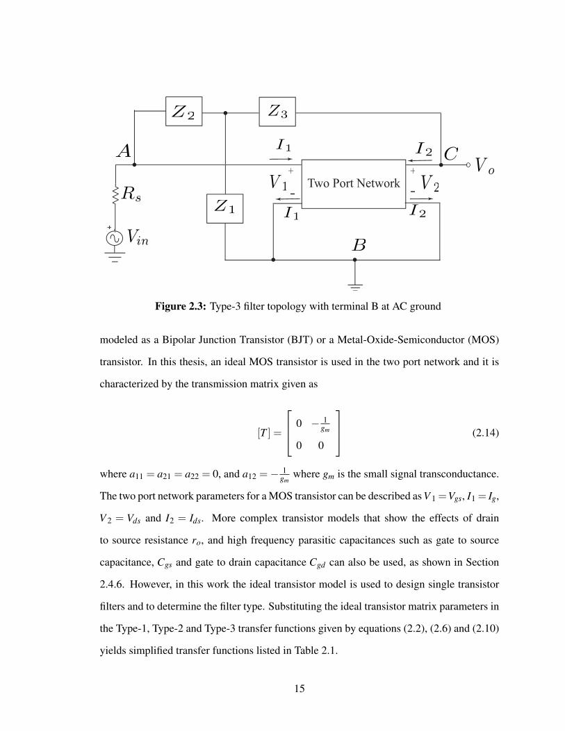
Finally, consider the Type-3 filter topology shown in Figure 2.3. This time, the input
and output are at terminals A and C, while terminal B is grounded. Nodal analysis of the
13

+
Two Port Network
Z2 Z3
V 2
I2
I1 I2Rs
V o
+
Z1
Vin
V 1 −
I1
+
−A
B
C
Figure 2.2: Type-2 filter structure with terminal C at AC ground
structure yields the following transfer function
H3 (s) =Vo
Vin=
Z1Z2 +Z1Z3 +Z2Z3 +a12Z1
413a11 +423a21 +433a22 +a12 (Rs +Z1 +Z2)−RsZ1(2.10)
where
413 = Rs (Z1−Za22 +Z3)+Z1Z2 +Z1Z3 +Z2Z3 (2.11)
423 = Rs (Z1Z2 +Z1Z3 +Z2Z3 +Z1a12) (2.12)
and
433 = Rs (Z1 +Z2) (2.13)
Since a single transistor active filter design is targeted, the two port network can be
14
+
Two Port Network
Z2 Z3
V 2
I2
I1 I2Rs
V o+
Z1
Vin
V 1−
I1
+
−A
B
C
Figure 2.3: Type-3 filter topology with terminal B at AC ground
modeled as a Bipolar Junction Transistor (BJT) or a Metal-Oxide-Semiconductor (MOS)
transistor. In this thesis, an ideal MOS transistor is used in the two port network and it is
characterized by the transmission matrix given as
[T ] =
0 − 1gm
0 0
(2.14)
where a11 = a21 = a22 = 0, and a12 =− 1gm
where gm is the small signal transconductance.
The two port network parameters for a MOS transistor can be described as V 1 =Vgs, I1 = Ig,
V 2 = Vds and I2 = Ids. More complex transistor models that show the effects of drain
to source resistance ro, and high frequency parasitic capacitances such as gate to source
capacitance, Cgs and gate to drain capacitance Cgd can also be used, as shown in Section
2.4.6. However, in this work the ideal transistor model is used to design single transistor
filters and to determine the filter type. Substituting the ideal transistor matrix parameters in
the Type-1, Type-2 and Type-3 transfer functions given by equations (2.2), (2.6) and (2.10)
yields simplified transfer functions listed in Table 2.1.
15

Topology Transfer Function
Type-1 H1 (s) =(Z1gm+Z3gm+1)Z2+Z1Z3gm
(Z1gm+1)Rs+Z1+Z2
Type-2 H2 (s) =(Z1gm+Z3gm)Z2+(Z1gm+1)Z3
(Z1gm+1)Rs+(Z1gm+Z3gm+1)Z2+(Z1gm+1)Z3
Type-3 H3 (s) =Z1−(Z1gm+Z3gm)Z2−Z1Z3gm
(Z1gm+1)Rs+Z1+Z2
Table 2.1: Type-1, Type-2 and Type-3 transfer functions using an ideal transistor
+
Two Port Network
Z2
Z3
V 2
I2
I1 I2Rs
V o
+
Z1
Vin
V 1−
I1
+
−
Figure 2.4: Altered Type-3 filter structure with Rs as an external resistor
2.2 Variation of Type-3 Filter Structure1
Consider the filter topology shown in Figure 2.4. It is a variation of the general Type-3 filter
structure given in Figure 2.3, obtained by exchanging the grounded terminal of Z1 and V in.
In this case, Rs is used as an external resistor rather than as an internal source resistance and
is connected to Z2 and the input terminal of the two port network. Once again by circuit
analysis, we find the transfer function of the new Type-3 filter topology to be
1Variations of Type-1 and Type-2 filter structures were attempted but did not yield any valid second orderfilters.
16

H3 (s) =Vo
Vin=
RsZ2a22 +RsZ3 +a12 (Rs +Z2)
41a11 +42a21 +43a22 +a12 (Rs +Z1 +Z2)−RsZ1(2.15)
where
413 = Rs (Z1−Za22 +Z3)+Z1Z2 +Z1Z3 +Z2Z3 (2.16)
423 = Rs (Z1Z2 +Z1Z3 +Z2Z3 +Z1a12) (2.17)
433 = Rs (Z1 +Z2) (2.18)
Substituting the ideal transistor matrix parameters (a11 = a21 = a22 = 0,a12 =− 1gm
) in the
transfer function given by equation (2.15) yields a simplified expression
H3 (s) =Vo
Vin=
Z2− (Z3gm−1)Rs
(Z1gm +1)Rs +Z1 +Z2(2.19)
2.3 All possible filter types
An exhaustive search for all possible three impedance single transistor second order filters
was performed in MAPLE for different impedance combinations of each filter topology.
The combinations of Z1,2,3 in the search code consist of no more than two resistors (ex-
cluding resistor Rs) and two storage elements (capacitors and inductors). The results of this
search was then compared to the second order transfer function
H (s) = KN (s)
s2 +Bs+ω2o
(2.20)
to determine the type of filter. For example, N(s) = ω2o gives a lowpass filter, N(s) = Bs
gives a bandpass filter, N(s) =s2 gives a highpass filter, N(s) =s2 +ω2o gives a bandstop
17

filter, N(s) =s2−Bs+ω2o gives an allpass filter and N(s) =s2 +B1s+ω2
o , where B1 6= B
gives a gain equalizer (GE). Gain K, pole frequency ωo, and quality factor Q expressions
are also found from MAPLE. All possible impedance combinations were considered and
the valid second order filters obtained from MAPLE for each filter topology are presented
in Tables 2.2, 2.3 , 2.4 and 2.5.
Note it is possible to obtain allpass filters from selected gain equalizer filters if they
fulfill the condition Q =−Qz, where Qz is the zero quality factor. For example, for the gain
equalizer filters #1 and #3 in Table 2.4, solving for Rs under the condition Q =−Qz yielded
Rs =R2 (1−gm (R2 +2R3))
R2gm (R3gm +1)+R3gm−1
which shows that the circuits work as allpass filters as long as gm (R2 +2R3)< 1. Similarly,
Rs for the gain equalizer filter #2 of Table 2.4 was obtained as
Rs =R1 (1−gm (R1 +2R3))
gm (R1 +R3)(R1gm +1)(2.21)
and the filter works as an allpass if gm (R1 +2R3) < 1. The gain equalizer filters #1 and
#3 in Table 2.5 was found to work as allpass filters and the expression of R3 under the
condition Q =−Qz was found to be
R3 =R1 (Rsgm +1)+2Rs
Rsgm(2.22)
2.4 Discussion of Selected Filters
In this section, full circuit implementations, biasing requirements2 and non-ideal effects of
selected filters are presented. Designs of different filter types such as bandpass, bandstop,
and allpass filters from Table 2.5 are shown. Input and output impedances of each circuit
2For most of the filters one DC current source suffice to bias the transistor. However, it was found thatsome filters require an extra biasing network, as discussed in Section 2.4.5.
18

TopologyZ1,2,3 Pole Frequency: ωo Quality Factor, Q ExtraFilter Gain, K Zero Quality Factor, Qz Biasing
Type-1
R1, L2 +C2, R31√
C2L2
(√L2C2
)1
R1Rsgm+R1+RsYes
GE R1gm +R3gm +1(√
L2C2
)R1gm+R3gm+1
R1R3gm
(#1)
L1 +C1, R2, R31√
C1L1
(√L1C1
)Rsgm+1R2+Rs
No
GE gm(R2+R3)Rsgm+1
(√L1C1
)gm(R2+R3)
R2(R3gm+1)(#2)
R1, L2 ‖C2, R31√
C2L2
(√C2L2
)R1Rsgm +R1 +Rs No
GE R1R3gmR1Rsgm+R1+Rs
(√C2L2
)R1R3gm
R1gm+R3gm+1
(#3)
L1 ‖C1, R2, R31√
C1L1
(√C1L1
)(R2+Rs)(Rsgm+1) No
GE R2(R3gm+1)(R2+R3)
(√C1L1
)R2(R3gm+1)gm(R2+R3)
(#4)
Table 2.2: All possible second order filters for Type-1 filter configuration
are also derived.
2.4.1 Bandpass Filter
The Type-3 bandpass filter #2 from Table 2.5 is designed as shown in Figure 2.5. One of
the three impedances is a series LC network and the other two impedances are resistors.
This can also be called a LC resonance based filter where the capacitor and inductor values
control the center or pole frequency. A DC current source Ib is connected from the drain of
the MOS transistor to the supply voltage V dd to ensure proper biasing. The expressions of
the design parameters Q, K and ωo are given in Table 2.5.
Since the bandpass filter is a resonance based filter it will have quality factor, Q > 12
which requires L1 > R2+Rs2(Rsgm+1)ωo
, resulting in complex poles. To obtain a characteristic
response of a second order bandpass filter, the general transfer function given by equation
19

TopologyZ1,2,3 Pole Frequency: ωo Quality Factor, Q ExtraFilter Gain, K Zero Quality Factor, Qz Biasing
R1, R2, L3 +C31√
C3L3
(√L3C3
)gm(R1+R2)+1
(R2+Rs)(R1gm+1) No
GE 1(√
L3C3
)gm(R1+R2)+1
R1R2gm
(#1)
R1, L2 +C2, R31√
C2L2
(√L2C2
)gm(R1+R3)+1
(R3+Rs)(R1gm+1) No
GE gm(R1+R3)gm(R1+R3)+1
(√L2C2
)gm(R1+R3)
R3(R1gm+1)(#2)
L1 +C1, R2, R31√
C1L1
(√L1C1
)gm(R2+Rs+R3)
R2+Rs+R3(R2gm+1) No
GE R2+R3R2+Rs+R3
(√L1C1
)gm(R2+R3)
R3(R2gm+1)(#3)
Type-2
R2, R3, L3 ‖C31√
C3L3
(√C3L3
)(R2+Rs)(R1gm+1)
gm(R1+R2)+1 No
GE R1R2gm(R2+Rs)(R1gm+1)
(√C3L3
)R1R2gm
gm(R1+R2)+1(#4)
R1, L2 ‖C2, R31√
C2L2
(√C2L2
)(R3+Rs)(R1gm+1)
gm(R1+R3)+1 No
GE R3Rs+R3
(√C2L2
)R3(R1gm+1)gm(R1+R3)
(#5)
L1 ‖C1, R2, R31√
C1L1
(√C1L1
)R2+Rs+R3(R2gm+1)
gm(R2+Rs+R3)No
GE R3(R2gm+1)R2+Rs+R3(R2gm+1)
(√C1L1
)R3(R2gm+1)gm(R2+R3)
(#6)
Table 2.3: All possible second order filters for Type-2 filter structure
(1.6) is plotted in MATLAB for a Q of 2.5, pole frequency, fo = 16.3 MHz and center
frequency gain K = 0.99. The magnitude and phase responses are shown in Figure 2.6.
The expression for the center frequency gain K given in Table 2.5 (filter #2) show that the
gain cannot be greater than 1 as it will lead to one of the resistors or gm becoming negative
which is not possible.
20

TopologyZ1,2,3 Pole Frequency: ωo Quality Factor, Q ExtraFilter Gain, K Zero Quality Factor, Qz Biasing
L1 +C1, R2, R31√
C1L1
(√L1C1
)(Rsgm+1)
R2+RsNo
Type-3
GE or AP 1−gm(R2+R3)(Rsgm+1)
(√L1C1
)gm(R2+R3)−1
R3R2gm
(#1)
R1, L2 ‖C2, R31√
C2L2
(√C2L2
)(Rs (gmR1 +1)+R1) No
GE or AP R1(1−R3gm)Rs(gmR1+1)+R1
(√C2L2
)R1(R3gm−1)gm(R1+R3)
(#2)
L1 ‖C1, R2, R31√
C1L1
(√C1L1
)R2+Rs
(Rsgm+1) No
GE or AP −R2R3gmR2+Rs
(√C1L1
)R2R3gm
gm(R2+R3)−1(#3)
Table 2.4: All possible second order filters for Type-3 filter structure
TopologyZ1,2,3 Pole Frequency: ωo Quality Factor, Q ExtraFilter Gain, K Zero Quality Factor, Qz Biasing
R1, L2 +C2, R31√
C2L2
(√L2C2
)1
R1Rsgm+R1+RsYes
GE or AP 1(√
L2C2
)1
Rs(1−R3gm)
(#1)
L1 +C1, R2, R31√
C1L1
(√L1C1
)Rsgm+1R2+Rs
No
Alternate Bandpass 1− R3RsgmR2+R3
-Type-3 (#2)Filter
R1, L2 ‖C2, R31√
C2L2
(√C2L2
)R1Rsgm +R1 +Rs No
GE or AP Rs(R3gm−1)R1Rsgm+R1+Rs
(√C2L2
)Rs (1−R3gm)
(#3)
L1 ‖C1, R2, R31√
C1L1
(√C1L1
)(R2+Rs)(Rsgm+1) No
Bandstop 1− R3RsgmR2+R3
-(#4)
Table 2.5: All possible filters of an altered Type-3 filter topology of Figure 2.4.
21

+
L1 C1
Rs
R2
R3
Ib
Vin
V o
M1
V dd
Figure 2.5: Second order bandpass filter using a single transistor
105
1010
−20
−10
0
Frequency (Hz)
Mag
nit
ud
e in
dB
105
1010
−100
0
100
Frequency (Hz)
Ph
ase
in D
egre
es
Figure 2.6: General bandpass filter transfer function plotted in MATLAB at fo = 16.3MHz, K = 0.99 and Q = 2.5
2.4.1.1 Input and Output impedance of Bandpass Filter
The expression of input impedance Zin of the second order bandpass filter found looking
into the circuit from the right of the source is given as
22

Zin (s) =s2C1L1(Rsgm +1)+ sC1(R2 +RS)+(Rsgm +1)
sC1(Rsgm +1)(2.23)
From the bandpass circuit in Figure 2.5 it is observed that the input impedance is very high
due to the series LC component used as Z1, where either the inductor or the capacitor will
simulate an open circuit at very high and low frequencies, respectively. At low frequencies,
Zin is reduced to 1/sC1 and at very high frequencies, it becomes sL1. Hence this circuit
will not be suitable for cascading multiple stages or adding a load stage without the use of
a unity gain buffer between them to prevent loading. At the resonance or pole frequency
the reactive components cancel each other, that is, Z1 gets shorted and the input impedance
is obtained as
Zin =R2 +Rs
Rsgm +1(2.24)
The output impedance of the bandpass circuit is obtained as
Zout (s) =s2C1L1(R2 +R3 +Rs)+ sC1R3(R2 +Rs)+(R2 +R3 +Rs)
s2C1L1(Rsgm +1)+ sC1(R2 +RS)+(Rsgm +1)(2.25)
At very high and low frequencies, Z1 acts as an open circuit and the equivalent circuit
diagram is shown in Figure 2.7. From straightforward circuit analysis, it can be shown
that Zout =(R2+R3+Rs)(Rsgm+1) . Whereas, at pole frequency, Z1 is shorted to ground due to the
reactances canceling each other and resulting in the circuit seeing an output impedance of
Zout = R3. The equivalent circuit diagram to find output impedance at the pole frequency
is shown in Figure 2.8.
In the initial circuit analysis of the alternate Type-3 filters, Rs was treated as an external
resistor and the internal resistance (Rin) of the source generator was ignored. To consider
any possible effect of Rin, the nodal equations and transfer function are adjusted. This
gives rise to altered Q and K expressions, which show the additional terms introduced by
23

Rs
R2
R3Io
V o
V g
Zout
gmVgs
Figure 2.7: Small signal diagram to find Zout at very high and low frequencies
Rs
R2
V g gmVgs
V o
Io
Zout
R3
Figure 2.8: Small signal diagram to find Zout at pole frequency
Rin in the denominator that will adversely affect the quality factor and DC gain. The pole
frequency, however, remains unchanged. Hence ideally Rin should be as small as possible
as it reduces Q and K as shown in equations 2.26 and 2.27, respectively,
Q =L1 (Rsgm +1)
√1
C1L1
R2 +Rs +Rin(Rsgm +1)(2.26)
K =R2 +Rs−R3Rsgm
R2 +Rs +Rin(Rsgm +1)(2.27)
As can be observed from circuit analysis, the input impedance at the pole frequency
due to Rin is Zin = Rin +R2+Rs
Rsgm+1 and the output impedance at the pole frequency becomes
Zout =Rin(R2+R3+Rs)+R3(R2+Rs)
Rin(Rsgm+1)+(R2+Rs).
24

+
Vin
L1
C1
R2
Rs
R3
V dd
M1
Ib
V o
Figure 2.9: Second order bandstop filter topology
2.4.2 Bandstop or Notch Filter
The Type-3 active bandstop filter #4 from Table 2.5 was designed as shown in Figure 2.9,
where one of the three impedances is a parallel LC network and the other two impedances
are resistors. Again the resonance frequency of the LC parallel network coincides with the
pole frequency of the notch filter. A current source Ib is used for biasing the transistor.
The expressions of the design parameters Q, K and ωo are given in Table 2.5. To
obtain a characteristic notch circuit response the second order notch transfer function given
by equation (1.9) is plotted in MATLAB. The magnitude and phase responses for Q = 2,
K = 0.99 and pole frequency f o = 16.3 MHz are shown in Figure 2.10. Similar to the
bandpass filter case, the DC gain K of the notch filter cannot be greater than unity, as either
the resistors or gm will become negative.
2.4.2.1 Input and Output Impedance of the Bandstop Filter
By circuit analysis, the expression of input impedance Zin of the second order notch filter
was found to be
25

105
106
107
108
109
−30
−20
−10
0
Frequency (Hz)
Mag
nit
ud
e in
dB
105
106
107
108
109
−100
0
100
Frequency (Hz)
Ph
ase
in D
egre
es
Figure 2.10: General bandstop filter transfer function plotted in MATLAB for fo = 16.3MHz, K = 0.99 and Q = 2
R3
R2
Rs
V g gmVgs
V oVin
Iin
Zin
Figure 2.11: Small signal diagram to find Zin of the notch circuit at very high frequencies
Zin (s) =s2C1L1(R2 +RS)+ sL1(Rsgm +1)+(R2 +RS)
(s2C1L1 +1)(Rsgm +1)(2.28)
To find the input impedance at very high frequencies, Z1 can be replaced by a short
circuit as the inductor acts as an open circuit and the capacitor gets shorted. The equivalent
bandstop filter is shown in Figure 2.11. By analyzing the circuit it is found that Zin at high
frequencies is expressed as Zin =R2+Rs
Rsgm+1 . This is also true for low frequencies where the
26

inductor is shorted and capacitor acts as an open circuit. At resonance frequency, however,
the input impedance approaches infinity because the inductive and capacitive reactances
equal each other and the LC tank circuit is replaced by an open circuit, thus presenting a
high impedance to a narrow range of frequencies.
Output impedance is found to be Zout = R3 at low and high frequencies, where the
signal source is set to zero (V in=0) and Z1 is connected to ground. The equivalent circuit
diagram is the same as the one shown in Figure 2.8 but in this case for high frequencies.
Consider the circuit in Figure 2.7 to find output impedance of the notch filter at resonance
frequency. The output impedance expression is found to be Zout =(R2+R3+Rs)(Rsgm+1) at resonance
frequency, where the Z1 branch is replaced with an open circuit.
To consider the effect of signal source resistance Rin for the notch circuit the nodal
equations are adjusted to include Rin resulting in new expression for transfer function. New
expressions of Q and K due to Rin are found to be
Q =C1
√1
C1L1
Rin (Rsgm +1)+Rs +R2
Rsgm +1(2.29)
K =R2 +Rs−R3Rsgm
R2 +Rs +Rin(Rsgm +1)(2.30)
Input impedance due to Rin is Zin = Rin+R2+Rs
Rsgm+1 at low and high frequencies and output
impedance is Zout =Rin(R2+R3+Rs)+R3(R2+Rs)
Rin(Rsgm+1)+(R2+Rs). As expected output impedance at resonance
frequency is not affected by Rin as the entire branch with Z1 becomes an open circuit.
2.4.3 Allpass Filter
The Type-3 allpass filter #3 from Table 2.5 is designed as shown in Figure 2.12, which
employs a parallel LC network as Z2 and two resistors as Z1 and Z3. This can also be called
a LC resonance based filter where the capacitor and inductor values control the resonance
or pole frequency. The expressions of design parameters ωo, Q, Qz (zero quality factor)
27

L2C2
R1 R3
Rs
+
Vin
V dd
Ib
V o
M1
Figure 2.12: Second order AP filter structure
and K are given in Table 2.5.
A general transfer function of an allpass filter given as
H (s) =Vo
Vin(s) = K
(s2− ωo
QZs+ω2
z
)(
s2 + ωoQ s+ω2
o
) (2.31)
was plotted in MATLAB. The magnitude and phase responses for Q = |Qz|= 1, K = 1, and
f o = 16.3 MHz are shown in Figure 2.13.
2.4.3.1 Input and Output Impedance of the Allpass Filter
At high frequencies C2 gets shorted and L2 becomes an open circuit, whereas, the opposite
is true for low frequencies, where the capacitor is open and the inductor is shorted. In both
cases, Z2 can be replaced as a short circuit. The equivalent circuit diagram to find input
impedance is shown in Figure 2.14. By circuit analysis, it can be shown that at low and high
28

105
106
107
108
109
−30
−20
−10
0
Frequency (Hz)
Mag
nit
ud
e in
dB
105
106
107
108
109
−100
0
100
Frequency (Hz)
Ph
ase
in D
egre
es
Figure 2.13: General allpass filter transfer function plotted in MATLAB for fo = 16.3MHz, K = 1 and Q = |Qz|= 1
frequencies, Zin =R1(Rsgm+1)+Rs
(Rsgm+1) . At pole frequency, input impedance approaches infinity
as L2 and C2 resonate with each other and is replaced by an open circuit. To find the output
impedance, the input voltage is set to zero that connects R1 to ground. From circuit analysis
the output impedance is found to be Zout = R1 +R3 at the pole frequency where Z2 is an
open circuit. At very high and low frequencies, it becomes Zout =R2
3R3+(R1||Rs||R3)(gmR3−1)
where Z2 is shorted as illustrated in Figure 2.15.
2.4.4 Effect of gm
From the expressions of design parameters K, Q and ωo of the Type-3 filters shown in Table
2.5, it can be noted that gm has no effect on the pole frequency but will affect the DC gain
and quality factor. The component gm can be controlled using the biasing current source
or to a less extent by the W/L ratio of the transistor. For the bandpass filter #2, raising gm
will improve Q but will lower center frequency gain K. For the notch filter #4, the design
equations show that increase in gm will lower both Q and DC gain K. These aspects have
29

Vin
Iin
Zin
Rs
R3V o
gmVgs
V gR1
Figure 2.14: Allpass filter equivalent small signal diagram to find input impedance Zin atvery high frequencies
Rs
V g R3
gmVgs
V oIo
Zout
R1
Figure 2.15: Allpass filter equivalent small signal diagram to find output impedance Zoutat high frequencies
to be carefully considered while carrying out simulations or experimental measurements
and component values need to be chosen accordingly to obtain results that are close to the
theoretical ones.
2.4.5 Biasing Details
For accurate implementation of single MOS transistor filters, care should be taken to main-
tain the transistors at saturation mode of operation, for which the conditions V gs>V th and
V ds>V gs−Vth have to be met. Some impedance combinations can lead to the MOS transis-
tor going out of saturation mode. For example, the Type-3 allpass filter #1 shown in Table
2.5 uses a series LC network for Z2 that puts the transistor at improper operation mode as
30

L2
C2
R1 R3
Rs
+
Vin
V dd
V o
M1
V dd
Ib2Ib1
Figure 2.16: Allpass filter #1 from Table 2.5 implemented with an additional DC biasingcurrent source
the capacitor blocks DC voltage to the gate terminal of the transistor. Similarly, the Type-1
gain equalizer filter #1 given in Table 2.2 also puts the transistor out of saturation mode
due to the use of series LC network as Z2. However, these circuits can be made to operate
by use of extra biasing. For example, Figure 2.16 shows the Type-3 allpass filter #1 from
Table 2.5 with an extra DC current source Ib2 connected to the gate terminal of the MOS
transistor. To check the validity of the circuit it was simulated in Cadence Spectre using a
single transistor with aspect ratio W/L= 6µm/0.2µm and operated from a supply of 1.5 V
in IBM 0.13 µm CMOS process. The allpass filter was designed to operate at fo = 4.6 MHz
with component values set to L2= 24 µH, C2= 50 pF, R1= 50 Ω, R3=930 Ω and Rs= 500
Ω. The simulated magnitude and phase responses are shown in Figure 2.17. It is observed
that the simulated DC gain is -0.69 dB which is close to the theoretical -0.1 dB gain. The
transient waveforms of the input and output signals at pole frequency 4.6 MHz is shown in
Figure 2.18.
31

Figure 2.17: Simulated magnitude and phase responses of allpass filter of Figure 2.16
2.4.6 Non-ideal Effects
2.4.6.1 Effect of ro
So far the MOS transistor was assumed to be ideal, by neglecting the drain to source re-
sistance ro and intrinsic parasitic capacitances of the transistor. In this section, the non-
idealities of the proposed general circuit are discussed. To analyze the effects of ro, the
transistor can be modeled by an alternate transmission matrix given by
[T ] =
− 1gmro
− 1gm
0 0
(2.32)
32

Figure 2.18: Simulated input and output waveforms of allpass filter of Figure 2.16 at polefrequency of 4.6 MHz
Bandpass filter (Table 2.5, #2)
The matrix given by equation (2.32) changes the transfer function of the bandpass filter
and yields new expressions for Q and K. The pole frequency expression and order of the
bandpass filter remains same. That is,
Q =
√L1
C1
ro(Rsgm +1)+R2 +R3 +Rs
ro(R2 +Rs)+R3(R2 +Rs)(2.33)
and
33

K =ro(R2 +Rs−R3Rsgm)
ro(R2 +Rs)+R3(R2 +Rs)(2.34)
The input and output impedance of the circuit due to ro can also be considered. The
input impedance at pole frequency becomes Zin =(R2+Rs)ro+R2R3+R3Rs(Rsgm+1)ro+R2+R3+Rs
, while at very high
and low frequencies the circuit sees sL1 and 1/sC1 respectively, as can be observed from
the circuit diagram in Figure 2.5. As expected, the effective output impedance seen looking
into the drain terminal of the transistor is Zout = ro ‖ R3 at the pole frequency, whereas,
at low and high frequencies Zout =ro(R2+R3+Rs)
ro(Rsgm+1)+R2+R3+RS, when Z1 is replaced by an open
circuit.
Bandstop filter (Table 2.5, #4)
For the bandstop circuit, ro alters the transfer function and hence the Q and K expressions
become
Q =
√C1
L1
ro(R2 +Rs)+R3(R2 +Rs)
ro(Rsgm +1)+R2 +R3 +Rs(2.35)
K =ro(R2 +Rs−R3Rsgm)
ro(R2 +Rs)+R3(R2 +Rs)(2.36)
Input and output impedance of the bandstop filter considering the affect of ro is found to be
Zin =(R2+Rs)ro+R2R3+R3Rs(Rsgm+1)ro+R2+R3+Rs
and Zout = ro‖R3 at low and high frequencies where Z1 acts as
a short circuit. At resonance frequency, Zout =ro(R2+R3+Rs)
ro(Rsgm+1)+R2+R3+RS, where Z1 is an open
circuit. As expected, ro has no effect on the pole location and the filter order remains same.
In the next section, however, it is shown that parasitic capacitances change the order of the
filter by adding extra poles and zeroes.
34

2.4.6.2 Effect of parasitic capacitances
At very high frequencies the effects of parasitics are prominent which affects the expected
performance of a filter. To consider the effects of high frequency parasitic capacitances,
more complex transistor models are used.
First, to analyze the effect of Cgs, the transistor model given by
[T ] =
− 1rogm
− 1gm
− sCgsrogm
− sCgsgm
(2.37)
is used to derive the transfer function and the pole and zero locations. Cgs is connected
between the gate and source terminal of the transistor and hence shorts the gate to source
path at very high frequencies. Another effect of Cgs is that it adds an extra real pole and
zero which converts the second order bandpass filter to a third order filter. The additional
pole and zero due to Cgs is given by
ωz1 =RsR3gm−R2−Rs
CgsR2Rs(2.38)
ωp1 =
√ro(Rsgm +1)+R2 +R3 +Rs
CgsRs (R2 +R3 + ro)(2.39)
A similar effect is observed for the bandstop filter where the extra pole and zero due to Cgs
is found to be
ωz1 =RsR3gm−R2−Rs
CgsR2Rs(2.40)
ωp1 =
√R2 +Rs
CgsR2Rs(2.41)
Next we consider the effect of the parasitic capacitor Cgd on the bandpass circuit. It is
connected across the gate and drain terminals of the transistor and will get shorted at very
35

high frequencies, reducing the output impedance of the bandpass filter to Rs. It also adds
another pole and zero to the bandpass transfer function which are given by
ωz2 =RsR3gm−R2−Rs
CgdRs (R2 +R3)(2.42)
ωp2 =
√ro(Rsgm +1)+R2 +R3 +Rs
Cgd (R2 +R3)(Rsgmro + ro +Rs)(2.43)
In the case of bandstop filter the additional pole and zero due to Cgd are
ωz2 =RsR3gm−R2−Rs
CgdRs (R2 +R3)(2.44)
ωp2 =
√(R2 +Rs)(R3 + ro)
Cgd (R2R3Rs (gmro +1)+ ro (R2R3 +R2Rs +R3Rs))(2.45)
It is observed that both Cgs and Cgd add an extra real pole and zero converting the filter
from second to fourth order. This can be shown by using a more complex transmission
matrix (2.46) that yields a transfer function of the fourth order.
[T ] =
sCgd+1/rosCgd−gm
1sCgd−gm
s(sCgdCgsro+Cgdgmro+Cgd+Cgs)ro(sCgd−gm)
s(Cgd+Cgs)sCgd−gm
(2.46)
Hence, the filters do not work as expected beyond a certain frequency due to the high
frequency effects of the transistors. The frequencies at which these additional poles/ zeroes
occur can be found from the derived frequency expressions.
36

CHAPTER 3
Simulation and Experimental Results
To validate the theoretical study, simulation and experimental results of selected filters
are presented. The circuits were simulated in an IBM 0.13 µm CMOS process using the
Spectre simulation tool in Cadence design environment. Note that for Cadence simulations,
the filters were designed to operate at high frequencies (in the tens of MHz) as we intended
to implement one of the proposed filters in IC form. However, it was not possible to present
an IC chip in this work due to time constraints. The filters were verified experimentally
using standard discrete components connected on a breadboard and the measured responses
were observed from Network Analyzer HP4395A. For experimental testing the operating
frequency of the filters was lowered to the kHz range.
3.1 Bandpass Filter
The bandpass filter shown in Figure 2.5 was simulated using a single transistor with an
aspect ratio of W/L= 0.48 µm/0.18 µm and operated from a supply of 1.5 V. The component
values were found using the equations of Q, ωo, and K to be L1= 50 µH, C1= 1.9 pF, R2=1.2
kΩ, R3=100 Ω and Rs= 900 Ω. A bias current source of 400 µA yielded a center frequency
gain of -0.042 dB at 16.3 MHz for a Q of 2.5. The simulated results are shown in Figure
3.1, which is similar to the calculated gain of -0.08 dB at center frequency of 16.3 MHz.
Transient analysis of the bandpass filter was carried out at the center frequency of 16.3
MHz. The input signal and its corresponding output are shown in Figure 3.2, which shows
that the waveforms have equal amplitude at the pole frequency. This is expected because
37

Figure 3.1: Magnitude response of proposed bandpass filter simulated in Cadence tovalues of L1= 50 µH, C1= 1.9 pF, R2=1.2 kΩ, R3=100 Ω, and Rs= 900 Ω.
the simulated magnitude response in Figure 3.1 shows that the center frequency gain is
around 0 dB, that is, input and output signals have the same amplitude.
The bandpass filter was also tested experimentally using discrete components and CD4007
transistor arrays that operated from a 5 V supply. Component values used were C1 = 680
pF, L1 = 10 mH, Rs = 900 Ω, R2 = 1.2 kΩ and R3 = 100 Ω that resulted in a calculated pole
frequency of 61 kHz with a gain of -0.91 dB and Q = 7. The measured response shown
in Figure 3.3 had a pole frequency of 63.4 kHz where the gain is -1.286 dB and Q = 7.86.
To verify the experimental results, we tested the bandpass filter in PSPICE using CD4007
transistor model that operated from a 5 V supply. Component values of resistors, capacitor
and inductor were kept same as the experimental setup which resulted in a pole frequency
38

Figure 3.2: Cadence simulated transient responses of input and output signals ofbandpass filter at pole frequency of 16.3 MHz to values L1= 50 µH, C1= 1.9 pF, R2= 1.2
kΩ, R3=100 Ω and Rs= 900 Ω.
of 61.19 kHz with a gain of -1.30 dB and Q = 8.2. The simulated results from PSPICE
are shown in Figure 3.4. It is observed that the values of the design parameters (gain, qual-
ity factor and pole frequency) obtained from experimental measurements are very close to
those of the PSPICE simulations and the minor differences are due to the tolerances of the
discrete components used. Note that the center frequency gain K of the bandpass filter can
be made to move closer to unity gain (0 dB) but at the expense of quality factor Q. This is
because of some common terms that appear in both K and Q expressions (Table 2.5). For
example, raising the value of R2 will improve K but lower Q.
39

Figure 3.3: Measured magnitude response of bandpass filter to values of C1 = 680 pF,L1 = 10 mH, Rs = 900 Ω, R2 = 1.2 kΩ and R3 = 100 Ω.
3.2 Bandstop Filter
The bandstop circuit shown in Figure 2.9 was simulated in Cadence. It employed a single
transistor with an aspect ratio of W/L= 0.48 µm/0.18 µm and operated from a supply of 1.5
V. The parallel LC network used component values L1=10 µH, C1= 9.52 pF. The values of
the resistors used were R2= 600 Ω, R3=110 Ω, and Rs= 1.2 kΩ. A bias current source of 700
µA and gm = 73.8µA/V yielded a simulated DC gain of -0.05 dB and a notch frequency of
16.2 MHz which is in good agreement to the calculated notch frequency of 16.3 MHz and
DC gain of -0.06 dB. The notch depth at the center frequency 16.2 MHz was observed to be
-34.69 dB. Figure 3.5 shows the simulated magnitude response for the circuit. The transient
waveforms of the input and output signals at pole frequency 16.2 MHz are given in Figure
40

Figure 3.4: Magnitude response of bandpass filter simulated in PSPICE to values ofC1 = 680 pF, L1 = 10 mH, Rs = 900 Ω, R2 = 1.2 kΩ and R3 = 100 Ω.
3.6. It is observed that at the notch frequency the output signal is much smaller compared
to the input signal. This is because the notch frequency magnitude of the bandstop filter
was found to be -34.68 dB as shown in Figure 3.5.
To validate the bandstop filter, it was also tested experimentally using discrete compo-
nents and CD4007 transistor arrays. The circuit operated from a 5 V supply with compo-
nent values set to C1 = 68 pF, L1 = 2 mH, Rs = 1.2 kΩ, R2 = 500 Ω and R3 = 100 Ω that
yielded a calculated pole frequency of 432 kHz with a DC gain of -0.1 dB. The measured
magnitude response shown in Figure 3.7 has a notch at measured pole frequency of 425
kHz with a notch depth of -36.4 dB, while the DC gain is 0 dB. To check the accuracy of
the measured results, the bandstop filter was simulated in PSPICE using CD4007 transistor
and passive components that operated from a 5 V supply. Component values of resistors,
capacitor and inductor were kept same as the experimental setup. The simulated results are
41

Figure 3.5: Bandstop filter magnitude response simulated in Cadence to values of L1= 10µH, C1= 9.52 pF, R2= 600 Ω, R3=110 Ω, and Rs= 1.2 kΩ.
shown in Figure 3.8. It can be observed that the simulation results are in good agreement
with the experimental ones. The DC gain is around 0 dB for both cases and the measured
notch frequency of 425 kHz is close to the simulated value of 430 kHz. The measured
quality factor Q = 5.3 is close to simulated Q = 5.9. The slight discrepancies are attributed
to the tolerances and quality factors of the real components.
3.3 Allpass Filter
The allpass circuit shown in Figure 2.12 was simulated in Cadence. The filter was designed
to operate at 4.6 MHz with L2= 24 µH, C2= 50 pF, R1= 50 Ω, R3=930 Ω and Rs= 500 Ω
from a 1.5 V supply voltage. A bias current source of 600 µA yielded a DC gain of -0.7
dB, quite close to the theoretical DC gain of -0.1 dB at a calculated pole frequency of 4.6
MHz. Figure 3.9 shows the simulated magnitude and phase responses while Figure 3.10
42

Figure 3.6: Cadence simulated input and output waveforms of bandstop filter at the polefrequency of 16.2 MHz to values L1= 10 µH, C1= 9.52 pF, R2= 600 Ω, R3=110 Ω, and
Rs= 1.2 kΩ.
shows the transient waveforms at 4.6 MHz.
The allpass filter was also tested experimentally. The circuit operated from a 5 V supply
with component values set to C1 = 68 pF, L1 = 2 mH, R1 = 1 kΩ, R3 = 1.2 kΩ and Rs = 3.3
kΩ, designed to operate at 400 kHz. The measured magnitude and phase responses are
shown in Figure 3.11. To verify the measured results, the allpass filter was simulated in
PSPICE using CD4007 transistor and passive components of same values that operated
from a 5 V supply. The simulated results are shown in Figure 3.12. It can be observed that
the simulation results are close to the experimental ones.
43

Figure 3.7: Measured magnitude response of bandstop filter to values of C1 = 68 pF,L1 = 2 mH, Rs = 1.2 kΩ, R2 = 500 Ω and R3 = 100 Ω with a vertical scale of 5 dB/
division and a logarithmic horizontal scale where each cycle represents a factor of 10.
44

Figure 3.8: Magnitude response of bandstop filter simulated in PSPICE to values ofC1 = 68 pF, L1 = 2 mH, Rs = 1.2 kΩ, R2 = 500 Ω and R3 = 100 Ω.
45

Figure 3.9: Allpass filter magnitude and phase response simulated in Cadence to valuesL2= 24 µH, C2= 50 pF, R1= 50 Ω, R3=930 Ω and Rs= 500 Ω.
46

Figure 3.10: Cadence simulated input and output waveforms of allpass filter at polefrequency to values L2= 24 µH, C2= 50 pF, R1= 50 Ω, R3=930 Ω and Rs= 500 Ω.
47

Figure 3.11: Measured magnitude and phase response of allpass filter to values C1 = 68pF, L1 = 2 mH, R1 = 1 kΩ, R3 = 1.2 kΩ and Rs = 3.3 kΩ.
48

Figure 3.12: Magnitude response of allpass filter simulated in PSPICE to values ofC1 = 68 pF, L1 = 2 mH, R1 = 1 kΩ, R3 = 1.2 kΩ and Rs = 3.3 kΩ.
49

CHAPTER 4
A Fourth Order Chebyshev Filter
4.1 Classical Chebyshev Filter Design Approach
It is known that ideal analog brick wall filters are not practically realizable. Different
methods of approximations are used to design a filter that will satisfy certain desirable
conditions. Several filter approximations have been proposed in the past, such as But-
terworth, Chebyshev, Inverse Chebyshev, Elliptic and Bessel-Thompson, each having a
different output response. The choice of the approximation method to be used depends on
the filter specifications. The Butterworth, also referred to as a maximally flat magnitude
filter has a flat response in the passband and an adequate roll-off. The Chebyshev imple-
mentation has a steeper roll-off but has ripples in the passband. It is sometimes known as
the Type I Chebyshev filter. Inverse Chebyshev or Type II Chebyshev filters have ripples
in the stopband.
In classical filter methods, design of Chebyshev and other filter approximations is based
on equations and tables of theoretical values. For a given set of specifications, a lowpass
Chebyshev filter is normalized at a passband edge frequency of ωc = 1 rad/s and the order
of the filter is found from a given formula. Next, a set of formula or tabulated values are
used to find the poles and zeroes. Other types of filters such as bandpass, bandstop, high-
pass filters can be obtained by use of frequency transformations. For example, to design a
highpass Chebyshev filter, a lowpass prototype (LPP) is obtained by means of highpass to
lowpass frequency transformation. Then, the order, poles and zeroes and transfer function
of the LPP is found. Next, denormalization of the LPP transfer function and application of
50

+
Vin
L1 C1 R3
R2
Rs
V dd
M1
V dd
V o
Ib1
Ib2
V 2
Ib1
Rs
C2L2
V 1 M3
R5
R4
M2
V dd
Figure 4.1: Proposed Chebyshev fourth order bandpass filter
the lowpass to highpass inverse transformation is performed to obtain the high pass transfer
function that meets the given specifications. The final realization of the active filters can be
implemented using multiple operational amplifiers, OTAs or CCIIs, especially for higher
order filter structures where several passive and active elements are required. An applica-
tion of a Chebyshev filter was found in [31]. It used a passive bandpass Chebyshev filter to
achieve a wideband input match from 3.1 to 10 GHz for a low noise amplifier.
4.2 Proposed Fourth Order Chebyshev Filter
In this section, a fourth order active Chebyshev bandpass filter topology is introduced that
is based on the single transistor bandpass filter. The core of the circuit is shown in Figure
4.1. It can be observed that the classical fourth order passive Chebyshev bandpass filter
shown in Figure 4.2 is simpler compared to the proposed topology. However, classical
active higher order filters use at least one opamp and some passive elements. For example,
the third order active Chebyshev filter designed in [32] used two opamps and a couple of
passive elements. The proposed topology implementing a fourth order Chebyshev filter
using three transistors and several passive elements is shown in Figure 4.1.
The proposed circuit can be easily tuned as each stage controls only one pole which
51

Rs
L1 V o
C2L2
C1Vin
+
−
+
−RL
Figure 4.2: Passive fourth order bandpass filter
Design Parameters Stage 1 Stage 2
Pole frequency ωo1 =√
1C1L1
ωo2 =√
1C2L2
Quality factor Q1 =(Rsgm1+1)
√L1C1
R2+RsQ2 =
(Rsgm2+1)√
L2C2
R4+Rs
Gain K1 =R2+Rs−R3Rsgm1
R2+RsK2 =
R4+Rs−R5Rsgm2R4+Rs
Table 4.1: Chebyshev filter design equations for two stages
depends solely on the series LC network of that stage. The design parameters of each stage
of the Chebyshev filter is shown in Table 4.1. A Chebyshev filter with maximum passband
loss (ripple magnitude) of 2 dB and minimum stopband loss of 20 dB with pole frequencies
at 17 MHz and 29 MHz and a center frequency of 22.5 MHz at a Q of 3.6 was targeted.
The general transfer function of the fourth order Chebyshev filter is given by
Vo
Vin= K1K2
(ωo1Q
)s×(
ωo2Q
)s(
s2 +ωo1Q s+ω2
o1
)(s2 +
ωo2Q s+ω2
o2
) (4.1)
where K1, K2 are the gains and ωo1 , ωo2 represent the pole frequencies of the first and
second stages, respectively. In order to achieve a Type I Chebyshev filter response with
ripples in the passband, the first and second stages were designed such that they have the
same gain (K1 = K2) and quality factor Q but at different pole frequencies. The bandpass
filter design equations were used to calculate component values for each stage for a Q of
3.6 and unity gain at two different pole frequencies, which is solely controlled by L and
52

Vin
V dd
V o
Ib
M3
Figure 4.3: Source follower used as a voltage buffer
C. A unity gain voltage buffer was used between the two stages to prevent loading due to
impedance mismatch. The buffer circuit was implemented using a source follower.
Figure 4.3 shows a source follower structure, which was realized using a CMOS tran-
sistor M3. This is also referred to as a common drain amplifier as the input and output
signals are at the gate and source terminals, respectively while the drain terminal is at AC
ground. A current source Ib is used as the active load at the source terminal to provide
biasing to the MOS transistor. An alternative way of realizing the source follower is to use
a current mirror as an active load [33]. The primary purpose of using a buffer between the
two stages is to provide isolation between the two stages and prevent the second stage from
loading the first stage of the circuit due to impedance differences between the output node
of the first stage and input node of the second stage. Ideally, a source follower should have
very high input impedance so that the input node draws minimum current from the source
and does not load it. Also it must have very low output impedance so that it can drive the
53
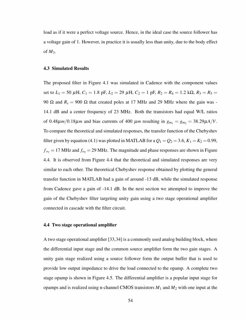
load as if it were a perfect voltage source. Hence, in the ideal case the source follower has
a voltage gain of 1. However, in practice it is usually less than unity, due to the body effect
of M3.
4.3 Simulated Results
The proposed filter in Figure 4.1 was simulated in Cadence with the component values
set to L1 = 50 µH, C1 = 1.8 pF, L2 = 29 µH, C2 = 1 pF, R2 = R4 = 1.2 kΩ, R3 = R5 =
90 Ω and Rs = 900 Ω that created poles at 17 MHz and 29 MHz where the gain was -
14.1 dB and a center frequency of 23 MHz. Both the transistors had equal W/L ratios
of 0.48µm/0.18µm and bias currents of 400 µm resulting in gm1 = gm2 = 38.29µA/V .
To compare the theoretical and simulated responses, the transfer function of the Chebyshev
filter given by equation (4.1) was plotted in MATLAB for a Q1 =Q2 = 3.6, K1 =K2 = 0.99,
f o1 = 17 MHz and fo2 = 29 MHz. The magnitude and phase responses are shown in Figure
4.4. It is observed from Figure 4.4 that the theoretical and simulated responses are very
similar to each other. The theoretical Chebyshev response obtained by plotting the general
transfer function in MATLAB had a gain of around -13 dB, while the simulated response
from Cadence gave a gain of -14.1 dB. In the next section we attempted to improve the
gain of the Chebyshev filter targeting unity gain using a two stage operational amplifier
connected in cascade with the filter circuit.
4.4 Two stage operational amplifier
A two stage operational amplifier [33,34] is a commonly used analog building block, where
the differential input stage and the common source amplifier form the two gain stages. A
unity gain stage realized using a source follower form the output buffer that is used to
provide low output impedance to drive the load connected to the opamp. A complete two
stage opamp is shown in Figure 4.5. The differential amplifier is a popular input stage for
opamps and is realized using n-channel CMOS transistors M1 and M2 with one input at the
54

105
1010
−30
−20
−10
Frequency (Hz)
Mag
nit
ude
in d
B
105
1010
−100
0
100
Frequency (Hz)
Phas
e in
Deg
rees
Figure 4.4: Comparison between ideal (dashed line) and simulated (solid line) magnitudeand phase responses of Chebyshev filter
non-inverting and the second input at the inverting terminal. The transistors have identical
sizes and are biased at the same DC voltage. The output voltage of a differential amplifier
can be expressed as
vout = ADM (v1− v2)±ACM
(v1 + v2
2
)(4.2)
where ADM and ACM are the differential and common mode voltage gains, respectively.
The purpose of the differential amplifier is to amplify the difference between the two input
signals and suppress the common voltage at the inputs. Thus, an ideal differential ampli-
fier should have zero common mode voltage gain or infinite common mode rejection ratio
(CMRR), which is the ratio of differential to common mode gain. The biasing circuitry con-
sists of a current source Ib and a diode connected transistor M8 which forms current mirror
55

M2
M5
M3 M4 M6
M7M8
M1
Ib
V dd
Vin
V o
Vin
V 1
+
CcRc
I5
CL
Figure 4.5: Two stage operational amplifier [33, 34]
with n-channel transistors M5 and M7. The transistor M5 acts as a tail current source. Ib
provides a DC gate voltage to M5 generating a current sink I5 that biases M1 and M2. The
gate terminal of M5 is at ac ground and the resistance of the tail current source is the re-
sistance seen into the drain of M5, which is rds5 . Ideally a tail current source should have
infinite resistance so that common mode rejection ratio (CMRR) is infinite. The higher the
resistance of the tail current source, the lower will be the common mode gain, resulting in
better common mode rejection ratio for the differential amplifier. Transistors M3 and M4 of
p-channel type form a current mirror active load connected between the drains of M1 and
M2 and the power supply V dd . Therefore, the current flowing through M3 is mirrored onto
transistor M4 by virtue of the transistors having matched properties and the gate terminals
tied together resulting in same gate to source voltage (V gs). This guarantees the same drain
56

gm6Vgs6 rds6 ‖ rds7
Vg6V 1 V o
Figure 4.6: Small signal diagram of a common source amplifier
currents I5/2 flowing through the two branches, that adds up to I5, the current in the tail cur-
rent sink M5. The current mirror topology converts the differential input signal to a single
ended output signal. Since the input and output signals are currents, an ideal current mir-
ror will have zero input resistance and infinite output resistance. However, for real current
mirrors, the input resistance is determined by the diode connected transistor M3 and can be
shown to be (1/gm3) ‖ rds3 ≈ (1/gm3) for rds3 1/gm3 . The output resistance of the current
mirror seen looking into the drain terminal of M4 is rds4 , which is large enough to provide
a good voltage gain. The gain of the first stage is derived to be Av1 = gm1 (rds2 ‖ rds4).
The second stage is a common source gain stage that is included to provide additional
gain. Here, transistor M6 serves as the p-channel common source amplifier along with M7
as the active load. The gain of the second stage is given by Av2 = gm6
(rds6 ‖ rds7
)which is
obtained from the small signal model of the common source amplifier as shown in Figure
4.6.
4.4.1 Slew Rate
The slew rate (SR) is the maximum rate of change of opamp output voltage. In the case of
a differential amplifier when there is a large input signal, SR is determined by the current
flowing through compensation capacitance CC. When input voltage at the non-inverting
terminal is maximum such that M1 is off, M2 is on and the current mirror pair M3, M4 is
57

off, the bias current I5 will flow from CC. Conversely, when input voltage at the inverting
terminal is maximum, M2 is off and the bias current I5 flows through M1 and the current
mirror pair M3, M4 into the compensation capacitor CC. In both cases, the maximum
current entering or leaving CC is I5 yielding SR = I5CC
.
4.4.2 Compensation of the two stage operational amplifier
It is known that the stability of an amplifier can be checked from the frequency and phase
responses of the amplifier. A minimum phase margin of 45º is required to ensure stability,
while 60º is usually preferred to avoid ringing effect of output signals [33, 34]. First order
systems have one pole and hence is unconditionally stable with a phase margin close to
90º. However, second order systems have two poles that cause a negative phase shift of 90º
for each pole and can lead to a poor phase margin depending on the positions of the poles
and unity gain frequency. Hence, the Miller compensation technique is used to modify the
phase margin to a desired value to keep the second order system stable. In this method, a
compensation capacitor CC is connected from the output of first stage to the input of the
second stage.
The differential stage has a pole located at ωp1 =1
R1C1, where R1 = rds2 ‖ rds4 is the
resistance seen from the output of the differential stage and C1 is the capacitance seen from
the output of the differential stage. Due to Miller effect, the effective capacitance connected
in parallel to R1 increases to CC (1+A) where A is the gain from V 1 to V out , causing the
first pole to move to a much lower frequency. Also, the compensation capacitor causes the
second pole shift to a higher frequency, preferably more than the unity gain frequency. The
overall objective of the Miller compensation is to reduce the frequency of one dominant
pole to make it much lower relative to the other poles and zeroes, causing the second order
system frequency response to be similar to that of a first order system. From the transfer
function [33] of the two stage opamp, it is seen that in addition to two poles, there is also
a zero present in the right half plane that produces a negative phase shift, degrading the
58

Vin
V o
C1gm1Vin rds2 ‖ rds4
Rc Cc
gm6V1 rds6 ‖ rds7 C2
V 1
+
−
Figure 4.7: Small signal model of two stage operational amplifier
stability of the system. Hence to remedy the situation a nulling resistor RC is introduced.
Different methods of controlling RHP zero using RC is mentioned in [33,34]. For this case,
RC is chosen such that it cancels out the zero. The small signal diagram of the two stage
opamp is shown in Figure 4.7. The poles and zeroes found from the transfer function are
as follows
ωp1 =1
gm6R1R2CC(4.3)
ωp2 =gm6
C2(4.4)
ωz =−1
CC (1/gm6−RC)(4.5)
where R2 = rds6 ‖ rds7 is the output resistance of the second stage and C2 is the output
capacitance of the second stage.
4.5 Chebyshev filter cascaded with two stage operational amplifier
Since the pole frequencies of the Chebyshev filter are at 17 MHz and 29 MHz, the gain
bandwidth product of the opamp was designed to be at 530 MHz, as beyond the unity gain
bandwidth the Chebyshev gain gets even lower than the original. The designed opamp had
a gain of 31 dB and phase margin of 56º. Note that it is possible to improve the gain of
59

Figure 4.8: Magnitude and phase response of two stage operational amplifier simulated inCadence
the opamp further by adding a cascode gain stage. Design procedures of such opamps are
discussed extensively in [33, 34] and other research papers. However, in this work, the
objective was to design an amplifier that will raise the gain of the Chebyshev filter to unity.
The simulated magnitude and phase responses of the two stage opamp is shown in Figure
4.8. The designed opamp was cascaded with the fourth order Chebyshev filter as shown
in Figure 4.9 which yielded a magnitude response that is close to unity gain at the pole
frequencies as illustrated in Figure 4.10.
4.6 Experimental Results
The proposed Chebyshev filter in Figure 4.1 was validated experimentally using discrete
components and CD4007 transistor arrays that operated from a 5 V supply. Component
60

+
R2
Vin
V o
R1
Fourth order
Chebyshev filter
+Two stage
opamp
−−
Figure 4.9: Two stage opamp cascaded with fourth order Chebyshev filter of Figure 4.1 toimprove overall gain of the filter
TypePole frequency Pole frequency Gain (K1 = K2) Ripple Magnitude
fo1 (kHz) fo2 (kHz) (dB) (dB)Experimental 57 78 -17.7 2.38
PSPICE Simulation 60 76.5 -15.5 2.2
Table 4.2: Deviation in experimental and PSPICE simulation results for Chebyshev filter
values used were C1 = 6.8 nF, L1 = 1 mH, C2 = 2.2 nF, L2 = 2 mH, Rs = 900 Ω, R2 =
R4 = 1 kΩ and R3 = R5 = 100 Ω. The measured response is shown in Figure 4.11.
To check the accuracy of the experimental results, we also simulated the Chebyshev
filter in PSPICE using CD4007 transistor and passive components of same values that op-
erated from a 5 V supply. The simulated magnitude response is shown in Figure 4.12. The
deviation between the experimental and the PSPICE results is given by Table 4.2. It is ob-
served that the experimental results are close to the simulated ones. The minor differences
are due to the tolerances of the discrete components and the quality factors of real inductors
used.
61

Figure 4.10: Magnitude response of the proposed Chebyshev filter after cascading with atwo stage opamp
62

Figure 4.11: Measured magnitude response of the fourth order Chebyshev filter forcomponent values C1 = 6.8 nF, L1 = 1 mH, C2 = 2.2 nF, L2 = 2 mH, Rs = 900 Ω,R2 = R4 = 1 kΩ and R3 = R5 = 100 Ω with a vertical scale of 3dB/ division and
horizontal scale of 20 kHz/ division.
63

Figure 4.12: Magnitude response of fourth order Chebyshev filter simulated in PSPICEfor component values C1 = 6.8 nF, L1 = 1 mH, C2 = 2.2 nF, L2 = 2 mH, Rs = 900 Ω,
R2 = R4 = 1 kΩ and R3 = R5 = 100 Ω.
64
CHAPTER 5
A Novel Active Comb Filter
A comb filter is a filter with a series of notches at regular spacing in its frequency response
which creates the appearance of a comb. Comb filters can be used to eliminate harmonics
of frequency components in biomedical instruments. Measurement signals of biomedical
instruments operating on AC power line can suffer from harmonic interference which sig-
nificantly affects correct interpretation of signals. Thus, some form of filtering technique
is required to remove the interference. A notch filter or multiple notch filters can be useful
for this purpose. In [35–37] higher order digital notch or comb filters are used to remove
powerline interference at different frequencies. Different analog comb filter realizations
are also found in literature. In [38], an active comb filter implemented using bandpass filter
is presented that blocked four signal frequencies. A OTA-C comb filter realization is given
in [39] where the notch filter was cascaded four times to eliminate harmonic components
at four different frequencies. The filters found in the literature are shown to block low fre-
quency signals (up to 500Hz) and tend to use several active and passive components. For
example, [39] used two OTAs to replace every inductor and resistor for each of the four
stages.
5.1 Proposed Comb Filter Structure
The single transistor bandstop filter #4 presented in Table 2.5 is used to implement a fourth
order comb filter. The core of the circuit is shown in Figure 5.1. Each of the two stages
of the circuit is a second order notch filter with design equations shown in Table 5.1. It
65

+
L1
C1Vin
R2
Rs
M1
V 1
R3
V dd
Ib1
Ib2
M3
V 2 R4
R5
L2
C2
V o
V ddV dd
Ib1
M2
Rs
Figure 5.1: Proposed active fourth order comb filter
Rs
L1
V o
C2
L2
C1
Vin
+
−
+
−RL
Figure 5.2: Passive fourth order Comb filter
Design Parameters Stage 1 Stage 2
Pole frequency ωo1 =√
1C1L1
ωo2 =√
1C2L2
Quality factor Q1 =(R2+Rs)
√C1L1
Rsgm1+1 Q2 =(R4+Rs)
√C2L2
Rsgm2+1
DC Gain K1 =R2+Rs−R3Rsgm1
R2+RsK2 =
R4+Rs−R5Rsgm2R4+Rs
Table 5.1: Comb filter design equations for the two stages
is observed that the classical passive fourth order bandstop filter given in Figure 5.2 is
simpler compared to the proposed topology. However, active implementations of higher
order comb filters usually used several opamps/ OTRAs and passive elements, as shown
in [39]. The proposed implementation of a fourth order comb filter using three transistors
and a minimum number of passive components is shown in Figure 5.1.
66

A comb filter with notch frequencies at 16.3 MHz and 163 MHz for a Q of 3 and a DC
gain close to unity was designed. The general transfer function of a two stage notch filter
is
Vo
Vin= K1K2
(s2 +ω2
o1)(
s2 +ω2o2)(
s2 + ωo1Q s+ω2
o1
)(s2 + ωo2
Q s+ω2o2
) (5.1)
where K1, K2 are the gains and ωo1 , ωo2 represent the pole frequencies of the first and sec-
ond stages, respectively. The first and second stages are designed such that they have the
same DC gain of unity (K1 = K2) and same quality factor Q at different pole frequencies.
To obtain a characteristic response of a fourth order comb filter, the general transfer func-
tion given by equation (5.1) was plotted in MATLAB for fo1 = 16.3 MHz, fo2 = 163 MHz,
Q = 3 and K1 = K2 = 0.99. The magnitude and phase responses are shown in Figure 5.3.
The notch circuit design equations were used to calculate component values in MAPLE
for each stage. A unity gain buffer or an isolation buffer was placed in between the two filter
stages due to the difference in impedances between the two circuit stages which can cause
the second stage to load the first stage of the circuit. The voltage buffer was implemented
using a source follower as shown in Figure 4.3.
5.2 Simulation Results
The validity of the proposed comb filter structure was tested using Cadence with the com-
ponent values set to C1 = 9.5 pF, L1 = 10 µH, C2 = 0.95 pF, L2 = 1 µH, Rs = 1.2 kΩ,
R2 = R4 = 600 Ω and R3 = R5 = 110 Ω, which produced notches at 16.2 MHz and 162
MHz. The simulated filter consumed 2.1mW from a power supply of 1.5 V. The two MOS
transistors had aspect ratios W/L= 0.48µm/0.18µm and cutoff-frequencies f T = 10 GHz.
The simulated response of the comb filter is shown in Figure 5.4. At the rejection fre-
quencies 16.2 MHz and 162 MHz, the notch depths were at -34.77 dB and -34.55 dB,
respectively. A bias current source of 700 µA was used for both the stages and gm1= 73.8
67

106
108
1010
−30
−20
−10
0
Frequency (Hz)
Mag
nit
ude
in d
B
106
108
1010
−100
0
100
Frequency (Hz)
Phas
e in
Deg
rees
Figure 5.3: Magnitude and phase responses of a general comb filter transfer functiongiven by equation (5.1) plotted in MATLAB for fo1 = 16.3 MHz, fo2 = 163 MHz, Q = 3
and K1 = K2 = 0.99.
µA/V , gm2= 99.46 µA/V for a Q of 3 yielded a DC gain of -0.111 dB which is very close
to the theoretical -0.1 dB DC gain. The input signals at rejection frequencies 16.2 MHz and
162 MHz and their corresponding outputs are shown in Figures 5.5 and 5.6. It is observed
that the amplitude of the output signals is much smaller than that of the input signals at the
two notch frequencies as the magnitudes are very low at those frequencies.
It is known that biomedical signals such as ECG signals contain power line harmonics
that affect the original signals [38] [39]. The proposed comb filter can be used to remove
unwanted power line signals at fundamental frequency of 50 Hz and its odd harmonics.
We designed the comb filter in Figure 5.1 to remove two frequencies 50 Hz and 150Hz as
shown in Figure 5.7.
68

Figure 5.4: Cadence simulated magnitude response of fourth order comb filter for valuesC1 = 9.5 pF, L1 = 10 µH, C2 = 0.95 pF, L2 = 1 µH, Rs = 1.2 kΩ, R2 = R4 = 600 Ω and
R3 = R5 = 110 Ω.
5.3 Experimental Results
To validate the proposed comb filter and to test its practical use, experimental measure-
ments were carried out using CD4007 transistor arrays and other discrete circuit elements.
The circuit operated from a single 5 V power supply while component values used were
C1 = 2.2 nF, L1 = 10 mH, C2 = 33 pF, L2 = 2 mH, Rs = 1.2 kΩ, R2 = R4 = 500 Ω and
R3 = R5 = 100 Ω that resulted in pole frequencies at 34 kHz and 620 kHz with a measured
DC gain of -0.3054 dB which is close to calculated pole frequencies of 33 kHz and 619
kHz with a calculated DC gain of -0.1 dB. Also the measured response shown in Figure 5.8
is similar to the characteristic fourth order comb filter response shown in Figure 5.3.
69

Figure 5.5: Input (V in) and output (Vo) waveforms of Comb filter in Figure 5.1 atfo1 = 16.2 MHz simulated in Cadence
TypePole frequency Pole frequency DC Gain
fo1 (kHz) fo2 (kHz) (dB)Experimental 34 620 -0.3
PSPICE Simulation 33.8 618 -0.4
Table 5.2: Deviation in experimental and PSPICE simulation results for Comb filter
To verify the experimental results, we also simulated the comb filter in PSPICE using
CD4007 transistors and passive components of same values that operated from a 5 V sup-
ply. The simulated magnitude response is shown in Figure 5.9. The deviation between the
experimental and the PSPICE results is given by Table 5.2. It is observed that the experi-
mental results are very close to the simulated ones. The minor differences are attributed to
the tolerances of the discrete components.
70

Figure 5.6: Input (V in) and output (Vo) waveforms of Comb filter in Figure 5.1 atfo2 = 162 MHz simulated in Cadence
71

Figure 5.7: Cadence simulated response of comb filter designed to remove power lineinterferences at 50 Hz and 150 Hz
72

Figure 5.8: Measured magnitude response of comb filter implemented using discretecomponents of values C1 = 2.2 nF, L1 = 10 mH, C2 = 33 pF, L2 = 2 mH, Rs = 1.2 kΩ,
R2 = R4 = 500 Ω and R3 = R5 = 100 Ω with a vertical scale of 5dB/ division and alogarithmic horizontal scale where each cycle represents a factor of 10.
73

Figure 5.9: Magnitude response of fourth order Comb filter simulated in PSPICE forcomponent values C1 = 2.2 nF, L1 = 10 mH, C2 = 33 pF, L2 = 2 mH, Rs = 1.2 kΩ,
R2 = R4 = 500 Ω and R3 = R5 = 100 Ω.
74

CHAPTER 6
Conclusions and Future Work
6.1 Conclusion
In this work new implementations of different second and higher order active filter topolo-
gies are presented. Four different configurations were introduced where a single transistor
was considered as a two port network surrounded by a minimum number of impedances
that formed a T-network. The transfer functions of the proposed general topologies were
found by means of nodal analysis and an exhaustive search for all possible second order
filters was performed in MAPLE for different impedance combinations. The results of
the search was then compared with a general second order transfer function to determine
the filter type. The transfer function and expressions of design parameters such as quality
factor Q, gain K and pole frequency ωo for each filter were presented. Input and output
impedances of the second order filters were derived for different frequencies. The filters
were designed using an ideal transistor model but possible effects of more complex trans-
mission matrices on transfer function, poles/zeroes and order of the filters were explored
and presented. The effects of high frequency parasitic capacitances were investigated and
expressions of extra poles and zeroes due to the parasitics were derived for some exam-
ples. Higher order filters such as a fourth order Chebyshev and a fourth order Comb filters
were designed based on the single transistor active filter topologies. Each filter was sim-
ulated using Cadence Spectre and the results were compared with theoretical values and
with ideal responses obtained by plotting characteristic transfer functions of the filters in
MATLAB. The proposed filters were validated by experimental measurements using real
75

circuit components.
6.2 Trade-offs
All active filters are expected to have some trade-offs in their designs. In this work the
trade-offs are as follows:
1. The gain of the proposed filters cannot exceed unity as it will cause one of the terms
to become negative. Only Type-1 gain equalizer filters #1 and #3 (Table 2.2) have
K>1, while Type-3 gain equalizer filter #3 (Table 2.4) have negative gain.
2. Some of the filters require an extra biasing network such as Type-1 gain equalizer
filter #1 (Table 2.2) and alternate Type-3 allpass filter #1 (Table 2.5) as discussed in
Section 2.4.5.
3. The four general topologies did not yield any lowpass and highpass filter types.
4. The topologies are not directly cascadable and a buffer circuit has to be used between
two stages to prevent loading.
6.3 Contribution
There are three main contributions of this thesis. The first contribution is that it adds to the
work on single transistor active filters that was first presented in [15] and further explores
and applies the design procedures to introduce additional circuit topologies. This work
introduced four general topologies from which several second order filters have been de-
rived. Complete design procedures, biasing details and non-ideal effects of selected filter
types have been discussed in details and the circuits have been validated using Cadence
simulations and experimental measurements. All the second order filter circuits are con-
cise with only one transistor as an active element and four impedances. The filters can be
implemented in discrete and integrated circuit form.
76

The second contribution is that this work has presented several gain equalizer and all-
pass filters. To the best of our knowledge there is no single transistor implementation of
gain equalizer filters found in literature. While active implementations of such filters were
reported, they consisted of opamps, OTRAs or other complex building blocks [3, 5, 7].
The proposed active realizations of gain equalizer filters have used one transistor and four
impedances. To date, single transistor allpass filter was presented in [15], [16]. This
work presented an alternative realization of allpass filters using a single transistor and four
impedances. A possible comparison between the two realizations can be a future topic of
study.
Another contribution of this work is that it has presented two higher order active fil-
ters based on the designed second order filters. Novel implementations of a fourth order
bandpass Chebyshev filter and a fourth order Comb filter have been presented. Compared
to active realizations of higher order filters reported in literature that used two or more
opamps, the proposed implementations of higher order filters have used three transistors
and some passive elements. All the designed filters have been shown to operate from a low
supply voltage of 1.5 V.
6.4 Future Work
There are several areas related to this work that can be further explored. Recently, inte-
grated circuit realization of a single transistor filter based on the work of [15] was presented
in [16] with promising results. This demonstrates that single transistor second order filters
are suitable for IC implementations. This idea can be extended to the IC implementations
of proposed higher order filters. In this work, the second order filters have used passive in-
ductors. It is known that passive monolithic integrated inductors used in CMOS processes
occupy large chip area. Hence, different active realizations of the inductors can be explored
and its possible effects on the designed circuits can be investigated.
This work focused on the magnitude, phase and transient responses of the designed
77

filters. Future work on noise figure analysis of the circuits can be done. Also, it has been
found that the second order filters are not suitable at very high frequencies due to the effects
of parasitic capacitances that change the order of the filter. Further work can be done to
develop ways to operate the circuits at very high frequencies.
In this work, a fourth order Chebyshev filter has been designed based on the single
transistor filter. This can be extended to the realizations of other filter approximations such
as Butterworth and Elliptic filters.
78

Bibliography
[1] S. Winder, Analog and Digital Filter Design. Newnes, 2002. 2
[2] L. P. Huelsman, Active and Passive Analog Filter Design: An Introduction. McGraw-
Hill, Incorporated, 1993. 4
[3] R. Genin, “Realization of an all-pass transfer function using operational amplifiers,”
Proceedings of the IEEE, vol. 56, no. 10, pp. 1746–1747, 1968. 4, 77
[4] W. Lehr, “Integrated circuit operational amplifier replaces audio transformer in zero
to 360 phase shifter,” Proceedings of the IEEE, vol. 55, no. 9, pp. 1653–1653, 1967.
4
[5] C. Cakir, U. Cam, and O. Cicekoglu, “Novel allpass filter configuration employing
single OTRA,” IEEE Transactions on circuits and systems II: Express Briefs, vol. 52,
no. 3, pp. 122–125, 2005. 4, 77
[6] S. Kilinc and U. Cam, “Operational transresistance amplifier based first-order allpass
filter with an application example,” in The 2004 47th Midwest Symposium, vol. 1,
pp. I–65, IEEE, 2004. 4
[7] A. Toker, S. Ozoguz, O. Cicekoglu, and C. Acar, “Current-mode all-pass filters us-
ing current differencing buffered amplifier and a new high-Q bandpass filter config-
uration,” IEEE Transactions on Circuits and Systems II: Analog and Digital Signal
Processing, vol. 47, no. 9, pp. 949–954, 2000. 4, 77
79
[8] A. Network and E. Cherry, “A second-generation current conveyor and its applica-
tions,” IEEE Transactions on circuit theory, vol. 17, no. 10, pp. 132–4, 1970. 4
[9] K. Pal and R. Singh, “Inductorless current conveyor allpass filter using grounded
capacitors,” Electronics Letters, vol. 18, no. 1, p. 47, 1982. 4
[10] A. Soliman, “Inductorless realization of an all-pass transfer function using the current
conveyor,” IEEE Transactions on Circuit Theory, vol. 20, no. 1, pp. 80–81, 1973. 4
[11] U. Cam, O. Çiçekoglu, M. Gülsoy, and H. Kuntman, “New voltage and current mode
first-order all-pass filters using single FTFN,” Frequenz, vol. 54, no. 7-8, pp. 177–179,
2000. 4
[12] G. Lenz and C. Madsen, “General optical all-pass filter structures for dispersion con-
trol in WDM systems,” Journal of Lightwave Technology, vol. 17, no. 7, p. 1248,
1999. 4
[13] M. A. Ibrahim, H. Kuntman, and O. Cicekoglu, “First-order all-pass filter canonical in
the number of resistors and capacitors employing a single DDCC,” Circuits, Systems
and Signal Processing, vol. 22, no. 5, pp. 525–536, 2003. 4
[14] K. Pal, “Realization of current conveyor all-pass networks,” International Journal of
Electronics Theoretical and Experimental, vol. 50, no. 2, pp. 165–168, 1981. 4
[15] A. S. Elwakil and B. J. Maundy, “Single transistor active filters: What is possible and
what is not,” IEEE Trans. Circuits and Systems I, vol. 61, no. 9, pp. 2517 – 2524,
2014. 4, 9, 11, 76, 77
[16] P. Ahmadi, B. Maundy, A. Elwakil, L. Belostotski, and A. Madanayake, “A New
Second-Order All-Pass Filter in 130-nm CMOS,” IEEE Transactions on Circuits and
Systems II: Express Briefs, vol. 63, no. 3, pp. 249–253, 2016. 4, 9, 77
80

[17] J. Buckwalter and A. Hajimiri, “An active analog delay and the delay reference loop,”
in Radio Frequency Integrated Circuits (RFIC) Symposium, 2004. Digest of Papers.
2004 IEEE, pp. 17–20, IEEE, 2004. 4
[18] J. Gao, L. Zhu, W. Menzel, and F. Bögelsack, “Ultra-wideband bandpass filter on
coplanar waveguide: Proposal and implementation,” International Journal of RF and
Microwave Computer-Aided Engineering, vol. 17, no. 2, pp. 225–232, 2007. 5, 6
[19] B. P. Hopf, I. Wolff, and M. Guglielmi, “Coplanar MMIC active bandpass filters using
negative resistance circuits,” IEEE transactions on microwave theory and techniques,
vol. 42, no. 12, pp. 2598–2602, 1994. 5, 6
[20] Y. Wu, X. Ding, M. Ismail, and H. Olsson, “RF bandpass filter design based on CMOS
active inductors,” IEEE Transactions on Circuits and Systems II: Analog and Digital
Signal Processing, vol. 50, no. 12, pp. 942–949, 2003. 5, 6
[21] J.-R. Lee, Y.-H. Chun, and S.-W. Yun, “A novel bandpass filter using active capaci-
tance,” in Microwave Symposium Digest, vol. 3, pp. 1747–1750, IEEE, 2003. 5
[22] A. Fabre, O. Saaid, F. Wiest, and C. Boucheron, “Current controlled bandpass filter
based on translinear conveyors,” Electronics letters, vol. 31, no. 20, pp. 1727–1728,
1995. 5, 6
[23] W.-S. Kim, X. Li, and M. Ismail, “A 2.4 GHz CMOS low noise amplifier using an
inter-stage matching inductor,” in Circuits and Systems, vol. 2, pp. 1040–1043, IEEE,
1999. 6
[24] R. Arnold and S. Marsh, “A microwave active bandstop filter with tunable centre
frequency,” in IEEE MTT-S International Microwave Symposium Digest, IEEE, 1993.
7
81
[25] F. Giannini, E. Limiti, G. Orengo, and P. Sanzi, “A monolithic active notch tunable fil-
ter based on the gyrator principle,” in Microwave Symposium Digest, vol. 2, pp. 809–
812, IEEE, 1997. 7
[26] Y. Chang, J. Choma, and J. Wills, “An inductorless active notch filter for RF image
rejection,” in Circuits and Systems, vol. 1, pp. 166–169, IEEE, 1999. 7
[27] R. Schaumann and M. S. Ghausi, “Design of Analog Filters: Passive, Active RC and
Switched Capacitors.,” PRENTICE HALL PRESS, 200 OLD TAPPAN ROAD, OLD
TAPPAN, NJ 07675(USA), 1990. 7
[28] X. N. Fernando and A. B. Sesay, “Higher order adaptive filter based predistortion for
nonlinear distortion compensation of radio over fiber links,” in IEEE International
Conference, vol. 1, pp. 367–371, IEEE, 2000. 8
[29] G. Bollati, S. Marchese, M. Demicheli, and R. Castello, “An eighth-order CMOS low-
pass filter with 30-120 MHz tuning range and programmable boost,” IEEE Journal of
Solid-State Circuits, vol. 36, no. 7, pp. 1056–1066, 2001. 8
[30] A. Thanachayanont, “Low-voltage low-power high-Q CMOS RF bandpass filter,”
Electronics letters, vol. 38, no. 13, pp. 615–616, 2002. 8
[31] A. Bevilacqua and A. M. Niknejad, “An ultra-wideband CMOS LNA for 3.1 to 10.6
GHz wireless receivers,” in Solid-State Circuits Conference, 2004. Digest of Technical
Papers. ISSCC. 2004 IEEE International, pp. 382–533, IEEE, 2004. 51
[32] M. Van Valkenburg, Analog Filter Design. Holt, Rinehart, and Winston, 1982. 51
[33] D. A. Johns and K. Martin, Analog Integrated Circuit Design. John Wiley & Sons,
2008. viii, 53, 54, 56, 58, 59, 60
[34] P. E. Allen and D. R. Holberg, CMOS Analog Circuit Design. Oxford University
Press, 2002. viii, 54, 56, 58, 59, 60
82

[35] S.-C. Pei and C.-C. Tseng, “Elimination of AC interference in electrocardiogram us-
ing IIR notch filter with transient suppression,” IEEE transactions on biomedical en-
gineering, vol. 42, no. 11, pp. 1128–1132, 1995. 65
[36] J. Piskorowski, “Powerline interference removal from ECG signal using notch filter
with non-zero initial conditions,” in 2012 IEEE International Symposium on Medical
Measurements and Applications Proceedings, IEEE, 2012. 65
[37] S.-C. Pei and C.-C. Tseng, “A comb filter design using fractional-sample delay,”
IEEE Transactions on Circuits and Systems II: Analog and Digital Signal Process-
ing, vol. 45, no. 5, pp. 649–653, 1998. 65
[38] C.-T. Tsai, H.-L. Chan, C.-C. Tseng, and C.-P. Wu, “Harmonic interference elimi-
nation by an active comb filter [ECG application],” in Engineering in Medicine and
Biology Society, 1994. Engineering Advances: New Opportunities for Biomedical
Engineers. Proceedings of the 16th Annual International Conference of the IEEE,
pp. 964–965, IEEE, 1994. 65, 68
[39] R. K. Ranjan, S. P. Yalla, S. Sorya, and S. K. Paul, “Active comb filter using opera-
tional transconductance amplifier,” Active and Passive Electronic Components, 2014.
65, 66, 68
83