DESIGN AND SIMULATION OF A LOGISTICS NETWORK FOR A TELECOM …

International Journal of Industrial Engineering, 17(2), 80-91, 2010.

ISSN 1943-670X © INTERNATIONAL JOURNAL OF INDUSTRIAL ENGINEERING

DESIGN AND SIMULATION OF A LOGISTICS NETWORK FOR A TELECOM PRODUCTS SUPPLY APPLICATION: A CASE STUDY

Xu Chen and Ming Zhou (*)

School of Management, University of Electronic Science and Technology of China, Chengdu, 610054, P.R.China

Center for Systems Modeling and Simulation, Department of Electronics, Computer and Mechanical Engineering Technology, Indiana State University, Terre Haute, IN 47809, U.S.A.

* Email: [email protected] This is a case study that resolves a telecom product logistics distribution network design and simulation analysis problem for Sichuan Telecom Company in southwestern China. A mixed integer program was applied to determine the number and locations of distribution centers. To compare different order-assignment strategies, we developed simulation models to represent dynamic processes of order arrivals, distribution center operations, and delivery transportation. We then made experimental runs through simulation to evaluate the system performance under different strategies with regard to different criteria such as cycle time, cost, service level and resource utilization. Significance: Designing a good logistics network requires evaluation of system performance under both static and dynamic conditions. Combining mathematical programming and simulation provides an effective solution to this requirement. This study provides a valuable experience that could benefit other practitioners encountering similar problems. Keywords: logistics distribution network, mathematical programming, simulation modeling and analysis

(Received 27 October 2008; Accepted in revised form 31 May 2010)

1. INTRODUCTION (OF INDUSTRY APPLICATION)

Sichuan Telecom Corporation (STC) is responsible for the supply of telecom-related products to all local/regional

users (retailers) in Sichuan Province, the most populated province in southwest China. STC products are divided into eight

categories, i.e. telecom terminals (e.g. 450M, 3G, IPTV terminals; ADSL modem; ETS, PHS phones), equipment (e.g.

telephone exchanger, digital or optical telecom networks), pipe/wire accessories, cables, marketing and office supplies,

tools and instruments, fixtures, and safety supplies. STC partitions Sichuan Province into twenty-one service areas based

on aggregated demands and geographic region (Figure 1).

The general problem addressed in this case study is how best to deploy a regional distribution center (RDC) concept

for STC. In particular, the company is interested in determining how many RDCs are necessary, where should they be

located, and how should these operations be managed in order to optimize certain performance criteria such as cycle time,

total cost, and service level. Although this may be viewed as a traditional logistics network design problem, it has certain

unique characteristics that STC wants to address: (1) different type of orders must be handled differently (e.g. constrained

by different response time requirements); (2) the time to process and ship orders is essentially random and affects the

due-dates; and (3) a trade-off between total cost reduction, cycle time, resource utilization, and service level (e.g.

percentage of orders delivered on time) is desired. Further more the company wishes to evaluate three different

order-assignment strategies as described below:

Logistics Network Simulation

81

Figure 1. STC’s service areas in Sichuan Province, China

• Shortest distance strategy (SD): route an incoming order to a RDC so that the distance between the RDC and the

retailer site of the order is the shortest;

• Predetermined assignment 1 (PA1): if the order is urgent, route it according to SD rule; otherwise route it to a

“Central RDC” (i.e. the RDC opened at Chengdu, the capital of Sichuan Province);

• Predetermined assignment 2 (PA2): if the order is urgent or low-valued, route it according to SD rule, otherwise route

it to the Central RDC.

STC decided to evaluate these three strategies because: (1) Shortest distance (SD) was the traditional approach used.

Intuitively the Company thought that SD makes sense when orders are urgent; (2) STC considered that PA1 and PA2

can better balance the improvement for service level and economy of scale. Note that the main difference between SD and

PA1 (or PA2) is that a Central RDC (located in Cheng Du) was considered. There are several reasons for strategy PA1 (or

PA2) to establish a Central RDC at provincial capital Cheng Du: (a) Closer to major suppliers: there are nine (9) major

suppliers of STC in Cheng Du area. They provide about 53.78% of STC’s total annual supplies; (b) Closer to a significant

portion of demands: the demands from Cheng Du and its vicinity area account for 38.55% of the total annual demand; (c)

Lower cost and easier to expand the original facility (e.g. warehouse) in Cheng Du Branch to accommodate the

requirement by PA strategies; and (d) the personnel (especially management staff) at Cheng Du Branch are better trained

and prepared with skills for implementing the new strategies. Customer orders (COs) are categorized based on if their

urgency (high versus low) and their value (high versus low). In 2006, urgent, high-value order types accounted for nearly

Chen and Zhou

82

70% of demand, while low-value, non-urgent orders accounted for 24% of demand. It takes about 2~3 days to process and

deliver an urgent order whereas non-urgent orders typically take 5~7 days. STC is interested in evaluating different

strategies for assigning each order to an RDC based on the order’s value and urgency. Before this study was conducted,

demands (customer orders) generated from each service area were processed by twenty-one (21) STC branches (i.e. retail

companies), and various suppliers. This practice had resulted in inefficient operations and high cost, and became one of

the reasons that STC decided to change.

STC wishes to develop a simulation model to aid in decisions and help the company perform “what if” scenario

analysis of daily operations. This paper reports on the development of the simulation model and related analysis for STC.

The efforts reflected STC’s first attempt to apply industrial engineering and management science principles to this

problem. Given the complexity involved, we solved the problem in two phases. We first formulated a mathematical

program model to determine the number of RDCs and to their locations out of the twenty-one candidate sites. We then

developed simulation models to capture the random nature of order processing and shipping times, and to evaluate

different order-assignment strategies through a comparative experiment and analysis in terms of the identified

performance measures. We describe the detailed process in the following sections. 2. DETERMINING THE NUMBER AND LOCATIONS OF RDC The first step of the improvement is to determine an optimal number of RDCs and select the best location for

establishing each RDC. The main objective of making such a decision is to minimize the total “static” cost that includes

the cost of shipping ordered products from RDCs to retailers, and the cost of opening RDCs, while satisfying the demand

requirements and operation capacity constraints. Mathematical programs have been used successfully in the design of

logistics and distribution networks, such as determining the location and capacity of facilities (Ghiani 2004; Ratliff and

Nulty 1996). Customer demand pattern and the locational origin of the demand, along with operational and transportation

cost parameters are among the key factors that influence this decision (Bowersox et al 2002).

Given the significant investment typically involved, this decision was considered a strategic one. Mathematical

programming models can help evaluate trade-offs among the many important factors to identify optimal solution(s) that

can then be used as a starting basis for a more dynamic review of strategic or operational decisions via computer

simulation (Banks, 1998). In this problem, customer demands and their locations (i.e. aggregated through twenty-one

retailer sites) have been identified, and the STC needs to determine the optimal number and locations for opening

distribution centers. The data was collected through STC personnel to estimate the cost of shipping products and opening

RDC. The data included the distances between RDCs and retailer sites, the average aggregated annual demands from each

retailer, the capacities of RDC, the unit cost of shipping, and cost of opening RDCs, etc. In addition STC also specified an

upper limit on the total number of RDCs that might be created (the reason is explained as follows).

STC conducted a preliminary site analysis incorporating such details as road conditions, transportation cost and

response time requirements, and determined that it is most economical and responsive to establish an RDC at each of the

three remote sites that are significantly isolated from any populated areas, namely Aba, Liang Shan and Gan Zi. It was

also determined that, given investment costs and other considerations, it made most sense to limit the remaining RDCs site

locations to be no more than four to five. STC therefore imposed an upper limit for further analysis by deciding that each


83

of the twenty-one retail areas would be served by no more than seven RDCs. The aggregated demand from each retail area

was estimated and used in the analysis. Transportation time is primarily dependent on the distance between RDCs (and

retailer sites). We developed a mixed binary integer programming model (MBIP) to solve the network design problem.

For convenience, STC quantifies customer orders through a monetary value, i.e. the “unit” of a customer order is

expressed on a monetary scale. We first defined the following notation used in the model:

xij = amount shipped from RDC i to retailer location j;

yi = 1 if opening a RDC at retailer site i, otherwise = 0;

C(ij) = unit cost of shipping from RDC i to retailer location j; a proportion of the unit value of a product; It is a cost per

unit distance but varies depending on the class of road (e.g. national high-way, provincial high-way, county road; road

condition is very different from class to class) between location i and j.

d(ij) = distance from RDC i to retailer location j;

Bi = fixed cost of opening a RDC at retailer site i;

Dj = aggregated annual (or monthly) demand at retailer site j;

Pi = capacity of RDC i;

k = a pre-specified upper limit on the number of RDCs, e.g. k = 7 (explained earlier);

Note that the range for index i and j are: 1 ≤ i ≤ 21 and 1 ≤ j ≤ 21. The model is formed as follows:

Min ... (1)

Subject to:

... (2)

... (3)

... (4)

... (5)

... (6)

Objective function (1) minimizes the total cost that consists of total shipping cost and total opening cost. Constraints (2)

ensure that customer demands from each service area are satisfied. Constraints (3) restrict the total amount of shipping out

of a distribution center not to exceed its capacity, or be zero when no RDC is opened at that location (yi = 0). Constraint (4)

limits the number of RDCs opened to be less than or equal to a predetermined number k. Constraints (5) force the amount

Chen and Zhou

84

of shipment xij to be non-negative, and finally constraint (6) requires yi to be a binary variable. This model was solved

through a branch-and-bound algorithm (Cormen et al. 1999). The “optimal solution” produces the number and locations of

distribution centers opened and the shipment from each opened RDC to each retailer location. This optimal configuration

of the network was then be used as a basis for simulation experiments to evaluate the system’s dynamic performance. 3. SIMULATION MODELING AND ANALYSIS In this section, we discuss the simulation modeling and analysis effort required to address the logistics network design

problem. Simulation has been widely used to evaluate alternative logistics network designs and to compare different

operation/control strategies (Banks, 1998). The conceptual model of this simulation consists of two main parts: a logical

flow and a set of model elements. Model elements define the structural/functional components or objects involved in the

simulation, such as entities, resources, locations, processes or activities, etc., while the logical flow defines essential

relationships or interactions between these components (Zhou et al, 2004; Robinson 2004). Figure 2 illustrates a graphical

model that represents the logical flow of the simulation. The simulation model is constructed in order to best represent the

function and structure of the real system, as described through the model elements and logical flow. In Figure 2, the

modules outlined with heavier weighted lines are composite modules. They represent a set of sub-modules that consist of

more detailed process logic and functional behavior. The flow starts with the creation of entities where each entity

represents a specific customer order. The simple model shown in Figure 2 reflects the demand processing logic followed by

each of the service areas in the Sichuan Province, and is described as follows:

Figure 2. A graphic model shows the logic flow of entities in the simulation model

• Attribute Assignment: simulated entities, after being created, are then assigned several attributes such as arrival

time, order type, order ID (order location), order size (quantity) and expected delivery time (i.e. expected

due-date). Some attribute assignment may depend on order types (e.g. order quantity may be based on order type

and order ID).

• RDC Assignment: Orders are assigned to an appropriate distribution center (RDC). There are several strategies

Select RDC

Order Arrive

Assign attributes

Decide process delay

Update inventory at RDC

RDC operation

delay

Decide process delay

Transportation delay

Record and

Dispose

┆ Repeat for the number of DCs


85

available: shortest-distance (SD), predetermined allocation (PA), or random assignment. The simulation

experiment was designed to compare these different strategies.

• Process Delay: An entity is delayed by a warehouse handling process (e.g. picking or packing). The process time

follows a probability distribution that depends on the order type (e.g. urgent or regular).

• Orders are then shipped from their RDC to their destination (order ID) and inventory records (i.e. stock levels)

are updated at the RDC. Transportation delay is represented by a random variable with a mean that is function of

the average distance between the two locations.

• After the transportation delay, the order (i.e. simulation entity) has finished its functional life in the simulation

and is terminated (“disposed”).

• A number of data collection modules are utilized in the model to record useful information for the statistical

analysis of simulation outputs.

The size of RDCs to be established by STC is measured through square-footage, number of employees (management

staff and operation crews), or annual operation cost. For example, each 1000 m2 warehouse space usually requires ten

employees with two-to-three fork-trucks and an estimated operational cost 491,280 RMB (Chinese dollar). Current

warehouse design offers a combination of manual and automatic picking (break-bulk and case-picking with conveyors),

packing and shipping operations. 3.1 Model Elements for Simulation The elements used in simulation models are robust concepts abstracted from specific applications but generalizable for

solving similar problems (Zhou 2004, Robinson 2004). For each type of objects we defined its function and attributes. As

pointed out earlier, model parameters are determined based on the data collected and analyzed by both STC personnel and

graduate students from the University of Electronic Science and Technology of China (UESTC). Input analysis is

conducted to estimate appropriate input distributions using SPSS and ARENA© Input Analyzer. The relevant model

elements utilized in the simulation are described below.

Entities: Entities represent customer orders (CO) generated from twenty-one retailer locations. The following attributes

are assigned to each entity to capture the important characteristics related to customer orders:

• Arrival time: the time that an order is generated. Using the data provided, we estimated that the inter-arrival

time of orders follows a uniform distribution with parameters [0.3, 1] (in days) from all retailer sites.

• Order type: orders are classified into four types; HS = {High value, Urgent/Short response}; HL = {High value,

Regular/Long response}; LS = {Low value, Urgent/Short response} and LL = {Low value, Regular/Low

response}. The distribution of these order types was estimated through accumulated data in 2006, and followed

a discrete distribution of {2%, 38%, 3%, 57%}.

• Order quantity: represents the amount of a product type ordered, and was generated according to an empirical

distribution estimated based on the data provided. Note that in this application, the order quantity is measured

indirectly through a scale of monetary values.

• Order ID: represents a retailer location from which an order is generated.

• Due date of order: specifies the expected date of receiving filled customer order (or expected order delivery time),

and is generated based on order type distribution (i.e. requiring short or long response time).

Chen and Zhou

86

Resources: The resources involved in this system are classified into two types: those consumed at distribution centers (e.g.

labor, material handling equipment), and those involved in the transportation process (e.g. drivers, trucks or trailers). We

discuss them separately as follows.

• Resource consumed at RDCs: in this project, RDC resource capacity is represented through the number of

material handling crews. A crew consists of at least one worker with a picking/stacking equipment (e.g. a

fork-truck). One crew is assigned to process an incoming order.

• Resource used in transportation: these are in the units of delivery vehicles.

Activities: these are logical transactions performed by the simulation (Figure 2). We define these activities by specifying

their parameters, decision logic, and the relationship with other objects involved in simulation (e.g. resource required and

stations where an activity is performed). Waiting at each “station” where a physical activity is performed was also

considered and incorporated into the simulation model.

• Create entities (COs): represent the arrival process of COs from different retailer locations. The parameter that

needs to be specified is the inter-arrival time of customer orders. A uniform distribution was used to generate the

sequence of CO arrivals.

• Assign attributes: assigns properties to the orders generated, as described earlier. Probability distributions were

used to characterize some of these attributes, e.g. distribution of order type, order quantity and order location.

• Select RDC: assigns an incoming order to an appropriate distribution center according to some conditions and

strategies. Three strategies are considered in this decision-making:

o Shortest distance (SD) rule: assign order i to a RDC k* if d(i, k*) = mink{d(i, k)} for k ∈ K; i.e. we assign

an order to a RDC to which the distance from the order location is the shortest.

o Predetermined assignment 1 (PA1) rule: if an order is urgent, route it according to SD rule; otherwise

route it to one or more “Central RDC” that is predetermined.

o Predetermined assignment 2 (PA2): if the order is urgent or low-valued, route it according to SD rule,

otherwise route it to the Central RDC.

• Decide order processing delay: determines the processing delay for each order assigned to a RDC based on the

order type. The conditions can be specified as

If (Order_Type = X) Then (Process_Time = F(X))

Where F(X) is a distribution function of order type X. In this study, uniform and triangular distributions were

used for F(X). The parameters of F(X) (e.g. mean, variances) were estimated with limited input data.

• Process orders: this activity generates a required processing delay from specified distribution F(X). It also

captures the logic of seizing and releasing the required resource. In addition to material handling crew, this

activity also requires a queue to accommodate incoming orders that have to wait for their service by the occupied

resource. The random waiting time is therefore captured.

• Update cost and inventory at RDC: updates inventory (e.g. stock level) after an order is filled at the RDC, i.e.

Current inventory = Current inventory – Order Quantity.

• Generate transportation delay: generates a time delay TD for transporting a filled order from a RDC (specified

through DC_ID) to a retailer location (specified through Order_ID). TD is a random variable and TD = f (d(i, j),


87

Vij), where d(i, j) is the distance from RDC i to retailer site j, and Vij = velocity of transporter (km/hr).

• Record data: a number of data collection modules are needed to collect data (e.g. counts/frequencies, time

intervals) for the required output analysis.

• Dispose entities: deletes the orders that finished their journey in simulation.

Output/performance measures: Given the goal and objectives specified by STC, we identified and defined following

output or performance measures;

o Average cycle-time through each RDC: this includes the processing time at RDC and the transportation time to

deliver an order through the RDC;

o Service level: it is defined as a percentage of orders delivered on time. For each RDC, it was defined as a ratio of

filled orders divided by total number of orders assigned to that RDC;

o Total materials handling (i.e. RDC operations) and transportation cost; let Cdj = unit operational cost at DC(j),

and Ct = unit transportation cost per unit distance, xjk = the number of units from demand location k processed at

DC j, and d(j, k) = the distance from DC j to location k; then the total cost is given by:

o Resource utilization at distribution centers: percentage of time busy (crew) divided by the total capacity of

material handling crews at each RDC.

Table 1 summarizes the input variables that defined the numerical characteristics of our simulation model. The

parameters of the distributions were estimated with limited input data. The distance between DCs and twenty-one demand

locations were organized in a two-dimensional array D = {d(j, k)} where j ∈ J and k ∈ K, and J the set of RDCs (1≤ j ≤ 7)

and K the set of retailer locations (1≤ k ≤21).

Table 1: Specification of some model input variables

Name of variables Specifications

Inter-arrival time of Orders TRIA (0.3, 0.6, 1.0) days

Or UNIF (0.3, 1) days

Type distribution of Orders Discrete (p1, … …, pk)

Distribution of order quantity Discrete (q1, … …, qk)

Expected order due-time Uniform (2~3) for urgent

Uniform (5~7) for regular

RDC operational delay UNIF (Order type)

Transportation delay NORM (d(j,k), Vjk ) ∀ j, k

The conceptual model developed was validated before implementation. It was done through presentation and review

meetings with STC logistics planning staff and warehousing/shipping managers. Techniques such as check-list,

comparison with actual operation, weighting and balancing “expert opinion” were used.

Chen and Zhou

88

4. MODEL IMPLEMENTATION AND EXPERIMENTAL RESULTS The simulation models were implemented using ARENA© (Kelton et al 2006). The purpose of the experiments is to

compare three different model configurations corresponding to three order-assignment strategies: SD, PA1 and PA2, in

terms of the identified performance measures. Therefore three sets of models were developed, one for SD, one for PA1,

and one for PA2. We first implemented the SD model, verified the model function and validated its results. We then

implemented and executed model PA1 and PA2 through a series of steps (pilot runs) that adjusted the resource assignment

at RDCs under PA1 and PA2, until the models satisfied some base-line requirements: e.g. average cycle-time < 8 days and

queue length < 10 at all RDCs. These additional constraints forced the adjustment of resource capacities in different

models to follow the same base-line requirement or conditions for consistency. To collect simulation data for output

analysis, we made twenty replication runs for each configuration, and set each replication run length = 30 days (one

month). Statistical collectors were re-initialized between the replications.

A paired t test (Montgomery 1991) was applied to compare and analyze the three sets of output data each

corresponding to a different model configuration. The experimental results are presented in Table 2 and 3. We made

twenty replication runs (i.e. sample size m = 20) for each design point with all statistical accumulators re-initialized

between replications. Given that current planning uses only one-shift per working day, and preparatory work was

considered necessary by STC, the simulation was considered a “terminating system” type, i.e. the initial transient effect

was accounted for. The replication means of the related performance measures were estimated at a confidence level of

95% and then analyzed through a paired t test to compare the differences. Table 2 presented average cycle-time at each

RDC, overall service level (percentage of orders filled on time), total resource cost, and total transportation cost under

each order-assignment strategy (SD, PA1, PA2). Table 3 showed resource capacity (in number of crews) and resource

utilization at each RDC, total resource capacity and overall resource utilization under each strategy.

Table 2: Comparison of key performance measures

Outputs SD PA1 PA2

DC1 Cycletime 7.62 (day) 2.49 (day) 6.15 (day)

DC2 Cycletime 6.1* 2.58* 6.89*

DC3 Cycletime 6.84 6.69 6.35*

DC4 Cycletime 6.02 2.7* 5.69

DC5 Cycletime 6.12 2.47* 6.78

DC6 Cycletime 6.56 3.32* 5.86

DC7 Cycletime 6.28 2.69* 6.12

Overall service level 55.6 % 56.4 % 59.7%*

Total operation cost $570547* $784667 $749000

Total trans. Cost $4770000 $4000000* $4250000*

* = significantly different from others at 95% confidence level.


89

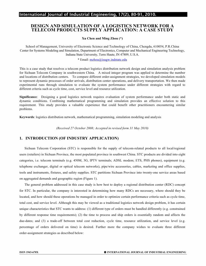
Table 3: Capacity and utilization of resources at DCs

Outputs SD PA1 PA2

DC1 4 / 0.811 2 / 0.05 2 / 0.502

DC2 25 / 0.827 2 / 0.248 6 / 0.852

DC3 80 / 0.91 180 / 0.91 160 / 0.906

DC4 5 / 0.569 2 / 0.034 2 / 0.334

DC5 12 / 0.736 2 / 0.104 3 / 0.698

DC6 40 / 0.857 2 / 0.379 15 / 0.607

DC7 26 / 0.824 2 / 0.224 7 / 0.779

Total units (# crews) 192 192 195

Avg. utilization (%) 79.1%* 27.8%* 66.8%*

* = significantly different from others at 95% confidence level. It is interesting to compare the results of the three strategies. The “best” solution really depends on the criterion used in

the evaluation. Given that we tried to maintain the average cycle time around eight days and queue length of waiting

orders less than ten at each RDC, it seems that strategy PA2 is the best (Table 2) in the sense that it resulted in the highest

overall service level. But PA1 would be the best if we only look at the total cost (it resulted in the least total cost).

However, if we look at resource utilization and operational cost at RDC, strategy SD is clearly the winner (Note that based

on the current data provided, transportation cost dominates the total cost). In simulation, the total cost included two parts:

operation cost and transportation cost. STC suggested using a cost coefficient per operational crew per unit of time for the

operation cost that includes labor, equipment and utilities. The experimental results were discussed with STC staff, and

were considered valid by STC managers. We also like to point out the fact that the data collected during was limited (e.g.

operation cost was estimated by STC based on current practice, order type was estimated using one year’s data, “order

processing time” at RDC was estimated based on STC Chen Du Branch operation, etc.), the models built at current stage

is still under the improvement. However the models have had a robust and flexible structure that allows more effective

functions to be added or built in to improve simulation performance and model fidelity. The suggestions made to STC

include collecting more data to better characterize orders (e.g. order arrival, type, and quantity distribution), processing

time at RDC, and transportation time. 5. CONCLUSIONS AND FUTURE STUDY This industry application addressed a logistics network design problem that takes into account different

order-assignment strategies. We first formulated a mixed integer program to determine the number and locations of

distribution centers, and then developed simulation models to compare three different order-assignment strategies in terms

of average cycle time, service level, total cost and resource utilization. Although the models developed are under further

improvement through better data modeling and characterization, the effort has significantly improved the performance of

STC logistics and distribution. According to reported feedback by STC, this study has helped the company make

important decisions that improved the performance of their logistics and distribution, decreased inventory and increased

Chen and Zhou

90

service level, and achieved significant cost savings. By implementing the results of the study, e.g. establishing the seven

RDCs and reassigning orders according the proposed strategies, plus other effort that STC made to improve its operational

efficiency, the company has reduced the capital tied up with inventory by 40%, resulted in a saving of RMB 73,754,357.

The average inventory turnover time has decreased to 22 days, which is comparable to the current inventory turnover time

of DELL Company. The overall service level has also been greatly improved to a level around 90%.

Also for the first time, the company adopted a quantitative approach to objectively and scientifically analyze its

logistics performance via simulation models. It also reduced the requirement of “experience” for (or reliance on)

managerial staff. The results provided a robust basis for carrying out the study planned for next step, in which STC is

interested in estimating a relationship between the total cost and specified service level. Let β* be the set of regression

coefficients corresponding to the best model configuration identified, X the service level, and Y the minimum total cost

corresponding to X. We would like to estimate a linear relationship through following regression: Y = β0 + β1X+ ε, where

ε is a random error term. However, service level X essentially depends on other factors that are more operable, such as

resource capacity X1 (e.g. number of handling crews at RDCs) and delivery time X2 (a total of picking/processing time and

transportation time). Therefore a more practical regression is: Y = β0 + β1X2 + β2 X2 + ε. We plan to make experimental

runs through the simulation models to collect data for estimating the set of regression coefficients. The regression built

through such simulation will be validated through the field data. Given the definition of the service level (i.e. percentage

of COs delivered on time), it is possible to identify the combinations of X1 and X2 mapped on a range of commonly

specified discrete scale [90%, 91%, 92%, 93%, 94%, 95%]. Then through the regression we can estimate the total cost

associated with these commonly specified service level. This will be valuable to help STC logistics managers in making

the trade-off decisions to balance total logistics cost and service level requirement or other factors. 6. REFERENCES 1. Banks, J. (editor) (1998). Handbook of Simulation, Principles, Methodology, Advances, Applications, and Practice.

John Wiley & Sons, Inc. New York.

2. Bowersox, D. J., D. J. Closs and M. B. Cooper. (2002). Supply Chain Logistics Management. McGraw Hill, Boston.

3. Cormen, T.H., C. E. Leiserson and R. L. Rivest. (1999). Introduction to Algorithms. The MIT Press, Massachusetts.

4. Ghiani, G., G. Laporte and R. Musmanno. (2004). Introduction to Logistics Systems Planning and Control. John

Wiley & Sons, New York.

5. Kelton W. D., R. P. Sadowski and D. T. Sturrock. (2007). Simulation with Arena. McGraw Hill, Boston.

6. Montgomery, D. C. (1991). Design and Analysis of Experiments. John Wiley & Sons, New York.

7. Ratliff, Donald H., William G. Nulty, (1996). Logistics Composite Modeling. The Logistics Institute at Georgia Tech,

Atlanta, Georgia.

8. Robinson, Stewart. (2004). Designing the Conceptual model in Simulation Studies. Proceedings of the 2004

Operational Research Society Simulation Workshop. Operational Research Society, Birmingham, UK, 259-266.

9. Zhou, M., Son, Y.J., & Chen, Z. (2004). Knowledge representation for conceptual simulation modeling.

Proceedings of the 2004 Winter Simulation Conference, ed., R.G. Ingalls, M.D. Rossetti, J.S. Smith, and B.A.

Peters. Institute of Electrical and Electronics Engineers, Piscataway, NJ.


91

BIOGRAPHICAL SKETCH

Xu Chen is a professor at the School of Management and Economics, University of

Electronic Science and Technology of China, also the Director of Management Science

and Engineering Research Center and the Head of Management Science & E-commerce

Department of the university. He received a Ph.D. in Management Science and

Engineering from Southwest Jiaotong University in 2000, and had been a visiting

scholar at UC Berkeley in 2009. Dr. Chen’s research interests include logistics

simulation, supply chain management, service operations management and revenue

management. His email address is [email protected].

MING ZHOU is a professor at Indiana State University, also the director and chief

researcher at the Center for Systems Modeling and Simulation of the university. He

received a Ph.D. in Systems and Industrial Engineering from the University of Arizona

in 1995. Dr. Zhou’s research interests include knowledge based simulation, intelligent

decision support systems for manufacturing, modeling and simulation of

logistics/distribution and supply chain systems. He has been a member of IIE and

serving on the editorial board for International Journal of Industrial Engineering (since

1997) and Journal of Simulation (since 2006). Dr. Zhou’s email address is

<[email protected]>.

Documents

DESIGN AND SIMULATION OF A LOGISTICS NETWORK FOR A TELECOM …