Design and Validation of a Low Cost, Partial Flow Dilution Tunnel with

Tapered Element Oscillating Microbalance

A Thesis

Presented in Partial Fulfillment of the Requirements for the

Degree of Master of Science

with a

Major in Mechanical Engineering

in the

College of Graduate Studies

University of Idaho

by

Victor Christensen

May 2010

Major Professor: Steven W. Beyerlein, Ph.D.

ii

Authorization to Submit Thesis

This thesis of Victor Christensen, submitted for the degree of Master of Science with

a major in Mechanical Engineering and titled " Design and Validation of a Low Cost, Partial

Flow Dilution Tunnel with Tapered Element Oscillating Microbalance”, has been reviewed

in final form. Permission, as indicated by the signatures and dates given below, is now

granted to submit final copies to the College of Graduate Studies for approval.

Major Professor _____________________________________Date______________

Steven W. Beyerlein, Ph.D.

Committee

Members _____________________________________Date______________

Judi Steciak, Ph.D.

_____________________________________Date_______________

Jon Van Gerpen, Ph.D.

Mechanical

Engineering Chair ____________________________________Date______________

John Crepeau, Ph.D.

College of

Engineering Dean _____________________________________Date_______________

Donald Blackketter, Ph.D.

Final Approval and Acceptance by the College of Graduate Studies

_____________________________________Date_______________

Margrit von Braun, Ph.D.

iii

Abstract

Accurate, repeatable measurement of tailpipe emissions is an important factor in the

development of internal combustion engines and testing of alternative fuels. A dilution tunnel

simulates the action of exhaust mixing with atmospheric gases and prevents condensation

prior to gas and particulate measurements. In this work, a micro dilution tunnel was designed

for the Small Engine Research Facility (SMERF) and experiments were conducted to

establish the controllability and accuracy of the tunnel. The tunnel design implements partial

flow, Constant Volume Sampling (CVS) using an ejector dilutor. In addition to a new 5 gas

Horiba MEXA 584L analyzer, a Tapered Element Oscillating Microbalance (TEOM) has

been deployed for real-time measurement of particulate emissions. Data from these

instruments and the flow conditioning equipment are collected and logged by a National

Instruments data acquisition system. For best results, the system should be operated at 700°

F suction temperature and 35 psia motive pressure to maintain a dilution ratio of 11:1 with

uncertainty of 3% at the 80% confidence level. A procedure has been developed for

obtaining and verifying dilution ratios between 11:1 and 15:1 with a 1.9L Volkswagen TDI

diesel. This new instrumentation will also be helpful in testing two-stroke snowmobile

engines that typically produce elevated levels of hydrocarbons and particulates beyond the

saturation range of many electro-chemical emissions analyzers.

iv

Acknowledgements

First and foremost, I would like to thank my major professor Dr. Steven Beyerlein for

his support and guidance throughout my time at the University of Idaho. Likewise, Dr. Judi

Steciak has been an indispensable resource both in and out of the classroom during my

research. Invaluable in day-to-day problem solving and brainstorming; I could not have

completed this work without the assistance of Dr. Dan Cordon. Lastly, I would like to thank

the National Institute for Advanced Transportation Technology (NIATT) and the Idaho

Higher Education Research Council (HERC) for their generous financial support of this

project.

v

Table of Contents

Authorization to Submit Thesis ............................................................................................. ii

Abstract ................................................................................................................................... iii

Acknowledgements ................................................................................................................ iv

Table of Contents .................................................................................................................... v

List of Figures ........................................................................................................................ vii

List of Tables ........................................................................................................................ viii

Chapter 1: Introduction ........................................................................................................ 1

Chapter 2: Emissions Testing and Dilution Tunnels .......................................................... 4

2.1 – Gaseous Emissions and Detection ............................................................................... 4

2.2 – Particulate Formation and Detection ........................................................................... 8 2.3 – Dilution Tunnel Sampling.......................................................................................... 13

Chapter 3: Dilution Tunnel Design .................................................................................... 18

3.1 - System Level Design .................................................................................................. 18

3.2 - Component Selection .................................................................................................. 20

3.3 - Dilution Ratio Control ................................................................................................ 25 3.4 - Data Acquisition Software .......................................................................................... 27

3.5 - Detail Design .............................................................................................................. 33

Chapter 4: Dilution Tunnel Validation ............................................................................... 41

4.1 - Dilution Device Calibration........................................................................................ 41

4.2 - Labview Calibration ................................................................................................... 46 4.3 - Bench Testing with Calibration Gas ........................................................................... 48 4.4 – Engine Testing ........................................................................................................... 51

Chapter 5: Conclusions and Recommendations ................................................................ 56

References .............................................................................................................................. 62

Appendix A: Dilution Tunnel Operating Procedures........................................................ 64

Appendix B: Labview Interface ........................................................................................... 71

Appendix C: Detail Drawings .............................................................................................. 79

vi

Appendix D: Resistor Bank Test Setup .............................................................................. 89

Appendix E: Component Specification Sheets ................................................................... 94

Fox Ejector Dilutor ............................................................................................................. 94 Thermo Scientific TEOM 1400ab ...................................................................................... 95 Horiba MEXA-584L ........................................................................................................... 96 Omega CN2110 – T10 ........................................................................................................ 97

vii

List of Figures

Figure 1: Operating principles of NDIR - CO2 & CO absorption spectrum [2] ....................... 6

Figure 2: Particulate composition by mass [4] ......................................................................... 9 Figure 3: Internal features of Tapered Element Oscillating Microbalance [8] ....................... 12 Figure 4: Dilution effects on diluted humidity and temperature [12] ..................................... 14 Figure 5: Deposition effects of sudden expansion [14] .......................................................... 17 Figure 6: System diagram of dilution tunnel design ............................................................... 19

Figure 7: Ejector dilutor operating principals [15] ................................................................. 20 Figure 8: Thermo Scientific TEOM model 1400ab [15] ........................................................ 21 Figure 9: Horiba MEXA 584L 5-gas analyzer ....................................................................... 23 Figure 10: Hewlett Packard VXI Data acquisition unit .......................................................... 25

Figure 11: Circuit diagram of Dilution ratio acquisition system ............................................ 28 Figure 12: Schematic design of Labview interface................................................................. 30 Figure 13: Main Labview interface for data acquisition using dilution tunnel....................... 31

Figure 14: Status and Logging interface ................................................................................. 32 Figure 15: Sample data file created by Labview interface ..................................................... 33

Figure 16: Line heater design with temperature and pressure sensor. .................................... 35 Figure 17: Tunnel body with transducer and sampling lines .................................................. 36 Figure 18: Side profile of sample line fittings. ....................................................................... 36

Figure 19: Control schematic for ejector dilutor ..................................................................... 37 Figure 20: Omega CN2110-T10 PID temperature controller with 10 amp solid state relay .. 38

Figure 21: Detail design for dilution tunnel cart ..................................................................... 39 Figure 22: Dilution tunnel system cart .................................................................................... 40 Figure 23: Dilution ratios at three different set points as calculated by two different methods

......................................................................................................................................... 42

Figure 24: Dilution ratio as a function of suction temperature with constant motive pressure

measured with CO2 cal-gas dilution ............................................................................... 43 Figure 25: Dilution ratio as a function of motive pressure with constant temperature data sets

measured using CO2 cal-gas dilution .............................................................................. 44 Figure 26: Sub-VI for calibration of the dilution tunnel sensors with gain and bias constants

highlighted. ..................................................................................................................... 47

Figure 27: Engine testing test setup ........................................................................................ 52

Figure 28: Exhaust gas CO2 measurement at 700° F, 35 psia with 80% confidence interval . 55

Figure 29: NIATT dilution tunnel front view ......................................................................... 57

Figure 30: NIATT dilution tunnel right side view .................................................................. 58 Figure 31: NIATT dilution tunnel left side view .................................................................... 59

viii

List of Tables

Table 1: Table of analog channels on data acquisition ........................................................... 29 Table 2: Measured set points for known dilution ratios ......................................................... 45 Table 3: Constituents of calibration gases used for validation ............................................... 49 Table 4: Results from testing cal-gas 1 ................................................................................... 49 Table 5: Results from testing cal-gas 2 ................................................................................... 50

Table 6: Results from testing cal-gas 3 ................................................................................... 50 Table 7: Results from testing cal-gas 4 ................................................................................... 50

Table 8: Dilution ratio correlation between engine exhaust and CO2 at 700° F suction

temperature ..................................................................................................................... 53

Table 9: Results of engine exhaust dilution measurements .................................................... 53

Table 10: Recommended set points for future tunnel operation, and associated error in

dilution ratio .................................................................................................................... 54 Table 11: NIATT dilution tunnel specifications ..................................................................... 56

1

Chapter 1: Introduction

Emissions from internal combustion engines are a significant concern both as

potential health hazards, and as contributors to environmental issues, such as

photochemical smog and climate change. Of particular interest are nitrogen oxides,

carbon dioxide, carbon monoxide, hydrocarbons, and particulate matter. These

pollutants can be detected by numerous methods, using either raw exhaust treated to

remove water or diluting the exhaust with air to lower the dew point of the mixture.

Dilution tunnels have been shown by Kittleson, et al., to mimic mixing of exhaust

pollutants that occurs as the exhaust exits the tailpipe of a vehicle [1]. Additionally, the

dilution process “freezes” the exhaust – preventing chemical decomposition of exhaust

constituents. Most commercial solutions dilute the full exhaust flow, at a minimum of

4:1 dilution ratio. Full flow systems, however, can be very large and prohibitively

expensive. Micro dilution tunnels only sample a small portion of the exhaust, which

although less accurate, is significantly cheaper and smaller.

Development of a micro dilution tunnel at the University of Idaho was

undertaken to expand research capabilities in engine research and emission analysis.

Due to the large variety of internal combustion (IC) engine testing taking place at the

University of Idaho, a dilution tunnel was chosen as the best instrument to be used in

testing. Using a dilution tunnel, one can test anything from a diesel engine that

generates high levels of particulate matter and NOx, to a two-stroke engine that may

release elevated levels of hydrocarbons that would saturate an ordinary gas analyzer.

Additionally, the dilution tunnel does an excellent job of freezing the exhaust

2

composition, preventing possible line contamination or continuing reactions in the hot

exhaust gas. Design of the dilution tunnel was centered on meeting these research

needs and goals.

In Chapter 2, preliminary research into emission formation is introduced to

better understand both the behavior of engine emissions, and the best practices of

detecting emissions in a laboratory setting, including which sensors would work best

for the application. This particularly applied to the case of engine soot or particulate

matter detection, since this is an area in which technology is still developing.

Additionally, the field of dilution tunnels was explored to determine best practices for

design and construction of a micro-dilution tunnel. From this research, a preliminary

dilution tunnel system was designed utilizing the most appropriate component choices

for the application.

Guided by information obtained from this research, Chapter 3 details several

design decisions that were made as to major components of the dilution tunnel. These

components were critical to producing the functionality needed for IC engine research,

and were central to the overall design of the dilution tunnel. Once the critical functional

components were obtained, testing was done to determine methods for control of the

functioning parts of the dilution tunnel, and means to log data via electronic data

acquisition (EDAC). As a final step, the detailed design of the tunnel was completed with

all functional components, and fabrication took place to construct the final testing

platform. Upon completion of fabrication, all that remained to complete was calibration

of the control systems and validation of the tunnel apparatus as a whole.

3

Chapter 4 presents the final design of the dilution tunnel. As constructed, the

systems that controlled the dilution process needed to be calibrated to allow both

control of the dilution, and accurate and repeatable measurements of the rate of

dilution in the tunnel apparatus. This process was attempted with several methods,

eventually resulting in a calibration process that both worked, and provided accurate

and repeatable results. Once the calibration of the tunnel was completed, tests were

performed on various gases to validate that the control scheme was, in fact, working as

it should. These tests also served to help establish the limits of accuracy that the

dilution tunnel is able to deliver. As final validation and testing, the dilution tunnel was

used to sample engine exhaust from a Volkswagen TDI diesel engine. This data helped

establish experimental error for the dilution tunnel and provided lessons that would

help in future testing. Discussion of results and recommendations for tunnel operation

are reported in Chapter 5, including confidence intervals on measured dilution ratios.

4

Chapter 2: Emissions Testing and Dilution Tunnels

In the design of any system, it is first necessary to understand both the behavior

of the system, and the desired functional requirements of the design. Before attempting

the design of an emission sensing apparatus, it was first necessary to understand the

nature of emissions in general, and the principles involved in detecting emissions. The

preliminary research presented in this section, was conducted into the two main types

of emissions that IC engines produce. First, gaseous emissions such as CO, CO2, and NO,

were explored to understand general formation and methods of detection, rather than

to develop a complete understanding of the chemical kinetics and equilibrium

mechanism. Secondly, the formation and detection of engine soot or particulate matter

was researched with emphasis on feasible methods of detection. Finally, the field of

dilution tunnels was explored to determine best practices for design and construction

of a micro-dilution tunnel. This research was used to guide design decisions, and assist

in component selection for critical systems.

2.1 – Gaseous Emissions and Detection

Gaseous emissions of concern from internal combustion engines primarily

include CO, CO2, NO, and unburned hydrocarbons. Each of these emissions has its own

environmental and human hazards, and method of detection.

The primary pollutant from any internal combustion engine burning a

hydrocarbon fuel is carbon dioxide. This is because CO2 is a necessary product of the

combustion process. By itself, CO2 is not an inherently dangerous emission. It is non-

5

toxic, except in very large concentrations, and causes no short-term environmental

effects. However, CO2 has been identified as a greenhouse gas, carrying with it global

warming potential. Most notably, it has been announced recently that the United States

is officially recognizing greenhouse gases as dangerous substances, promising to be the

precursor to future legislation by the Environmental Protection Agency. For the

purposes of most engine research however, CO2 is a “least of all evils” emission; the

more efficient the combustion, the more CO2 created and the less unburned

hydrocarbons and CO that will be released into the atmosphere. For this reason,

emission measurement of CO2 is primarily used as a measure of complete combustion

[2], or for the purpose of determining total carbon output.

The majority of harmful emissions from internal combustion engines are in the

form of NO, CO and unburned hydrocarbons, although there are small concentrations of

SO2 (from sulfur-containing fuel and lubricants) and other pollutants. These three

pollutants are responsible for the majority of health and environmental harm that can

be traced to internal combustion engine use. Detection of gaseous emissions is

accomplished in a number of ways, using a number of sensor technologies. The simplest

sensor technology is an electro-chemical sensor. This type of sensor contains

electrolytic compounds (usually acids) that are reactive to a certain species of gas.

When the sensor is exposed to the gas, reactions will occur proportionally to the

concentration of the gas – causing an electrical potential difference in the sensor cell

[2]. These sensors have the advantage of being inexpensive, and fairly accurate, but are

consumable, subject to long-term sensor drift, and ultimately do not have the accuracy

of a more expensive sensor.

6

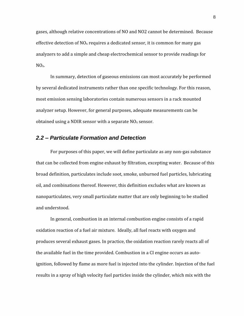
Another common method of measurement is using infrared (IR) spectroscopy.

This method takes advantage of the IR absorbing properties of gases by passing a beam

of IR light through the gases, and measuring the amount of IR absorbed by the gases in

certain areas of the IR spectrum. Figure 1 shows the absorption spectrum of CO2.

Figure 1: Operating principles of NDIR - CO2 & CO absorption spectrum [2]

The infrared spectroscopy sensing technology most commonly used is the Non-

Dispersive InfraRed sensor (NDIR). As previously described, NDIR sensors measure the

spectrum and amplitude of infrared absorption and correlate it to relative amounts of

species. NDIR can be calibrated to the absorption spectrums of CO2, CO, and numerous

hydrocarbons, and used to identify the relative quantities present in the sample.

7

However, for the NDIR sensor to work properly, one must be aware of and avoid

crossover absorptions. The NDIR sensor measures only the amount of energy absorbed

and, from its calibration, infers a concentration of gas. However, in the specific case of

CO2, water vapor also absorbs IR on some of the same wavelengths as CO2, which can

lead to significant error in the reading of CO2 [2]. This means that unless water can be

eliminated from the sample gas, the CO2 measurement will be significantly inaccurate.

Removal of water vapor from exhaust is most commonly accomplished by passing the

exhaust gases through an ice bath to condense the water vapor. This sufficiently dries

the sample to ensure that measurement of CO2 will be accurate.

In some engine applications, emissions such as hydrocarbons and NO are in low

enough concentrations that IR detection is not accurate enough. This means that

additional sensing technologies are often needed to complete measurement of EPA

regulated emissions. For unburned hydrocarbons, a very common sensor is Flame

Ionization Detection (FID), which measures flame ionization changes when the sample

is injected into fuel. This technology is more accurate than NDIR, but has the down side

that the unburned hydrocarbon species (e.g. hexane, methane, etc.) cannot be

determined – only the amount [2].

Nitrogen oxides (NO, NO2, or NOx for short) are the primary cause of

photochemical smog. Detection of NOx is most commonly done using a

chemiluminescent NOx sensor. Chemiluminescence is a process by which NO reacts

with O3 (ozone) and emits a photon after reaction. Exhaust is pretreated using catalysts

or reducing agents to convert all NO2 to NO before reaction. By measuring the amount

of light emitted from the sample gas, NOx concentration can be inferred in the sample

8

gases, although relative concentrations of NO and NO2 cannot be determined. Because

effective detection of NOx requires a dedicated sensor, it is common for many gas

analyzers to add a simple and cheap electrochemical sensor to provide readings for

NOx.

In summary, detection of gaseous emissions can most accurately be performed

by several dedicated instruments rather than one specific technology. For this reason,

most emission sensing laboratories contain numerous sensors in a rack mounted

analyzer setup. However, for general purposes, adequate measurements can be

obtained using a NDIR sensor with a separate NOx sensor.

2.2 – Particulate Formation and Detection

For purposes of this paper, we will define particulate as any non-gas substance

that can be collected from engine exhaust by filtration, excepting water. Because of this

broad definition, particulates include soot, smoke, unburned fuel particles, lubricating

oil, and combinations thereof. However, this definition excludes what are known as

nanoparticulates, very small particulate matter that are only beginning to be studied

and understood.

In general, combustion in an internal combustion engine consists of a rapid

oxidation reaction of a fuel air mixture. Ideally, all fuel reacts with oxygen and

produces several exhaust gases. In practice, the oxidation reaction rarely reacts all of

the available fuel in the time provided. Combustion in a CI engine occurs as auto-

ignition, followed by flame as more fuel is injected into the cylinder. Injection of the fuel

results in a spray of high velocity fuel particles inside the cylinder, which mix with the

9

air and combust. Particulates form primarily where large particles of fuel react with air,

most often occurring near the nozzle of the injector, where there is an area of richer

fuel-air ratio. Because there is not enough oxygen present locally to fully react the fuel,

the fuel oxidizes partially, leaving a loose formation of carbon, and other unoxidized

substances [2].

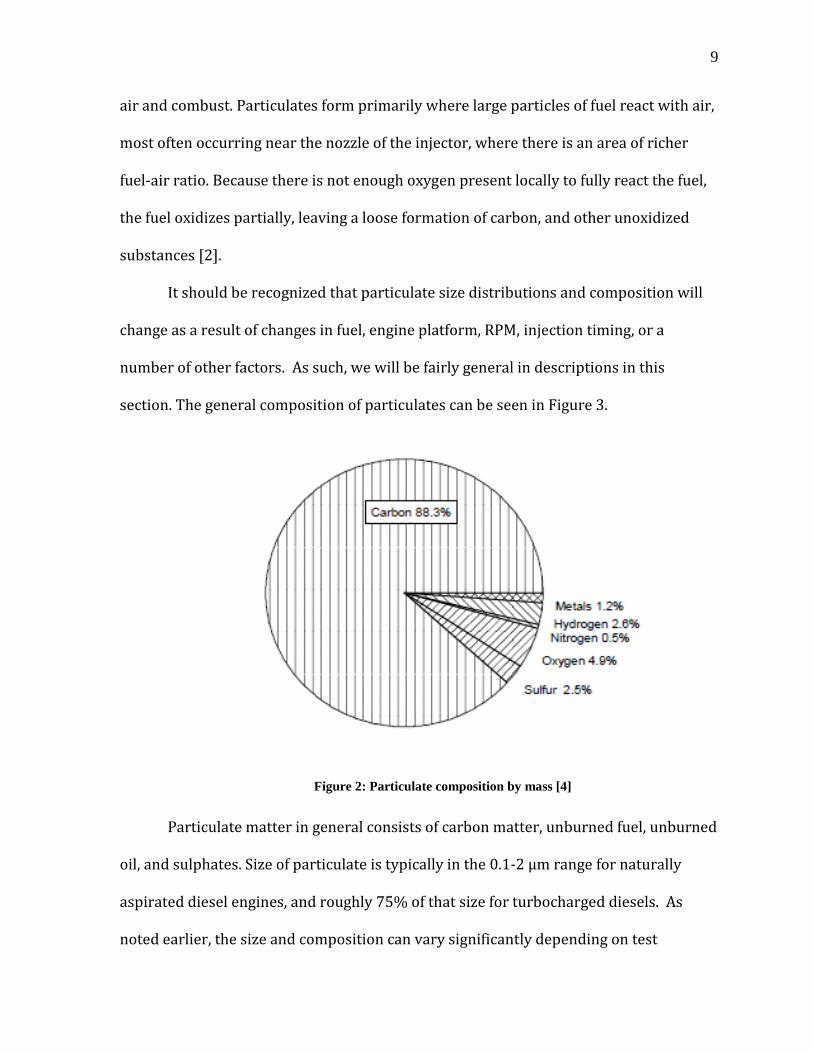
It should be recognized that particulate size distributions and composition will

change as a result of changes in fuel, engine platform, RPM, injection timing, or a

number of other factors. As such, we will be fairly general in descriptions in this

section. The general composition of particulates can be seen in Figure 3.

Figure 2: Particulate composition by mass [4]

Particulate matter in general consists of carbon matter, unburned fuel, unburned

oil, and sulphates. Size of particulate is typically in the 0.1-2 µm range for naturally

aspirated diesel engines, and roughly 75% of that size for turbocharged diesels. As

noted earlier, the size and composition can vary significantly depending on test

10

platform, but in general, the biggest contributors to particulate formation appear to be

fuel composition (specifically sulfur in fuel), engine lubricant [3], and engine design. As

will be discussed further in the next section, the differences between turbocharged and

naturally aspirated diesel engines can result in significantly less particulate matter for

the turbocharged design.

By far, the most common (and EPA certified) method of detecting and measuring

exhaust particulate is the gravimetric method. Simply put, gravimetric analysis consists

of directing exhaust samples through one or more filters, and weighing the filters on a

precision balance both before and after the test. The difference in mass before and after

is the mass of particulate collected. This method has the advantage of being very

accurate and repeatable, as transient changes are averaged out over the course of the

test. However, this method is unable to provide any data on size or mass distribution,

nor can it provide any data on transient emissions [6].

Gravimetric testing is most often used with Constant Volume Sampling (CVS)

which considerably simplifies recording the volume of exhaust passed through the

filter. CVS dilutes the exhaust with air at a set dilution ratio – providing a constant flow

rate throughout the test. Once the test is complete, the filter is weighed and the

particulate rate is calculated by the following equation:

𝑃𝑎𝑟𝑡𝑖𝑐𝑢𝑙𝑎𝑡𝑒 𝑅𝑎𝑡𝑒 =𝑀𝑎𝑠𝑠 𝑃𝑎𝑟𝑡𝑖𝑐𝑢𝑙𝑎𝑡𝑒

𝑉𝑜𝑙𝑢𝑚𝑒𝑡𝑟𝑖𝑐 𝑓𝑙𝑜𝑤 ∗ 𝑇𝑖𝑚𝑒

A major advantage to gravimetric testing is that it is stable and repeatable, and

unaffected by water. After the test, the filters are allowed to equilibrate at controlled

humidity, removing extraneous water, preventing erroneous data. The big disadvantage

11

of gravimetric detection is the slow testing rate, and sensitivity of testing [6]. Unless the

system is automated, it is very possible for filters to be contaminated, throwing

measurements off. Additionally, gravimetric testing can be very expensive and

resource intensive due to the need for new filters each test.

Another method of measuring particulate is Laser Induced Incandescence (LII).

This method uses a scanning laser to heat particulate matter in a gas stream to a

temperature where the particle will emit incandescent light briefly as it cools. By

measuring the duration of emitted light and making some assumptions about particle

composition, this sensor can measure volume fraction of particulate in the exhaust flow.

This measurement involves considerable amount of post-processing of data to produce

measurements making LII somewhat impractical for general testing uses. Additionally,

this technique relies on several assumptions about the density and constituency of

particulate, meaning that mass measurements can be affected by changes in fuels, or

engine platform. For these reasons, LII will probably continue to be more of a research

tool than an EPA certification tool that can be easily used in a testing environment.

The final particulate measurement technology presented here is the Tapered

Element Oscillating Microbalance or TEOM. A TEOM consists of a tapered, cantilever

element forced to oscillate by an electronic feedback system. On the end of the

cantilever element is a filter, through which the sample passes at a fixed volumetric

flow rate. As the filter accumulates particulate mass, the frequency of the element

oscillation changes, which gets picked up by the feedback system. This instrument can

detect particulate concentration in a short sample time (as small as 0.21 sec [7]), giving

12

immediate readings of particulate mass. Figure 3 shows the basic features and

operation of the TEOM.

Figure 3: Internal features of Tapered Element Oscillating Microbalance [8]

Numerous studies [7;9;10;11] have been performed to determine the TEOM’s

ability to provide as accurate results as gravimetric particulate testing. In general, due

to filter efficiencies, TEOMs seem to always read particle concentrations lower than

equivalent gravimetric tests, mostly due to filter inefficiency collecting smaller

particulates. As the technology has matured, the accuracy has improved from 9-14% [9]

underreporting to about 6% [10] underreporting when compared with gravimetric

results. This improvement can be linked primarily to improvements in filter efficiency

due to improved filter media [10]. Additionally, original reports of inaccuracies in

TEOM measurements can be at least partially attributed to vibration or moisture [11].

13

Some major drawbacks of TEOM measurements are loss of particulate matter,

sensitivity to moisture, sensitivity to vibration, and susceptibility to saturation. The size

and material of the filter leads to lower efficiency for smaller particulates when

compared to gravimetric filter technology. Since a portion of the particulate can pass

through the TEOM filters, this contributes to lower sensor resolution and

underreporting by the instrument. Additionally, because the filter is not hydrophobic,

particulate measurements can be affected by water vapor unless the sample is treated

to reduce water, often resulting in particulate loss. Sensitivity to vibration can also

cause large discrepancies in readings due to interference with the vibration of the

tapered element. Lastly, if used on raw exhaust, the small face area of the filter

(approximately 15mm in diameter) can become fouled in a short period of time,

requiring frequent replacement. However, if the TEOM can be isolated from vibration

and used to sample diluted exhaust, rather than raw exhaust, a TEOM can be an

affordable and accurate substitute for gravimetric testing.

2.3 – Dilution Tunnel Sampling

The purpose of a dilution tunnel is to dilute raw engine exhaust with a cool gas,

both to freeze composition, and lower dew point of the incoming gases. A dilution

tunnel mixes the engine exhaust flow with a dilutant gas in a known ratio, called a

dilution ratio as shown below.

𝐷𝑖𝑙𝑢𝑡𝑖𝑜𝑛 𝑟𝑎𝑡𝑖𝑜 =𝑉𝑜𝑙𝑢𝑚𝑒𝑑𝑖𝑙𝑢𝑡𝑎𝑛𝑡

𝑉𝑜𝑙𝑢𝑚𝑒𝑒𝑥ℎ𝑎𝑢𝑠𝑡

14

As the engine exhaust is mixed with the dilutant stream, the exhaust is cooled

rapidly. This has the effect of stopping reactions that are still occurring in the exhaust,

“freezing” the chemical composition. Additionally, because the dilutant stream contains

very little water, the dilution process lowers the dew point in the mixture to much

lower levels than in raw exhaust. Lowering the dew point eliminates the need for

heated lines or desiccant drying procedures to prevent water condensation inside

sensors or handling apparatus. This results in improved cost, reliability, and reduction

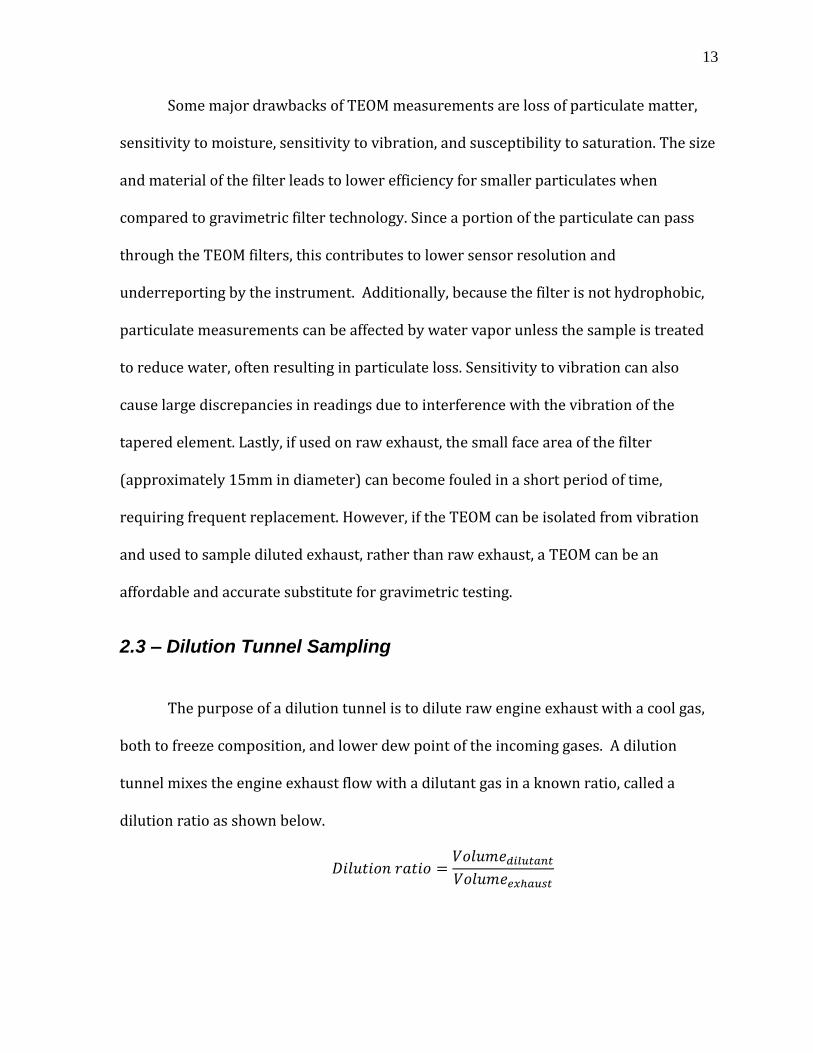
of potential sensor problems in downstream gas sensors. Figure 4 shows the effect of

dilution ratio on downstream temperature and relative humidity when sampling

exhaust at 900° F (Approx 500° C). We can see that at a dilution ratio of 10:1 and above,

the resultant humidity will not cause condensation in sample lines or sensors.

Figure 4: Dilution effects on diluted humidity and temperature [12]

15

Once the exhaust gas has been diluted, it can be sampled by an emission analyzer

for quantities of pollutant. These quantities are then multiplied by the dilution ratio,

resulting in raw concentrations of the measured emission. For example if a flow is

diluted 10:1 and the diluted stream contains 50 ppm of NO, the exhaust stream must

contain 50 ppm x 10 = 500 ppm of NO.

Dilution tunnels come broadly under two categories – full flow dilution tunnels,

and partial flow tunnels. As the name implies, a full flow dilution tunnel samples the

entire exhaust flow from an internal combustion engine and mixes it with a dilution

gas[13]. Because of the volumes of exhaust, the dilutant is most commonly ambient air,

and even with high flow components, the dilution ratios on a full flow tunnel will rarely

reach as high as 10:1. Partial flow tunnels will take some portion of an internal

combustion engine exhaust and dilute it with dilutant in the same way as a full flow

tunnel, but in much smaller proportions.

Full flow dilution tunnels are most commonly used in emission testing facilities,

where emissions are measured in total amounts as mandated by Federal Test

Procedures (FTP). An internal combustion engine will be attached to a dynamometer

and operated at specified RPMs and loads for given times, while emissions are collected

and recorded. Because no exhaust is allowed to escape, the repeatability of

measurements is generally agreed to be better than that obtained with a partial flow

tunnel [13]. Additionally, because of the low dilution ratios, less sensitive equipment is

necessary to measure emissions within the required accuracy. This is important in very

sensitive measurements, such as those required to certify a vehicles emission level. The

full flow tunnels require a large amount of air handling equipment in order to supply

16

the volume of air needed to dilute the entire flow of exhaust. Typically, for these lower

dilution ratios, there are often issues with water fouling, as the dewpoint is still high

enough to cause condensation in sample lines.

Partial flow tunnels are commonly used in smaller laboratory setups. Partial

flow tunnels have many benefits over full flow tunnels, including size, cost, and

maintenance. Partial flow systems can be considerably smaller than a full flow system,

allowing them to be used in small lab or portable setups. By their nature, they sample

only a portion of the exhaust gases, improving sensor response time by eliminating

fluctuations in dilution ratio or flow rates. Because of the smaller volumetric rates, it is

possible to achieve much higher dilution ratios in the partial flow tunnels; some tunnels

can get as high as 10,000:1 ratios [1], although these ratios are typically detrimental to

accurate readings, as the concentration of pollutants is orders of magnitude smaller

than raw exhaust, and requires very sensitive instruments to detect.

One regrettable truth about partial flow tunnels is that there are always

discrepancies in particulate matter when compared to full flow system. Much work has

gone to understanding and quantifying these losses, however there are many factors to

the losses. Several of the more significant reasons are transfer line effects, dilution ratio,

air pump used, and residence times. Transfer line effects stem from two sources: a) wall

cooling resulting in thermo-phoretic forces causing particulate deposition along the

walls of the transfer line, and b) sudden expansions [14]. This can not only lower

particulate readings, but can cause contamination of the testing if the deposits

randomly re-enter the exhaust stream. Figure 5 illustrates the process of deposition by

sudden expansion.

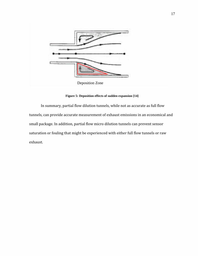
17

Figure 5: Deposition effects of sudden expansion [14]

In summary, partial flow dilution tunnels, while not as accurate as full flow

tunnels, can provide accurate measurement of exhaust emissions in an economical and

small package. In addition, partial flow micro dilution tunnels can prevent sensor

saturation or fouling that might be experienced with either full flow tunnels or raw

exhaust.

Deposition Zone

18

Chapter 3: Dilution Tunnel Design

3.1 - System Level Design

The design of the NIATT dilution tunnel was originally undertaken by a team of

mechanical engineering seniors as part of their senior capstone design class. The team

undertook preliminary analysis and research into dilution tunnel systems, and

purchased the dilution device to be used in further work. Following from the work done

by the senior design team, the overall design of the NIATT dilution tunnel was finalized

according to both their recommendations and the analysis of existing dilution tunnel

systems in Chapter 2 of this work.

The system level design for the dilution tunnel was chosen based on several

objectives: a) economy, both of size and cost, b) overall functionality, and c) ease of use.

It was decided to build a micro-dilution tunnel to keep the physical envelope small, a

large factor in the already crowded engine research facility. As a dilution device, an

ejector dilutor was determined to be the ideal component both due to the small physical

size and the lack of moving parts. The simplicity of the ejector dilutor operation

ensured both robust operation and ease of use on the overall system. Lastly, it was

decided to purchase a TEOM and portable gas analyzer as a cost effective means of

providing the most functionality for sensing both gaseous and particulate emissions.

These major components would be tied together using a data acquisition system

running National Instruments Labview software. This final piece was chosen for its

ability to combine outputs from the other components into one easy to use interface

19

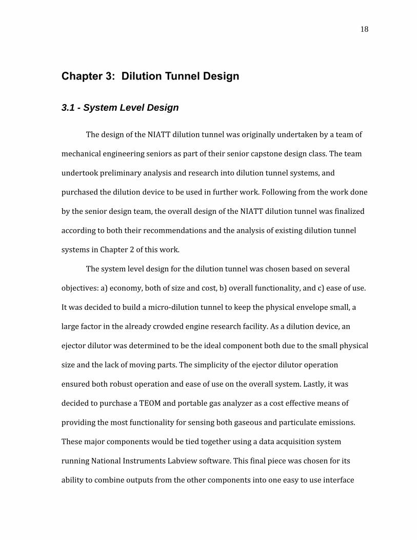
that also provides data logging in electronic form. This system level design can be seen

in Figure 6.

Figure 6: System diagram of dilution tunnel design

As shown in Figure 6, the NIATT micro dilution tunnel design dilutes a constant

volume of exhaust with dilution gas. This lowers the dew point of the mixture, and enables

instruments to test the mixture for pollutants without pretreatment that could modify the

composition. A dilutant, which most commonly would be compressed air, is introduced as

the motive flow in an ejector dilutor – drawing in engine exhaust from the suction line, and

mixing it into the dilution stream; functioning as the only pumping input for the micro

dilution tunnel. From the ejector dilutor, the diluted stream enters a sampling chamber, from

which sample flows are drawn into various sensors.

Sample streams enter a gas analyzer, determining concentration of hydrocarbons,

CO2, and other pollutants. A TEOM also is connected to the tunnel, which can determine the

concentration of particulate matter in the exhaust stream. Each of these components supplies

20

a signal to a data acquisition system that both displays the measurements and logs the data

electronically. Once through the sampling chamber, the remaining dilution stream is directed

out of the tunnel and into an exhaust collection system.

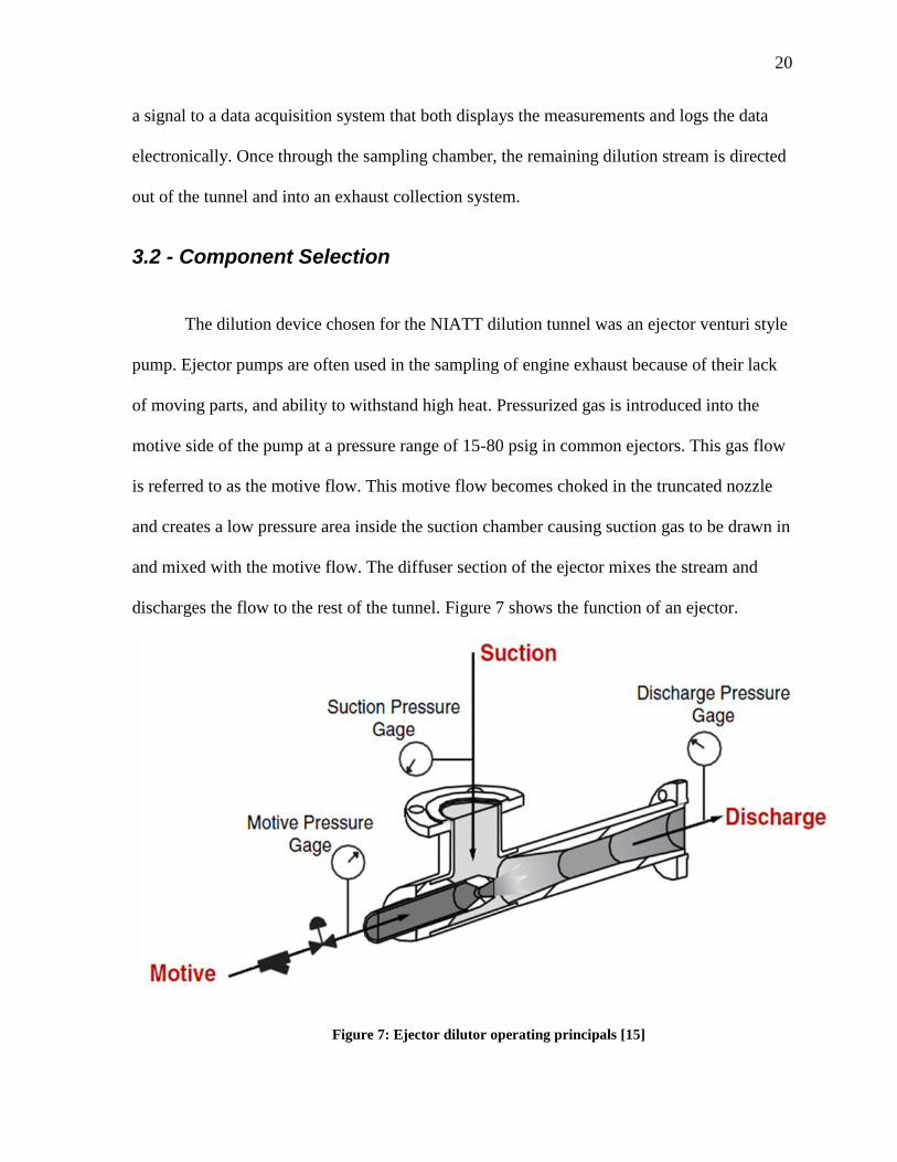
3.2 - Component Selection

The dilution device chosen for the NIATT dilution tunnel was an ejector venturi style

pump. Ejector pumps are often used in the sampling of engine exhaust because of their lack

of moving parts, and ability to withstand high heat. Pressurized gas is introduced into the

motive side of the pump at a pressure range of 15-80 psig in common ejectors. This gas flow

is referred to as the motive flow. This motive flow becomes choked in the truncated nozzle

and creates a low pressure area inside the suction chamber causing suction gas to be drawn in

and mixed with the motive flow. The diffuser section of the ejector mixes the stream and

discharges the flow to the rest of the tunnel. Figure 7 shows the function of an ejector.

Figure 7: Ejector dilutor operating principals [15]

21

The ejector acquired for the NIATT dilution tunnel was purchased from Fox Valves, a

manufacturer of custom critical flow venturi products. This ejector has a custom sonic choke

designed for a set dilution ratio of 10:1 at a suction temperature of 1000° F, although later

testing revealed that the actual dilution ratio was higher than advertised.

A critical functionality for the NIATT dilution tunnel was the ability to measure

particulate matter. A TEOM model 1400ab was purchased from Thermo Scientific to deliver

this functionality. This instrument was the primary model of TEOM manufactured by

Thermo Scientific at time of purchase, and was recommended for use by engineers working

for Thermo. Additionally, this model had been used in previous engine particulate studies

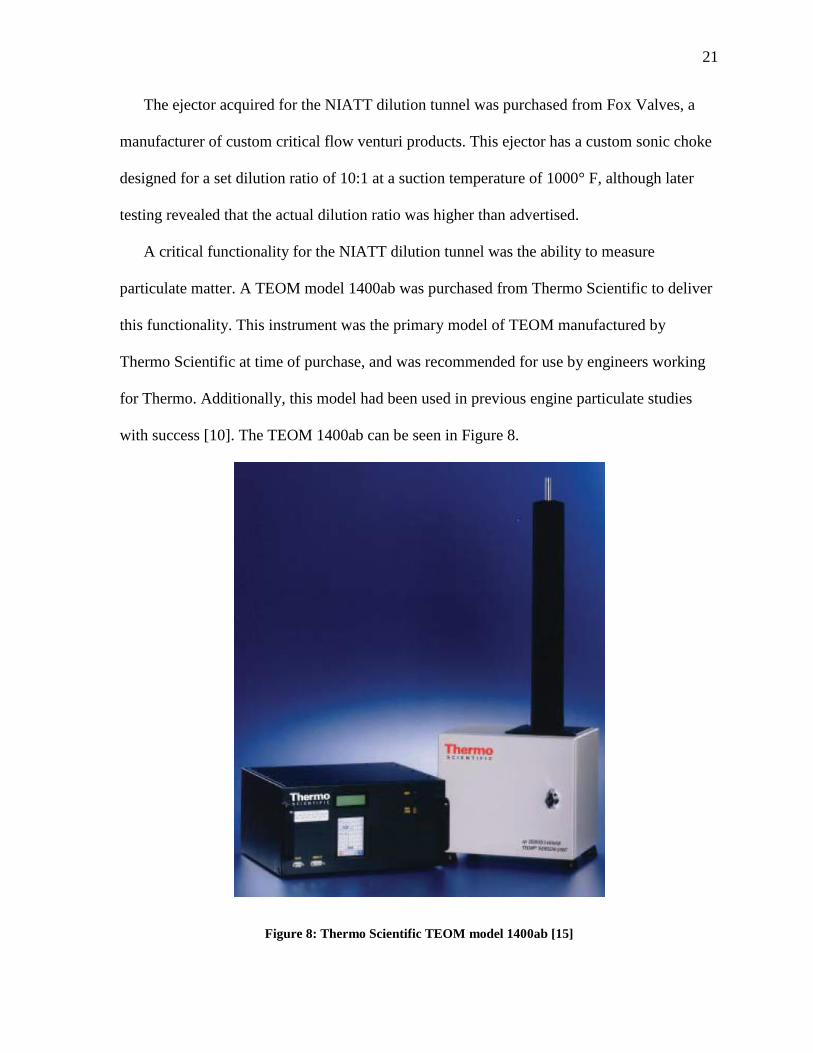
with success [10]. The TEOM 1400ab can be seen in Figure 8.

Figure 8: Thermo Scientific TEOM model 1400ab [15]

22

Due to dilution of the exhaust gases, gas analyzers used on dilution tunnels must have

higher resolution for pollutants than an analyzer used to test tailpipe emissions. The NIATT

tunnel is nominally designed to dilute exhaust in a 10:1 volumetric ratio, which means that

the relative concentrations for most pollutants will be 10 times smaller when sampled from

the dilution tunnel than when sampled from the tailpipe of an engine. For this reason, in a

dilution tunnel usage it is important to use an analyzer that has high resolution and precision,

to keep from losing overall accuracy in the instrument. Three major elements were identified

as being important features beyond the required precision of the analyzer: portability and

physical footprint, ability to produce analog output for data acquisition, and capacity to sense

all major species of pollutant (NOx, O2, CO2, CO, and HCs).

Several quotations were obtained from different manufacturers of emission sensing

equipment, and each was evaluated according to price and functionality as defined above.

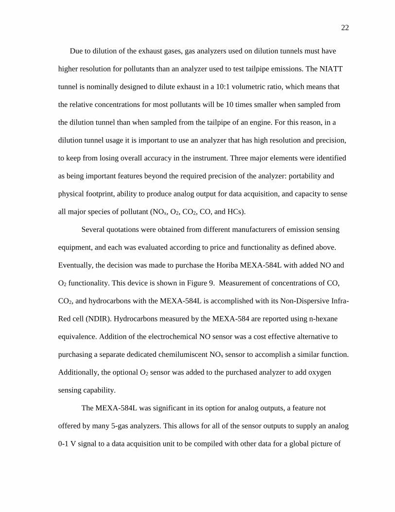
Eventually, the decision was made to purchase the Horiba MEXA-584L with added NO and

O2 functionality. This device is shown in Figure 9. Measurement of concentrations of CO,

CO2, and hydrocarbons with the MEXA-584L is accomplished with its Non-Dispersive Infra-

Red cell (NDIR). Hydrocarbons measured by the MEXA-584 are reported using n-hexane

equivalence. Addition of the electrochemical NO sensor was a cost effective alternative to

purchasing a separate dedicated chemilumiscent NOx sensor to accomplish a similar function.

Additionally, the optional O2 sensor was added to the purchased analyzer to add oxygen

sensing capability.

The MEXA-584L was significant in its option for analog outputs, a feature not

offered by many 5-gas analyzers. This allows for all of the sensor outputs to supply an analog

0-1 V signal to a data acquisition unit to be compiled with other data for a global picture of

23

the exhaust gas. Analog signal outputs, in combination with its small size and budget pricing

were the deciding factors for eventually purchasing this sensor from Horiba in August 2009.

In addition to sensing pollutants, this analyzer calculates the lambda parameter, and is

capable of sensing engine speed (RPM) using an induction sensor. When integrated into the

complete tunnel system, this analyzer provides output for acquisition and logging of

pollutants, correlated to engine RPM. The Lambda(λ) parameter is the ratio of actual air-to-

fuel ratio to stoichiometric , and can be expressed on a molar or, as below, mass basis.

λ =

(massair

massfuel)

actual

(massair

massfuel)

stoichiometric

This parameter is used to determine whether the engine is running in a fuel lean

condition (λ >1) or fuel rich condition (λ<1). The MEXA 584L can be used to calculate

Lambda according to the formula below. Because of the O2 present in dilutant air, this

Figure 9: Horiba MEXA 584L 5-gas analyzer

24

calculation would necessitate the sensor being either removed from the dilution tunnel or the

use of dry nitrogen as dilutant.

𝜆 =

[𝐶𝑂2] +[𝐶𝑂]

2 + [𝑂2] + {(𝐻𝑐𝑣

4 ∗3.5

3.5 +[𝐶𝑂]

[𝐶𝑂2]

−𝑂𝑐𝑣

2 ) ∗ ([𝐶𝑂2] + [𝐶𝑂])}

(1 +𝐻𝑐𝑣

4 −𝑂𝑐𝑣

2 ) ∗ {([𝐶𝑂2] + [𝐶𝑂]) + (𝐾1 ∗ [𝐻𝐶])}

Where:

[ ] is the concentration in % by volume, for HC only in ppm vol;

K1 is the conversion factor for HC expressed in ppmvol n-hexane (here 6 x 10^4)

Hcv is the atomic ratio of hydrogen to carbon in the fuel

Ocv is the atomic ratio of oxygen to carbon in the fuel

To collect and log measurements by the various components of the dilution tunnel, an

electronic data acquisition system was required. The primary data acquisition for the dilution

tunnel was chosen to be a Hewlett Packard VXI data acquisition unit shown in Figure 10.

This unit is rather large, which resulted in a larger space footprint than previously planned.

However, the VXI provides 30 channels of analog voltage input; bandwidth that allows all of

the acquisition necessary for the NIATT dilution tunnel. To accomplish data acquisition and

logging, each sensor input was connected to one of two multiplexer cards connected to the

VXI that provide multiple terminals for sensing voltage. These terminals can be measured by

the VXI’s voltmeter, and scaled to provide a real time reading. The VXI unit is connected

with a computer for acquisition and logging using National Instruments Labview software.

25

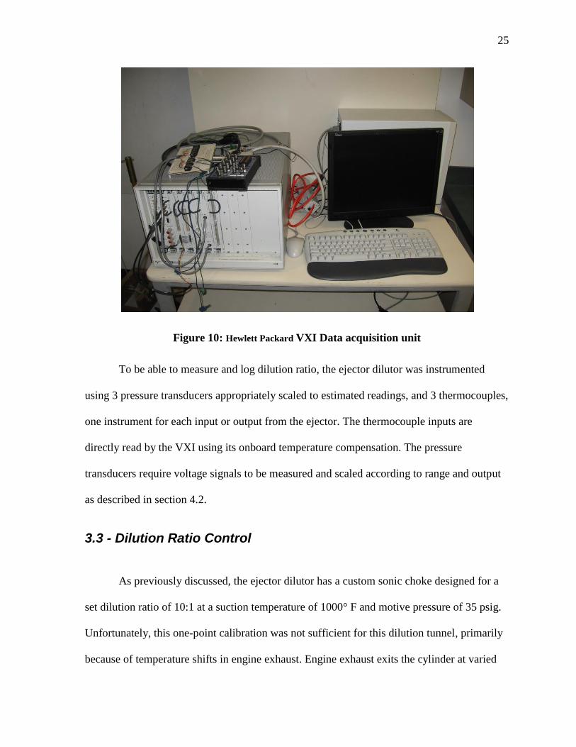
Figure 10: Hewlett Packard VXI Data acquisition unit

To be able to measure and log dilution ratio, the ejector dilutor was instrumented

using 3 pressure transducers appropriately scaled to estimated readings, and 3 thermocouples,

one instrument for each input or output from the ejector. The thermocouple inputs are

directly read by the VXI using its onboard temperature compensation. The pressure

transducers require voltage signals to be measured and scaled according to range and output

as described in section 4.2.

3.3 - Dilution Ratio Control

As previously discussed, the ejector dilutor has a custom sonic choke designed for a

set dilution ratio of 10:1 at a suction temperature of 1000° F and motive pressure of 35 psig.

Unfortunately, this one-point calibration was not sufficient for this dilution tunnel, primarily

because of temperature shifts in engine exhaust. Engine exhaust exits the cylinder at varied

26

temperatures depending on engine load and engine type, which means that controlling

parameters to continually maintain this one point calibration would be difficult for steady

state tests, and impossible for transient tests. In conversations with Fox Valve, engineers at

Fox disclosed an equation they claimed could be used to determine ejector dilutor behavior

under varying suction temperatures and motive pressures; this equation is shown below.

𝐷𝑖𝑙𝑢𝑡𝑖𝑜𝑛 𝑅𝑎𝑡𝑖𝑜 =1.76 (

𝑃𝑚𝑜𝑡𝑖𝑣𝑒

49.7𝑝𝑠𝑖𝑎) √𝑀𝑊𝑀𝑜𝑡𝑖𝑣𝑒

29

. 176(𝑃𝑠𝑢𝑐𝑡𝑖𝑜𝑛

13.4 𝑝𝑠𝑖𝑎)√𝑇𝑠𝑢𝑐𝑡𝑖𝑜𝑛 ∗ 𝑀𝑊𝑠𝑢𝑐𝑡𝑖𝑜𝑛

1460°𝑅 ∗ 29

Preliminary design for controlling the dilution ratio was to parametrically control

both the motive pressure and the suction temperature per the above equation. Pressure would

be controlled using a valve, while temperature would be governed using a line heater; This

consisted of a temperature controller driving heating tape on the exhaust inlet of the dilution

tunnel. These two adjustment points would work as a “coarse” and “fine” adjustment of the

dilution ratio, allowing the ejector to achieve anywhere from 5:1 dilution ratio to well above

20:1. Because the suction temperature (Tsuction) of the suction is a square root term, even large

variations in temperature would result in small variations of dilution ratio, allowing for fine

control. Changes in motive pressure (Pmotive), on the other hand, would result in fairly large

changes in dilution ratio for even a small change in pressure, allowing a “coarse” control of

the dilution ratio. Additionally, the equation above provides a term for adjustment of the

dilution ratio with different dilutant gases and exhaust gases for different species of exhaust

using the term for molecular weight of the motive or suction gas.

Control of the ejector dilutor required the ability to monitor temperature and pressures

throughout the tunnel. The dilution tunnel system was instrumented with pressure transducers

27

and thermocouples as shown in Figure 6. These instruments were used to measure critical

parameters for determining the dilution ratio and provide general diagnostics on the tunnel

apparatus as a whole. Further discussion of the design of the dilution device can be found

below in section 3.5.

3.4 - Data Acquisition Software

Most significant to the construction of a scientific instrument is the acquisition and

logging of data. This aspect of this project was a driving factor in design and component

selection for instrumentation. Each major component of the dilution tunnel design was either

chosen to provide output for acquisition, or was instrumented to provide the necessary

information to either control, or infer data that would be required in the operation of the

tunnel.

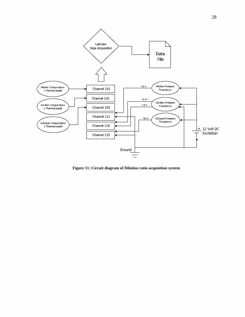
While both the TEOM and the Horiba MEXA-584L provide analog output signals,

the ejector dilutor does not. To make measurements critical to the determination of dilution

ratio, the dilution tunnel was instrumented with thermocouples and pressure transducers on

each inlet and outlet of the ejector to provide temperature and pressure data. Each of these

transducers requires an excitation voltage to be able to output a signal. The data acquisition

for the dilution tunnel was connected according to the schematic in Figure 11.

28

Figure 11: Circuit diagram of Dilution ratio acquisition system

29

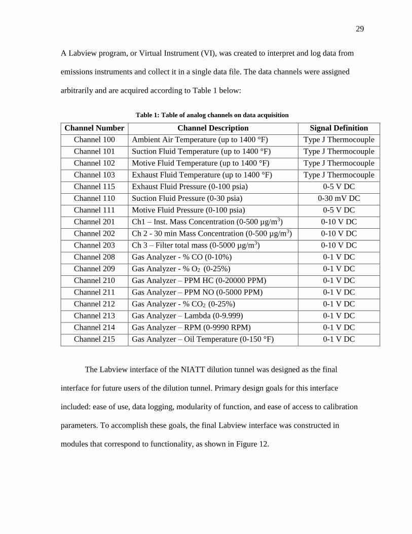
A Labview program, or Virtual Instrument (VI), was created to interpret and log data from

emissions instruments and collect it in a single data file. The data channels were assigned

arbitrarily and are acquired according to Table 1 below:

Table 1: Table of analog channels on data acquisition

Channel Number Channel Description Signal Definition

Channel 100 Ambient Air Temperature (up to 1400 °F) Type J Thermocouple

Channel 101 Suction Fluid Temperature (up to 1400 °F) Type J Thermocouple

Channel 102 Motive Fluid Temperature (up to 1400 °F) Type J Thermocouple

Channel 103 Exhaust Fluid Temperature (up to 1400 °F) Type J Thermocouple

Channel 115 Exhaust Fluid Pressure (0-100 psia) 0-5 V DC

Channel 110 Suction Fluid Pressure (0-30 psia) 0-30 mV DC

Channel 111 Motive Fluid Pressure (0-100 psia) 0-5 V DC

Channel 201 Ch1 – Inst. Mass Concentration (0-500 µg/m3) 0-10 V DC

Channel 202 Ch 2 - 30 min Mass Concentration (0-500 µg/m3) 0-10 V DC

Channel 203 Ch 3 – Filter total mass (0-5000 µg/m3) 0-10 V DC

Channel 208 Gas Analyzer - % CO (0-10%) 0-1 V DC

Channel 209 Gas Analyzer - % O2 (0-25%) 0-1 V DC

Channel 210 Gas Analyzer – PPM HC (0-20000 PPM) 0-1 V DC

Channel 211 Gas Analyzer – PPM NO (0-5000 PPM) 0-1 V DC

Channel 212 Gas Analyzer - % CO2 (0-25%) 0-1 V DC

Channel 213 Gas Analyzer – Lambda (0-9.999) 0-1 V DC

Channel 214 Gas Analyzer – RPM (0-9990 RPM) 0-1 V DC

Channel 215 Gas Analyzer – Oil Temperature (0-150 °F) 0-1 V DC

The Labview interface of the NIATT dilution tunnel was designed as the final

interface for future users of the dilution tunnel. Primary design goals for this interface

included: ease of use, data logging, modularity of function, and ease of access to calibration

parameters. To accomplish these goals, the final Labview interface was constructed in

modules that correspond to functionality, as shown in Figure 12.

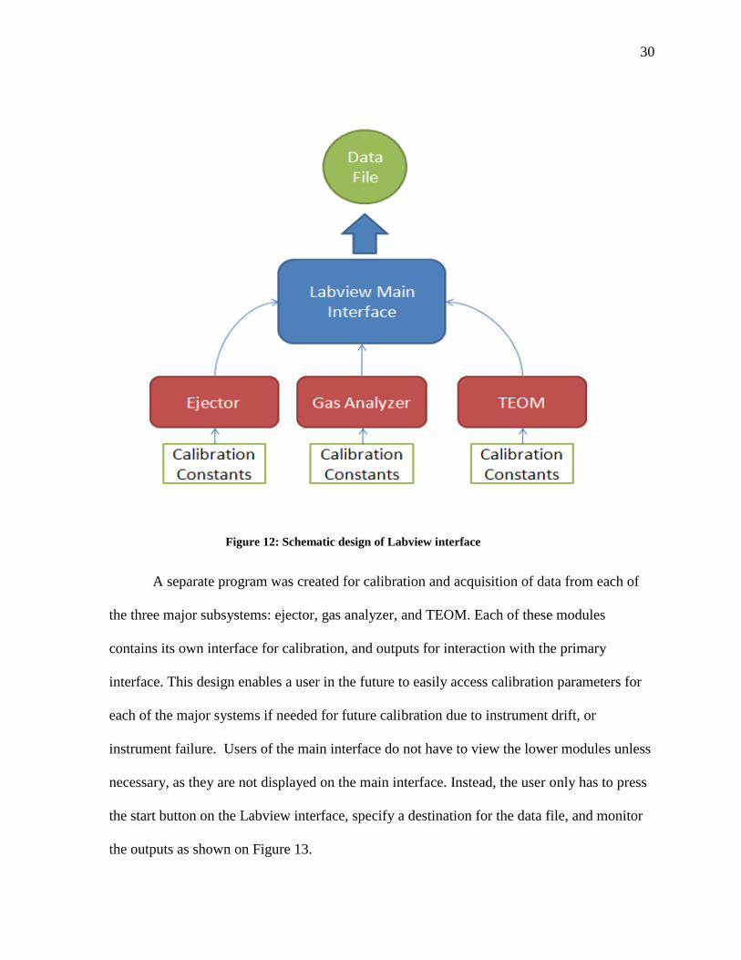
30

A separate program was created for calibration and acquisition of data from each of

the three major subsystems: ejector, gas analyzer, and TEOM. Each of these modules

contains its own interface for calibration, and outputs for interaction with the primary

interface. This design enables a user in the future to easily access calibration parameters for

each of the major systems if needed for future calibration due to instrument drift, or

instrument failure. Users of the main interface do not have to view the lower modules unless

necessary, as they are not displayed on the main interface. Instead, the user only has to press

the start button on the Labview interface, specify a destination for the data file, and monitor

the outputs as shown on Figure 13.

Figure 12: Schematic design of Labview interface

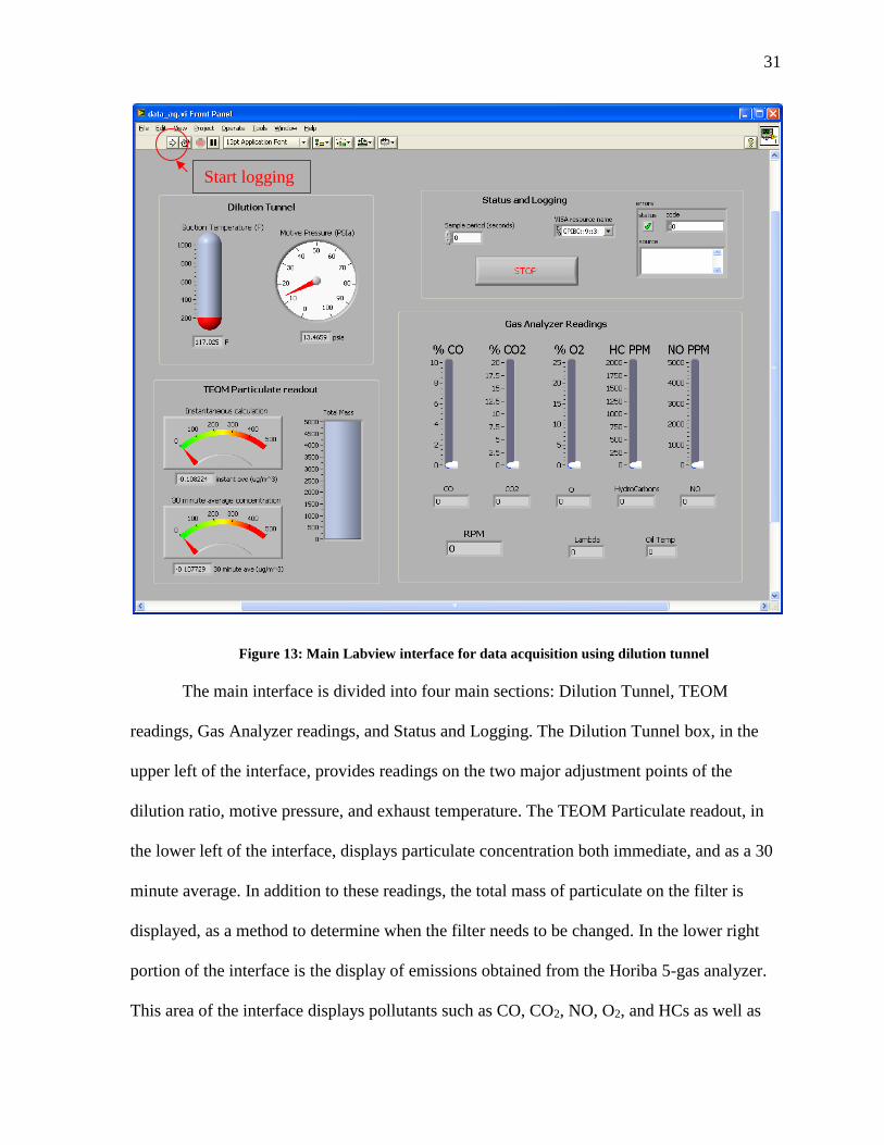
31

The main interface is divided into four main sections: Dilution Tunnel, TEOM

readings, Gas Analyzer readings, and Status and Logging. The Dilution Tunnel box, in the

upper left of the interface, provides readings on the two major adjustment points of the

dilution ratio, motive pressure, and exhaust temperature. The TEOM Particulate readout, in

the lower left of the interface, displays particulate concentration both immediate, and as a 30

minute average. In addition to these readings, the total mass of particulate on the filter is

displayed, as a method to determine when the filter needs to be changed. In the lower right

portion of the interface is the display of emissions obtained from the Horiba 5-gas analyzer.

This area of the interface displays pollutants such as CO, CO2, NO, O2, and HCs as well as

Figure 13: Main Labview interface for data acquisition using dilution tunnel

Start logging

32

the calculated parameter Lambda. Additionally, if the Horiba is connected to the inductive

RPM sensor, or oil temp sensor, the interface will display this data as well.

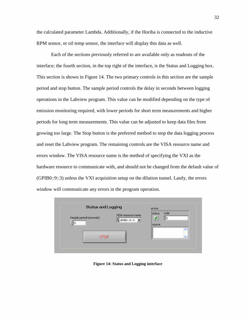
Each of the sections previously referred to are available only as readouts of the

interface; the fourth section, in the top right of the interface, is the Status and Logging box.

This section is shown in Figure 14. The two primary controls in this section are the sample

period and stop button. The sample period controls the delay in seconds between logging

operations in the Labview program. This value can be modified depending on the type of

emission monitoring required, with lower periods for short term measurements and higher

periods for long term measurements. This value can be adjusted to keep data files from

growing too large. The Stop button is the preferred method to stop the data logging process

and reset the Labview program. The remaining controls are the VISA resource name and

errors window. The VISA resource name is the method of specifying the VXI as the

hardware resource to communicate with, and should not be changed from the default value of

(GPIB0::9::3) unless the VXI acquisition setup on the dilution tunnel. Lastly, the errors

window will communicate any errors in the program operation.

Figure 14: Status and Logging interface

33

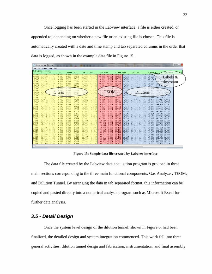
Once logging has been started in the Labview interface, a file is either created, or

appended to, depending on whether a new file or an existing file is chosen. This file is

automatically created with a date and time stamp and tab separated columns in the order that

data is logged, as shown in the example data file in Figure 15.

Figure 15: Sample data file created by Labview interface

The data file created by the Labview data acquisition program is grouped in three

main sections corresponding to the three main functional components: Gas Analyzer, TEOM,

and Dilution Tunnel. By arranging the data in tab separated format, this information can be

copied and pasted directly into a numerical analysis program such as Microsoft Excel for

further data analysis.

3.5 - Detail Design

Once the system level design of the dilution tunnel, shown in Figure 6, had been

finalized, the detailed design and system integration commenced. This work fell into three

general activities: dilution tunnel design and fabrication, instrumentation, and final assembly

5 Gas

Analyzer

TEOM Dilution

Tunnel

Labels &

timestam

p

34

and integration. Dilution tunnel fabrication encompassed the physical design and fabrication

of the dilution tunnel apparatus. Once the apparatus was constructed, instrumentation of the

tunnel was undertaken to place sensors and controls for the instrument. As the final stage of

detail design, the apparatus was assembled in a single cart, with all operating components

onboard, and all controls integrated into a functional platform for engine testing.

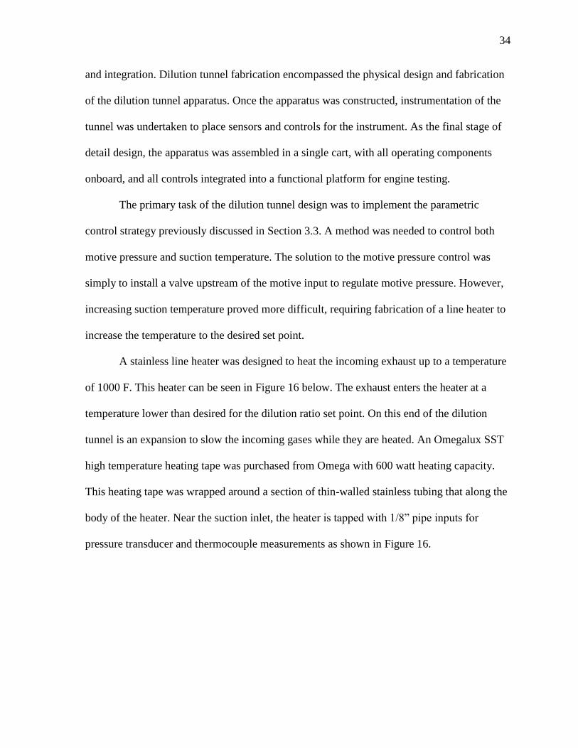
The primary task of the dilution tunnel design was to implement the parametric

control strategy previously discussed in Section 3.3. A method was needed to control both

motive pressure and suction temperature. The solution to the motive pressure control was

simply to install a valve upstream of the motive input to regulate motive pressure. However,

increasing suction temperature proved more difficult, requiring fabrication of a line heater to

increase the temperature to the desired set point.

A stainless line heater was designed to heat the incoming exhaust up to a temperature

of 1000 F. This heater can be seen in Figure 16 below. The exhaust enters the heater at a

temperature lower than desired for the dilution ratio set point. On this end of the dilution

tunnel is an expansion to slow the incoming gases while they are heated. An Omegalux SST

high temperature heating tape was purchased from Omega with 600 watt heating capacity.

This heating tape was wrapped around a section of thin-walled stainless tubing that along the

body of the heater. Near the suction inlet, the heater is tapped with 1/8” pipe inputs for

pressure transducer and thermocouple measurements as shown in Figure 16.

35

Figure 16: Line heater design with temperature and pressure sensor.

Due to the high temperature of the exhaust in the line heater (as high as 1200° F), it

was necessary to place the pressure transducer away from the heater. This was accomplished

using an “S” shaped stainless steel pressure tap, which kept the pressure transducer below its

rated temperature of 450° F, while still allowing accurate pressure measurements.

Additionally, due to the high temperatures, the line heater was surrounded with alumina

silica ceramic fiber insulation for safety reasons.

Early testing on the ejector dilutor revealed that back pressure has a large effect on

dilution ratio. As a result of this testing, care was taken to prevent back pressure downstream

from the ejector dilutor. Each fitting was tapered inside with low angles to prevent pressure

loss and flow separation. Fittings were added to allow the diluted flow to expand into the

sampling chamber and contract to exit into an exhaust handling system. Barbed hose fittings

36

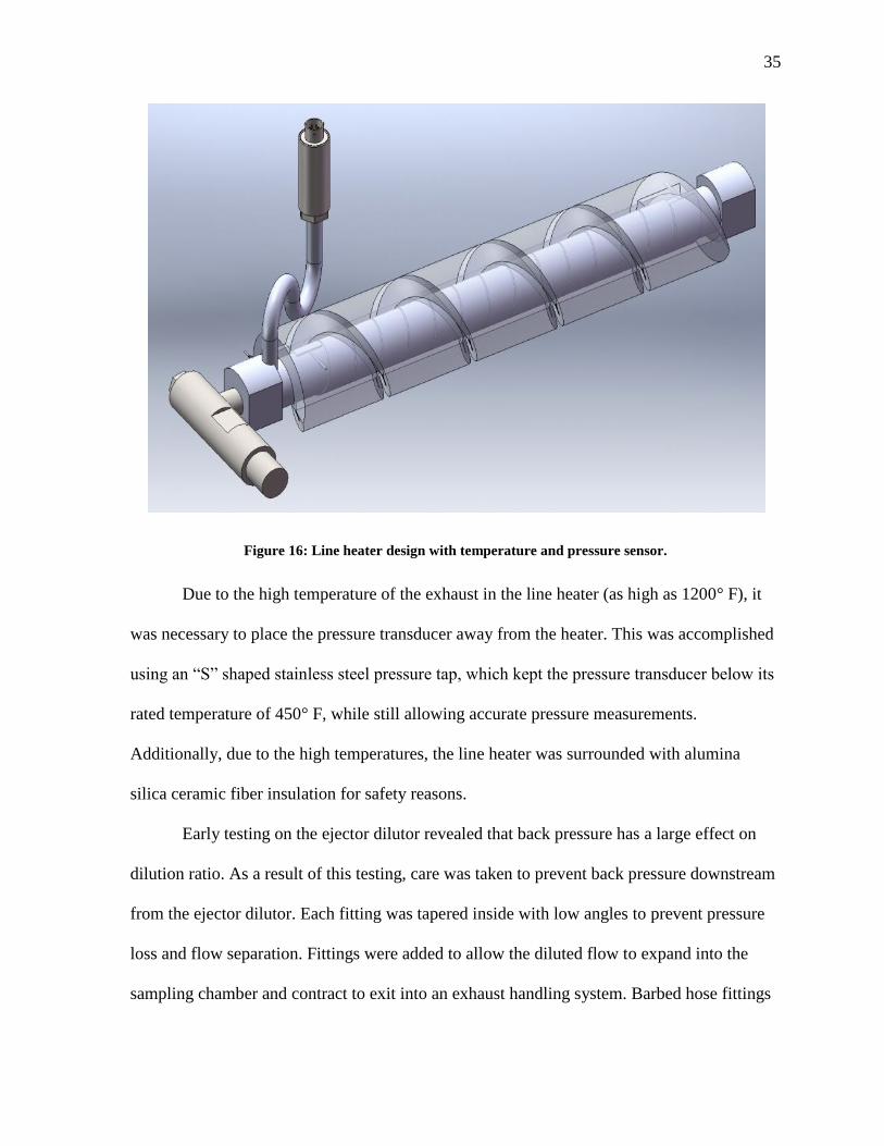
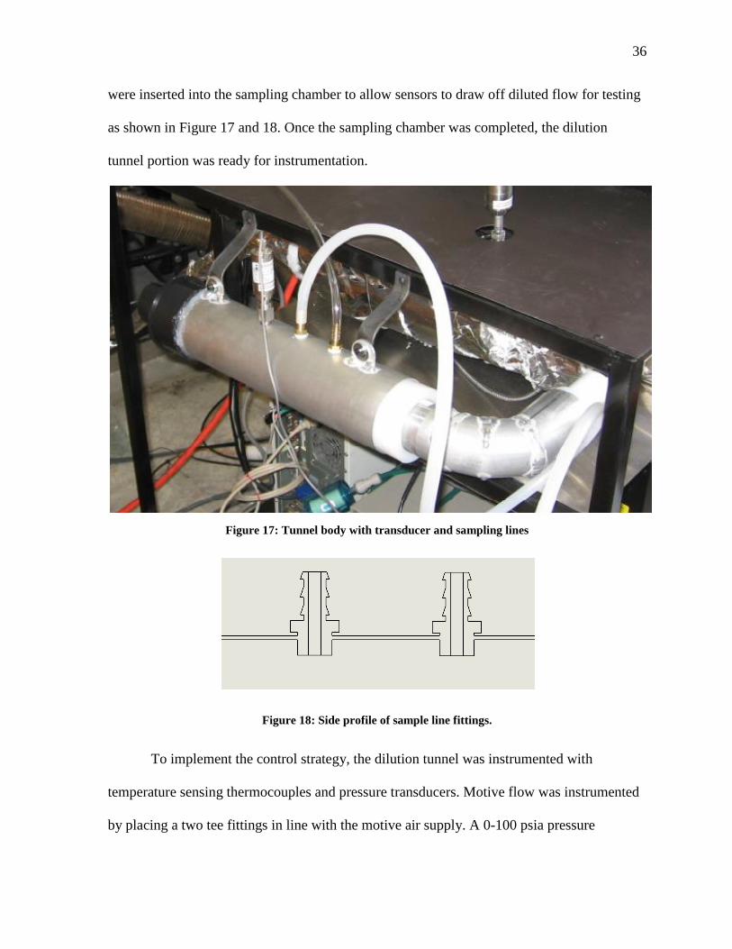
were inserted into the sampling chamber to allow sensors to draw off diluted flow for testing

as shown in Figure 17 and 18. Once the sampling chamber was completed, the dilution

tunnel portion was ready for instrumentation.

Figure 17: Tunnel body with transducer and sampling lines

Figure 18: Side profile of sample line fittings.

To implement the control strategy, the dilution tunnel was instrumented with

temperature sensing thermocouples and pressure transducers. Motive flow was instrumented

by placing a two tee fittings in line with the motive air supply. A 0-100 psia pressure

37

transducer was connected to one of the tee fittings, while a J type thermocouple was

connected to the other. As previously discussed, the suction temperature and pressure were

instrumented by drilling and tapping directly into the fabricated line heater to add a

thermocouple fitting and pressure tap. A 0-30 psia, high temperature, pressure transducer was

attached to the top of the pressure tap. Lastly, the sampling chamber was instrumented with

another 100 psia pressure transducer and J type thermocouple to provide data on the dilution

stream. A 12 volt power supply was connected to the three pressure transducers to provide

excitation voltage as shown in Figure 11 above. These sensors were connected to the VXI

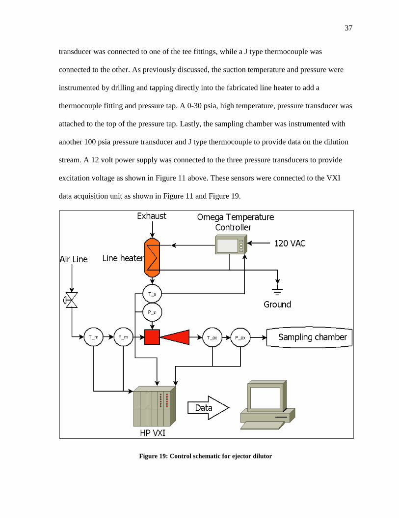
data acquisition unit as shown in Figure 11 and Figure 19.

Figure 19: Control schematic for ejector dilutor

38

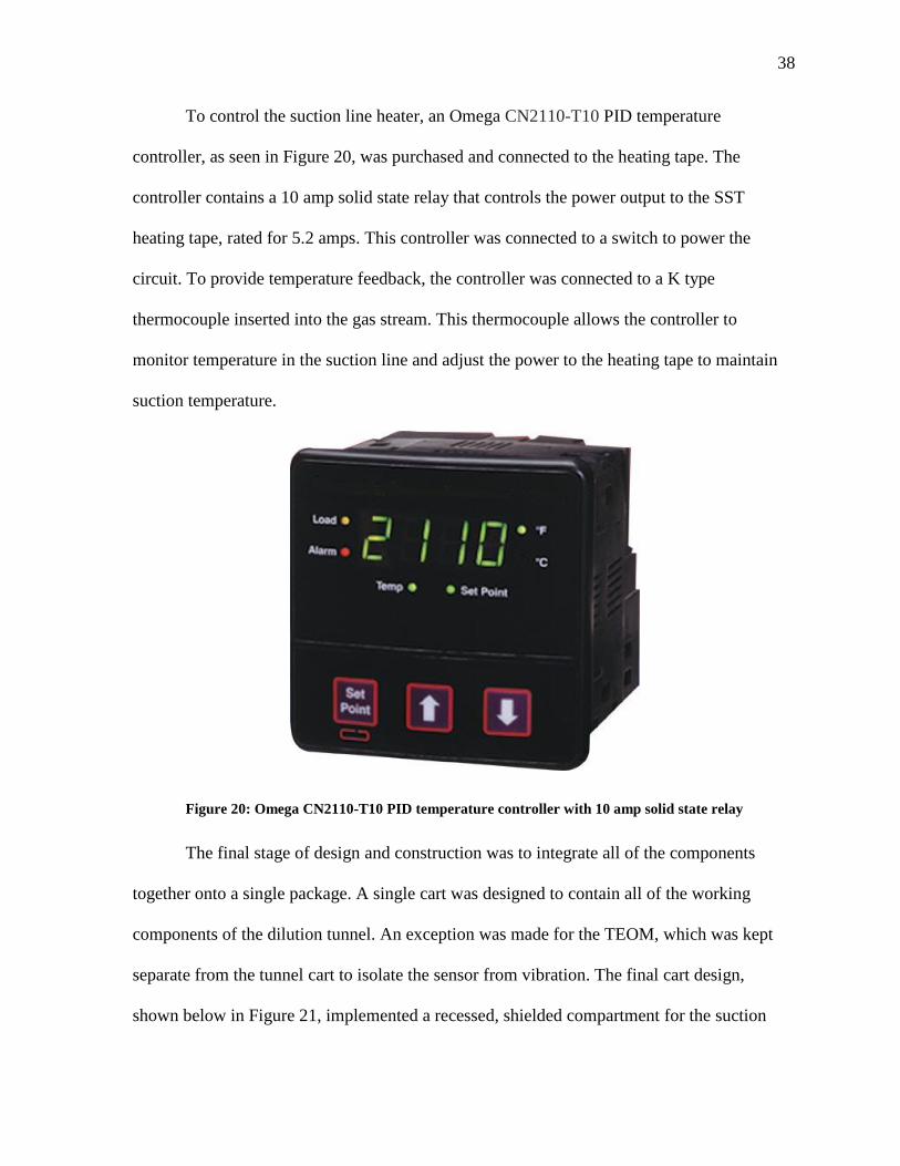
To control the suction line heater, an Omega CN2110-T10 PID temperature

controller, as seen in Figure 20, was purchased and connected to the heating tape. The

controller contains a 10 amp solid state relay that controls the power output to the SST

heating tape, rated for 5.2 amps. This controller was connected to a switch to power the

circuit. To provide temperature feedback, the controller was connected to a K type

thermocouple inserted into the gas stream. This thermocouple allows the controller to

monitor temperature in the suction line and adjust the power to the heating tape to maintain

suction temperature.

Figure 20: Omega CN2110-T10 PID temperature controller with 10 amp solid state relay

The final stage of design and construction was to integrate all of the components

together onto a single package. A single cart was designed to contain all of the working

components of the dilution tunnel. An exception was made for the TEOM, which was kept

separate from the tunnel cart to isolate the sensor from vibration. The final cart design,

shown below in Figure 21, implemented a recessed, shielded compartment for the suction

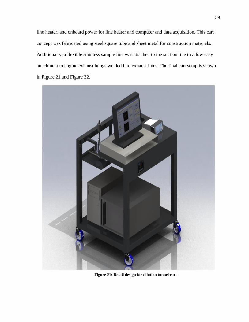
39

line heater, and onboard power for line heater and computer and data acquisition. This cart

concept was fabricated using steel square tube and sheet metal for construction materials.

Additionally, a flexible stainless sample line was attached to the suction line to allow easy

attachment to engine exhaust bungs welded into exhaust lines. The final cart setup is shown

in Figure 21 and Figure 22.

Figure 21: Detail design for dilution tunnel cart

40

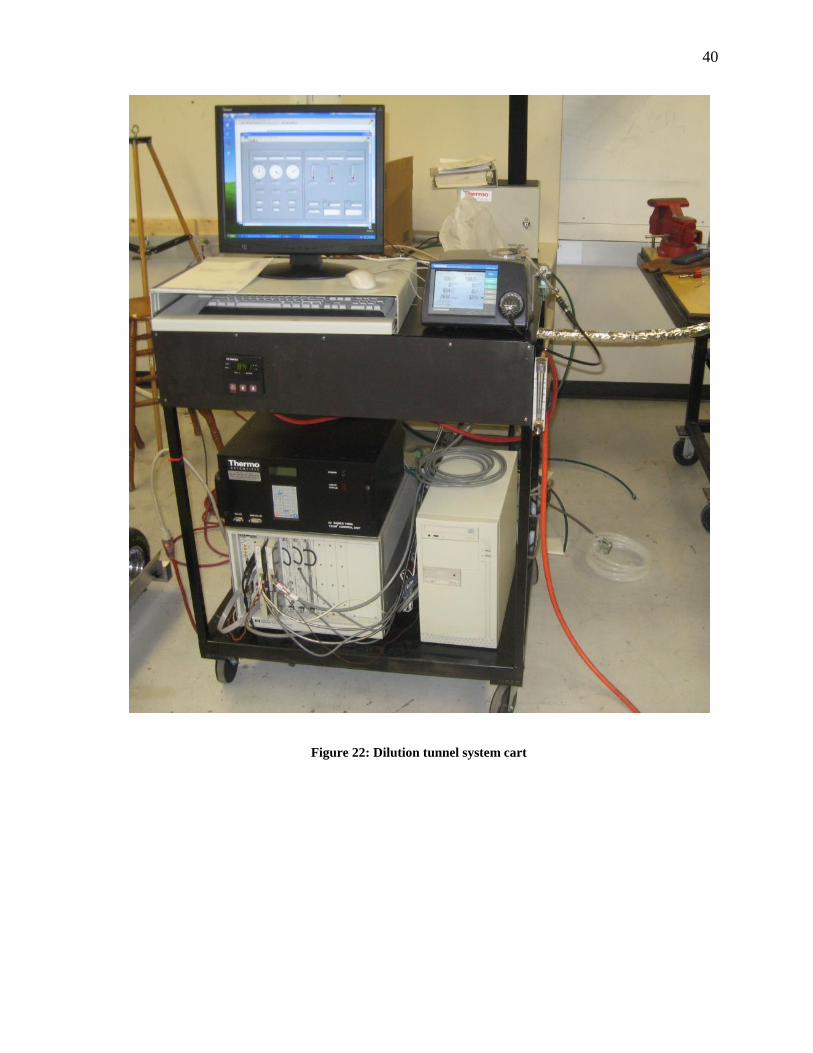
Figure 22: Dilution tunnel system cart

41

Chapter 4: Dilution Tunnel Validation

4.1 - Dilution Device Calibration

Arguably the most important measurement in a dilution tunnel is that of the dilution

ratio. Error in the dilution ratio serves to magnify error in other instruments, such that at a

certain level of uncertainty, the measurements would be almost useless. To calibrate the

dilution device, several tests were performed to correlate temperature and pressure

measurements around the ejector pump with overall dilution ratio through the dilution tunnel

as described in Section 3.3. Ideally, this calibration would result in an overall equation or

curve-fit for dilution ratio as a function of exhaust temperature and motive pressure as

previously described in section 3.2. However, when initial testing commenced, it became

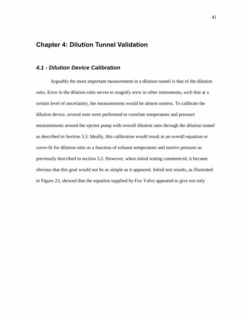
obvious that this goal would not be as simple as it appeared. Initial test results, as illustrated

in Figure 23, showed that the equation supplied by Fox Valve appeared to give not only

42

different answers for the dilution ratio as measured by rotameter flow meters, but the trend of

dilution ratios between the calculation methods diverged considerably.

Figure 23: Dilution ratios at three different set points as calculated by two different methods

To resolve the issues with determining dilution ratio, a simpler and more robust test

was conceived to determine dilution ratio. The suction of the ejector was connected to a

supply of nearly pure CO2 (99+%) at atmospheric pressure and allowed to draw the CO2 in,

the same way the ejector would sample exhaust. On the exhaust of the ejector, the Horiba

MEXA-584L was positioned to sample the diluted stream. Since the MEXA was calibrated

to ignore atmospheric levels of carbon dioxide, any CO2 detected in the diluted stream would

have been introduced to the stream via the ejector suction. By taking a volumetric

measurement of the concentration of CO2, the dilution ratio could be backed out using the

following simple equation:

0

2

4

6

8

10

12

14

16

18

0 psia 10 psia 20 psia 30 psia 40 psia 50 psia 60 psia

Fox Valve Calculation

Rotameter data

43

𝐷𝑟 = 1/(%𝐶𝑂2)

This test setup proved to be much simpler and more accurate than previous methods due to

the level of accuracy of the 5 gas analyzer.

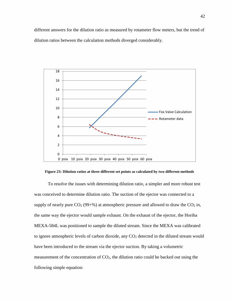
During the CO2 cal-gas dilution calibration, a number of constant temperature

sweeps, and constant pressure sweeps were performed and plotted as a function of dilution

ratio. The collected data can be seen in Figure 24 and Figure 25. One notable element of the

data obtained using this method was that it did not substantiate any of the previous methods

for measuring dilution ratio. However, unlike the previous data, the data obtained using CO2

cal-gas dilution was both repeatable and, as shown later, fairly accurate.

Figure 24: Dilution ratio as a function of suction temperature with constant motive pressure measured

with CO2 cal-gas dilution

8

9

10

11

12

13

14

15

16

17

300 F 350 F 400 F 450 F 500 F 550 F 600 F 650 F 700 F 750 F

30 psia

40 psia

50 psia

60 psia

44

Figure 24 is the raw data obtained using CO2 cal-gas dilution, varying temperature

while holding motive pressures constant. This data was obtained by heating the suction

temperature to a 700 F, turning off the line heater, and logging data as the dilution tunnel

cooled down. This data showed common trends of dilution ratios between data sets, and

demonstrated the dilution ratio’s low sensitivity to temperature shifts. Each set of data

showed at most a shift of 1 point of dilution ratio per hundred degrees of temperature change.

Figure 25: Dilution ratio as a function of motive pressure with constant temperature data sets measured

using CO2 cal-gas dilution

Figure 25 is data obtained using CO2 cal-gas dilution, at constant temperatures while

varying the motive pressures. This data was obtained by setting the suction temperature to a

constant point, and varying the motive pressure while logging dilution ratios. This data

8

9

10

11

12

13

14

15

16

17

10 psia 20 psia 30 psia 40 psia 50 psia 60 psia 70 psia

200 F

300 F

400 F

500 F

600 F

700F

45

showed good correlation between different temperatures, and demonstrated the dilution

ratio’s high sensitivity to changing motive pressure. The dilution ratio at a given temperature

was seen to vary approximately 5 points over a moderate pressure change of only 40 psi.

These results validated the control scheme of using the motive pressure and suction

temperature as “coarse” and “fine” control respectively.

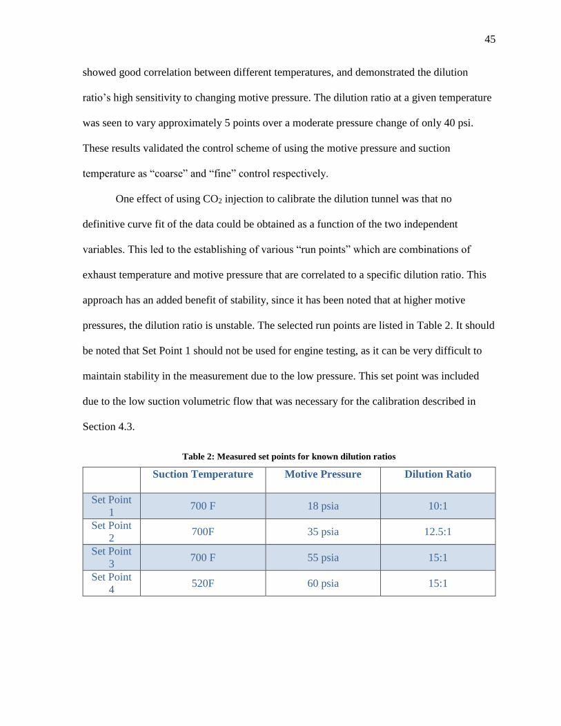
One effect of using CO2 injection to calibrate the dilution tunnel was that no

definitive curve fit of the data could be obtained as a function of the two independent

variables. This led to the establishing of various “run points” which are combinations of

exhaust temperature and motive pressure that are correlated to a specific dilution ratio. This

approach has an added benefit of stability, since it has been noted that at higher motive

pressures, the dilution ratio is unstable. The selected run points are listed in Table 2. It should

be noted that Set Point 1 should not be used for engine testing, as it can be very difficult to

maintain stability in the measurement due to the low pressure. This set point was included

due to the low suction volumetric flow that was necessary for the calibration described in

Section 4.3.

Table 2: Measured set points for known dilution ratios

Suction Temperature Motive Pressure Dilution Ratio

Set Point

1 700 F 18 psia 10:1

Set Point

2 700F 35 psia 12.5:1

Set Point

3 700 F 55 psia 15:1

Set Point

4 520F 60 psia 15:1

46

4.2 - Labview Calibration

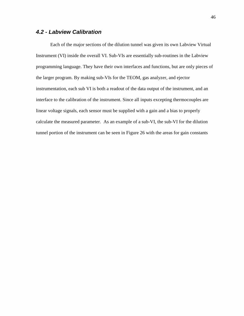
Each of the major sections of the dilution tunnel was given its own Labview Virtual

Instrument (VI) inside the overall VI. Sub-VIs are essentially sub-routines in the Labview

programming language. They have their own interfaces and functions, but are only pieces of

the larger program. By making sub-VIs for the TEOM, gas analyzer, and ejector

instrumentation, each sub VI is both a readout of the data output of the instrument, and an

interface to the calibration of the instrument. Since all inputs excepting thermocouples are

linear voltage signals, each sensor must be supplied with a gain and a bias to properly

calculate the measured parameter. As an example of a sub-VI, the sub-VI for the dilution

tunnel portion of the instrument can be seen in Figure 26 with the areas for gain constants

47

and bias constants highlighted.

Figure 26: Sub-VI for calibration of the dilution tunnel sensors with gain and bias constants highlighted.

Determining calibration constants was accomplished by direct measurement or by

using calibration data supplied by the manufacturer. Gain was determined by dividing the full

scale measurement by the full scale signal voltage. For example, a pressure transducer with a

range of 0-100 psia and an output of 0-5 volts DC will have a gain of (100/5=20). Once gain

was specified, bias was determined by measuring the signal at zero output and adjusting the

bias until the sensor reads zero. For example if exhaust pressure reads 15 psia, the bias would

be 1.6 psia to bring the sensor to the correct ambient pressure of 13.4 psia. Once the

calibration constants are specified, the VXI will measure DC voltage across the sensor,

Gain constants

Bias constants

48

multiply the voltage by the gain, and then subtract the bias to get a measurement of pressure

in units of psia.

Although not pictured here, the sub VIs for both the gas analyzer and TEOM have

nearly identical interfaces, and have been designed to work the same way as the interface

shown in Figure 26. These interfaces can be found in Appendix B. The rationale for making

these constants accessible through the Labview interface was to make recalibration easier.

Recalibrations will not need to occur often, but over long periods of time, sensor outputs will

often “drift”, necessitating recalibration.

4.3 - Bench Testing with Calibration Gas

Upon completion of calibration, the dilution tunnel system as a whole needed to be

tested to validate that it not only works as it is supposed to, but also provides accurate and

repeatable data to the user. Validation procedure consisted of two separate trials: calibration

gas validation, and dynamic engine validation.

Calibration gas, or cal-gas, bench testing was the first form of validation to be

conducted on the NIATT dilution tunnel. The process of cal-gas validation is to introduce

pure cal-gas into the suction port of the dilution tunnel and compare the measured

concentrations as measured by the gas analyzer of the dilution tunnel. This process is

compared to the results as the cal-gas is measured un-diluted by the gas analyzer. Given a

known dilution ratio, these measurements should correlate well if the tunnel is working

correctly.

To conduct the cal-gas validation, several containers of calibration gas were chosen

from stores available to the Small Engine Research Facility. Four separate containers of cal-

gas were chosen from the stores of SMERF for both their general spread of pollutant species,

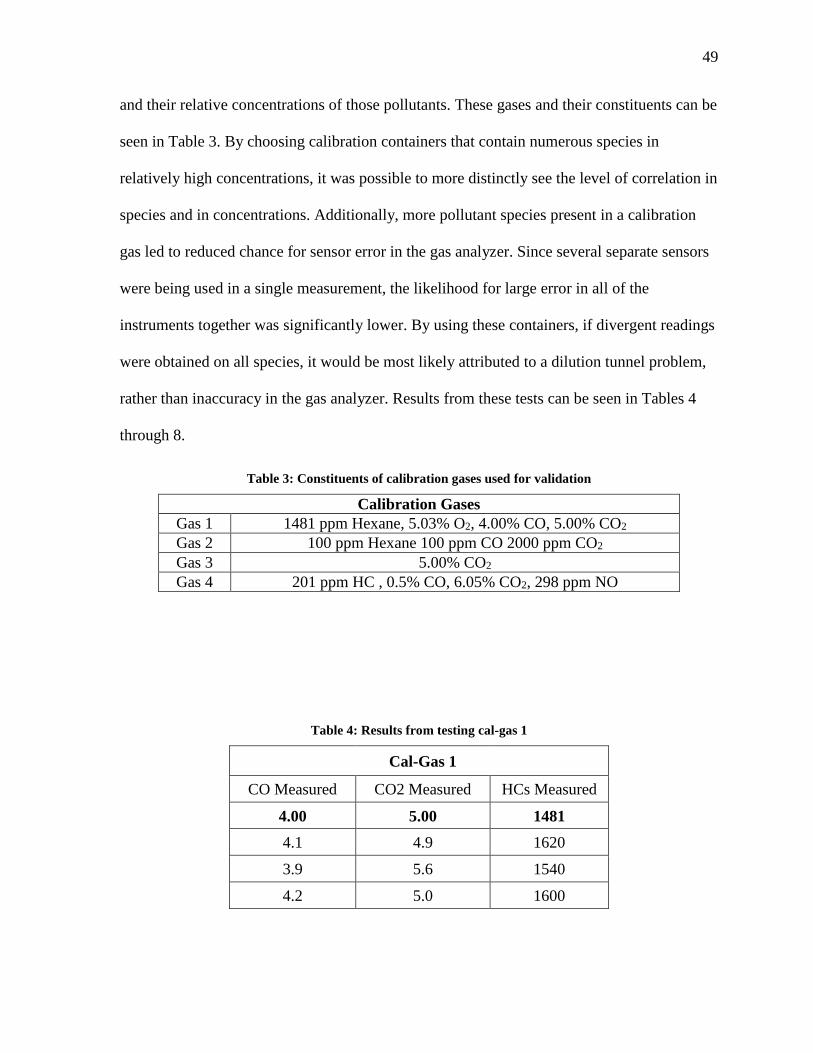
49

and their relative concentrations of those pollutants. These gases and their constituents can be

seen in Table 3. By choosing calibration containers that contain numerous species in

relatively high concentrations, it was possible to more distinctly see the level of correlation in

species and in concentrations. Additionally, more pollutant species present in a calibration

gas led to reduced chance for sensor error in the gas analyzer. Since several separate sensors

were being used in a single measurement, the likelihood for large error in all of the

instruments together was significantly lower. By using these containers, if divergent readings

were obtained on all species, it would be most likely attributed to a dilution tunnel problem,

rather than inaccuracy in the gas analyzer. Results from these tests can be seen in Tables 4

through 8.

Table 3: Constituents of calibration gases used for validation

Calibration Gases

Gas 1 1481 ppm Hexane, 5.03% O2, 4.00% CO, 5.00% CO2

Gas 2 100 ppm Hexane 100 ppm CO 2000 ppm CO2

Gas 3 5.00% CO2

Gas 4 201 ppm HC , 0.5% CO, 6.05% CO2, 298 ppm NO

Table 4: Results from testing cal-gas 1

Cal-Gas 1

CO Measured CO2 Measured HCs Measured

4.00 5.00 1481

4.1 4.9 1620

3.9 5.6 1540

4.2 5.0 1600

50

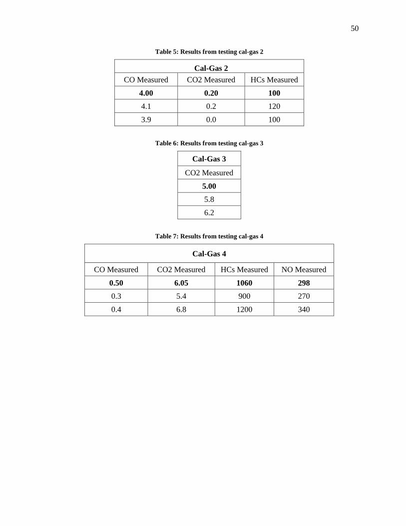
Table 5: Results from testing cal-gas 2

Cal-Gas 2

CO Measured CO2 Measured HCs Measured

4.00 0.20 100

4.1 0.2 120

3.9 0.0 100

Table 6: Results from testing cal-gas 3

Cal-Gas 3

CO2 Measured

5.00

5.8

6.2

Table 7: Results from testing cal-gas 4

Cal-Gas 4

CO Measured CO2 Measured HCs Measured NO Measured

0.50 6.05 1060 298

0.3 5.4 900 270

0.4 6.8 1200 340

51

Results from cal-gas testing were varied. Calibration gas #2 in particular generated

very poor results. This was primarily because the calibration gas had very low mass per unit

volume of pollutants: 100 ppm HC, 0.01% CO, and 0.2% CO2. Once diluted, the

concentrations should look something like 10 ppm HC, 0.001% CO and 0.02% CO2. This

makes it unlikely that any reasonable degree of accuracy could be expected on this

measurement, as it pushes the resolution of the gas analyzer beyond its accuracy limits.

However, this data was important as an example of limitations of the dilution tunnel.

One limitation that likely inhibited more accurate readings was the sample rate. Cal-

gas is highly expensive, and the containers of gases available for testing were fairly small.

Additionally, the regulator for these gases was only able to supply up to 6 L/min of cal-gas

for testing. This meant not only that allowing the analyzer to fully stabilize would involve

using an entire container of cal-gas, but additionally meant that only dilution ratios that did

not sample more than 6 L/min of suction gas could be tested with these gases. The exception

to this was calibration gas #4, which was in a larger tank held at higher pressure and could be

sampled longer and at other set points. Consequently, cal-gas validation could only be used

to establish the general validity of the CO2 cal-gas dilution ratios established.

4.4 – Engine Testing

As final validation of the dilution tunnel apparatus, testing was performed using an

actual engine platform. This procedure consisted of connecting the dilution tunnel to a

Volkswagen 1.9 L TDI diesel engine to provide a real operating scenario. The engine was set

at a specific RPM and loaded using an alternator and set of resistor banks; this setup can be

seen in Figure 27 . While maintaining that specific load point of the engine, raw exhaust

emissions were measured using the Horiba 5 gas analyzer. Once the readings had stabilized,

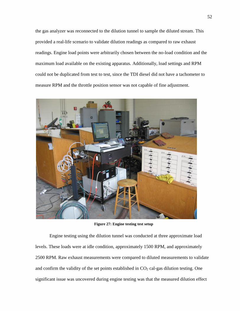
52

the gas analyzer was reconnected to the dilution tunnel to sample the diluted stream. This

provided a real-life scenario to validate dilution readings as compared to raw exhaust

readings. Engine load points were arbitrarily chosen between the no-load condition and the

maximum load available on the existing apparatus. Additionally, load settings and RPM

could not be duplicated from test to test, since the TDI diesel did not have a tachometer to

measure RPM and the throttle position sensor was not capable of fine adjustment.

Figure 27: Engine testing test setup

Engine testing using the dilution tunnel was conducted at three approximate load

levels. These loads were at idle condition, approximately 1500 RPM, and approximately

2500 RPM. Raw exhaust measurements were compared to diluted measurements to validate

and confirm the validity of the set points established in CO2 cal-gas dilution testing. One

significant issue was uncovered during engine testing was that the measured dilution effect

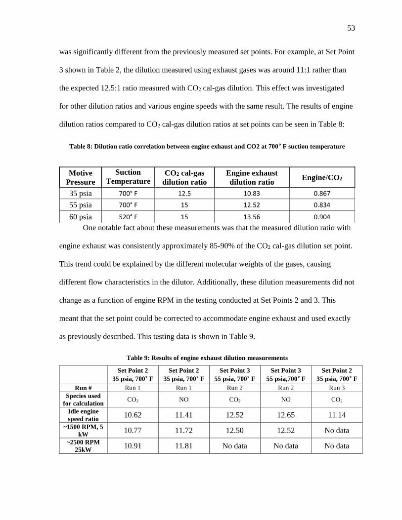
53

was significantly different from the previously measured set points. For example, at Set Point

3 shown in Table 2, the dilution measured using exhaust gases was around 11:1 rather than

the expected 12.5:1 ratio measured with CO2 cal-gas dilution. This effect was investigated

for other dilution ratios and various engine speeds with the same result. The results of engine

dilution ratios compared to CO2 cal-gas dilution ratios at set points can be seen in Table 8:

Table 8: Dilution ratio correlation between engine exhaust and CO2 at 700° F suction temperature

One notable fact about these measurements was that the measured dilution ratio with

engine exhaust was consistently approximately 85-90% of the CO2 cal-gas dilution set point.

This trend could be explained by the different molecular weights of the gases, causing

different flow characteristics in the dilutor. Additionally, these dilution measurements did not

change as a function of engine RPM in the testing conducted at Set Points 2 and 3. This

meant that the set point could be corrected to accommodate engine exhaust and used exactly

as previously described. This testing data is shown in Table 9.

Table 9: Results of engine exhaust dilution measurements

Set Point 2

35 psia, 700° F

Set Point 2

35 psia, 700° F

Set Point 3

55 psia, 700° F

Set Point 3

55 psia,700° F Set Point 2

35 psia, 700° F

Run # Run 1 Run 1 Run 2 Run 2 Run 3

Species used

for calculation CO2 NO CO2 NO CO2

Idle engine

speed ratio 10.62 11.41 12.52 12.65 11.14

~1500 RPM, 5

kW 10.77 11.72 12.50 12.52 No data

~2500 RPM

25kW 10.91 11.81 No data No data No data

Motive

Pressure

Suction

Temperature CO2 cal-gas

dilution ratio

Engine exhaust

dilution ratio Engine/CO2

35 psia 700° F 12.5 10.83 0.867

55 psia 700° F 15 12.52 0.834

60 psia 520° F 15 13.56 0.904

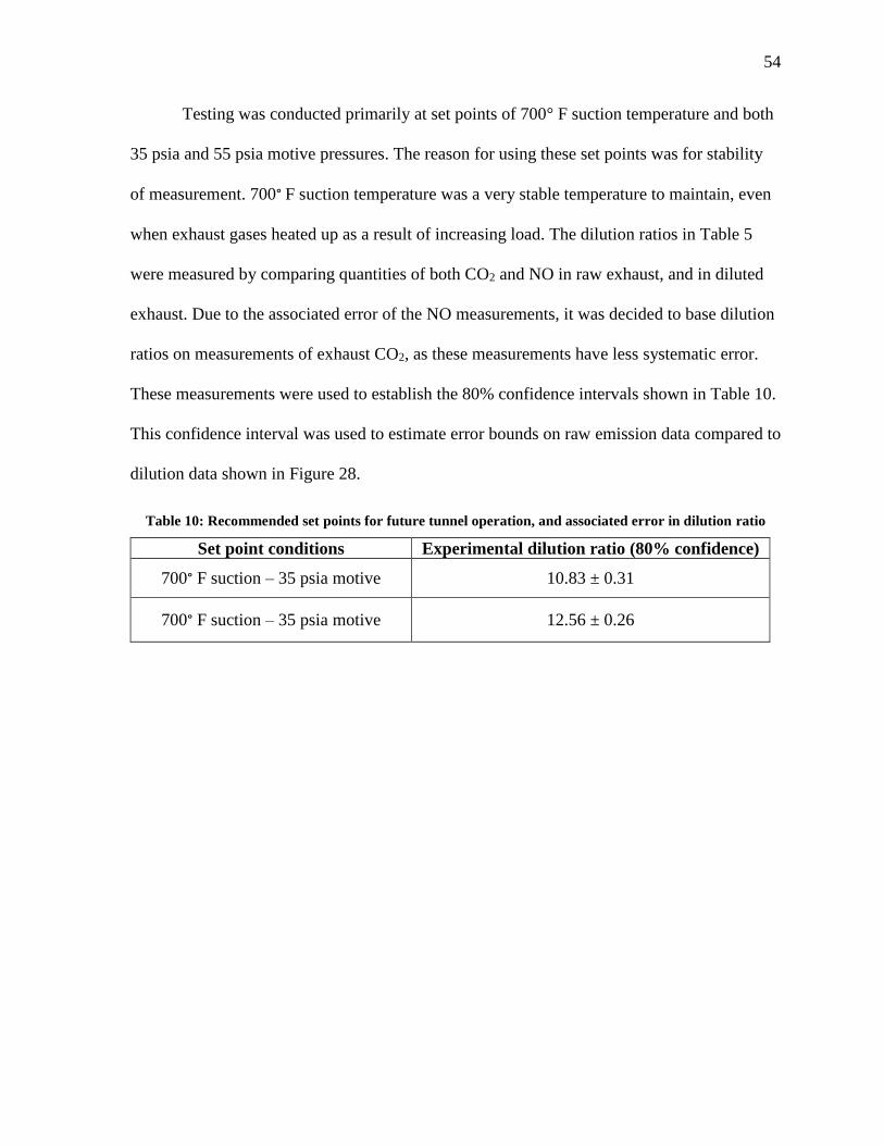
54

Testing was conducted primarily at set points of 700° F suction temperature and both

35 psia and 55 psia motive pressures. The reason for using these set points was for stability

of measurement. 700° F suction temperature was a very stable temperature to maintain, even

when exhaust gases heated up as a result of increasing load. The dilution ratios in Table 5

were measured by comparing quantities of both CO2 and NO in raw exhaust, and in diluted

exhaust. Due to the associated error of the NO measurements, it was decided to base dilution

ratios on measurements of exhaust CO2, as these measurements have less systematic error.

These measurements were used to establish the 80% confidence intervals shown in Table 10.

This confidence interval was used to estimate error bounds on raw emission data compared to

dilution data shown in Figure 28.

Table 10: Recommended set points for future tunnel operation, and associated error in dilution ratio

Set point conditions Experimental dilution ratio (80% confidence)

700° F suction – 35 psia motive 10.83 ± 0.31

700° F suction – 35 psia motive 12.56 ± 0.26

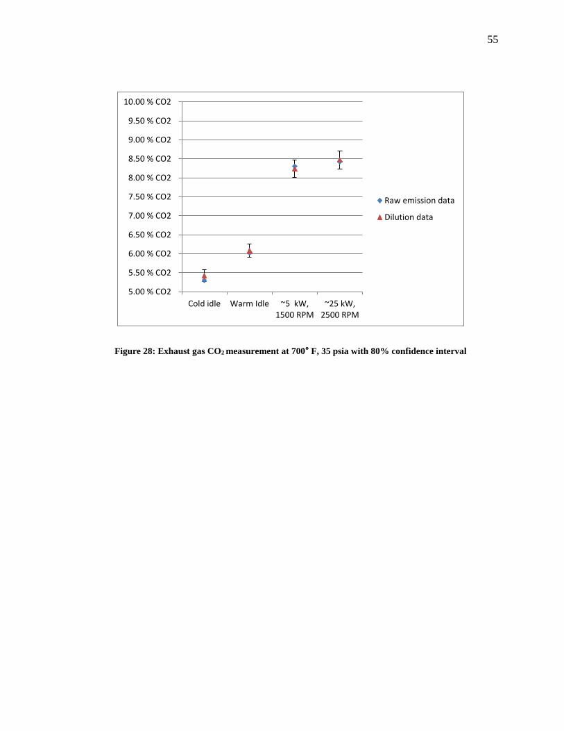
55

Figure 28: Exhaust gas CO2 measurement at 700° F, 35 psia with 80% confidence interval

5.00 % CO2

5.50 % CO2

6.00 % CO2

6.50 % CO2

7.00 % CO2

7.50 % CO2

8.00 % CO2

8.50 % CO2

9.00 % CO2

9.50 % CO2

10.00 % CO2

Cold idle Warm Idle ~5 kW,1500 RPM

~25 kW,2500 RPM

Raw emission data

Dilution data

56

Chapter 5: Conclusions and Recommendations

As designed and fabricated, the NIATT dilution tunnel fulfills all of the design

requirements previously discussed in section 3.1. The system is contained on a portable cart,

making it ideal for the crowded environment of the Small Engine Research Facility at

University of Idaho. It contains one easy-to-use interface that displays and logs all data for

future use. All functions and controls necessary for operation of the dilution tunnel are

located onboard the cart, meaning that the cart only needs to be connected to a power supply

and air line to function. Final tunnel specifications can be found in Table 11. Additionally,

several pictures of the NIATT dilution tunnel can be seen in Figure 29 through Figure 31.

Table 11: NIATT dilution tunnel specifications

Sample chamber volume 2.1 Liters

Diluted exhaust flow 40-150 L/min (dilution ratio dependent)

Particulate sensor flow rate 5-13 Liters/min

Gas analyzer flow rate 4 Liters/min

Residence time 3.2 - .85 seconds (dilution ratio dependent)

Measurement Capabilities HC, CO, CO

2, O

2, NO

x, & Particulate mass

concentration

Particulate Sensor Thermo Scientific TEOM 1400-ab

Gas Analyzer Horiba MEXA-584L w/ NO & O

2

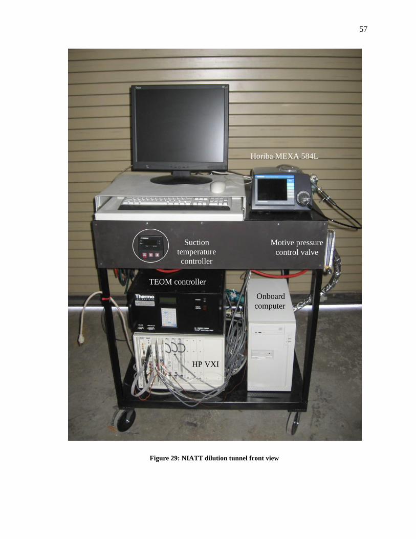
57

Figure 29: NIATT dilution tunnel front view

Suction

temperature

controller

Onboard

computer

HP VXI

TEOM controller

Motive pressure

control valve

Horiba MEXA 584L

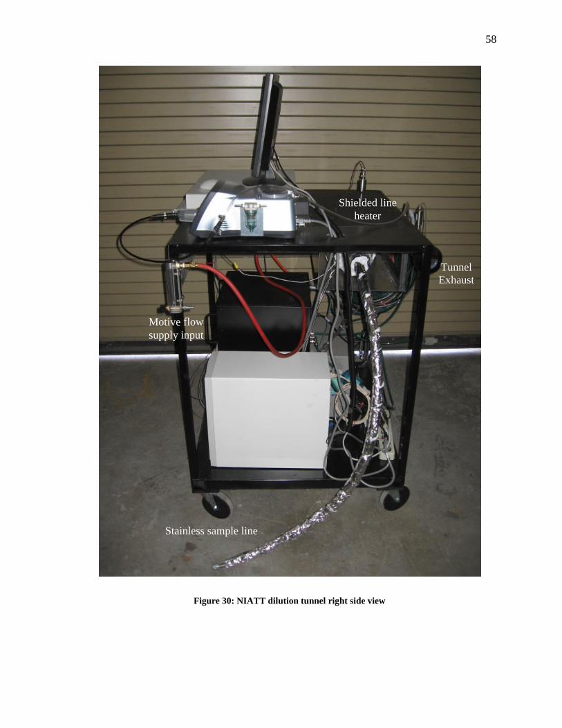
58

Figure 30: NIATT dilution tunnel right side view

Stainless sample line

Shielded line

heater

Motive flow

supply input

Tunnel

Exhaust

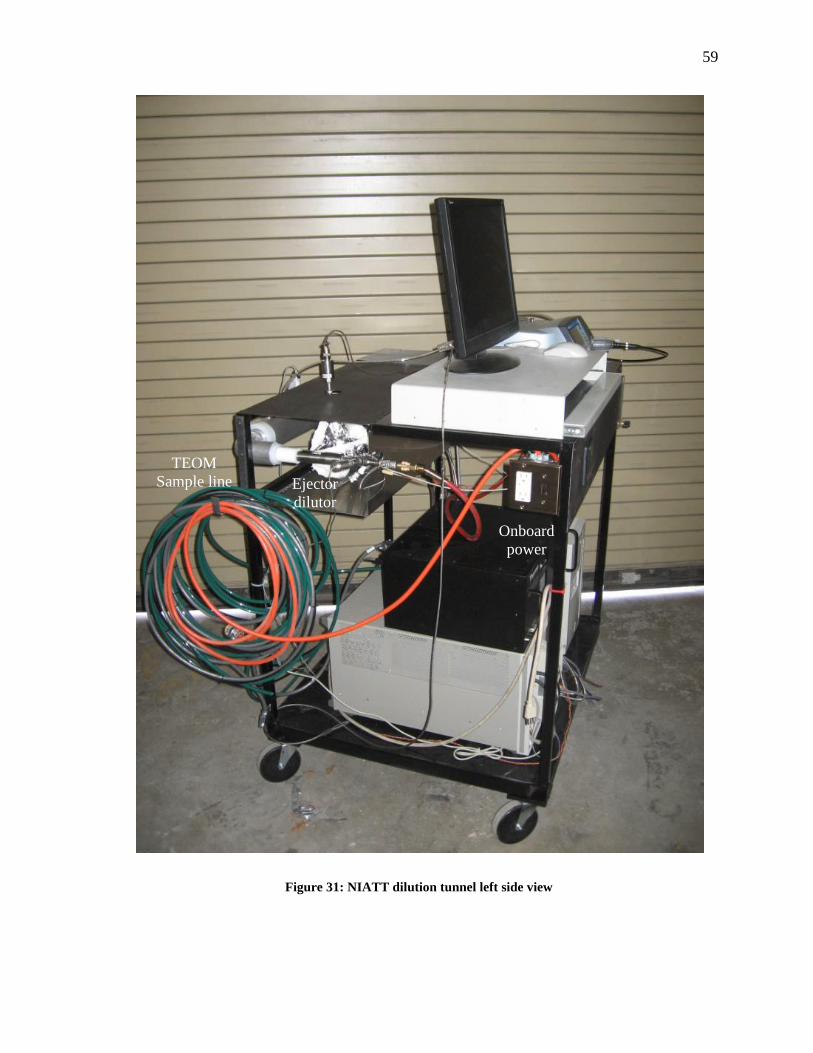
59

Figure 31: NIATT dilution tunnel left side view

Onboard

power

TEOM

Sample line

Ejector

dilutor

60

As discussed in Section 4.4, engine tests revealed two set points that should be used

to set the dilution ratio at the start of testing with the dilution tunnel. Either set point can be

used to good effect, although checking the dilution ratio, as described in Section 4.4 using

raw exhaust comparison, is recommended before testing. These set points correspond to

dilution ratios shown in Table 10, and have experimental error of ± 0.3. This experimental

error was fairly close to the 3.4% root sum squared error based on the dilution ratio equation.

Some lessons were learned in the validation of the dilution tunnel that should be

heeded by future users. For particulate testing, the primary lesson learned was how sensitive

the TEOM is to particulate matter and vibration. Even slight bumps or vibration caused

TEOM readings to fluctuate wildly for almost 5 minutes. Additionally, large quantities of

particulate, such as a diesel engine produces at startup or acceleration, also create

fluctuations in particulate readout that may or may not represent actual measurement of

particles. Regardless of the efficacy of these measurements, the measurements exceed the

scale of the analog output from the TEOM. This scale can be changed, but would drastically

affect resolution of the measured particulate matter. In short, transient particulate testing will

probably not be possible without further development on the dilution tunnel and further

adjustment of the TEOM itself.

Another important lesson learned in engine testing is the necessity of carefully

choosing sampling locations. There are two pitfalls to avoid in choosing an area to place a

sampling port in the exhaust system: exhaust air mixing, and exhaust pressure. Exhaust ports

should be placed at least 18 inches from the atmospheric exit of the exhaust stream to prevent

induction of ambient air from the exhaust exit. Also, care must be taken to avoid pressure

drops downstream of the sampling port. As engine RPM increases, this can cause back

61

pressure in the exhaust system that could pressurize the suction line. This can be eliminated

by making sure that the exhaust is sampled shortly before it exits to atmosphere. If this is not

possible, the pressure could be removed by installing a manual valve on the suction line, and

creating enough pressure drop in the exhaust line to bring the suction pressure reading down

to atmospheric pressure. However, this would not be desirable, due to the need to adjust this

valve every time the RPM changes.

While the system meets the needs of current testing, there are some areas for

improvement in the next generation. While prolonged usage may reveal more shortcomings,

one of the biggest areas for improvement on the NIATT dilution tunnel is the addition of

better, dedicated analyzers for the primary species of emissions. Ideally these sensors would

be a NDIR sensor for detection of CO, CO2, and HCs, and a dedicated chemiluminescent

sensor for detecting nitrogen oxides, and separate dedicated O2, and H2 sensors. Higher

functionality NDIR sensors can be calibrated to determine relative amounts of various

species of molecule, having the potential to determine quantities of hydrocarbons of different

species than the commonly measured hexane. This may especially be important in the

analysis of emissions from engines combusting alternative fuels such as ethanol or biodiesel.

Furthermore, acquisition of dedicated sensors for NOx, O2, and H2 would expand capabilities

for testing at the university that may only be envisioned in the future.

By purchasing more accurate equipment, it would be possible to attain greater

accuracy in the dilution tunnel. This equipment could also potentially determine deficiencies

in the dilution tunnel apparatus that are not possible to detect using current equipment.

Moreover, separate dedicated sensors would allow for the gradual acquisition of better

equipment as budget allows, rather than as an all-in-one expense.

62

References

[1] Q. Wei, D. Kittleson, W.Watts, Single Stage Dilution Tunnel, SAE Paper 2001-01-0207

[2] Introduction to Internal Combustion Engines, 3rd Ed. Richard Stone, SAE International,

1999

[3] J. Cromas, J. Ghandhi, Lubricating Oil Contribution to Direct-Injection Two Stroke

Engine Particulate Emissions, SAE Paper 2004-32-0012

[4] W. Bachalo, D. Snelling, G. Smallwood, R. Sawchuk, et al, Particulate Matter

Measurements in a Diesel Engine Exhaust by Laser-Induced Incandescence and the

Standard Gravimetric Procedure, SAE Paper 1999-01-3653

[5] M Maricq, R. Chase, D. Podsiadlik, R. Vogt, Vehicle Exhaust Particle Size Distributions:

A Comparison of Tailpipe and Dilution Tunnel Measurements, SAE Paper 1999-01-1461

[6] H. Fukushima, H. Uchihara, et al, An Alternative Technique for Low Particulate

Measurement, SAE Paper 2001-01-0218

[7] D. Okrent, Optimization of a Third Generation TEOM Monitor for Measuring Diesel

Particulate in Real Time, SAE Paper 980409

[8] Thermo Scientific Ambient Particulate Monitor, TEOM 1400ab; Continuous mass

measurement of particulate matter in ambient air (2009) [Brochure]. Thermo Fisher

Scientific Inc.

[9] D. Podsiadlik, R. Chase, D. Lewis, M. Spears, Phase-based TEOM Measurements

Compared with Traditional Filters for Diesel PM, SAE Paper 2003-01-0783

[10] S. Xu, N. Clark, M. Gautam, W. Wayne, Comparison of Heavy-Duty Truck Diesel

Particulate Matter Measurement: TEOM and Traditional Filter, SAE Paper 2005-01-2153

[11] G.Thomas, Observations of the Tapered Element Oscillating Microbalance as compared

to a Gravimetric Method for Particulate Matter Measurement, Thesis – Department of

Mechanical Engineering, West Virginia University, 2008

[12] S. Chan, J. Sun, S. Low, A compact particulate dilution tunnel for the characterization

of diesel exhaust, Proceedings of the Institution of Mechanical Engineers, 1998

[13] E. Pertl, F. Pertl, J. Thompson, J. Smith, Evaluation of a Portable Micro-Dilution

Tunnel Particulate Measurement System, SAE Paper 2005-01-3789

63

[14] E. Pertl, F. Pertl, D. Carder, J. Smith, M. Gautam, Design of a Portable Micro-Dilution

Tunnel Particulate Matter Emissions Measurement System, SAE Paper 2005-01-3790

[15] Fox Mini-Eductors for Aspirating, Sampling, Mixing, and Vacuum-Generation. [Brochure]. Fox Valve Development Corp.

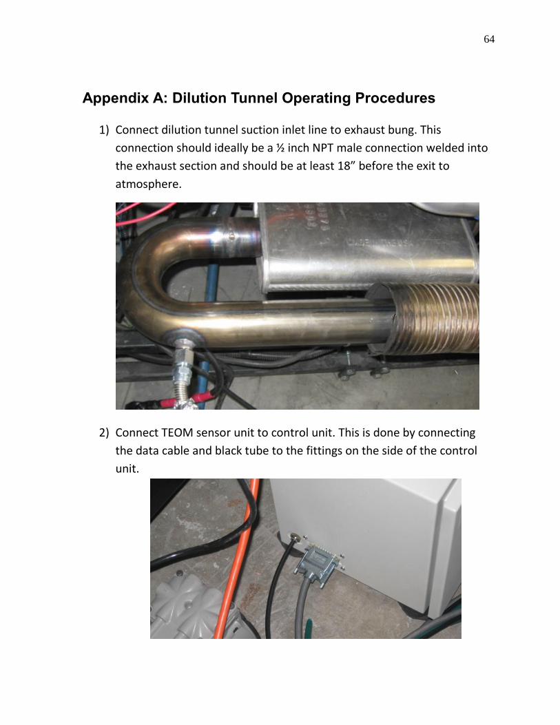
64

Appendix A: Dilution Tunnel Operating Procedures

1) Connect dilution tunnel suction inlet line to exhaust bung. This

connection should ideally be a ½ inch NPT male connection welded into

the exhaust section and should be at least 18” before the exit to

atmosphere.

2) Connect TEOM sensor unit to control unit. This is done by connecting

the data cable and black tube to the fittings on the side of the control

unit.

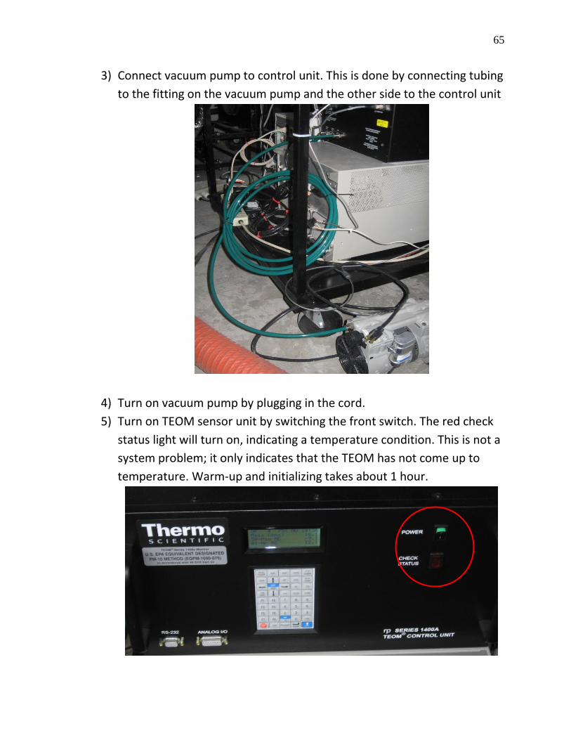
65

3) Connect vacuum pump to control unit. This is done by connecting tubing

to the fitting on the vacuum pump and the other side to the control unit

4) Turn on vacuum pump by plugging in the cord.

5) Turn on TEOM sensor unit by switching the front switch. The red check

status light will turn on, indicating a temperature condition. This is not a

system problem; it only indicates that the TEOM has not come up to

temperature. Warm-up and initializing takes about 1 hour.

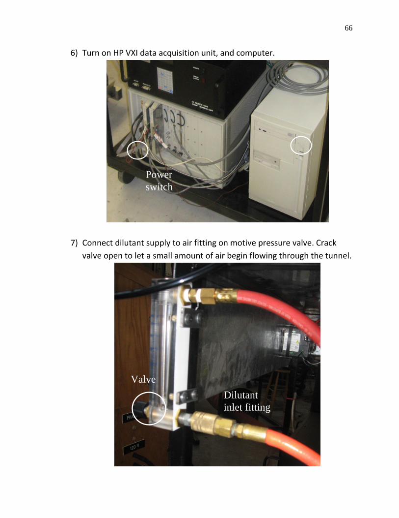
66

6) Turn on HP VXI data acquisition unit, and computer.

7) Connect dilutant supply to air fitting on motive pressure valve. Crack

valve open to let a small amount of air begin flowing through the tunnel.

Power

switch

Dilutant

inlet fitting

Valve

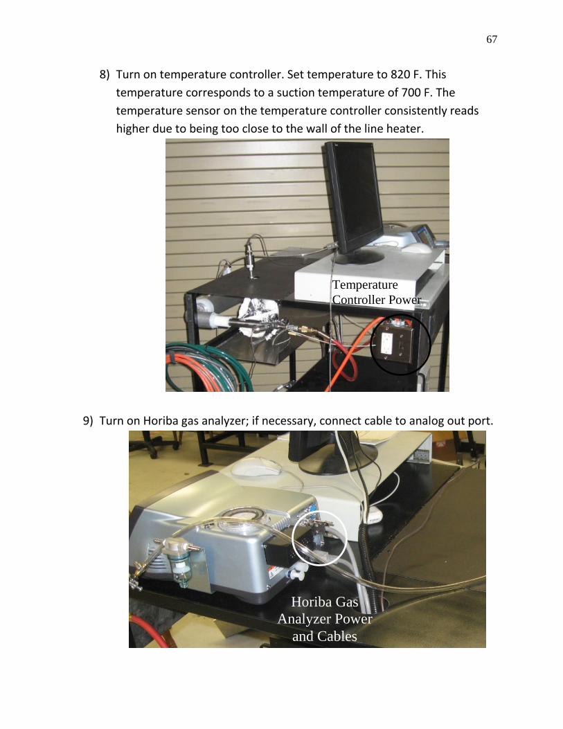
67

8) Turn on temperature controller. Set temperature to 820 F. This

temperature corresponds to a suction temperature of 700 F. The

temperature sensor on the temperature controller consistently reads

higher due to being too close to the wall of the line heater.

9) Turn on Horiba gas analyzer; if necessary, connect cable to analog out port.

Temperature

Controller Power

Horiba Gas

Analyzer Power

and Cables

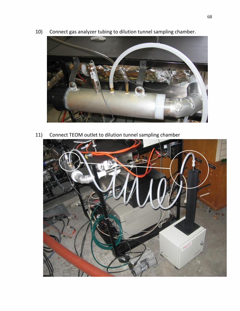
68

10) Connect gas analyzer tubing to dilution tunnel sampling chamber.

11) Connect TEOM outlet to dilution tunnel sampling chamber

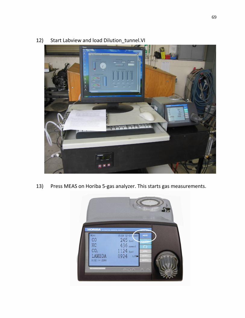
69

12) Start Labview and load Dilution_tunnel.VI

13) Press MEAS on Horiba 5-gas analyzer. This starts gas measurements.

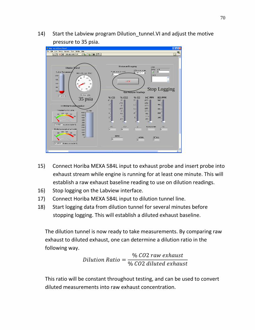
70

14) Start the Labview program Dilution_tunnel.VI and adjust the motive

pressure to 35 psia.

15) Connect Horiba MEXA 584L input to exhaust probe and insert probe into

exhaust stream while engine is running for at least one minute. This will

establish a raw exhaust baseline reading to use on dilution readings.

16) Stop logging on the Labview interface.

17) Connect Horiba MEXA 584L input to dilution tunnel line.

18) Start logging data from dilution tunnel for several minutes before

stopping logging. This will establish a diluted exhaust baseline.

The dilution tunnel is now ready to take measurements. By comparing raw

exhaust to diluted exhaust, one can determine a dilution ratio in the

following way.

𝐷𝑖𝑙𝑢𝑡𝑖𝑜𝑛 𝑅𝑎𝑡𝑖𝑜 =% 𝐶𝑂2 𝑟𝑎𝑤 𝑒𝑥ℎ𝑎𝑢𝑠𝑡

% 𝐶𝑂2 𝑑𝑖𝑙𝑢𝑡𝑒𝑑 𝑒𝑥ℎ𝑎𝑢𝑠𝑡

This ratio will be constant throughout testing, and can be used to convert

diluted measurements into raw exhaust concentration.

35 psia

Stop Logging

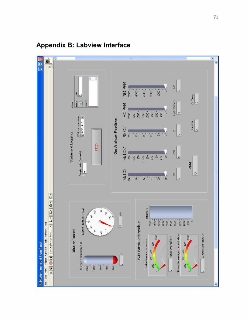
71

Appendix B: Labview Interface

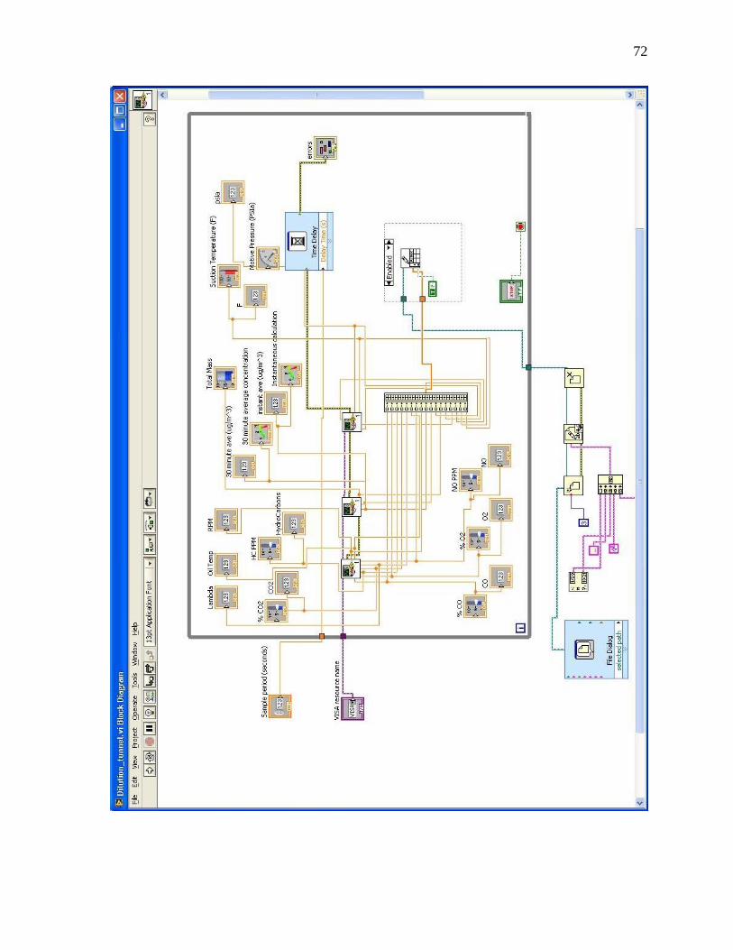
72

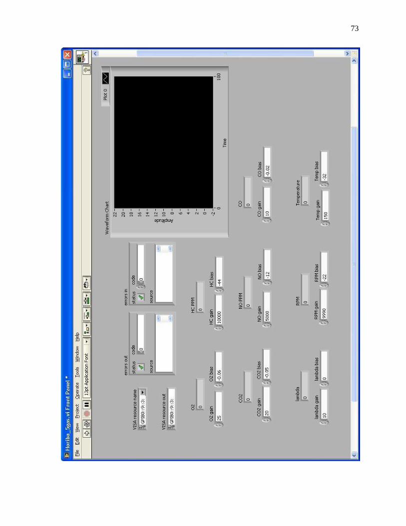
73

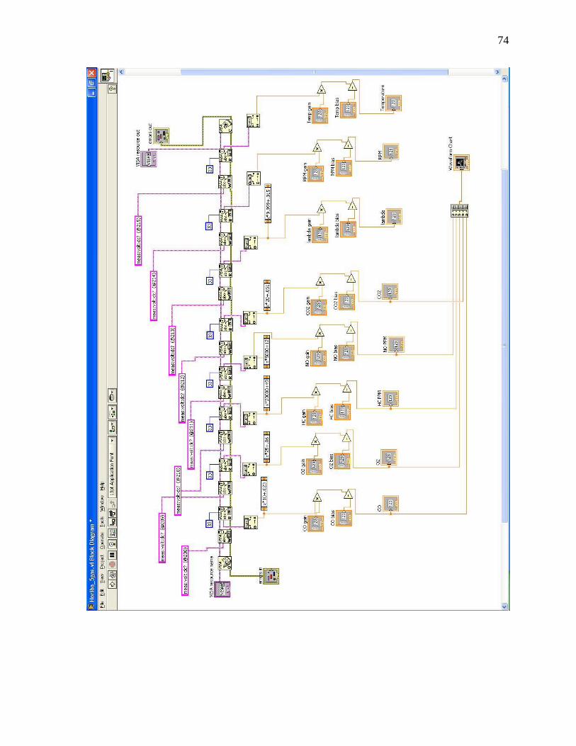
74

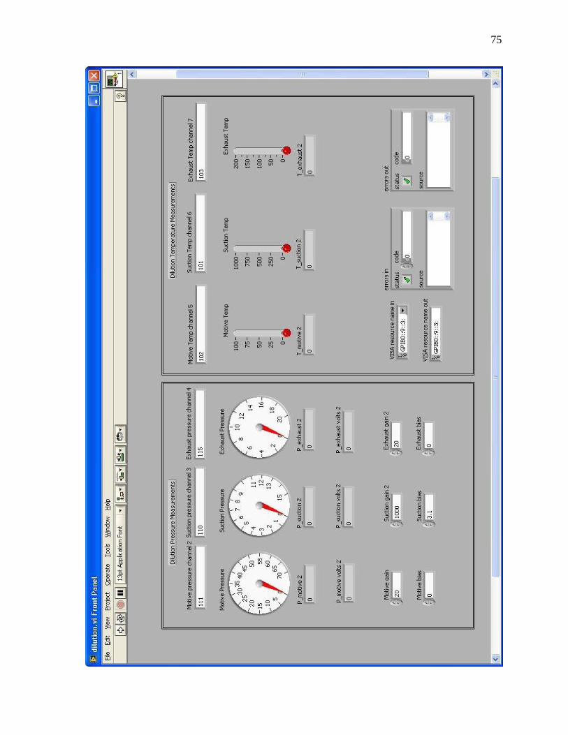
75

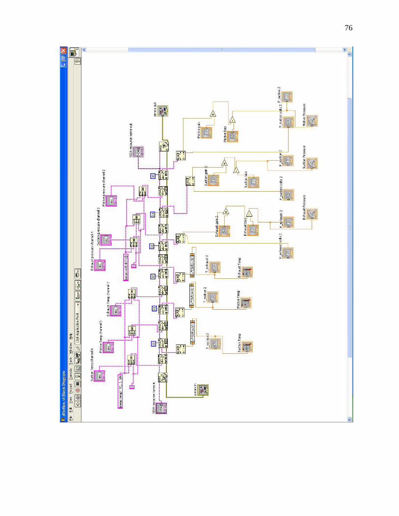
76

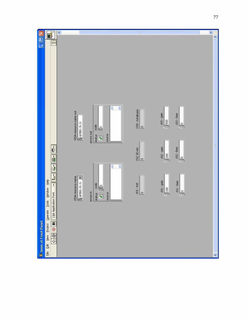
77

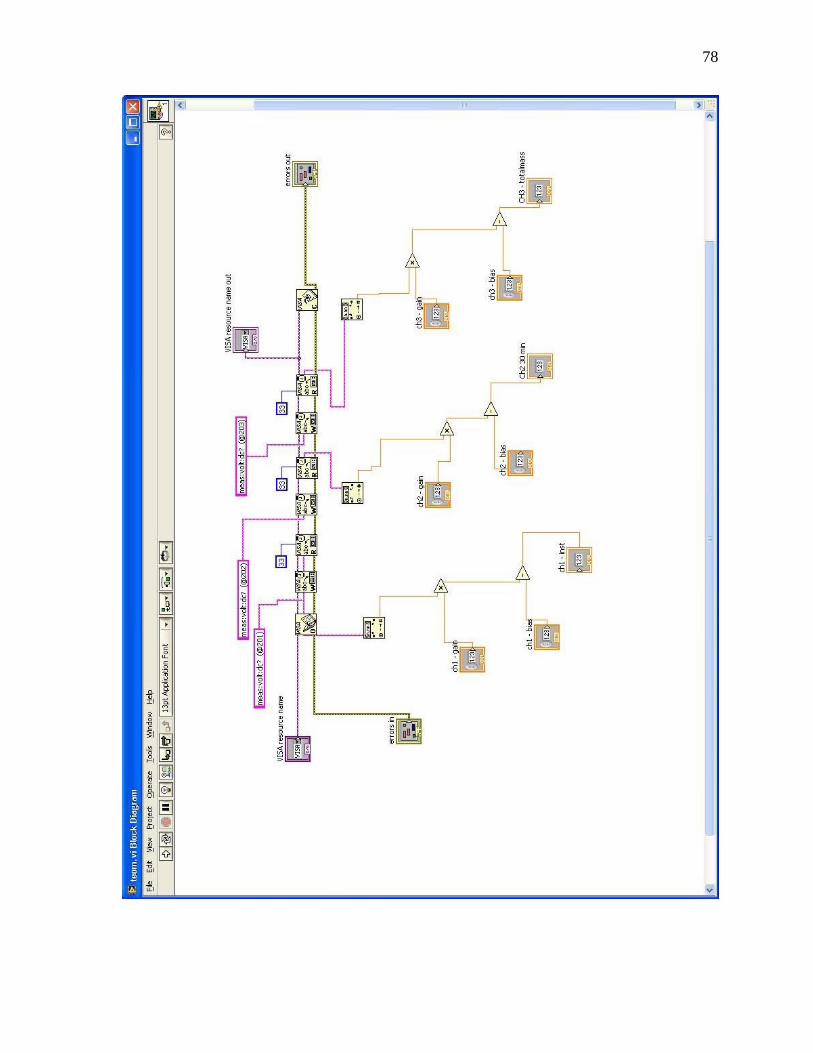
78

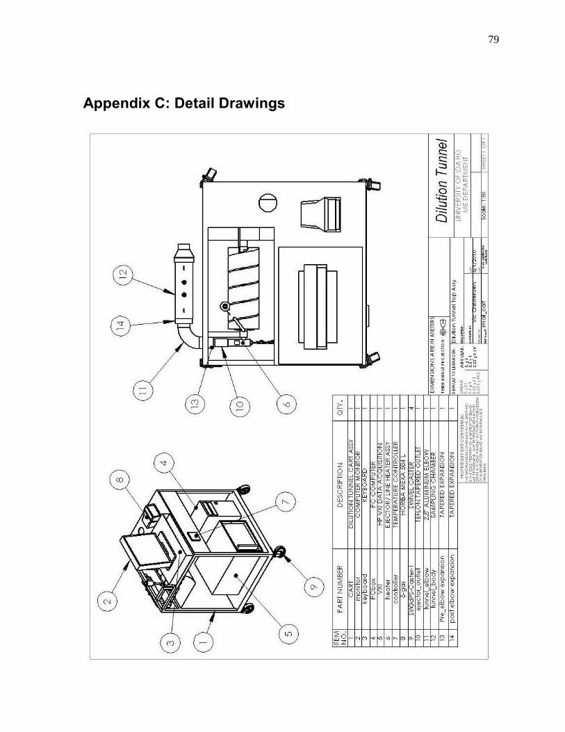
79

Appendix C: Detail Drawings

80

81

82

83

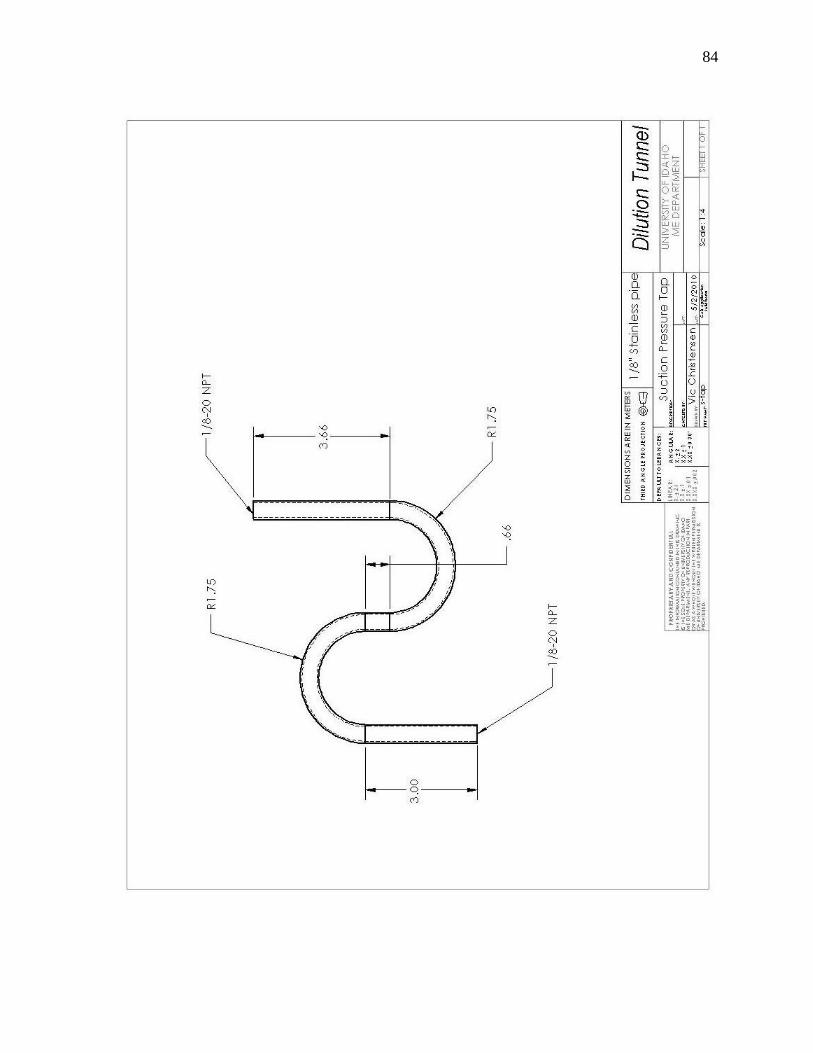
84

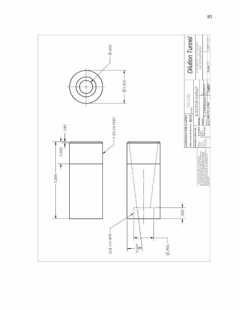
85

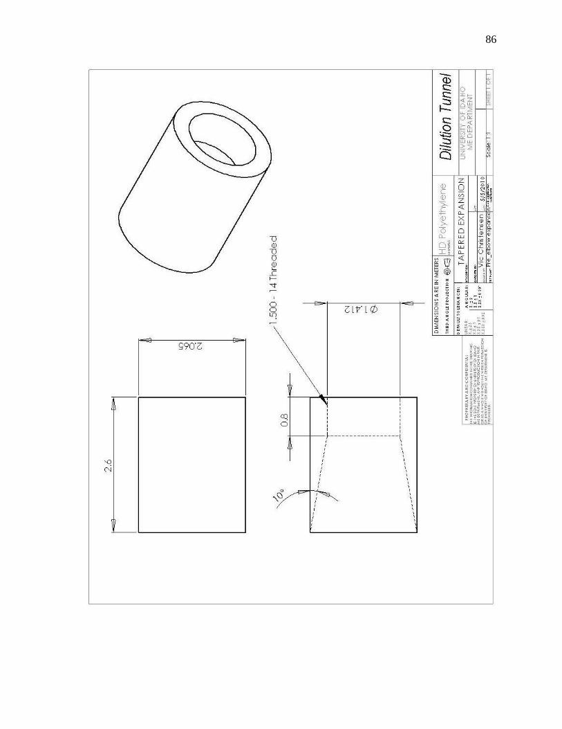
86

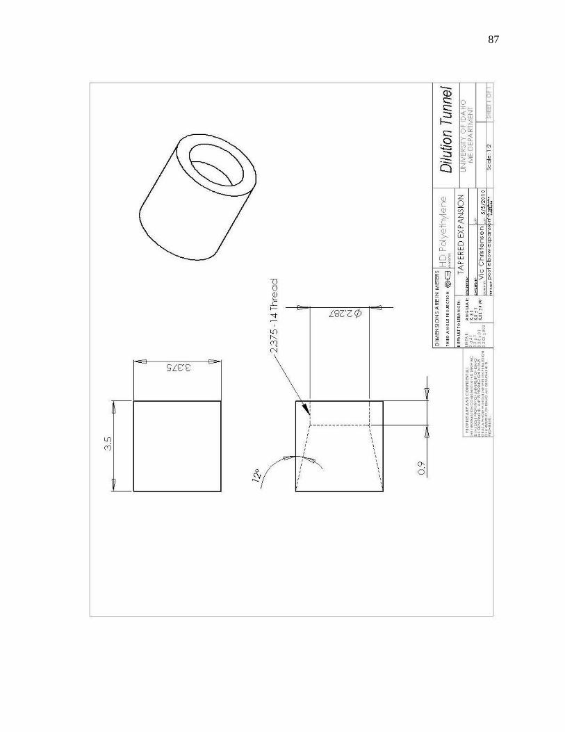
87

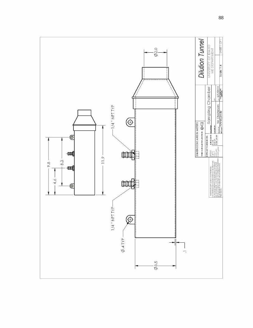
88

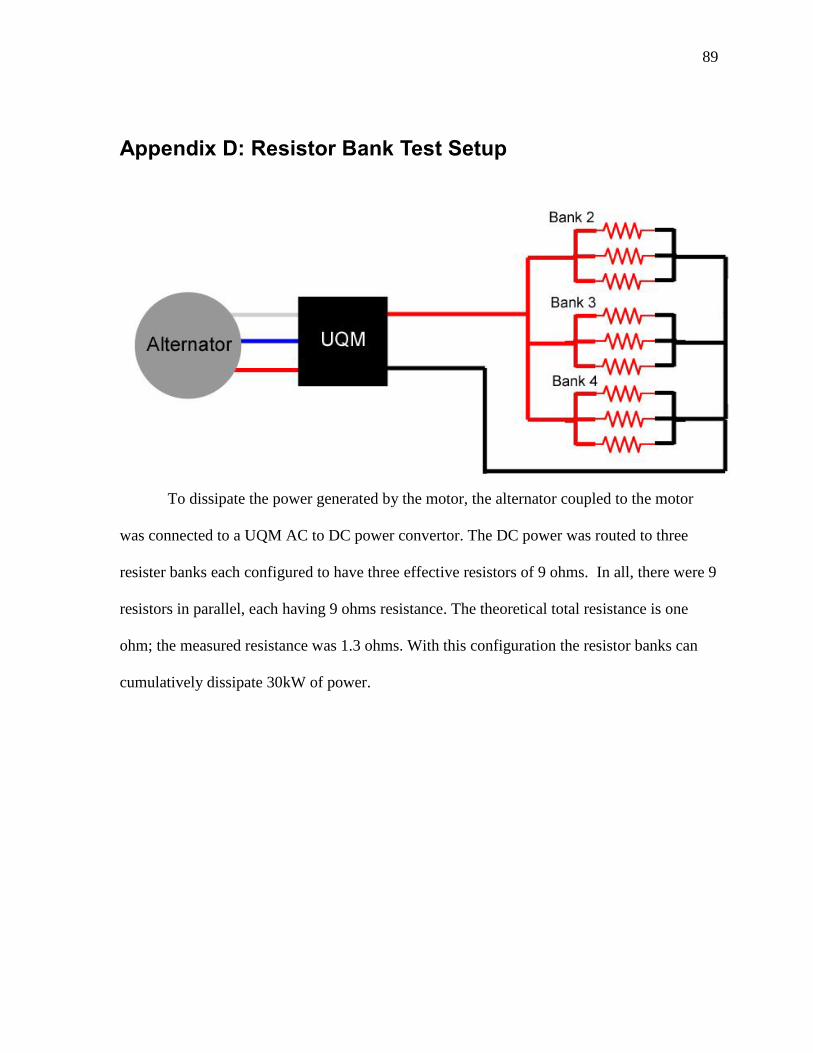
89

Appendix D: Resistor Bank Test Setup

To dissipate the power generated by the motor, the alternator coupled to the motor

was connected to a UQM AC to DC power convertor. The DC power was routed to three

resister banks each configured to have three effective resistors of 9 ohms. In all, there were 9

resistors in parallel, each having 9 ohms resistance. The theoretical total resistance is one

ohm; the measured resistance was 1.3 ohms. With this configuration the resistor banks can

cumulatively dissipate 30kW of power.

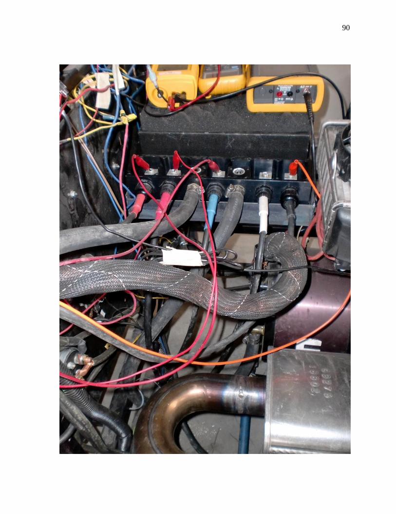
90

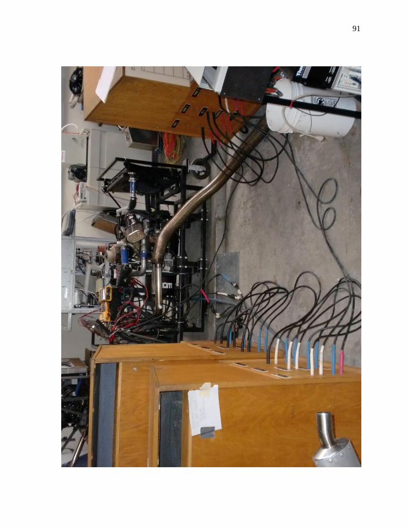
91

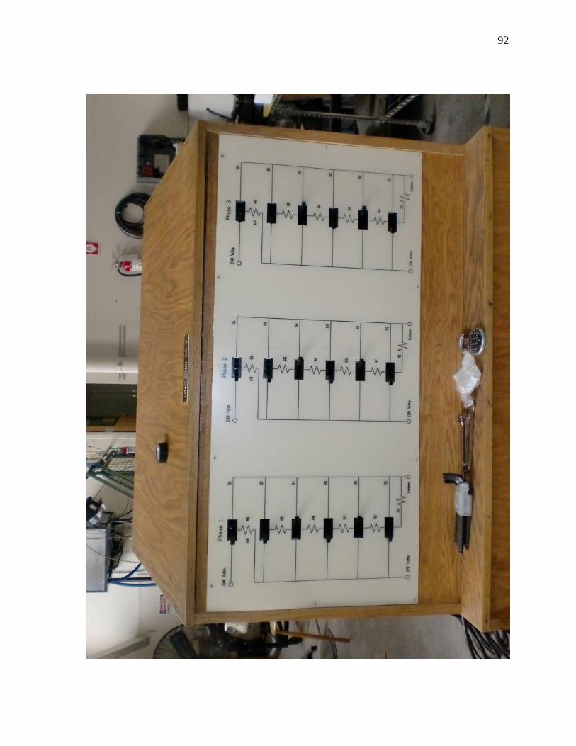
92

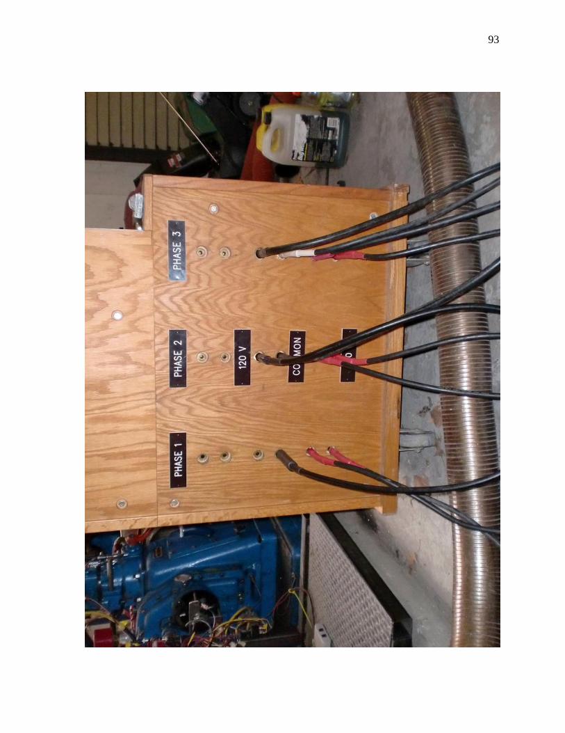
93

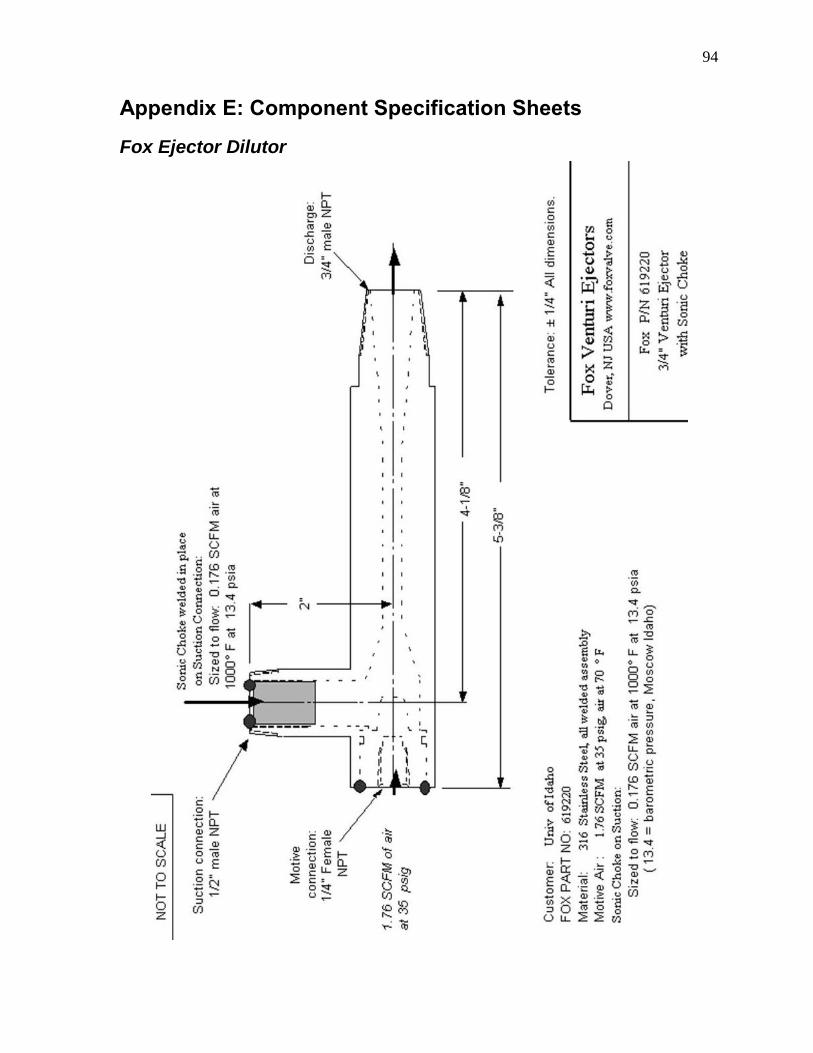
94

Appendix E: Component Specification Sheets

Fox Ejector Dilutor

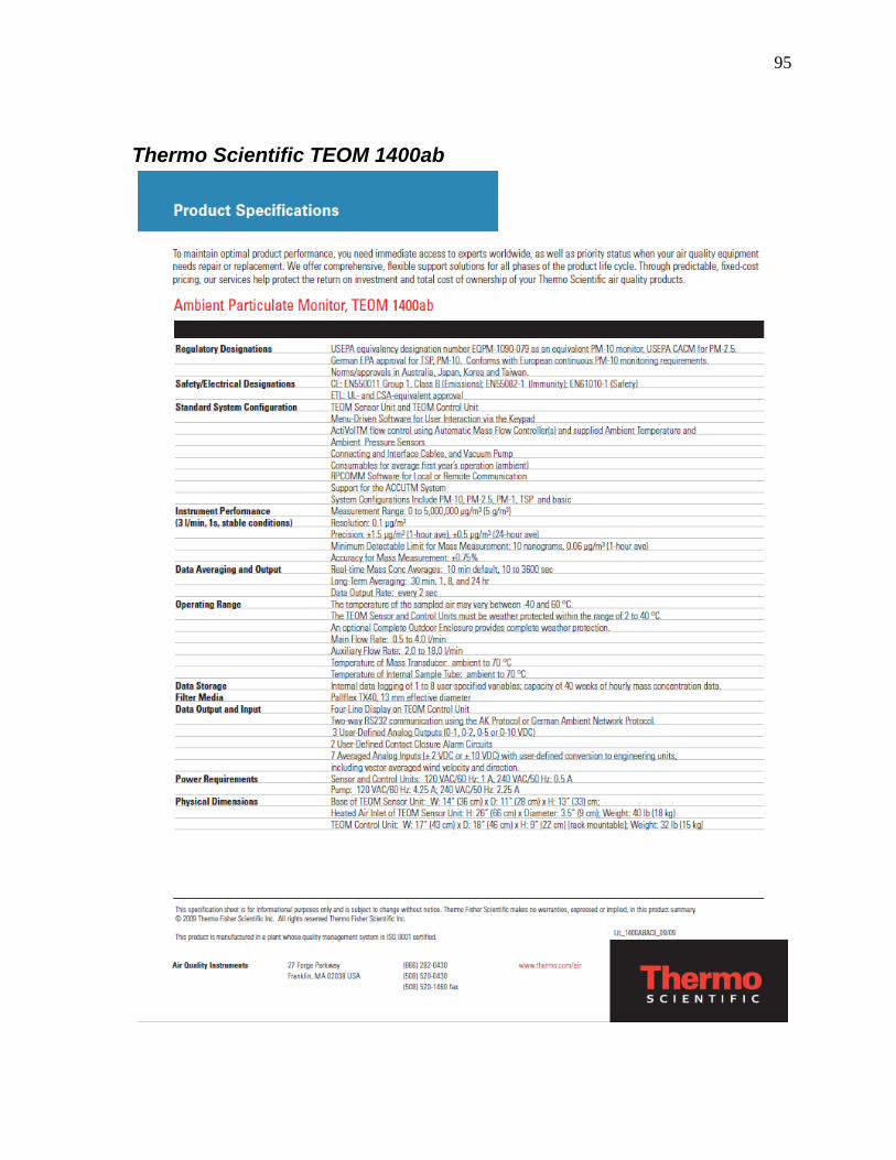
95

Thermo Scientific TEOM 1400ab

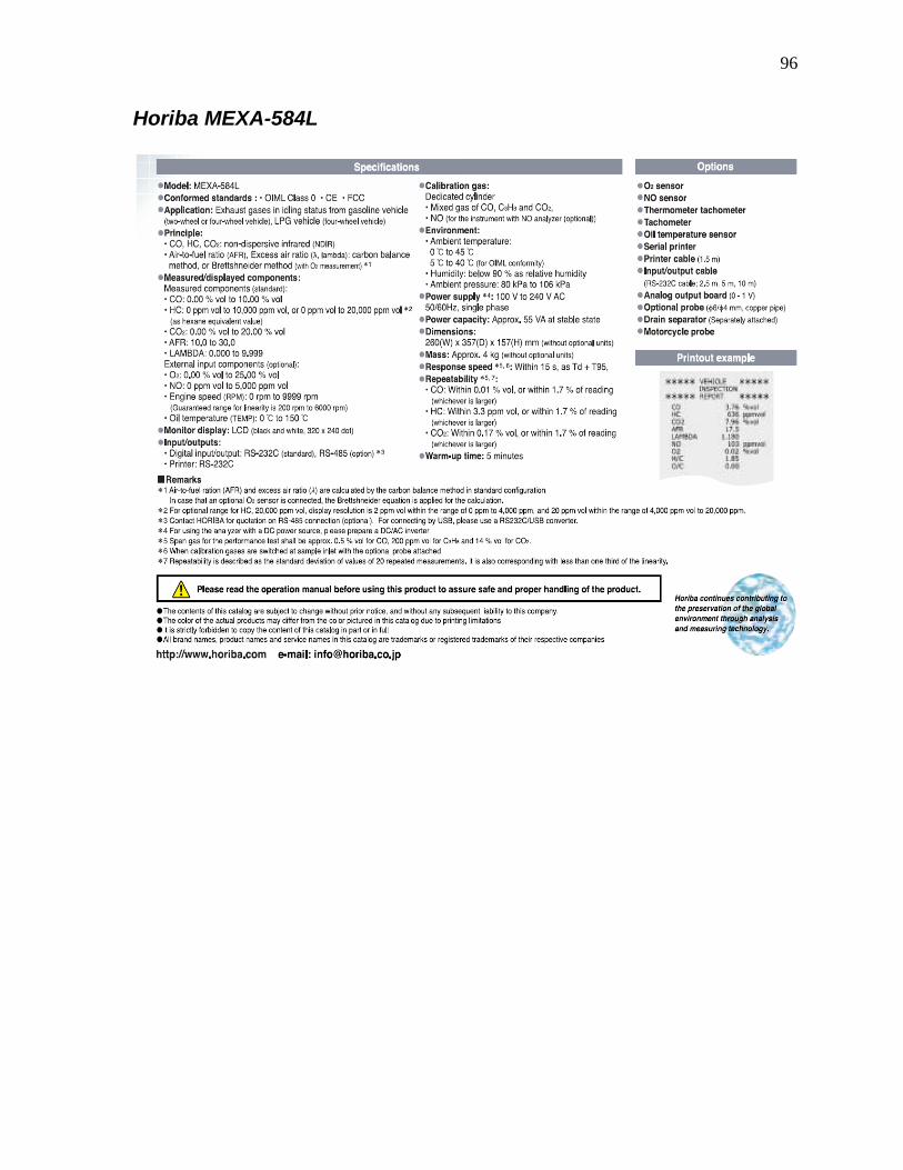
96

Horiba MEXA-584L

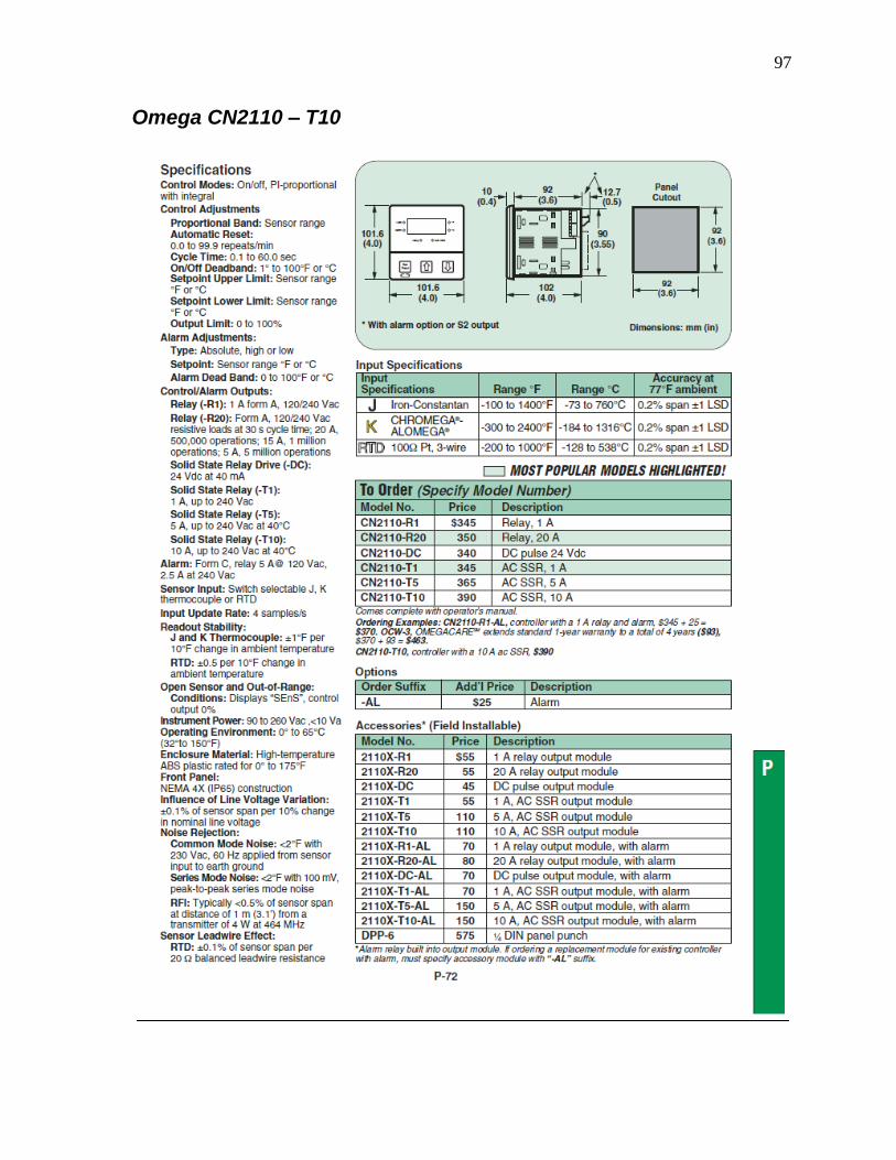
97

Omega CN2110 – T10