Embed Size (px)
Citation preview
Design-Basis Flood Estimation for Site Characterization at Nuclear Power Plants in the United States of America
Office of Nuclear Regulatory Research
NUREG/CR-7046 PNNL-20091

DISCLAIMER: This report was prepared as an account of work sponsored by an agency of the U.S. Government. Neither the U.S. Government nor any agency thereof, nor any employee, makes any warranty, expressed orimplied, or assumes any legal liability or responsibility for any third party’s use, or the results of such use, of anyinformation, apparatus, product, or process disclosed in this publication, or represents that its use by such thirdparty would not infringe privately owned rights.
AVAILABILITY OF REFERENCE MATERIALSIN NRC PUBLICATIONS
NRC Reference Material
As of November 1999, you may electronically accessNUREG-series publications and other NRC records atNRC’s Public Electronic Reading Room at http://www.nrc.gov/reading-rm.html. Publicly releasedrecords include, to name a few, NUREG-seriespublications; Federal Register notices; applicant,licensee, and vendor documents and correspondence;NRC correspondence and internal memoranda;bulletins and information notices; inspection andinvestigative reports; licensee event reports; andCommission papers and their attachments.
NRC publications in the NUREG series, NRCregulations, and Title 10, Energy, in the Code ofFederal Regulations may also be purchased from oneof these two sources.1. The Superintendent of Documents U.S. Government Printing Office Mail Stop SSOP Washington, DC 20402–0001 Internet: bookstore.gpo.gov Telephone: 202-512-1800 Fax: 202-512-22502. The National Technical Information Service Springfield, VA 22161–0002 www.ntis.gov 1–800–553–6847 or, locally, 703–605–6000
A single copy of each NRC draft report for comment isavailable free, to the extent of supply, upon writtenrequest as follows:Address: U.S. Nuclear Regulatory Commission Office of Administration Publications Branch Washington, DC 20555-0001E-mail: [email protected] Facsimile: 301–415–2289
Some publications in the NUREG series that are posted at NRC’s Web site addresshttp://www.nrc.gov/reading-rm/doc-collections/nuregs are updated periodically and may differ from the lastprinted version. Although references to material foundon a Web site bear the date the material was accessed,the material available on the date cited maysubsequently be removed from the site.
Non-NRC Reference Material
Documents available from public and special technicallibraries include all open literature items, such asbooks, journal articles, and transactions, FederalRegister notices, Federal and State legislation, andcongressional reports. Such documents as theses,dissertations, foreign reports and translations, andnon-NRC conference proceedings may be purchasedfrom their sponsoring organization.
Copies of industry codes and standards used in asubstantive manner in the NRC regulatory process aremaintained at—
The NRC Technical Library Two White Flint North11545 Rockville PikeRockville, MD 20852–2738
These standards are available in the library for reference use by the public. Codes and standards areusually copyrighted and may be purchased from theoriginating organization or, if they are AmericanNational Standards, from—
American National Standards Institute11 West 42nd StreetNew York, NY 10036–8002www.ansi.org 212–642–4900
Legally binding regulatory requirements are statedonly in laws; NRC regulations; licenses, includingtechnical specifications; or orders, not in NUREG-series publications. The views expressedin contractor-prepared publications in this series arenot necessarily those of the NRC.
The NUREG series comprises (1) technical andadministrative reports and books prepared by thestaff (NUREG–XXXX) or agency contractors(NUREG/CR–XXXX), (2) proceedings ofconferences (NUREG/CP–XXXX), (3) reportsresulting from international agreements(NUREG/IA–XXXX), (4) brochures(NUREG/BR–XXXX), and (5) compilations of legaldecisions and orders of the Commission and Atomicand Safety Licensing Boards and of Directors’decisions under Section 2.206 of NRC’s regulations(NUREG–0750).
Design-Basis Flood Estimation for Site Characterization at Nuclear Power Plants in the United States of America Manuscript Completed: December 2010 Date Published: November 2011 Prepared by Rajiv Prasad Lyle F. Hibler Andre M. Coleman Duane L. Ward Pacific Northwest National Laboratory P.O. Box 999 Richland, WA 99352 John D. Randall, NRC Project Manager Thomas J. Nicholson, NRC Technical Monitor NRC Job Code N6575 Office of Nuclear Regulatory Research
NUREG/CR-7046 PNNL-20091

iii
ABSTRACT
The purpose of this document is to describe approaches and methods for estimation of the design-basis flood at nuclear power plant sites. Chapter 1 defines the design-basis flood and lists the U.S. Nuclear Regulatory Commission’s (NRC) regulations that require estimation of the design-basis flood. For comparison, the design-basis flood estimation methods used by other Federal agencies are also described. A brief discussion of the recommendations of the International Atomic Energy Agency for estimation of the design-basis floods in its member States is also included.
Chapter 2 introduces the concept of hierarchical hazard assessment (HHA) and its application to estimation of the design-basis flood at nuclear power plant sites. The HHA consists of a series of progressively refined methods that increasingly use site-specific data to demonstrate whether the plant structures, systems, and components important to safety are adequately protected from the adverse effects of severe floods. The HHA method is illustrated by an example.
Chapter 3 introduces the concept of alternative conceptual models that are used to characterize the severe flooding scenarios at and near the site. The individual flood-causing hydrologic and hydrodynamic mechanisms are also described along with the potentially adverse effects they may cause at the site. A description of the HHA method as applied to several of these flooding mechanisms is provided. A brief discussion of combined events is also included.
Chapter 4 briefly describes two analytical approaches, the deterministic and the probabilistic, used in standard engineering practice for estimation of design-basis floods. The current NRC approach for estimation of design-basis floods uses the deterministic approach.
Chapter 5 describes the NRC’s quality assurance criteria for simulation models and provides a description of criteria used in selection of simulation models. A discussion of uncertainty in input data and model parameters is provided. A brief discussion of validation of model-derived estimates is also included. This chapter also provides a discussion of probabilistic approaches to estimation of flood hazard assessment and outlines the components of a formal Probabilistic Flood Hazard Assessment (PFHA) approach.
Chapter 5 also includes a brief summary of the findings of the fourth assessment report on climate change prepared by the Intergovernmental Panel on Climate Change. A brief note is made regarding incorporation of the effects of climate change in estimation of the design-basis floods at nuclear power plant sites. Some future directions for further refinement of design-basis flood estimation methods are also provided.
Chapter 6 provides a few specific recommendations for further research. Two of these are worth noting. Incorporation of more recent site-specific datasets to demonstrate the validity of estimated design-basis flood and available margins would provide additional assurance regarding safety. Development of a comprehensive PFHA methodology that leverages existing techniques in areas of hydrologic and hydraulic simulation, accounting for uncertainty in model inputs and parameters, and probabilistic flood frequency analysis can provide an extremely useful tool for risk-informed design-basis flood estimation at nuclear power plant sites.
The report also contains nine appendices. One of these appendices describes currently available hydrometeorological datasets and geographical information system techniques that are useful in data preprocessing and synthesis of model inputs. Seven of the other appendices describe the flood estimation techniques for various flood-causing mechanisms. The last appendix describes some limitations of the unit hydrograph approach frequently used in estimation of design-basis floods and recommends a method for adjusting unit hydrographs to make them more appropriate for estimation of extreme floods.

v
TABLE OF CONTENTS
Section Page
ABSTRACT .................................................................................................................................. iii LIST OF FIGURES ......................................................................................................................vii LIST OF TABLES .........................................................................................................................vii EXECUTIVE SUMMARY ..............................................................................................................ix
ACKNOWLEDGMENTS ............................................................................................................ xiii ACRONYMS AND ABBREVIATIONS ......................................................................................... xv
1 DESIGN-BASIS FLOOD ................................................................................................ 1-1
1.1 Definition of a Design-Basis Flood ................................................................................. 1-1
1.2 Design-Basis Flood Estimation Methods Adopted by Other Federal Agencies ............. 1-2
1.2.1 U.S. Army Corps of Engineers ....................................................................................... 1-3
1.2.2 Bureau of Reclamation ................................................................................................... 1-4
1.2.3 U.S. Department of Energy ............................................................................................ 1-4
1.3 Federal Energy Regulatory Commission ....................................................................... 1-5
1.4 Design-Basis Flood Estimation Guidelines of the International Atomic Energy Agency 1-6
2 THE HIERARCHICAL HAZARD ASSESSMENT APPROACH ...................................... 2-1
3 CAUSATIVE MECHANISMS FOR DESIGN-BASIS FLOODS ....................................... 3-1
3.1 Alternative Conceptual Models ...................................................................................... 3-1
3.2 Local Intense Precipitation ............................................................................................. 3-1
3.2.1 Flood Generated by Local Intense Precipitation and Its Effects..................................... 3-1
3.2.2 Hierarchical Hazard Assessment Applied to a Local Intense Precipitation-Generated Flood .............................................................................................................................. 3-2
3.3 Flooding in Rivers and Streams ..................................................................................... 3-3
3.3.1 Estimating the PMF and Its Effects ................................................................................ 3-3
3.3.2 Hierarchical Hazard Assessment Applied to PMF ......................................................... 3-4
3.4 Dam Breaches and Failures ........................................................................................... 3-5
3.4.1 Hierarchical Hazard Assessment Applied to Dam Breaches and Failures ..................... 3-5
3.5 Storm Surge ................................................................................................................... 3-6
3.5.1 Hierarchical Hazard Assessment Applied to PMSS ....................................................... 3-8
3.6 Seiche ............................................................................................................................ 3-9
3.7 Ice-Induced Flooding ...................................................................................................... 3-9
3.8 Flooding Resulting from Channel Migration or Diversion ............................................. 3-10
3.9 Combined-Effects Flood ............................................................................................... 3-10
4 APPROACHES .............................................................................................................. 4-1
4.1 Deterministic Analyses ................................................................................................... 4-1
4.2 Probabilistic Analyses .................................................................................................... 4-3
5 DESIGN-BASIS FLOOD HAZARD ESTIMATION METHODS ....................................... 5-1
5.1 Alternative Conceptual Models ...................................................................................... 5-1
vi
5.2 Quality Assurance Criteria for Simulation Models .......................................................... 5-3
5.3 Selecting Simulation Models to Use ............................................................................... 5-3
5.4 Accounting for Uncertainty in Input and Model Parameters for Estimation of Design-Basis Flood Hazards ...................................................................................................... 5-5
5.5 Validation ....................................................................................................................... 5-6
5.6 Reconciling Deterministic and Probabilistic Notions in the Context of Design-Basis Flood Estimation ............................................................................................................ 5-6
5.7 Effects of Climate Variability on Design-Basis Flood Estimation.................................... 5-9
6 FUTURE DIRECTIONS ................................................................................................. 6-1
7 REFERENCES ............................................................................................................... 7-1
8 GLOSSARY ................................................................................................................... 8-1
APPENDIX A HYDROLOGICAL DATA SOURCES .................................................................. A-1
APPENDIX B FLOODING FROM LOCAL INTENSE PRECIPITATION: A CASE STUDY ....... B-1
APPENDIX C DATA PREPARATION AND WATERSHED MODELING SETUP ..................... C-1
APPENDIX D FLOODING FROM DAM BREACHES AND FAILURES: A CASE STUDY ....... D-1
APPENDIX E FLOODING FROM STORM SURGES: A CASE STUDY ................................... E-1
APPENDIX F FLOODING FROM A SEICHE: A CASE STUDY ............................................... F-1
APPENDIX G FLOODING FROM ICE-INDUCED EVENTS: A CASE STUDY ....................... G-1
APPENDIX H COMBINED-EFFECT FLOODS ......................................................................... H-1
APPENDIX I UNIT HYDROGRAPHS AND NONLINEAR HYDROLOGIC RESPONSE ............. I-1

vii
LIST OF FIGURES
Figure Page
2-1. Flowchart Demonstrating the HHA Applied to Flood Hazards from a PMF Event ......... 2-3
5-1. A Hypothetical Nuclear Power Plant Site Location with Respect to a Creek, a River, Two Bays, and an Ocean (map elements are not to scale) ................................. 5-2
LIST OF TABLES
Table Page
3-1. Types of Tropical Storms and the Saffir-Simpson Scale Describing the Categories of Hurricanes… .................................................................................................................. 3-7
.

ix
EXECUTIVE SUMMARY
The last revision of Regulatory Guide 1.59 was published by the U.S. Nuclear Regulatory Commission (NRC) in 1977. Since that time, flood estimation techniques have significantly advanced. The availability of more accurate datasets and advent of new analysis methodologies such as geographical information systems has facilitated rapid processing of large, spatially distributed datasets in the estimation of input for newer classes of hydrologic, hydraulic, and hydrodynamic models. This report attempts to collect relevant information that can be used in the estimation of design-basis floods at nuclear power plant sites.
The experience gained by the staff at Pacific Northwest National Laboratory over the last few years while assisting the NRC staff in the review of Early Site Permits and Combined License Applications has resulted in the development of new and efficient techniques that are expected to provide substantial gains in the accuracy and reliability of the estimates of design-basis floods.
The NRC regulations require a safety analysis to demonstrate that structures, systems, and components (SSCs) important to safety of a nuclear power plant are adequately protected from the adverse effects of flooding. This report describes a new approach, the hierarchical hazard assessment (HHA) approach, tailored to the estimation of design-basis flood hazard metrics at a given site. The HHA is a stepwise, progressively refined series of analyses that is aimed at demonstrating that the SSCs important to safety are adequately protected from the adverse effects of severe floods expected at the site.
At the start of the estimation of design-basis flood hazards, it is very useful to list clearly all plausible flooding mechanisms that are capable of generating a severe flood at the site. It is also readily recognized that several scenarios of a particular flooding mechanism can affect the site; for example, precipitation-generated floods may occur in a river adjacent to the site as well as in a tributary that flows past the site. Multiple scenarios resulting from alternative conceptual models of flooding from other mechanisms should also be investigated.
It may be possible to determine that some alternative conceptual models of flooding are demonstrably less conservative than others and therefore more detailed analyses of those scenarios may not be necessary. At the same time, enumeration of all plausible alternative conceptual models provides additional assurance that the complete range of possible scenarios at the site is adequately accounted for.
This report briefly discusses the probabilistic approaches to estimation of design-basis floods. However, the deterministic approach currently in use is recommended for the near future because of two reasons: the lack of an overall framework that fully implements a Probabilistic Flood Hazard Assessment (PFHA) and to ensure consistency with current practices.
Nevertheless, several advances can be recommended at this time. Availability of large, spatially distributed datasets and tools for rapid processing of these datasets provides an opportunity to refine the representation of modeling elements in the drainage basin and to parameterize more accurately the models currently used in practice. The availability of more than 30 years of additional data since the last revision of Regulatory Guide 1.59 also provides a longer and more robust validation dataset. Advances in computing speeds and availability of specialized software also reduce the time required for analysis, allowing the examination of multiple scenarios and thereby helping to reduce uncertainty in estimates of design-basis flood hazards.

x
The report contains nine appendices, seven of which present examples of flood estimation from various mechanisms. Only flood-simulation models currently accepted and widely used have been employed in the development of these examples. However, these examples should not be construed to be the only or even the most appropriate approach for estimation of design-basis flood hazard metrics at a particular site. Often, site-specific conditions greatly influence not only parameter choices but also the selection of the simulation models themselves. Some of these issues are discussed in Chapter 5 of this report.
Recently, debate has focused on the projected climate change in the latter parts of the twenty-first century and what these projections mean to the estimation of design-basis flood hazards at sites where nuclear power plants may be expected to be in operation during the same period. Chapter 5 summarizes the findings of the Intergovernmental Panel on Climate Change fourth assessment report of 2007. Several hydroclimatic changes are projected for the United States. However, the complete effect of these projected changes on flood-causing mechanisms has not been investigated in detail at various spatial scales needed for site characterization at nuclear power plants. For example, surface temperature and precipitation are both projected to increase in eastern North America. The North Atlantic is also projected to be warmer. The effects of these changes on synoptic and monsoon patterns that govern precipitation have not been studied yet. It is possible that these changes would result in a different climate where current estimates of extreme precipitation may not hold true. In absence of any definitive studies, this report recommends that the projected changes be incorporated in the estimation of design-basis flood hazard as sensitivity studies. The results of these sensitivity studies should be used to determine and clearly report the margin available between the selected design basis and the (uncertain) site characteristic related to each flood hazard metric.
Probabilistic flood assessment has the benefit of clearly articulating the exceedance frequency of a selected design basis. Therefore, it facilitates a risk-informed approach to decision-making. Several components of PFHA already exist and have matured over the past few decades. However, the near-future need is to develop an overall framework where these techniques can be integrated into a comprehensive PFHA tool.

xi
PAPERWORK REDUCTION ACT STATEMENT
This NUREG does not contain information collection requirements and, therefore, is not subject to the requirements of the Paperwork Reduction Act of 1995 (44 USC 3501, et seq.).
PUBLIC PROTECTION NOTIFICATION
The NRC may not conduct or sponsor, and a person is not required to respond to, a request for information or an information collection requirement unless the requesting document displays a currently valid Office of Management and Budget control number.


xiii
ACKNOWLEDGMENTS
The authors sincerely acknowledge technical discussions, guidance, and suggestions provided by Mr. Lance Vail, Dr. Mark Wigmosta, and Dr. Michael Fayer of PNNL. Technical comments provided by Mr. Goutam Bagchi, Dr. Hosung Ahn, Dr. Henry Jones, Dr. Nebiyu Tiruneh, Dr. Christopher Cook, Dr. Ann Kammerer, Dr. Fernando Ferrante, Mr. Thomas Nicholson, Ms. Melanie Galloway, Dr. John Randall, and Dr. Joseph Giacinto, all of NRC; Dr. John England of the U.S. Bureau of Reclamation, and Dr. Donald Resio of the U.S. Army Corps of Engineers helped improve this report.
Financial support from the Office of Nuclear Regulatory Research of the NRC is gratefully acknowledged. Preparation of this report would have been impossible without the continued guidance and support of Dr. John Randall, the NRC Project Manager, and Mr. Thomas Nicholson, the NRC Technical Monitor.
Project management support from Ms. Janie Vickerman and Ms. Julie Hughes that kept this project sustained during difficult periods, is also acknowledged.
Excellent editorial support from Mr. Cary Counts, Ms. Susan Ennor, Ms. Jennifer Blake, and Ms. Meghan Spanner made this report possible.


xv
ACRONYMS AND ABBREVIATIONS
ºC degree(s) Celsius (or Centigrade)
ºF degree(s) Fahrenheit
ac acre(s)
ACRS Advisory Committee on Reactor Safeguards
ADCIRC Advanced Circulation
ANS American Nuclear Society
ANSI American National Standards Institute
CFR Code of Federal Regulations
cfs cubic (foot)feet per second
D-A-D depth-area-duration (curves)
DEM Digital Elevation Model
DHSVM Distributed Hydrology Soil-Vegetation Model
DOE U.S. Department of Energy
EHW envelop of high water
EM Engineer Manual
ER Engineer Regulation
ESP Early Site Permit
ESRI Environmental Systems Research Institute
FEMA Federal Emergency Management Agency
FERC Federal Energy Regulatory Commission
FSAR Final Safety Analysis Report
FTP file transfer protocol
GDC General Design Criteria
GIS Geographic Information System
HEC-HMS Hydrologic Engineering Center Hydrologic Modeling System
HEC-RAS Hydrologic Engineering Center River Analysis System

xvi
HHA hierarchical hazard assessment
HMR Hydrometeorological Report
hr hour(s)
HUC Hydrologic Unit Code
IAEA International Atomic Energy Agency
IACWD Interagency Advisory Committee on Water Data
in. inch
IPCC Intergovernmental Panel on Climate Change
LULC Land Use/Land Cover
km kilometer(s)
km2 square kilometer(s)
kPa kilopascal(s)
kt knot(s)
m meter(s)
mi2 square mile(s)
mb millibar
MEOW maximum envelope of water
mi mile(s)
min minute(s)
mm millimeter(s)
MOM maximum of the MEOWs
MRLC Multi-Resolution Land Characteristics Consortium
MSL mean sea level
NCDC National Climatic Data Center
NED National Elevation Dataset
NHD National Hydrography Dataset
NLCD National Land Cover Database
xvii
NOAA National Oceanic and Atmospheric Administration
NRC U.S. Nuclear Regulatory Commission
NRCS Natural Resources Conservation Service
NWS National Weather Service
OBE operating basis earthquake
PC performance category
PDF probability density function
PFHA Probabilistic Flood Hazard Assessment
PMF probable maximum flood
PMH probable maximum hurricane
PMP probable maximum precipitation
PMS probable maximum seiche
PMSS probable maximum storm surge
PMT probable maximum tsunami
PMWS probable maximum windstorm
PRA Probabilistic Risk Assessment
SCS Soil Conservation Service
SLOSH Sea, Lake, and Overland Surges from Hurricanes
SRTM Shuttle Radar Topographic Mission
SSCs structures, systems, and components
SSE safe shutdown earthquake
UH unit hydrograph
URL uniform resource locator
USACE U.S. Army Corps of Engineers
USGS United States Geological Survey
WMO World Meteorological Organization
WMS Watershed Modeling System

xviii

1-1
1 DESIGN-BASIS FLOOD
Nuclear power plants need to be protected from the adverse effects of flooding. To assist in determining the potential for adverse flooding effects, the U.S. Nuclear Regulatory Commission (NRC) provides guidance for estimating design-basis floods in Regulatory Guide 1.59 (NRC 1977).
1.1 Definition of a Design-Basis Flood
A design-basis flood is a flood caused by one or an appropriate combination of several hydrometeorological, geoseimic, or structural-failure phenomena, which results in the most severe hazards to structures, systems, and components (SSCs) important to the safety of a nuclear power plant.
Title 10 of the U.S. Code of Federal Regulations (CFR) 52.79(a)(1)(iii) states that a Final Safety-Analysis Report, which is part of the Combined Operating License application process for nuclear power plants, must address:
The seismic, meteorological, hydrologic, and geologic characteristics of the proposed site with appropriate consideration of the most severe of the natural phenomena that have been historically reported for the site and surrounding area and with sufficient margin for the limited accuracy, quantity, and time in which the historical data have been accumulated.
10 CFR 52.17(a)(1)(vi) includes a similar statement for Early Site Permit applications.
10 CFR 52.79(a)(4)(i) states that the minimum design requirements for the principal design criteria are established by 10 CFR Part 50, Appendix A, General Design Criteria for Nuclear Power Plants.
General Design Criterion 2 (GDC 2), Design bases for protection against natural phenomena, in Appendix A to 10 CFR Part 50, Domestic Licensing of Production and Utilization Facilities, states:
Structures, systems, and components important to safety shall be designed to withstand the effects of natural phenomena such as earthquakes, tornadoes, hurricanes, floods, tsunami, and seiches without loss of capability to perform their safety functions. The design bases for these structures, systems, and components shall reflect: (1) appropriate consideration of the most severe of the natural phenomena that have been historically reported for the site and surrounding area, with sufficient margin for the limited accuracy, quantity, and period of time in which the historical data have been accumulated, (2) appropriate combinations of the effects of normal and accident conditions with the effects of the natural phenomena, and (3) the importance of the safety functions to be performed. [Emphases in bold added by the authors.]
The requirements imposed by GDC 2 for determining a design-basis flood are (1) consideration of the most severe historical event with sufficient margin, (2) consideration of combinations of ambient conditions with flood-inducing natural phenomena, and (3) consideration of the importance of safety functions affected by flooding. GDC 2 also requires that SSCs important to safety must be able to perform their safety functions without loss of capability during a design-basis flood.
1-2
GDC 44, Cooling water, requires an ultimate heat sink to transfer heat from SSCs important to safety. The ultimate heat sink must remain functional under normal and accident conditions, including the design-basis flood.
10 CFR 100.20 requires nuclear power plant site evaluation to include meteorological, hydrological, seismic, and geologic characteristics that may affect the acceptability of a site for a stationary power reactor. 10 CFR 100.20 also requires evaluation of the nature and proximity of man-related hazards such as dams.
In the past, NRC adopted the concept of a “probable maximum event,” for estimating design bases. The probable maximum event, which is determined by accounting for the physical limits of the natural phenomenon, is the event that is considered to be the most severe reasonably possible at the location of interest and is thought to exceed the severity of all historically observed events. For example, a probable maximum flood (PMF) is the hypothetical flood generated in the drainage area by a probable maximum precipitation (PMP) event. The probable maximum storm surge (PMSS) is generated by the probable maximum hurricane (PMH) or the probable maximum windstorm (PMWS). These events are defined by the American National Standards Institute (ANSI) and American Nuclear Society (ANS) in ANSI/ANS-2.8-1992 (ANS 1992). Similar concepts exist for a probable maximum tsunami (PMT), which is not covered in this report. González et al. (2007) and Prasad (2009) discussed PMT hazards at nuclear power plant sites in the United States. The PMP is assumed to be a theoretical maximum and its estimation uses no associated probability distribution. In standard practice, estimating the PMF from the PMP involves some subjectivity and also uses no probabilistic basis.
More recently, probabilistic methods have also gained acceptance for determining design-basis events. The advantage of probabilistic methods is that an estimate of the probability-of-exceedance of the selected design basis can be made. This capability enables clear articulation of the level of risk that an SSC important to safety encounters during its operation. The emphasis, therefore, is not on determining the worst-case scenario as a basis for design, but to state the level of risk a chosen design would face.
1.2 Design-Basis Flood Estimation Methods Adopted by Other Federal Agencies
This section briefly describes the methods adopted by Federal agencies other than NRC for determining a design-basis flood. The U.S. Army Corps of Engineers (USACE), the Bureau of Reclamation (Reclamation), and the Federal Energy Regulatory Commission (FERC) estimate design-basis floods when designing and conducting safety assessments of flood-control structures, dams, water-supply infrastructure, and levees. The U.S. Department of Energy (DOE) estimates design-basis floods to help ensure the safety of SSCs at its facilities, and the Federal Emergency Management Agency (FEMA) determines design-basis floods so it can plan for emergency actions following a severe flooding event.
The methods recommended by USACE, Reclamation, DOE, and FERC for estimating design-basis floods are described in the following sections.
1-3
1.2.1 U.S. Army Corps of Engineers
USACE publishes a series of Engineer Regulations (ERs) and Engineer Manuals (EMs) (USACE 2009). The most relevant of these publications for estimating design-basis floods are as follows:
• EM 1110-2-1420 (Hydrologic Engineering Requirements for Reservoirs)
• EM 1110-2-1417 (Flood-Runoff Analysis)
• EM 1110-2-1406 (Runoff from Snowmelt)
• EM 1110-2-1411 (Standard Project Flood Determinations)
• EM 1110-2-1416 (River Hydraulics)
• EM 1110-2-1100 (Coastal Engineering Manual)
• EM 1110-2-1612 (Ice Engineering)
• ER 1110-8-2(FR) (Inflow Design Flood for Dams and Reservoirs)
• EM 1110-2-1603 (Hydraulic Design of Spillways)
• EM 1110-2-1605 (Hydraulic Design of Navigation Dams)
• EM 1110-2-3600 (Management of Water Control Systems)
• EC 1165-2-210 (Water Resources Policies and Authorities – Water Supply Storage and Risk Reduction Measures for Dam Safety).
USACE regulations currently state that dams for which failures may result in potential loss of human life must be designed safely to pass a flood inflow into the reservoir estimated from the PMP (USACE 1991). However, USACE is now using Probabilistic Risk Assessment (PRA) and risk analysis to assess the design adequacy and potential failure of dams and levees (USACE 2010). Hydrologic hazard estimates, which include flood probabilities up to the maximum event, are used as inputs to risk analysis. Extreme flood probability methods currently used by USACE are described by USACE (2008a) and summarized by Brunner and Gee (2009).
USACE typically uses generalized rainfall criteria from National Weather Service (NWS) Hydrometeorological Reports (HMRs) (e.g., Schreiner and Riedel 1978). However, in drainage basins where unusual conditions exist or where generalized criteria may not provide refined estimates of rainfall, special hydrometeorological studies may be performed.
USACE (1991, 1997) transforms rainfall to runoff using unit hydrographs and loss rates that are favorable for rapid watershed response. The peak discharges of unit hydrographs derived from observed flood events that are smaller than the PMF should be increased 20 to 50 percent. The water-surface elevation in a reservoir prior to the arrival of a PMF is assumed to be at the full pool level. USACE also considers an antecedent precipitation event prior to the arrival of the PMP event. USACE (1994) describes the process of using unit hydrographs including several synthetic hydrographs, but cautions that unit hydrographs intended for estimating large flood events such as the PMF should be derived from large historical flood events. It suggests that in certain cases, it is appropriate to modify the unit hydrograph to account for the shorter travel time expected for larger floods.
A portion of precipitation falling on the drainage basin does not contribute to direct runoff because of interception that is eventually evaporated from canopies, depression storage that eventually infiltrates, and evapotranspiration. The rate of precipitation loss during a PMF event
1-4
should be the most severe that is reasonable for the storm magnitude (USACE 1994). Loss rates observed or estimated from large historical flood events may be used if the hydrometeorological condition prevailing during these storms can be shown to represent severe conditions. USACE (1994) recommends that no losses be considered when the ground may be frozen at the start of the flood event. A similar argument may also be made for saturated soil conditions.
1.2.2 Bureau of Reclamation
Reclamation oversees, manages, and maintains over 350 large dams, reservoirs, and appurtenant facilities in the western United States as part of its responsibility to develop and conserve the nation’s water resources. The Reclamation Dam Safety Program is responsible for overseeing the safety assessments and potential modifications of existing dams, and for new dams. Reclamation uses risk analysis to prioritize financial resources on new and existing dams within Reclamation's inventory (Reclamation 2003). Reclamation's Public Protection Guidelines provide two risk criteria for assessing the safety of dams: potential loss of life and annual failure probability (Reclamation 2003). Reclamation's Best Practices in Dam Safety Risk Analysis (Reclamation 2010) describes in detail the technical methods for dam safety assessments that are used by Reclamation staff to assess the loads, structural response, consequences, and risk.
To assess a particular existing or new structure, Reclamation estimates the full probability distribution of hazards such as floods or earthquakes. Reclamation uses a suite of methods to estimate hydrologic hazard curves, which portray peak flows and volumes for a range of annual exceedance probabilities (Swain et al. 2006). Reclamation's policy is to use the PMF, as determined by the PMP, as the physical upper limit for hydrologic hazard curves (Reclamation 2002).
Reclamation has published a set of three design manuals for design, analysis, and investigation for constructing dams: Design of Small Dams, Third Edition (Reclamation 1987), Design of Gravity Dams (Reclamation 1976), and Design of Arch Dams (Reclamation 1977). Reclamation's design floods are selected based on the estimated risk at the site of interest. These risk estimates include all site and watershed characteristics, specific structural characteristics of the site or facility, and downstream consequences. In some cases, the PMF is selected as the design basis flood. PMF methods used by Reclamation are described in Cudworth (1989) and supersede methods described by Reclamation (1987). The loss rates used during the PMF event should be the lowest rates that are consistent with soil types of the watershed. The unit hydrograph approach is typically used to estimate PMF events, and is selected from site-specific or regional extreme floods (Cudworth 1989).
1.2.3 U.S. Department of Energy
DOE designs, constructs, and operates its facilities so that workers, the general public, and the environment are protected from hazards caused by natural phenomena (DOE 2002). DOE’s flood design and evaluation criteria are established to ensure that safety-related SSCs meet a set of performance goals. Four performance categories, PC 1 through PC 4, are used. The mean hazard annual probabilities-of-exceedance for PC 1, PC 2, PC 3, and PC 4 are 2x10⁻³, 5x10⁻⁴, 1x10⁻⁴, and 1x10⁻⁵, respectively. For the categories PC 2 through PC 4, site-specific flood hazard analyses are required. The hazard analyses are carried out in a probabilistic framework. The design-basis flood is determined from the mean flood hazard curve and the target hazard probability-of-exceedance (DOE 1995).

1-5
DOE identifies the sources of flooding (e.g., river flooding and local intense precipitation) and the flood hazards (e.g., hydrostatic and hydrodynamic forces) that may affect a site or an individual SSC. Flooding sources that should be investigated for estimating the design basis include river flooding, dam failure, levee or dike failure, local intense precipitation, storm surge, seiche, snow, and tsunami. Combinations of flooding events also are analyzed (e.g., river flooding combined with wind waves). For each SSC, the design-basis flood is defined in terms of a peak hazard level (such as the depth or discharge for river flooding combined with wind waves) and the corresponding loads (such as hydrostatic and hydrodynamic forces for river flooding combined with wind waves).
A site-specific probabilistic flood-hazard assessment is accomplished in two steps (DOE 1995). First, a flood-screening analysis is performed to determine the magnitude of flood hazards for an SSC, and then a comprehensive flood-hazard assessment based on the results of the screening is completed. The screening analysis is performed to determine whether the site can be considered a dry site as defined by ANS (1992).
The screening analysis consists of the following four steps:
1. Compile historical peak discharges.
2. Estimate the probability-of-exceedance for peak discharges.
3. Estimate the stage-discharge relationship from historical flood data or hydraulic analysis.
4. Transform the peak discharge frequency distribution to a stage frequency distribution to evaluate the probabilities-of-exceedance for selected grade elevations.
The comprehensive flood hazard assessment may be performed using statistical methods, probabilistic hydrologic modeling, and paleohydrologic analysis. Some of these methods are described by the National Research Council (1988).
1.3 Federal Energy Regulatory Commission
The FERC, in part, licenses and inspects private, municipal, and state hydroelectric projects. FERC’s engineering guidelines for evaluation of dams and hydropower projects contain procedures for estimation of PMF (FERC 2001). FERC guidelines use the runoff generated by the PMP in the drainage basin to estimate the inflow PMF for the project reservoir. Use of the most recent HMR is recommended unless an approved site-specific PMP study is available. Use of the computer program HMR52 (BOSS International 1988) is recommended for estimation of PMP hyetographs for subbasins. The inflow PMF is routed through the reservoir and outlet works to estimate the outflow PMF and the maximum PMF water-surface elevation at the dam.
The guidelines (FERC 2001) do not consider failure of upstream dams during development of the PMF at a downstream project. The PMF is routed through upstream dams assuming they remain intact. However, consideration of the failure of upstream dams during a PMF is recommended.
The guidelines (FERC 2001) use the unit hydrograph approach for runoff generation. Use of unit hydrographs already developed during previous local, State, or Federal studies is recommended. Previously developed unit hydrographs should be validated against the largest historical flood. Development of new unit hydrographs is suggested if the available unit hydrographs were not derived using current precipitation-runoff data, do not accurately reproduce large historical floods, or changes in basin characteristics have occurred since the
1-6
development of the unit hydrographs. The guidelines specifically warn against use of small floods for development of unit hydrographs that are intended for use in estimation of the PMF. Frequency analysis of historical floods is recommended for selection of significant floods for development of unit hydrographs.
For ungauged drainage basins, the guidelines (FERC 2001) recommend using synthetic unit hydrographs from existing or new regional studies. If sufficient data are not available to develop synthetic unit hydrographs, empirical unit hydrographs such as Snyder, Clark, or Natural Resources Conservation Service (NRCS) are recommended. The guidelines require justification of coefficients of empirical unit hydrographs.
For estimating the PMF, FERC (2001) recommends that the initial loss, which generally reflects interception and depression storage in the drainage basin, should be set to zero. The guidelines recommend estimating continuing loss rates, which reflects the effect of infiltration, from soil properties, but caution against unrealistically high estimates of loss rates. For drainage basins where estimated loss rates cannot be validated, loss rates should be set to minimum recommended values (FERC 2001).
The guidelines (FERC 2001) also recommend the use of certain conditions concurrent with the PMP, similar to combined events described by ANS (1992). These concurrent conditions include existence of a 100-year snowpack in appropriate areas of the drainage basin, air temperature sequences, and average monthly base flow.
1.4 Design-Basis Flood Estimation Guidelines of the International Atomic Energy Agency
If it receives a request, the International Atomic Energy Agency (IAEA) assists its member states in determining potential sites for and designs of nuclear power plants. The IAEA publishes a series of documents that describe the fundamentals (the basic principles that ensure safety), standards (the basic requirements that must be met to ensure safety), guidance (recommendations based on international experience that help meet standards), and practices (examples and methods).
IAEA Safety Guide NS-G-3.5 (IAEA 2003) describes the design-basis flood as “… a series of parameters that maximize the challenge to plant safety as a consequence of a flood.” The parameters may consist of maximum water level, maximum dynamic effects on flood-protection structures, or maximum rate of rise of water levels.
For coastal sites, IAEA (2003) recommends evaluation of PMSS, PMT, probable maximum seiche (PMS), and wind-wave effects considered independently or in combination. Conservatively high ambient water levels should be considered, including those related to tides, sea-level anomalies, and lake levels.
For river sites, IAEA (2003) recommends evaluation of offsite precipitation-induced floods routed to the site; snowmelt floods; floods caused by seismic or hydrologic failures of natural or artificial structures; floods caused by obstruction of a river channel by landslides, ice jams, or debris; floods caused by large waves in water basins resulting from landslides or volcanic activity; floods caused by changes in natural channels; floods caused by wind waves on large rivers or estuaries; and floods caused by increased groundwater levels induced by earthquakes. Combinations of dependent events are also recommended for careful evaluation.

1-7
IAEA (2003) recommends that deterministic and probabilistic methods for evaluating the design-basis flood should be considered complementary. The estimated flood hazard should be compared to historical data to verify that the specified design basis exceeds the historical extreme by a substantial margin.

2-1
2 THE HIERARCHICAL HAZARD ASSESSMENT APPROACH
The applicant for an NRC license or permit performs a safety analysis to demonstrate that (1) hazards from natural phenomena would not adversely affect the functioning of the plant’s safety-related SSCs (see NRC 2007b for description of safety-related SSCs), or (2) the affected safety-related SSCs are adequately protected against the adverse effects of the natural phenomena. In this report, we describe hazard assessment for floods.
First, for the selected site of a nuclear power plant, the causal phenomena or mechanisms that could lead to flooding should be identified. Flood-causing mechanisms refer to the set of those hydrometeorological, geoseismic, or structural failure phenomena that may produce a flood at or near the site. The geographical area that is relevant for each flood-causing mechanism should be identified. This geographical area, generally termed the vicinity of the site or site region (or just “the vicinity”), depends on the nature of the flood-causing mechanism being considered. Floods generated in the vicinity because of the hydrometeorological, geoseismic, or structural failure may propagate to the site. For example, the vicinity for a PMF in a river that flows by a site may consist of the entire watershed of the river upstream of the site. For a site located near coastal regions, an ocean or a large lake also may be included in the vicinity if tsunamis or storm surges that occur in them might propagate to the site.
An inspection of historical data may reveal the flood-causing mechanisms that should be considered for a site. For example, an inspection of air temperature data may suggest the potential for formation of ice jams or dams, the subsequent collapse of which may generate a flood. More relevant are an inspection of the hydrology, topography, morphology, and geology and the presence of any water-control structures in the vicinity of the site (e.g., a site located on the banks of a river should be investigated for the PMF in the river; a site that has several upstream dams should be analyzed for floods from single and cascading dam failures).
Typically, flood-causing mechanisms that should be considered include local intense precipitation, flooding in rivers and streams, flooding from upstream dam breaches or failures, flooding from storm surges or seiches, flooding from tsunamis, flooding from ice-induced events, and flooding from channel diversions toward the site.
The hierarchical hazard assessment (HHA) is a progressively refined, stepwise estimation of site-specific hazards that evaluates the safety of SSCs with the most conservative plausible assumptions consistent with available data. The HHA process starts with the most conservative simplifying assumptions that maximize the hazards from the probable maximum event for each natural flood-causing phenomenon expected to occur in the vicinity of a proposed site. The focus of this report is on flood hazards. If the site is not inundated by floods from any of the phenomena to an elevation critical for safe operation of the SSCs, a conclusion that the SSCs are not susceptible to flooding would be valid (ANS 1992), and no further flood-hazard assessment would be needed.
However, if the level of assessed hazards results in an adverse effect or exposure to any safety-related SSC, a more site-specific hazard assessment should be performed for the probable maximum event. Several iterations of the flood-hazard assessment, each based on inclusion of additional site-specific data, may be needed to demonstrate that the assessed hazards from the probable maximum event are still based on conservative assumptions yet do not adversely affect the safety-related SSCs. Under these conditions, the reasonable assurance criterion for safety, as stated above, is demonstrated.

2-2
If the iterative process identifies a situation that is considered the most site-specific based on available data and still results in exposure of or adverse effects to the safety-related SSCs, flooding protection measures should be employed to protect the affected SSCs as described in NRC Regulatory Guide 1.59 (NRC 1977). Regulatory Guide 1.102 (NRC 1976) identifies the types of flooding protection acceptable to NRC. A certain level of subjectivity is involved in determining the level of conservatism associated with a simplifying assumption, and also in what may be considered a site-specific scenario. Engineering judgment and the practices of Federal agencies, such as USACE, the Reclamation, the NRCS, and others, may be useful in these considerations.
The HHA approach should be carried out for each flood-causing mechanism for a proposed site. The design-basis flood is the event that results in the most severe hazard to the safety-related SSC. It should be noted here that depending on the locations of safety-related SSCs, the design-basis flood for a particular SSC may be different from design-basis floods for other SSCs. For example, the containment building located in the powerblock area may be exposed to the most severe hazard from the local intense precipitation-generated flood, and at the same site, a safety-related cooling-water intake may be exposed to the most severe hazard from a PMT or PMSS. The design bases for the containment building then should be derived from the local intense precipitation-generated flood, while the bases for the cooling-water intake would be derived from the PMT or PMSS.
Regulatory Guide 1.102 (NRC 1976) states that safety-related SSCs should be protected both from static and dynamic effects of floods. Therefore, the static and dynamic loadings of floods generated by each flood-causing mechanism should be considered to determine the design bases for each safety-related SSC.
The steps involved in the HHA approach for estimating the design-basis flood are summarized below.
1. Identify flood-causing phenomena or mechanisms by reviewing historical data and assessing the geohydrological, geoseismic, and structural failure phenomena in the vicinity of the site and region.
2. For each flood-causing phenomenon, develop a conservative estimate of the flood from the corresponding probable maximum event using conservative simplifying assumptions.
3. If any safety-related SSC is adversely affected by flood hazards, use site-specific data to provide more realistic conditions in the flood analyses while ensuring that these conditions are consistent with those used by Federal agencies in similar design considerations. Repeat Step 2; if all safety-related SSCs are unaffected by the estimated flood, or if all site-specific data have been used, specify design bases for each using the most severe hazards from the set of floods corresponding to the flood-causing phenomena.
The steps of HHA can also be illustrated using a flowchart. Figure 2-1 shows the steps involved, decision points, and ultimate alternative outcomes of the HHA for flood water-surface elevation from a PMF event.
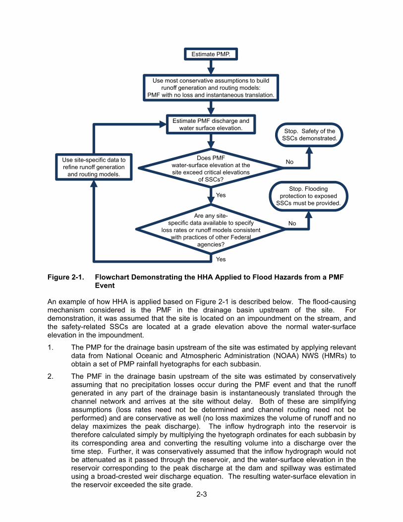
2-3
Figure 2-1. Flowchart Demonstrating the HHA Applied to Flood Hazards from a PMF Event
An example of how HHA is applied based on Figure 2-1 is described below. The flood-causing mechanism considered is the PMF in the drainage basin upstream of the site. For demonstration, it was assumed that the site is located on an impoundment on the stream, and the safety-related SSCs are located at a grade elevation above the normal water-surface elevation in the impoundment.
1. The PMP for the drainage basin upstream of the site was estimated by applying relevant data from National Oceanic and Atmospheric Administration (NOAA) NWS (HMRs) to obtain a set of PMP rainfall hyetographs for each subbasin.
2. The PMF in the drainage basin upstream of the site was estimated by conservatively assuming that no precipitation losses occur during the PMF event and that the runoff generated in any part of the drainage basin is instantaneously translated through the channel network and arrives at the site without delay. Both of these are simplifying assumptions (loss rates need not be determined and channel routing need not be performed) and are conservative as well (no loss maximizes the volume of runoff and no delay maximizes the peak discharge). The inflow hydrograph into the reservoir is therefore calculated simply by multiplying the hyetograph ordinates for each subbasin by its corresponding area and converting the resulting volume into a discharge over the time step. Further, it was conservatively assumed that the inflow hydrograph would not be attenuated as it passed through the reservoir, and the water-surface elevation in the reservoir corresponding to the peak discharge at the dam and spillway was estimated using a broad-crested weir discharge equation. The resulting water-surface elevation in the reservoir exceeded the site grade.
Estimate PMP.
Use most conservative assumptions to build runoff generation and routing models:
PMF with no loss and instantaneous translation.
Estimate PMF discharge and water surface elevation.
Does PMFwater-surface elevation at the site exceed critical elevations
of SSCs?
No
Yes
Are any site-specific data available to specify
loss rates or runoff models consistent with practices of other Federal
agencies?
Use site-specific data to refine runoff generation
and routing models.
No
Yes
Stop. Safety of the SSCs demonstrated.
Stop. Flooding protection to exposed
SSCs must be provided.
2-4
Because the safety-related SSC would be inundated by the flood estimated under extremely conservative conditions, in the second iteration the analysis was made more site-specific by introducing reservoir routing, while keeping all other assumptions the same. The initial water-surface elevation in the reservoir was assumed to be at the full-pool level. Site-specific reservoir storage-elevation-discharge data were used in the reservoir routing. The reservoir routing of the inflow hydrograph reduced the peak discharge at the dam and spillway and resulted in a water-surface elevation that was lower than that computed previously. However, the site was still inundated, although to a lesser degree.
In the third iteration, the assumption of instantaneous translation of the runoff from each subbasin to the reservoir was replaced by runoff generation according to site-specific unit hydrographs adjusted to account for non-linear basin response during large floods approaching the PMF (see Section 2.2). The unit hydrographs reduced the peak discharges from those computed in the first iteration and introduced a time delay or lag between the time when runoff was generated in each subbasin and when it arrived in the channel network. The inflow hydrograph was routed through the reservoir as in the second iteration. The resulting peak water-surface elevation at the site was now below the site grade. Because all safety-related SSCs are located at the site grade, the site is dry under the stillwater effects of the PMF. Notice that two conservative assumptions in the PMF analysis still remain: (1) no precipitation loss and (2) no channel routing. Therefore, the PMF is estimated using a conservative and a relatively simple approach. Coincident wind waves should now be estimated at the site based on the longest fetch length and a 2-year wind and added to the PMF stillwater elevation at the site. If the combined-effects flood water-surface elevation does not exceed the site grade, the site has been demonstrated to be dry. If the combined-effects flood water-surface elevation exceeds the site grade, more site-specific data may be used to characterize channel routing or specify an appropriate yet conservative precipitation loss rate.
3. If the site were determined to be dry, specification of no other design bases for flood hazards from a PMF event would be needed. If the site were determined to be wet even after using all available site-specific data, flooding protection options should be specified for affected safety-related SSCs.
3-1
3 CAUSATIVE MECHANISMS FOR DESIGN-BASIS FLOODS
Several flooding mechanisms or causes, and reasonable combinations of those mechanisms or causes, should be investigated to estimate the design-basis flood at nuclear power plant sites. These mechanisms or causes are described in this chapter.
3.1 Alternative Conceptual Models
Before investing a significant effort involving the simulation of a design-basis flood at a site, it is useful to articulate clearly the alternative conceptualizations of the hydrometeorological phenomena and how they may affect the site. These alternative conceptualizations of causative mechanisms are called alternative conceptual models for the site, and they should be described for all flooding mechanisms. Alternative conceptual models also clearly demonstrate why a particular conceptualization may be more conservative than another. Alternate conceptual models also clearly demonstrate the need for site-specific data and the use of site-specific data in establishing more refined site-specific models. Therefore, alternative conceptual models form the basis of the HHA approach. As described in Chapter 4, the three iterations performed during the example design-basis flood estimation are simply a set of alternative conceptual models. Each alternative conceptualizes the flood-generation mechanism in the drainage basin above the site with a different level of complexity. The alternative conceptual model that ultimately specified the design basis also was clearly demonstrated to be conservative when the assessment was completed.
The need for site-specific data is expected when estimating a design-basis flood. The diverse set of publicly available data compiled by Federal and State agencies that is relevant for estimating design-basis floods is described in Appendix A.
3.2 Local Intense Precipitation
Local intense precipitation is a measure of the extreme precipitation at a given location. The duration of the event and the support area are needed to qualify an extreme precipitation event fully. Generally, the amount of extreme precipitation decreases with increasing duration and increasing area.
The PMP values for areas of the United States east of the 105th meridian are presented in HMRs 51 (Schreiner and Riedel 1978) and 52 (Hansen et al. 1982). The 1-hr, 2.56-km2 (1-mi2) PMP was derived using single-station observations of extreme precipitation, coupled with theoretical methods for moisture maximization, transposition, and envelopment. HMR 52 recommended that no increase in PMP values for areas smaller than 2.56 km2 (1 mi2) should be considered over the 1-hr, 2.56-km2 (1-mi2) PMP. The local intense precipitation is, therefore, deemed equivalent to the 1-hr, 2.56-km2 (1-mi2) PMP at the location of the site.
3.2.1 Flood Generated by Local Intense Precipitation and Its Effects
The elevation of the site, or the site grade, is irrelevant for mitigation of flooding from local intense precipitation. The runoff carrying capacity of the site grading design and the performance of any active or passive drainage system would determine the depth and velocity of surface runoff at the site. Typically, any active drainage systems should be considered non-functional at the time of the local intense precipitation event. The surface runoff would be
3-2
carried off from the immediate powerblock area to any adjoining drainage channels through overland flow and then be carried away from the site to a natural creek or stream.
The runoff losses should be ignored during the local intense precipitation event to maximize the runoff from the event. The powerblock area where safety-related SSCs are located may be subdivided into sub-areas that drain in different directions depending on the site grading design. The hydraulic parameters that affect the depth and velocity of flow should be chosen carefully and should be consistent with values used in standard engineering practice by Federal agencies and other authorities responsible for similar design considerations. The reasons for parameter-value choices should be properly documented.
Hydrologic and hydraulic simulation models accepted in standard engineering practice by Federal agencies and other authorities responsible for similar design considerations may be used to estimate the time history of runoff and its hydraulic characteristics during an event. At the time this report was written, hydrologic and hydraulic simulation models developed, described, and maintained by the Hydrologic Engineering Center (HEC) of the USACE were acceptable to NRC (USACE 2008a, b). Considerations involved in the choice of a simulation model are described in more detail in Chapter 5 of this report. Although this report uses HEC models to illustrate the estimation of floods generated by local intense precipitation at nuclear power plant sites, appropriate justification for selection of methods, data, and models would depend on site-specific circumstances (see Sections 5.3 and 5.4).
If a flood generated by local intense precipitation is determined to be the design basis, each safety-related SSC that may be exposed to the static and dynamic effects of the flood should have openings and doors located above the highest water-surface elevation attained during the event. In addition, the safety-related SSCs should be able to withstand the dynamic effects of the flood (e.g., drag forces). If either of the above conditions is not met, flooding protection for affected safety-related SSCs should be considered and described. If flooding protection is needed for safety-related SSCs, the rate of rise of the flood waters also should be determined to establish available lead times.
3.2.2 Hierarchical Hazard Assessment Applied to a Local Intense Precipitation-Generated Flood
Appendix B provides an example of the method used to estimate flooding in a hypothetical passive site drainage network during a local intense precipitation event. This section describes how the example provided in Appendix B should be applied in the HHA framework using alternative conceptual models of the site drainage.
The simplest and most conservative conceptual model for site drainage is to assume that no active components remain functional and even the passive site drainage network is compromised. This conceptual model corresponds to Case 3 described in Appendix B. The method described there should be used to determine the highest water-surface elevation during the local intense precipitation event. If the estimated water-surface elevation does not affect any safety-related SSCs, it can be concluded that the plant would be safe from the effects of the local intense precipitation event.
If the water-surface elevation estimated using Case 3 does result in adverse effects to one or more safety-related SSCs, and site constraints would not allow for adequate modifications to the grading or placement of the SSCs, the conceptual model described in Case 2 could be used. However, a clearly articulated justification, supported by site-specific hydrometeorological data, would be needed to demonstrate that the passive site drainage network would not be
3-3
completely blocked by debris or otherwise compromised during the local intense precipitation event. Once the justification has been documented, the methods used in Case 2 may be used to estimate the water-surface elevation during the local intense precipitation event.
If the water-surface elevation estimated using Case 2 results in adverse effects on one or more safety-related SSCs, the methods described in Case 1 may be used. However, hydrometeorological evidence suggests it is extremely rare that the passive site drainage network would remain completely unblocked during a local intense precipitation event. Therefore, use of this conceptual model is not recommended. Instead, the site grade and the drainage network may need to be redesigned.
3.3 Flooding in Rivers and Streams
The PMF in rivers and streams adjoining the site should be determined by applying the PMP to the drainage basin of these rivers and streams. The PMF is defined by ANSI/ANS-2.8-1992 (ANS 1992) as “… the hypothetical flood (peak discharge, volume, and hydrograph shape) that is considered to be the most severe reasonably possible, based on comprehensive hydrometeorological application of PMP and other hydrologic factors favorable for maximum flood runoff such as sequential storms and snowmelt.”
3.3.1 Estimating the PMF and Its Effects
The estimation of PMP for different zones of the United States has been described by NOAA NWS in its series of HMRs. The PMP is a deterministic estimate of the theoretical maximum depth of precipitation that can occur at a time of year over a specified area. A rainfall-to-runoff transformation function and an accounting of the runoff aggregation by the topographic and drainage or stream network characteristics in addition to certain watershed properties are needed to estimate the PMF hydrograph. Simulation models called “hydrological models” typically use the time history of PMP precipitation as input and estimate the PMF runoff hydrograph given a set of watershed parameters that describe precipitation losses, rainfall-to-runoff transformation, antecedent streamflow conditions, and travel time within the stream network.
A PMF hydrograph obtained from hydrological models provides only a time history of discharge or streamflow within the stream network. To obtain the hydraulic parameters of the PMF, such as velocity and depth, another class of models usually called “hydraulic models” is used. The hydraulic models use the PMF hydrographs estimated by hydrological models at key locations, a set of physical properties of the stream network such as longitudinal and cross-sectional geometry, stream reach connectivity, channel roughness, and initial conditions within the stream network to estimate PMF flow velocities and depths (or equivalently, the flood water-surface elevation).
The hydraulic properties estimated by the hydraulic model are used then to specify the PMF characteristics near the site. If the water-surface elevation in the river or stream adjacent to the site exceeds the design site grade, the static and dynamic effects of the PMF may adversely affect safety-related SSCs. The affected SSCs should be protected from the most severe hazards, or the site grade should be redesigned. Regulatory Guide 1.102 (NRC 1976) describes the types of flooding protection acceptable to the NRC.
At the time this report was written, hydrologic and hydraulic simulation models developed, described, and maintained by the USACE HEC were acceptable to the NRC. Considerations that should be applied when choosing a simulation model are described in more detail in
3-4
Chapter 5 of this report. Although this report uses HEC models to illustrate the estimation of floods in river and streams that may affect nuclear power plant sites, appropriate justification for selection of methods, data, and models would depend on site-specific circumstances (see Sections 5.3 and 5.4).
If the PMF is determined to be the design basis, each safety-related SSC that may be exposed to the static and dynamic effects of the PMF should have its openings and doors located above the highest water-surface elevation attained during the event. In addition, the safety-related SSCs should be able to withstand the dynamic effects of the PMF (e.g., drag forces). If either of the above conditions is not met, flooding protection for affected safety-related SSCs should be considered and described. If flooding protection is needed for safety-related SSCs, the rate of rise of the flood waters also should be determined to establish available lead times for responding to floods.
3.3.2 Hierarchical Hazard Assessment Applied to PMF
Appendix C provides an example of how to estimate the PMF at a hypothetical nuclear power plant site. An example of the use of alternative conceptual models within the HHA framework to estimate the design-basis flood from a PMF is provided in Section C.4. Appendix C contains additional discussions regarding alternative conceptual models that should be investigated (see discussion of scenarios in Section C.4).
The most commonly accepted way of specifying a rainfall-runoff transformation function accepted is the unit hydrograph approach, which was proposed by Sherman (1932). The unit hydrograph is defined as the direct runoff hydrograph that results from a unit depth of spatially and temporally uniform rainfall excess in the drainage basin over a specific duration (Pilgrim and Cordery 1993).
The theory behind the unit hydrograph approach is based on two assumptions: (1) the drainage basin is a lumped system in that no spatial variability in rainfall input or losses is allowed, and (2) the direct runoff discharge hydrograph for rainfall excess values other than the unit depth can be obtained simply by scaling the unit hydrograph ordinates by the rainfall excess value. The direct runoff hydrograph from a sequence of rainfall excess depth is calculated by superimposing the individual responses from each of the individual pulses of rainfall excess. Because of the linearity assumption, unit hydrographs of other durations can be estimated readily if a unit hydrograph of a given duration is available (Chow et al. 1988).
Unit hydrographs can be estimated from observed rainfall and runoff data (Chow et al. 1988). For ungauged drainage basins, empirical relationships based on characteristics of the drainage basin have been developed to estimate synthetic unit hydrographs (e.g., NRCS 1985; Nash 1960; Snyder 1938; Clark 1945). Standard hydrology texts, such as Chow et al.’s (1988), contain descriptions of these methods. More recent research has attempted to derive unit hydrographs from geomorphic characteristics of the drainage basin (Rodriguez-Iturbe and Valdes 1979; Gupta et al. 1980; Rodriguez-Iturbe and Rinaldo 1997).
One vexing problem remains when using unit hydrographs to estimate the PMF. By definition, the PMF is an extremely rare event, with virtually no possibility of being exceeded. Therefore, unit hydrographs derived from observed rainfall and runoff data, or those based on empirical relationships, do not represent hydrometeorological conditions that would prevail during a flood as large as the PMF. The hydraulic efficiency of drainage networks is expected to increase during a PMF event, and the flood discharge is certain to overflow the banks of drainage channels and occupy large areas of the floodplain. For these reasons, the drainage basin
3-5
response during a PMF event is expected to be much different from that assumed during the derivation of the unit hydrographs, violating the linearity assumption in the theory. At the very least, the unit hydrographs should be derived from floods that are among the largest on record and that approach the magnitude of the PMF. Pilgrim and Cordery (1993) describe a set of adjustments that may be made to unit hydrographs derived from floods smaller than the PMF. The recommended adjustments to peak discharge and lag time (i.e., the time to peak discharge) are a 5-to-20-percent increase for the peak discharge and a 33-percent reduction in the lag time.
3.4 Dam Breaches and Failures
Flood waves resulting from severe breaches of upstream dams, including domino-type or cascading dam failures, should be evaluated for the site. Water-storage or water-control structures (such as onsite cooling or auxiliary water reservoirs and onsite levees) that may be located at or above the safety-related site grade should also be evaluated. In cases of failure of earthen levees or embankments onsite, the effects of sediment being carried with the flood wave should also be determined.
Dam failure scenarios, particularly those related to cascading dam failures, should be carefully analyzed and documented to establish that the most severe of the possible combinations has been accounted for. Typically, two scenarios of upstream dam failure should be considered: (1) failure of individual dams and (2) cascading or domino-like failures of dams. Appendix D provides an example of cascading combinations and methods for estimating the geometric characteristics of dam breaches.
3.4.1 Hierarchical Hazard Assessment Applied to Dam Breaches and Failures
The simplest and most conservative dam-breach induced flood may be expected to occur under the assumption that (1) all dams upstream of the site are assumed to fail during the PMF event regardless of their design capacity to safely pass a PMF and (2) the peak discharge from individual dam failures reach the site at the same time. In this scenario, the peak discharges of all individual flood waves from the failures, augmented by PMF inflows, arrive at the site at the same time. This scenario is clearly the most conservative because (1) PMF is augmented by release of stored water within the reservoirs and (2) differences in travel time for the peak discharges from individual dam failures to reach the site is ignored.
If the flood water-surface elevation in the stream adjacent to the site from the most conservative scenario described above when combined with wind-induced waves is below the safety-related site grade, no further analysis would be necessary. If the safety-related site grade is exceeded, site-specific data may be used to specify progressively more refined scenarios of dam failures:
1. Investigate the failures of only a subset of all the upstream dams while assuming that peak discharges of individual dam-failure induced floods reach the site at the same time. A justification that the remaining dams would not fail under PMF scenarios should be provided.
2. The most severe cascading failure combination should be investigated (see Appendix D for an example). This scenario may require setting up the USACE Hydrologic Engineering Center River Analysis System (HEC-RAS) model or another hydraulic model input with site-specific data related to channel geometry and bathymetry and reservoir stage-storage-discharge relationships. Manning’s roughness coefficients also would be needed as input. An example of this approach is provided in Appendix D.
3-6
Although this report uses HEC models to illustrate the estimation of floods from dam breaches and failures that may affect nuclear power plant sites, appropriate justification for selection of methods, data, and models would depend on site-specific circumstances (see Sections 5.3 and 5.4).
If the dam-failure induced flood is determined to be the design basis, each safety-related SSC that may be exposed to the static and dynamic effects of the flood should have openings and doors located above the highest water-surface elevation attained during this event. In addition, the safety-related SSC should be able to withstand the dynamic effects of the flood (e.g., drag forces). If either of the above conditions is not met, flooding protection for affected safety-related SSCs should be considered and described. If flooding protection is needed for safety-related SSCs, the rate of rise of the flood waters also should be determined to establish available lead times.
Sunny-day failure of dams, which are characterized by an absence of a concurrent extreme flood, may produce the highest flood elevations depending on the relative location of the dam, water-surface elevation in the reservoir, and the critical elevations of safety-related SSCs. These dam failures may occur due to failures of embankment material or foundation such as those due to piping through the embankment or liquefaction of foundation during seismic events. Sunny-day failures of dams could result in single or multiple cascading failures depending on the configuration of the water-storage facilities. The possibility of these failures should be carefully evaluated to ensure that all plausible mechanisms for flooding from dam breaches and failures at and near a site are considered.
3.5 Storm Surge
Storm types are defined by NOAA according to the maximum sustained wind speed. The maximum sustained wind speed is defined as the highest 1-minute average wind speed within the storm at a height of 10 m (33 ft).
Tropical storms in the Atlantic Ocean start as tropical disturbances, which are weather systems with an apparently organized convection around a low pressure center and movement that is sustained for a day or more. As the central pressure drops, the weather system can sustain faster winds and develop into a tropical depression that is characterized by maximum sustained wind speeds up to 61 km/hr (38 mph, 33 kt). The weather system strengthens into a tropical storm if the maximum sustained winds reach speeds of 63 to 117 km/hr (39 to 73 mph, 34 to 63 kt). Further strengthening of the storm categorizes it as a hurricane. As shown in Table 2.1, the Saffir-Simpson hurricane intensity scale (Simpson and Riehl 1981) is used by NOAA to describe the severity of hurricanes in five categories. The use of central pressure as a defining characteristic was discontinued in the 1990s.
Storm surge is the rise in offshore water elevation caused principally by the shear force of the hurricane winds acting on the surface. A secondary rise in water surface is also caused by the lowering of the air pressure within the hurricane. In the past, the Saffir-Simpson scale also was used to describe expected storm surges from hurricanes of different categories. Irish et al. (2008) point out that while the use of Saffir-Simpson scale is appropriate for wind damage, its use as an indicator for storm surge is not. Using numerical simulations of idealized hurricanes, they showed that storm intensity, bottom slope, and storm size are important factors in storm surge generation at the coastline. Simulated storm surge increased with storm size for a given storm intensity (Irish et al. 2008).
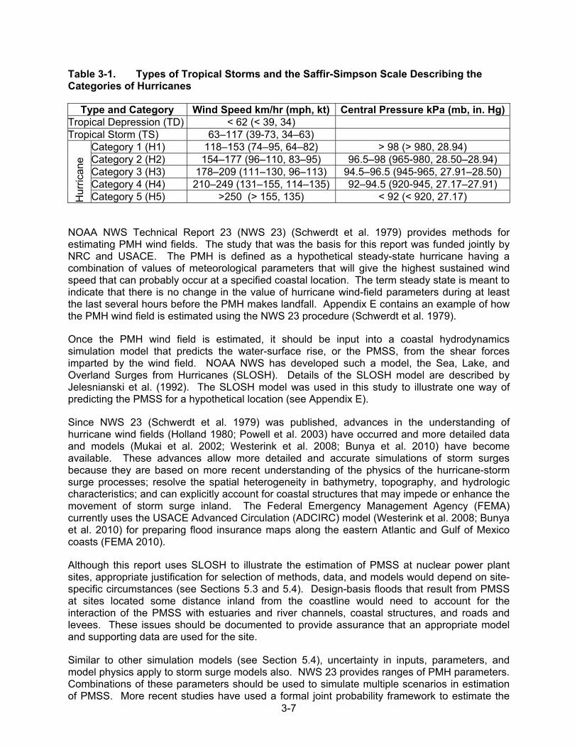
3-7
Table 3-1. Types of Tropical Storms and the Saffir-Simpson Scale Describing the Categories of Hurricanes
Type and Category Wind Speed km/hr (mph, kt) Central Pressure kPa (mb, in. Hg)Tropical Depression (TD) < 62 (< 39, 34) Tropical Storm (TS) 63–117 (39-73, 34–63)
Hur
rican
e
Category 1 (H1) 118–153 (74–95, 64–82) > 98 (> 980, 28.94) Category 2 (H2) 154–177 (96–110, 83–95) 96.5–98 (965-980, 28.50–28.94) Category 3 (H3) 178–209 (111–130, 96–113) 94.5–96.5 (945-965, 27.91–28.50) Category 4 (H4) 210–249 (131–155, 114–135) 92–94.5 (920-945, 27.17–27.91) Category 5 (H5) >250 (> 155, 135) < 92 (< 920, 27.17)
NOAA NWS Technical Report 23 (NWS 23) (Schwerdt et al. 1979) provides methods for estimating PMH wind fields. The study that was the basis for this report was funded jointly by NRC and USACE. The PMH is defined as a hypothetical steady-state hurricane having a combination of values of meteorological parameters that will give the highest sustained wind speed that can probably occur at a specified coastal location. The term steady state is meant to indicate that there is no change in the value of hurricane wind-field parameters during at least the last several hours before the PMH makes landfall. Appendix E contains an example of how the PMH wind field is estimated using the NWS 23 procedure (Schwerdt et al. 1979).
Once the PMH wind field is estimated, it should be input into a coastal hydrodynamics simulation model that predicts the water-surface rise, or the PMSS, from the shear forces imparted by the wind field. NOAA NWS has developed such a model, the Sea, Lake, and Overland Surges from Hurricanes (SLOSH). Details of the SLOSH model are described by Jelesnianski et al. (1992). The SLOSH model was used in this study to illustrate one way of predicting the PMSS for a hypothetical location (see Appendix E).
Since NWS 23 (Schwerdt et al. 1979) was published, advances in the understanding of hurricane wind fields (Holland 1980; Powell et al. 2003) have occurred and more detailed data and models (Mukai et al. 2002; Westerink et al. 2008; Bunya et al. 2010) have become available. These advances allow more detailed and accurate simulations of storm surges because they are based on more recent understanding of the physics of the hurricane-storm surge processes; resolve the spatial heterogeneity in bathymetry, topography, and hydrologic characteristics; and can explicitly account for coastal structures that may impede or enhance the movement of storm surge inland. The Federal Emergency Management Agency (FEMA) currently uses the USACE Advanced Circulation (ADCIRC) model (Westerink et al. 2008; Bunya et al. 2010) for preparing flood insurance maps along the eastern Atlantic and Gulf of Mexico coasts (FEMA 2010).
Although this report uses SLOSH to illustrate the estimation of PMSS at nuclear power plant sites, appropriate justification for selection of methods, data, and models would depend on site-specific circumstances (see Sections 5.3 and 5.4). Design-basis floods that result from PMSS at sites located some distance inland from the coastline would need to account for the interaction of the PMSS with estuaries and river channels, coastal structures, and roads and levees. These issues should be documented to provide assurance that an appropriate model and supporting data are used for the site.
Similar to other simulation models (see Section 5.4), uncertainty in inputs, parameters, and model physics apply to storm surge models also. NWS 23 provides ranges of PMH parameters. Combinations of these parameters should be used to simulate multiple scenarios in estimation of PMSS. More recent studies have used a formal joint probability framework to estimate the
3-8
distribution and spatial properties of storm surge in the Gulf of Mexico (Resio et al. 2009; Irish et al. 2009). These methods are still being developed and may require significant effort to implement at specific sites, although some research is also being carried out that may help in reducing the burden (Irish et al. 2009). Some of the issues discussed here can also be addressed in a formal probabilistic flood hazard assessment, as described in Section 5.6, and are recommended for future research.
3.5.1 Hierarchical Hazard Assessment Applied to PMSS
As with the other flood-causing mechanisms described above, the HHA should be applied to flooding from PMSS. However, the application of HHA to PMSS is less straightforward because there are few parameters that need adjustment. The factors that may change the PMSS water-surface elevation at the site are (1) the ambient tide level for coastal and streamside locations and (2) the ambient flood water-surface elevation for the streamside locations. These two factors are accounted for in combined events criteria described below. It is not recommend that the parameters of the SLOSH model be varied because they have been set to values that result in an acceptable predictive accuracy for the U.S. Gulf and the Atlantic Coasts.
For a given location however, the PMH has three variable parameters: (1) the forward speed (T), (2) the radius of maximum winds (R), and (3) the track direction (θ). Because of uncertainty in these parameters, the NWS 23 estimation procedure provides a range of values for these parameters of the PMH wind field.
The NOAA NWS also defines two terms related to the maximum expected water-surface elevation. The maximum envelope of water (MEOW) is defined as the maximum water-surface elevation at any given location during simulation of the storm surge from a given hypothetical hurricane characterized by storm category, track direction, forward speed, and tide level. Therefore, the MEOW at any given location can be thought of as the peak of the water-surface elevation hydrograph for a specific hurricane.
MEOWs can be generated for several hypothetical hurricanes of a specific storm category by varying the track direction, forward speed, and tide level. The maximum of these water-surface elevations at any given location is called maximum of the MEOWs (MOM). Because there are five storm categories defined by the Saffir-Simpson scale, five MOMs exist for any given location.
The PMH does not have a Saffir-Simpson category assigned to it. However, MEOWs for a PMH can still be generated by simulating the PMSS for a specific set of T, θ, and R. Because each of these three parameters of the PMH wind field has a range associated with it, a set of hypothetical PMSS simulations can be performed for a given location by varying the three parameters over their stated ranges. From each of these PMSS simulations, a MEOW can be obtained for the site location. The maximum of these MEOWs, therefore, is a PMH MOM.
The approach adopted in this report is to estimate the PMH MOM for the site location (see Appendix E) and then use it as an estimate of the PMSS.
If the PMSS is determined to be the design basis, each safety-related SSC that may be exposed to the static and dynamic effects of the flood should have openings and doors located above the highest water-surface elevation attained during this event. In addition, the safety-related SSCs should be able to withstand the dynamic effects of the flood (e.g., drag forces). If either of the above conditions is not met, flooding protection for affected safety-related SSCs
3-9
should be considered and described. If flooding protection is needed for safety-related SSCs, the rate of rise of the flood waters also should be determined to establish available lead times.
3.6 Seiche
A seiche is defined as an oscillation of the water surface in an enclosed or semi-enclosed body of water initiated by an external cause (Wüest and Farmer 2003; Scheffner 2008). Once started, the oscillation may continue for several cycles; however, over time it gradually decays because of friction.
The period of oscillation of seiches can vary from a few minutes in bays to more than 10 hours in the Great Lakes; resonance may occur in Great Lakes for periods between 2 to 10 hours (Scheffner 2008).
In the HHA framework, the first step is to determine whether a seiche in a nearby lake or reservoir can potentially lead to flooding at the site. A method for determining if a seiche can be initiated by an external meteorological or seismic forcing for basins of simple geometry is described in Appendix F. However, significant errors may be introduced when determining fundamental oscillation periods if a complex basin geometry and bathymetry is represented by an idealized rectangular basin of constant depth.
For lakes and bays that have irregular geometries and variable bathymetries, numerical, long-wave hydrodynamic modeling may be the only viable solution. If the margin between the site grade and the normal water level in an adjacent waterbody subject to seiches is small, numerical modeling may need to be used to assess the flooding hazard from severe seiches. Scheffner (2008) describes model selection criteria and references to an example. Another example is described by Stevens and Lawrence (1997).
If a seiche is determined to be the design basis, each safety-related SSC that may be exposed to the static and dynamic effects of the flood should have openings and doors located above the highest water-surface elevation attained during this event. In addition, the safety-related SSCs should be able to withstand the dynamic effects of the flood (e.g., drag forces). If either of the above conditions is not met, flooding protection for affected safety-related SSCs should be considered and described. If flooding protection is needed for safety-related SSCs, the rate of rise of the flood waters also should be determined to establish available lead times.
3.7 Ice-Induced Flooding
Ice jams and ice dams can form in rivers and streams adjacent to a site and may lead to flooding by two mechanisms: (1) collapse of an ice jam or a dam upstream of the site can result in a dam breach-like flood wave that may propagate to the site and (2) an ice jam or a dam downstream of a site may impound water upstream of itself, thus causing a flood via backwater effects.
While it is possible to assess whether a site may possess hydroclimatic conditions that are precursors to ice-jam or ice-dam formation (see Appendix G), it is not possible to predict the exact location and severity (e.g., the width, height, and volume) of the ice blockage accurately. Therefore, it is not possible, at this time, to predict a probable maximum ice jam or dam accurately. Alternatively, it is recommended that historical records of ice jams and dams be searched to determine the most severe historical event in the vicinity of the site.

3-10
In the HHA framework, it may be possible to determine whether a flood caused by another flood-causing mechanism at or near the site may exceed that resulting from an ice event. If such an alternative and bounding flood is found, no further analysis for the ice-induced flood is necessary. If such a bounding flood is not found for the site, methods described in Appendix G should be used to estimate the flood water elevation and other associated hazards for the most severe historical ice jam or ice dam event. Because this event is not a probable maximum event, but merely the most severe historically observed event, care should be exercised in specifying a significant margin between the estimated maximum flood water-surface elevation and the site grade.
If an ice event is determined to be the design basis, each safety-related SSC that may be exposed to the static and dynamic effects of the flood should have openings and doors located above the highest water-surface elevation attained during the event. In addition, the safety-related SSC should be able to withstand the dynamic effects of the flood (e.g., drag forces). If either of the above conditions is not met, flooding protection for affected safety-related SSCs should be considered and described. If flooding protection is needed for safety-related SSCs, the rate of rise of the flood waters also should be determined to establish available lead times.
3.8 Flooding Resulting from Channel Migration or Diversion
Natural channels may migrate or divert either away from or toward the site. The relevant event for flooding is diversion of water towards the site. There are no well-established predictive models for channel diversions. Therefore, it is not possible to postulate a probable maximum channel diversion event. Instead, historical records and hydrogeomorphological data should be used to determine whether an adjacent channel, stream, or river has exhibited the tendency to meander towards the site.
Relevant data sources for this investigation include channel form, historical topographic maps, soil types, geologic characteristics, and other morphological parameters. Because most channel diversion occurs during high flows when the stream or river overflows its banks, flood data, particularly stage, may also prove useful in the determination.
Generally, stream channels that are steeply incised, have limited floodplains, and are located in geologic formations relatively resistant to erosion would not be expected to be susceptible to channel diversion. If a site is indeed subject to such an event, the site generally should be determined to be unsuitable for a nuclear power plant.
Man-made channels, canals, diversions, and levees used for conveyance of water and flood protection may also be located near the site. During extreme floods, these facilities can fail and result in diversion of water towards the site. Therefore, all water-conveyance and water-storage facilities near the site should be carefully evaluated to ensure their effects are accounted for in determination of the design-basis flood at the site.
3.9 Combined-Effects Flood
The ANS states that a single flood-causing event is inadequate as a design basis for power reactors (ANS 1992). Dependent events can occur concurrently (e.g., precipitation, snowpack, and wind waves; high tides, and storm surges). Currently, the design-basis flood at a nuclear power plant site is estimated from deterministic approaches that use the notion of a probable maximum event. Despite the term “probable,” probable maximum events are thought to approach the physical limits of the phenomena, are deterministic in nature, and are thought to

3-11
exceed all historical occurrences of the phenomena. There are no consistent, well-established methods for estimating the probability-of-exceedance of probable maximum events.
Because of their extreme nature, probable maximum events from two separate phenomena should not be combined unless they are clearly dependent or result from a common cause. For example, seismic events should not be combined with precipitation events. An exception occurs for PMF and PMH for relatively small drainage basins in regions where the PMP may result from a hypothetical and maximized hurricane event. Wind waves are almost always combined with other flood-causing mechanisms. Details of the combinations are provided in Appendix H.
The combination that results in the most severe flood hazard to the safety-related SSCs is used to specify the design basis. It is worth noting here that different flood hazards may occur from different combinations. For example, the maximum water-surface elevation, and consequently the maximum hydrostatic force, may result from a PMF combined with wind waves, but the maximum hydrodynamic force may result from fast-moving waters of a PMT. Therefore, design-basis events should be chosen for each case to establish sufficient safety margins for each of the most severe loadings possible.
Because events can occur in combination, a formal probabilistic flood hazard assessment approach can provide a more consistent treatment of combination of events that are consistent with local and regional hydrometeorological characteristics. An extended discussion of this subject is not the focus of this report.

4-1
4 APPROACHES
This chapter describes the two analytical approaches used in standard engineering practice for estimating design-basis floods: deterministic analysis and probabilistic analysis. The emphasis is placed on methods used to estimate design-basis floods at nuclear power plant sites, but the conceptual bases for these models are generally applicable for other purposes also.
Because the safety-related SSCs of a nuclear power plant may be exposed to a range of flood-related hazards, the term “design-basis flood” should more accurately be thought of as a set of “design-basis flood hazards.” Some of these hazards include hydrostatic and hydrodynamic forces, erosion and deposition potential, and impacts from debris carried by a flood. It also is important to note that individual, worst-case flood hazards may result from different flooding mechanisms. Therefore, it may not be appropriate to focus on a single “design-basis flood;” rather, the design should consider the worst-case hazards resulting from all appropriate combined-effects floods that are relevant for a site and the nuclear power plant SSCs.
The deterministic approach, currently used for nuclear power plant sites in the United States, is based on the premise that floods can be estimated from a set of empirical or physical prediction relationships. Often, a combination of empirical and physical relationships also may be used in a flood-prediction model. Usually, deterministic approaches try to predict the flood hazards for a hypothetical worst-case hydrometeorological event. For example, predicting the PMF in stream and rivers uses the PMP as input along with hydrological conditions in the affected drainage area aim to maximize runoff from the PMP. The hazards caused by the PMF and those caused by other flood-causing mechanisms would then be used as the set of hazards from which the design bases should be selected.
As its name indicates, the second approach uses probabilistic techniques to estimate the flood hazards corresponding to a specified probability-of-exceedance. The probabilistic techniques are based on an assumption that extreme floods follow a probability distribution whose parameters can be estimated within a certain degree of confidence from past observations. The estimated probability distribution of the extreme flood then may be used to derive the probability distribution of the individual hazards caused by extreme floods. The probability distributions of the individual hazards may then be used to select a design basis corresponding to a selected probability-of-exceedance. Because historical data for extreme events are limited by the extent of the observed record, probabilistic techniques may be subject to significant uncertainty in the estimated hazard magnitudes.
4.1 Deterministic Analyses
Deterministic analyses to predict floods often use empirical and physical prediction relationships implemented into flood simulation models. The predictions are “deterministic” in the sense that given a particular set of inputs, the prediction is always the same and uncertainty in inputs and model parameters are generally not considered explicitly. Consequently, to gain confidence in model predictions for estimating design-basis flood hazards, the parameters of the model may need to be calibrated using data on large historical floods and then validated on comparatively large flood events not used in the calibration.
The simplest of the deterministic flood prediction models is the rational method, which is based on the following formula:
· · (1)
4-2
where Qt is the flood discharge at the outlet (dimension of [L3T-1]) at time t, it is the precipitation intensity (dimension of [LT-1]), and A is the contributing drainage area (dimension of [L2]). The term C is the dimensionless runoff coefficient that embeds the effects of precipitation losses, runoff generation, and watershed transformation processes within itself. Notice that it and Qt are time series (i.e., precipitation hyetograph and discharge hydrograph, respectively). It is worth noting here that the rational method assumes that the precipitation is spatially uniform over the drainage area A, and the precipitation excess (precipitation minus losses) is instantaneously transformed into runoff. The rational method may be used for small, urban, or mostly impervious drainage areas to estimate the flood discharge conservatively.
More complicated deterministic hydrologic models can be thought of as variations of the rational method where the effects of hydrological processes are conceptualized in more detailed sub-models. For example, if the drainage area is large enough that spatial uniformity of precipitation is not a valid assumption, the drainage area may be subdivided into several subbasins that are small enough to justify the assumption of uniformity of rainfall within themselves. This approach essentially leads to “spatially distributed” hydrological models where inputs (e.g., precipitation and air temperature) and model parameters (e.g., runoff coefficient) vary among the subbasins. If the drainage area were divided into n subbasins with each having its own precipitation input and runoff coefficients, the rational method may be implemented using the following formula:
∑ ∑ · · (2)
where the subscript j refers to the jth subbasin and ∑ is the total drainage area ([L2]). The model now needs estimates of precipitation and runoff coefficients for each subbasin. However, precipitation excess is still transformed instantaneously into runoff regardless of the distance between a particular subbasin and the outlet. The variation in the travel time for each subbasin’s runoff to reach the outlet also can be accounted for by staggering the runoff generated from each subbasin in time; in effect accounting for channel routing. Accounting for these individual complexities in the runoff generation and delivery processes quickly becomes so complicated that closed-form expressions of the discharge at the outlet, such as those described above, are not possible. Therefore, more complicated hydrologic models are assembled from modular mathematical and numerical representations of hydrological process descriptions. However, deterministic models assume that inputs are perfectly known and contain no measurement errors, the model parameters (e.g., the runoff coefficient) can be measured perfectly or estimated, and the process representations do not change with scale, either in space or in time.
Deterministic models, depending on their complexity, require data to estimate parameters accurately. Therefore, these models should be used carefully to ensure consistency with available site-specific data.
The rational method and its variations described above are typically referred to as empirical models, which are derived from observations that the rate of discharge at the outlet of the drainage basin may be approximately proportional to the rate of rainfall. Another class of deterministic models also exists. These models, called physically-based process models, describe the physics of the hydrological processes and assemble these descriptions into the model. Typically, hydrological processes are described mathematically on a small spatial scale, and model parameters may be estimated based on experiments at the laboratory scale or the field scale. Hydrological processes commonly included in such models include partitioning of precipitation into rain or snow, interception of precipitation by vegetation canopy, snow accumulation and melt on the surface, infiltration of snowmelt or through-fall (i.e., rainfall that is not intercepted by the vegetative canopy) into the soil, evapotranspiration, surface runoff
4-3
generation, recharge of deep soil layers and base-flow generation, and channel routing to the outlet of the basin. An example of such a model is the Distributed Hydrology Soil-Vegetation Model (Wigmosta et al. 1994, 2002; Doten et al. 2006). However, these models are used mostly for research purposes and require an extensive amount of site-specific data.
Simpler process models that strike a balance between the extreme simplicity of the rational method and the relative complexity of the physically-based process models have been widely used also. These models are called lumped-parameter models. The process descriptions are developed and implemented on a subbasin scale, and variations in model parameters among subbasins are allowed. Typical components of these models include accounting for precipitation losses, a transformation function (to estimate the runoff response from the subbasin for a given precipitation excess), a description of channel-network connectivity, effects of possible dams or other water-control structures, and channel routing. The most widely used lumped-parameter model is the USACE Hydrologic Engineering Center Hydrologic Modeling System (HEC-HMS) (USACE 2008b; 2009b). More details of the HEC-HMS model and its application to estimating design-basis flood hazards are given in Appendix C.
The hydrologic models described above assist in estimating the discharge hydrographs at points of interest. The hazards from flooding also require development of estimates of the hydraulic properties of the design-basis flood discharge (e.g., the water-surface elevation in the river, velocity of the flow in the river near the site, hydrodynamic forces, etc.). To estimate these properties, hydraulic models that describe the dynamics of discharge in the river or stream need to be used. Hydraulic models are usually implemented to solve simplified forms of the governing equations for gradually varied, unsteady flow in open channels (Chow 1959). The most widely used of these models is the USACE HEC-RAS (USACE 2008a; 2009c). More details of the HEC-RAS model and its application to estimating design-basis flood hazards are given in Appendix D. Depending on the particular configuration of the stream reaches being modeled, hydraulic models require geometry and hydraulic data, including channel cross sections, channel roughness data, and reservoir stage-storage-discharge data.
4.2 Probabilistic Analyses
Probabilistic models for estimating design-basis floods are generally based on approaches that characterize the extreme flood as a random event, describe the properties of this random phenomenon using probability distributions, and use these probability distributions to estimate extreme floods corresponding to a specified probability-of-exceedance (Stedinger et al. 1993).
The two key components of the probabilistic models are (1) the historical flood data and (2) the probability distribution used to describe the historical flood data. Typically, the historical record of annual maximum instantaneous peak discharge at the site of interest, usually measured by a United States Geological Survey (USGS) streamflow gauge, is used to estimate the probability distribution of extreme floods. Because the random variable of interest—the peak discharge—is represented as a continuous variable, a continuous probability distribution is appropriate.
Probability distributions may be represented by a closed-form, parametric probability density function (PDF) or by a data-centric, nonparametric PDF. Parametric PDFs use a functional form or an equation to represent the shape of the distribution. For example, the normal distribution is represented by the following PDF (Haan 1977):
√ (3)
4-4
where x is the random variable, μ is the mean, and σ is the standard deviation of the random variable. Because the parameters μ and σ control the location and the shape of the normal distribution, respectively, they are also referred to as the location and scale parameters of the distribution.
A continuous PDF must satisfy two conditions: (1) the integral of the PDF over all possible values of the random variable must equal 1, and (2) its value corresponding to all values of the random variable must be non-negative.
A nonparametric PDF cannot be expressed in a function form such as that shown above. Usually, nonparametric PDFs are constructed by placing a kernel at each observation of the random variable (Adamowski 1985; Lall et al. 1993). The main advantages of using nonparametric PDFs are (1) consistency with data, (2) robustness with respect to outliers, and (3) flexibility in shape, especially multi-modality. At this time, nonparametric methods are not applied frequently in standard engineering practice. Although the data-centric nature of the nonparametric methods makes them an attractive alternative, a specific disadvantage is their limited ability to extrapolate beyond observed data (Lall et al. 1993). The extrapolation problem is severe if the chosen kernel used to estimate the PDF is truncated (i.e., has non-zero densities only for a limited range of values of the random variable). For this reason, applications of nonparametric PDFs reported in the flood-frequency literature use kernels that have unlimited support (e.g., the normal, the Cauchy, and the extreme value type I distributions [Lall et al. 1993]).
Bulletin 17B of the Hydrology Subcommittee of the Interagency Advisory Committee on Water Data (IACWD) describes a method for estimating probability distributions for annual peak discharges in the United States (IACWD 1982). The method is based on fitting a parametric PDF, the log Pearson type-III PDF, to the annual maximum instantaneous peak discharge. The method was developed assuming stationarity (i.e., the assumption that relationships existing among variables at present will stay the same) and, therefore, does not account for trends, such as those resulting from climate variability and change. The method also assumes that input data are homogeneous; therefore, IACWD (1982) recommends careful examination of data to identify watersheds where changes may have occurred (e.g., urbanization or construction of dams, levees, and diversions) or to identify whether the annual peak discharge may be produced by multiple mechanisms (e.g., by rainstorms, snowmelt, or a combination of the two).
The procedure recommended by IACWD (1982) consists of the following steps:
1. Perform logarithmic transformation of annual peak discharge data.
2. Estimate sample mean, standard deviation, and coefficient of skew from transformed data.
3. Identify high and low outliers (if outliers are found, they should be removed and the statistics in Step 2 should be recomputed) and compute the weighted coefficient of skew.
4. Compute the coordinates of the frequency curve corresponding to selected probabilities-of-exceedance.
5. Compute the confidence limits for the frequency curve.
IACWD (1982) also describes adjustments for data where some annual peak discharges may be zero (this condition is expected in arid drainage basins that may have no flow during certain years). The USGS has developed a computer program, PeakFQ, that implements the methods described in Bulletin 17B (Flynn et al. 2006). The IACWD (1982) method is currently used in engineering practice.
4-5
The log Pearson type-III probability distribution fit to the observed annual peak-discharge data can be used to estimate the flood discharge for the selected probability-of-exceedance that the design basis would be based on. However, the method yields only a single discharge and the associated confidence band on that discharge, and not a time series. A deterministic hydraulic model may need to be used to estimate the hazards from this discharge. For example, the HEC-RAS program could be set up for the stream reach near a proposed site to estimate the hydraulic properties of a steady-state discharge equal to that obtained from the above procedure. In fact, such a procedure often is used not only for the estimated flood discharge but also for the range of annual peak discharges to create distributions of the hazards resulting from those flood discharges. Essentially, the deterministic hydraulic model acts as a “transformation function” that converts the distribution of the flood discharge into the distributions of the associated hazards. However, careful application of this approach is required because the deterministic hydraulic model itself may contain uncertainties (e.g., the parameters of the model may not be known perfectly). Therefore, the uncertainties in the estimated design-basis flood discharge would be compounded by uncertainties in the “transformation function,” and the confidence band on the design-basis flood hazard may be larger than that on the design-basis flood discharge. Some of these issues are described in Chapter 5.
Relatively short observation history of streamflow complicates the accurate determination of frequency distribution of extreme floods. To augment recorded history of streamflow, paleo-flood data can be used in frequency estimation of extreme floods (England et al. 2003; Swain et al. 2004; Griffis and Stedinger 2007). Uncertainty in the estimates of the paleo-flood discharges as well as dating of these events complicates the analysis (O’Connell et al. 2002; England et al. 2003). Because paleo-flood events may have occurred in the distant past, the assumption of stationarity typically used in frequency analysis, also needs to be carefully evaluated. Indeed, some of the paleo-events may have occurred under different climate conditions or when the hydrogeomorphology of the drainage basin was significantly different from present-day conditions. These factors may require non-stationary statistical models to account for changing conditions that influence extreme floods (O’Connell et al. 2002). In the context of the determination of design-basis floods at nuclear power plant sites, the operational life of the plant should be considered, which may include recent past, present, and near future time periods. Use of paleo-flood data should be carefully evaluated to ensure that use of these data is consistent with estimation of design-basis flood at the site.
Monte-Carlo techniques can also be used to estimate the frequency distribution of extreme floods (Schaefer and Barker 2002; USACE 2005). These techniques were also recommended by the National Research Council (1988). The idea behind these techniques is to use a hydrologic simulation model for transforming a range of hydrometeorological inputs sampled from their joint distributions to predict corresponding peak discharges. The predicted peak discharges can then be used to derive the frequency distribution of extreme floods. One of the advantages of these methods is that uncertainty in inputs, model parameters, and antecedent conditions can be explicitly considered.
The design-basis flood at the site can be selected from the frequency distribution of extreme floods. The selection criteria can be based on selecting a probability-of-exceedance of the flood hazard or on the risk to which the safety-related SSCs may be exposed. The latter approach is recommended by the NRC (2007a). Although probabilistic risk assessment for external flooding has been carried out at several nuclear power plant sites, detailed methodology and guidance are currently not available (ASME 2009). These topics are not discussed further in this report, but are recommended for future research, evaluation, and adoption by the NRC.

5-1
5 DESIGN-BASIS FLOOD HAZARD ESTIMATION METHODS
This chapter describes a systematic approach to estimation of a design-basis flood at a nuclear power plant site. We describe the process of developing alternative conceptualizations of the hydrology in the vicinity of the site that results in a set of alternative conceptual models, described below, for each of the relevant flooding mechanisms. The safety of the SSCs from floods caused by the relevant flooding mechanisms should be demonstrated using the HHA approach described in Chapter 2 of this report. The NRC has established quality assurance criteria for nuclear power plants in Appendix B of 10 CFR Part 50. Any numerical simulation models that may be used for determination of the design-basis flood hazards are covered under these criteria.
This chapter also describes uncertainties in inputs and model parameters that may affect the estimation of design-basis flood hazards. The effects of climate variability, especially those related to long-term change predictions, are described. We present some approaches to account for these effects in estimation of flood hazards at the time of permitting and licensing.
5.1 Alternative Conceptual Models
Before using a simulation model to estimate flood hazards at a site, it is very useful to develop alternative conceptualizations for each of the flooding mechanisms. These conceptualizations result in a set of alternative descriptions that cover the gamut of possible ways in which a flood may present hazards to SSCs. It is convenient to illustrate by an example.
Figure 5-1 shows the location of a hypothetical nuclear power plant site with respect to a creek, a river, two bays, and an ocean. For each of the flooding mechanisms listed below, some possible ways a flood can present hazards to this site are identified:
• Local intense precipitation
– Runoff generated in contributing areas N and E and the powerblock area drained via the passive drainage channels around the powerblock area
• Flooding in rivers and streams
– PMF in the river flowing west of the site
– PMF in the creek flowing offsite
• Dam failures
– Flooding in the river flowing west of the site caused by a single upstream dam failure
– Flooding in the river flowing west of the site caused by cascading upstream dam failures
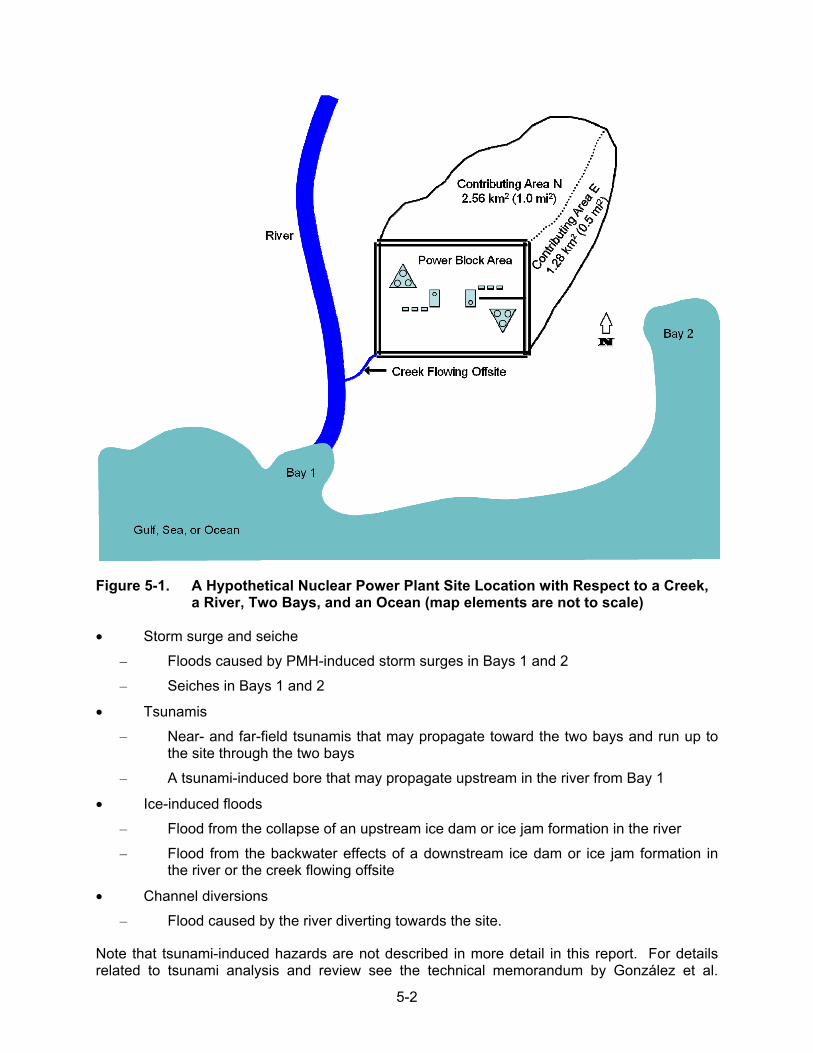
5-2
Figure 5-1. A Hypothetical Nuclear Power Plant Site Location with Respect to a Creek, a River, Two Bays, and an Ocean (map elements are not to scale)
• Storm surge and seiche
– Floods caused by PMH-induced storm surges in Bays 1 and 2
– Seiches in Bays 1 and 2
• Tsunamis
– Near- and far-field tsunamis that may propagate toward the two bays and run up to the site through the two bays
– A tsunami-induced bore that may propagate upstream in the river from Bay 1
• Ice-induced floods
– Flood from the collapse of an upstream ice dam or ice jam formation in the river
– Flood from the backwater effects of a downstream ice dam or ice jam formation in the river or the creek flowing offsite
• Channel diversions
– Flood caused by the river diverting towards the site.
Note that tsunami-induced hazards are not described in more detail in this report. For details related to tsunami analysis and review see the technical memorandum by González et al.
5-3
(2007) and the report by Prasad (2009). The remaining scenarios listed above should be described in sufficient detail and should include a review of historical flood occurrences and other pertinent site-specific data. These descriptions should be used to establish the relative importance of each of the flooding mechanisms at the site. For example, if the winters in the vicinity of the site are mild such that extensive ice formations for sustained periods do not occur and historical ice dam or ice jam formations have not been observed, flooding by ice-induced events could be ruled out. The remaining flooding mechanisms and respective plausible flood scenarios for each of these mechanisms constitute the set of alternative conceptual models for flooding at the site. These alternative conceptual models should then be analyzed further using the HHA approach described in Chapter 2. As described in Section 5.3 below, the selection of numerical flood-simulation models also depends on the set of plausible, site-specific, alternative conceptual models.
5.2 Quality Assurance Criteria for Simulation Models
After the selection of alternative conceptual models that may result in the design bases, the estimation of hazards is carried out. Frequently, simulation models are needed to estimate the flood hazards caused by hypothetical events such as the PMP, PMH, or dam breaches.
Appendix B of 10 CFR Part 50 requires that the safety-related SSCs of nuclear power plants prevent or mitigate the consequences of postulated accidents that could cause undue risk to public health and safety. The appendix also describes quality assurance requirements for design, manufacture, construction, and operations of these SSCs. Therefore, any flood-simulation models that are used to establish the design bases of safety-related SSCs must comply with the requirements of this appendix.
5.3 Selecting Simulation Models to Use
Under most circumstances, flood-simulation models developed by Federal agencies such as the USACE or academic and research institutions that are currently being used in standard engineering practice are adequate for estimation of hazards to safety-related SSCs at a nuclear power plant site. These models are used in engineering practice and have a history of validation and verification (e.g., USACE 2010).
However, there could be circumstances under which a customized flood-simulation model may be developed to account for site-specific conditions. A complete documentation of the technical bases of the customized model should be carried out. The documentation should include the following:
• a description of all components of the model
• a description of the governing equations
• a description of the model implementation details including, where appropriate, simplifying assumptions, spatial and temporal discretization schemes, interpolation methods, solution procedures, timesteps used, and convergence criteria
• a description of all model parameters
• input data requirements
• output details.

5-4
The numerical simulation models should be selected to ensure that the hydrodynamic conditions that are expected to occur at and near the site are adequately characterized by the model. The paragraphs below describe a few plausible scenarios where the site-specific hydrodynamic conditions may greatly influence the selection of appropriate simulation models. Notice that the plausible scenarios described below should already have been identified during the development of alternative conceptual models.
For example, for a cascading dam-breach event upstream of the site depicted in Figure 5-1 in which the river near the site is constrained by levees that are not designed to withstand the flood expected during the dam-breach event, it may be postulated that the levees would be overtopped by the dam-failure flood and water would flow through a breach in the levee toward the site. Under this scenario, a two-dimensional hydrodynamic model may need to be used because the flow is not constrained within the river channel anymore. At the same time, the flood may carry significant amounts of sediments from the levee material along with the flow. The sediment-laden water would have an increased density and therefore would cause increased drag forces on structures in its path. A sediment erosion and deposition model may need to be used to estimate the sediment concentrations near structures of interest.
Large floods generated by PMP events or multiple dam failures are also expected to overflow the banks of rivers and streams and occupy adjoining overbank and floodplain areas. Typically, overbank and floodplain areas contain vegetation and may also contain buildings and other structures. Because of the presence of these obstacles to flow, the overbank and floodplain areas have greater roughness than the main river channel. Therefore, an appropriate hydraulic model should be selected that allows roughness coefficients to vary along a channel cross-section.
Large floods are expected to generate a significantly greater flow velocity than a normal bankfull discharge. Therefore, it is plausible that these floods would result in significantly greater erosion of the banks and the channel bottom. The eroded material would be carried along with the flow. It is also plausible that the faster velocities of flow in the overbank or floodplain areas would result in debris being carried along with the flow. When the flow carrying the sediment and debris enters a downstream reservoir impounded by a dam, flow velocities would reduce and the sediment and debris may settle in the reservoir. Depending on the size of the downstream reservoir, the sedimentation may result in changes in the reservoir’s storage capacity and its stage-discharge characteristics. The model should account for these changes to simulate the flood dynamics downstream of the reservoir accurately.
In several regions of the United States, snowfall occurs during the winter and results in a snowpack at the beginning of spring. Rain-on-snow events have resulted in large floods in the past (Kattelmann et al. 1991; Kroczynski 2004; McCabe et al. 2007). Even a moderately severe rainfall event on an existing snowpack that is ready to start melting may cause severe flooding. The ANS (1992) recommends investigation of combined events consisting of a 100-year snow-season rainfall event on a probable maximum snowpack and a snow-season PMP on a 100-year snowpack as alternative scenarios for precipitation-caused flooding. A snowmelt model may be necessary to simulate the runoff. The USACE HEC-HMS contains snowmelt functionality and should be used to simulate rain-on-snow floods. The soils may be frozen during a rain-on-snow event, and therefore should be assumed to allow no infiltration.
5-5
5.4 Accounting for Uncertainty in Input and Model Parameters for Estimation of Design-Basis Flood Hazards
To estimate hazards caused by precipitation-generated floods at a site, usually two simulation models are needed. The first model is usually called a hydrologic model that requires hydrometeorological input and specification of a set of hydrologic model parameters that control the rainfall-runoff processes. The hydrologic model predicts the time history of discharges, called hydrographs, at several points of interest within the drainage basin upstream of the site. The second model, usually called a hydraulic model, requires a set of hydraulic model parameters and the hydrographs simulated by the hydrologic model as input. The hydraulic model predicts dynamic properties of the flood discharge such as velocity and depth.
Generally, the values of inputs to and parameters of flood simulation models contain uncertainty. The uncertainty in hydrometeorological inputs exists because they can only be measured with some degree of inherent error. Identification of model parameters is uncertain because it is based on imperfectly measured input and predicted variables. The model parameters also contain uncertainty because of simplification of the true, complete, and frequently unknown, governing equations, which results in the model being only an approximation of reality. Therefore, predictions from flood-simulation models also contain uncertainty.
Rainfall loss rates and rainfall-to-runoff transformation functions are the other two commonly used components in the hydrologic model. Loss rates specify the infiltration into soil. Because generally the hydrologic models used in standard engineering practice do not implement detailed characterization of groundwater flow into streams, the infiltrated water does not contribute to runoff generation. Therefore, specification of a non-zero loss rate reduces runoff generated from the PMP.
Rainfall-to-runoff transformation functions have been represented by unit hydrographs (Sherman 1932) in surface-water hydrology for quite some time. Unit hydrographs can be derived from observed rainfall and corresponding measured streamflow (Chow et al. 1988). The main characteristics of a unit hydrograph are as follows:
• a runoff volume equivalent to a unit depth over the drainage area
• a duration over which the rainfall excess occurs
• a constant time-to-peak and a constant time base.
The unit hydrograph approach assumes that the rainfall-runoff response of a drainage area is linear; i.e., the direct runoff hydrograph form a rainfall excess of a given amount can simply be obtained by multiplying the unit hydrograph ordinates by the rainfall excess. However, recent research indicates that the characteristics of unit hydrographs, including time-to-peak and the time base, may depend on rainfall intensity. Some of these issues are discussed in Appendix I.
To estimate unit hydrographs in ungauged drainage basins, several approaches have been developed (Chow et al. 1988). These approaches are based on observed data and generalizations that are assumed to be valid in other drainage basins. Therefore, the rainfall-runoff transformation function itself behaves as a model parameter that contains some uncertainty. In practice, unit hydrographs should be derived from rainfall and runoff measured in the drainage basin where the site is located. Also, because the characteristics of unit hydrographs depend on rainfall intensity, only large storms that generate extreme floods should be used in derivation of a unit hydrograph that would be used to estimate the PMF. Past studies (Pilgrim and Cordery, 1993; USACE 1994) have indicated that unit hydrographs
5-6
estimated for smaller storms should be adjusted to account for conditions that would be expected to occur during a PMP. These adjustments are also described in Appendix I.
The estimate of dynamic properties of the flood discharge using a hydraulic model (e.g., USACE HEC-RAS) depends on several model parameters, principally the roughness coefficient. For a given discharge, increased roughness of the channel impedes the flow and therefore results in slower flow velocity compared to a smoother channel of otherwise identical properties (e.g., slope and cross-section). Therefore, the flow of some discharge is conveyed at a larger depth and slower velocity in a rougher channel compared to that in a smoother channel. The hydrostatic and hydrodynamic loadings on SSCs depend on the depth of flow and the velocity of flow, respectively. It follows then, that the hydrostatic loading is maximized by increasing depths of flow, which may result from increased roughness of the channel, and the hydrodynamic loading is maximized by reducing the roughness. Also, the duration of inundation may be greater for slower flow and therefore would result in a longer time of exposure to the flood hazards. Therefore, in estimation of design-basis loadings from floods, the roughness coefficient should be selected carefully to account for the tradeoffs described above.
Design-basis flood analysis should carefully describe and quantify the sources of uncertainty by appropriately selected sensitivity analyses. The design-basis flood hazards should then be selected carefully from the predicted range of values of these hazard metrics (e.g., depth of flow, density of flow, velocity of flow, and duration of inundation) to ensure that the most adverse conditions are accounted for.
5.5 Validation
The accuracy of the model should be validated using site-specific data. Because the floods used to estimate the design bases are usually hypothetical and extreme, care should be exercised to ensure that the validation process accounts for the extreme severity of the recommended hydrometeorological events and conditions. The validation details should include the following:
• a description of the validation approach
• all validation datasets used including site-specific data
• a demonstration that the validation of the simulation model includes floods approaching the severity of those resulting from recommended hydrometeorological events and conditions.
It is extremely important that the validation of the simulation models and associated parameters use the largest reported historical floods near the site. The ability of the models to reproduce historical floods provides some assurance that the estimated design-basis floods near the site would not be underestimated.
5.6 Reconciling Deterministic and Probabilistic Notions in the Context of Design-Basis Flood Estimation
The primary focus of this report is to describe deterministic approaches for the estimation of design-basis flood events. The cause of the flood is assumed to be a worst-case event that cannot be exceeded in terms of severity; however, at the same time, the PMF is defined to be the most severe, reasonably possible flood at a site and the PMH is defined as the most severe hurricane that can reasonably occur in a region. There is some ambiguity in these definitions that introduces subjectivity in the selection of these events. Additional subjectivity is also
5-7
introduced in the estimation of design-basis floods during selection of model parameters and antecedent conditions. Several studies have criticized the “probable maximum” concept, especially that of the PMP (Benson 1973; Kite 1988; Dingman 1994).
The SSCs exposed to flood hazards should be designed to prevent plant flooding risk beyond the Commission safety goals. The estimation of a deterministic design-basis flood does not specify its probability-of-exceedance. In general terms, “probable maximum” events are thought to have “virtually no risk of exceedance” (ANS 1992) and combining the effects of coincident events provides an additional margin of safety. Some efforts have focused on the estimation of the probability-of-exceedance of “probable maximum” events (Hershfield 1961, 1965; Newton 1983; Nobilis et al. 1991; Koutsoyiannis 1999; Papalexiou and Koutsoyiannis 2006). The Hershfield (1961, 1965) method is a statistical approach and is adopted by the World Meteorological Organization (WMO 1986). The ANS (1992) recommended that an average annual probability-of-exceedance less than 10-6 is an acceptable goal for selection of flood design bases.
Chery and Wescott (1985) summarized the studies of Hershfield (1961) and Newton (1983) in a report to the Advisory Committee on Reactor Safeguards (ACRS) subcommittees on Reactor Radiological Effects and Extreme External Phenomena. They concluded that the mean probability of occurrence of a PMF is less than 10-5. They were not able to determine the confidence limits on the mean probability of occurrence of the PMF.
Nobilis et al. (1991) used annual maximum daily precipitation from 504 stations in Austria to estimate the PMP using the method of Hershfield (1961, 1965), but obtained estimates of PMP that were smaller than observed extreme precipitation. Nobilis et al. (1991) concluded that the estimated PMP values were based on the Hershfield frequency factor estimated from average of mean extreme precipitation values and therefore did not adequately represent “outliers.”
Koutsoyiannis (1999) presented a reanalysis of Hershfield’s data. He determined that there was no upper limit to Hershfield’s frequency factor, which is the basis for estimating the PMP (WMO 1986). Therefore, Koutsoyiannis (1999) concluded that there is no upper limit to the amount of precipitation. He proposed to use a statistical analysis of all frequency factors representing annual maximum rainfalls at different stations rather than the analysis of only the frequency factor corresponding to the maximum observed rainfall at a station. Based on this modified analysis that used the generalized extreme value distribution, Koutsoyiannis (1999) was able to estimate that the Hershfield frequency factor of 15, used for estimating the PMP, corresponds to a return period of approximately 60,000 years. He recommended that the concept of PMP should be substituted with the determination of a design rainfall estimated for a selected probability-of-exceedance.
Papalexiou and Koutsoyiannis (2006) concluded that an upper bound to dew point, an assumption also used in the deterministic storm maximization and transposition approaches to the estimation of the PMP, does not exist.
Fontaine and Potter (1989) described stochastic storm transposition, a generalization to the transposition method used to estimate PMP. The generalization was based on the assumption that a storm of a given magnitude occurring at a given location within a meteorologically homogeneous region could occur anywhere else within the region with the same probability with appropriate adjustments to its characteristics. The assumption effectively provides a regional and larger set of extreme storms from which frequency distribution of extreme storms for a location of interest could be estimated. Wilson and Foufoula-Georgiou (1990) applied a similar method to the midwestern United States, but noted a need for further research.

5-8
Douglas and Barros (2003) used a multifractal approach to estimate fractal maximum precipitation in the eastern United States. They describe the behavior of rainfall as a multiscaling cascade in which progressively higher intensity cells are embedded as the spatial scale decreases from synoptic to mesoscale to local. They estimated the 3-day fractal maximum and the 3-day 10-6 exceedance-probability design PMP using 327 daily and 1400 monthly time series data spanning from 1950 to 1997. Their estimates of the 3-day fractal maximum precipitation were consistently lower at 5 of the 7 locations, typically 50 to 70 percent of the 3-day PMP estimated using HMR 51 and 52. On the other hand, their estimates of the 3-day 10-6 exceedance-probability design PMP were consistently higher at 5 of the 7 locations, ranging from 122 to 200 percent of the 3-day PMP estimated using HMR 51 and 52. Douglas and Barros (2003) concluded that because the 3-day 10-6 exceedance-probability design PMP generally exceeds the HMR 51 and 52 estimates, it can be viewed as an upper bound of known risk.
The National Research Council (1988) study on estimation of probabilities of extreme floods also recommended the use of probabilistic methods for estimation of a range of floods and their associated probabilities rather than to focus on a single, large flood that was construed to represent an upper bound. The study mentioned two probabilistic approaches for determination of extreme floods at the site of interest: a statistical analysis of streamflow data and a statistical analysis of meteorological data coupled to a numerical model to simulate the physical processes involved in runoff generation. The study also recognized that the estimation of probability-of-exceedance of extreme floods would require extrapolation beyond the range of available observation. The study recommended three principles for improving extreme flood estimates: substituting space for time (regionalization), using structured models (spatial and inter-parametric dependences), and focusing on extreme value analysis (tails of distributions).
The National Research Council (1988) recommended several parametric statistical distributions including log-Pearson Type III, the generalized extreme value distribution, and Wakeby distribution. The study also mentions that nonparametric methods may also be suitable for analysis of extreme values.
The National Research Council (1988) recommended use of runoff simulation models in conjunction with the estimated magnitude and frequency of extreme meteorological events (such as those described above) to derive the probability-of-exceedance of extremely rare floods. The study noted that these models are capable of estimating complete hydrographs that can be very useful in design. It also noted that an appropriately chosen runoff model should be capable of simulating physical processes that are expected to occur during the very large events. The study mentioned that a study of extreme value events requires an explicit consideration of uncertainty that arises from sampling uncertainty, measurement errors, and modeling assumptions.
A comprehensive Probabilistic Flood Hazard Assessment (PFHA) methodology has not yet been developed. However, discrete components of the PFHA are now available, although the overall framework still needs to be developed. This report is not a suitable place to describe and develop these concepts. Only a brief mention of the overall approach is made. The following discussion is based on a hybrid approach similar to that recommended by the National Research Council (1988) where a numerical runoff simulation model is used in conjunction with the probabilistic representation of the statistical distribution of extreme meteorological events.
The PFHA consists of two discrete components:
1. probability distributions of meteorological input variables (such as precipitation, air temperature, relative humidity) of extreme events
5-9
2. derivation of probability distribution of flood hazards (such as discharge, flow depth and velocity, duration of inundation) using a numerical runoff simulation model or combination of models.
The probabilistic approaches for estimation of extreme value distributions have been in existence for some time. Both parametric and nonparametric approaches are now sufficiently well understood that they can be applied in practice. Data for estimation of extreme value distributions of meteorological variables often approach and exceed 100 years in the United States. Based on the recommendations of the National Research Council (1988), it should be relatively straightforward to accomplish component 1 above.
The derivation of probability distribution of flood hazards would require simulation of a large number of scenarios consisting of input datasets sampled from the joint probability distribution of the meteorological variables. One complicating factor in component 2 above is the need to account for uncertainty in model parameters that can also be represented as a joint probability distribution. Adaptive techniques for sampling have been developed (Freer et al. 1996; Kuczera and Parent 1998; Bates and Campbell 2001; Hossain and Anagnostou 2005) that can be used to minimize the number of simulated scenarios while providing adequate sampling of the parameter hyperspace. Schaefer and Barker (2002), Swain et al. (2004), and the USACE (2005) provide examples of some such implementations.
An integrated framework that establishes guidelines for bringing together already existing tools is needed to fully develop the PFHA approach. Further development of the PFHA approach is recommended for future study.
5.7 Effects of Climate Variability on Design-Basis Flood Estimation
Future changes in the hydrometeorological characteristics of the drainage basin upstream of a site can change precipitation-generated extreme floods at the site. Future changes in land use, increasing sedimentation of existing reservoirs, development of additional water and flood-control structures, and operational characteristics of existing controls can change the floods generated by dam breaches upstream of the site. Future changes in atmospheric, climatic, and oceanic conditions can change the characteristics of hurricanes and storm surges near a site.
Most of the debate related to long-term climate change is based on the argument that the global surface temperature is increasing at an accelerated rate over the last few decades (IPCC 2007a). The Intergovernmental Panel on Climate Change (IPCC) defines climate change as a change in the state of the climate that can be identified by detecting changes in the mean and/or the variability of its properties that persists for an extended period, typically decades or longer. The IPCC’s definition of climate change includes changes because of both natural variability and human activity.
The IPCC (2007a) reported that the linear warming trend in air temperature over 1956 to 2005 is 1.3 ºC—nearly twice that for 1906 to 2005, 0.74 ºC. The temperature increase is reported to be greater for the higher northern latitudes, average arctic temperatures are reported to have increased almost twice of the global average rate, and land surfaces are reported to have warmed faster than oceans.
The IPCC (2007a) reported that global average sea level rose at an average rate of approximately 1.8 mm per year from 1961 to 2003, while the rate was approximately 3.1 mm per year from 1993 to 2003. The study was not able to clearly conclude whether the increased rate of sea level rise over the latter period was because of decadal variability or because of an
5-10
increase in long-term trend. The IPCC (2007a) reported that 57 percent of the sea-level rise since 1993 is attributable to thermal expansion, 28 percent is attributable to decreases in glaciers and ice caps, and the remainder is attributable to losses from polar ice sheets.
The IPCC (2007a) reported that mountain glaciers and snow cover have declined all over the globe; the maximum area of seasonally frozen ground has decreased by approximately 7 percent in the Northern Hemisphere since 1900. The decrease of seasonally frozen ground is greater in spring, approximately 15 percent. The IPCC (2007a) also reported that since 1980, the surface temperature of the top of the permafrost has increased by approximately 3 ºC.
The IPCC (2007a) reported that precipitation has significantly increased in eastern North America. The study also reported that changes in the frequency of extreme weather events over the last five decades indicate that it is very likely that cold days, cold nights, and frosts have become less frequent over land areas; it is likely that heat waves have become more frequent over land areas; it is likely that the frequency of heavy precipitation events has increased; and it is likely that occurrences of extreme high sea levels have increased. The IPCC (2007a) also reported that since 1970, intense tropical cyclone activity in the North Atlantic has increased. During 1995 to 2004, 13.6 tropical storms, 7.8 hurricanes, and 3.8 major hurricanes occurred on an average compared to the 1970 to 1994 period, when the corresponding numbers were 8.6, 5, and 1.5, respectively (IPCC 2007b).
The IPCC (2007a) concluded with high confidence that changes in the hydrological systems include increased runoff and earlier spring peak discharge in glacier and snow-fed rivers and warming of lakes and rivers with associated effects on their thermal structure and water quality.
With respect to estimation of design-basis floods at nuclear power plant sites, the following changes reported by IPCC (2007a) are of importance:
• increases in surface temperature and precipitation
• decrease in snow cover and earlier spring peak runoff
• increase in intense cyclone activity
• increase in sea level.
It is not clear how extreme precipitation, such as the PMP, would change under an altered climate that is characterized by increased temperature and precipitation. Generally, however, increased temperatures may lead to an increase in precipitable water and therefore may increase the PMP amount. The changes in temperature and snow cover may also affect the way storm systems develop, change the time of year when they occur, and the paths they follow to the site. We are not aware of any studies that investigate these factors. Therefore, a sensitivity analysis that incorporates temperature and precipitation trends projected by the IPCC reports should be carried out to determine whether the site has adequate margins available to accommodate anticipated changes in the design-basis flood over the operational life of the plant.
Similarly, long-term increase in cyclonic activity has not been investigated to determine whether the PMH characteristics such as central pressure difference, size of the storm, track speed, and direction of approach may be affected in the altered climate scenarios. The estimates of PMH parameters may be subjected to a sensitivity analysis along with the accounting of projected sea-level rise during the operational life of the plant to determine whether the site has adequate margins available to accommodate anticipated changes in the design-basis flood. These sensitivity studies should be used for informed decision-making regarding selection of design bases and the need for protective structures and emergency procedures.
6-1
6 FUTURE DIRECTIONS
The estimation of design-basis floods at nuclear power plant sites is currently based on a set of deterministic approaches that specify the “probable maximum” flood precursor event. Hydrologic, hydraulic, thermal, and hydrodynamic models are currently used to predict a set of extreme candidate floods at the site from which the most severe design-basis flood hazards are selected. The guidance for estimation of some of the “probable maximum” flood precursor events was developed several decades ago and therefore is based on old and outdated datasets. For example, various HMRs were prepared in the 1970s and 1980s (Schreiner and Riedel 1978; Hansen et al. 1982) and therefore have not used extreme precipitation data recorded since their publication. The current guidance for estimation of PMH was published in 1979 and has not been updated to include more recent data.
Future efforts to improve the reliability of the design-basis flood estimate should include the following:
1. Incorporation of more recent site-specific hydrometeorological datasets in the estimation of design-basis floods. It should be noted here that an applicant can most reasonably use these datasets at its site for validation that the estimated design-basis flood is appropriately conservative, identification of site-specific model parameters, and demonstration of existence of sufficient margin in site characteristics and selected design bases.
2. Development of probabilistic approaches for estimation of design-basis flood. An outline of the PFHA is described in Chapter 5. A probabilistic approach has the inherent advantage of clearly articulating the level of risk that a selected design basis would likely encounter during the operational life of the plant. A hybrid approach that uses simulation models and explicitly accounts for various uncertainties in estimation of extreme floods, augmented by probabilistic assessment of the level of risk to which safety-related SSCs would be exposed should be developed.
3. Development of high-resolution hydrometeorological datasets. The recent availability of high-resolution data such as terrain and bathymetry data, subbasin delineations, channel network and its connectivity, more reliable and dense meteorological data, remotely sensed imagery, and spatial datasets representing soil and vegetation has greatly improved parameterization of numerical models. Future advances in data collection, verification, archiving, and dissemination would increase the reliability of model formulation and also increase the opportunities to validate model predictions. Future guidance for estimation of design-basis floods should take advantage of these improvements in data availability and reliability to demonstrate that public health and safety criteria of the NRC’s regulations are clearly met at all sites.
4. Guidance related to climate variability and global climate change. Recent developments in global climate change research has shown that significant effects at global and national scales are expected (IPCC 2007a, b). However, the effects of these changes at the drainage basin- and site-scale need site-specific analysis. It is also unclear how changing climate affects the “probable maximum” events that are used for design-basis flood estimation at nuclear power plant sites. The characteristic scales of “probable maximum” events vary significantly (local intense precipitation is a site-scale phenomenon, PMP and PMF are drainage basin- to regional-scale phenomena, and PMH could be affected by changes at intercontinental scales).

7-1
7 REFERENCES
10 CFR Part 50. Code of Federal Regulations, Title 10, Energy, Part 50, “Domestic Licensing of Production and Utilization Facilities.”
10 CFR Part 52. Code of Federal Regulations, Title 10, Energy, Part 52, “Licenses, Certifications, and Approvals for Nuclear Power Plants.”
Adamowski K. 1985. “Nonparametric Kernel Estimation of Flood Frequencies.” Water Resources Research 21(11):1585-1590.
American Nuclear Society (ANS). 1992. American National Standard for Determining Design Basis Flooding at Power Reactor Sites. Prepared by the American Nuclear Society Standards Committee Working Group ANS-2.8, La Grange Park, Illinois.
American Society of Mechanical Engineers (ASME). 2009. “Addenda to ASME/ANS RA-S–2008.” Standard for Level 1/Large Early Release Frequency Probabilistic Risk Assessment for Nuclear Power Plant Applications. ASME/ANS RA-Sa–2009, New York.
Benson M.A. 1973. “Thoughts on the design of design floods.” In the Proceedings of the 2nd International Symposium in Hydrology, at Fort Collins, Colorado. Water Resources Publications, Fort Collins, Colorado. Pp.27-33.
BOSS International. 1988. “BOSS HMR52 Users Manual.” BOSS International, Inc., Madison, Wisconsin.
Brunner G. and M. Gee. 2009. “Extreme Flood Risk Methods.” In the Proceedings of the Association of State Dam Safety Officials Annual Conference. Lexington, Kentucky.
Bunya S, J. Westerink, J.C. Dietrich, H.J. Westerink, L.G. Westerink, J. Atkinson, B. Ebersole, J.M. Smith, D. Resio, D., R. Jensen, M.A. Cialone, R. Luettich, C. Dawson, H.J. Roberts, and J. Ratcliff. 2010. “A High Resolution Coupled Riverine Flow, Tide, Wind, Wind Wave and Storm Surge Model for Southern Louisiana and Mississippi: Part I–Model Development and Validation.” Monthly Weather Review 138:345-377.
Chow V.T. 1959. Open-Channel Hydraulics. McGraw-Hill Book Company, New York.
Chow V.T., D.R. Maidment, and L.W. Mays. 1988. Applied Hydrology. McGraw-Hill Book Company, New York.
Clark C.O. 1945. “Storage and the Unit Hydrograph.” Transactions of the American Society of Civil Engineers 110:1419-1488.
Cudworth A.G. Jr. 1989. “Flood Hydrology Manual.” A Water Resources Technical Publication, U.S. Department of Interior, Bureau of Reclamation, Denver, Colorado.
Dingman S. L. 1994. “Physical Hydrology.” 1st edition. Prentice Hall, Inc., Upper Saddle River, New Jersey.
Doten C.O., L.C. Bowling, E.P. Maurer, J.S. Lanini, and D.P. Lettenmaier. 2006. “A spatially distributed model for the dynamic prediction of sediment erosion and transport in mountainous forested watersheds.” Water Resources Research 42(4) doi: W0441710.1029/2004WR003829.
7-2
Douglas E.M. and A.P. Barros. 2003. “Probable maximum precipitation estimation using multifractals: Application in the eastern United States.” Journal of Hydrometerology 4: 1012-1024.
England J.F. Jr., R.D. Jarrett, and J.D. Salas. 2003. “Data-based comparisons of moments estimators that use historical and paleoflood data.” Journal of Hydrology 278(1-4):170-194.
Federal Emergency Management Agency. 2010. “Numerical Models Meeting the Minimum Requirement of National Flood Insurance Program.” Available at http://www.fema.gov/plan/prevent/fhm/en_coast.shtm. Accessed December 20, 2010.
Federal Energy Regulatory Commission. 2001. Engineering Guidelines for the Evaluation of Hydropower Projects. Chapter 8 – “Determination of the Probable Maximum Flood.” Washington, D.C.
Flynn K.M., W.H. Kirby, and P.R. Hummel. 2006. “Users Manual for Program PeakFQ, Annual Flood-Frequency Analysis Using Bulletin 17B Guidelines.” In Chapter 4, Section B of the U.S. Geological Survey Techniques and Methods Report Book 4, U.S. Geological Survey, Reston, Virginia.
Fontaine T.A. and K.W. Potter. 1989. “Estimating probabilities of extreme rainfalls.” Journal of Hydraulic Engineering 115(11):1562-1575.
González F.I., E. Bernard, P. Dunbar, E. Geist, B. Jaffe, U. Kânŏglu, J. Locat, H. Mofjeld, A. Moore, C. Synolakis, V. Titov, and R. Weiss (Science Review Working Group). 2007. “Scientific and technical issues in tsunami hazard assessment of nuclear power plant sites.” NOAA Technical Memorandum OAR PMEL-136, Pacific Marine Environmental Laboratory, Seattle, Washington.
Griffis V.W. and J.R. Stedinger. 2007. “Evolution of Flood Frequency Analysis with Bulletin 17.” Journal of Hydrologic Engineering 12(3):283-297.
Gupta V.K., E. Waymire, and C.T. Wang. 1980. “A representation of an instantaneous unit hydrograph from geomorphology.” Water Resources Research 16(5):855-862.
Haan C.T. 1977. Statistical Methods in Hydrology. The Iowa State Press, Ames, Iowa.
Hansen E.M., L.C. Schreiner, and J.F. Miller. 1982. Application of Probable Maximum Precipitation Estimates – United States East of the 105th Meridian. NOAA Hydrometeorological Report 52, National Weather Service, Washington, D.C.
Hershfield D.M. 1961. “Rainfall Frequency Atlas of the United States for Durations from 30 Minutes to 24 Hours and Return Periods from 1 to 100 Years.” Technical Paper No. 40, U.S. Weather Bureau, U.S. Department of Commerce, Washington, D.C.
Hershfield D.M. 1965. “Method for Estimating Maximum Probable Precipitation.” Journal of American Waterworks Association 57:965-972.
Holland G.J. 1980. “An analytic model of the wind and pressure profiles in hurricanes.” Monthly Weather Review108:1212-1218.
7-3
Interagency Advisory Committee on Water Data (IACWD). 1982. “Guidelines for determining flood flow frequency.” Bulletin 17B of the Hydrology Subcommittee, Office of Water Data Coordination, U.S. Geological Survey, Reston, Virginia.
International Atomic Energy Agency (IAEA). 2003. Flood Hazard for Nuclear Power Plants on Coastal and River Sites. IAEA Safety Guide No. NS-G-3.5, Vienna, Austria.
Intergovernmental Panel on Climate Change (IPCC). 2007a. Climate Change 2007: Synthesis Report. Core Writing Team, RK Pachauri and A. Reisinger (eds.), Geneva, Switzerland.
Intergovernmental Panel on Climate Change (IPCC). 2007b. Climate Change 2007: The Physical Science Basis. S. Solomon, D. Qin, M. Manning, Z. Chen, M. Marquis, K.B. Averyt, M. Tignor, and H.L. Miller (eds.). Cambridge University Press, Cambridge, United Kingdom and New York..
Irish J.L., D.T. Resio, and J.J. Ratcliff. 2008. “The influence of storm size on hurricane Surge.” Journal of Physical Oceanography 38(11):2003-2013.
Irish J.L., D.T. Resio, and M.A. Cialone. 2009. “A surge response function approach to coastal hazard assessment. Part 2: Quantification of spatial attributes of response functions.” Natural Hazards 51(1):183-205.
Jelesnianski C.P., J. Chen, and W.A. Shaffer. 1992. SLOSH: Sea, Lake, and Overland Surges from Hurricanes. NOAA Technical Report NWS 48, National Oceanic and Atmospheric Administration National Weather Service, Silver Spring, Maryland.
Kattelmann R., N. Berg, and B. McGurk. 1991. “A history of rain-on-snow floods in the Sierra Nevada.” Proceedings of the Western Snow Conference 59:138-141.
Kite G.W. 1988. “Frequency and Risk Analysis in Hydrology.” Water Resources Publications, Littleton, Colorado.
Koutsoyiannis D. 1999. “A probabilistic view of Hershfield’s method for estimating probable maximum precipitation.” Water Resources Research 35(4):1313-1322.
Kroczynski S. 2004. “A Comparison of Two Rain-on-Snow events and the Subsequent Hydrologic Response in Three Small River Basins in Central Pennsylvania.” Eastern Region Technical Attachment 2004-04, National Oceanic and Atmospheric Administration National Weather Service Eastern Region Publications, Bohemia, New York.
Lall U., Y. Moon, and K. Bosworth. 1993. “Kernel Flood Frequency Estimators: Bandwidth Selection and Kernel Choice.” Water Resources Research 29(4):1003-1015.
McCabe, G.J., M.P. Clark, and L.E. Hay. 2007. “Rain-on-snow events in the Western United States.” Bulletin of the American Meteorological Society 88(3):319-328.
Mukai A.Y., J.J. Westerink, R.A. Luettich, Jr., and D. Mark. 2002. Eastcoast 2001, A Tidal Constituent Database for Western North Atlantic, Gulf of Mexico, and Caribbean Sea. Coastal and Hydraulics Laboratory, U.S. Army Corps of Engineers, Vicksburg, Mississippi.
Nash J.E. 1960. “A Unit Hydrograph Study with Particular Reference to British Catchments.” Proceedings of the Institute of Civil Engineers 17:249-282.

7-4
National Research Council. 1988. Estimating Probabilities of Extreme Floods, Methods and Recommended Research. Committee on Techniques for Estimating Probabilities of Extreme Floods, National Academy Press, Washington, D.C.
Natural Resources Conservation Service (previously the U.S. Soil Conservation Service). 1985. “Hydrology.” Section 4 in National Engineering Handbook.” U.S. Department of Agriculture, Washington, D.C.
Newton, D. 1983. “Realistic Assessment of Maximum Flood Potential.” Proceedings of the American Society of Civil Engineers, Journal of the Hydraulics Division 109:905-918.
Nobilis, F., T. Haiden, and M. Kerschbaum. 1991. “Statistical Considerations Concerning Probable Maximum Precipitation (PMP) in the Alpine Country of Austria.” Theoretical and Applied Climatology 44:89-94.
O’Connell D.R.H., D.A. Ostenaa, D.R. Levish, and R.E. Klinger. 2002. “Bayesian flood frequency analysis with paleohydrologic bound data.” Water Resources Research 38(5), 1058, doi: 10.1029/2000WR000028.
Papalexiou S.M. and D. Koutsoyiannis. 2006. “A probabilistic approach to the concept of Probable Maximum Precipitation.” Advances in Geosciences 7:51-54.
Pilgrim D.H. and I. Cordery. 1993. “Flood Runoff.” Chapter 9 in Handbook of Hydrology, D.R. Maidment (ed.), McGraw-Hill Book Company, New York.
Powell M.D., P.J. Vickery, and T.A. Reinhold. 2003. “Reduced drag coefficient for high wind speeds in tropical cyclones.” Nature 203:279-283.
Prasad R. 2009. Tsunami Hazard Assessment at Nuclear Power Plant Sites in the United States of America. NUREG/CR-6966, Office of New Reactors, U.S. Nuclear Regulatory Commission, Washington, D.C.
Resio D.T., J.L. Irish, and M.A. Cialone. 2009. “A surge response function approach to coastal hazard assessment: Part 1, Basic Concepts.” Natural Hazards 51(1):163-182.
Rodriguez-Iturbe I. and J.B. Valdes. 1979. “The geomorphologic structure of hydrologic response.” Water Resources Research 15(6):1409-1420.
Rodriguez-Iturbe I. and A. Rinaldo. 1997. Fractal River Basins: Chance and Self-Organization. Cambridge University Press, New York.
Schaefer M.G. and B.L. Barker. 2002. “Stochastic Event Flood Model.” Chapter 20 in Mathematical Models of Small Watershed Hydrology and Applications, V.P. Singh and D. Frevert (eds.), Water Resources Publications, Littleton, Colorado, p. 707-748.
Scheffner N.W. 2008. “Water Levels and Long Waves.” In: Demirbilek, Z., Coastal Engineering Manual, Part II, Coastal Hydrodynamics Chapter 5-6 , Engineer Manual 1110-2-1100, U.S. Army Corps of Engineers, Washington, D.C..
Schreiner L.C. and J.T. Riedel. 1978. Probable Maximum Precipitation Estimates, United States East of the 105th Meridian. Hydrometeorological Report No. 51, U.S. Department of Commerce, National Oceanic and Atmospheric Administration, and U.S. Department of Army Corps of Engineers, Washington, D.C.
7-5
Schwerdt R.W., F.P. Ho, and R.R. Watkins. 1979. Meteorological Criteria for Standard Project Hurricane and Probable Maximum Hurricane Windfields, Gulf and East Coasts of the United States. NOAA Technical Report NWS 23, National Oceanic and Atmospheric Administration, National Weather Service, Silver Spring, Maryland.
Sherman L.K. 1932. “Streamflow from Rainfall by the Unit-graph Method.” Engineering News Record 108:501–505.
Simpson R.H. and H.Riehl. 1981. The Hurricane and Its Impact. Louisiana State University Press, Baton Rouge.
Snyder F.F. 1938. “Synthetic Unit-Graphs.” Transactions of the American Geophysical Union 19(1938):447-454,.
Stedinger J.R., R.M. Vogel, and E. Foufoula-Georgiou. 1993. “Frequency Analysis of Extreme Events.” Chapter 18 in Handbook of Hydrology, D.R. Maidment (ed.), McGraw-Hill Book Company, New York.
Stevens C.L. and G.A. Lawrence. 1997. “Estimation of wind-forced internal seiche amplitudes in lakes and reservoirs, with data from British Columbia, Canada.” Aquatic Sciences 59(2):115-134.
Swain R.E., J.F. England, Jr., K.L. Bullard, and D.A. Raff. 2006. “Guidelines for Evaluating Hydrologic Hazards.” U.S. Department of Interior, Bureau of Reclamation, Denver, Colorado.
Swain R.E., J.F. England, Jr., K.L. Bullard, and D.A. Raff. 2004. Hydrologic Hazard Curve Estimating Procedures. Dam Safety Research Program Research Report DSO-04-08, U.S. Department of Interior, Bureau of Reclamation, Denver, Colorado.
U.S. Army Corps of Engineers (USACE). 2010. “Hydrologic Modeling System (HEC-HMS) Validation Guide, Version 3.5.” Available at http://www.hec.usace.army.mil/software/hec-hms/. Accessed December 20, 2010, 2010.
U.S. Army Corps of Engineers (USACE). 2009a. “Engineer Regulations and Manuals.” Publications of the U.S. Army Corps of Engineers. Washington, D.C.
U.S. Army Corps of Engineers (USACE). 2009b. “Hydrologic Modeling System (HEC-HMS).” Available at http://www.hec.usace.army.mil/software/hec-hms/. Accessed June 9, 2009, 2009c.
U.S. Army Corps of Engineers (USACE). 2009c “River Analysis System (HEC-RAS).” Available at http://www.hec.usace.army.mil/software/hec-ras/. Accessed June 10, 2009, 2009d.
U.S. Army Corps of Engineers (USACE). 2008a. HEC-RAS River Analysis System User’s Manual. Version 4.0. U.S. Army Corps of Engineers Hydrologic Engineering Center, Davis, California. Available at http://www.hec.usace.army.mil/software/hec-ras/documents/HEC-RAS_4.0_Users_Manual.pdf. Accessed June 10, 2009.
U.S. Army Corps of Engineers (USACE). 2008b. “Hydrologic Modeling System HEC-HMS User’s Manual. Version 3.3.” U.S. Army Corps of Engineers Hydrologic Engineering Center, Davis, California. Available at http://www.hec.usace.army.mil/software/hec-hms/documentation/HEC-HMS_Users_Manual_3.3.pdf. Accessed June 9, 2009.
7-6
U.S. Army Corps of Engineers (USACE). 2008c. Inflow Flood Hydrographs. USACE Dam Safety Program Portfolio Risk Assessment Draft Report, Washington D.C.
U.S. Army Corps of Engineers (USACE). 2005. Stochastic Modeling of Extreme Floods on the American River at Folsom Dam. Flood-Frequency Curve Extension. Research Document 48, Institute for Water Resources, Hydrologic Engineering Center, Davis, California.
U.S. Army Corps of Engineers (USACE). 1997. Hydrologic Engineering Requirements for Reservoirs. Engineer Manual 1110-2-1420, Washington, D.C.
U.S. Army Corps of Engineers (USACE). 1994. Flood-Runoff Analysis. Engineer Manual 1110-2-1417, Washington, D.C..
U.S. Army Corps of Engineers (USACE). 1991. “Inflow design floods for dams and reservoirs.” Engineer Regulation 1110-8-2(FR), Washington, D.C.
U.S. Department of Interior, Bureau of Reclamation (Reclamation). 2010. Best Practices in Dam Safety Risk Analysis, Version 2.1. Denver, Colorado.
U.S. Department of Interior, Bureau of Reclamation (Reclamation). 2003. Guidelines for Achieving Public Protection in Dam Safety Decision-Making. Denver, Colorado.
U.S. Department of Interior, Bureau of Reclamation (Reclamation). 2002. “Interim Guidelines for Addressing the Risk of Extreme Hydrologic Events.” Denver, Colorado.
U.S. Department of Interior, Bureau of Reclamation (Reclamation). 1987. Design of Small Dams. Third Edition. A Water Resources Technical Publication, Washington, D.C.
U.S. Department of Interior, Bureau of Reclamation (Reclamation). 1977. Design of Arch Dams. A Water Resources Technical Publication, Denver, Colorado.
U.S. Department of Interior, Bureau of Reclamation (Reclamation). 1976. Design of Gravity Dams. A Water Resources Technical Publication, Denver, Colorado.
U.S. Department of Energy (DOE). 2002. Natural Phenomena Hazards Design and Evaluation Criteria for Department of Energy Facilities. DOE Standard STD-1020-2002, Washington, D.C.
U.S. Department of Energy (DOE). 1995 Natural Phenomena Hazards Assessment Criteria. DOE Standard STD-1023-95, Washington, D.C..
U.S. Nuclear Regulatory Commission (NRC). 2007a. A Performance-Based Approach to Define the Site-Specific Earthquake Ground Motion. Regulatory Guide 1.208, Washington, D.C.
U.S. Nuclear Regulatory Commission (NRC). 2007b. Seismic Design Classification. Regulatory Guide 1.29, Rev. 4, Washington, D.C.
U.S. Nuclear Regulatory Commission (NRC). 1977. Design Basis Flood for Nuclear Power Plants. Regulatory Guide 1.59, Rev. 2, Washington, D.C.
U.S. Nuclear Regulatory Commission (NRC). 1976. Flood Protection for Nuclear Power Plants. Regulatory Guide 1.102, Rev. 1, Washington, D.C.
7-7
Westerink J.J., R.A. Luettich, J.C. Feyen, J.H. Atkinson, C. Dawson, H.J. Roberts, M.D. Powell, J.D. Dunion, E,J, Kubatko, H. and Pourtaheri. 2008. “A basin to channel scale unstructured grid hurricane storm surge model applied to southern Louisiana.” Monthly Weather Review136(3):833–864.
Wigmosta M.S., B. Nijssen, P. Storck, and D.P. Lettenmaier. 2002. “The Distributed Hydrology Soil Vegetation Model.” In Mathematical Models of Small Watershed Hydrology and Applications, V.P. Singh, D.K. Frevert (eds.), p. 7-42, Water Resource Publications, Littleton, Colorado. .
Wigmosta M.S., L. Vail, and D.P. Lettenmaier. 1994. “A distributed hydrology-vegetation model for complex terrain.” Water Resources Research30:1665-1679.
Wilson L.L. and E. Foufoula-Georgiou. 1990. “Regional Rainfall Frequency Analysis via Stochastic Storm Transposition.” Journal of Hydraulic Engineering 116(7):859-880.
World Meteorological Organization (WMO). 1986. “Manual for Estimation of Probable Maximum Precipitation.” Second edition, WMO No. 332, Operational Hydrology Report No. 1, Geneva, Switzerland.
Wüest A. and D.M. Farmer. 2003. “Seiche.” In McGraw-Hill Encyclopedia of Science and Technology, 9th Edition, McGraw-Hill Companies, New York.

8-1
8 GLOSSARY
alternative conceptual models the set of conceptualizations that describes how plausible hydrometeorological phenomena may result in flood events that can cause hazards at a site; the set should account for uncertainty in geohydrologic, hydraulic, geoseismic, meteorologic, and structural characteristics that are relevant for the plausible phenomena.
antecedent precipitation a precipitation event that precedes the main and usually larger storm
causative Mechanism hydrometeorological phenomenon that may cause a flood
Code of Federal Regulations (CFR) a collection of general and permanent rules published by executive departments and agencies of the Federal Government that are published in the Federal Register
design-basis flood a flood caused by one or an appropriate combination of several hydrometeorological, geoseimic, or structural-failure phenomena, which results in the most severe hazards and therefore is used for design of critical facilities
Early Site Permit (ESP) a permit issued by the NRC under 10 CFR Part 52, Subpart A, through which one or more sites are approved as suitable for locating a nuclear power facility, independent of a specific plant design
Final Safety Analysis Report (FSAR) a report prepared by an applicant for licensing of nuclear facilities that documents safety-related analyses and is submitted to the NRC as part of the licensing application
flood hazards conditions that facilities of a nuclear power plant may be exposed to during a flood event such as hydrostatic and hydrodynamic forces, debris accumulation, and impact forces that should be considered in the design to prevent loss of functionality
General Design Criteria (GDC) general criteria listed in 10 CFR Part 50, Appendix A, that establish minimum requirements for design of facilities of a nuclear power plant
grade elevation topographical elevation of the site near facilities of the nuclear power plant
8-2
hierarchical hazard assessment (HHA) HHA is a progressively refined, stepwise estimation of site-specific hazards that evaluates the safety of structures, systems, and components with the most conservative plausible assumptions consistent with available data
Hydrometeorological Report (HMR) a report prepared and published by the National Oceanic and Atmospheric Administration National Weather Service to provide guidance for estimation of PMP for a specific area of the United States
local intense precipitation the 1-hr, 2.56-km2 (1-mi2) PMP at the location of the site
precipitation loss the portion of total precipitation that is lost to processes such as interception, depression storage, and evapotranspiration and therefore does not appear as runoff
probable maximum event a general concept used in hydrometeorological design that is thought to specify the physical limit of a natural event such as precipitation, flood, hurricanes, tsunami, and others
probable maximum flood (PMF) the American Nuclear Society defines the PMF as “The hypothetical flood (peak discharge, volume, and hydrograph shape) that is considered to be the most severe reasonably possible, based on comprehensive hydrometeorological application of probable maximum precipitation and other hydrologic factors favorable for maximum flood runoff such as sequential storms and snowmelt.” (ANS 1992)
probable maximum hurricane (PMH) the American Nuclear Society defines the PMH as “A hypothetical hurricane having that combination of characteristics that makes it the most severe that can reasonably occur in the particular region involved. The hurricane approaches the point under study along a critical path and at an optimum rate of movement, which results in the most adverse flooding.” (ANS 1992)
probable maximum precipitation (PMP) the World Meteorological Organization defines the PMP as “The greatest depth of precipitation for a given duration meteorologically possible over a given size storm area at a particular location and at a particular time of the year, with
8-3
no allowance made for [future] long term climatic trends.” (WMO 1986)
probable maximum storm surge (PMSS) a storm surge resulting from a PMH or PMWS
probable maximum tsunami (PMT) the PMT is defined as “that tsunami for which the impact at the site is derived from the use of best available scientific information to arrive at a set of scenarios reasonably expected to affect the nuclear power plant site, taking into account (1) appropriate consideration of the most severe of the natural phenomena that have been historically reported for the site and surrounding area, with sufficient margin for the limited accuracy, quantity, and period of time in which the historical data have been accumulated; (2) appropriate combinations of the effects of normal and accident conditions with the effects of the natural phenomena; and (3) the importance of the safety functions to be performed.” (Prasad 2009)
probable maximum windstorm (PMWS) the American Nuclear Society defines the PMWS as “A hypothetical extratropical cyclone that might result from the most severe combination of meteorological storm parameters that is considered reasonably possible in the region involved. The windstorm approaches the point under study along a critical path and at an optimum rate of movement, which will result in the most adverse flooding.” (ANS 1992)
Regulatory Guide a publication by the NRC that provides guidance to licensees and applicants on implementing specific parts of the NRC's regulations, techniques used by the NRC staff in evaluating specific problems or postulated accidents, and data needed by the NRC staff in its review of applications for permits or licenses
Seiche an oscillation of the water surface in an enclosed or semi-enclosed body of water initiated by an external cause
structures, systems, and components (SSCs) facilities of a nuclear power plant, some of which may be essential for safe operation, shutdown, and maintaining safe shutdown conditions
unit hydrograph the direct runoff hydrograph for a given drainage basin from unit depth of precipitation excess occurring uniformly over the basin during a specified duration


Appendix A
HYDROLOGICAL DATA SOURCES

A-1
APPENDIX A
HYDROLOGICAL DATA SOURCES
A.1 Introduction
The Geographic Information System (GIS) is a vital tool used in the areas of integrated and hybrid hydrological modeling and/or data preparation. GIS is an effective framework for performing numerical and deterministic modeling of dynamic phenomena in both spatial and temporal contexts primarily because of the tight integration between spatial objects and tabular data (Kelmelis 1998). Hydrological modeling exhibits spatial and temporal variability, thereby making the constructs and philosophies of GIS well suited for this purpose.
The fundamentals of GIS involve placing elements of the real world into a format that inherently provides some degree of generalization, thus resulting in a model of reality. Distinct elements in the real world can be captured as individual objects with some given set of characteristics or behaviors. For a given object, the characteristics are captured in a defined spatial and temporal domain. By capturing and integrating multiple objects to interpret reality, the framework for a model paradigm begins to emerge. It is clear that by observing reality; nearly everything exhibits cause-and-effect functions that provide variations in time, space, and scale.
There are several key components that allow a GIS to function as an effective modeling system, providing capabilities beyond the core functions of a typical stand-alone model. Over the past 15 years, there has been an increasing number of simulation models that are entirely contained within a GIS or are integrated with a GIS in some manner. In addition, the availability and variety of spatial data have increased significantly in the past decade as GIS has evolved into being a necessary tool for a large variety of disciplines. For the purpose of designing a flood regulatory guide, a combination of spatial data collection and pre-processing is conducted in preparation for various modeling efforts, both within and external to a GIS. In addition, the GIS environment is well suited for use as a data storage and visualization tool for modeling output. This appendix documents source data typically collected and processed for integrating the GIS into the hydrological modeling environment.
A.2 Base Data Collections and Processing
Depending on the specific modeling task and the level of detail required, the data and data sources identified and discussed below should be considered for collection. Special emphasis is placed on using nationally available datasets, thus allowing for a consistent base for modeling inputs. If a higher level of detail is required for a given area, state-run GIS clearinghouses will often have additional data; however, the primary national scale data should be suitable for most applications.
A.2.1 Hydrologic Unit Code Boundaries
The Hydrologic Unit Code (HUC) Boundaries system is a consistent hierarchical method of dividing major drainage basins throughout the nation. Smaller drainages are nested inside larger basins and have a coding sequence (i.e., the HUC) to define the hierarchy. There are four primary levels to the HUC system, starting with 21 regions throughout the nation. Within these 21 regions, there are 221 sub-regions, 378 accounting units, and finally 2,264 cataloguing units (USGS 2008). There are finer-detailed HUC levels; however, they are not yet consistent
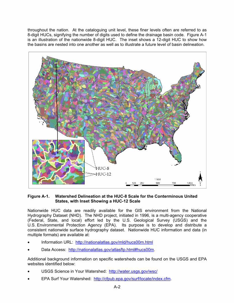
A-2
throughout the nation. At the cataloguing unit level, these finer levels often are referred to as 8-digit HUCs, signifying the number of digits used to define the drainage basin code. Figure A-1 is an illustration of the nationwide 8-digit HUC. The inset shows a 12-digit HUC to show how the basins are nested into one another as well as to illustrate a future level of basin delineation.
Figure A-1. Watershed Delineation at the HUC-8 Scale for the Conterminous United States, with Inset Showing a HUC-12 Scale
Nationwide HUC data are readily available for the GIS environment from the National Hydrography Dataset (NHD). The NHD project, initiated in 1996, is a multi-agency cooperative (Federal, State, and local) effort led by the U.S. Geological Survey (USGS) and the U.S. Environmental Protection Agency (EPA). Its purpose is to develop and distribute a consistent nationwide surface hydrography dataset. Nationwide HUC information and data (in multiple formats) are available at:
• Information URL: http://nationalatlas.gov/mld/hucs00m.html
• Data Access: http://nationalatlas.gov/atlasftp.html#hucs00m.
Additional background information on specific watersheds can be found on the USGS and EPA websites identified below:
• USGS Science in Your Watershed: http://water.usgs.gov/wsc/
• EPA Surf Your Watershed: http://cfpub.epa.gov/surf/locate/index.cfm.

A-3
A.2.2 Stream Networks/Waterbodies
Routed and attributed stream networks and waterbodies are available under the NHD program at three primary scales: (1) Medium Resolution (1:100,000 scale), (2) High Resolution (1:24,000 scale), and (3) Local Resolution (<1:24,000, scale varies). While the local resolution data are not available throughout the conterminous United States, the High Resolution and Medium Resolution datasets are available. The NHD website (URL provided below) offers an interactive viewer to assess the availability of data for a given area. The website viewer also allows for interactive downloading of data. Alternatively, the NHD allows users to retrieve data for an entire 4-digit HUC; these data, called “pre-staged” data, are maintained as current as data available in the interactive viewer. Data can be accessed via file transfer protocol (FTP) links (uniform resource locators [URLs] provided below) and are available in several formats including Environmental Systems Research Institute (ESRI) coverage format, shapefile format, and personal geodatabase. The shapefile format is a de facto standard in geospatial data; thus, it should be usable by most GIS software products, in addition to ESRI products such as ArcGIS and Arc/INFO. The geodatabase format represents a new advanced geospatial file format containing multiple spatial data elements that can be linked and interact with one another through developed rule sets. The disadvantage to using the geodatabase file format is that it is limited to certain commercial software products such as ArcGIS and ERDAS Imagine. More information about the personal geodatabase can be found on the ESRI website at http://www.esri.com/software/arcgis/geodatabase/index.html.
• Information URL: http://nhd.usgs.gov/
• Data Access:
– Pre-Staged Data: ftp://nhdftp.usgs.gov/SubRegions/
– Interactive Viewer: http://nhd.usgs.gov/data.html
A.2.3 Digital Elevation Models
Digital Elevation Models (DEMs) provide the basis for most hydrologic modeling and represent the earth’s surface at the ground level, often referred to as “bare earth.” This approach provides a representation of the terrain surface without obstruction from trees or buildings, and in the case of large waterbodies, an average water-surface elevation is used. A DEM is composed of a regular grid of points that represents a sample elevation with the specified resolution of the dataset. DEMs for the United States are available for most places at 10-m resolution, and full coverage is available at 30- and 90-m resolutions.
DEMs are available from many sources and are available at several different resolutions.
• Information URL:
– National Elevation Dataset (NED): http://ned.usgs.gov/
– Shuttle Radar Topographic Mission (SRTM): http://www2.jpl.nasa.gov/srtm/
– The National Digital Elevation Program: http://www.ndep.gov/.
• Data Access:
– USGS Seamless Server: http://seamless.usgs.gov.
The USGS Seamless Server provides access to several different sources and resolutions of DEM data, including the NED in 1-arc-second (~30-m), 1/3-arc-second (~10-m), and in limited areas 1/9-arc-second resolutions (~3-m). The SRTM data are available at 3-arc-second and
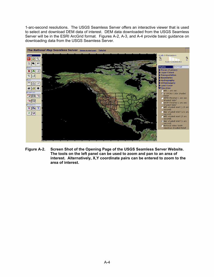
A-4
1-arc-second resolutions. The USGS Seamless Server offers an interactive viewer that is used to select and download DEM data of interest. DEM data downloaded from the USGS Seamless Server will be in the ESRI ArcGrid format. Figures A-2, A-3, and A-4 provide basic guidance on downloading data from the USGS Seamless Server.
Figure A-2. Screen Shot of the Opening Page of the USGS Seamless Server Website. The tools on the left panel can be used to zoom and pan to an area of interest. Alternatively, X,Y coordinate pairs can be entered to zoom to the area of interest.

A-5
Figure A-3. Seamless Server Layers Can Be Turned On and Off on the Right Panel, Which Helps to Navigate and Identify the Area of Interest. When the area of interest has been identified, change the tab on the right panel to “Download,” and select the layers of interest (note: it is possible to download more than just DEM data here), then use the Download tools on the left-panel to select an area for downloading.
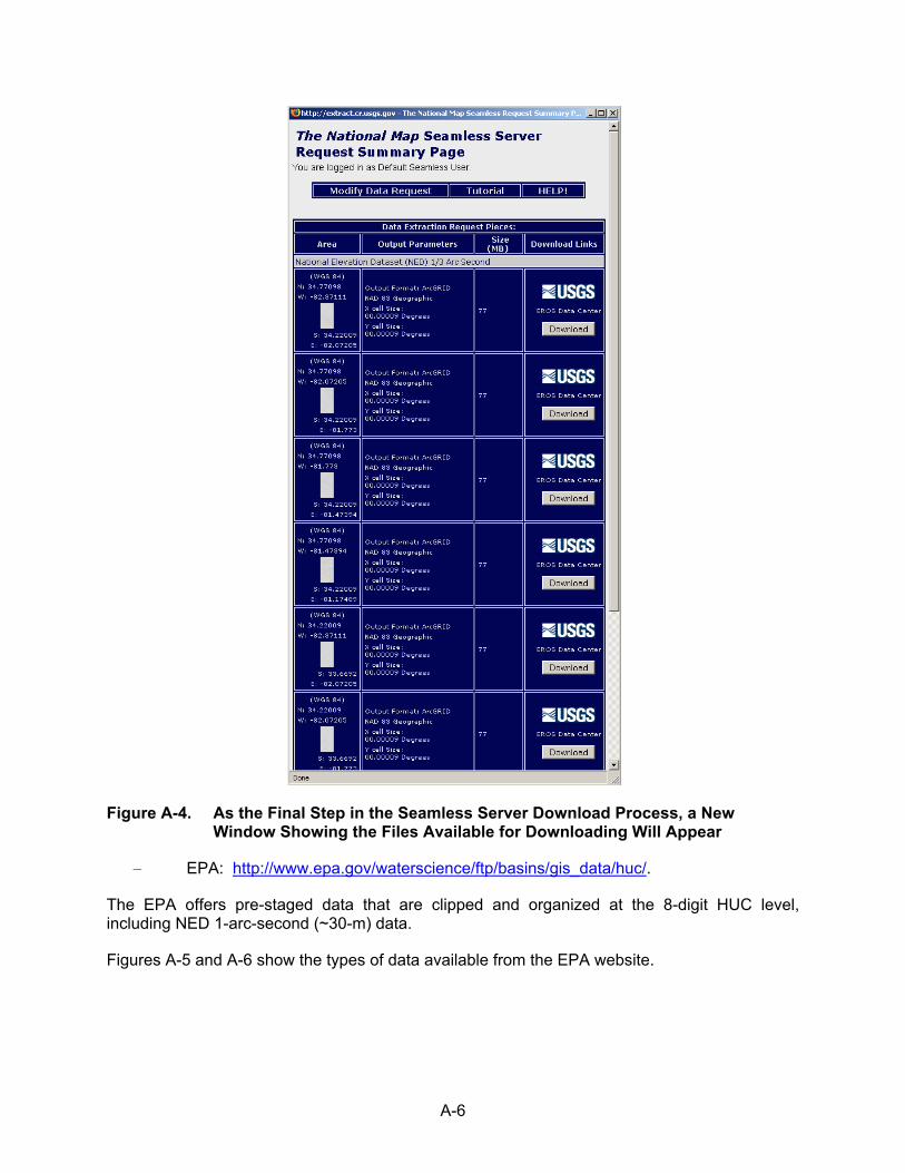
A-6
Figure A-4. As the Final Step in the Seamless Server Download Process, a New Window Showing the Files Available for Downloading Will Appear
– EPA: http://www.epa.gov/waterscience/ftp/basins/gis_data/huc/.
The EPA offers pre-staged data that are clipped and organized at the 8-digit HUC level, including NED 1-arc-second (~30-m) data.
Figures A-5 and A-6 show the types of data available from the EPA website.

A-7
Figure A-5. EPA Data Access Organized by 8-digit HUCs. The folders are named after the 8-digit HUCs.
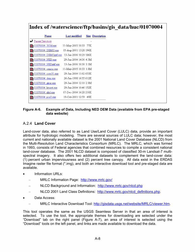
A-8
Figure A-6. Example of Data, Including NED DEM Data (available from EPA pre-staged data website)
A.2.4 Land Cover
Land-cover data, also referred to as Land Use/Land Cover (LULC) data, provide an important attribute for hydrologic modeling. There are several sources of LULC data; however, the most current and nationally available dataset is the 2001 National Land Cover Database (NLCD) from the Multi-Resolution Land Characteristics Consortium (MRLC). The MRLC, which was formed in 1993, consists of Federal agencies that combined resources to compile a consistent national land-cover database. The 2001 NLCD dataset is composed of classified 30-m Landsat-7 multi-spectral imagery. It also offers two additional datasets to complement the land-cover data: (1) percent urban imperviousness and (2) percent tree canopy. All data exist in the ERDAS Imagine raster file format (*.img), and both an interactive download tool and pre-staged data are available.
• Information URLs:
– MRLC Information Page: http://www.mrlc.gov/
– NLCD Background and Information: http://www.mrlc.gov/nlcd.php
– NLCD 2001 Land Class Definitions: http://www.mrlc.gov/nlcd_definitions.php.
• Data Access:
– MRLC Interactive Download Tool: http://gisdata.usgs.net/website/MRLC/viewer.htm.
This tool operates the same as the USGS Seamless Server in that an area of interest is selected. To use the tool, the appropriate themes for downloading are selected under the “Download” tab on the right panel (Figure A-7), an area of interest is selected using the “Download” tools on the left panel, and links are made available to download the data.
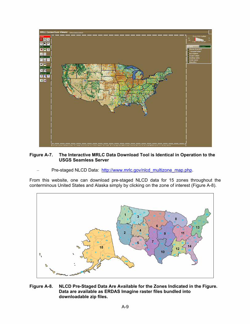
A-9
Figure A-7. The Interactive MRLC Data Download Tool is Identical in Operation to the USGS Seamless Server
– Pre-staged NLCD Data: http://www.mrlc.gov/nlcd_multizone_map.php.
From this website, one can download pre-staged NLCD data for 15 zones throughout the conterminous United States and Alaska simply by clicking on the zone of interest (Figure A-8).
Figure A-8. NLCD Pre-Staged Data Are Available for the Zones Indicated in the Figure. Data are available as ERDAS Imagine raster files bundled into downloadable zip files.
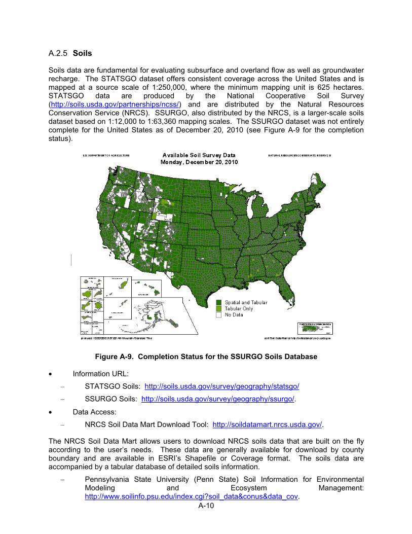
A-10
A.2.5 Soils
Soils data are fundamental for evaluating subsurface and overland flow as well as groundwater recharge. The STATSGO dataset offers consistent coverage across the United States and is mapped at a source scale of 1:250,000, where the minimum mapping unit is 625 hectares. STATSGO data are produced by the National Cooperative Soil Survey (http://soils.usda.gov/partnerships/ncss/) and are distributed by the Natural Resources Conservation Service (NRCS). SSURGO, also distributed by the NRCS, is a larger-scale soils dataset based on 1:12,000 to 1:63,360 mapping scales. The SSURGO dataset was not entirely complete for the United States as of December 20, 2010 (see Figure A-9 for the completion status).
Figure A-9. Completion Status for the SSURGO Soils Database
• Information URL:
– STATSGO Soils: http://soils.usda.gov/survey/geography/statsgo/
– SSURGO Soils: http://soils.usda.gov/survey/geography/ssurgo/.
• Data Access:
– NRCS Soil Data Mart Download Tool: http://soildatamart.nrcs.usda.gov/.
The NRCS Soil Data Mart allows users to download NRCS soils data that are built on the fly according to the user’s needs. These data are generally available for download by county boundary and are available in ESRI’s Shapefile or Coverage format. The soils data are accompanied by a tabular database of detailed soils information.
– Pennsylvania State University (Penn State) Soil Information for Environmental Modeling and Ecosystem Management: http://www.soilinfo.psu.edu/index.cgi?soil_data&conus&data_cov.
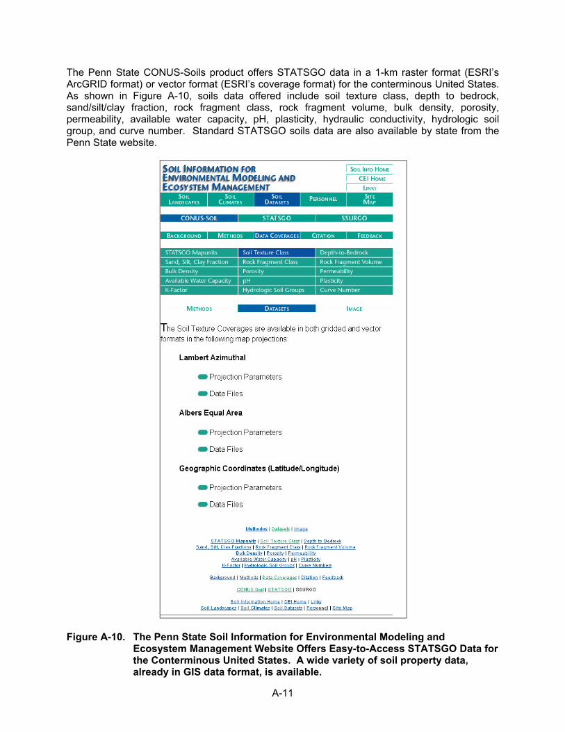
A-11
The Penn State CONUS-Soils product offers STATSGO data in a 1-km raster format (ESRI’s ArcGRID format) or vector format (ESRI’s coverage format) for the conterminous United States. As shown in Figure A-10, soils data offered include soil texture class, depth to bedrock, sand/silt/clay fraction, rock fragment class, rock fragment volume, bulk density, porosity, permeability, available water capacity, pH, plasticity, hydraulic conductivity, hydrologic soil group, and curve number. Standard STATSGO soils data are also available by state from the Penn State website.
Figure A-10. The Penn State Soil Information for Environmental Modeling and Ecosystem Management Website Offers Easy-to-Access STATSGO Data for the Conterminous United States. A wide variety of soil property data, already in GIS data format, is available.

A-12
– EPA: http://www.epa.gov/waterscience/ftp/basins/statsgo/.
Similar to the DEM offerings from the EPA, STATSGO data also are available in a pre-staged format that is clipped and organized at the state level (Figure A-11).
Figure A-11. Pre-Staged STATSGO Data Available at the EPA Website
A.2.6 Dam Locations
The location and statistics of dams within a watershed may be of interest. The U.S. Army Corps of Engineers maintains the National Inventory of Dams, which is available from the National Atlas website referenced below.
• National Inventory of Dams: http://crunch.tec.army.mil/nidpublic/webpages/nid.cfm
• Data Access: http://nationalatlas.gov/mld/dams00x.html.
A-13
A.2.7 Other Miscellaneous Geospatial Data of Interest
• USGS Geospatial Hydrologic Data: http://water.usgs.gov/lookup/getgislist
• The National Map: http://nmviewogc.cr.usgs.gov/viewer.htm
• The National Atlas: http://nationalatlas.gov/atlasftp.html.
A.3 References
Kelmelis, J.A. 1998. “Process Dynamics, Temporal Extent, and Causal Propagation as the Basis for Linking Space and Time.” In: Spatial and Temporal Reasoning in Geographic Information Systems, Oxford University Press, Oxford, England.
U.S. Geological Survey (USGS). 2008. Hydrologic Unit Maps. Available at http://water.usgs.gov/GIS/huc.html. Accessed May 30, 2008.

Appendix B
FLOODING FROM LOCAL INTENSE PRECIPITATION: A CASE STUDY

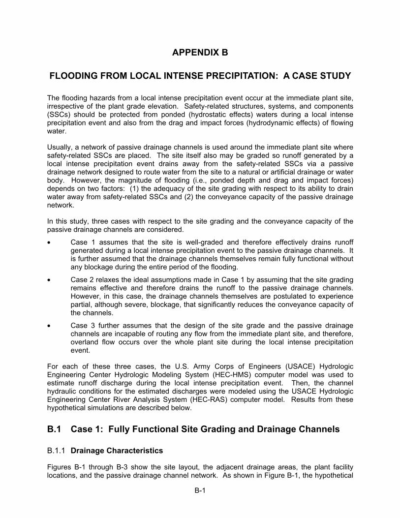
B-1
APPENDIX B
FLOODING FROM LOCAL INTENSE PRECIPITATION: A CASE STUDY
The flooding hazards from a local intense precipitation event occur at the immediate plant site, irrespective of the plant grade elevation. Safety-related structures, systems, and components (SSCs) should be protected from ponded (hydrostatic effects) waters during a local intense precipitation event and also from the drag and impact forces (hydrodynamic effects) of flowing water.
Usually, a network of passive drainage channels is used around the immediate plant site where safety-related SSCs are placed. The site itself also may be graded so runoff generated by a local intense precipitation event drains away from the safety-related SSCs via a passive drainage network designed to route water from the site to a natural or artificial drainage or water body. However, the magnitude of flooding (i.e., ponded depth and drag and impact forces) depends on two factors: (1) the adequacy of the site grading with respect to its ability to drain water away from safety-related SSCs and (2) the conveyance capacity of the passive drainage network.
In this study, three cases with respect to the site grading and the conveyance capacity of the passive drainage channels are considered.
• Case 1 assumes that the site is well-graded and therefore effectively drains runoff generated during a local intense precipitation event to the passive drainage channels. It is further assumed that the drainage channels themselves remain fully functional without any blockage during the entire period of the flooding.
• Case 2 relaxes the ideal assumptions made in Case 1 by assuming that the site grading remains effective and therefore drains the runoff to the passive drainage channels. However, in this case, the drainage channels themselves are postulated to experience partial, although severe, blockage, that significantly reduces the conveyance capacity of the channels.
• Case 3 further assumes that the design of the site grade and the passive drainage channels are incapable of routing any flow from the immediate plant site, and therefore, overland flow occurs over the whole plant site during the local intense precipitation event.
For each of these three cases, the U.S. Army Corps of Engineers (USACE) Hydrologic Engineering Center Hydrologic Modeling System (HEC-HMS) computer model was used to estimate runoff discharge during the local intense precipitation event. Then, the channel hydraulic conditions for the estimated discharges were modeled using the USACE Hydrologic Engineering Center River Analysis System (HEC-RAS) computer model. Results from these hypothetical simulations are described below.
B.1 Case 1: Fully Functional Site Grading and Drainage Channels
B.1.1 Drainage Characteristics
Figures B-1 through B-3 show the site layout, the adjacent drainage areas, the plant facility locations, and the passive drainage channel network. As shown in Figure B-1, the hypothetical
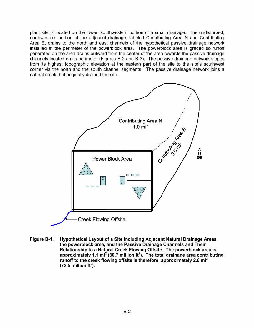
B-2
plant site is located on the lower, southwestern portion of a small drainage. The undisturbed, northwestern portion of the adjacent drainage, labeled Contributing Area N and Contributing Area E, drains to the north and east channels of the hypothetical passive drainage network installed at the perimeter of the powerblock area. The powerblock area is graded so runoff generated on the area drains outward from the center of the area towards the passive drainage channels located on its perimeter (Figures B-2 and B-3). The passive drainage network slopes from its highest topographic elevation at the eastern part of the site to the site’s southwest corner via the north and the south channel segments. The passive drainage network joins a natural creek that originally drained the site.
Figure B-1. Hypothetical Layout of a Site Including Adjacent Natural Drainage Areas, the powerblock area, and the Passive Drainage Channels and Their Relationship to a Natural Creek Flowing Offsite. The powerblock area is approximately 1.1 mi2 (30.7 million ft2). The total drainage area contributing runoff to the creek flowing offsite is therefore, approximately 2.6 mi2 (72.5 million ft2).
NN
Contributing Area N1.0 mi2
Con
tribu
ting
Area
E
0.5
mi2
Power Block Area
Creek Flowing Offsite
NNNN
Contributing Area N1.0 mi2
Con
tribu
ting
Area
E
0.5
mi2
Power Block Area
Creek Flowing Offsite
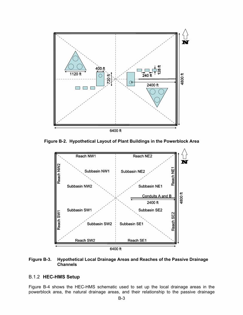
B-3
Figure B-2. Hypothetical Layout of Plant Buildings in the Powerblock Area
Figure B-3. Hypothetical Local Drainage Areas and Reaches of the Passive Drainage Channels
B.1.2 HEC-HMS Setup
Figure B-4 shows the HEC-HMS schematic used to set up the local drainage areas in the powerblock area, the natural drainage areas, and their relationship to the passive drainage
400 ft
720
ft1120 ft
6400 ft
4800
ft
2400 ft
240 ft 128
ft
NN
400 ft
720
ft1120 ft
6400 ft
4800
ft
2400 ft
240 ft240 ft 128
ft12
8 ft
NN
6400 ft
4800
ft
2400 ft
Conduits A and B
NN
Subbasin NE1
Subbasin NE2Subbasin NW1
Subbasin NW2
Subbasin SW1
Subbasin SW2 Subbasin SE1
Subbasin SE2
Re
ach
NE
1
Reach NE2Reach NW1
Reach SW2
Re
ach
NW
2R
eac
h S
W1
Rea
ch S
E2
Reach SE1
6400 ft
4800
ft
2400 ft
Conduits A and B
NN
Subbasin NE1
Subbasin NE2Subbasin NW1
Subbasin NW2
Subbasin SW1
Subbasin SW2 Subbasin SE1
Subbasin SE2
Re
ach
NE
1
Reach NE2Reach NW1
Reach SW2
Re
ach
NW
2R
eac
h S
W1
Rea
ch S
E2
Reach SE1
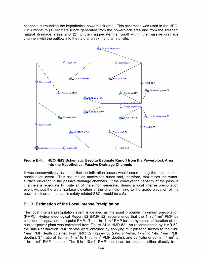
B-4
channels surrounding the hypothetical powerblock area. This schematic was used in the HEC-HMS model to (1) estimate runoff generated from the powerblock area and from the adjacent natural drainage areas and (2) to then aggregate the runoff within the passive drainage channels with the outflow into the natural creek that drains offsite.
Figure B-4. HEC-HMS Schematic Used to Estimate Runoff from the Powerblock Area into the Hypothetical Passive Drainage Channels
It was conservatively assumed that no infiltration losses would occur during the local intense precipitation event. This assumption maximizes runoff and, therefore, maximizes the water-surface elevation in the passive drainage channels. If the conveyance capacity of the passive channels is adequate to route all of the runoff generated during a local intense precipitation event without the water-surface elevation in the channels rising to the grade elevation of the powerblock area, the plant’s safety-related SSCs would be safe.
B.1.3 Estimation of the Local Intense Precipitation
The local intense precipitation event is defined as the point probable maximum precipitation (PMP). Hydrometeorlogical Report 52 (HMR 52) recommends that the 1-hr, 1-mi2 PMP be considered equivalent to a point PMP. The 1-hr, 1-mi2 PMP for the hypothetical location of the nuclear power plant was estimated from Figure 24 in HMR 52. As recommended by HMR 52, the sub-1-hr duration PMP depths were obtained by applying multiplication factors to the 1-hr, 1-mi2 PMP depth obtained from HMR 52 Figures 36 (ratio of 5-min, 1-mi2 to 1-hr, 1-mi2 PMP depths), 37 (ratio of 15-min, 1-mi2 to 1-hr, 1-mi2 PMP depths), and 38 (ratio of 30-min, 1-mi2 to 1-hr, 1-mi2 PMP depths). The 6-hr, 10-mi2 PMP depth can be obtained either directly from
B-5
HMR 51, or by using the ratio of 1-hr, 1-mi2 to 6-hr, 10-mi2 PMP depths given in Figure 23 of HMR 52). Table B-1 below lists the estimated local intense precipitation for the hypothetical location of the nuclear power plant.
Table B-1. Local Intense Precipitation for the Hypothetical Nuclear Power Plant
Duration Area (mi2) Multiplier Applied to
Local Intense Precipitation (in.)
6 hr 10 1.0/0.621 (HMR 52 Figure 23)
1-hr, 1-mi2 PMP 31.0
1 hr 1 NA NA 19.3 (HMR 52 Figure 24)
30 min 1 0.738 (HMR 52 Figure 38)
1-hr, 1-mi2 PMP 14.2
15 min 1 0.509 (HMR 52 Figure 37)
1-hr, 1-mi2 PMP 9.8
5 min 1 0.323 (HMR 52 Figure 36)
1-hr, 1-mi2 PMP 6.2
B.1.4 Estimation of Runoff Hydrographs
The local intense precipitation shown in Table B-1 was input into the HEC-HMS modeling system with a 5-minute time step. The first time step was set to the highest local intense precipitation depth, which is 6.2 in. The next two 5-minute time steps were set to an incremental precipitation depth of 1.8 in. ([9.8 - 6.2]/2 in.). Incremental precipitation depths for the subsequent time steps were determined from the cumulative local intense precipitation depths shown in Table B-1. The hyetograph of the local intense precipitation event on the hypothetical nuclear power plant site is shown in Figure B-5.
It was conservatively assumed that the 1-hr, 1-mi2 PMP would occur uniformly over the 2.6-mi2 local drainage. It was also conservatively assumed that the antecedent moisture conditions in the local drainage would be such that no rainfall losses would occur over the duration of the PMP event and the subsequent runoff events (i.e., the loss rate in the HEC-HMS basin model for each of the powerblock area subbasins and Contributing Areas N and E were set to “None”).
HEC-HMS also requires that a Transform Method be specified for each subbasin. The Transform Method determines the temporal distribution of the runoff generated from the sub-basin. A unit hydrograph (UH) approach was adopted. The UH used for the subbasins in the powerblock area and Contributing Areas N and E were based on the Soil Conservation Service (i.e., SCS; now the Natural Resources Conservation Service [NRCS]) synthetic graph applicable to drainage areas 2000 ac or smaller (SCS 1972). The UH approach to estimating runoff from rainfall excess is based on an assumption of linearity. This assumption postulates that the direct runoff hydrograph from a unit depth of rainfall excess is the UH and the direct runoff hydrograph for any other amount of rainfall excess can be estimated by scaling the ordinates of the UH by the corresponding rainfall excess (e.g., the ordinates of the direct runoff hydrograph corresponding to two units of rainfall excess are simply the ordinates of the UH multiplied by two). Traditionally, UH is derived from observed rainfall-runoff events. Where adequate observations of rainfall-runoff are not available, regionalized, synthetic UHs based on rainfall-
B-6
runoff from similar drainage catchments have been developed (e.g., the SCS UH [SCS 1972] and the Snyder UH [Snyder 1938]). The recommendation for the applicability of these methods includes the size of the drainage catchment. The SCS UH is recommended for areas of 2000 ac (3.1 mi2) or less, and the Snyder UH is recommended for areas of 10 to 10,000 mi2.
Figure B-5. Hyetograph of the Local Intense Precipitation Event on the Hypothetical Nuclear Power Plant Site
The UH linearity assumption starts to break down as the rainfall intensity and volume increase to the magnitudes of the PMP event. During the PMP event, the large amount of rainfall excess causes the runoff mechanism to be dominated by highly non-linear hydraulic effects in the overland flow process. Surface roughness resulting from small irregularities may be subsumed by the greater depth of the overland flow, thereby increasing the likelihood of quicker delivery of overland flow to the channel network. When possible, unit hydrographs based on severe storms approaching the magnitude of a PMP event in the drainage basin of concern should be used. Therefore, USACE suggests that an adjustment to the traditional UH derived from observations of storms of smaller magnitudes is required to account for the more rapid overland flow response during storm events that approach the PMP (USACE 1994; see page 7-1).
USACE also recommends that for large storms, the time to peak for the UH estimated from smaller storms be reduced (USACE 1994; see page 13-8). Other authors (Pilgrim and Cordery 1993) have suggested that the peak discharge be increased by 20 to 50 percent and time-to-peak be reduced by 33 percent. In the absence of specific guidance, the following UH adjustment method was adopted as reasonably conservative for this study:
1. Reduce time-to-peak by 33 percent.
2. Increase peak discharge by 20 percent.
3. Ensure that the area under the UH, representing the volume of excess runoff, is equivalent to unit rainfall excess over the drainage basin.
The 6-hr Local Intense Precipitation Hyetograph
Time (min)
Pre
cip
itatio
n D
ep
th (
in)
0 30 60 90 120 150 180 210 240 270 300 330 360
0.0
0.5
1.0
1.5
2.0
2.5
3.0
3.5
4.0
4.5
5.0
5.5
6.0
6.56.200
1.8001.467
0.850
0.195
B-7
Where possible, a different adjustment method, supported by data in the drainage basin of concern, may be used. In these instances, a complete description of the method, the supporting data, and a justification should be presented.
The modified SCS UH for the sub-basins in the powerblock area and Contributing Areas N and E were input into the HEC-HMS modeling system, which was set to use “User-Specified Unit Hydrograph” as the Transform Method for all sub-areas of the local drainage. Runoff from the drainage sub-areas would collect in the hypothetical passive drainage channels and be carried offsite. Kinematic wave routing was used for the drainage channels labeled NE1, NE2, NW1, NW2, SW1, SW2, SE1, and SE2 (see Figure B-4 above). The Manning’s roughness coefficient for all these drainage channels was set to 0.024 (Chow 1959). All channels were assumed to have a bottom width of 15 ft and side slope of 3:1 (H:V). Lag routing with a lag time of 5 minutes was used for channels RDE and RDW.
The HEC-HMS model was used to simulate the direct runoff hydrograph for the drainage channels. Figure B-6 shows the HEC-HMS simulated runoff discharge hydrograph at the outlet (the southwestern corner of the hypothetical passive drainage channel network). The peak discharges in all reaches were determined from the HEC-HMS simulations.
Figure B-6. Direct Runoff Hydrograph at the Outlet of the Hypothetical Passive Drainage Network
B.1.5 Estimation of Water-Surface Elevations
The site grade elevation in the powerblock area is assumed to be 200 ft. The bottom elevations of channel reaches at specific points are shown in Table B-2. A conservative approach for estimating the bounding water-surface elevation in the hypothetical passive drainage channel network is to assume (1) that the peak discharges in all channel reaches occur simultaneously and (2) that these peak discharges represent steady-state conditions. These assumptions are conservative and would lead to estimates of a higher water-surface elevation in individual reaches than what would be expected during transient conditions that would actually occur
Discharge Hydrograph at the Outlet
Time
Dis
cha
rge
(cf
s)
0:00
1:00
2:00
3:00
4:00
5:00
6:00
7:00
8:00
9:00
10:0
0
11:0
0
12:0
0
13:0
0
14:0
0
15:0
0
16:0
0
17:0
0
18:0
0
0
2000
4000
6000
8000
10000
B-8
during the local intense precipitation event. Therefore, the estimated water-surface elevations would be a bounding estimate.
Table B-2 shows the HEC-HMS estimated peak discharges for all reaches of the hypothetical passive drainage network. The peak discharge at the outlet occurred 2 hr and 1 minute after the start of the local intense precipitation event. The peak discharges and the corresponding times for each of the reaches are shown in column 2. Column 3 shows the estimated discharge in each reach at the time corresponding to the peak discharge at the outlet.
Table B-2. Comparison of Peak Discharges and Corresponding Times for Each Reach and the Discharges in Each Reach Corresponding to the Time of Peak Discharge at the Outlet
Reach Upstream Bottom
Elevation (ft) Peak Discharge and Time§ (cfs)
[Time (hr:min)] Discharge at 2:01
(cfs)
NE1 180.0 1520.5 [1:58] 1518.0
NE2 175.2 5699.6 [2:15] 5632.7
NW1 168.8 6339.4 [2:05] 6318.4
NW2 162.4 6900.2 [2:05] 6878.2
SW1 157.6 7544.6 [2:04] 7526.2
SW2 164.0 3146.2 [1:29] 2888.5
SE1 175.2 2241.0 [1:32] 2153.8
SE2 180.0 1430.5 [1:59] 1429.9
RDE - 1619.2 [0:10] 50.9
RDW - 1619.2 [0:10] 50.9
Outlet 152.4 10414.7 [2:01] 10414.7 § The discharges used in the steady-state, water-surface-profile simulations are indicated in boldface.
Apart from reaches SW2, SE1, RDE, and RDW, the times of peak discharge in all reaches are within a few minutes of the time of peak discharge at the outlet point (i.e., 2 hr and 1 min). Therefore, in the HEC-RAS steady-state, water-surface profile simulations, the discharge in each reach except for the four reaches mentioned above were set to their own peak discharge rates. Because the times of the peak discharges in the four reaches are significantly earlier than those at the outlet, these peak discharges would pass through the outlet before the outlet discharge reaches its peak and, therefore, would not significantly affect the peak outlet discharge. The discharges for the four reaches whose peak-discharge times were significantly different from the outlet peak discharge time were set to their respective estimated discharge at 2 hr and 1 min, which corresponds to the time of outlet peak discharge.
The HEC-RAS model was set up for the hypothetical passive drainage channel network as shown in Figure B-7. A steady-state simulation was performed using the estimated discharges obtained from the HEC-HMS simulation as explained above. Uniform, trapezoidal cross sections for all channels with bottom widths of 40 ft and side slopes of 3:1 (H:V) were assumed. Intermediate cross sections required by the HEC-RAS computations were interpolated within the software package. Figures B-8 through B-11 show simulated cross sections with water-surface elevations at key points in the hypothetical passive drainage channel network.
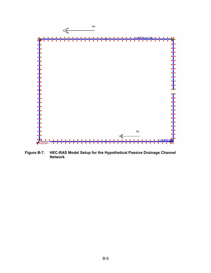
B-9
Figure B-7. HEC-RAS Model Setup for the Hypothetical Passive Drainage Channel Network
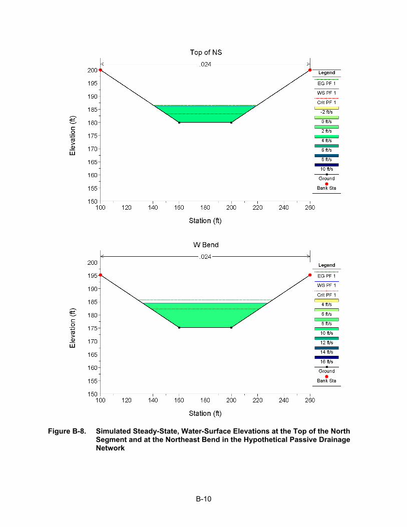
B-10
Figure B-8. Simulated Steady-State, Water-Surface Elevations at the Top of the North Segment and at the Northeast Bend in the Hypothetical Passive Drainage Network
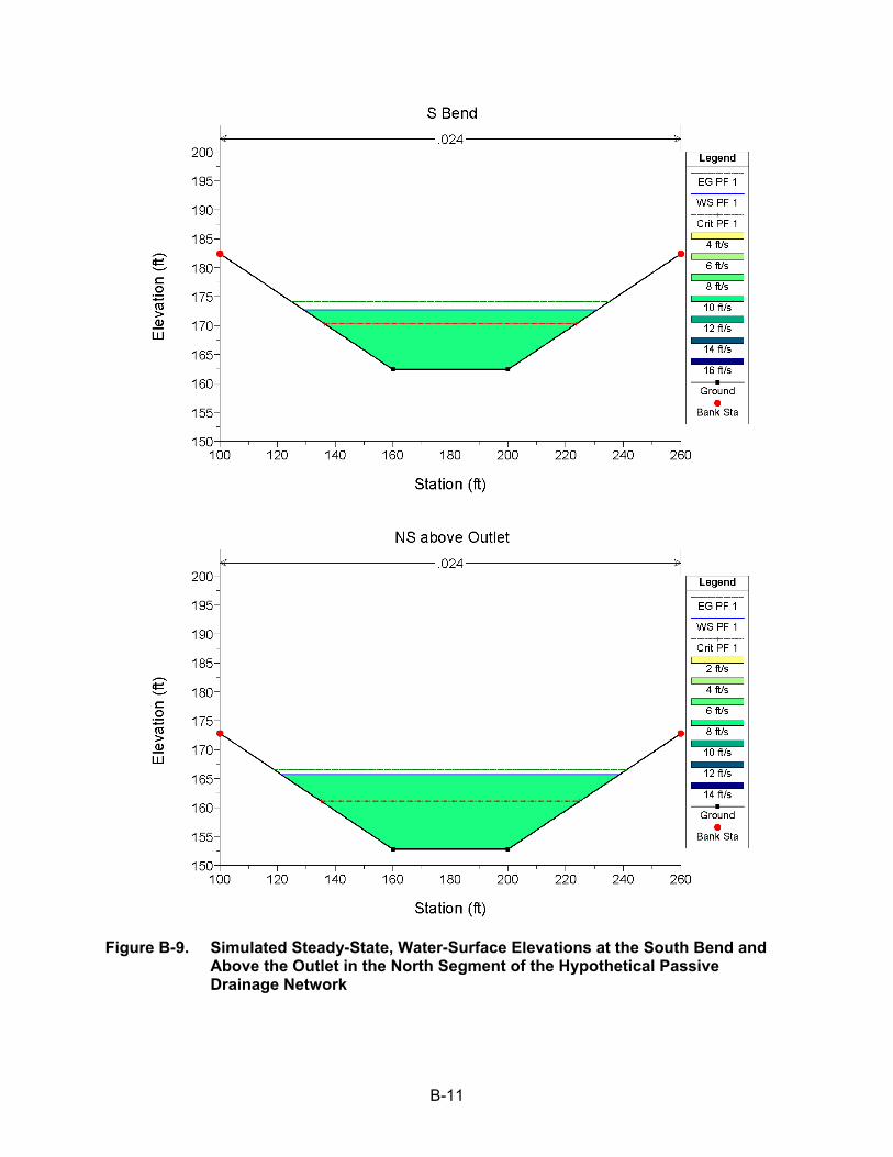
B-11
Figure B-9. Simulated Steady-State, Water-Surface Elevations at the South Bend and Above the Outlet in the North Segment of the Hypothetical Passive Drainage Network
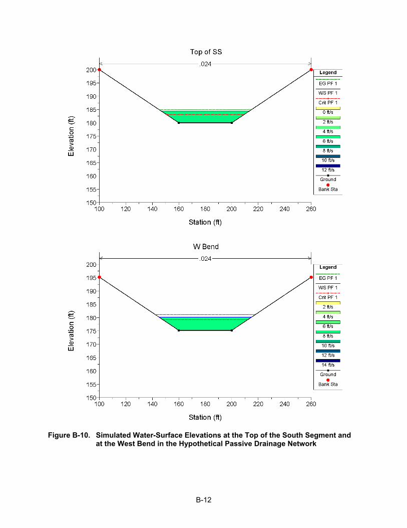
B-12
Figure B-10. Simulated Water-Surface Elevations at the Top of the South Segment and at the West Bend in the Hypothetical Passive Drainage Network
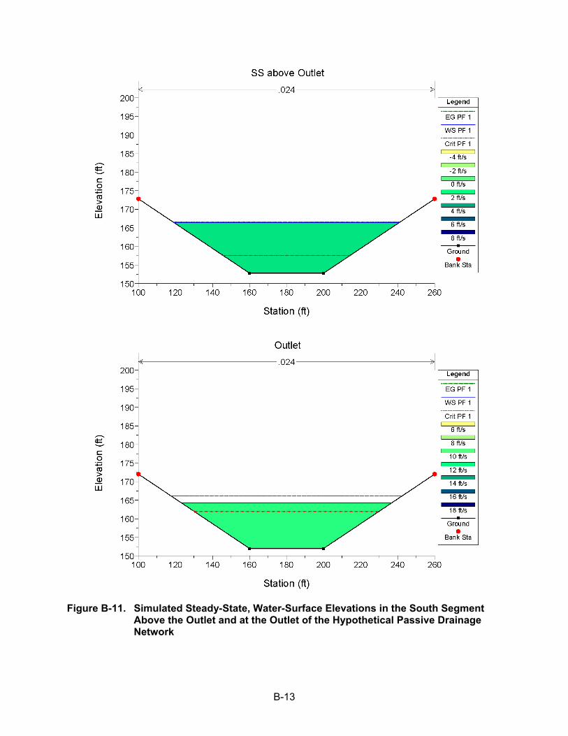
B-13
Figure B-11. Simulated Steady-State, Water-Surface Elevations in the South Segment Above the Outlet and at the Outlet of the Hypothetical Passive Drainage Network
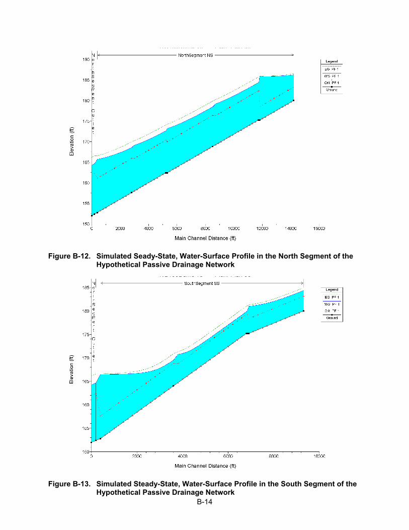
B-14
Figure B-12. Simulated Seady-State, Water-Surface Profile in the North Segment of the Hypothetical Passive Drainage Network
Figure B-13. Simulated Steady-State, Water-Surface Profile in the South Segment of the Hypothetical Passive Drainage Network
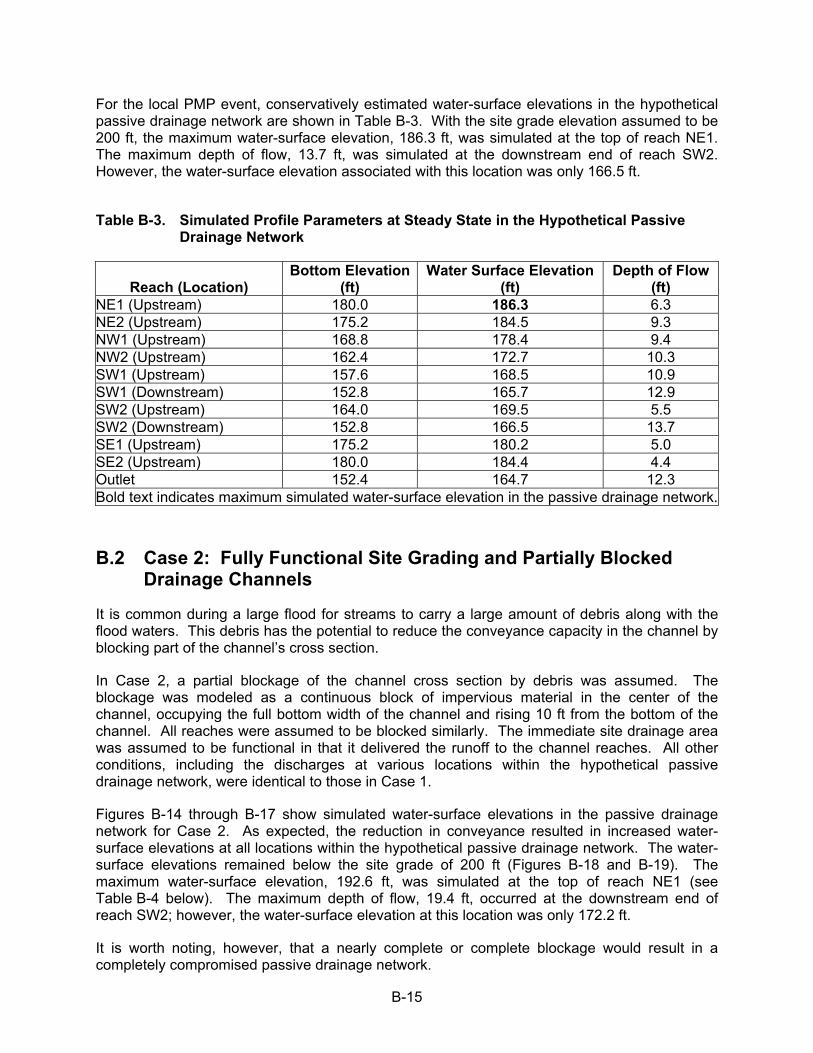
B-15
For the local PMP event, conservatively estimated water-surface elevations in the hypothetical passive drainage network are shown in Table B-3. With the site grade elevation assumed to be 200 ft, the maximum water-surface elevation, 186.3 ft, was simulated at the top of reach NE1. The maximum depth of flow, 13.7 ft, was simulated at the downstream end of reach SW2. However, the water-surface elevation associated with this location was only 166.5 ft.
Table B-3. Simulated Profile Parameters at Steady State in the Hypothetical Passive Drainage Network
Reach (Location) Bottom Elevation
(ft) Water Surface Elevation
(ft) Depth of Flow
(ft) NE1 (Upstream) 180.0 186.3 6.3 NE2 (Upstream) 175.2 184.5 9.3 NW1 (Upstream) 168.8 178.4 9.4 NW2 (Upstream) 162.4 172.7 10.3 SW1 (Upstream) 157.6 168.5 10.9 SW1 (Downstream) 152.8 165.7 12.9 SW2 (Upstream) 164.0 169.5 5.5 SW2 (Downstream) 152.8 166.5 13.7 SE1 (Upstream) 175.2 180.2 5.0 SE2 (Upstream) 180.0 184.4 4.4 Outlet 152.4 164.7 12.3 Bold text indicates maximum simulated water-surface elevation in the passive drainage network.
B.2 Case 2: Fully Functional Site Grading and Partially Blocked Drainage Channels
It is common during a large flood for streams to carry a large amount of debris along with the flood waters. This debris has the potential to reduce the conveyance capacity in the channel by blocking part of the channel’s cross section.
In Case 2, a partial blockage of the channel cross section by debris was assumed. The blockage was modeled as a continuous block of impervious material in the center of the channel, occupying the full bottom width of the channel and rising 10 ft from the bottom of the channel. All reaches were assumed to be blocked similarly. The immediate site drainage area was assumed to be functional in that it delivered the runoff to the channel reaches. All other conditions, including the discharges at various locations within the hypothetical passive drainage network, were identical to those in Case 1.
Figures B-14 through B-17 show simulated water-surface elevations in the passive drainage network for Case 2. As expected, the reduction in conveyance resulted in increased water-surface elevations at all locations within the hypothetical passive drainage network. The water-surface elevations remained below the site grade of 200 ft (Figures B-18 and B-19). The maximum water-surface elevation, 192.6 ft, was simulated at the top of reach NE1 (see Table B-4 below). The maximum depth of flow, 19.4 ft, occurred at the downstream end of reach SW2; however, the water-surface elevation at this location was only 172.2 ft.
It is worth noting, however, that a nearly complete or complete blockage would result in a completely compromised passive drainage network.
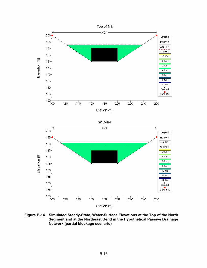
B-16
Figure B-14. Simulated Steady-State, Water-Surface Elevations at the Top of the North Segment and at the Northeast Bend in the Hypothetical Passive Drainage Network (partial blockage scenario)
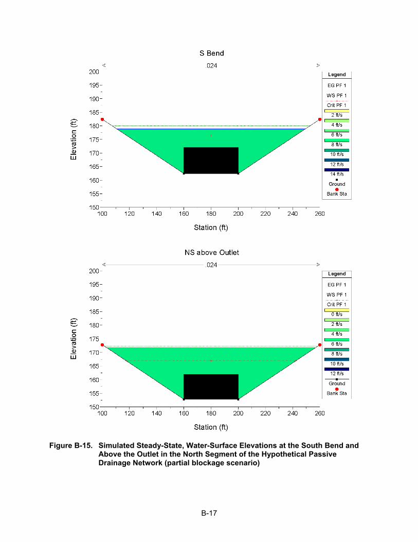
B-17
Figure B-15. Simulated Steady-State, Water-Surface Elevations at the South Bend and Above the Outlet in the North Segment of the Hypothetical Passive Drainage Network (partial blockage scenario)
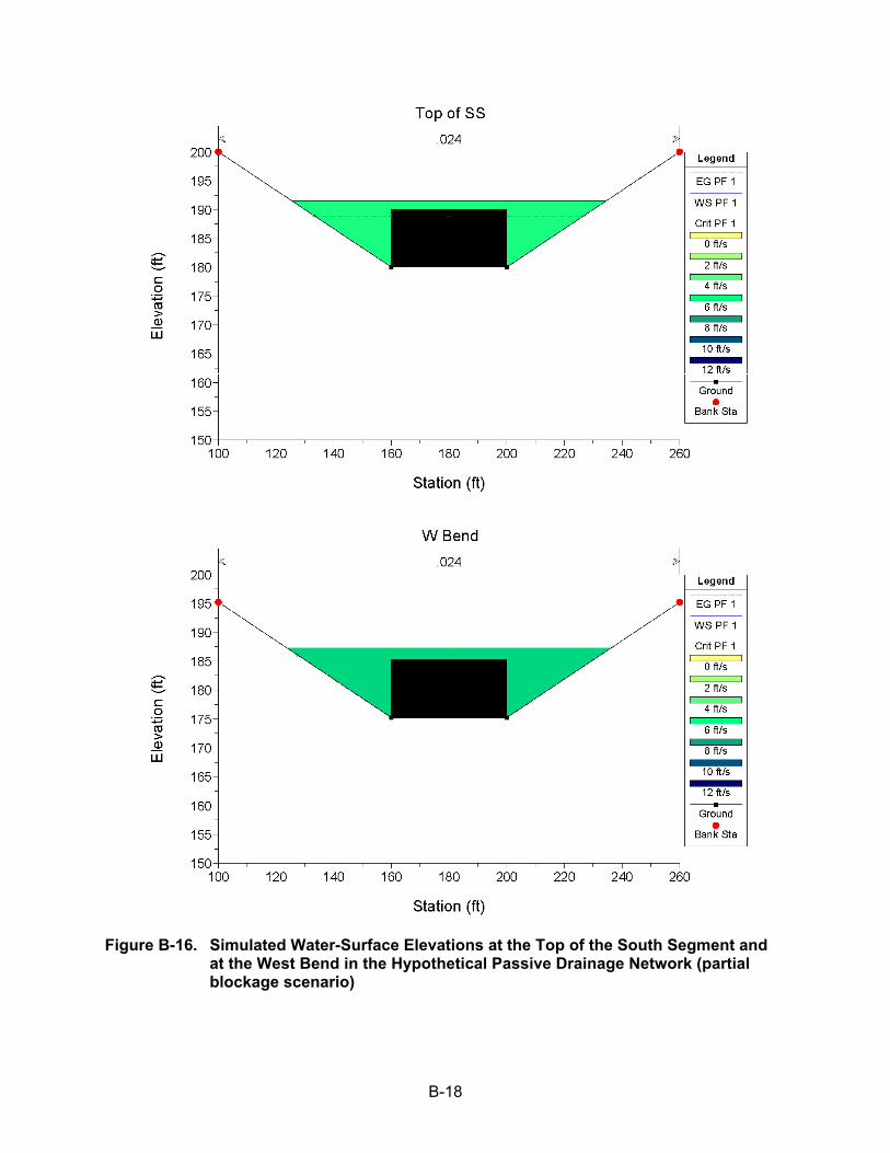
B-18
Figure B-16. Simulated Water-Surface Elevations at the Top of the South Segment and at the West Bend in the Hypothetical Passive Drainage Network (partial blockage scenario)
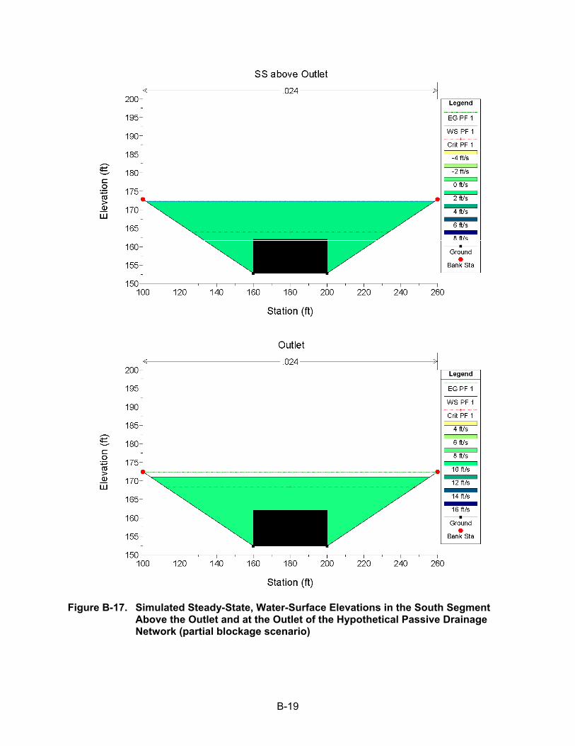
B-19
Figure B-17. Simulated Steady-State, Water-Surface Elevations in the South Segment Above the Outlet and at the Outlet of the Hypothetical Passive Drainage Network (partial blockage scenario)
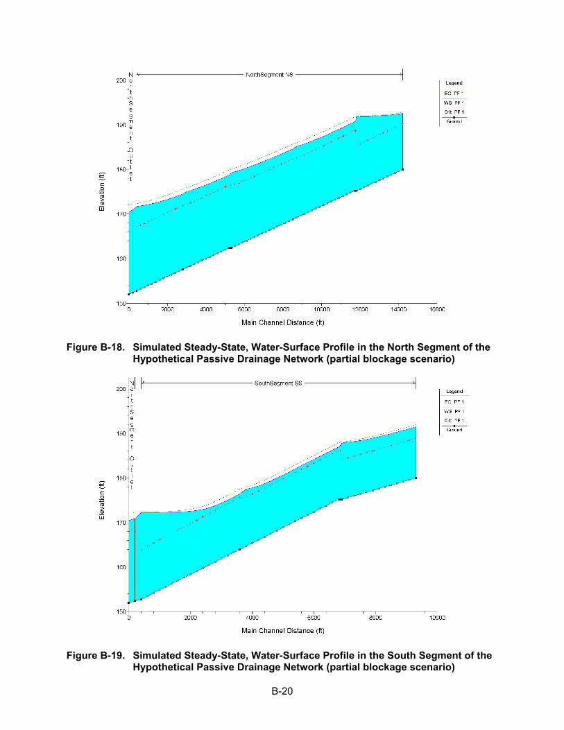
B-20
Figure B-18. Simulated Steady-State, Water-Surface Profile in the North Segment of the Hypothetical Passive Drainage Network (partial blockage scenario)
Figure B-19. Simulated Steady-State, Water-Surface Profile in the South Segment of the Hypothetical Passive Drainage Network (partial blockage scenario)
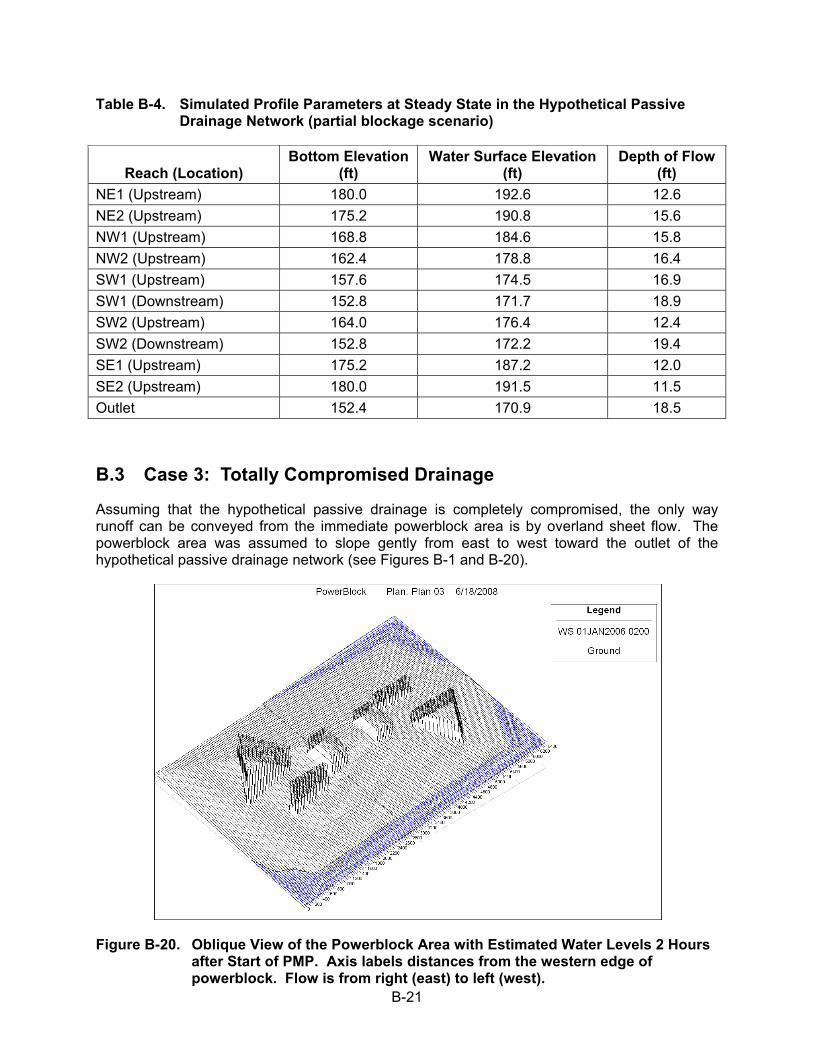
B-21
Table B-4. Simulated Profile Parameters at Steady State in the Hypothetical Passive Drainage Network (partial blockage scenario)
Reach (Location) Bottom Elevation
(ft) Water Surface Elevation
(ft) Depth of Flow
(ft)
NE1 (Upstream) 180.0 192.6 12.6
NE2 (Upstream) 175.2 190.8 15.6
NW1 (Upstream) 168.8 184.6 15.8
NW2 (Upstream) 162.4 178.8 16.4
SW1 (Upstream) 157.6 174.5 16.9
SW1 (Downstream) 152.8 171.7 18.9
SW2 (Upstream) 164.0 176.4 12.4
SW2 (Downstream) 152.8 172.2 19.4
SE1 (Upstream) 175.2 187.2 12.0
SE2 (Upstream) 180.0 191.5 11.5
Outlet 152.4 170.9 18.5
B.3 Case 3: Totally Compromised Drainage
Assuming that the hypothetical passive drainage is completely compromised, the only way runoff can be conveyed from the immediate powerblock area is by overland sheet flow. The powerblock area was assumed to slope gently from east to west toward the outlet of the hypothetical passive drainage network (see Figures B-1 and B-20).
Figure B-20. Oblique View of the Powerblock Area with Estimated Water Levels 2 Hours after Start of PMP. Axis labels distances from the western edge of powerblock. Flow is from right (east) to left (west).
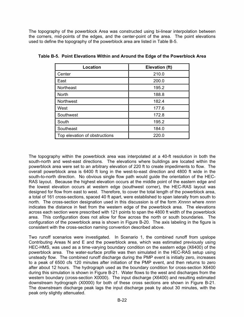
B-22
The topography of the powerblock Area was constructed using bi-linear interpolation between the corners, mid-points of the edges, and the center-point of the area. The point elevations used to define the topography of the powerblock area are listed in Table B-5.
Table B-5. Point Elevations Within and Around the Edge of the Powerblock Area
Location Elevation (ft)
Center 210.0
East 200.0
Northeast 195.2
North 188.8
Northwest 182.4
West 177.6
Southwest 172.8
South 195.2
Southeast 184.0
Top elevation of obstructions 220.0
The topography within the powerblock area was interpolated at a 40-ft resolution in both the south-north and west-east directions. The elevations where buildings are located within the powerblock area were set to an arbitrary elevation of 220 ft to create impediments to flow. The overall powerblock area is 6400 ft long in the west-to-east direction and 4800 ft wide in the south-to-north direction. No obvious single flow path would guide the orientation of the HEC-RAS layout. Because the highest elevation occurs at the middle point of the eastern edge and the lowest elevation occurs at western edge (southwest corner), the HEC-RAS layout was designed for flow from east to west. Therefore, to cover the total length of the powerblock area, a total of 161 cross-sections, spaced 40 ft apart, were established to span laterally from south to north. The cross-section designation used in this discussion is of the form Xnnnn where nnnn indicates the distance in feet from the western edge of the powerblock area. The elevations across each section were prescribed with 121 points to span the 4800 ft width of the powerblock area. This configuration does not allow for flow across the north or south boundaries. The configuration of the powerblock area is shown in Figure B-20. The axis labeling in the figure is consistent with the cross-section naming convention described above.
Two runoff scenarios were investigated. In Scenario 1, the combined runoff from upslope Contributing Areas N and E and the powerblock area, which was estimated previously using HEC-HMS, was used as a time-varying boundary condition on the eastern edge (X6400) of the powerblock area. The water-surface profile was then simulated in the HEC-RAS setup using unsteady flow. The combined runoff discharge during the PMP event is initially zero, increases to a peak of 6500 cfs 120 minutes after initiation of the PMP event, and then returns to zero after about 12 hours. The hydrograph used as the boundary condition for cross-section X6400 during this simulation is shown in Figure B-21. Water flows to the west and discharges from the western boundary (cross-section X0000). The input discharge (X6400) and resulting estimated downstream hydrograph (X0000) for both of these cross sections are shown in Figure B-21. The downstream discharge peak lags the input discharge peak by about 30 minutes, with the peak only slightly attenuated.
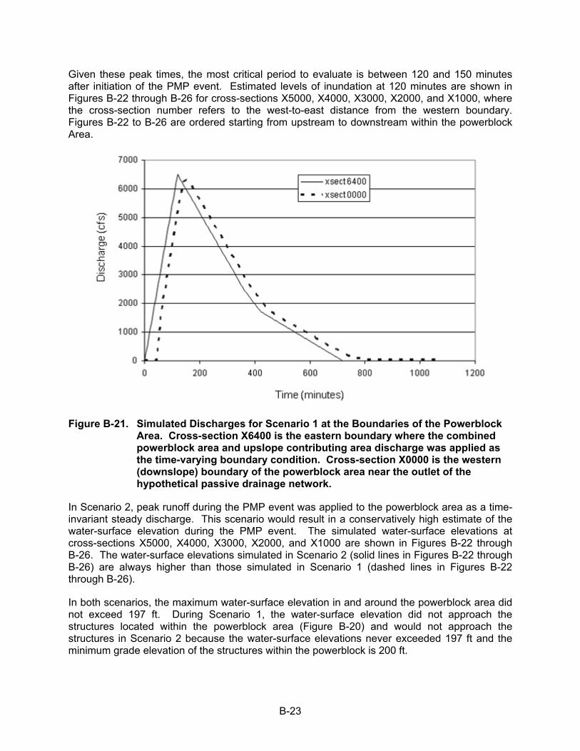
B-23
Given these peak times, the most critical period to evaluate is between 120 and 150 minutes after initiation of the PMP event. Estimated levels of inundation at 120 minutes are shown in Figures B-22 through B-26 for cross-sections X5000, X4000, X3000, X2000, and X1000, where the cross-section number refers to the west-to-east distance from the western boundary. Figures B-22 to B-26 are ordered starting from upstream to downstream within the powerblock Area.
Figure B-21. Simulated Discharges for Scenario 1 at the Boundaries of the Powerblock Area. Cross-section X6400 is the eastern boundary where the combined powerblock area and upslope contributing area discharge was applied as the time-varying boundary condition. Cross-section X0000 is the western (downslope) boundary of the powerblock area near the outlet of the hypothetical passive drainage network.
In Scenario 2, peak runoff during the PMP event was applied to the powerblock area as a time-invariant steady discharge. This scenario would result in a conservatively high estimate of the water-surface elevation during the PMP event. The simulated water-surface elevations at cross-sections X5000, X4000, X3000, X2000, and X1000 are shown in Figures B-22 through B-26. The water-surface elevations simulated in Scenario 2 (solid lines in Figures B-22 through B-26) are always higher than those simulated in Scenario 1 (dashed lines in Figures B-22 through B-26).
In both scenarios, the maximum water-surface elevation in and around the powerblock area did not exceed 197 ft. During Scenario 1, the water-surface elevation did not approach the structures located within the powerblock area (Figure B-20) and would not approach the structures in Scenario 2 because the water-surface elevations never exceeded 197 ft and the minimum grade elevation of the structures within the powerblock is 200 ft.
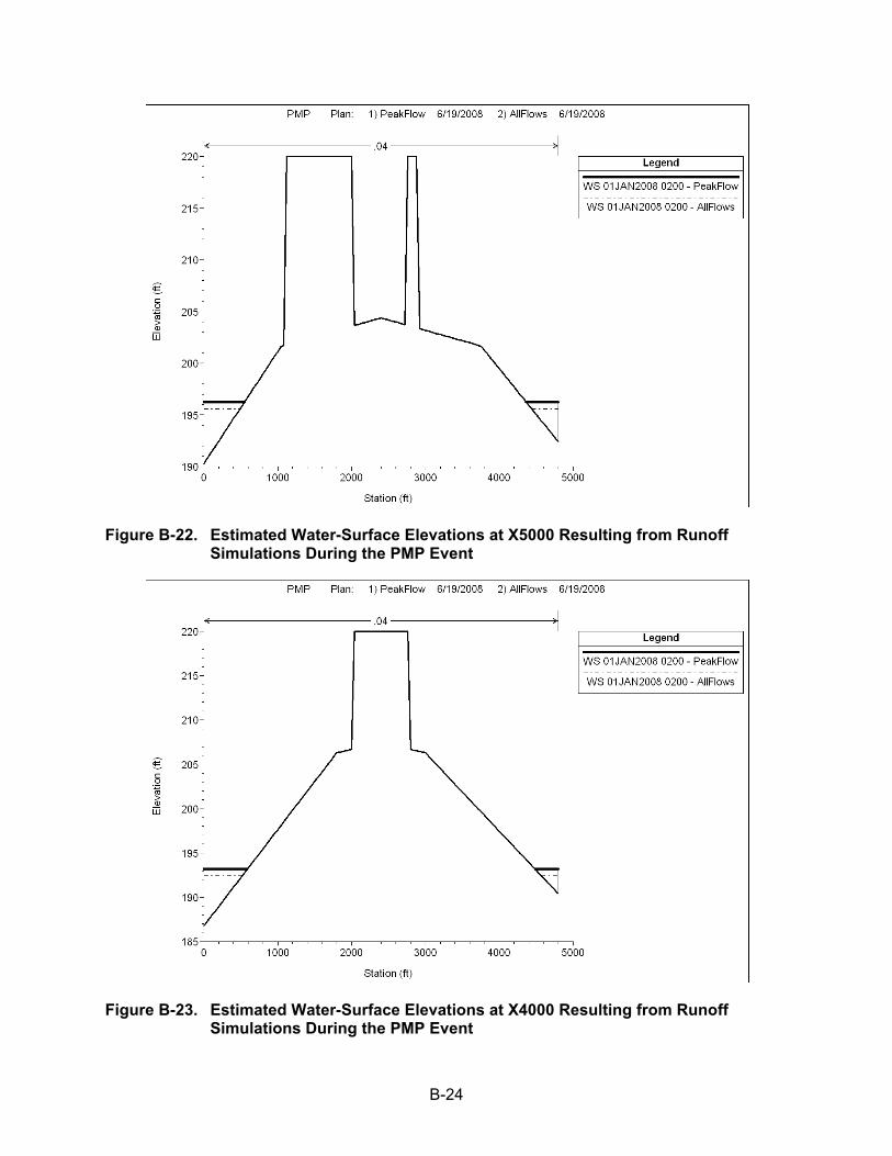
B-24
Figure B-22. Estimated Water-Surface Elevations at X5000 Resulting from Runoff Simulations During the PMP Event
Figure B-23. Estimated Water-Surface Elevations at X4000 Resulting from Runoff Simulations During the PMP Event
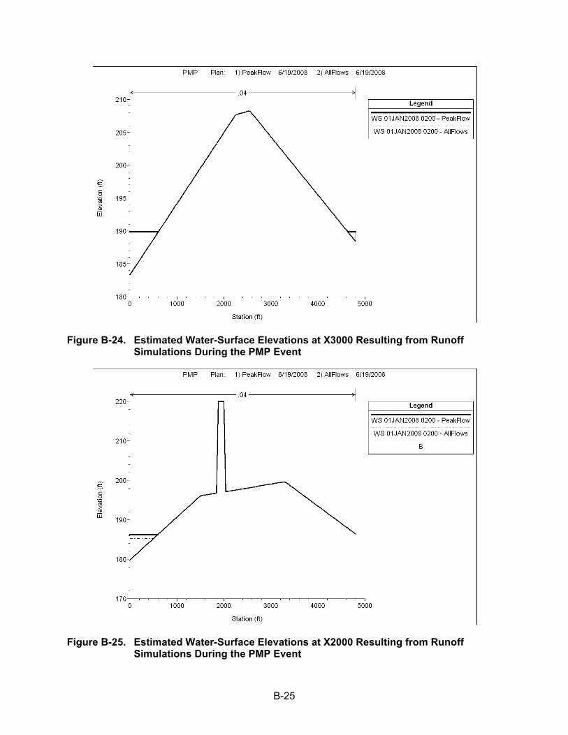
B-25
Figure B-24. Estimated Water-Surface Elevations at X3000 Resulting from Runoff Simulations During the PMP Event
Figure B-25. Estimated Water-Surface Elevations at X2000 Resulting from Runoff Simulations During the PMP Event
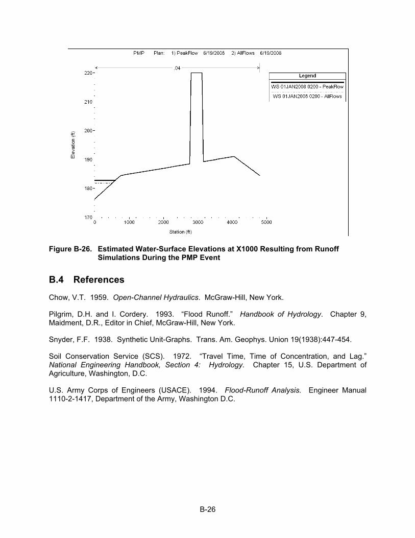
B-26
Figure B-26. Estimated Water-Surface Elevations at X1000 Resulting from Runoff Simulations During the PMP Event
B.4 References
Chow, V.T. 1959. Open-Channel Hydraulics. McGraw-Hill, New York.
Pilgrim, D.H. and I. Cordery. 1993. “Flood Runoff.” Handbook of Hydrology. Chapter 9, Maidment, D.R., Editor in Chief, McGraw-Hill, New York.
Snyder, F.F. 1938. Synthetic Unit-Graphs. Trans. Am. Geophys. Union 19(1938):447-454.
Soil Conservation Service (SCS). 1972. “Travel Time, Time of Concentration, and Lag.” National Engineering Handbook, Section 4: Hydrology. Chapter 15, U.S. Department of Agriculture, Washington, D.C.
U.S. Army Corps of Engineers (USACE). 1994. Flood-Runoff Analysis. Engineer Manual 1110-2-1417, Department of the Army, Washington D.C.
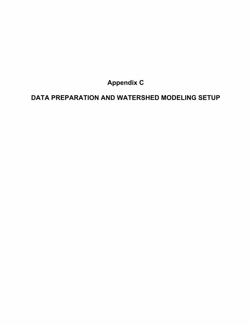
Appendix C
DATA PREPARATION AND WATERSHED MODELING SETUP


C-1
APPENDIX C
DATA PREPARATION AND WATERSHED MODELING SETUP
This appendix describes the procedures used to prepare hydrological data and set up a watershed model to estimate design basis flood events that then can be used for design criteria at a proposed nuclear power plant site. The software used in this case study includes the Environmental Systems Research Institute’s (ESRI’s) ArcGIS v. 9.2, Environmental Modeling Systems, Inc.’s Watershed Modeling System (WMS) Volume 8.0, and U.S. Army Corps of Engineers’s Hydrologic Engineering Center Hydrologic Modeling System (HEC-HMS) 3.2.
In the following subsections, we describe hydrologic data preparation, delineation and setup of the watershed in WMS, and estimation of the probable maximum precipitation (PMP), probable maximum flood (PMF), and PMF water-surface elevations.
C.1 Digital Elevation Model Data Preparation
C.1.1 Compiling the Digital Elevation Models
The first step in the data-preparation process involved compiling the 8-digit level Hydrologic Unit Code (HUC) boundaries for the drainage area of interest and subsequently identifying and collecting source Digital Elevation Models (DEMs) (described elsewhere in this document). For this case study, National Elevation Dataset (NED) DEM data at a 30-m resolution were collected for the study site. Normally, 10-m DEM data are desired as a starting point for data assembly because they provide the highest-level of resolution and accuracy, can be re-sampled to a desired and manageable resolution for large watersheds, and can still be available for finer-scale modeling work if necessary. The disadvantage of using 10-m DEM data is that their size can be burdensome for larger watersheds; however, frequently the effort is worthwhile because it allows subsequent work to be based on the same underlying terrain model. For this study site, 30-m DEM data were selected because 10-m data were not available for all areas within the domain.
A DEM resolution of 180 m was deemed suitable for demonstrating the methodology. The approximately 3000-mi2 watershed was modeled using approximately 670,000 computational grid cells. The individual DEM tiles downloaded from the U.S. Geological Survey (USGS) (http://seamless.usgs.gov/) were mosaicked, cleaned, and re-sampled using ArcGIS v.9.2. While WMS provides the capability to do this preparatory work, it has been found to be more effective to assemble DEM data in ArcGIS and then to present a model-ready DEM to WMS. It also should be noted that a beta-version of USACE’s HEC-GeoHMS for ArcGIS software was evaluated for this study and was determined to be not yet suitable for production work. However, it is expected that in the future, GeoHMS for ArcGIS may become the accepted standard for preparing spatial data for HEC-HMS modeling.
Within ArcGIS, individual DEM tiles were loaded, and the ‘Mosaic to New Raster’ toolbox utility, which requires an ArcGIS Spatial Analyst license, was used to bring the terrain model into a single dataset. To prepare the DEM data for hydrologic modeling, the Center for Research in Water Resources, University of Texas at Austin’s free ArcHydro v. 1.3 ArcGIS toolbox was used.
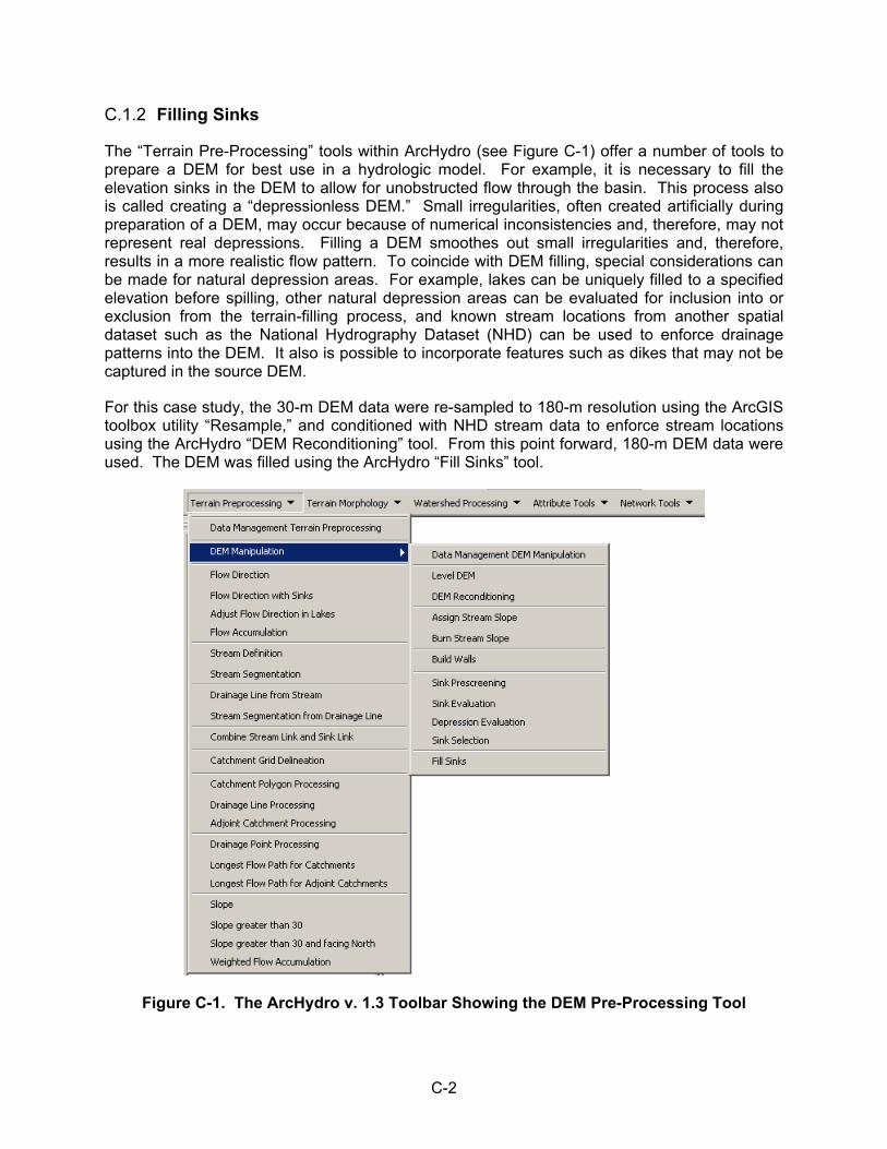
C-2
C.1.2 Filling Sinks
The “Terrain Pre-Processing” tools within ArcHydro (see Figure C-1) offer a number of tools to prepare a DEM for best use in a hydrologic model. For example, it is necessary to fill the elevation sinks in the DEM to allow for unobstructed flow through the basin. This process also is called creating a “depressionless DEM.” Small irregularities, often created artificially during preparation of a DEM, may occur because of numerical inconsistencies and, therefore, may not represent real depressions. Filling a DEM smoothes out small irregularities and, therefore, results in a more realistic flow pattern. To coincide with DEM filling, special considerations can be made for natural depression areas. For example, lakes can be uniquely filled to a specified elevation before spilling, other natural depression areas can be evaluated for inclusion into or exclusion from the terrain-filling process, and known stream locations from another spatial dataset such as the National Hydrography Dataset (NHD) can be used to enforce drainage patterns into the DEM. It also is possible to incorporate features such as dikes that may not be captured in the source DEM.
For this case study, the 30-m DEM data were re-sampled to 180-m resolution using the ArcGIS toolbox utility “Resample,” and conditioned with NHD stream data to enforce stream locations using the ArcHydro “DEM Reconditioning” tool. From this point forward, 180-m DEM data were used. The DEM was filled using the ArcHydro “Fill Sinks” tool.
Figure C-1. The ArcHydro v. 1.3 Toolbar Showing the DEM Pre-Processing Tool
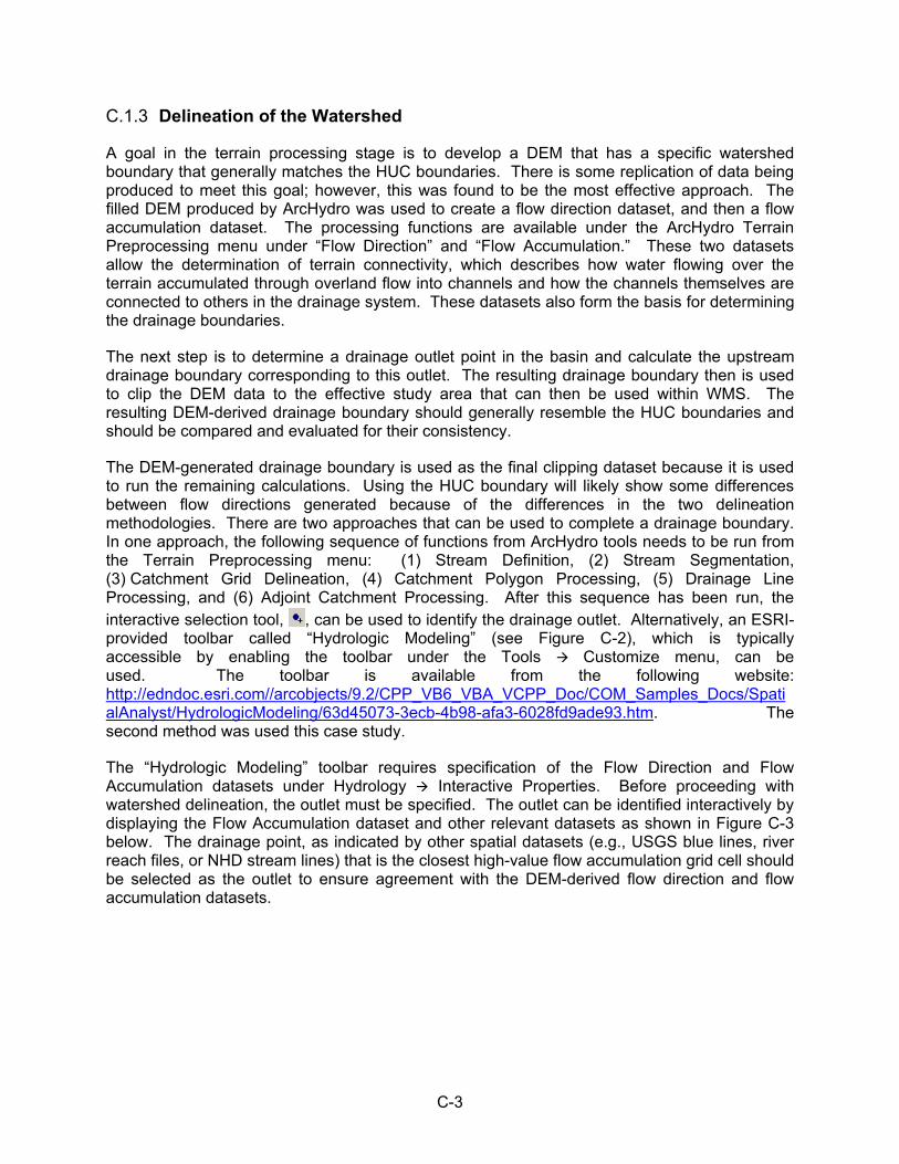
C-3
C.1.3 Delineation of the Watershed
A goal in the terrain processing stage is to develop a DEM that has a specific watershed boundary that generally matches the HUC boundaries. There is some replication of data being produced to meet this goal; however, this was found to be the most effective approach. The filled DEM produced by ArcHydro was used to create a flow direction dataset, and then a flow accumulation dataset. The processing functions are available under the ArcHydro Terrain Preprocessing menu under “Flow Direction” and “Flow Accumulation.” These two datasets allow the determination of terrain connectivity, which describes how water flowing over the terrain accumulated through overland flow into channels and how the channels themselves are connected to others in the drainage system. These datasets also form the basis for determining the drainage boundaries.
The next step is to determine a drainage outlet point in the basin and calculate the upstream drainage boundary corresponding to this outlet. The resulting drainage boundary then is used to clip the DEM data to the effective study area that can then be used within WMS. The resulting DEM-derived drainage boundary should generally resemble the HUC boundaries and should be compared and evaluated for their consistency.
The DEM-generated drainage boundary is used as the final clipping dataset because it is used to run the remaining calculations. Using the HUC boundary will likely show some differences between flow directions generated because of the differences in the two delineation methodologies. There are two approaches that can be used to complete a drainage boundary. In one approach, the following sequence of functions from ArcHydro tools needs to be run from the Terrain Preprocessing menu: (1) Stream Definition, (2) Stream Segmentation, (3) Catchment Grid Delineation, (4) Catchment Polygon Processing, (5) Drainage Line Processing, and (6) Adjoint Catchment Processing. After this sequence has been run, the interactive selection tool, , can be used to identify the drainage outlet. Alternatively, an ESRI-provided toolbar called “Hydrologic Modeling” (see Figure C-2), which is typically accessible by enabling the toolbar under the Tools Customize menu, can be used. The toolbar is available from the following website: http://edndoc.esri.com//arcobjects/9.2/CPP_VB6_VBA_VCPP_Doc/COM_Samples_Docs/SpatialAnalyst/HydrologicModeling/63d45073-3ecb-4b98-afa3-6028fd9ade93.htm. The second method was used this case study.
The “Hydrologic Modeling” toolbar requires specification of the Flow Direction and Flow Accumulation datasets under Hydrology Interactive Properties. Before proceeding with watershed delineation, the outlet must be specified. The outlet can be identified interactively by displaying the Flow Accumulation dataset and other relevant datasets as shown in Figure C-3 below. The drainage point, as indicated by other spatial datasets (e.g., USGS blue lines, river reach files, or NHD stream lines) that is the closest high-value flow accumulation grid cell should be selected as the outlet to ensure agreement with the DEM-derived flow direction and flow accumulation datasets.
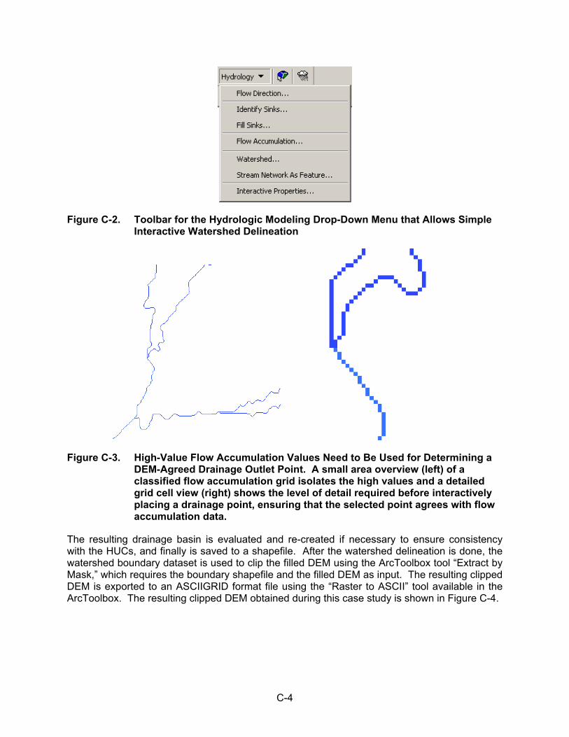
C-4
Figure C-2. Toolbar for the Hydrologic Modeling Drop-Down Menu that Allows Simple Interactive Watershed Delineation
Figure C-3. High-Value Flow Accumulation Values Need to Be Used for Determining a DEM-Agreed Drainage Outlet Point. A small area overview (left) of a classified flow accumulation grid isolates the high values and a detailed grid cell view (right) shows the level of detail required before interactively placing a drainage point, ensuring that the selected point agrees with flow accumulation data.
The resulting drainage basin is evaluated and re-created if necessary to ensure consistency with the HUCs, and finally is saved to a shapefile. After the watershed delineation is done, the watershed boundary dataset is used to clip the filled DEM using the ArcToolbox tool “Extract by Mask,” which requires the boundary shapefile and the filled DEM as input. The resulting clipped DEM is exported to an ASCIIGRID format file using the “Raster to ASCII” tool available in the ArcToolbox. The resulting clipped DEM obtained during this case study is shown in Figure C-4.
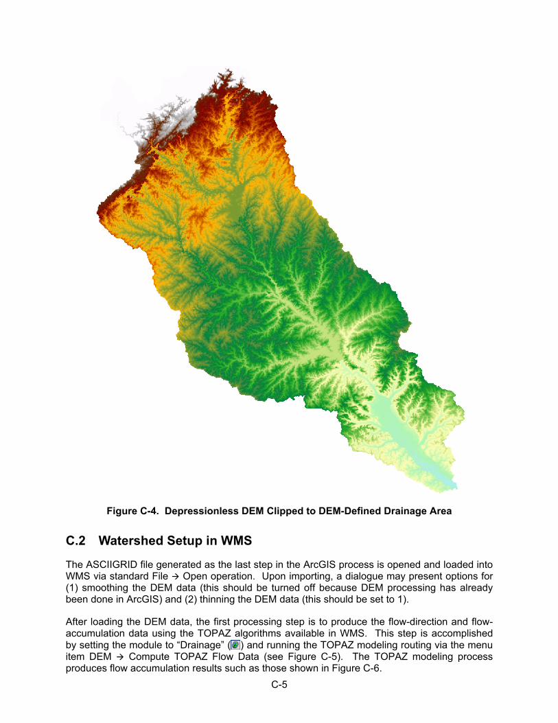
C-5
Figure C-4. Depressionless DEM Clipped to DEM-Defined Drainage Area
C.2 Watershed Setup in WMS
The ASCIIGRID file generated as the last step in the ArcGIS process is opened and loaded into WMS via standard File Open operation. Upon importing, a dialogue may present options for (1) smoothing the DEM data (this should be turned off because DEM processing has already been done in ArcGIS) and (2) thinning the DEM data (this should be set to 1).
After loading the DEM data, the first processing step is to produce the flow-direction and flow-accumulation data using the TOPAZ algorithms available in WMS. This step is accomplished by setting the module to “Drainage” ( ) and running the TOPAZ modeling routing via the menu item DEM Compute TOPAZ Flow Data (see Figure C-5). The TOPAZ modeling process produces flow accumulation results such as those shown in Figure C-6.
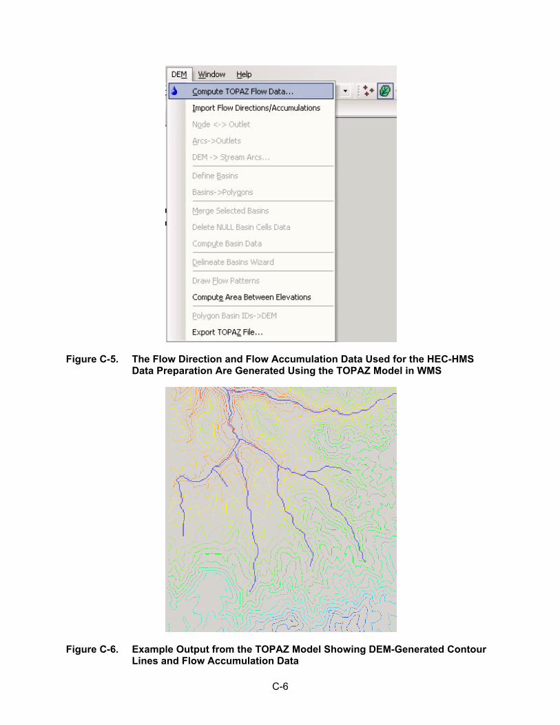
C-6
Figure C-5. The Flow Direction and Flow Accumulation Data Used for the HEC-HMS Data Preparation Are Generated Using the TOPAZ Model in WMS
Figure C-6. Example Output from the TOPAZ Model Showing DEM-Generated Contour Lines and Flow Accumulation Data

C-7
As was demonstrated in the ArcGIS processing, once the flow-direction and flow-accumulation data are generated, a watershed boundary can be delineated. This process is accomplished in two steps. First the overall drainage area is delineated, and then the sub-basins are defined within the overall drainage area. The farthest downstream point in the watershed will define the extent of the watershed boundary. In WMS, this point is indicated by zooming into the grid-cell
level, using the “Create Outlet Point” button ( ), and ensuring this location falls upon one of the flow accumulation cell points, similar to the operation conducted in ArcGIS. Once the drainage outlet is defined, the following commands are executed from the WMS menu:
DEM Stream Arcs
DEM Define Basins
DEM Basins Polygons
DEM Compute Basin Data.
For a large watershed, these processes may be computationally intensive.
The case-study watershed was broken into 13 subbasin areas and was created by additional outlet points in WMS. Within the “Drainage” module, the “Select Feature Vertex” tool ( ) is used to identify the sub-basin outlets. The feature vertex is selected as shown in Figure C-7, and is converted to an outlet using the DEM Node Vertex menu option. The process is repeated for all 13 subbasins. When completed, the subbasins are defined, and statistics may be computed by executing the following sequence:
DEM Define Basins
DEM Basins Polygons
DEM Compute Basin Data.
The WMS sub-basin delineations for the case-study basin are presented in Figure C-8 and Figure C-9.
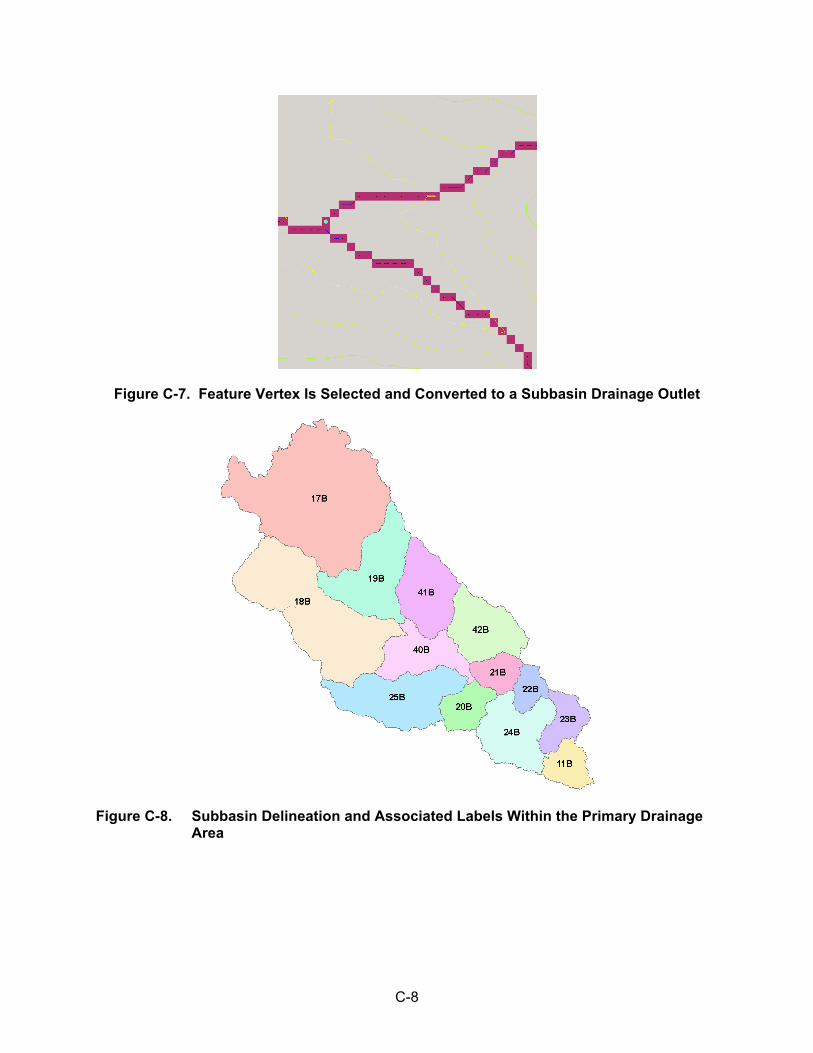
C-8
Figure C-7. Feature Vertex Is Selected and Converted to a Subbasin Drainage Outlet
Figure C-8. Subbasin Delineation and Associated Labels Within the Primary Drainage Area
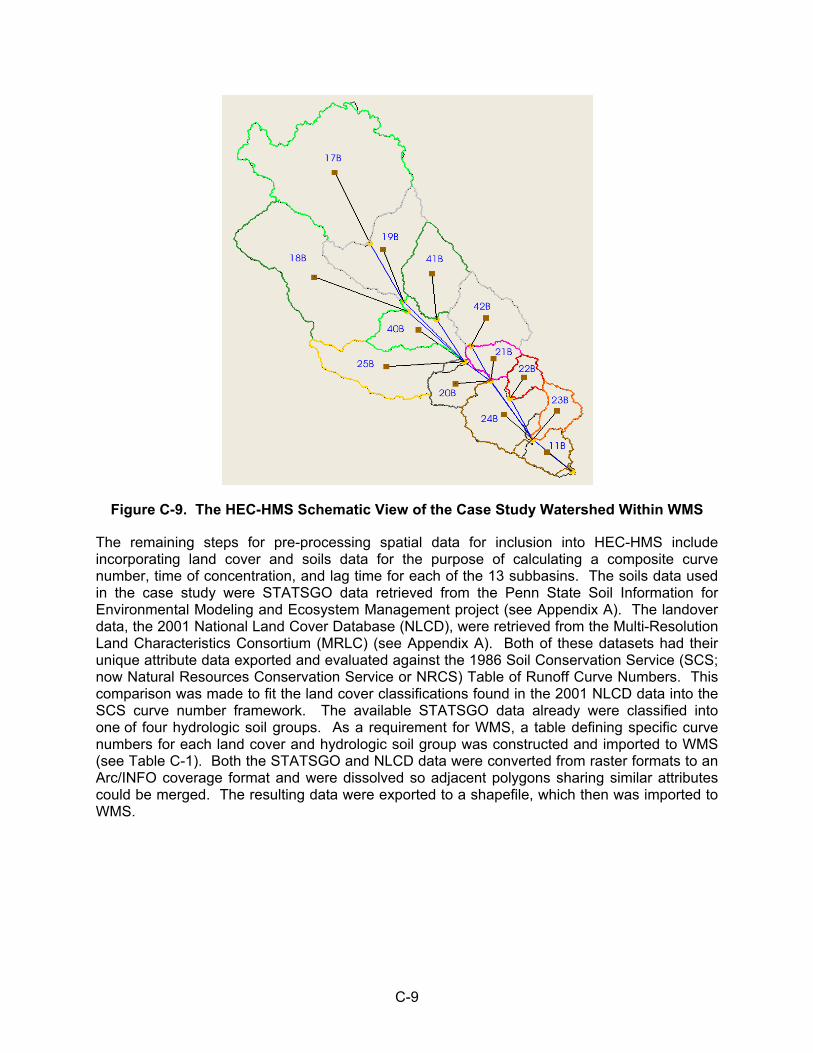
C-9
Figure C-9. The HEC-HMS Schematic View of the Case Study Watershed Within WMS
The remaining steps for pre-processing spatial data for inclusion into HEC-HMS include incorporating land cover and soils data for the purpose of calculating a composite curve number, time of concentration, and lag time for each of the 13 subbasins. The soils data used in the case study were STATSGO data retrieved from the Penn State Soil Information for Environmental Modeling and Ecosystem Management project (see Appendix A). The landover data, the 2001 National Land Cover Database (NLCD), were retrieved from the Multi-Resolution Land Characteristics Consortium (MRLC) (see Appendix A). Both of these datasets had their unique attribute data exported and evaluated against the 1986 Soil Conservation Service (SCS; now Natural Resources Conservation Service or NRCS) Table of Runoff Curve Numbers. This comparison was made to fit the land cover classifications found in the 2001 NLCD data into the SCS curve number framework. The available STATSGO data already were classified into one of four hydrologic soil groups. As a requirement for WMS, a table defining specific curve numbers for each land cover and hydrologic soil group was constructed and imported to WMS (see Table C-1). Both the STATSGO and NLCD data were converted from raster formats to an Arc/INFO coverage format and were dissolved so adjacent polygons sharing similar attributes could be merged. The resulting data were exported to a shapefile, which then was imported to WMS.
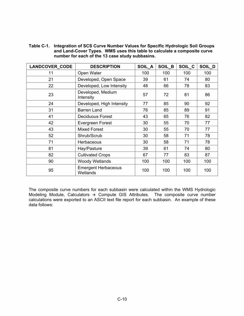
C-10
Table C-1. Integration of SCS Curve Number Values for Specific Hydrologic Soil Groups and Land-Cover Types. WMS uses this table to calculate a composite curve number for each of the 13 case study subbasins.
LANDCOVER_CODE DESCRIPTION SOIL_A SOIL_B SOIL_C SOIL_D
11 Open Water 100 100 100 100
21 Developed, Open Space 39 61 74 80
22 Developed, Low Intensity 48 66 78 83
23 Developed, Medium Intensity
57 72 81 86
24 Developed, High Intensity 77 85 90 92
31 Barren Land 76 85 89 91
41 Deciduous Forest 43 65 76 82
42 Evergreen Forest 30 55 70 77
43 Mixed Forest 30 55 70 77
52 Shrub/Scrub 30 58 71 78
71 Herbaceous 30 58 71 78
81 Hay/Pasture 39 61 74 80
82 Cultivated Crops 67 77 83 87
90 Woody Wetlands 100 100 100 100
95 Emergent Herbaceous Wetlands
100 100 100 100
The composite curve numbers for each subbasin were calculated within the WMS Hydrologic Modeling Module, Calculators Compute GIS Attributes. The composite curve number calculations were exported to an ASCII text file report for each subbasin. An example of these data follows:
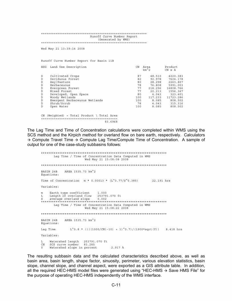
C-11
========================================================== Runoff Curve Number Report (Generated by WMS) ========================================================== Wed May 21 13:39:14 2008 Runoff Curve Number Report for Basin 11B HSG Land Use Description CN Area Product km^2 CN x A D Cultivated Crops 87 48.510 4220.383 D Deciduous Forest 82 92.978 7624.178 D Hay/Pasture 80 28.298 2263.807 D Herbaceuous 78 76.808 5991.003 D Evergreen Forest 77 218.296 16808.766 D Mixed Forest 77 20.213 1556.367 D Developed, Open Space 80 4.043 323.401 D Woody Wetlands 100 117.233 11723.286 D Emergent Herbaceuous Wetlands 100 8.085 808.502 D Shrub/Scrub 78 4.043 315.316 D Open Water 100 8.085 808.502 CN (Weighted) = Total Product \ Total Area ========================================== 83.6968
The Lag Time and Time of Concentration calculations were completed within WMS using the SCS method and the Kirpich method for overland flow on bare earth, respectively. Calculators Compute Travel Time Compute Lag Time/Compute Time of Concentration. A sample of output for one of the case-study subbasins follows:
********************************************************************* Lag Time / Time of Concentration Data Computed in WMS Wed May 21 15:08:08 2008 ********************************************************************* BASIN 24B AREA 1535.73 km^2 Equations: Time of Concentration m * 0.00013 * (L^0.77/S^0.385) 22.191 hrs Variables: m Earth type coefficient 1.000 L Length of overland flow 253791.070 ft S average overland slope 0.002 ********************************************************************* Lag Time / Time of Concentration Data Computed in WMS Wed May 21 15:08:22 2008 ********************************************************************* BASIN 24B AREA 1535.73 km^2 Equations: Lag Time L^0.8 * ((((1000/CN)-10) + 1)^0.7)/(1900*sqrt(Y)) 8.418 hrs Variables: L Watershed length 253791.070 ft CN SCS curve number 83.285 Y Watershed slope in percent 2.917 %
The resulting subbasin data and the calculated characteristics described above, as well as basin area, basin length, shape factor, sinuosity, perimeter, various elevation statistics, basin slope, channel slope, and channel aspect, were exported as a GIS attribute table. In addition, all the required HEC-HMS model files were generated using “HEC-HMS Save HMS File” for the purpose of operating HEC-HMS independently of the WMS interface.
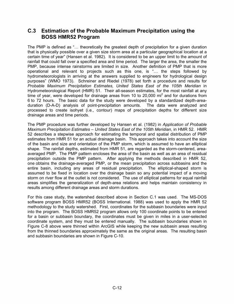
C-12
C.3 Estimation of the Probable Maximum Precipitation using the BOSS HMR52 Program
The PMP is defined as “… theoretically the greatest depth of precipitation for a given duration that is physically possible over a given size storm area at a particular geographical location at a certain time of year” (Hansen et al. 1982). It is considered to be an upper limit to the amount of rainfall that could fall over a specified area and time period. The larger the area, the smaller the PMP, because intense rainstorms are limited in size. Another definition of PMP that is more operational and relevant to projects such as this one, is “… the steps followed by hydrometeorologists in arriving at the answers supplied to engineers for hydrological design purposes” (WMO 1973). Schreiner and Riedel (1978) set forth a procedure and results for Probable Maximum Precipitation Estimates, United States East of the 105th Meridian in Hydrometeorological Report (HMR) 51. Their all-season estimates, for the most rainfall at any time of year, were developed for drainage areas from 10 to 20,000 mi2 and for durations from 6 to 72 hours. The basic data for the study were developed by a standardized depth-area-duration (D-A-D) analysis of point-precipitation amounts. The data were analyzed and processed to create isohyet (i.e., contour) maps of precipitation depths for different size drainage areas and time periods.
The PMP procedure was further developed by Hansen et al. (1982) in Application of Probable Maximum Precipitation Estimates – United States East of the 105th Meridian, in HMR 52. HMR 52 describes a stepwise approach for estimating the temporal and spatial distribution of PMP estimates from HMR 51 for an actual drainage basin. This approach takes into account the size of the basin and size and orientation of the PMP storm, which is assumed to have an elliptical shape. The rainfall depths, estimated from HMR 51, are regarded as the storm-centered, area-averaged PMP. The PMP pattern encloses the area of the basin as well as an area of residual precipitation outside the PMP pattern. After applying the methods described in HMR 52, one obtains the drainage-averaged PMP, or the mean precipitation across subbasins and the entire basin, including any areas of residual precipitation. The elliptical-shaped storm is assumed to be fixed in location over the drainage basin so any potential impact of a moving storm on river flow at the outlet is not considered. The use of elliptical patterns for equal rainfall areas simplifies the generalization of depth-area relations and helps maintain consistency in results among different drainage areas and storm durations.
For this case study, the watershed described above in Section C.1 was used. The MS-DOS software program BOSS HMR52 (BOSS International. 1988) was used to apply the HMR 52 methodology to the study watershed. First, coordinates for the subbasin boundaries were input into the program. The BOSS HMR52 program allows only 100 coordinate points to be entered for a basin or subbasin boundary, the coordinates must be given in miles in a user-selected coordinate system, and they must be entered manually. The subbasin boundaries shown in Figure C-8 above were thinned within ArcGIS while keeping the new subbasin areas resulting from the thinned boundaries approximately the same as the original areas. The resulting basin and subbasin boundaries are shown in Figure C-10.
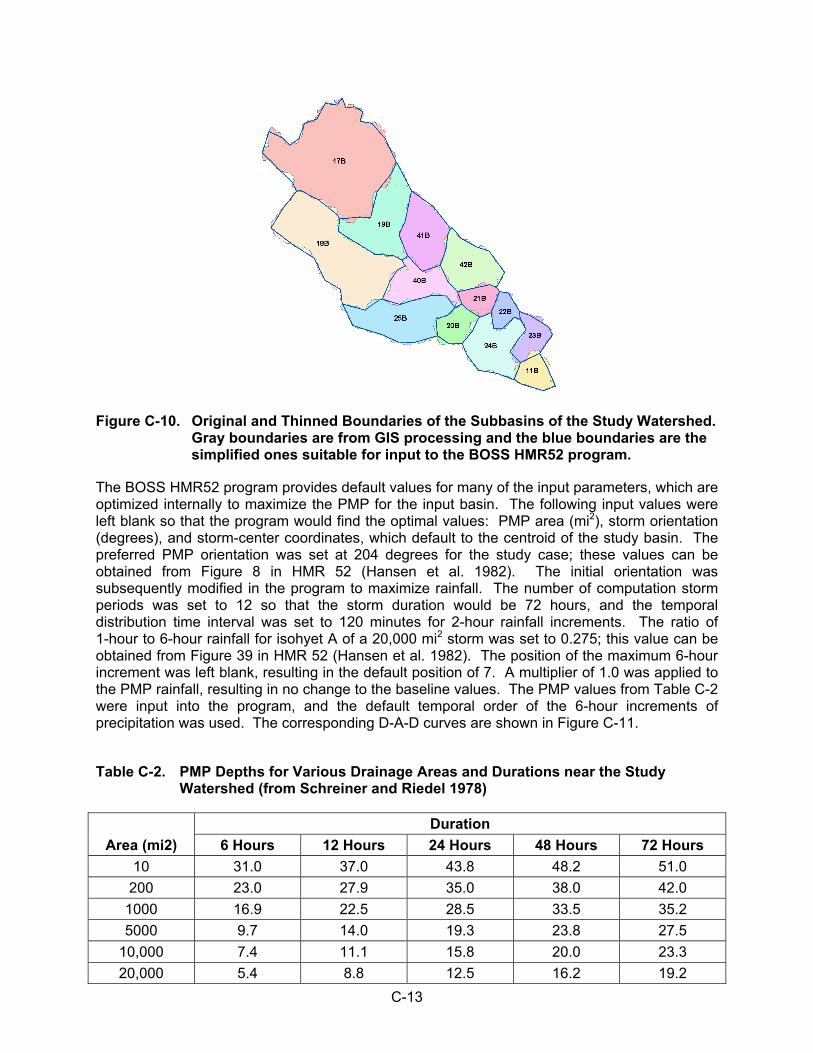
C-13
Figure C-10. Original and Thinned Boundaries of the Subbasins of the Study Watershed. Gray boundaries are from GIS processing and the blue boundaries are the simplified ones suitable for input to the BOSS HMR52 program.
The BOSS HMR52 program provides default values for many of the input parameters, which are optimized internally to maximize the PMP for the input basin. The following input values were left blank so that the program would find the optimal values: PMP area (mi2), storm orientation (degrees), and storm-center coordinates, which default to the centroid of the study basin. The preferred PMP orientation was set at 204 degrees for the study case; these values can be obtained from Figure 8 in HMR 52 (Hansen et al. 1982). The initial orientation was subsequently modified in the program to maximize rainfall. The number of computation storm periods was set to 12 so that the storm duration would be 72 hours, and the temporal distribution time interval was set to 120 minutes for 2-hour rainfall increments. The ratio of 1-hour to 6-hour rainfall for isohyet A of a 20,000 mi2 storm was set to 0.275; this value can be obtained from Figure 39 in HMR 52 (Hansen et al. 1982). The position of the maximum 6-hour increment was left blank, resulting in the default position of 7. A multiplier of 1.0 was applied to the PMP rainfall, resulting in no change to the baseline values. The PMP values from Table C-2 were input into the program, and the default temporal order of the 6-hour increments of precipitation was used. The corresponding D-A-D curves are shown in Figure C-11.
Table C-2. PMP Depths for Various Drainage Areas and Durations near the Study Watershed (from Schreiner and Riedel 1978)
Area (mi2)
Duration
6 Hours 12 Hours 24 Hours 48 Hours 72 Hours
10 31.0 37.0 43.8 48.2 51.0
200 23.0 27.9 35.0 38.0 42.0
1000 16.9 22.5 28.5 33.5 35.2
5000 9.7 14.0 19.3 23.8 27.5
10,000 7.4 11.1 15.8 20.0 23.3
20,000 5.4 8.8 12.5 16.2 19.2
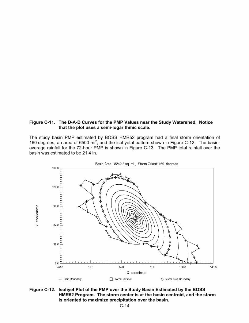
C-14
Figure C-11. The D-A-D Curves for the PMP Values near the Study Watershed. Notice that the plot uses a semi-logarithmic scale.
The study basin PMP estimated by BOSS HMR52 program had a final storm orientation of 160 degrees, an area of 6500 mi2, and the isohyetal pattern shown in Figure C-12. The basin-average rainfall for the 72-hour PMP is shown in Figure C-13. The PMP total rainfall over the basin was estimated to be 21.4 in.
Figure C-12. Isohyet Plot of the PMP over the Study Basin Estimated by the BOSS HMR52 Program. The storm center is at the basin centroid, and the storm is oriented to maximize precipitation over the basin.
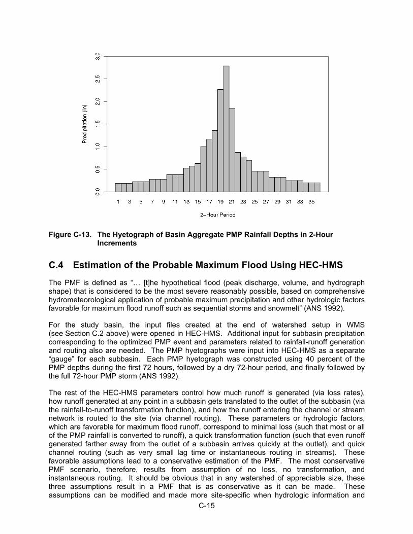
C-15
Figure C-13. The Hyetograph of Basin Aggregate PMP Rainfall Depths in 2-Hour Increments
C.4 Estimation of the Probable Maximum Flood Using HEC-HMS
The PMF is defined as “… [t]he hypothetical flood (peak discharge, volume, and hydrograph shape) that is considered to be the most severe reasonably possible, based on comprehensive hydrometeorological application of probable maximum precipitation and other hydrologic factors favorable for maximum flood runoff such as sequential storms and snowmelt” (ANS 1992).
For the study basin, the input files created at the end of watershed setup in WMS (see Section C.2 above) were opened in HEC-HMS. Additional input for subbasin precipitation corresponding to the optimized PMP event and parameters related to rainfall-runoff generation and routing also are needed. The PMP hyetographs were input into HEC-HMS as a separate “gauge” for each subbasin. Each PMP hyetograph was constructed using 40 percent of the PMP depths during the first 72 hours, followed by a dry 72-hour period, and finally followed by the full 72-hour PMP storm (ANS 1992).
The rest of the HEC-HMS parameters control how much runoff is generated (via loss rates), how runoff generated at any point in a subbasin gets translated to the outlet of the subbasin (via the rainfall-to-runoff transformation function), and how the runoff entering the channel or stream network is routed to the site (via channel routing). These parameters or hydrologic factors, which are favorable for maximum flood runoff, correspond to minimal loss (such that most or all of the PMP rainfall is converted to runoff), a quick transformation function (such that even runoff generated farther away from the outlet of a subbasin arrives quickly at the outlet), and quick channel routing (such as very small lag time or instantaneous routing in streams). These favorable assumptions lead to a conservative estimation of the PMF. The most conservative PMF scenario, therefore, results from assumption of no loss, no transformation, and instantaneous routing. It should be obvious that in any watershed of appreciable size, these three assumptions result in a PMF that is as conservative as it can be made. These assumptions can be modified and made more site-specific when hydrologic information and
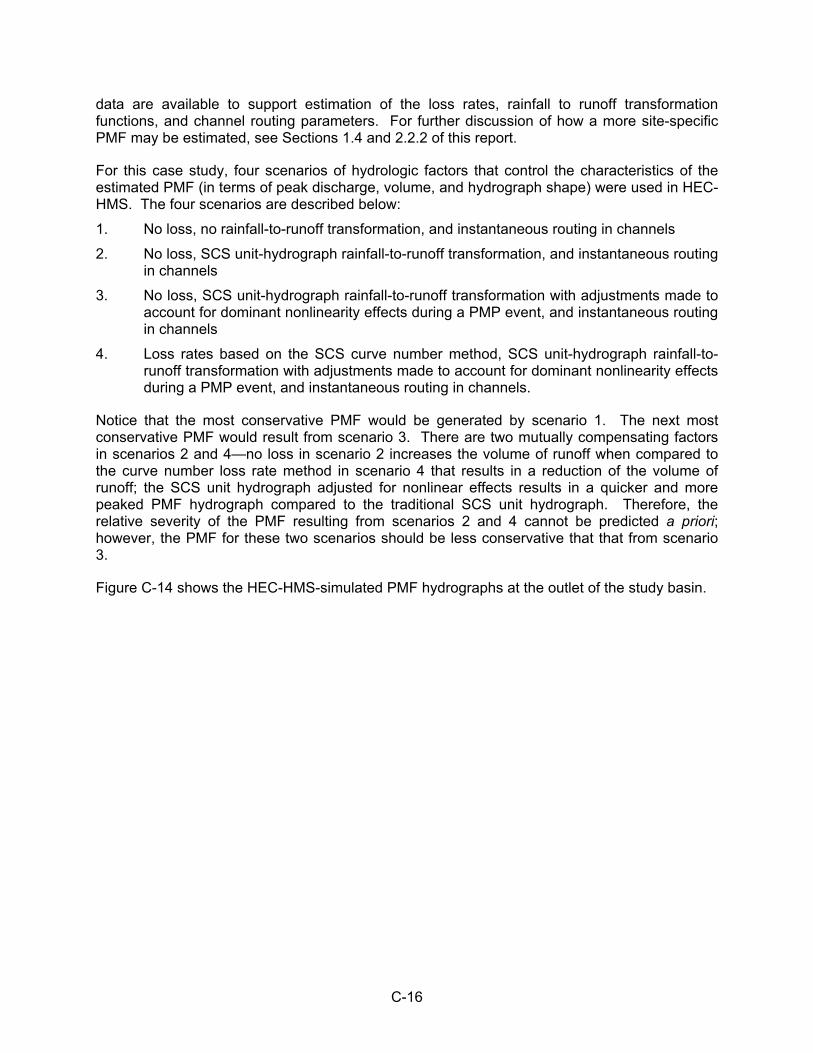
C-16
data are available to support estimation of the loss rates, rainfall to runoff transformation functions, and channel routing parameters. For further discussion of how a more site-specific PMF may be estimated, see Sections 1.4 and 2.2.2 of this report.
For this case study, four scenarios of hydrologic factors that control the characteristics of the estimated PMF (in terms of peak discharge, volume, and hydrograph shape) were used in HEC-HMS. The four scenarios are described below:
1. No loss, no rainfall-to-runoff transformation, and instantaneous routing in channels
2. No loss, SCS unit-hydrograph rainfall-to-runoff transformation, and instantaneous routing in channels
3. No loss, SCS unit-hydrograph rainfall-to-runoff transformation with adjustments made to account for dominant nonlinearity effects during a PMP event, and instantaneous routing in channels
4. Loss rates based on the SCS curve number method, SCS unit-hydrograph rainfall-to-runoff transformation with adjustments made to account for dominant nonlinearity effects during a PMP event, and instantaneous routing in channels.
Notice that the most conservative PMF would be generated by scenario 1. The next most conservative PMF would result from scenario 3. There are two mutually compensating factors in scenarios 2 and 4—no loss in scenario 2 increases the volume of runoff when compared to the curve number loss rate method in scenario 4 that results in a reduction of the volume of runoff; the SCS unit hydrograph adjusted for nonlinear effects results in a quicker and more peaked PMF hydrograph compared to the traditional SCS unit hydrograph. Therefore, the relative severity of the PMF resulting from scenarios 2 and 4 cannot be predicted a priori; however, the PMF for these two scenarios should be less conservative that that from scenario 3.
Figure C-14 shows the HEC-HMS-simulated PMF hydrographs at the outlet of the study basin.
C-17
Figure C-14. Estimated PMF Hydrographs for the Four Scenarios Used in the HEC-HMS
Note that scenario 1 is the most conservative, and therefore bounding, PMF for the study basin. The next most conservative PMF corresponds to scenario 3. The effect of using loss rates is evident in the early part of the PMF hydrograph (scenario 4), where the volume of runoff is significantly less than that for scenario 3, which used no loss. Notice however, that the effect of the loss rate is not very significant during the full PMP storm (PMFs for scenarios 3 and 4 are almost identical). Scenario 3 used the traditional SCS unit hydrograph, which is less peaked and has a longer lag time compared to the SCS unit hydrograph modified for nonlinear effects, and the difference is significant in terms of the early arrival of the flood and a larger peak discharge for the modified SCS unit hydrographs.
C.5 Estimation of the PMF Water-Surface Elevation using HEC-RAS
The next step in determining the flood hazard from PMF involves estimating the water-surface elevation near the site. Although an approximate PMF water-surface elevation may be estimated if a stage-discharge relationship for the stream near the site is available, the preferred approach is to use the HEC-HMS-estimated flood discharges as input to the USACE Hydrologic Engineering Center River Analysis System (HEC-RAS) model. The HEC-RAS model is a one-dimensional hydraulic model that needs channel geometry descriptions and hydraulic properties (e.g., the Manning’s roughness coefficient) as input. An example application, although for a dam breach-generated flood, is described in Appendix D.
C-18
The HEC-RAS model is capable of simulating both steady- and unsteady-flow scenarios. In unsteady-flow simulations, complete flood discharge hydrographs input at multiple locations on the stream network can be used to estimate a transient water-surface elevation at each cross section used to define the stream network. An alternate approach is to use a steady-flow simulation with discharges at known points within the stream network set to the peak PMF discharge estimated previously by HEC-HMS. The water-surface elevations computed for the steady-state scenario described above are conservative estimates of the maximum water-surface elevations because the water-surface elevations from the corresponding unsteady-flow simulation, which uses the complete hydrographs, asymptotically approach those for the steady-flow scenario. Therefore, a steady-state simulation may be performed to arrive at a conservative estimate of the PMF water-surface elevations near the site.
C.6 Combined-Events Flooding
The American Nuclear Society (ANS 1992) recommends that a combination of events should be used to estimate design-basis floods at proposed power reactor sites. These combinations are described in more detail in Section 2.9 of this report.
C.7 References
American Nuclear Society (ANS). 1992. Determining Design Basis Flooding at Power Reactor Sites, ANSI/ANS-2.8-1992. ANS Standards Committee Working Group ANS-2.8, American Nuclear Society, La Grange Park, Illinois.
BOSS International. 1988. BOSS HMR52 Users Manual. BOSS International, Inc. Madison, Wisconsin.
Hansen E.M., L.C. Schreiner, and J.F. Miller. 1982. Application of Probable Maximum Precipitation Estimates – United States East of the 105th Meridian. Hydrometeorological Report No. 52 (HMR 52), National Weather Service, Washington D.C.
Schreiner L.C. and J.T. Riedel. 1978. Probable Maximum Precipitation Estimates – United States East of the 105th Meridian. Hydrometeorological Report No. 51 (HMR51), National Weather Service, Washington D.C.
World Meteorological Organization (WMO). 1973. Manual for Estimation of Probable Maximum Precipitation. WMO No. 3332, Operational Hydrology Report No. 1, Geneva, Switzerland.
Appendix D
FLOODING FROM DAM BREACHES AND FAILURES: A CASE STUDY

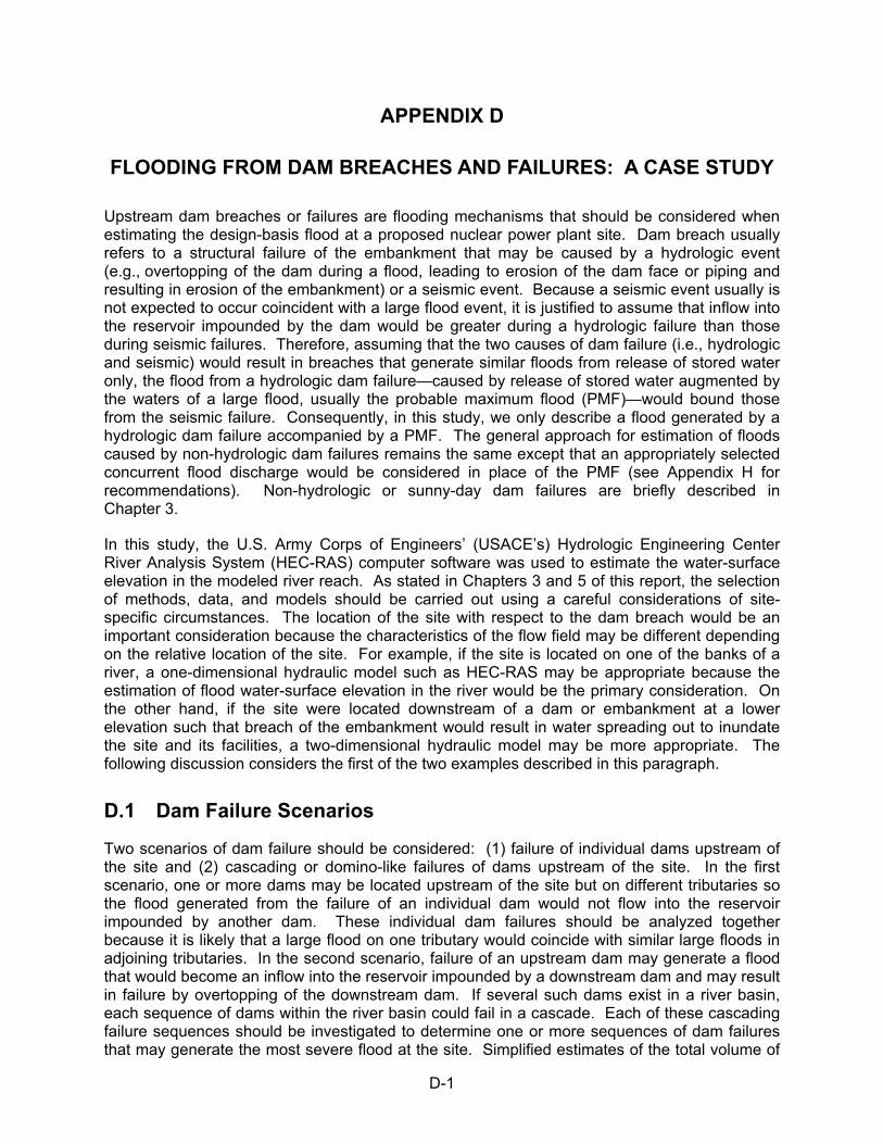
D-1
APPENDIX D
FLOODING FROM DAM BREACHES AND FAILURES: A CASE STUDY
Upstream dam breaches or failures are flooding mechanisms that should be considered when estimating the design-basis flood at a proposed nuclear power plant site. Dam breach usually refers to a structural failure of the embankment that may be caused by a hydrologic event (e.g., overtopping of the dam during a flood, leading to erosion of the dam face or piping and resulting in erosion of the embankment) or a seismic event. Because a seismic event usually is not expected to occur coincident with a large flood event, it is justified to assume that inflow into the reservoir impounded by the dam would be greater during a hydrologic failure than those during seismic failures. Therefore, assuming that the two causes of dam failure (i.e., hydrologic and seismic) would result in breaches that generate similar floods from release of stored water only, the flood from a hydrologic dam failure—caused by release of stored water augmented by the waters of a large flood, usually the probable maximum flood (PMF)—would bound those from the seismic failure. Consequently, in this study, we only describe a flood generated by a hydrologic dam failure accompanied by a PMF. The general approach for estimation of floods caused by non-hydrologic dam failures remains the same except that an appropriately selected concurrent flood discharge would be considered in place of the PMF (see Appendix H for recommendations). Non-hydrologic or sunny-day dam failures are briefly described in Chapter 3.
In this study, the U.S. Army Corps of Engineers’ (USACE’s) Hydrologic Engineering Center River Analysis System (HEC-RAS) computer software was used to estimate the water-surface elevation in the modeled river reach. As stated in Chapters 3 and 5 of this report, the selection of methods, data, and models should be carried out using a careful considerations of site-specific circumstances. The location of the site with respect to the dam breach would be an important consideration because the characteristics of the flow field may be different depending on the relative location of the site. For example, if the site is located on one of the banks of a river, a one-dimensional hydraulic model such as HEC-RAS may be appropriate because the estimation of flood water-surface elevation in the river would be the primary consideration. On the other hand, if the site were located downstream of a dam or embankment at a lower elevation such that breach of the embankment would result in water spreading out to inundate the site and its facilities, a two-dimensional hydraulic model may be more appropriate. The following discussion considers the first of the two examples described in this paragraph.
D.1 Dam Failure Scenarios
Two scenarios of dam failure should be considered: (1) failure of individual dams upstream of the site and (2) cascading or domino-like failures of dams upstream of the site. In the first scenario, one or more dams may be located upstream of the site but on different tributaries so the flood generated from the failure of an individual dam would not flow into the reservoir impounded by another dam. These individual dam failures should be analyzed together because it is likely that a large flood on one tributary would coincide with similar large floods in adjoining tributaries. In the second scenario, failure of an upstream dam may generate a flood that would become an inflow into the reservoir impounded by a downstream dam and may result in failure by overtopping of the downstream dam. If several such dams exist in a river basin, each sequence of dams within the river basin could fail in a cascade. Each of these cascading failure sequences should be investigated to determine one or more sequences of dam failures that may generate the most severe flood at the site. Simplified estimates of the total volume of
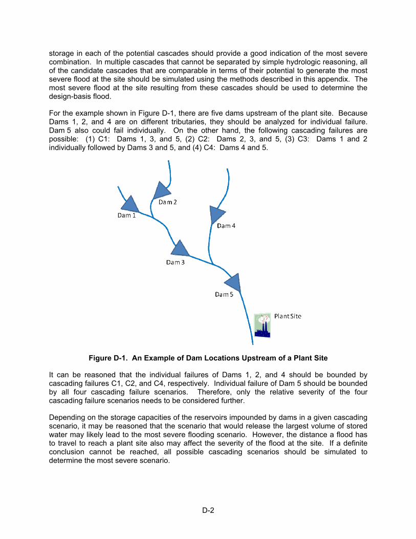
D-2
storage in each of the potential cascades should provide a good indication of the most severe combination. In multiple cascades that cannot be separated by simple hydrologic reasoning, all of the candidate cascades that are comparable in terms of their potential to generate the most severe flood at the site should be simulated using the methods described in this appendix. The most severe flood at the site resulting from these cascades should be used to determine the design-basis flood.
For the example shown in Figure D-1, there are five dams upstream of the plant site. Because Dams 1, 2, and 4 are on different tributaries, they should be analyzed for individual failure. Dam 5 also could fail individually. On the other hand, the following cascading failures are possible: (1) C1: Dams 1, 3, and 5, (2) C2: Dams 2, 3, and 5, (3) C3: Dams 1 and 2 individually followed by Dams 3 and 5, and (4) C4: Dams 4 and 5.
Figure D-1. An Example of Dam Locations Upstream of a Plant Site
It can be reasoned that the individual failures of Dams 1, 2, and 4 should be bounded by cascading failures C1, C2, and C4, respectively. Individual failure of Dam 5 should be bounded by all four cascading failure scenarios. Therefore, only the relative severity of the four cascading failure scenarios needs to be considered further.
Depending on the storage capacities of the reservoirs impounded by dams in a given cascading scenario, it may be reasoned that the scenario that would release the largest volume of stored water may likely lead to the most severe flooding scenario. However, the distance a flood has to travel to reach a plant site also may affect the severity of the flood at the site. If a definite conclusion cannot be reached, all possible cascading scenarios should be simulated to determine the most severe scenario.
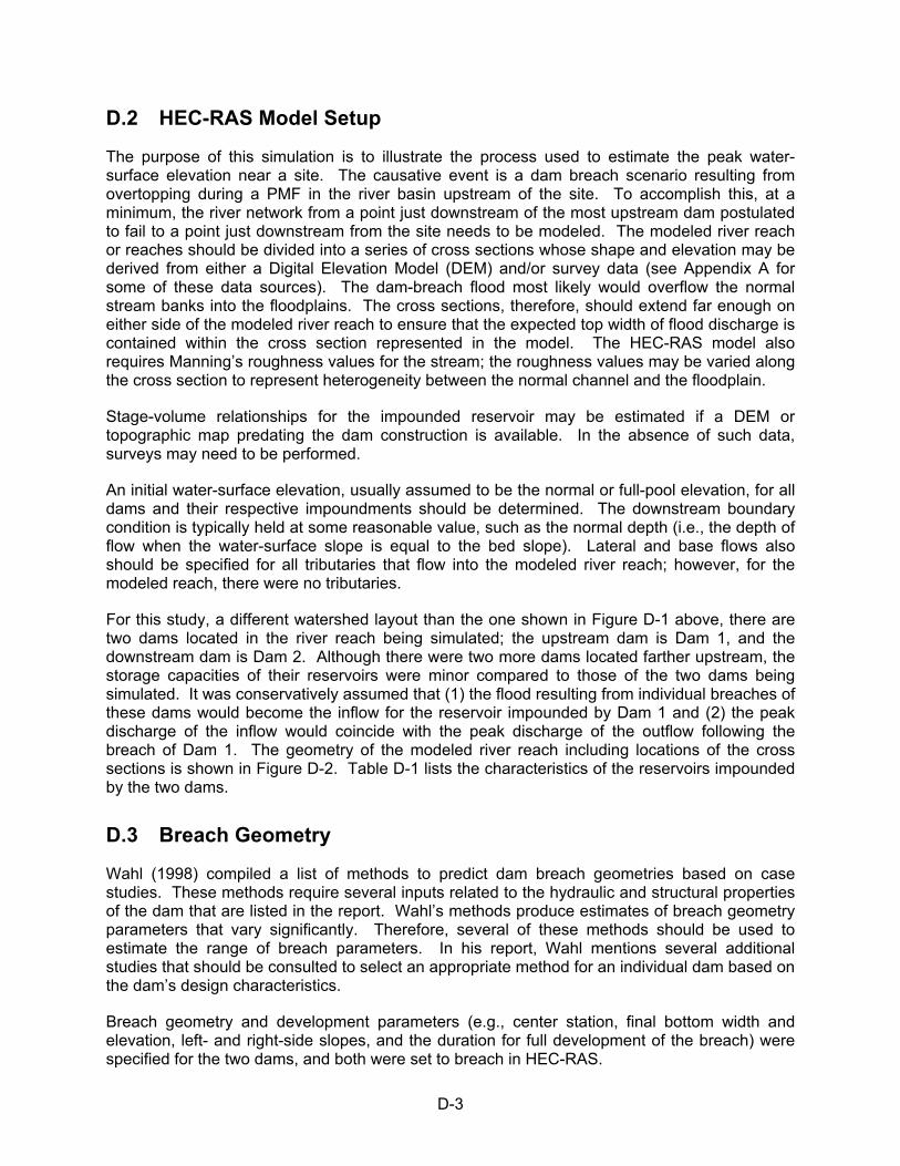
D-3
D.2 HEC-RAS Model Setup
The purpose of this simulation is to illustrate the process used to estimate the peak water-surface elevation near a site. The causative event is a dam breach scenario resulting from overtopping during a PMF in the river basin upstream of the site. To accomplish this, at a minimum, the river network from a point just downstream of the most upstream dam postulated to fail to a point just downstream from the site needs to be modeled. The modeled river reach or reaches should be divided into a series of cross sections whose shape and elevation may be derived from either a Digital Elevation Model (DEM) and/or survey data (see Appendix A for some of these data sources). The dam-breach flood most likely would overflow the normal stream banks into the floodplains. The cross sections, therefore, should extend far enough on either side of the modeled river reach to ensure that the expected top width of flood discharge is contained within the cross section represented in the model. The HEC-RAS model also requires Manning’s roughness values for the stream; the roughness values may be varied along the cross section to represent heterogeneity between the normal channel and the floodplain.
Stage-volume relationships for the impounded reservoir may be estimated if a DEM or topographic map predating the dam construction is available. In the absence of such data, surveys may need to be performed.
An initial water-surface elevation, usually assumed to be the normal or full-pool elevation, for all dams and their respective impoundments should be determined. The downstream boundary condition is typically held at some reasonable value, such as the normal depth (i.e., the depth of flow when the water-surface slope is equal to the bed slope). Lateral and base flows also should be specified for all tributaries that flow into the modeled river reach; however, for the modeled reach, there were no tributaries.
For this study, a different watershed layout than the one shown in Figure D-1 above, there are two dams located in the river reach being simulated; the upstream dam is Dam 1, and the downstream dam is Dam 2. Although there were two more dams located farther upstream, the storage capacities of their reservoirs were minor compared to those of the two dams being simulated. It was conservatively assumed that (1) the flood resulting from individual breaches of these dams would become the inflow for the reservoir impounded by Dam 1 and (2) the peak discharge of the inflow would coincide with the peak discharge of the outflow following the breach of Dam 1. The geometry of the modeled river reach including locations of the cross sections is shown in Figure D-2. Table D-1 lists the characteristics of the reservoirs impounded by the two dams.
D.3 Breach Geometry
Wahl (1998) compiled a list of methods to predict dam breach geometries based on case studies. These methods require several inputs related to the hydraulic and structural properties of the dam that are listed in the report. Wahl’s methods produce estimates of breach geometry parameters that vary significantly. Therefore, several of these methods should be used to estimate the range of breach parameters. In his report, Wahl mentions several additional studies that should be consulted to select an appropriate method for an individual dam based on the dam’s design characteristics.
Breach geometry and development parameters (e.g., center station, final bottom width and elevation, left- and right-side slopes, and the duration for full development of the breach) were specified for the two dams, and both were set to breach in HEC-RAS.
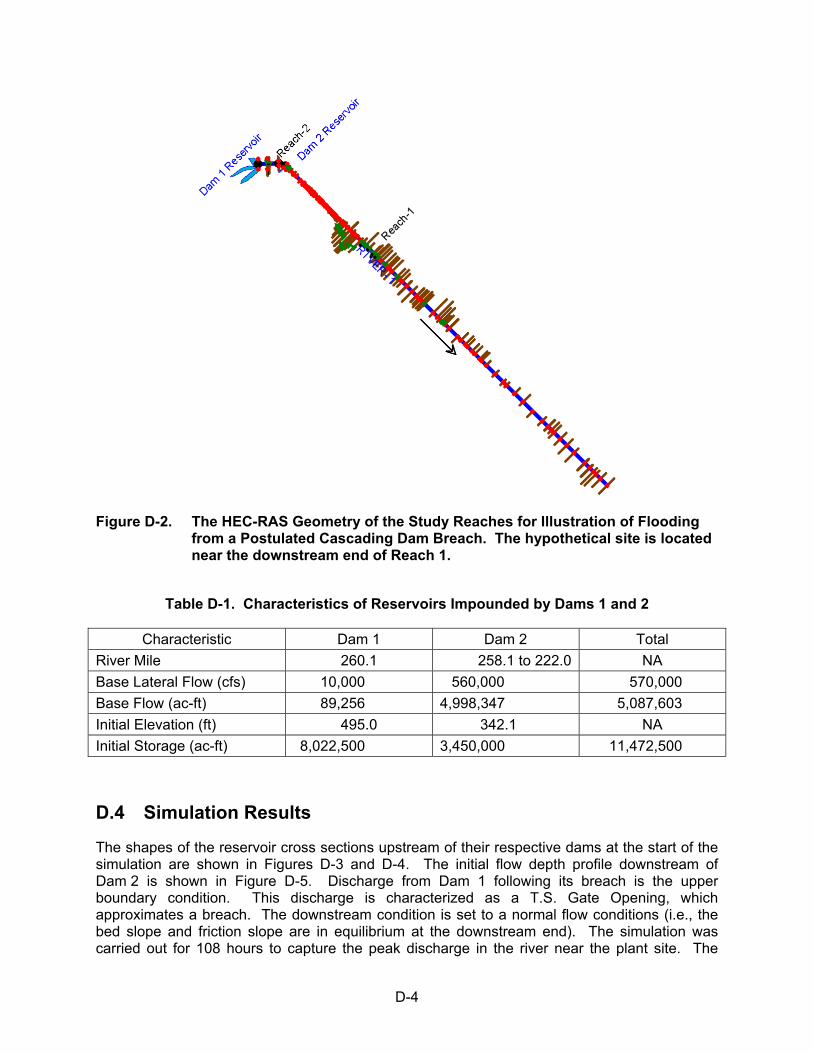
D-4
Figure D-2. The HEC-RAS Geometry of the Study Reaches for Illustration of Flooding from a Postulated Cascading Dam Breach. The hypothetical site is located near the downstream end of Reach 1.
Table D-1. Characteristics of Reservoirs Impounded by Dams 1 and 2
Characteristic Dam 1 Dam 2 Total
River Mile 260.1 258.1 to 222.0 NA
Base Lateral Flow (cfs) 10,000 560,000 570,000
Base Flow (ac-ft) 89,256 4,998,347 5,087,603
Initial Elevation (ft) 495.0 342.1 NA
Initial Storage (ac-ft) 8,022,500 3,450,000 11,472,500
D.4 Simulation Results
The shapes of the reservoir cross sections upstream of their respective dams at the start of the simulation are shown in Figures D-3 and D-4. The initial flow depth profile downstream of Dam 2 is shown in Figure D-5. Discharge from Dam 1 following its breach is the upper boundary condition. This discharge is characterized as a T.S. Gate Opening, which approximates a breach. The downstream condition is set to a normal flow conditions (i.e., the bed slope and friction slope are in equilibrium at the downstream end). The simulation was carried out for 108 hours to capture the peak discharge in the river near the plant site. The
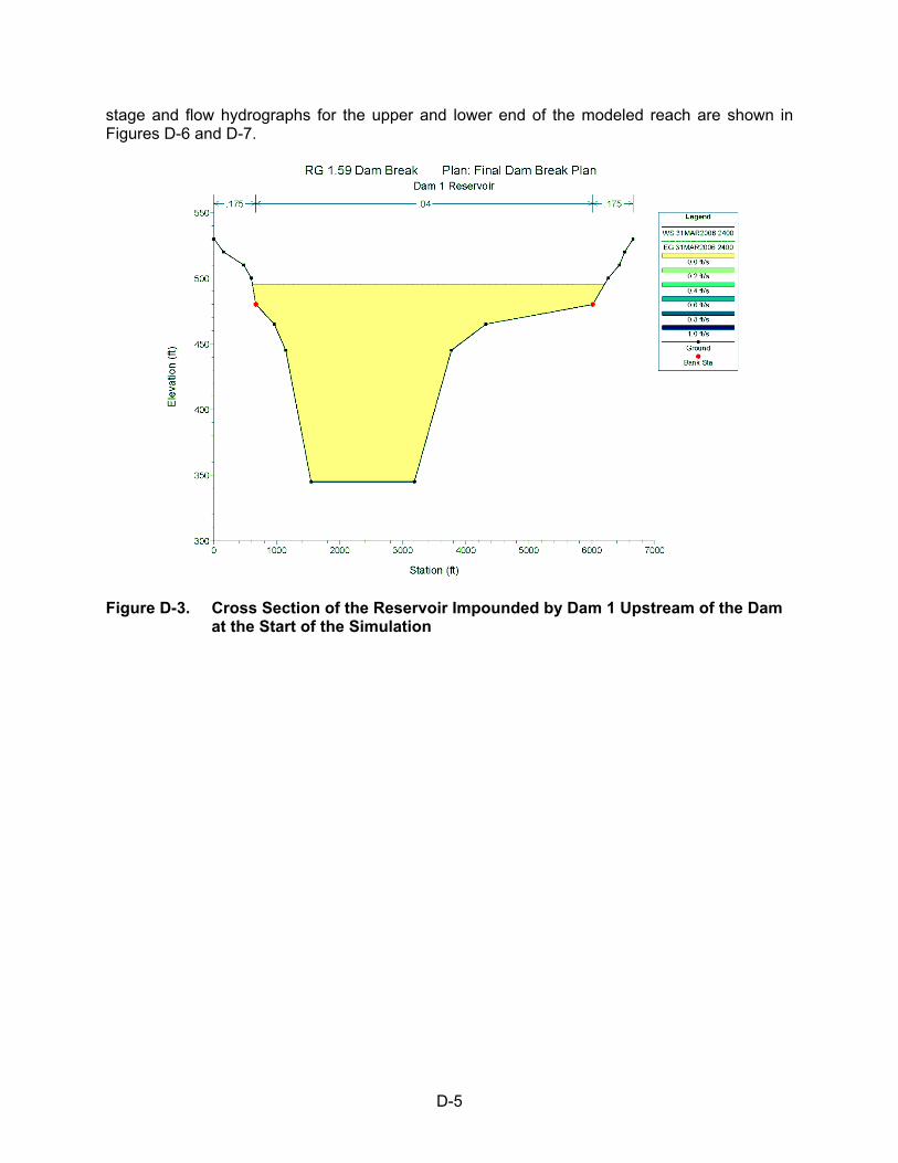
D-5
stage and flow hydrographs for the upper and lower end of the modeled reach are shown in Figures D-6 and D-7.
Figure D-3. Cross Section of the Reservoir Impounded by Dam 1 Upstream of the Dam at the Start of the Simulation
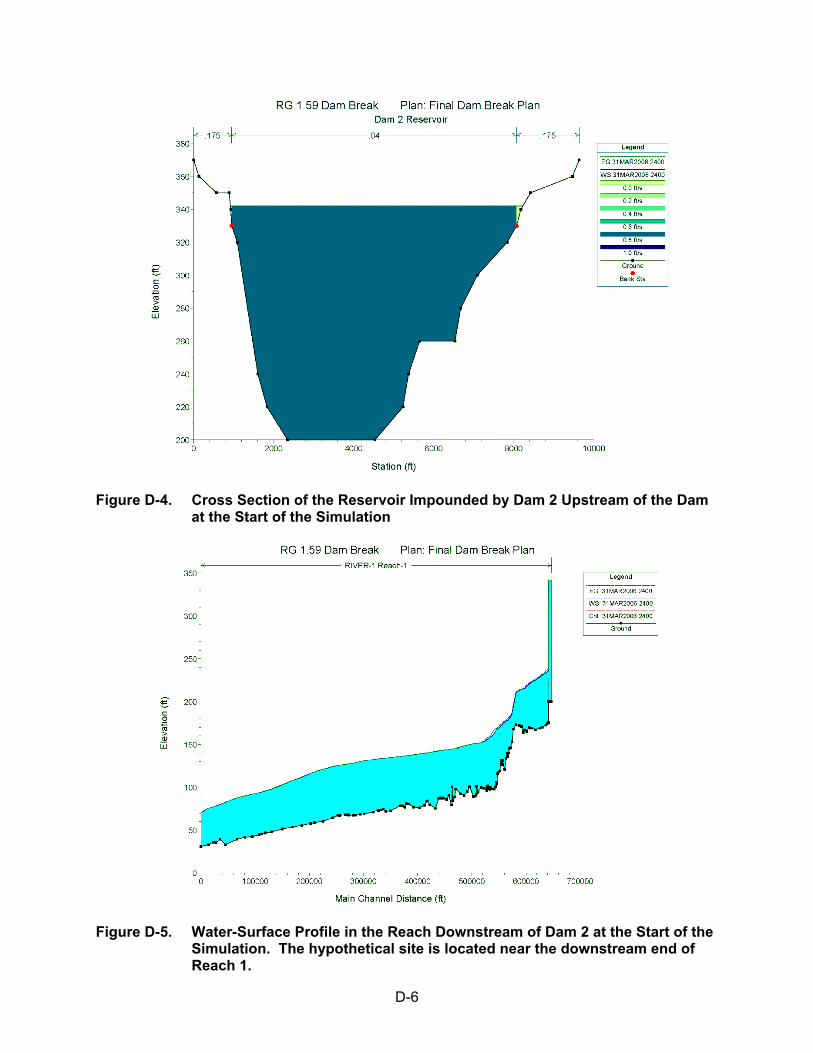
D-6
Figure D-4. Cross Section of the Reservoir Impounded by Dam 2 Upstream of the Dam at the Start of the Simulation
Figure D-5. Water-Surface Profile in the Reach Downstream of Dam 2 at the Start of the Simulation. The hypothetical site is located near the downstream end of Reach 1.
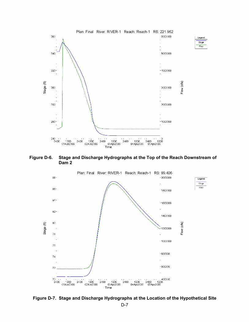
D-7
Figure D-6. Stage and Discharge Hydrographs at the Top of the Reach Downstream of Dam 2
Figure D-7. Stage and Discharge Hydrographs at the Location of the Hypothetical Site

D-8
Using the cross section at River Mile 99.406 as the location of the proposed site, the following flood information is derived from the analysis: (1) a peak discharge of 1.9 million cfs occurring 59.5 hours after the start of the simulation and (2) a corresponding still water-surface elevation of 87.3 ft.
D.5 References
Wahl T.L. 1998. Prediction of Embankment Dam Breach Parameters: A Literature Review and Needs Assessment. DSO-98-004, Dam Safety Research Report, Water Resources Research Laboratory, U.S. Department of the Interior, Bureau of Reclamation Dam Safety Office, Washington, D.C.

Appendix E
FLOODING FROM STORM SURGES: A CASE STUDY

E-1
APPENDIX E
FLOODING FROM STORM SURGES: A CASE STUDY
A storm surge is the rise in water-surface elevation along shorelines produced by the shear force of the storm winds. Areas of the Atlantic and Gulf coasts experience several hurricanes every year. In other locations, including inland locations, storm surges can be caused by severe wind storms or moving squall lines.
This appendix describes a method for estimating the probable maximum storm surge (PMSS). A PMSS is the surge that results from a combination of meteorological parameters of a probable maximum hurricane (PMH), a probable maximum wind storm, or a moving squall line and has virtually no probability of being exceeded in the region involved (NRC 2007). The PMH is a hypothetical, steady-state hurricane having a combination of values of meteorological parameters that will give the highest sustained wind speed that can probably occur at a specified coastal location (Schwerdt et al. 1979). Schwerdt et al. (1979) describe procedures to estimate the PMH wind field at any desired location along the Atlantic and Gulf Coasts of the United States.
E.1 Estimation of the PMH
The parameters that describe the PMH wind field are the difference between the peripheral pressure and the central pressure (Δp = pw - p0), the radius of maximum winds (R), the forward speed (T), and the track direction (θ). The peripheral pressure is fixed at 30.12 in. Hg or 1020 mb. In Table 3.2 of their report, Schwerdt et al. (1979) describe a step-by-step method for determining the PMH wind field using a set of calculation sheets. The procedure is semi-graphical in that a set of values from graphs and maps must be read and used in the calculation sheets. In this study, the method developed by Schwerdt et al. (1979) was implemented in spread-sheet software to facilitate the calculations.
E.2 Estimation of the PMSS from the PMH Windfield
The National Oceanic and Atmospheric Administration National Weather Service has developed a model named Sea, Lake, and Overland Surges from Hurricanes (SLOSH). Details of the SLOSH model are described by Jelesnianski et al. (1992). The model was developed as a real-time surge forecasting capability for emergency planning. It is a numerical model that approximately solves vertically averaged flow equations and yields an estimate of the elevation of the water surface. The water surface responds to changes in atmospheric pressure, wind and bottom stresses, bathymetry, and Coriolis effects. Advection terms are removed from the governing equations under the assumption that atmospheric pressure gradients and barotropic and boundary stresses are the dominant factors affecting surge elevations. The model uses a finite difference numerical scheme to estimate time-varying surge levels at discrete locations. In their publication, Jelesnianski et al. (1992) describe the computational mesh as being based on polar coordinates; however, the model has evolved and now allows parabolic and hyperbolic configurations. The meshes allow for variable spatial resolution where the mesh becomes finer in the shoreward direction and is coarser away from the shore in open waters.
A set of SLOSH simulations based on variation in hurricane parameters allows development of a maximum envelope of water (MEOW), which is defined as the maximum water-surface elevation at any given location during the simulation of storm surge from a hypothetical
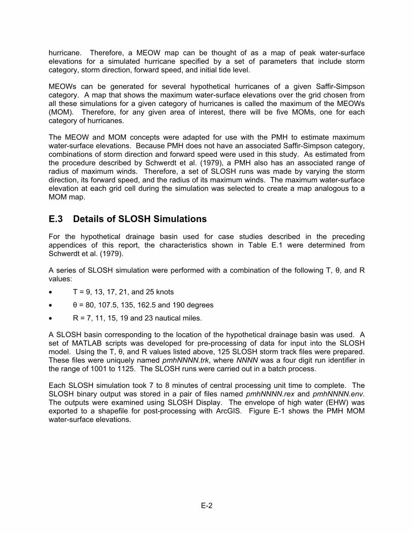
E-2
hurricane. Therefore, a MEOW map can be thought of as a map of peak water-surface elevations for a simulated hurricane specified by a set of parameters that include storm category, storm direction, forward speed, and initial tide level.
MEOWs can be generated for several hypothetical hurricanes of a given Saffir-Simpson category. A map that shows the maximum water-surface elevations over the grid chosen from all these simulations for a given category of hurricanes is called the maximum of the MEOWs (MOM). Therefore, for any given area of interest, there will be five MOMs, one for each category of hurricanes.
The MEOW and MOM concepts were adapted for use with the PMH to estimate maximum water-surface elevations. Because PMH does not have an associated Saffir-Simpson category, combinations of storm direction and forward speed were used in this study. As estimated from the procedure described by Schwerdt et al. (1979), a PMH also has an associated range of radius of maximum winds. Therefore, a set of SLOSH runs was made by varying the storm direction, its forward speed, and the radius of its maximum winds. The maximum water-surface elevation at each grid cell during the simulation was selected to create a map analogous to a MOM map.
E.3 Details of SLOSH Simulations
For the hypothetical drainage basin used for case studies described in the preceding appendices of this report, the characteristics shown in Table E.1 were determined from Schwerdt et al. (1979).
A series of SLOSH simulation were performed with a combination of the following T, θ, and R values:
• T = 9, 13, 17, 21, and 25 knots
• θ = 80, 107.5, 135, 162.5 and 190 degrees
• R = 7, 11, 15, 19 and 23 nautical miles.
A SLOSH basin corresponding to the location of the hypothetical drainage basin was used. A set of MATLAB scripts was developed for pre-processing of data for input into the SLOSH model. Using the T, θ, and R values listed above, 125 SLOSH storm track files were prepared. These files were uniquely named pmhNNNN.trk, where NNNN was a four digit run identifier in the range of 1001 to 1125. The SLOSH runs were carried out in a batch process.
Each SLOSH simulation took 7 to 8 minutes of central processing unit time to complete. The SLOSH binary output was stored in a pair of files named pmhNNNN.rex and pmhNNNN.env. The outputs were examined using SLOSH Display. The envelope of high water (EHW) was exported to a shapefile for post-processing with ArcGIS. Figure E-1 shows the PMH MOM water-surface elevations.
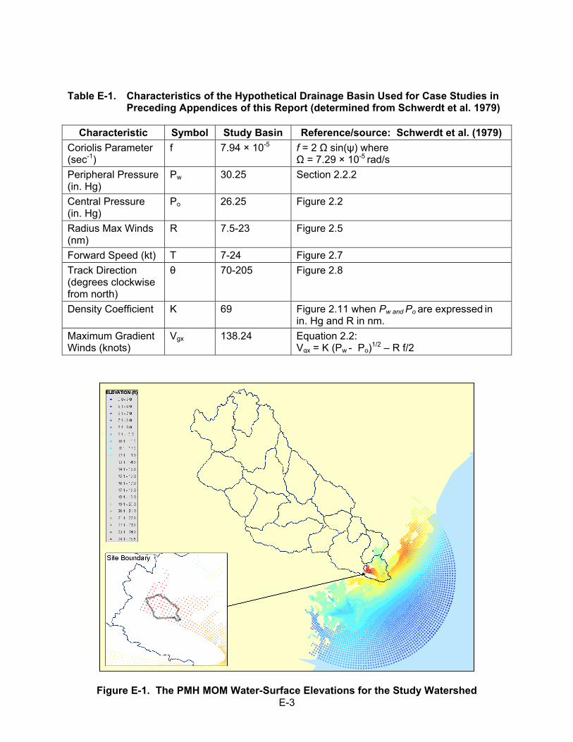
E-3
Table E-1. Characteristics of the Hypothetical Drainage Basin Used for Case Studies in Preceding Appendices of this Report (determined from Schwerdt et al. 1979)
Characteristic Symbol Study Basin Reference/source: Schwerdt et al. (1979)
Coriolis Parameter (sec-1)
f 7.94 × 10⁻⁵ f = 2 Ω sin(ψ) where Ω = 7.29 × 10⁻⁵ rad/s
Peripheral Pressure (in. Hg)
Pw 30.25 Section 2.2.2
Central Pressure (in. Hg)
Po 26.25 Figure 2.2
Radius Max Winds (nm)
R 7.5-23 Figure 2.5
Forward Speed (kt) T 7-24 Figure 2.7
Track Direction (degrees clockwise from north)
θ 70-205 Figure 2.8
Density Coefficient K 69 Figure 2.11 when Pw and Po are expressed in in. Hg and R in nm.
Maximum Gradient Winds (knots)
Vgx 138.24 Equation 2.2: Vgx = K (Pw - Po)
1/2 – R f/2
Figure E-1. The PMH MOM Water-Surface Elevations for the Study Watershed
E-4
E.4 References
Jelesnianski C.P., J. Chen, and W.A. Shaffer. 1992. SLOSH: Sea, Lake, and Overland Surges from Hurricanes. NOAA Technical Report NWS 48, National Oceanic and Atmospheric Administration National Weather Service, Silver Spring, Maryland.
Schwerdt R.W., F.P. Ho, and R.R. Watkins. 1979. Meteorological Criteria for Standard Project Hurricane and Probable Maximum Hurricane Windfields, Gulf and East Coasts of the United States. NOAA Technical Report NWS 23, National Oceanic and Atmospheric Administration, National Weather Service, Silver Spring, Maryland.
U.S. Nuclear Regulatory Commission (NRC). 2007. Standard Review Plan for the Review of Safety Analysis Reports for Nuclear Power Plants. NUREG-0800, LWR Edition, Section 2.4.5, “Probable Maximum Surge and Seiche Flooding,” Washington, D.C.

Appendix F
FLOODING FROM A SEICHE: A CASE STUDY

F-1
APPENDIX F
FLOODING FROM A SEICHE: A CASE STUDY
Generally, a seiche is defined as an oscillation of the water surface in an enclosed or semi-enclosed body of water initiated by an external cause (Wüest and Farmer 2003; Scheffner 2008). Once started, the oscillation may continue for several cycles; however, over time it gradually decays because of friction.
External initiators or forcings that can cause a seiche include barometric fluctuations, rapid changes in wind direction, storm surges, and tsunamis. An external, local seismic event also could result in “sloshing” of the water in a reservoir or basin that could lead to a seiche (USGS 2009). While the amplitude of a seiche is usually small, resonance may lead to large oscillations if the frequency of the forcing matches one of the natural periods of oscillation of the waterbody.
Because the depth of a waterbody typically is small in comparison to the wave length, seiches are generally characterized by shallow water waves. The velocity of the wave is given by the term (gh)1/2, where g is the acceleration due to gravity and h is the water depth. The natural oscillation period of an enclosed, rectangular basin can be estimated from Merian’s formula (Scheffner 2008):
T L (F-1)
In this formula, L is the length of the basin, and n is number of nodes in the standing wave. The simplest mode of oscillation of a waterbody is at the fundamental oscillation period, in which the standing wave has one node (n=1 in Merian’s formula). To estimate the oscillation period for an open rectangular basin, Scheffner (2008) modified Merian’s formula as follows:
Tn L (F-2)
In this modified formula, the fundamental period corresponds to n=0.
F.1 Estimating the Effects of Seiche in a Waterbody
An estimate of the natural oscillation period of a reservoir, lake, or bay may be obtained by applying Merian’s formula. This period may then be compared to the periods of external forcings expected in the vicinity of the waterbody. If the two periods are close in magnitude, a partial to complete resonance may occur, thus amplifying the seiche.
Merian’s formula and its modified form provide approximations only, and both formulas are based on the assumptions that the waterbody is rectangular in shape and has a uniform water depth. The natural oscillation periods of a waterbody strongly depend on its geometry and bathymetry; therefore, Merian’s formula and its modified form should be applied carefully. For more complex basin geometries and bathymetries, numerical modeling of water waves may be needed (Scheffner 2008). Rao and Schwab (1976) presented such a solution for Lake Ontario.
Scheffner (2008) describes more recent hydrodynamic models that may be applied to estimate lake and coastal seiche water levels. These models require detailed bathymetry data, and
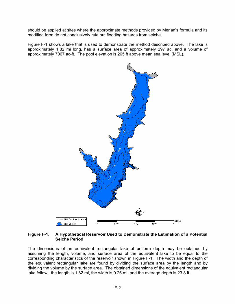
F-2
should be applied at sites where the approximate methods provided by Merian’s formula and its modified form do not conclusively rule out flooding hazards from seiche.
Figure F-1 shows a lake that is used to demonstrate the method described above. The lake is approximately 1.82 mi long, has a surface area of approximately 297 ac, and a volume of approximately 7067 ac-ft. The pool elevation is 265 ft above mean sea level (MSL).
Figure F-1. A Hypothetical Reservoir Used to Demonstrate the Estimation of a Potential Seiche Period
The dimensions of an equivalent rectangular lake of uniform depth may be obtained by assuming the length, volume, and surface area of the equivalent lake to be equal to the corresponding characteristics of the reservoir shown in Figure F-1. The width and the depth of the equivalent rectangular lake are found by dividing the surface area by the length and by dividing the volume by the surface area. The obtained dimensions of the equivalent rectangular lake follow: the length is 1.82 mi, the width is 0.26 mi, and the average depth is 23.8 ft.
F-3
Using Merian’s formula for enclosed waterbodies as stated above, the fundamental oscillation period with one node (n=1) for the equivalent rectangular lake is estimated to be approximately 11.5 min. The natural oscillation periods of expected external forcings, such as synoptic storm patterns, change in wind directions, and seismic activity expected in the vicinity of the lake, also should be determined. If the period of an external forcing is approximately equal to that of the lake, amplified seiche activity caused by resonance may occur in the lake.
More detailed investigations for seiche activity in the lake may be required if resonance is expected and if there is relatively little margin between the lake pool level and the site grade.
F.2 References
Rao D.B. and D.J. Schwab. 1976. “Two Dimensional Normal Modes in Arbitrary Enclosed Basins on a Rotating Earth: Application to Lakes Ontario and Superior.” Philosophical Transactions of the Royal Society of London, A: Mathematical and Physical Sciences 281:63-96.
Scheffner N.W. 2008. “Water Levels and Long Waves.” In: Demirbilek, Z., Coastal Engineering Manual, Part II, Coastal Hydrodynamics Chapter 5-6 , Engineer Manual 1110-2-1100, U.S. Army Corps of Engineers, Washington, D.C..
United States Geological Survey (USGS). 2009. Seismic Seiches. Available at http://earthquake.usgs.gov/learning/topics/seiche.php. Accessed May 26, 2009.
Wüest A. and D.M. Farmer. 2002. “Seiche.” McGraw-Hill Encyclopedia of Science and Technology, 9th Edition, McGraw-Hill Companies, New York.

Appendix G
FLOODING FROM ICE-INDUCED EVENTS: A CASE STUDY

G-1
APPENDIX G
FLOODING FROM ICE-INDUCED EVENTS: A CASE STUDY
Ice events can lead to two scenarios involving ice jams or dams that may result in flooding. In one scenario, ice jams or dams that form upstream of a site may collapse, thereby causing a flood that may affect a proposed nuclear power plant site. In the other scenario, ice jams or dams may form downstream of a site, causing a blockage and a backwater effect that may reach the site. Both of these scenarios may be simulated using the U.S. Army Corps of Engineers’ (USACE’s) Hydrologic Engineering Center River Analysis System (HEC-RAS) software.
G.1 Historical Ice Events
The Ice Jam Database (USACE 2009a) contains information on historical ice jams and dams, and can be queried to obtain information regarding historical ice events. For example, a query for ice events in the state of Virginia returned 22 historical events from water years 1917 to 1990 (USACE 2009b). The description field of the query results describes the events and frequently includes flood stage information. The information returned for the 1990 ice event in Virginia is shown in Figure G-1.
When assessing the potential for flooding at a proposed nuclear power plant site, information obtained from the Ice Jam Database should be used to determine the most severe historical ice-jam or ice-dam conditions, including the dam height and flood stages. These properties should be used then to postulate a hypothetical ice jam or ice dam near the proposed site.
G.2 Frazil Ice
Frazil ice forms in supercooled, turbulent water that is free of ice and snow cover (USACE 2002). Frazil ice crystals appear as elongated disks throughout the depth of the stream; these disks gradually stick together to form large ice floes and jams. For supercooling to occur, the air temperature usually must be 18ºF or lower.
Frazil ice is not related directly to flooding; however, it can be an important precursor to the formation of ice jams or dams. Therefore, the vicinity of a proposed site should be analyzed for the existence of conditions that may support the formation of frazil ice. The presence of free-flowing water, such as a stream, and low temperatures (i.e., 18ºF or lower) are two of the most important conditions that could lead to the formation of frazil ice.
Air temperature data for meteorological stations located near the site should be collected. The National Oceanic and Atmospheric Administration National Climatic Data Center (NCDC) archives daily air temperature data that can be searched and obtained interactively at the NCDC website (NCDC 2009).
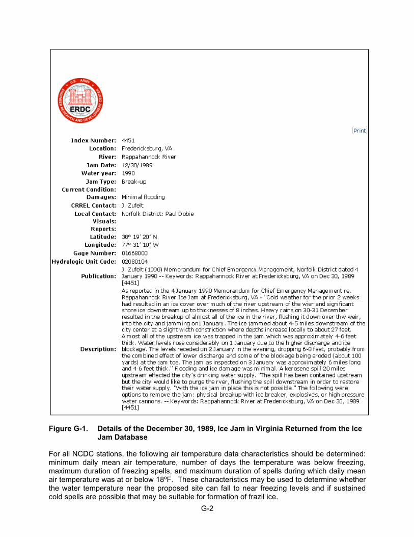
G-2
Figure G-1. Details of the December 30, 1989, Ice Jam in Virginia Returned from the Ice Jam Database
For all NCDC stations, the following air temperature data characteristics should be determined: minimum daily mean air temperature, number of days the temperature was below freezing, maximum duration of freezing spells, and maximum duration of spells during which daily mean air temperature was at or below 18ºF. These characteristics may be used to determine whether the water temperature near the proposed site can fall to near freezing levels and if sustained cold spells are possible that may be suitable for formation of frazil ice.
G-3
G.3 Bounding Analysis
Combined with the historical data from the Ice Jam Database, air temperature characteristics (see Section G.2) can be used to determine that the site does not experience conditions suitable for formation of frazil ice and ice jams or dams, specifically if there are no records of ice jams or dams in the vicinity, if the minimum air temperatures remain substantially above freezing, and if there are no periods when the air temperature is 18ºF or lower. However, if the data do not conclusively demonstrate the absence of conditions that could lead to the formation of frazil ice, the potential for ice jam and dam formation in the vicinity of a proposed site should be investigated further.
More detailed analysis for flooding from ice events would need to consider whether the most severe ice-event-induced flooding is bounded by another flooding mechanism that is relevant to the proposed site. In appreciably sized watersheds that have water-storage or flood-control impoundments, ice jams and dams may be expected to be smaller in size and, therefore, may cause floods that are smaller than those caused by breaches of impounding dams. In these situations, an analysis of the size of the flood that could be caused by breaches of impounding dams upstream of the site should be undertaken (see Appendix D). Results indicating that a flood resulting from breach of impounding dams would be larger than that from an ice event could be justification for not analyzing ice-jam or ice-dam floods in greater detail. However, if such a bounding flood is not found, the potential for ice-event-induced floods should be analyzed as described below.
G.4 Upstream Breach of an Ice Dam
The most severe historical conditions reported in the Ice Jam Database should be used to determine whether the resulting flood is bounded by floods from other upstream causal events such as the probable maximum flood and floods generated by upstream dam breaches.
If the floods from other causal events are unambiguously larger than that caused by the most severe ice jam or dam, the analysis should be documented, and no further analysis of the ice event would be needed. Otherwise, the data should be used to specify a hypothetical ice jam or dam upstream of the site. The breach of the jam or dam should be postulated conservatively so the release of impounded water would maximize the flood. The water-surface elevation in the stream reach adjacent to the proposed site should be simulated using the methods described in Appendix D.
G.5 Downstream Ice Jam and Resulting Backwater
The most severe ice jam or dam, estimated as discussed above and then placed downstream of the site on the adjoining stream, should be used to postulate conditions that may result in the most severe backwater profile adjacent to the proposed site. The most severe backwater conditions at the site would occur during an upstream flood just prior to the breach of the ice jam or dam with its height and, therefore, its ability to block the channel conveyance maximized.
The HEC-RAS software should be used to estimate the water-surface elevation in the stream reach under these conditions. The methods described in Appendix D are applicable except that the downstream ice jam or dam is not breached; however, it may be allowed to release a small discharge over and around the ice itself.
G-4
G.6 References
National Climatic Data Center. 2009. “Surface Data, Daily U.S.” Available at http://gis.ncdc.noaa.gov/website/ims-cdo/sod/viewer.htm?Box=-180:-90:180:90. Accessed May 26, 2009.
U.S. Army Corps of Engineers (USACE). 2002. Engineering and Design: Ice Engineering. Engineer Manual 1110-2-1612, U.S. Army Corps of Engineers, Washington, D.CU.S. Army Corps of Engineers (USACE). 2009a. “The Ice Jam Database.” Available at https://rsgis.crrel.usace.army.mil/icejam/. Accessed May 26, 2009.
U.S. Army Corps of Engineers (USACE). 2009b. “Historical Ice Jams in Virginia.” Available at https://rsgis.crrel.usace.army.mil/apex/f?p=273:12:1304769456164015::::P12_GETREPORT,P12_SHOWITEMS:9,0. Accessed May 26, 2009.
Appendix H
COMBINED-EFFECT FLOODS

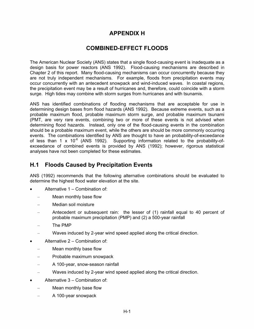
H-1
APPENDIX H
COMBINED-EFFECT FLOODS
The American Nuclear Society (ANS) states that a single flood-causing event is inadequate as a design basis for power reactors (ANS 1992). Flood-causing mechanisms are described in Chapter 2 of this report. Many flood-causing mechanisms can occur concurrently because they are not truly independent mechanisms. For example, floods from precipitation events may occur concurrently with an antecedent snowpack and wind-induced waves. In coastal regions, the precipitation event may be a result of hurricanes and, therefore, could coincide with a storm surge. High tides may combine with storm surges from hurricanes and with tsunamis.
ANS has identified combinations of flooding mechanisms that are acceptable for use in determining design bases from flood hazards (ANS 1992). Because extreme events, such as a probable maximum flood, probable maximum storm surge, and probable maximum tsunami (PMT, are very rare events, combining two or more of these events is not advised when determining flood hazards. Instead, only one of the flood-causing events in the combination should be a probable maximum event, while the others are should be more commonly occurring events. The combinations identified by ANS are thought to have an probability-of-exceedance of less than 1 x 10⁻⁶ (ANS 1992). Supporting information related to the probability-of-exceedance of combined events is provided by ANS (1992); however, rigorous statistical analyses have not been completed for these estimates.
H.1 Floods Caused by Precipitation Events
ANS (1992) recommends that the following alternative combinations should be evaluated to determine the highest flood water elevation at the site.
• Alternative 1 – Combination of:
– Mean monthly base flow
– Median soil moisture
– Antecedent or subsequent rain: the lesser of (1) rainfall equal to 40 percent of probable maximum precipitation (PMP) and (2) a 500-year rainfall
– The PMP
– Waves induced by 2-year wind speed applied along the critical direction.
• Alternative 2 – Combination of:
– Mean monthly base flow
– Probable maximum snowpack
– A 100-year, snow-season rainfall
– Waves induced by 2-year wind speed applied along the critical direction.
• Alternative 3 – Combination of:
– Mean monthly base flow
– A 100-year snowpack
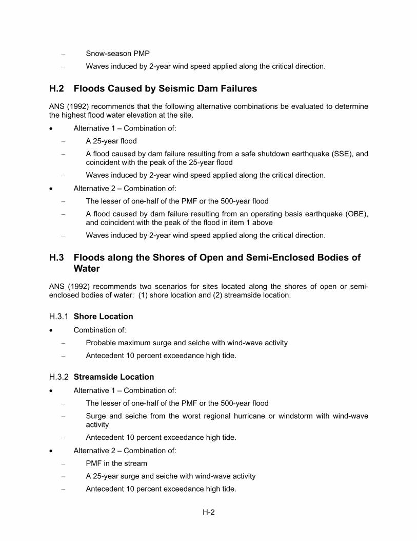
H-2
– Snow-season PMP
– Waves induced by 2-year wind speed applied along the critical direction.
H.2 Floods Caused by Seismic Dam Failures
ANS (1992) recommends that the following alternative combinations be evaluated to determine the highest flood water elevation at the site.
• Alternative 1 – Combination of:
– A 25-year flood
– A flood caused by dam failure resulting from a safe shutdown earthquake (SSE), and coincident with the peak of the 25-year flood
– Waves induced by 2-year wind speed applied along the critical direction.
• Alternative 2 – Combination of:
– The lesser of one-half of the PMF or the 500-year flood
– A flood caused by dam failure resulting from an operating basis earthquake (OBE), and coincident with the peak of the flood in item 1 above
– Waves induced by 2-year wind speed applied along the critical direction.
H.3 Floods along the Shores of Open and Semi-Enclosed Bodies of Water
ANS (1992) recommends two scenarios for sites located along the shores of open or semi-enclosed bodies of water: (1) shore location and (2) streamside location.
H.3.1 Shore Location
• Combination of:
– Probable maximum surge and seiche with wind-wave activity
– Antecedent 10 percent exceedance high tide.
H.3.2 Streamside Location
• Alternative 1 – Combination of:
– The lesser of one-half of the PMF or the 500-year flood
– Surge and seiche from the worst regional hurricane or windstorm with wind-wave activity
– Antecedent 10 percent exceedance high tide.
• Alternative 2 – Combination of:
– PMF in the stream
– A 25-year surge and seiche with wind-wave activity
– Antecedent 10 percent exceedance high tide.
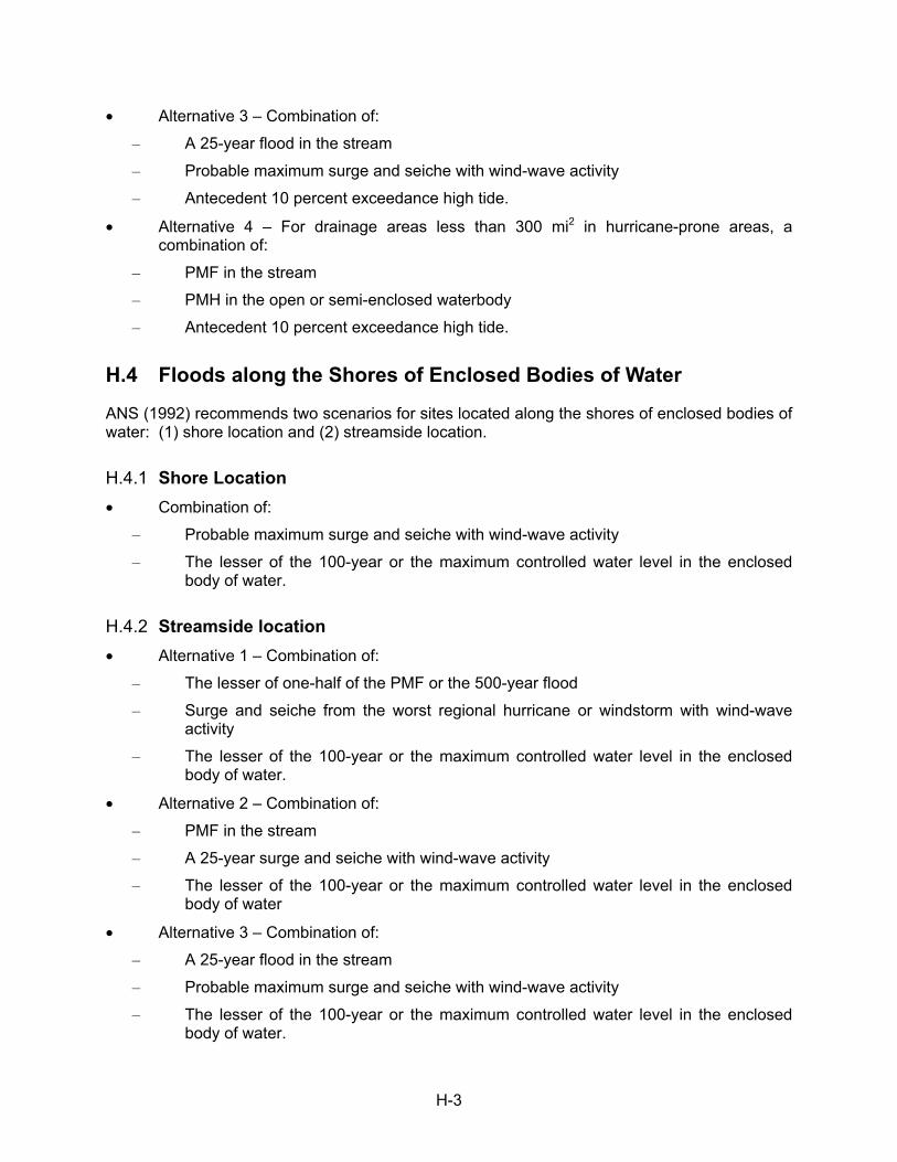
H-3
• Alternative 3 – Combination of:
– A 25-year flood in the stream
– Probable maximum surge and seiche with wind-wave activity
– Antecedent 10 percent exceedance high tide.
• Alternative 4 – For drainage areas less than 300 mi2 in hurricane-prone areas, a combination of:
– PMF in the stream
– PMH in the open or semi-enclosed waterbody
– Antecedent 10 percent exceedance high tide.
H.4 Floods along the Shores of Enclosed Bodies of Water
ANS (1992) recommends two scenarios for sites located along the shores of enclosed bodies of water: (1) shore location and (2) streamside location.
H.4.1 Shore Location
• Combination of:
– Probable maximum surge and seiche with wind-wave activity
– The lesser of the 100-year or the maximum controlled water level in the enclosed body of water.
H.4.2 Streamside location
• Alternative 1 – Combination of:
– The lesser of one-half of the PMF or the 500-year flood
– Surge and seiche from the worst regional hurricane or windstorm with wind-wave activity
– The lesser of the 100-year or the maximum controlled water level in the enclosed body of water.
• Alternative 2 – Combination of:
– PMF in the stream
– A 25-year surge and seiche with wind-wave activity
– The lesser of the 100-year or the maximum controlled water level in the enclosed body of water
• Alternative 3 – Combination of:
– A 25-year flood in the stream
– Probable maximum surge and seiche with wind-wave activity
– The lesser of the 100-year or the maximum controlled water level in the enclosed body of water.
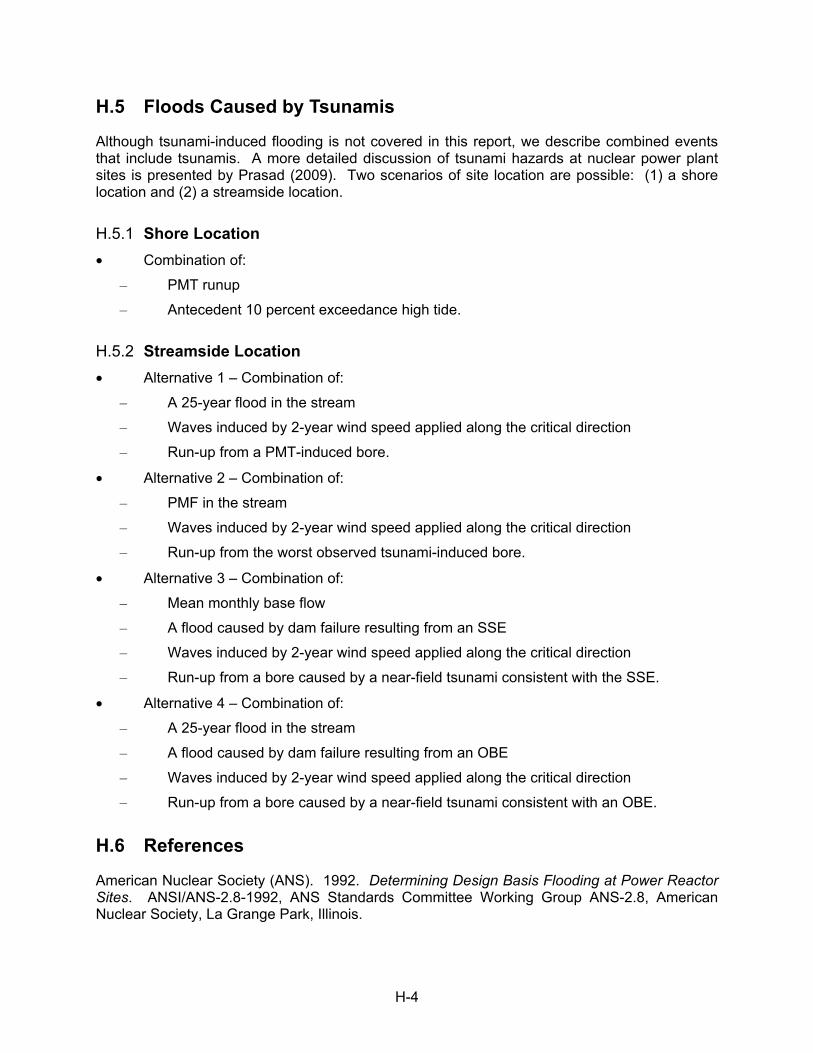
H-4
H.5 Floods Caused by Tsunamis
Although tsunami-induced flooding is not covered in this report, we describe combined events that include tsunamis. A more detailed discussion of tsunami hazards at nuclear power plant sites is presented by Prasad (2009). Two scenarios of site location are possible: (1) a shore location and (2) a streamside location.
H.5.1 Shore Location
• Combination of:
– PMT runup
– Antecedent 10 percent exceedance high tide.
H.5.2 Streamside Location
• Alternative 1 – Combination of:
– A 25-year flood in the stream
– Waves induced by 2-year wind speed applied along the critical direction
– Run-up from a PMT-induced bore.
• Alternative 2 – Combination of:
– PMF in the stream
– Waves induced by 2-year wind speed applied along the critical direction
– Run-up from the worst observed tsunami-induced bore.
• Alternative 3 – Combination of:
– Mean monthly base flow
– A flood caused by dam failure resulting from an SSE
– Waves induced by 2-year wind speed applied along the critical direction
– Run-up from a bore caused by a near-field tsunami consistent with the SSE.
• Alternative 4 – Combination of:
– A 25-year flood in the stream
– A flood caused by dam failure resulting from an OBE
– Waves induced by 2-year wind speed applied along the critical direction
– Run-up from a bore caused by a near-field tsunami consistent with an OBE.
H.6 References
American Nuclear Society (ANS). 1992. Determining Design Basis Flooding at Power Reactor Sites. ANSI/ANS-2.8-1992, ANS Standards Committee Working Group ANS-2.8, American Nuclear Society, La Grange Park, Illinois.

H-5
Prasad, R. 2009. Tsunami Hazard Assessment at Nuclear Power Plant Sites in the United States of America. NUREG/CR-6966, U.S. Nuclear Regulatory Commission, Office of New Reactors, Washington, D.C.


Appendix I
UNIT HYDROGRAPHS AND NONLINEAR HYDROLOGIC RESPONSE

I-1
APPENDIX I
UNIT HYDROGRAPHS AND NONLINEAR HYDROLOGIC RESPONSE
In precipitation-runoff analysis, the unit hydrograph (Sherman 1932) is a useful and simple to implement concept. Unit hydrographs can be estimated from observed precipitation and corresponding runoff or streamflow measurements. Unit hydrographs for ungauged drainage basins, for which observations do not exist or are insufficient, have also been estimated synthetically. The approach has, however, been controversial in terms of its technical consistency and adequacy. Some of these issues are described in this appendix.
I.1 Unit Hydrographs
A unit hydrograph is generally defined as the direct runoff hydrograph resulting from a uniform, unit depth of precipitation or rainfall excess on a drainage area. The unit hydrograph theory of runoff generation is linear, in that the direct runoff hydrograph from a rainfall excess of a given amount can simply be obtained by multiplying the unit hydrograph ordinates by that amount. It follows, then that the runoff time-base in invariant and does not depend on rainfall intensity. The main characteristics of a unit hydrograph are:
1. A runoff volume equivalent to a unit depth over the drainage area
2. A duration over which the rainfall excess occurs, and
3. A constant time-to-peak and a constant time base.
The estimation of a direct runoff hydrograph from a sequence of varying rainfall excesses is simply obtained by convolution (Chow et al. 1988):
∑ (I-1)
where Qn is the ordinate of the direct runoff hydrograph at time n (1 ≤ n ≤ N), Pm is the mth of M rainfall excesses, and U represents the unit hydrograph ordinates. The estimation of the ordinates of a unit hydrograph (U) from observed sequences of rainfall excess (P) and direct runoff hydrograph (Q) is accomplished by the reverse process, called deconvolution (Chow et al. 1988). The same set of linear equations given above is used. However, notice that there are N equations and only (N-M+1) unknowns, the ordinates of the unit hydrograph. Therefore, the system of linear equations is overdetermined. The system of linear equations can be solved to estimate the unit hydrograph with added constraints that all ordinates should be non-negative and the area under the unit hydrograph should represent unit depth of runoff from the drainage area.
The uncertainty in the estimation of the unit hydrograph arises from the uncertainty in the determination of rainfall excess, for which an estimate of rainfall loss must be made and also from the determination of the direct runoff hydrograph from the observed streamflow sequence by removing baseflow, which may vary during the runoff event and is not known with a high degree of accuracy. For these reasons, unit hydrographs estimated from observed rainfall-runoff data may exhibit oscillations, negative ordinate values, and vary in shapes for different storms. Usually an “average” unit hydrograph from several observed rainfall-runoff sequences is estimated as a compromise.
I-2
For drainage areas where little or no observed data exist, synthetic unit hydrographs have been developed (for example, Snyder 1938; Natural Resources Conservation Service, previously Soil Conservation Service (SCS) 1985; Clark 1945). These synthetic unit hydrographs relate characteristics such as time-to-peak and peak discharge to the characteristics of the drainage area (Snyder’s unit hydrographs), or are dimensionless (SCS unit hydrographs), or are based on storage effects of the drainage basin (Clark’s unit hydrographs). These approaches are well-known (Chow 1988; USACE 1994) and already implemented in standard rainfall-runoff models such as the U.S. Army Corps of Engineers’ (USACE’s) Hydrologic Engineering Center Hydrologic Modeling System (HEC-HMS) computer program.
I.2 Nonlinear Runoff Response in Drainage Basins
The rainfall-runoff process is highly nonlinear. Several sub-processes, such as interception of rainfall, throughfall, infiltration, evapotranspiration, rainfall-excess surface runoff generation, saturation-excess surface runoff generation, interflow, baseflow, and dynamic effects of open channel flow in the stream network (Dingman 2002; Chow 1959), determine the shape of the streamflow hydrograph at the outlet of a drainage area. Physically based process models, such as the Distributed Hydrology Soil-Vegetation Model (DHSVM) (Wigmosta et al. 1994, 2002) explicitly account for each of these processes to model the runoff response from a drainage area.
The unit hydrograph has been recognized to ignore the nonlinearity of the runoff generation processes (Robinson et al. 1995), particularly the invariance to rainfall intensity. Minshall (1960) estimated unit hydrographs in a small watershed in Illinois and found that they were different for different storm intensities. Pilgrim and Cordery (1993) and USACE (1991, 1994) have recommended that for simulation of the runoff response from extreme precipitation events, an adjustment of unit hydrographs derived from observed rainfall-runoff sequences is needed, particularly if the rainfall events used in the derivation of the unit hydrograph are relatively small compared to the extreme precipitation events.
The USACE (1994) cautions that the unit hydrograph used for a particular storm should be appropriate for a storm of that magnitude. The USACE (1994) recommends that unit hydrographs intended for use with large hypothetical storms should be derived from observed data of large historical events. It notes that under some conditions, it is appropriate to adjust a unit hydrograph to account for the shorter travel time of floods generated by large storm events. USACE (1991) recommended a “peaking” of 25 to 50 percent of unit hydrographs derived from smaller events in order for them to be used in the derivation of inflow design flood. Inflow design floods for dams that are capable of placing human life at risk are estimated from a probable maximum precipitation (PMP) event (USACE 1991). Pilgrim and Cordery (1993) cited studies in the United Kingdom and Australia where unit hydrograph adjustments of one-fifth increase in peak flow and a one-third reduction in time-to-peak were recommended. It is well known by kinematic wave theory that the time to equilibrium (the time to reach peak flow when the response from the whole drainage area has reached the outlet) is dependent on intensity of rainfall (Wong 1996).
Saghafian (2006) has recently demonstrated, also based on the application of kinematic wave theory, that a nonlinear transformation of the ordinates on the rising limb of a unit hydrograph derived for one rainfall intensity can be used to perfectly predict the ordinates on the rising limb of another unit hydrograph corresponding to a different rainfall intensity. These results were obtained for a constant width plane, a converging plane, and a diverging plane. However, the results of the adjustment approach for a natural drainage basin previously used by Minshall (1960) showed slight errors when several unit hydrographs estimated from different storm
I-3
events were subjected to the same transformation and compared with one of the estimated unit hydrographs (Saghafian 2006). Saghafian (2006) attributed the disagreements to possible errors in estimation of effective rainfall intensities of the relatively small storm events used by Minshall (1960).
The research for an appropriate adjustment for unit hydrographs derived from storms of intensities smaller than that of extreme design events is still ongoing. The Pacific Northwest National Laboratory is currently performing studies using DHSVM to estimate unit hydrographs from PMP events. The results of this study will be reported in the near future.
In the interim, we recommend that the unit hydrograph intended to be used for estimation of the probable maximum flood be derived from the largest historical storm events. In addition, the estimated unit hydrograph should be validated against other comparably large historical storms not used in its derivation. When the historical storms used for estimation of the unit hydrograph is significantly smaller in magnitude than the PMP, the unit hydrograph peak discharge should adjusted using the following two methods and the more conservative of the two adjusted unit hydrographs should be used further:
1. Increase the peak discharge of the unit hydrograph by one-fifth and decrease the time-to-peak by one-third.
2. Adjust the rising limb of the unit hydrograph using the approach described by Saghafian (2006) and adjust the falling limb of the unit hydrograph to preserve the runoff volume to a unit depth over the drainage area.
I.3 References
Chow V.T., “Open-Channel Hydraulics.” McGraw-Hill Book Company, New York, 680 pp., 1959.
Chow V.T., D.R. Maidment, and L.W. Mays. 1988. “Applied Hydrology.” McGraw-Hill Book Company, New York.
Clark C.O. 1945. “Storage and the unit hydrograph.” Transactions of American Society of Civil Engineers 110:1419-1488.
Dingman L.S. 2002. “Physical Hydrology.” Prentice Hall, 2nd Edition, Englewood Cliffs, New Jersey.
Minshall N.E. 1960. “Predicting storm runoff on small experimental watersheds.” Journal of Hydraulics Division, American Society of Civil Engineers 86(HY8:17–38.
Natural Resources Conservation Service (previously the U.S. Soil Conservation Service or SCS). 1985. National Engineering Handbook, Section 4, Hydrology. U.S. Department of Agriculture, Washington, D.C.
Pilgrim D.H. and I. Cordery. 1993. “Flood Runoff.” Chapter 9 in Handbook of Hydrology, D.R. Maidment (ed.), McGraw-Hill Book Company, New York.
Robinson J.S., M. Sivapalan, and J.D. Snell. 1995. “On the relative roles of hillslope processes, channel routing, and network geomorphology in the hydrologic response of natural catchments.” Water Resources Research 31(12):3089–3101.

I-4
Sherman L.K. 1932. “Streamflow from Rainfall by the Unit-graph Method.” Engineering News Record 108(1932):501–505.
Snyder F.F. 1938. “Synthetic Unit-Graphs.” , 19(1938):447-454.
U.S. Army Corps of Engineers (USACE). 1991. Inflow Design Floods for Dams and Reservoirs. Engineer Regulation 1110-8-2(FR), Washington, D.C.
U.S. Army Corps of Engineers (USACE). 1994. Flood-Runoff Analysis. Engineer Manual 1110-2-1417, Washington, D.C.
Wigmosta M.S., L. Vail, and D.P. Lettenmaier. 1994. “A distributed hydrology-vegetation model for complex terrain.” Water Resources Research 30:1665-1679.
Wigmosta M.S., B. Nijssen, P. Storck, and D.P. Lettenmaier. 2002. “The Distributed Hydrology Soil Vegetation Model,” In: Mathematical Models of Small Watershed Hydrology and Applications, V.P. Singh, D.K. Frevert (eds.), Water Resource Publications, Littleton, Colorado.
Wong T.S.W. 1996. “Influence of upstream inflow on wave celerity and time to equilibrium on an overland plane.” Hydrological Sciences 41(2):195-205.

BIBLIOGRAPHIC DATA SHEET(See instructions on the reverse)
NRC FORM 335(9-2004)NRCMD 3.7
U.S. NUCLEAR REGULATORY COMMISSION 1. REPORT NUMBER(Assigned by NRC, Add Vol., Supp., Rev.,
and Addendum Numbers, if any.)
3. DATE REPORT PUBLISHED
MONTH YEAR
4. FIN OR GRANT NUMBER
2. TITLE AND SUBTITLE
5. AUTHOR(S) 6. TYPE OF REPORT
7. PERIOD COVERED (Inclusive Dates)
8. PERFORMING ORGANIZATION - NAME AND ADDRESS (If NRC, provide Division, Office or Region, U.S. Nuclear Regulatory Commission, and mailing address; if contractor,
9. SPONSORING ORGANIZATION - NAME AND ADDRESS (If NRC, type "Same as above"; if contractor, provide NRC Division, Office or Region, U.S. Nuclear Regulatory Commission,
provide name and mailing address.)
and mailing address.)
10. SUPPLEMENTARY NOTES
11. ABSTRACT (200 words or less)
12. KEY WORDS/DESCRIPTORS (List words or phrases that will assist researchers in locating the report.)
14. SECURITY CLASSIFICATION
13. AVAILABILITY STATEMENT
unlimited
(This Page)
unclassified(This Report)
unclassified15. NUMBER OF PAGES
16. PRICE
NRC FORM 335 (9-2004) PRINTED ON RECYCLED PAPER
NUREG/CR-7046
PNNL-20091
Design-basis Flood Estimation for Site Characterization at Nuclear Power Plants in theUnited States of America November 2011
N6575
Rajiv Prasad, Lyle F. Hibler, Andre M. Coleman, and Duane L. Ward, Pacific NorthwestNational Laboratory
Technical
Not Applicable
Pacific Northwest National LaboratoryP.O. Box 999Richland, WA 99352
Office of Nuclear Regulatory ResearchDivision of Fuel, Engineering, and Radiological ResearchU.S. Nuclear Regulatory CommissionWashington, DC 20555
John Randall, NRC Project Manager; Thomas Nicholson, NRC Technical Monitor
The purpose of this document is to describe approaches and methods for estimation of the design-basis flood at nuclear powerplant sites. We define the design-basis flood and list the relevant U.S. Nuclear Regulatory Commission’s (NRC) regulations.The concepts of hierarchical hazard assessment (HHA) and alternative conceptual models are introduced. The individualflood-causing mechanisms and their effects are described. A description of the HHA method as applied to several of theseflooding mechanisms is provided. A brief discussion of combined events is also included. Two analytical approaches, thedeterministic and the probabilistic, used in standard engineering practice for estimation of design-basis floods are described.The NRC’s quality assurance criteria for simulation models are described. A description of criteria used in selection ofsimulation models is included. Uncertainty in input data and model parameters is discussed. A brief discussion of verification ofmodel-derived estimates is also included. We present an outline of the components of a formal Probabilistic Flood HazardAssessment approach. We briefly describe the findings of the fourth assessment report on climate change prepared by theIntergovernmental Panel on Climate Change. We briefly describe incorporation of the effects of climate change in estimation ofthe design-basis floods. We provide a few specific recommendations for further research. Incorporation of more recentsite-specific datasets to demonstrate the validity of estimated design-basis floods would provide additional assurance regardingavailable margins. Development of a comprehensive probabilistic flood hazard assessment methodology that leverages existingtechniques and accounts for uncertainty in model inputs and parameters can provide an extremely useful tool for risk-informeddesign-basis flood estimation at nuclear power plant sites.
design-basis flood, hierarchical hazard assessment, flood-causing mechanisms, alternativeconceptual models, probable maximum flood, probable maximum storm surge, paleo-flood, localintense precipitation, dam failure, dam breach


UN
ITE
D S
TAT
ES
N
UC
LE
AR
RE
GU
LA
TO
RY
CO
MM
ISS
ION
WA
SH
ING
TO
N, D
C 20555-0001
--------------------O
FF
ICIA
L BU
SIN
ES
S

NU
REG
/CR
-7046
Design-B
asis Flood Estimation for Site C
haracterization at N
uclear Power Plants in the U
nited States of Am
erica N
ovember 2011