Design, Construction and Control of a Quadrotor Helicopter ... · Design, Construction and Control of a Quadrotor Helicopter Using a New Multirate Technique Camilo Ossa-G omez´ A

Design, Construction and Control of a Quadrotor

Helicopter Using a New Multirate Technique

Camilo Ossa-Gomez

A Thesis

in

The Department

of

Electrical and Computer Engineering

Presented in Partial Fulfillment of the Requirements

for the Degree of Master of Applied Science (Electrical and Computer Engineering) at

Concordia University

Montreal, Quebec, Canada

June 2012

c© Camilo Ossa-Gomez, 2012

CONCORDIA UNIVERSITY

School of Graduate Studies

This is to certify that the thesis proposal prepared

By: Camilo Ossa-Gomez

Entitled: Design, Construction and Control of a Quadrotor Helicopter Using a

New Multirate Technique

and submitted in partial fulfilment of the requirements for the degree of

Master of Applied Science (Electrical and Computer Engineering)

complies with the regulations of this University and meets the accepted standards with

respect to originality and quality.

Signed by the final examining committee:

Dr. L. A. Lopes, Chair

Dr. Dr. R. Dssouli, Examiner, External

Dr. A. Aghdam, Examiner

Dr. L. Rodrigues, Supervisor

Approved by

Dr. W. E. Lynch, Chair

Department of Electrical and Computer Engineering

Dr. Robin A. L. Drew

Dean, Faculty of Engineering and Computer Science

ABSTRACT

Design, Construction and Control of a Quadrotor Helicopter Using a New Multirate

Technique

Camilo Ossa-Gomez

This thesis describes the design, development, analysis and control of an autonomous

Quadrotor Uninhabited Aerial Vehicle (UAV) that is controlled using a novel approach for

multirate sampled-data systems. This technique uses three feedback loops: one loop for

attitude, another for velocity and a third loop for position, yielding a piece-wise affine sys-

tem. Appropriate control actions are also computed at different rates. It is shown that this

technique improve the system’s stability under sampling rates that are significantly lower

than the ones required with more classical approaches. The control strategy, that uses sen-

sor data that is sampled at different rates in different nodes of a network, is also applied

to a ground wheeled vehicle. Simulations and experiments show very smooth tracking of

set-points and trajectories at a very low sampling frequency, which is the main advantage

of the new technique.

iii

“If we knew what it was we were doing,

it would not be called research, would it?”

— Albert Einstein

“There are trivial truths and there are great truths.

The opposite of a trivial truth is plainly false.

The opposite of a great truth is also true.”

— Niels Bohr

iv

ACKNOWLEDGEMENTS

I would like to thank my supervisor, Dr. Luis Rodrigues. I could not have accom-

plished my academic goals without your guidance and support. Being a member of the

HYCONS Laboratory was a very rewarding experience. I am also very grateful to the

examining committee, Dr. Luiz Lopes, Dr. Rachida Dssouli and Dr. Amir Aghdam. Their

valuable comments led to important improvements in this thesis.

I would also like to thank my colleagues for their help and friendship. They are:

Miad Moarref, Amin Zavieh, Sina Kaynama, Gavin Kenneally, Hadi Karimi, Azita Malek,

Qasim Bhojani, Mehdi Abedinpour, Behnam Gholitabar, Behzad Samadi, Mohsen Za-

mani, Jamila Raouf, Gareth Dicker, Amer Alhalabi, Rami Jaber, Anas Salah and Andrew

Bichouti. Moreover, I would like to thank all my friends and specially Luisa for their

support and all those great moments that we spent together.

Last but not least, I would like to express my immense gratitude to my father, my

mother and my brother for their love and support during my graduate studies.

v

TABLE OF CONTENTS

List of Figures ix

List of Tables xi

1 Introduction 1

1.1 Motivation . . . . . . . . . . . . . . . . . . . . . . . . . . . . . . . . . . 1

1.2 Literature Survey . . . . . . . . . . . . . . . . . . . . . . . . . . . . . . 4

1.2.1 Quadrotor helicopters . . . . . . . . . . . . . . . . . . . . . . . . 4

1.2.2 Fly by wireless . . . . . . . . . . . . . . . . . . . . . . . . . . . 5

1.2.3 Multirate control . . . . . . . . . . . . . . . . . . . . . . . . . . 6

1.3 Objectives and contributions . . . . . . . . . . . . . . . . . . . . . . . . 7

1.4 Structure of the Thesis . . . . . . . . . . . . . . . . . . . . . . . . . . . 8

2 Quadrotor Design, Construction and Modeling 10

2.1 General requirements, specifications and design considerations . . . . . . 10

2.2 Wireless communications . . . . . . . . . . . . . . . . . . . . . . . . . . 11

2.3 Electronics and sensors . . . . . . . . . . . . . . . . . . . . . . . . . . . 12

2.3.1 Processing Unit . . . . . . . . . . . . . . . . . . . . . . . . . . . 13

2.3.2 Inertial Measurement Unit (IMU) . . . . . . . . . . . . . . . . . 15

2.3.3 Electronic Speed Controllers (ESC) . . . . . . . . . . . . . . . . 16

2.3.4 Magnetometer . . . . . . . . . . . . . . . . . . . . . . . . . . . 16

2.3.5 Ultrasonic range finder . . . . . . . . . . . . . . . . . . . . . . . 17

2.3.6 Machine Vision System . . . . . . . . . . . . . . . . . . . . . . 17

2.4 Mechanics . . . . . . . . . . . . . . . . . . . . . . . . . . . . . . . . . . 19

2.4.1 Mechanical structure . . . . . . . . . . . . . . . . . . . . . . . . 19

2.4.2 Motors and propellers . . . . . . . . . . . . . . . . . . . . . . . 20

vi

2.5 Modeling . . . . . . . . . . . . . . . . . . . . . . . . . . . . . . . . . . 21

3 Kinematics control 24

3.1 General concepts and notation . . . . . . . . . . . . . . . . . . . . . . . 25

3.2 Quadrotor Helicopter . . . . . . . . . . . . . . . . . . . . . . . . . . . . 27

3.2.1 Velocity control . . . . . . . . . . . . . . . . . . . . . . . . . . . 30

3.2.2 Position control . . . . . . . . . . . . . . . . . . . . . . . . . . . 31

3.2.3 Simulation results . . . . . . . . . . . . . . . . . . . . . . . . . 33

3.3 Land rover . . . . . . . . . . . . . . . . . . . . . . . . . . . . . . . . . . 34




3.4 Stability analysis and velocity of convergence . . . . . . . . . . . . . . . 41

4 Dynamics Control and Experimental Results 46

4.1 Quadrotor Helicopter . . . . . . . . . . . . . . . . . . . . . . . . . . . . 46

4.1.1 Attidude control . . . . . . . . . . . . . . . . . . . . . . . . . . 47




4.1.5 Experimental results . . . . . . . . . . . . . . . . . . . . . . . . 56

4.2 Unicycle . . . . . . . . . . . . . . . . . . . . . . . . . . . . . . . . . . . 57

4.2.1 Heading angle tracking control . . . . . . . . . . . . . . . . . . . 58




4.2.5 Experimental results . . . . . . . . . . . . . . . . . . . . . . . . 62

4.2.6 Singular perturbations analysis . . . . . . . . . . . . . . . . . . . 66

vii

5 Conclusions 68

viii

LIST OF FIGURES

1.1 De Bothezat quadrotor, 1922 [4] . . . . . . . . . . . . . . . . . . . . . . 4

1.2 Commercial modern Quadrotor UAVs from ETH Zurich [17] . . . . . . . 5

1.3 Fly-by-wireless aircraft flight control system [28] . . . . . . . . . . . . . 6

2.1 Proposed wireless control approach for the quadrotor . . . . . . . . . . . 12

2.2 XBee Modules [46] . . . . . . . . . . . . . . . . . . . . . . . . . . . . . 13

2.3 Electronics schematic . . . . . . . . . . . . . . . . . . . . . . . . . . . . 14

2.4 Arduino Mega Board [49] . . . . . . . . . . . . . . . . . . . . . . . . . 15

2.5 MicroStrain 3DM-GX1 IMU [50] . . . . . . . . . . . . . . . . . . . . . 16

2.6 Maxbotix LV-MaxSonar-EZ4 [52] . . . . . . . . . . . . . . . . . . . . . 17

2.7 Machine Vision system camera . . . . . . . . . . . . . . . . . . . . . . . 18

2.8 Render from the CAD model of the quadrotor. . . . . . . . . . . . . . . . 19

2.9 Picture of the HYCONS quadrotor . . . . . . . . . . . . . . . . . . . . . 20

3.1 Multirate control loops . . . . . . . . . . . . . . . . . . . . . . . . . . . 25

3.2 Longitudinal model of the quadrotor. . . . . . . . . . . . . . . . . . . . . 28

3.3 Quadrotor’s control loops . . . . . . . . . . . . . . . . . . . . . . . . . . 29

3.4 Quadrotor’s velocity tracking . . . . . . . . . . . . . . . . . . . . . . . . 32

3.5 Simulation plots of the quadrotor’s kinematic control . . . . . . . . . . . 35

3.6 Illustration of a unicycle . . . . . . . . . . . . . . . . . . . . . . . . . . 36

3.7 Unicycle’s control loops. . . . . . . . . . . . . . . . . . . . . . . . . . . 37

3.8 Kinematic control simulation of the unicycle . . . . . . . . . . . . . . . . 41

3.9 Phase plane plot of the unicycle’s kinematic control . . . . . . . . . . . . 42

4.1 Quadrotor’s control loops . . . . . . . . . . . . . . . . . . . . . . . . . . 47

4.2 Attitude-tracking controller simulation . . . . . . . . . . . . . . . . . . . 50

ix

4.3 Dynamics control simulation of the HYCONS quadrotor model . . . . . . 55

4.4 Experimental results obtained with the HYCONS Helicopter . . . . . . . 57

4.5 Unicycle dynamics simulation results . . . . . . . . . . . . . . . . . . . 62

4.6 Phase plane plot of the unicycle’s dynamics control . . . . . . . . . . . . 63

4.7 Experimental results obtained with the HYCONS Rover . . . . . . . . . 64

4.8 Further experimental results obtained with the HYCONS Rover . . . . . 65

x

LIST OF TABLES

2.1 HYCONS Quadrotor main components . . . . . . . . . . . . . . . . . . 18

2.2 E-flite 370 Brushless Outrunner Motor characteristics. Information ex-

tracted from [55] . . . . . . . . . . . . . . . . . . . . . . . . . . . . . . 21

3.1 Parameters for the quadrotor’s kinematic control simulation . . . . . . . . 33

3.2 Simulation parameters for the unicyle’s kinematic control . . . . . . . . . 40

4.1 Simulation parameters for the attitude-tracking controller simulation . . . 49

4.2 Parameters for the quadrotor’s dynamics control simulation . . . . . . . . 56

4.3 Simulation parameters for the unicyle’s dynamics control . . . . . . . . . 61

4.4 HYCONS Rover experiment’s parameters . . . . . . . . . . . . . . . . . 63

xi

Chapter 1

Introduction

1.1 Motivation

Uninhabited Vehicles (UVs) have motivated a significant amount of research in diverse

fields during the last decades. UVs are no longer a topic of interest only for scientists

and engineers, but also for the general public. From self-driving cars to autonomous

home cleaning devices and radio-controlled mini air vehicles, UVs are getting closer to

everyday life. Moreover, Uninhabited Air Vehicles (UAV), have attracted great attention,

partly because of the many potential applications they have, such as mapping, surveillance,

fire fighting, exploration, and support of rescue operations, to name a few. In particular,

quadrotor helicopters are getting special attention during the last two decades. In addi-

tion to the obvious advantages of using UAVs in missions where hazardous conditions for

human pilots are involved, a quadrotor offers some edges over fixed-wing aircrafts such

as the ability of Vertical Take-off and Landing (VTOL) and hovering. Furthermore, its

maneuverability and small size makes it suitable for indoor flight.

One of the main challenges of controlling a quadrotor comes from the fact that they

are inherently unstable and some of their physical variables have a relatively fast dynamic

1

behavior. These characteristics require a fast sampling rate to maintain the system’s stabil-

ity. If there are wireless communications involved in the control tasks, the used protocol

must be able to provide a transfer rate fast enough that will not add significant delays that

could negatively affect the performance of the aircraft.

Fly-by-wireless (FBW) is a technology trend driven mainly by the aerospace indus-

try, aiming at improving the efficiency and reliability of aircrafts while reducing opera-

tional costs from maintenance by decreasing the amount and complexity of its wiring. An

evolution of fly-by-wire technology, FBW not only keeps the assets of its predecessor,

but also adds advantages such as scalability, flexibility, less wiring weight and reduced

chances of hardware failure at connectors and wires, amongst others [1].

Multirate control, on the other hand, is an intuitively efficient way to control systems

in which several variables with different dynamical time-constants are interacting with

each other. It is a known fact that fast variables require faster sampling rates than the slower

ones. In addition, when several sensors are used in a system they usually have different

update rates. In modern control applications, including vehicles, most sensors are digitally

interfaced with the control processing unit at given sampling rate. That rate depends on a

number of factors that are specific to each sensor; they usually have embedded processing

units dedicated to perform specific tasks that are needed to obtain reliable measurements

of the variables. Reading the analog measurements of the sensors, filtering the signals

and managing the communication with the main processor are some of the typical tasks

of these embedded processors. Therefore, each sensor has a different sampling frequency.

Multirate control takes advantage of this fact, allowing different rates for different sets of

variables in the control loop.

A controller that is able to handle multiple rates has two main advantages:

1. It can manage a system in which different sensors provide measurements at different

fixed rates

2. It allows to optimize the sampling frequencies and computational load for the case

2

of sensors that can be polled.

A controller that is able to handle multiple rates has two main advantages: First, it

can manage a system in which different sensors provide measurements at different fixed

rates; second, it allows to optimize the sampling frequencies and computational load for

when sensors that can be polled are used.

In some applications where a Global Positioning System is not available, such as the

Mars Exploration Rovers, position estimations are based on Visual Target Tracking (VTT)

and Visual Odometry (Visodom). The position updates using these systems can take up to

1 minute using VTT, and 2-3 minutes using Visodom [2]. When such low sampling fre-

quencies are the only source of information for position in a navigation system, multirate

control techniques that are robust under these conditions are required.

When considered separately, the topics mentioned in the previous paragraphs have

been active research fields during the last decades. However, to the best of our knowledge

there are no results combining these three topics in the open literature. The goal of this

thesis is threefold. The first component is the development of a quadrotor helicopter to be

used as a test platform to implement the control strategies and algorithms. The second is

to design controllers using FBW technology in the test platform. The network limitations

and constraints will be analyzed to predict how they influence the system’s stability and

performance, and the output of that process will be considered during the control design to

develop algorithms that are compliant with these possible limitations. Finally, a multirate

controller will be designed, analyzed and implemented, inspired by the nature of the dif-

ferent dynamical behavior of the variables involved during the operation of the quadrotor.

Additionally, it will be shown that the developed multirate strategy is suitable for a wide

variety of vehicles, and this strategy will also be implemented on an autonomous land

rover.

3

1.2 Literature Survey

1.2.1 Quadrotor helicopters

The first quadrotor helicopter took off in 1922. It was built by George de Bothezat for the

United States Army Air Service, and although the prototype was successful, the program

was canceled one year later, allegedly because of its mechanical complexity, reliability

problems, and because it was unresponsive and underpowered [See Figure 1.1]. Although

other projects further explored four-propeller helicopters, there is few information in the

open literature [3].

Figure 1.1: De Bothezat quadrotor, 1922 [4]

The four-propeller architecture started to gain relevance during the 1990s and be-

came an active research field since the beginning of the last decade. Projects such as the

HoverBot [5], and the Mesicopter [6] explored the possibility of an electrically powered

quadrotor. Atug et. al. [7] were the first ones to use the term quadrotor in a publication in

the open academic literature. They modeled the quadrotor using Newton-Euler’s laws and

attempted its stabilization and tracking using visual feedback as the main sensor. Later,

Moktari et. al. [8] designed a state parameter control based on Euler angles and state po-

sition observer for a nonlinear dynamic model. Several different strategies such as sliding

mode observers [9], neural networks [10] and PD2 feedback based on the compensation

of the Coriolis and gyroscopic torques [11], to name a few, were also implemented during

4

the last decade.

More recent research on quadrotor control has also addressed several approaches,

including model predictive control [12], dynamic inversion [13], nested saturations, back-

stepping and sliding modes [14] and H∞ control [15]. Multirate control has been addressed

in [16] using lifting operators, where only attitude and altitude were considered, reducing

the problem to a fully-actuated system.

Figure 1.2: Commercial modern Quadrotor UAVs from ETH Zurich [17]

Mellinger et. al. [18] from the GRASP Laboratory at University of Pennsylvania and

Hoffmann, et. al. [19] from Stanford and Waterloo Universities, have focused on trajectory

generation and control for aggressive maneuvers with quadrotors. D’Andrea et. al. have

conducted research in a number of different fields and applications for quadrotors such

as ball juggling [20], trajectory generation [21], acrobatic maneuvers [22], choreography

with several helicopters [23] and control of an inverted pendulum mounted on a quadrotor

[24]. Figure 1.2 shows a commercial modern quadrotor used in research at the GRASP

Laboratory.

1.2.2 Fly by wireless

The first time that the term ”Fly-by-wireless” was used in the open academic literature

was in 2001 in a paper by P. Wiberg and U. Bilstrup [25]. They discussed the possibility

5

of implementing a FBW channel in an aircraft and discussed the order of magnitude of the

bit error probability. Carvalhal et. al. [26], [27] were the first ones to implement FBW

technology in a UAV fixed-wing aircraft using Bluetooth protocol. Belapurkar et. al. [28]

and H. Liu [29] proposed Wireless Sensor Networks (WSN) for aircraft control, health

management systems and fault diagnosis. Figure 1.3 illustrates a FBW aircraft control

system scheme implemented on a military aircraft [28]. Taajwar et. al. [30] propose

the use of a CDMA and single-wire-line technology as a potential solution for Fly-by-

wireless/less-wire. Elgezabal et. al. [32] did an extensive state of the art exploration

of wireless data transmission to provide technological foundation for future intra-aircraft

wireless applications. S. Chilakala [33] and D. Hope [34] implemented IEEE 802.11 and

ZigBee protocols in a UAV. The former also studies intra-aircraft wireless propagation

phenomena such as resonant cavity, and reverberation chamber.

Figure 1.3: Fly-by-wireless aircraft flight control system [28]

1.2.3 Multirate control

Research on multirate control started in the 1950’s. D. Kranc [35], started the analysis of

sampled-data systems with different sampling rates using Z-transform methods. B Fried-

land [36] developed the concept of lifting operators, setting the general framework for

multirate control systems analysis. J. Johnson et. al. [37] further continued the analysis of

6

multirate digital control systems by studying the error induced by the quantization of sig-

nals. D. Flowers et. al. [38] proposed a method to simplify the characteristic equations of

multirate control systems and proposed the first design techniques specifically conceived

for this class of systems. Boykin et. al. [40] proposed the analysis of multirate control

systems using vector operators to obtain modified Z-transforms.

Recent results on multirate control systems include techniques to eliminate ripple

[41], applications to networked Internet-based control systems [43] and tracking control

based on multirate feedforward control with generalizations of sampling periods [42]. Re-

cent applications include visual servoing of manipulators [44] and radial control tracking

in high-speed DVD players [45].

1.3 Objectives and contributions

The main objectives and contributions of this thesis are twofold. In terms of theory, the

main novelty is the proposed multirate control technique with a proof of stability for the

case of kinematics control. Although multirate control is not new, the proposed technique

follows a new approach that splits tightly coupled state variables in nested loops that are

inspired by the nature of the studied vehicle’s models and typical sensors. In terms of

the application, the fly-by-wireless approach applied to a quadrotor helicopter is the main

novelty.

The main objectives of this thesis are:

• Design and build a quadrotor helicopter controlled using fly-by-wireless technology.

• Propose a multirate control strategy that is applicable to quadrotor helicopters in

particular, and underactuated vehicles in general.

The main contributions of this thesis are the following:

7

• Developing an Uninhabited Air Vehicle that is controlled from a Ground Control

Station (GCS) using fly-by-wireless technology, providing a modular setup for re-

search in both networked control and UAV autonomous control.

• Proposing a new control strategy for a class of underactuated vehicles using a mul-

tirate approach.

• Applying the proposed strategy to an experimental setup including a quadrotor heli-

copter and a land vehicle.

1.4 Structure of the Thesis

The rest of this thesis is structured as follows. In Chapter 2, the design, construction and

modeling of the quadrotor helicopter is detailed. First, the requirements, specifications and

design considerations are stated and explained. Then, the mechanical and electrical design

and construction process is summarized and illustrated. Finally, the system is modeled

as a nonlinear dynamical system, and the parameters are characterized. Subsequently, in

Chapter 3, two case studies are introduced: a longitudinal model of the quadrotor and a

land rover. For these two examples, the kinematics control is addressed using the proposed

multirate technique. Simulation results are presented, as well as the stability and velocity

of convergence analysis. Next, in Chapter 4, the dynamics control is discussed. Consid-

ering the rotational dyanamics, the system is analyzed and an piecewise-affine expression

for the closed-loop is found. Experimental results are also presented for both case studies.

Conclusions are drawn in Chapter 5.

This thesis is based mainly on the following two papers:

• Camilo Ossa-Gomez, Miad Moarref and Luis Rodrigues, ”Design, Construction and

Fly-By-Wireless Control of an Autonomous Quadrotor Helicopter”, 4th IEEE / CA-

NEUS Fly-by-wireless Workshop, Montreal, QC, Canada, 2011.

8

• Camilo Ossa-Gomez and Luis Rodrigues, ”Multi-Rate Sampled-Data Control of a

Fly-by-wireless Autonomous Quadrotor Helicopter”, Proceedings of the 25th IEEE

Canadian Conference on Electrical and Computer Engineering CCECE’2012, Mon-

treal, QC, Canada, 2012.

9

Chapter 2

Quadrotor Design, Construction and

Modeling

The first part of this chapter describes the process of conception, design and construction of

the quadrotor helicopter used for the work presented in this thesis. This UAV is developed

at the HYbrid CONtro Systems Laboratory of Concordia University. In the second part,

the process of modeling the quadrotor is presented.

2.1 General requirements, specifications and design con-

siderations

The HYCONS quadrotor helicopter was conceived as a research platform for networked

control. Therefore, one of the main requirements was to set up a wireless network to send

sensors and control signals between the UAV and the GCS. Fly-by-wireless and sampled-

data multirate networked control have been the main two fields in which research has

been conducted using this platform, developed at the HYCONS Laboratory of Concordia

University.

The quadrotor was designed for indoor flight in a standard-height (∼ 3m) laboratory.

10

A cube-shaped safety cage with a 2.5m side was built; therefore the size should be designed

accordingly. Flying systems are made of light materials in order to reduce the required

lift to counteract its weight. Besides the main obvious design requirements such as the

weight/throttle ratio and stiffness, an extra effort was made to add certain features such as

a high modularity and flexibility. The two latter characteristics are key in the development

of a vehicle that is going to be used in several different kinds of tests that might involve

the need of adding and subtracting significant hardware parts such as sensors and on-board

processing units, among others.

2.2 Wireless communications

The first goal of the quadrotor was to analyze the behavior of such a UAV when being

controlled over a fly-by-wireless network. The proposed approach consists of perform-

ing all control computations off-board—on the GCS—using the measurements made by

the on-board sensors and send the control inputs back to the quadrotor to command the

motors. Figure 2.1 illustrates this networked control approach. The first step was to find

an appropriate wireless communication standard based on previous research in FBW. S.

Chilakala [33] conducted a survey on suitable wireless protocols that might be used for

FBW applications. Comparisons and tests were made considering data rate, range and

power consumption for several IEEE 802 protocols. According to the conclusions of the

previously mentioned work, the ZigBee standard (IEEE 802.15.4) features a good com-

promise of low power consumption and one of the longest distance ranges. XBee is a

Commercial-Off-The-Shelf (COTS) hardware that uses the ZigBee standard with the ad-

ditional advantages of a low weight and small size [46]. In addition to this, the experience

of several users and researchers who discuss their experiments and tests in community

based websites [47], [48], show that XBee is a reliable and suitable protocol for UAV

applications.

11

Figure 2.1: Proposed wireless control approach for the quadrotor

Based on the previous statements, XBee is chosen as the solution for this project’s

wireless communications. Furthermore, it allows to connect any device with a serial port to

the wireless network, either a PC, a Micro Controller Unit (MCU), or any other electrical

device with such capabilities. The selected XBee modules operate within the Industrial,

Scientific and Medical (ISM) radio band at a frequency of 2.4GHz. Figure 2.2 shows a

picture of two of the XBee modules produced by the company Digi International Inc.

2.3 Electronics and sensors

The electronics implemented in the platform can be divided into two main blocks—the

on-board electronics and the GCS. Figure 2.3 shows a schematic picture of the electronics

involved in the control of the quadrotor. The two main groups are identified as separate

12

Figure 2.2: XBee Modules [46]

blocks connected through an IEEE 802.15.4 wireless network that is implemented using

XBee modules. A detailed description of each functional block is given in the following

subsections.

2.3.1 Processing Unit

The HYCONS quadrotor was conceived as a research platform for wireless networked

control with an off-board controller, as it was mentioned at the beginning of this chapter.

The required processing capability on board was not a key factor for selecting a processor

unit. Instead, other factors such as small size, light weight, ease of update and availability

of programming libraries to speed up the development process played a major role. The

input/output requirements of the on-board processing unit are as follows:

• Three Serial ports

• One SPI port

• Four Pulse-Width Modulation (PWM) outputs

• Four analog inputs

13

Figure 2.3: Electronics schematic

• Built-in voltage regulation

• At least twelve input/output digital pins

Based on the requirements, the Arduino Mega Board was chosen as on-board pro-

cessing unit. It is a powerful open-source low cost board that meets all required speci-

fications, with some additional advantages. Amongst its advantages, it features a cross-

platform development environment on C++ with extensive libraries that help speed up the

development process. There is also a significant amount of online resources and examples

that are very useful in the learning process.

14

In addition to this, the Arduino Mega has plenty of digital input/output and analog

pins that are useful for tests and leaves room for further development, such as adding new

sensors, actuators and interfaces. Figure 2.4 shows a picture of the Arduino Mega Board.

Figure 2.4: Arduino Mega Board [49]

2.3.2 Inertial Measurement Unit (IMU)

The main sensor used in the HYCONS quadrotor is a MicroStrain 3DM-GX1 Inertial

Measurement Unit. It integrates three accelerometers, three gyroscopes and three magne-

tometers with an embedded microcontroller to provide a measure of the Euler angles, its

rate of change and the accelerations of the UAV at a rate of 76Hz. Figure 2.5 shows a

picture of the 3DM-GX1 IMU. It has an integrated Kalman Filter to fuse the sensor’s in-

formation and provide a clean stream of data. In addition to the mentioned specifications,

the selected IMU has the advantages of a small size and light weight, making it suitable

for this application. Its interface is a standard RS232 communication. Since the Arduino

Mega does not support the standard voltages of a RS232 communication of ±12V , a sig-

nal adapter was used. The selected adapter is a Sparkfun RS232 Shifter. It transforms the

voltages from the RS232 to TTL levels, so the Arduino can interpret the signals.

15

Figure 2.5: MicroStrain 3DM-GX1 IMU [50]

2.3.3 Electronic Speed Controllers (ESC)

Four ESCs are used to control the electric motors. They take a PWM signal as input and

generate the control signals for the three phases of the outrunner brushless DC motors.

Based on the motors’ requirements, they must be able to handle a continuous current of

12A and a maximum burst current of 15A. The selected ESCs are the Thunderbird-18

ESCs. They are small, light and can deliver up to 18A [51]. They also provide a 5V

regulated output that is used to power the TTL logics.

2.3.4 Magnetometer

An extra magnetometer was added to improve the stability of the yaw measurement, since

it was presenting a slow drift, which is one of the characteristics of inertial measurement

systems. The Sparkfun Triple Axis Magnetometer Breakout - HMC5883L was selected

for its low current draw, small size and light weight. This device is connected to the

Processing unit through an SPI port. A command is given to the magnetometer every time

16

a new measurement is needed, and it returns a stream of data containing the requested

information.

2.3.5 Ultrasonic range finder

In order to measure the distance to the ground and surrounding walls, three sonar sensors

were added. One is pointing downwards to measure the distance to the floor. The other

two are pointing towards the quadrotor’s X and Y axis, which are orthogonal directions

in the horizontal plane during hovering. The MaxBotix LV-MaxSonar-EZ4 was the se-

lected sensor. Each sonar is connected to the processing unit using two digital pins, one

to command a new range measure, and a second to detect the output signal. The range

is determined by measuring the time it takes for the ultrasonic signal that is sent by the

sensor to be reflected towards the sensor by a surface. The delay of the output signal is

proportional to the distance to the nearest object in front of the sensor. Figure 2.6 shows a

picture of the selected Ultrasonic range finders.

Figure 2.6: Maxbotix LV-MaxSonar-EZ4 [52]

2.3.6 Machine Vision System

A machine vision system was implemented to determine the position of the quadrotor with

respect to the workspace. A marker is placed on the vehicle and a camera is mounted on

top of the workspace pointing downwards. The camera captures images that are processed

17

by a computer running Matlab/Simulink in real-time using the RTsync Blockset [53]. A

custom S-function block that is running code written in C++ using the OpenCV library

[54] processes the stream of images to identify the marker and output its position and

orientation. Figure 2.7 shows a picture of the camera used for this purpose.

Figure 2.7: Machine Vision system camera

HYCONS Quadrotor

Component Reference Details

Motors E-flite 370 Brushless outrunner

Propellers APC 10 x 4.7 Composite polymer

ESCs Thinderbird 18 18A maximum current

IMU MicroStrain 3DM-GX1 76 Hz frequency

Processing unit Arduino Mega 16MHz clock

Wireless device XBee modules Frequency 2.4GHz

Magnetometer HMC5883L 3-axis, 5 milli-gauss res.

Sonars LV-MaxSonar-EZ4 20Hz reading rate

Barometric sensor MPX4115A Sensitivity: 46 mV/kPa

Table 2.1: HYCONS Quadrotor main components

18

2.4 Mechanics

2.4.1 Mechanical structure

The mechanical structure of the HYCONS quadrotor was designed as a modular platform

that can be easily reconfigured to add sensors, processing units, communication and other

devices. Figure 2.8 shows a render made in the Computer Aided Design (CAD) software

package used in the design of the vehicle and Figure 2.9 shows the vehicle that was built

based on this design.

Figure 2.8: Render from the CAD model of the quadrotor.

Besides the main obvious design requirements such as the weight/throttle ratio and

stiffness, an extra effort was made to add certain features such as a high modularity and

flexibility. The two latter characteristics are key in the development of a vehicle that is

going to be used in several different kinds of tests that might involve the need of adding

and subtracting significant hardware parts such as sensors and on-board processing units,

among others.

19

Two main materials were used: Polyoxymethylene (POM) and a general purpose

aluminum alloy: 6063. The key characteristic of both materials is a high stress resistance

to weight ratio. The Polyoxymethylene is an engineering thermoplastic that can be formed

using a number of different manufacturing techniques. In addition to its high stress resis-

tance to weight ratio, it has the additional advantage of a good machinability. The custom

design of the plates and some connectors were made from sheets of POM using a CNC

laser cutter. The aluminum alloy used for the arms of the quadrotor is a non-ferrous metal

widely used in aerospace applications. The parts were made from standard square tubes

that were cut using a CNC mill and drill. The fasteners are 4-40 stainless steel socket head

cap screws, washers and nuts.

Figure 2.9: Picture of the HYCONS quadrotor

2.4.2 Motors and propellers

The selected motors are the E-flite 370 Brushless Outrunners. These motors are recom-

mended for propellers in the range of 8x3.8 to 10x4.7. They work at a voltage range of

7.2-12V; therefore, a 2-cell or 3-cell LiPo battery can be used. Table 2.2 summarizes the

most relevant characteristics of these motors. The selected propellers are composite APC

20

10x4.7, which are the largest recommended propellers for the E-flite 370 motors. Two of

them are designed to rotate in the ”regular” sense, which is counter-clockwise, and the

other two are ”pusher” propellers, and are designed to rotate clockwise. The final setup is

summarized in Table 2.1.

E-flite 370

Type Brushless outrunner

Voltage 7.212

RPM/Volt (Kv) 1360Kv

Resistance (Ri) .10 ohms

Idle Current (Io) 1.00A @ 10V

Shaft Diameter 3.17mm (1/8 in)

Overall Length 25mm (1.00 in)

Weight 45 g (1.6 oz)

Overall Diameter 28mm (1.10 in)

Diameter 28 mm (1.1 in)

Length 25 mm (1 in)

Continuous Current 12A

Maximum Burst Current 15A (15 sec)

Cells 610 Ni-Cd/Ni-MH or 23S Li-Po

Table 2.2: E-flite 370 Brushless Outrunner Motor characteristics. Information extracted

from [55]

2.5 Modeling

Quadrotor helicopters have six degrees of freedom with respect to an inertial reference

frame. They can have displacements along the coordinate axes (X ,Y,Z) and three rotation

angles about the quadrotor’s axis, described by Euler angles, φ (roll), θ (pitch), and ψ

(yaw). Quadrotors are controlled by changing the thrust produced by each propeller. This

is achieved by giving appropriate speed commands Ωci to each motor, defined as:

21

Ωc1 = u1−u2 +u4

Ωc2 = u1−u3−u4

Ωc3 = u1 +u2 +u4

Ωc4 = u1 +u3−u4

(2.1)

where u1, u2, u3 and u4 are the outputs of the altitude, roll, pitch and yaw controllers,

respectively.

In [56], the system (2.2) is used to describe the dynamics of the quadrotor, based on

the following two assumptions:

• The quadrotor rotates around its center of mass, where the origin of the body-fixed

frame in located.

• The axis of the body-fixed frame coincide with the body principal axes of inertia,

causing Ixy = Iyz = Ixz = 0.

The system model is

X = u

u = (sψsφ + cψsθ cφ )u1/M

Y = v

v = (−cψsφ + sψsθ cφ )u1/M

Z = w

w =−g+(cθ cφ )u1/M

φ = p

p =Iyy− Izz

Ixxθ ψ−

JT P

IxxθΩ+

u2

Ixx

θ = q

q =Izz− Ixx

Iyyφ ψ +

JT P

IyyφΩ+

u3

Iyy

ψ = r

r =Ixx− Iyy

Izzφ θ +

u4

Izz

(2.2)

22

where:

• s(·) = sin(·), c(·) = cos(·)

• M is the mass of the quadrotor

• g is the acceleration of gravity on the surface of earth

• Ikk is the body moment of inertia around the k axis

• JT P is the rotational moment of inertia around the propeller axis

• Ω =−Ω1 +Ω2−Ω3 +Ω4, where Ωi is the rotational speed of propeller i.

The state vector is defined as

x =[

ΓT

ΘT

]T

, (2.3)

where

Γ =[

X u Y v Z w

]T

(2.4)

and

Θ =[

φ p θ q ψ r

]T

. (2.5)

The inputs are arranged in the vector

u =[

u1 u2 u3 u4

]T

. (2.6)

The above model concludes this Chapter. The process of conception, design and

construction was described in the first half; the second part showed the process of modeling

the vehicle under certain conditions, stated in section 2.5. In the next two chapters, the

kinematics and dynamics control of the two case studies is discussed.

23

Chapter 3

Kinematics control

In the following two chapters, two different case studies of UVs are used to describe the

proposed approach to multirate control. This chapter focuses on one of the two main

components of the system: the kinematics. In Chapter 4, the dynamics are discussed,

the system is analyzed considering both dynamics and kinematics, and the experimental

results are presented. The use of expressions Kinematics/Dynamics control refers to the

nature of the variables that are considered in each approach. In kinematics control, only

position, orientation and its derivatives are considered. In dynamics control, the causes

of changes in position, orientation and its derivatives (i.e. torques and forces) are also

considered.

The case studies addressed in this thesis are:

• a quadrotor helicopter, and

• a land rover.

In the first part of this Chapter, some general concepts and the notation is discussed. Later,

the two case studies are presented. To conclude, the stability analysis and velocity of

convergence of the proposed multirate control technique is presented.

24

Figure 3.1: Multirate control loops

3.1 General concepts and notation

The approach described in this thesis, splits the control tasks into different loops to allow

different sampling rates for each one. As mentioned in Chapter 1, this is practically rel-

evant in several applications. An example of these applications is when multiple sensors

are implemented in a system and each of them provide sampled information at a different

rate. Another case in which multirate control is practically relevant is networked control.

In the latter case, processing units and sensors are located in different nodes of a network,

and the signals are affected by network-induced delays and sampling rates that are limited

by the capability of the links.

The general idea is described in Figure 3.1. The proposed control algorithm splits

the tasks in different loops, as follows. Three feedback loops, m = 1,2,3, are given. Each

loop has a time-varying sampling period τm, whose upper bound τm is known. The first

loop, which is computed every τ1 seconds, contains an attitude controller; this controller

has an input reference ua, and gives to the vehicle’s actuators the control signal us that is

required to achieve the commanded control task. The second loop controls the velocity

with a sampling time of τ2 seconds. It has a input reference uv, and outputs the attitude

reference ua to the attitude controller. The third one, that controls the position, has an input

reference up, which is a desired position, waypoint or path. It gives the velocity reference

uv to the second loop.

25

The state vector is split into three sub-states, mx, according to their sampling fre-

quencies, as shown in Figure 3.1. Due to its sampled nature, the sub-states measurements,

are written as

mx(kmτm), for t ∈ [kmτm,(km +1)τm), (3.1)

where km ∈ N, and kmτm and (km +1)τm are two consecutive sampling times at which the

state is measured.

The controls loops must be chosen appropriately, in such way that

τ3 ≥ τ2 ≥ τ1 (3.2)

Evidently, if the sampling rates are equal, the closed-loop system becomes a regular

sampled control system that has only one sampling frequency. The advantages of the

proposed multirate control technique are more evident when the difference between at

least two of the sampling periods is large. Roughly speaking, the proposed multirate

control technique has two main steps:

Step 1: State space partitioning

The state vector is partitioned in sub-states. The states contained in each group

must have the same sampling frequency and also represent the same kind of physical

variable. For example, angles and angular rates must be grouped together. A reason

for grouping certain variables together is the fact that typically, sensor packages such as

inertial measurement units, provide information about several variables in the same data

stream, therefore, the measurements are made at the same frequency. For each vehicle,

the state variables are split in a different way, depending on specific characteristics of its

model, as it will be shown in the case studies.

Step 2: Design the controller for each loop

The first block of loop m is a controller that takes as input the reference given by

26

the preceding loop controller m+1, updated every τm+1 seconds. In turn, it computes the

control input that is given to the next block at a rate of τ−1m Hertz. The first block in the

system takes the position, waypoint or path reference defined by the control objective. The

last block gives the physical inputs to the plant’s actuators.

The mth loop controller is designed in such a way that the states that are controlled

in the loop (mx), track the reference given to the loop before the next reference comes

(τm+1 seconds after). The faster the tracking is, compared to τm+1, the better the achieved

performance is. The inner controllers are designed first, in such a way that each step is

validated with the plant model before proceeding to the next loop.

We start by analyzing the quadrotor helicopter.

3.2 Quadrotor Helicopter

The kinematic control of the HYCONS quadrotor is discussed in this section. To illus-

trate better the proposed control approach, the motion along one of the quadrotor’s axis is

isolated. Quadrotor helicopters can move in the X and Y axis thanks to the accelerations

that are produced when the vehicle tilts. Due to the inclination angle, the thrust generated

by the propellers has an horizontal component. If the quadrotor pitches with zero yaw, an

acceleration is produced along the X axis; in an analog way, when it rolls, an acceleration

is produced along its Y axis.

The dynamics of motion along the X and Y axes of the body-fixed frame are iden-

tical. Assuming that φ and ψ are stabilized to zero, and only displacements along the X

axis and rotations about the Y axis, are considered, equation (2.2) is reduced to equation

(3.3). To facilitate the illustration, the analysis is made in one of the two horizontal axes,

only considering displacements along the X axis and the pitch angle. It yields a longitudi-

nal motion model. Figure 3.2 shows an illustration of the longitudinal model used in this

section.

27

Figure 3.2: Longitudinal model of the quadrotor.

X = u

u = u1/M sinθ

θ = p

p = u3/Iyy

(3.3)

Note that the dynamic equations for Y , Z, φ and ψ , and their rates of change, v, w, q

and r are no longer considered in this reduced model. However, since the dynamics of the

two horizontal axes is identical, the same controller can be applied to control the motion

along the Y axis and the roll angle (φ ). The variable u1 is the altitude controller input,

which has units of force [g m s−2]. The pitch controller input, u3, which has torque units

[g m2 s−2] is the input to control model (3.3).

Figure 3.3 illustrates the control diagram for the presented longitudinal model of the

quadrotor. For this case study, the state partitioning is done as follows

1x =

θ

p

(3.4)

2x =[

u

]

(3.5)

28

Figure 3.3: Quadrotor’s control loops

3x =[

X

]

(3.6)

It is assumed that there is a stabilizing height controller that commands u1. When

the quadrotor’s operation point is close to hover, u1 is approximately equal to the vehicle’s

weight, and has very small changes to maintain the quadrotor’s altitude constant. Since

the attitude angles are close to zero, only a small proportion of the overall thrust, u1 is

not counteracting the weight of the vehicle. This becomes clear from equation (2.2). The

previous analysis, based on the physics of the model, and the fact that the vehicle’s mass,

M is also constant, motivates the following assumption.

Assumption Q1: u1/M is constant.

In this Chapter, dedicated to the kinematics control, the rotational dynamics are

neglected, and the following assumption on the pitch angle is also made: Let us assume

that the pitch angle can be controlled directly by the input ua.

Assumption Q2: θ = ua

Please note that ua = θre f and this assumption implies that the attitude dynamics

are faster than the velocity and position dynamics; so one can assume that the reference is

followed instantaneously by an attitude-tracking controller. Therefore, the dynamics of θ

will be neglected at this stage. Later, in Chapter 4, this assumption will be removed, and

an attitude-tracking controller will be designed and implemented. It will be shown that the

29

behavior of the closed-loop system under Assumption Q2 is a fairly good approximation

of the original system when it is controlled using the proposed multi-rate approach. A

linear controller will be designed for the velocity loop, and a Piecewise-Affine controller

will be used for position.

3.2.1 Velocity control

In this subsection, the attitude reference ua will be designed such that u → uv. Under

Assumption Q2, equation (3.3) becomes:

X = u

u =u1

Msinua

(3.7)

The dynamic equation of velocity, along the X axis, u, can now be linearized around

zero for the purpose of designing a velocity controller. For a small angle, sin(ua) ≈ ua.

Using this approximation, the velocity dynamics can be written as

u =u1

Mua. (3.8)

Now, assuming u1/M constant (Assumption Q1), we design ua in such a way that u

tracks uv (Figure 3.3). Note that u is sampled every τ2 seconds, and its measured values

are denoted by 2x(k2τ2). An appropriate gain kv is chosen and the loop is closed by making

ua =M

u1kv(uv−

2x(k2τ2)). (3.9)

Then, the closed-loop system for velocity can be written as

u = kv(uv−2x(k2τ2)). (3.10)

If τ2 is small compared to the system’s time constant, 2x(k2τ2) ≈ u(t), and the system

(3.10) behaves as a continuous-time system for which the time-domain solution of can be

30

computed easily. It is found to be

u(t) = uv +(u(t0)−uv)e−kvt , (3.11)

which is an exponentially stable system. The settling time (ts) of (3.11) is dependent on

the parameter kv, which can be chosen to make u converge to uv much faster than τ3.

According to the 5% settling time criterion for linear systems in [57], the systems settles

after approximaterly 3T , where T is the system’s time constant. For the case of equation

(3.11), ts = 3/kv.

3.2.2 Position control

The quadrotor’s position, X), is sampled and held every τ3 seconds. These values are

denoted by 3x(k3τ3) [see (3.6)]. The position control block commands uv to be constant

between two consecutive measurements of X . The constant value of uv is selected such

that X converges to up after τ3 seconds. To achieve this, the commanded velocity is

uv =up−

3x(k3τ3)

τ3. (3.12)

In practice, however, the vehicle’s speed is limited, and cannot be larger than a

known positive value uv. Hence, if the magnitude of the required velocity to reach up in

τ3 seconds is greater than uv, that limit value is commanded. Consequently,

uv(s) =

−uv if s <−uv

s if |s| ≤ uv

uv if s > uv

(3.13)

s =up−

3x(k3τ3)

τ3. (3.14)

Then, using sat to denote the standard saturation function,

uv = sat

[

up−3x(k3τ3)

τ3

]

, (3.15)

31

and using (3.10), the closed loop system can then be rewritten as

X = u

u = kv

(

sat

[

up−3x(k3τ3)

τ3

]

− 2x(k2τ2)

) . (3.16)

The relevance of the proposed control law becomes more evident when the sampling

rate of the outer feedback loop is very low when compared to the time time constant k−1v ,

and verifies

τ3 ≫3

kv. (3.17)

Figure 3.4: Quadrotor’s velocity tracking

Figure 3.4 illustrates a typical velocity response of system 3.16 when 3.17 is verified.

The dark grey area is the error in the approximation, which is small compared to the light

gray area. This motivates the approximation made on (3.19). In Section 3.4 the stability

analysis and velocity of convergence will be addressed.

The discrete dynamics for X can be written as

X((k3 +1)τ3) =3x((k3 +1)τ3) =

3x((k3)τ3)+∫ (k3+1)τ3

k3τ3

u(t)dt. (3.18)

32

However, noting that uv is constant in the interval [k3τ3,(k3 +1)τ3) and taking into

account that u(t) reaches steady state very fast, then u(t) ≈ uv during most of the time

elapsed in the interval [k3τ3,(k3 +1)τ3) if 3.17 is true, and

∫ (k3+1)τ3

k3τ3

u(t)dt ≈∫ (k3+1)τ3

k3τ3

uvdt = uvτ3. (3.19)

Therefore, we can write

3x((k3 +1)τ3)≈3x((k3)τ3)+uvτ3 . (3.20)

3.2.3 Simulation results

The following simulations of the closed-loop system, were made using the proposed con-

trol approach. The HYCONS quadrotor parameters were used. The control task is to track

a reference up = 5m. The selection of the samping period for u, τ2, is based on the Mi-

croStrain 3DX-GM IMU, that provides measurements at a rate of 76Hz, and τ3 is set to a

large value (10s), to facilitate the illustration and emphasize the advantages of this control

algorithm. The used simulation parameters are summarized in Table 3.1.

Parameter Value Units

u1/M 25 g−1

up 5 m

uv 0.2 m/s

τ2 13.2 ms

τ3 10 s

kv .32

X(0) 0 m

u(0) 0 m/s

Table 3.1: Parameters for the quadrotor’s kinematic control simulation

Figure 3.5 shows a plot of the obtained results. The quadrotor reaches the position

reference after three position measurements, at t = 30s. It is clear from the plot that the

position follows a straight line between two sampling periods due to the constant velocity

reference that is given by the position controller. This fact is also evident in the plot of u,

33

where uv is constant between the position sampling times. It can also be noted how fast

u converges to uv compared to τ3, as it was predicted in equation (3.11). During the first

two steps (from t = 0 to t = 20), the commanded velocity is constrained by the saturation,

making u = uv. On the third measurement, the vehicle’s position is about 1m away from

the position reference (X = 4m); therefore the commanded velocity is equal to 0.1m/s, in

such way that it travels the required distance in the next 10s. As the vehicle reaches the

given reference after 30s, the commanded velocity is made zero, allowing the quadrotor to

stay in the commanded position. The pitch angle, commanded by ua, has spikes whenever

the velocity has to change, in order to produce the necessary acceleration to reach the

speed reference.

3.3 Land rover

The land rover is modeled as a unicycle. Consider the following unicycle model,

x = vcos(ψ)

y = vsin(ψ)

ψ = au

(3.21)

where

• x and y are the vehicle’s coordinates with respect to an inertial reference frame,

• v is the unicycle’s forward speed,

• ψ is the heading angle,

• a is the vehicle’s rotational speed per input unit (constant), and

• u is the system’s input.

Figure 3.6 shows an illustration of a unicycle with the most relevant parameters involved.

From (3.21) it is clear that the system is underactuated since it has three degrees of

34

Figure 3.5: Simulation plots of the quadrotor’s kinematic control

freedom and only one control input. A controller will be designed to follow the line y = 0.

Hence, the vehicles’ x position will not be shown in the equations from now on.

The proposed control strategy takes advantage of two facts:

• The rates of change in position are exclusively dependent on the heading angle and

the velocity, which is constant.

• The heading angle dynamics are significantly faster than the position dynamics.

35

Figure 3.6: Illustration of a unicycle

From (3.21) it is possible to see that the velocity along the y axis does not have dy-

namics with respect to the heading angle, and the two variables are related by an algebraic

equation. Therefore, it is possible to compute y based on ψ . Although the general block

diagram can be applied, only two dynamical loops are really used. The control tasks are

broken in two loops, each with a different sampling rate; an outer loop for position and

an inner loop for the heading angle. Hence, two controllers are required: a position con-

troller to compute the appropriate heading angle that yields the velocity that is necessary

to lead the vehicle to a desired position or path, and another one to control the unicycle’s

orientation and follow the heading reference given by the outer control loop. Figure 3.7

illustrates the proposed control block diagram.

For this case study, the state partitioning is done as follows

1x =[

ψ

]

(3.22)

2x =[

y

]

(3.23)

36

Figure 3.7: Unicycle’s control loops.

3x =[

y

]

(3.24)

As it was mentioned in Section 3.2, this Chapter is dedicated to the kinematics con-

trol. Hence, the following assumption on the heading angle is made. Let us assume that ψ

can be controlled directly by the input ψr. This is

Assumption U1: ψ = ψr

In Chapter 4, the assumption will be removed, and a heading controller to track the

given reference will be used. It will be shown that the behavior of the closed-loop system

under Assumption U1 is a good approximation of the original system when ψ is controlled

using the proposed multi-rate approach.


In this subsection, the velocity control is addressed. Since there are no dynamics for y with

respect to ψ , for this case study, the task is to finding an appropriate heading reference ψr

such that y→ uv.

Under the Assumption U1, equation (3.21) becomes:

y = vsin(ψr) (3.25)

Since there are no dynamics involved in the velocity loop, by making uv = y, it is

37

possible to find the required heading angle such that the commanded velocity is achieved.

We can write

uv = vsin(ψr), (3.26)

and solve for ψr to find

ψr = sin−1(uv

v

)

. (3.27)


In this subsection, the velocity reference uv is designed such that the vehicle converges to

the desired position reference. The objective chosen for this case study is following the

straight line y = 0, hence uv is designed such that y→ 0.

The position is measured every τ3 seconds. The proposed control strategy aims at

getting to y = 0 after one measurement and control step. This is done by making the

magnitude of the velocity along the y axis constant between two sampling times and equal

to the ratio of the measured position and the sampling period. This means that uv, is

uv =−3x(k3τ3)

τ3. (3.28)

Replacing uv in equation (3.27), one finds

ψr = sin−1

(

−3x(k3τ3)

vτ3

)

. (3.29)

In practice, the maximum y is v. Hence, for this case study,

|uv|=±v (3.30)

From 3.21, this occurs when ψ =±π/2. Evidently, this fact is considered in (3.31):

if the vehicle’s position in the y axis, 3x(k3τ3), is larger in magnitude than the distance that

38

can be covered between two consecutive sampling times, vτ3, the commanded heading

angle is ±π/2. Since sin−1 is defined for an argument in the interval [−1,1], we use sat

to denote the standard saturation and write

ψr = sin−1

[

sat

(

− 3x(k3τ3)

vτ3

)]

(3.31)

Replacing (3.31) in (4.37) to obtain the closed-loop dynamics,

y = vsin

sin−1

[

sat

(

− 3x(k3τ3)

vτ3

)]

(3.32)

yields

y = vsat

(

− 3x(k3τ3)

vτ3

)

. (3.33)

The discrete dynamics of the system can be written as

y((k3 +1)τ3) = y(k3τ3)+∫ (k3+1)τ3

k3τ3

y(τ)dτ. (3.34)

Note that ψr is constant between two consecutive sampling times, and so is y in conse-

quence. By letting

∆ = vτ3sat

(

− 3x(k3τ3)

vτ3

)

(3.35)

we can write the system’s discrete dynamics as

y((k3 +1)τ3) = y(k3τ3)+∆ (3.36)

In Section 3.4 the stability analysis and velocity of convergence will be discussed.


Simulations for the proposed multirate control algorithm were performed. Some simula-

tion parameters were taken from the HYCONS Rover. The control task is to follow the

39

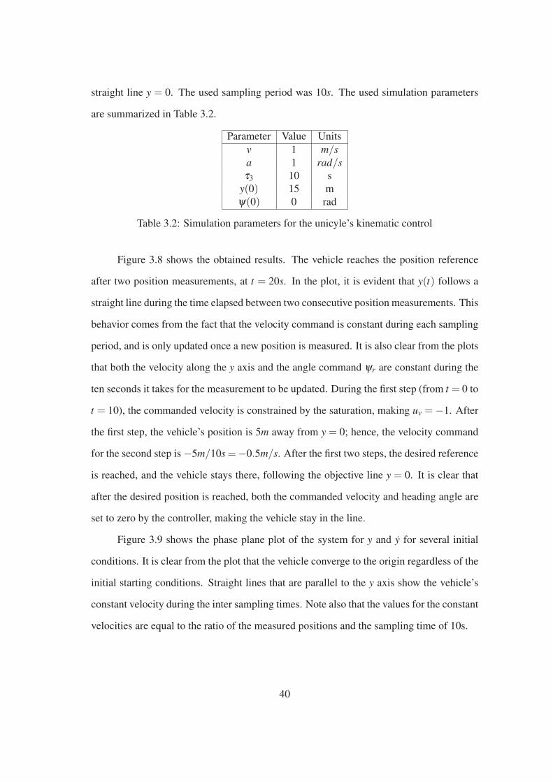
straight line y = 0. The used sampling period was 10s. The used simulation parameters

are summarized in Table 3.2.


v 1 m/s

a 1 rad/s

τ3 10 s

y(0) 15 m

ψ(0) 0 rad

Table 3.2: Simulation parameters for the unicyle’s kinematic control

Figure 3.8 shows the obtained results. The vehicle reaches the position reference

after two position measurements, at t = 20s. In the plot, it is evident that y(t) follows a

straight line during the time elapsed between two consecutive position measurements. This

behavior comes from the fact that the velocity command is constant during each sampling

period, and is only updated once a new position is measured. It is also clear from the plots

that both the velocity along the y axis and the angle command ψr are constant during the

ten seconds it takes for the measurement to be updated. During the first step (from t = 0 to

t = 10), the commanded velocity is constrained by the saturation, making uv =−1. After

the first step, the vehicle’s position is 5m away from y = 0; hence, the velocity command

for the second step is−5m/10s =−0.5m/s. After the first two steps, the desired reference

is reached, and the vehicle stays there, following the objective line y = 0. It is clear that

after the desired position is reached, both the commanded velocity and heading angle are

set to zero by the controller, making the vehicle stay in the line.

Figure 3.9 shows the phase plane plot of the system for y and y for several initial

conditions. It is clear from the plot that the vehicle converge to the origin regardless of the

initial starting conditions. Straight lines that are parallel to the y axis show the vehicle’s

constant velocity during the inter sampling times. Note also that the values for the constant

velocities are equal to the ratio of the measured positions and the sampling time of 10s.

40

Figure 3.8: Kinematic control simulation of the unicycle

3.4 Stability analysis and velocity of convergence

This section presents the stability analysis and velocity of convergence of the proposed

multirate control approach. The general system discussed in the first section of this Chap-

ter is used for this purpose, and the analysis applies to both case studies. The two case

studies presented in this chapter have a similar structure that allows splitting the control

tasks in subsystems. Each subsystem, represented by a loop, can have a different sampling

rate. The inner loops have the task of controlling an angle that will ultimately determine

41

Figure 3.9: Phase plane plot of the unicycle’s kinematic control

the velocity along an axis of displacement.

In the case of the unicycle, the forward velocity is considered constant, and a heading

angle changes the proportion of that speed along the y axis. In the case of the quadrotor,

the velocity is controlled indirectly by the attidude angles. The angles do not describe the

velocity along the axes of displacement directly, but indicate the orientation of the thrust

produced by the motors. The velocity is controlled by setting an appropriate behavior to

the attitude angles, such that the commanded velocity is reached. Once the velocity is

controlled, the vehicle can track waypoints using the proposed algorithm.

The main stability result is now stated.

Theorem: The position trajectories of systems (3.7) and (4.37) converge to the value up

after n+1 position sampling periods.

Proof:

Depending on the measured distance between the vehicle at t = k3τ3 and the position

42

reference up, three cases can occur:

Case 1: 3x(k3τ3)> up +uvτ3

This implies that

up−3x(k3τ3)

τ3<−uv. (3.37)

Hence, according to equations (3.14) and (3.13) in the case of the quadrotor and (3.30) for

the unicycle, uv =−uv. Then, from (3.20) and (3.36),

3x(k3τ3) =3x((k3 +1)τ3)+uvτ3. (3.38)

Replacing 3x(k3τ3) in inequality (3.37),

3x((k3 +1)τ3)+uvτ3 > up +uvτ3

3x((k3 +1)τ3) > up

(3.39)

Also, from 3.20, and since uvτ3 is strictly positive,

3x((k3 +1)τ3)<3x(k3τ3). (3.40)

In consequence,

up <3x((k3 +1)τ3)<

3x(k3τ3) (3.41)

Case 2: 3x(k3τ3)< up−uvτ3

Following the same analysis as in Case 1, it is clear that uv = uv, implying that

3x(k3τ3) =3x((k3 +1)τ3)−uvτ3. (3.42)

Replacing 3x(k3τ3) in inequality (3.37),

43

3x((k3 +1)τ3)−uvτ3 < up−uvτ3

3x((k3 +1)τ3) < up.(3.43)

Since uvτ3 is strictly positive, it is also clear that

3x((k3 +1)τ3 >3x(k3τ3). (3.44)

It yields

up >3x((k3 +1)τ3)>

3x(k3τ3) (3.45)

Case 3: up−uvτ3 ≤3x(k3τ3)≤ up +uvτ3

Under this condition, from equations (3.14) and (3.13), it is found that

uv =up−

3x(k3τ3)

τ3. (3.46)

Implying that

3x((k3 +1)τ3) =3 x(k3τ3)+

up−3x(k3τ3)

τ3τ3, (3.47)

therefore,

3x((k3 +1)τ3) = up (3.48)

Equation (3.48) shows that if 3x(k3τ3) is contained in the region of Case 3, x1 con-

verges to up after only one sampling period. It will now be shown that if x1(0) is any

finite value, x1 will converge to the region of Case 3 in a finite and predictable number of

sampling periods. This will prove that the system converges to x1 = up in a finite number

of steps, regardless of the starting position.

Let n ∈ Z+ be an arbitrary number of sampling periods and 3x(nτ3) the vehicle’s

position after nτ3 seconds. From (3.38) and (3.42), it is evident that 3x(k3τ3) follows

44

an arithmetic sequence in the regions of Case 1 and Case 2, respectively. An arithmetic

sequence has the form

3x(nτ3) =3x(0)+n∆. (3.49)

An arithmetic sequence grows in uniform steps towards positive infinity if ∆ is pos-

itive, or grows towards negative infinity if ∆ is negative.

For Case 1, x1 will decrease until up < x1(nτ3)≤ up +uvτ3, getting in the region of

Case 3. Denoting ⌈·⌉ as the smallest positive number greater or equal than its argument,

and making 3x(nτ3) = up+uvτ3, from (3.49) and (3.38), the number of required sampling

periods to reach the region of Case 3 is

n =

⌈

x1(0)

uvτ3−1

⌉

(3.50)

Following the same reasoning, for Case 2, x1 will increase in uniform steps until

up > x1(nτ3)≥ up−uvτ3, getting also in the region of Case 3. From (3.49) and (3.42) and

making 3x(nτ3) = up−uvτ3,

n =

⌈

−x1(0)

uvτ3−1

⌉

(3.51)

As shown in (3.48), once x1 reaches the region of Case 3, it converges to up in

one additional sampling period. Furthermore, (3.15) and (3.9) shows that if x1 = up, also

uv = ua = 0; therefore, x2 = x3 = 0. This proves that the system converges to up and re-

mains there after n+1 sampling periods.

45

Chapter 4

Dynamics Control and Experimental

Results

This chapter discusses the dynamics control of the two case studies introduced in Chapter

3 using the proposed multirate control technique. Each system model is analyzed and

simulated, considering both its kinematics and dynamics. In addition to this, experimental

results obtained with the HYCONS Quadrotor and the HYCONS Rover are presented.

The results of this chapter clearly show that Assumptions Q2 and U1 are reasonable from

a practical point of view. It is shown that for most of the simulation time, Assumptions

Q2 and U1 are valid, and the short transient periods of time when they are not valid do

not have any influence in the steady state behavior of the closed-loop system. To motivate

future extensions of the work presented in this thesis, a brief analysis of the unicycle’s

control model using singular perturbations theory is discussed at the end of this chapter.

4.1 Quadrotor Helicopter

In the first part of this section, the dynamics component of the proposed multirate control

technique for the case of the HYCONS quadrotor helicopter is discussed. The dynamics

control, which is done in the attitude loop (see Figure 4.1), has the objective of making

46

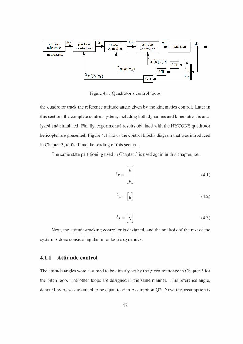
Figure 4.1: Quadrotor’s control loops

the quadrotor track the reference attitude angle given by the kinematics control. Later in

this section, the complete control system, including both dynamics and kinematics, is ana-

lyzed and simulated. Finally, experimental results obtained with the HYCONS quadrotor

helicopter are presented. Figure 4.1 shows the control blocks diagram that was introduced

in Chapter 3, to facilitate the reading of this section.

The same state partitioning used in Chapter 3 is used again in this chapter, i.e.,

1x =

θ

p

(4.1)

2x =[

u

]

(4.2)

3x =[

X

]

(4.3)

Next, the attitude-tracking controller is designed, and the analysis of the rest of the

system is done considering the inner loop’s dynamics.

4.1.1 Attidude control

The attitude angles were assumed to be directly set by the given reference in Chapter 3 for

the pitch loop. The other loops are designed in the same manner. This reference angle,

denoted by ua was assumed to be equal to θ in Assumption Q2. Now, this assumption is

47

no longer used, and an attitude angle tracking controller is designed. It will be later shown

that the system behaves very similarly when the assumption is made and when the angle

is tracked by the attitude controller.

As stated before, three different controllers per horizontal axis (X, Y) must be de-

signed to stabilize the system using the proposed multi-rate control technique. Every time

a new position sampling is made, the position control computes the constant speed required

to get to the reference position after τ3 seconds. If the magnitude of this required speed is

greater than the vehicle’s maximum speed |uv|, this maximum speed is commanded. The

velocity controller commands the attitude angles so that the speed given as reference by

the position controller is achieved and maintained.

Remark: In principle, intuition leads to think that as long as the angles converge fast

enough to the given reference ua, any controller can be implemented to track the atti-

tude reference and the overall system will still be stable and converge to the commanded

position.

Attitude angles are small during non-aggressive maneuvers. Hence, linear con-

trollers can be used for the attitude loop. Following the approach used in Chapter 3,

one of the axis of displacement is isolated to help the illustration of the proposed multirate

control technique. From equation (3.3), the dynamics of the attitude angle are

θ = p

p = u3/Iyy

(4.4)

We now design u3 using a pole-placement procedure in such a way that θ tracks its

reference, ua with an overshoot of 1% and a settling time of 0.25s.

As stated before, θ and p are sampled with a period of τ1. The sampled sub state

vector 1x is denoted by

48

1x(k1τ1) =

θ(k1τ1)

p(k1τ1)

. (4.5)

A state feedback controller is designed for the pitch control as

u3 = ka(~ua−1x(k1τ1)) (4.6)

where

ka =[

1 0.09

]

(4.7)

and

~ua =

ua

0

(4.8)

Hence, the closed-loop attitude-tracking system is

θ = p

p =ka

Iyy(~ua−

1x(k1τ1))(4.9)

Figure 4.2 shows a simulation of the designed attitude-tracking controller in equa-

tion (4.9). Table 4.1 summarizes the parameters used in the simulation. The time-response

follows the design criteria; the settling time is 0.25s and the overshoot is about 1%.


τ1 13.2 ms

1/Iyy 322 kg/m2

ua π/4 rad

x3(0) 0 rad

x4(0) 0 rad/s

Table 4.1: Simulation parameters for the attitude-tracking controller simulation

The used sampling period τ1 was chosen to be equal to the one provided by the

implemented sensor and network (76Hz), which yields a sampling period of 13.2ms. It is

now proven that the attitude stabilization system is stable for this sampling rate.

49

Figure 4.2: Attitude-tracking controller simulation

The attitude-tracking control is a linear system that can be written in the form

x(t) = Ax(t)+Bu(t), (4.10)

For which a continuous-time linear controller of the form

u(t) = Kx(t) (4.11)

can be designed.

Assumption 4.1.1. The measurements for computing the control input are taken in a

50

sample-and-hold fashion. Therefore, the control input can be rewritten as

u(t) = Kxtn , for t ∈ [tn, tn+1), (4.12)

where tn and tn+1, n ∈ N, are two consecutive sampling times, and xtn = x(tn).

We denote the time elapsed since the last sampling instant by

ρ(t) = t− tn, for t ∈ [tn, tn+1), (4.13)

and the longest interval between two consecutive sampling times by τ , i.e,

τ = supn∈N

(tn+1− tn). (4.14)

We denote the m×m identity matrix by Im.

The next theorem follows from the results of [59], and provides a set of linear matrix

inequalities which guarantee that the sampled-data linear system asymptotically converges

to the origin.

Theorem 4.1.1. Consider the closed-loop sampled-data linear system defined in (4.10)

and (4.12) with sampling intervals smaller than τ . The system is asymptotically stable to

the origin if there exist symmetric positive definite matrices P, R, and X, and matrix N

with appropriate dimensions, satisfying

Ψ+ τ(M1 +M2)< 0 (4.15)

Ψ+ τ(M2 +M3) τN

τNT − τR

< 0 (4.16)

where

Ψ =

AT

KT BT

[

P 0

]

+

P

0

[

A BK

]

51

−

Inx

−Inx

X[

Inx− Inx

]

−

Inx

−Inx

NT −N[

Inx− Inx

]

,

M1 =

AT

KT BT

X[

Inx− Inx

]

+

Inx

−Inx

X[

A BK

]

,

M2 =

AT

0

R[

A 0

]

,

M3 =

0

KT BT

NT +N[

0 BK

]

.

The proof of this theorem can be found in [59]. Based on Theorem 4.1.1, the prob-

lem of finding the longest interval between two consecutive sampling times that preserves

asymptotic stability is formulated as

Problem 4.1.1.

maximize τ

subject to P > 0, R > 0, X > 0, (4.15)− (4.16).

We denote the solution of Problem 4.1.1 by τmax. Using the system’s characteristics,

τmax is found to be 154ms.

This result, further explained in [60] is based on a Lyapunov-Krasovskii functional.

The found upper bound for the maximum allowable sampling period was found to be

154ms, which is far higher than 13.16ms. Therefore, stability of the attitude loop is guar-

anteed (see [60] for more details).

Now, with this attitude-tracking controller, the velocity controller shown in Chap-

ter 3 can be implemented, no longer using the Assumption Q2, and validating that this

assumption is reasonable form a practical point of view. The velocity and position con-

trollers that were designed in Chapter 3 are analyzed in the following subsections, taking

into account the attitude angle dynamics.

52


The same velocity controller that was designed in Chapter 3 is now implemented in model

(3.3), considering the attitude dynamics. The velocity controller that was shown in equa-

tion (3.9) is used:

ua =M

u1kv(uv−

2x(k2τ2)). (4.17)

Using (4.6), the model described in equation (3.3) is transformed into

X = u

u = u1/M sinθ

θ = p

p =ka

Iyy

M

u1kv(uv−

2x(k2τ2))

0

− 1x(k1τ1)

(4.18)

where ka is given by equation (4.7) and 1x(k1τ1) and 2x(k2τ2) are given by (4.1, 4.2).

The velocity-tracking simulation results are shown in subsection 4.1.4, together with

the attitude and position tracking. It will now be shown that the system converges to up.


As in the previous subsection, the position controller that was discussed and designed in

Chapter 3 is now implemented in model (3.3), considering the dynamics of the attitude

angle. Replacing uv in (4.18) by the velocity controller shown in equation (3.15), the

closed-loop model takes the form

53

X = u

u = u1/M sinθ

θ = p

p =ka

Iyy

M

u1kv

[

sat

(

up−3x(k3τ3)

τ3

)

− 2x(k2τ2)

]

0

− 1x(k1τ1)

(4.19)

where up is desired position reference. Equation (4.19) is the model of a PWA control

system for which the tools presented in [62] could be extended in future work and then

used to analyze stability. Note that the input u3 to θ takes an interesting form due to the

different rates at which the state measurements are made. The three portions of the state

are interacting in the same expression, and being updated at different rates. The inner

round brackets, where the position input is computed, is updated every τ3 seconds. Until

the next position measurement is done, the velocity commands are computed in the square

bracket at a rate of 1/τ2Hz. In turn, this velocity input sets the reference to the attitude-

tracking controller, which is computed every τ1 seconds. The combination of these three

inputs at different rates, produces the necessary commands to motors 2 and 4, so that the

quadrotor’s pitch angle envelope has an appropriate shape that makes the vehicle track a

given position reference up in the X axis. The simulation results are shown in the next

subsection.


System (4.19) was simulated using the parameters shown in Table 4.2. Both dynamics and

kinematics are considered in this simulation. The Assumption Q2, made on Chapter 3 for

the attitude angle is removed, and the attitude-tracking controller discussed in Subsection

4.1.1 is used instead. As in Chapter 3, the position sampling period (τ3) is 10s and the

given position reference up = 5m. The sampling period for 2x and 1x is again based on

MicroStrain 3DX-GM IMU, τ2 = τ3 = 13.2ms.

54

Figure 4.3: Dynamics control simulation of the HYCONS quadrotor model

The obtained results are shown in Figure 4.3. As in Figure 3.5, The quadrotor

reaches the given position reference in 3τ3 seconds, at t = 30s. The trajectory described

by X is a straight line between two sampling periods due to the constant velocity reference

that is given by the position controller. It can be noted that the velocity is tracked as fast as

in the kinematics simulation shown in Chapter 3, although the angle is no longer assumed

to be directly accessible as a control input, and an attitude-tracking controller is used in-

stead. This confirms the effectiveness of the proposed multirate control technique and the

fact that Assumption Q2 is reasonable from a practical point of view. Refer to Figure 3.5

55


u1/M 25 g−1

1/Iyy 322 m2/g

up 5 m

uv 0.2 m/s

τ1 13.2 ms

τ2 13.2 ms

τ3 10 s

kv .32

X(0) 0 m

u(0) 0 m/s

θ(0) 0 rad

p(0) 0 rad/s

Table 4.2: Parameters for the quadrotor’s dynamics control simulation

to verify the similarity of the two responses.

4.1.5 Experimental results

Figure 4.4 shows some experimental results obtained for the attitude stabilization control

loop. The plot shows the attitude angles and its rates of change during a short take-off,

hover and land flight. The roll and pitch angle references were set to zero; the yaw angle’s

rate of change was stabilized to zero by adding a damping input, since the magnetometer

implemented in the UAV does not provide reliable information indoors, due to the strong

electromagnetic interference that is present inside a building. It is evident from the plots

that the attitude angles are stabilized around zero, with small oscillations of about ±2deg.

Although some small oscillations are observed, the system remains stable during the ma-

neuver.

Due to technical limitations, the presented results are preliminary, and only show

the performance of the attitude control loop. The validation of the whole multirate control

technique is proposed as future work. For this purspose, new equipment must be used to

track the quadrotor’s position in space with a good reliability, precision and repeatability.

The acquisition of such equipment is being studied.

56

Figure 4.4: Experimental results obtained with the HYCONS Helicopter

4.2 Unicycle

The first part of this section addresses the rotational dynamics control of the unicycle. This

component of the vehicle’s control, is done in the inner loop of the proposed multirate

system. This component has the task of making the heading angle track the reference

signal that is given by the velocity controller. Later in this section, the analysis of the

velocity and position loops is made, considering the rotational dynamics and the respective

simulations are presented. It will be shown that the behavior of the system under the

mentioned assumption is very similar to the one without the assumption, where the heading

57

angle reference is tracked by a controller. Finally, experimental results obtained with the

HYCONS rover are presented.

The same partitioning of the state vector that was used in Chapter 3 is considered

here:

1x =[

ψ

]

(4.20)

2x =[

y

]

(4.21)

3x =[

y

]

(4.22)

The heading-tracking control is now addressed.

4.2.1 Heading angle tracking control

In Chapter 3, the heading angle, ψ , was assumed to be directly set by the reference ψr in

Assumption U1. This is now removed, and a heading-tracking controller is designed and

implemented instead. In subsection 4.2.4 it will be shown that the response is very similar

in the cases when the assumption is made and when the heading controller is used.

Considering only the rotational dynamics of equation (3.21),

ψ = au. (4.23)

Using a state feedback controller, and noting that the sampled values of ψ are

1x(k1τ1), we make

u = kψ(ψr−1x(k1τ1)), (4.24)

where ψr is the reference given to the inner control loop and kψ is an appropriate feedback

gain. Using (4.24), equation 4.23 can be rewritten as

58

ψ = akψ(ψr−1x(k1τ1)) (4.25)

which is a heading-tracking linear controller. The model of the unicycle, including the

heading-tracking control rotational dynamics in (4.25), can then be written as

y = vsin(ψ)

ψ = akψ(ψr−1x(k1τ1))

(4.26)

The velocity control is addressed in the next subsection, and the heading angle ref-

erence, ψr is designed.


As discussed in section 3.3.1, the velocity loop does not have dynamics with respect to

the rotational dynamics. The exact same relationship found in Chapter 3 is used here to

compute the heading reference ψr based on the position control output uv. This is

ψr = sin−1(uv

v

)

. (4.27)

Hence, the model (4.26) becomes

y = vsin(ψ)

ψ = akψ

[

sin−1(uv

v

)

− 1x(k1τ1)]

.(4.28)

In the next subsection, the input to system (4.28), uv, is designed.


In this subsection, the analysis addressed in Chapter 3 is extended, considering the rota-

tional dynamics of the unicycle. It was found that the velocity reference that is required

for y to converge to zero after τ3 seconds is

59

uv =− 3x(k3τ3)

τ3. (4.29)

Thus, the heading reference, according to equation (3.27) is

ψr = sin−1

[

sat

(

− 3x(k3τ3)

vτ3

)]

(4.30)

and the model takes the form

y = vsin(ψ)

ψ = akψ

sin−1

[

sat

(

− 3x(k3τ3)

vτ3

)]

− 1x(k1τ1)

(4.31)

Equation (4.31) is the model of a PWA control system. It is worth noting the form

that the input u takes here due to the different sampling rates that are present in the control

system. The two partitions of the state space that are being measured are updated at differ-

ent rates. The expression inside the curly brackets is updated every τ1 seconds, based on

the most recent value of 3(k3τ3), that is only updated every τ3 seconds and held constant

until a new measurement is made.

These two inputs that are being updated at different rates are combined in such way

that u is commanded to produce a heading angle envelope that makes the unicycle follow

the straight line y = 0. Some simulation results are presented in the next subsection.


The system (4.31) was simulated to test the performance of the proposed multirate control

technique. For those parameters that are common to the simulations in Chapter 3 and

the one presented in this section, the same values are used. Table 4.3 summarizes the

parameters used in the simulation. As stated before, the control task is to follow the

straight line y = 0.

The obtained simulation results are shown in Figure 4.5. The unicycle converges to

y= 0 after two position measurement periods; this is, t = 20s. In a very similar way to what

60


v 1 m/s

a 1 rad/s

τ1 0.04 s

τ3 10 s

y(0) 15 m

ψ(0) 0 rad

Table 4.3: Simulation parameters for the unicyle’s dynamics control

was shown in the kinematic control simulation results, the trajectory of y(t) between two

consecutive sampling times is a straight line, indicating that the velocity is constant. This

fact is evident in the plot of y, where the given reference is constant and the state tracks

it in a small portion of τ3. Note that in this simulation, where the rotational dynamics

are included, the angle is no longer assumed to be directly accessible as input. Instead, a

heading-tracking controller generates the appropriate signal u such that ψ converges fast

to ψr. It is possible to see in the plot that the time it takes for ψ to converge to ψr is very

small compared to τ3, because of the difference in speed of the different state variable’s

dynamics. This shows the efficiency of the proposed multirate control technique. It is

also possible to note that during from t = 0 to t = 10, the commanded velocity is kept

constrained by the saturation, hence uv =−1. The vehicle’s position is 5m away from y= 0

in t = 20s; therefore, the velocity command for the second step is −5m/10s = −0.5m/s.

After the first two steps, the desired reference is reached, and the vehicle stays there,

following the objective line y = 0. It is clear that after the desired position is reached, both

the commanded velocity and heading angle are set to zero by the controller, making the

vehicle stay in the line.

A phase plane plot of the system is shown in Figure 4.6 for y and y. Several initial

conditions are considered. Similarly to what was shown in the phase plane plot in Chapter

3, the vehicle converges to the origin regardless of the initial starting conditions. If Figure

4.6 is carefully compared to Figure 3.9, small differences can be found in the shape of the

trajectories. This small differences are caused by the short time it takes for y to converge

61

Figure 4.5: Unicycle dynamics simulation results

to uv, that was assumed to be zero in Chapter 3.

4.2.5 Experimental results

Two experiments were performed using the HYCONS Rover. Table 4.4 summarizes the

parameters that are common to both experiments. It is worth noting that the experiments

were performed using the vision tracking system that was described in Chapter 1. There-

fore, the distance units used in this subsection are camera pixels. The velocities along

the y axis, however, are normalized with respect to the forward speed v, mapping it in the

62

Figure 4.6: Phase plane plot of the unicycle’s dynamics control

interval [−1,1].


v 6.2 px/s

a 1 rad/s

kψ 5 —

τ1 40 ms

τ3 5 s

Table 4.4: HYCONS Rover experiment’s parameters

In the first experiment, shown in Figure 4.7, the vehicle’s initial position is y= 220px

and its heading is ψ = 0.11rad. After the command up = 150 is given at t = 5s, the

commanded normalized velocity uv is −1, which is its maximum value allowed by the

saturation. This value provides a heading reference of ψr = −π/2. This reference is

achieved in approximately 2s. Subsequently, velocity and heading references are given

every 5s, when a new position is measured, making the vehicle’s position converge to the

reference in roughly 15s after the position reference is given. Although some noise from

63

Figure 4.7: Experimental results obtained with the HYCONS Rover

the measurements is evident, the performance closely resembles the simulations, showing

the robustness and practical relevance of the proposed multirate control technique.

The second experiment, shown in Figure 4.7 has different initial conditions. The

vehicle’s initial position is y = 56px and its initial heading is ψ = 0.06rad. The position

reference is again uv = 150px, which is reached roughly after 15s, as in the first experi-

ment.

For both experiments, it is possible to see that the system behaves very closely to

what the simulations showed. Straight trajectories are clearly observed between sampling

64

Figure 4.8: Further experimental results obtained with the HYCONS Rover

times, since constant velocities and heading references are given during such time inter-

vals. The heading angle and velocity converges to the given references in a portion of the

sampling period for position, τ3. The implemented machine vision system has a rather

low resolution compared to the HYCONS Rover’s workspace; the resolution is of about

109px/m, and therefore the feedback was affected by quantization error, and noise. The

presented results were slightly filtered, using a moving average, to make the curves clear

to the reader.

Next, a brief analysis of the Unicycle’s control system is presented as a motivation

to future work. It also provides an intuitive justification for Assumption U1.

65

4.2.6 Singular perturbations analysis

Singular perturbations analysis provides a theoretical foundation to the engineering practi-

cal approach of neglecting some terms of a system’s model when they are considered to be

small compared to the other magnitudes involved. In dynamical systems, this is relevant

when multiple time scales are involved in a model, yielding ”slow” and ”fast” dynamics.

The analysis presented in this subsection is based on [63].

Let us recall equation (3.21), which describes the dynamics of the unicycle model,

y = vsin(ψ)

ψ = au

(4.32)

By using a continuous time linear controller to track a reference heading, we make

u = kψ(ψr−ψ) (4.33)

and the system (3.21) becomes

y = vsin(ψ)

ψ = akψ(ψr−ψ). (4.34)

By letting

ε =1

akψ, (4.35)

we can rewrite system (4.34) as

y = vsin(ψ)

εψ = ψr−ψ

(4.36)

As akψ is made very large, then ε → 0 and (4.36) can be analyzed as a singularly

perturbed system. When ε = 0, neglecting the dynamics of the attitude control loop, the

second line of equation (4.36) becomes the algebraic expression: ψ = ψr, and the system

(4.36) reduces to

66

y = vsin(ψr) (4.37)

which is exactly the Assumption U1, made in Chapter 3 and later removed in Chapter 4,

where a heading-tracking controller was designed and this dynamics were considered in

the analysis and simulations.

By comparing closely Figures 3.9 and 4.6, it is possible to see only very small dif-

ferences in the trajectories of the states as a consequence of neglecting or considering the

system’s fast dynamics. Also, by carefully comparing Figures 3.8 and 4.5, it is possi-

ble to see small differences in the shapes of the curves, especially when a new position

measurement is made, and new velocity and angle commands are computed. These two

examples clearly show how the singularly perturbed system is an approximation of the

original model.

67

Chapter 5

Conclusions

The main conclusions of this thesis are summarized in this final chapter, based on the

contributions stated in Chapter 1. Potential future extensions of the work presented on this

thesis are also proposed.

In Chapter 2, the conception, design and construction process was described, and

a nonlinear model was presented. The vehicle was successfully designed and built, and

its performance was satisfactory during both preliminary tests on ground and final flight

tests. The attitude-tracking controller can stabilize the aircraft, allowing it to hover and

navigate in indoor environments. Several different upgrades could be made to extend the

capabilities of the HYCONS Quadrotor; however, the two following are proposed as the

most immediate:

• Add a position-tracking sensor or system to the vehicle, and

• add environment ranging sensors.

With the addition of a position tracking system, the vehicle would be able to navigate

completely autonomously in an environment, provided there are no obstacles in the com-

manded positions and possible trajectories. For indoor navigation, a tracking system based

on infrared cameras is proposed. For outdoor navigation, a Global Positioning System

(GPS) is proposed. On the other hand, environment ranging sensors would allow the

68

quadrotor to navigate in an environment even if there are obstacles in it, avoiding colli-

sions and exploring different paths to complete a navigation control task.

In Chapter 3, the kinematics control of proposed multirate technique was discussed.

It was shown in both analysis and simulation that the proposed approach successfully con-

trols the two presented case studies under the assumption of directly controllable head-

ing/attitude angles. For both case studies, the velocity along the axis of interest was shown

to be controllable by modifying the heading/attitude angles. The velocity-controlled ve-

hicle was shown to converge in a predictable number of steps to the commanded position

under an arbitrarily low sampling frequency for the position loop. The following exten-

sions are proposed as future work:

• Different paths that might take the vehicle faster to the commanded position can be

explored, instead of using constant velocity commands that yield straight trajecto-

ries,

• Inter-sampling position estimation can be made based on the information from other

states, the control inputs and a model.

The dynamics control was addressed in Chapter 4. The assumption of directly con-

trollable heading/attitude angles was removed, and the analysis was carried out consid-

ering the rotational dynamics for both case studies. Angle-tracking controllers were de-

signed to meet specific performance requirements that guarantee the overall stability of the

proposed multirate system. The complete closed-loop system was derived and simulations

for both case studies were performed, showing that the behavior of the angle-controlled

system is very similar to the behavior of the systems under the assumptions made on

Chapter 3. Experimental results were also presented, showing a performance that closely

resembles the behavior that was expected from the simulations. The following extensions

are proposed for future work:

• Formalize the conditions under which the dynamical system is guaranteed to be

69

stable without the assumptions made in Chapter 3 (Assumptions Q2 and U1).

• Extend the experimental results with a positioning system to perform fully autonomous

navigation tests.

70

Bibliography

[1] J. N. Yelverton, ”Wireless Avionics”, Digital Avionics Systems Conference, 1995. 14th DASC. MA,

USA, 1995.

[2] W. Kim, J. Biesiadecki, and K. Ali, ”Visual Target Tracking on the Mars Exploration Rovers”, Inter-

national Symposium on Artificial Intelligence, Robotics and Automation in Space, CA, USA, 2008.

[3] P. Castillo, R. Lozano. A. Dzul, ”Modelling and control of mini-flying machines”. Springer, 2005.

[4] Adapted from the Wikimedia Commons file ”Image:De Bothezat Quadrotor.jpg”, URL:

[5] J. Boreinstein, ”The HoverBot, An Electrically Powered Flying Robot” Unpublished White paper,

University of Michigan, USA, 1992.

[6] I. Kroo, F. Prinz, et al, ”The Mesicopter: A Miniature Rotorcraft Concept”, Stanford University, USA,

2000.

[7] E. Altug, J.P. Ostrowski, R. Mahony, ”Control of a quadrotor helicopter using visual feedback”, Pro-

ceedings of the International Conference on Robotics and Automation, Washington DC, USA, 2002.

[8] A. Moktari, A. Benallegue, ”Dynamic Feedback Controller of Euler Angles and Wind Parameters Es-

timation for a Quadrotor Unmanned Aerial Vehicle”, Proceedings of the IEEE Conference on Robotics

and Automation, 2004.

[9] A. Benallegue, A. Moktari, L. Friedman, ”Feedback Linearization and High Order Sliding Mode

Observer for a Quadrotor UAV”, Proceedings of the International Workshop on on Variable Structure

Systems, 2006.

[10] J. Dunfried, M. Tarbouchi, G. Labonte, ”Neural Network Based Control of a Four Rotor Helicopter”,

Proceedings of the IEEE International Conference on Industrial Tecnhology, 2004.

71

[11] A. Tayebi, S. McGilvray, ”Attitude Stabilization of a VTOL Quadrotor Aircraft”, IEEE Transactions

on Control Systems Technology, vol. 14, No. 3, May, 2006.

[12] K. Alexis, C. Papachristos, G. Nikolakopoulos, A. Tzes, ”Model predictive quadrotor indoor position

control”, 19th Mediterranean Conference on Control and Automation, Corfu, Greece, 2011.

[13] J. Wang, T. Bierling, L. Hocht, F. Holzapfel, ”Novel Dynamic Inversion Architecture Design for

Quadrocopter Control”, Advances in Aerospace Guidance, Navigation and Control, Springer Berlin

Heidelberg, 2011.

[14] L.R. Garcia-Carrillo, E. Rondon, A. Dzul, A. Sanche, R. Lozano, ”Hovering quad-rotor control: A

comparison of nonlinear controllers using visual feedback”, 49th IEEE Conference on Decision and

Control, Atlanta, GA, USA, 2010.

[15] G.V. Raffo, M.G. Ortega, F.R. Rubio, ”An integral predictive nonlinear H-infinity control structure

for a quadrotor helicopter”, Automatica 46, 2010.

[16] J. Toledo, L. Acosta, M. Sigut, J. Felipe, ”Stabilisation and altitude tracking of a four-rotor microhe-

licopter using the lifting operators”, IET Control Theory and Applications, Volume 3, issue 4, 2009.

[17] ”ETH - IDSC - Flying Machine Arena.” ETH. Web. 16 Apr. 2012. URL:

[18] D. Mellinger, N. Michael, V. Kumar, ”Trajectory generation and control for precise aggressive ma-

neuvers with quadrotors”, International Journal of Robotics Research (Published online before print,

doi: 10.1177/0278364911434236, January 25, 2012.

[19] H. Huang, G. Hoffmann, S. Waslander, C. Tomlin, ”Aerodynamics and control of autonomous quadro-

tor helicopters in aggressive maneuvering”, Proceedings of the IEEE International Conference on

Robotics and Automation, ICRA ’09, 2009.

[20] M. Muller, S. Lupashin, R. D’Andrea, ”Quadrocopter Ball Juggling”, IEEE/RSJ International Con-

ference on Intelligent Robots and Systems, 2011.

[21] M. Hehn, R. D’Andrea, ”Quadrocopter Trajectory Generation and Control”, IFAC World Congress,

2011.

[22] S. Lupashin, R. D’Andrea, ”Adaptive Open-Loop Aerobatic Maneuvers for Quadrocopters”, IFAC

World Congress, 2011.

72

[23] A. Schoellig, M. Hehn, S. Lupashin, R. D’Andrea, ”Feasible Periodic Motion Primitives for Chore-

ographed Quadrocopter Flight”, American Control Conference (ACC), 2011.

[24] M. Hehn, R. D’Andrea, ”A Flying Inverted Pendulum”, IEEE International Conference on Robotics

and Automation, 2011.

[25] P. Wiberg, U. Bilstrup, ”Wireless technology in industry-applications and user scenarios”, Proceed-

ings of the 8th IEEE International Conference on Emerging Technologies and Factory Automation,

2001.

[26] R. Macedo, P. Carvalhal, J. Afonso, L. Silva, H. Almeida, M. Ferreiral, C. Santos, ”A Fly-By-Wireless

UAV Platform Based on a Flexible and Distributed System Architecture”, IEEE International Confer-

ence on Industrial Technology, 2006.

[27] P. Carvalhal, M. Ferreira, L. Silva, H. Almeida, C. Santos, J. Afonso, ”A Bluetooth-based Wireless

Distributed Data Acquisition and Control System”, IEEE International Conference on Robotics and

Biomimetics, 2006.

[28] R. Yedavalli, R. Belapurkar, ”Application of wireless sensor networks to aircraft control and health

management systems”, Journal of Control Theory and Applications, volume 9, issue 1, 2011.

[29] H. Liu, ”Aircraft wireless sensor network for in-flight fault diagnostics and control”, 3rd Annual

IEEE/CANEUS Fly by wireless Workshop, Orono, ME, USA, 2010.

[30] N. Taajwar, S. Faruque, ”Fly-By-CDMA wireless and single wire-line technology, a potential solution

for Fly-By-Wireless/Less-wire”, 4th Annual IEEE/CANEUS Fly by wireless Workshop, Montreal,

Canada, 2011.

[31] T. Upal, S. Faruque, ”Fly by wireless: An ultrasonic approach for UAV”, 4th Annual IEEE/CANEUS

Fly by wireless Workshop, Montreal, Canada, 2011.

[32] O. Elgezabal, C.Salazar, ”Technological foundation for future intra-aircraft wireless applications:

State of the art of wireless data transmission”, 4th Annual IEEE/CANEUS Fly by wireless Work-

shop, Montreal, Canada, 2011.

[33] S. Chilakala, Development and Flight Testing of a Wireless Avionics Network Based on the IEEE

802.11 Protocols. MSc Thesis, University of Kansas, 2008.

[34] D. Hope, ”Towards a Wireless Aircraft”, PhD Thesis, University of York, UK, 2011.

73

[35] G. Kranc, ”Input-output analysis of multirate feedback systems”, IRE Transactions on Automatic

Control, Volume 3, Issue 1, 1957.

[36] B. Friedland, ”Sampled-data control systems containing periodically varying members”, Proceedings

of the 1st IFAC Congress, 1960.

[37] J. Johnson, C. Phillips, ”Maximum errors from quantization in multirate digital control systems”,

AIAA Journal, American Institute of Aeronautics and Astronautics, Vol. 8, No. 4, 1970.

[38] D. Flowers, J. Hammond, ”Simplification of the characteristic equation of multirate sampled data

control systems”, IEEE Transactions of Automatic Control, Vol. 17, Issue 2, 1972.

[39] W. Boykin, B. Frazier, ”Multirate sampled-data systems analysis via vector operator”, IEEE Transac-

tions of Automatic Control, Vol. 20, Issue 4, 1975.

[40] D. Flowers, ”Design techniques for a class of multirate sampled data control systems”, Doctoral

Thesis, Georgia Institute of Technology, 1972.

[41] A. Tangirala, D. Li, R. Patawardhan, S. Shah, T. Chen, ”Ripple-free conditions for lifted multirate

control systems”, Automatica, Volume 37, Issue 10, 2001.

[42] H. Fijumoto, Y. Hori, A. Kawamura, ”Perfect tracking control based on multirate feedforward control

with generalized sampling periods”, IEEE Transactions on Industrial Electronics, Volume 48, Issue 3,

2001.

[43] L. Yang, S. Yang, ”Multirate Control in Internet-Based Control Systems”, IEEE Transactions on

Systems, Man, and Cybernetics, Part C: Applications and Reviews, Volume 37, Issue 2, 2007.

[44] H. Fujimoto, ”Visual servoing of 6 DOF manipulator by multirate control with depth identification”,

Proceedings of the IEEE Conference on Decision and Control, 2003.

[45] S. Brittanti, F. Dell’Orto, A. Di Carlo, S. Savaresi, ”Notch filtering and multirate control for radial

tracking in high-speed DVD-players”, IEEE Transactions on Consumer Electronics, Volume 48, Issue

1, 2002.

[46] Digi International Inc, ”Digi XBee Wireless RF Modules”.

URL: http://www.digi.com/xbee/

74

[47] DIY Drones, ”XBee - Discussion forums - DIY Drones”.

URL: http://diydrones.ning.com/forum/topic/listForTag?tag=xbee

[48] RC Groups, ”Quadricopter with UDB4+GPS+XBee - RC Groups”.

URL: http://www.rcgroups.com/forums/showthread.php?t=1590088

[49] Arduino Project Website, ”Arduino Mega Board”.

URL: http://arduino.cc/en/Main/ArduinoBoardMega

[50] MicroStrain Inc, ”3DM-GX1 Product Datasheet”.

URL: http://files.microstrain.com/3DM-GX1%20Datasheet%20Rev%201.pdf

[51] Castle Creations Inc, ”Thunderbird Brushless Motors Controls”.

URL: http://www.castlecreations.com/products/thunderbirds.html

[52] MaxBotix Inc, ”MB1040 LV-MaxSonar-EZ4 Ultrasonic Rangefinder”

URL: http://www.maxbotix.com/products/MB1040.htm

[53] Simulink Block by Sergey Shapovalov, ”RTsync Blockset - File Exchange - MATLAB Central”

URL: http://www.mathworks.com/matlabcentral/fileexchange/24975-rtsync-blockset

[54] Open Source Computer Vision - OpenCV Website. URL: http://opencv.willowgarage.com

[55] Horizon Hobby, ”Park 370 Brushless Outrunner Motor, 1360Kv (EFLM1205): E-flite - Advancing

Electric Flight”.

URL: http://www.e-fliterc.com/Products/Default.aspx?ProdID=EFLM1205

[56] S. Bouabdallah, R. Siegwart, ”Full Control of a Quadrotor”, Proceedings of the 2007 IEEE/RSJ Inter-

national Conference on Intelligent Robots and Systems, San Diego CA, USA, 2007

[57] K. Ogata, ”Modern Control Engineering, 5th ed.”, Prentice Hall, 2010.

[58] T. Bresciani, Modelling, Identification and Control of a Quadrotor Helicopter. MSc Thesis, Depart-

ment of Automatic Control, Lund University, Sweden, 2008.

[59] M. Moarref, L. Rodrigues, ”Asymptotic stability of piecewise affine systems with sampled-data piece-

wise linear controllers”, Proceedings of the 50th IEEE Conference on Decision and Control, FL, USA,

2011.

75

[60] C. Ossa-Gomez, M. Moarref, L. Rodrigues, ”Design, Construction and Fly-By-Wireless Control of an

Autonomous Quadrotor Helicopter”, Proceedings of the 4th IEEE / CANEUS Fly-by-wireless Work-

shop, Montreal, QC, Canada, 2011.

[61] C. Ossa-Gomez, L. Rodrigues, ”Multi-Rate Sampled-Data Control of a Fly-by-wireless Autonomous

Quadrotor Helicopter”, Proceedings of the 25th IEEE Canadian Conference on Electrical and Com-

puter Engineering CCECE’2012, Montreal, QC, Canada, 2012.

[62] L. Rodrigues, S., P., Boyd, ”Piecewise-affine state feedback for piecewise-affine slab systems using

convex optimization.”, Systems & Control Letters, 54(9), 835–853, 2005.

[63] H. Khalil, Nonlinear Systems, 3rd ed. Prentice Hall, NJ, USA, 2002

76

Documents

Design, Construction and Control of a Quadrotor Helicopter ... · Design, Construction and Control of a Quadrotor Helicopter Using a New Multirate Technique Camilo Ossa-G omez´ A