DESIGN, FABRICATION, AND EXPERIMENTAL CHARACTERIZATION OF

A LARGE RANGE XYZ PARALLEL KINEMATIC FLEXURE MECHANISM

by

John Edward Ustick

A thesis submitted in partial fulfillment

of the requirements for the degree of

Master of Science

(Mechanical Engineering)

in The University of Michigan

2012

Advisor: Shorya Awtar, Assistant Professor of Mechanical Engineering

ii

ACKNOWLEDGMENTS

I would like to acknowledge the following persons who helped me grow tremendously

throughout my graduate experience, and without whom this thesis would not be

complete:

Shorya Awtar, Sc.D., for being far more than a mentor. He is the reason I pursued a

Master’s degree, and he has helped me through the ups and downs of graduate school

with endless support and advice.

Shiladitya Sen, for teaching me much of what I now know about flexures, as well as

providing a significant contribution to the hardware and intellectual content contained

within this thesis.

Gaurav Parmar, for providing much needed support in the lab.

Jason Quint and Adrienne Lemberger, for contributing to a large portion of the

conceptual hardware design and manufacturing.

The Precision Systems Design Lab, for being a family away from home.

The people in the machine shop, for teaching me the many techniques necessary to

produce all of my hardware.

My mom, dad, and sister, for providing endless support.

My friend, Chris Haddad, for helping with numerous revisions.

My fiancée, Leigh Flechsig, for always keeping my outlook positive and encouraging me

every step of the way.

iii

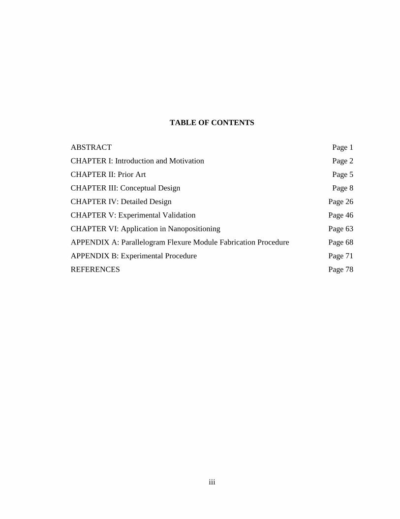
TABLE OF CONTENTS

ABSTRACT Page 1

CHAPTER I: Introduction and Motivation Page 2

CHAPTER II: Prior Art Page 5

CHAPTER III: Conceptual Design Page 8

CHAPTER IV: Detailed Design Page 26

CHAPTER V: Experimental Validation Page 46

CHAPTER VI: Application in Nanopositioning Page 63

APPENDIX A: Parallelogram Flexure Module Fabrication Procedure Page 68

APPENDIX B: Experimental Procedure Page 71

REFERENCES Page 78

1

ABSTRACT

A novel parallel kinematic flexure mechanism that provides highly decoupled motions along

the three translational directions (X, Y, and Z) and high stiffness along the three rotational

directions (Θx, Θy, and Θz) is presented. Geometric decoupling ensures large motion range

along each translational direction and enables integration with large-stroke ground-mounted

linear actuators or generators, depending on the application. The conceptual design is guided

by a constraint map, and qualitatively validated with two physical prototypes. The final

proposed design, which is based on a systematic arrangement of multiple rigid stages and

parallelogram flexure modules, is analyzed via non-linear finite elements analysis (FEA).

The analysis demonstrates an XYZ motion range of 10 mm x 10 mm x 10 mm. Over this

motion range, the non-linear FEA predicts cross-axis errors of less than 7.8%, parasitic

rotations less than 3.7 mrad, lost motion less than 14.4%, actuator isolation better than 1.5%,

and no perceptible motion direction stiffness variation. A prototype is fabricated to

experimentally validate the predicted large range and decoupled motion capabilities.

Experimental measurements demonstrate cross-axis errors of less than 11.6%, parasitic

rotations less than 6.98 mrad, lost motion less than 17%, actuator isolation better than 1.7%,

and no perceptible motion direction stiffness variation. Additionally, the mechanism is

integrated into a setup with non-contact sensors and actuators to demonstrate its application

in a nanopositioning system.

2

CHAPTER I

Introduction and Motivation

Flexure mechanisms derive motion from elastic deformation instead of employing traditional

sliding or rolling interfaces [1, 2]. This joint-less construction entirely eliminates friction,

wear, and backlash, leading to highly repeatable motion. Further benefits include design

simplicity, zero maintenance, and potentially infinite life [3].

By virtue of these attributes, flexure mechanisms are widely employed in various design

applications, in particular, multi-axis flexure mechanisms are used in precision alignment and

actuation instruments [39-40], micro-electro-mechanical system (MEMS) sensors and

actuators [31-32], energy harvesting devices [17], micro- and nano-manipulators [24], high

dexterity medical devices [41], scanning probe systems for precision metrology and

nanomanufacturing [42], as well as consumer products [43].

Multi-axis functionality may be achieved either via a serial kinematic [5-6] configuration or a

parallel kinematic [7-9] configuration. While a serial kinematic design may be simply

constructed by stacking one single-axis system on top of another to achieve the desired

degrees of freedom (DoF), such constructions are often bulky, complex, and expensive, due

in part to the need for moving cables and for actuators which adversely affect dynamic

performance. Parallel kinematic designs, on the other hand, employ ground-mounted

actuators and are often compact and simple in construction. Compared to serial kinematic

designs, their main drawbacks include smaller motion range, potential for over-constraint,

and greater error motions. Conceptually, synthesis of parallel kinematic designs is not

intuitive. The key objective is to overcome the above-mentioned traditional drawbacks in the

design of an XYZ parallel kinematic flexure mechanism.

The proposed concept is inherently free of geometric over-constraints, resulting in large

translational motions along the X, Y, and Z directions, and exhibits small error motions

(cross-axis errors and parasitic rotations). Large motion range along multiple axes is critical

in many applications, such as nanopositioning and kinetic energy harvesting, which in great

part motivated this work.

3

Nanopositioning systems are macro-scale mechatronic motion systems capable of nanometric

precision, accuracy, and resolution [10], and are therefore vital to scanning probe based

microscopy, manipulation, and manufacturing [11-12]. Given the lack of friction and

backlash, flexure mechanisms are the most common bearing choice for nanopositioning

systems. However, most existing flexure-based multi-axis nanopositioning systems are

capable of approximately a 100 µm range of motion per axis (see Prior Art section in

Chapter II). To broaden the impact of scanning probe techniques in nanometrology and

nanolithography requires a several fold increase this motion range [13-15]. The challenge

here is not only in the creation of a multi-axis flexure mechanism that is capable of large

motion range, but also in the mechanical integration of the flexure mechanism with ground-

mounted actuators.

Since flexure mechanisms incorporate the motion guidance attributes of mechanisms with the

elastic attributes of structures, they are also highly suited for energy harvesting schemes

based on a resonant proof mass subject to cyclic inertial loads. Even though the excitation,

and therefore the available energy, is generally in multiple directions, most energy harvesting

devices employ single axis resonators [16]. Given that the energy harvested is directly

proportional to the amplitude of oscillation [17], multi-axis flexure mechanisms with large

motion ranges could enhance efficient harvesting of kinetic energy. However, in addition to

providing a large range of motion in each direction, any candidate flexure mechanism must

also interface with fixed-axis generators for mechanical to electrical energy conversion.

In both nanopositioning and energy harvesting applications, a motion range of several

millimeters per axis would be desirable in a macro-size construction. Relevant fields in

nanopositioning include scanning probe microscopy [45-48], scanning probe

nanolithography [49], and chemical research such as molecular spectroscopy and drug

discovery [50]. Energy harvesting applications depend on resonance, with larger ranges

suitable for low frequency, high power applications [51].

This thesis covers the conception, analytical evaluation, and hardware validation of an XYZ

parallel kinematic flexure mechanism that meets the large-range motion requirement as well

as the pertinent actuator/generator integration challenges associated with these applications.

4

Chapter II lays out the design challenges in addition to providing a brief overview of the

existing literature on XYZ flexure mechanisms. Chapter III describes the conceptual design

process including the design and fabrication of preliminary prototypes. Chapter IV provides

the details of the final XYZ flexure mechanism design and its motion characteristics, as well

as a comprehensive non-linear finite element analysis. The predicted motion performance in

terms of motion range, cross-axis error, lost motion, parasitic rotations, and stiffness

variation is reported. Chapter V presents the experimental validation of the predicted motion

characteristics, including the design and fabrication an experimental setup. Chapter VI

presents an application of the flexure mechanism through the design and fabrication of a

nanopositioning setup. APPENDIX A discusses additional information regarding the flexure

mechanism fabrication procedure. APPENDIX B discusses additional information regarding

the experimental procedure.

5

CHAPTER II

Prior Art

The motion axes – X, Y, and Z – must be decoupled from each other so that motion in one

axis does not affect or constrain motion in the other axes. Motion range in multi-axis, parallel

kinematic mechanisms is often restricted due to over-constraint, typically resulting from a

geometric layout that creates coupling between the motion axes. This ultimately leads to

binding and restricts mobility.

Moreover, the undesirable parasitic rotations, rotations (i.e., x, y, and z) caused by other

inputs such as translations, should be inherently restricted and minimized by the kinematics

of the design. This eliminates the need for additional actuators, beyond the minimum three

needed for X, Y, and Z actuation, to correct these undesired rotations. In addition to

providing geometric decoupling between the three motion axes, which prevents each motion

direction from affecting the other motion directions, it remains important that the flexure

mechanism addresses the geometric constraints associated with integrating practically

available actuators or generators.

For an XYZ nanopositioning system, linear actuators are a simple solution that prevents the

need for any additional transmission. However, most linear actuators [18], including voice

coils, linear motors, piezoelectric stacks, and ‘inchworm’ actuators, produce motion along an

‘actuation axis’, defined by their geometry, and do not tolerate off-axis loads or

displacements. Thus, in a nanopositioning system, to integrate these actuators with a multi-

axis flexure mechanism, the point of actuation on the flexure mechanism must be inherently

constrained to move only along the direction of actuation. Furthermore, this point of

actuation should neither influence nor be influenced by the actuation in other directions. This

attribute is referred to as actuator isolation [19].

Similarly, most generators have a fixed linear or rotary axis of motion, defined by their

geometry, which is essential for effective mechanical to electrical energy conversion. This

geometric requirement has to be accommodated in a parallel kinematic flexure mechanism

designed for multi-axis energy harvesting.

6

Existing systematic and deterministic methods for the design of parallel kinematic flexure

mechanisms [20-22] are derived from the study of motion between a ground and a motion

stage, and do not address the additional geometric constraints associated with transducers.

Hence, existing approaches cannot leverage elastic averaging [23], available with flexure

mechanisms, to generate highly symmetric designs. Consequently, most existing parallel

kinematic designs rely on qualitative arguments and rationale. Hopkins and Culpepper

present a review of many of the current PK design synthesis methods for multiple DoF

flexure mechanisms [52]. One common approach is to replace current PK rigid-body

mechanism designs with notch flexure in place of the rotational joints. This allows for the use

of well-developed techniques, such as screw theory [53-54]. While this aids the synthesis

process, most of the resulting designs are very limited in their range. Another approach is a

constraint-based synthesis in which constraints are combined to achieve the desired result

[20]. While this method allows alternative solutions with larger range, the constraints of

intermediate stages are still ignored. A sampling of these designs is presented below.

Several desktop-size parallel kinematic XYZ flexure mechanisms have been reported in the

literature, but none provide the desired large-range motion capability (~ 10 mm per axis).

While some of these designs are true parallel kinematic arrangements, others represent

hybrids of a parallel connection between multiple serial kinematic chains.

Davies [7] reports a three-DoF (XYZ) as well as a full six-DoF parallel kinematic design,

with a sub-mm range per translational axis. Culpepper and Anderson [24] present a planar

monolithic six-DoF compliant structure with a stroke of 100 μm per translational axis.

Dagalakis et al. [8] offer a six-DoF hexapod type parallel kinematic design with improved

actuator isolation. A six-DoF parallel kinematic stage is reported by Yamakawa et al. [25]

that provides a 100 m range in the X and Y directions, and 10 m in the Z direction. Yet

another XYZ design, with 140 m range per axis, is presented by Li and Xu [26]. In all these

cases, the motion range in each direction is primarily restricted due to inadequate geometric

decoupling and/or actuator isolation between the multiple axes.

In the hybrid category, Yao et al. [9] use a parallel connection of three serial kinematic

chains, each comprising two four-bar parallelogram flexure mechanisms, to obtain X, Y and

7

Z motion (85μm per axis) without any rotation. Arai et al. [27] also presents a spatial

arrangement to achieve XYZ motion capability. Actuated by piezoelectric stacks, a motion

range of 20 m is reported. Similarly, Xueyen and Chen [28] employ a 3-PPP parallel

mechanism to achieve good geometric decoupling and actuator isolation between the three

motion directions. An overall motion range of 1 mm per axis is experimentally demonstrated.

Another decoupled XYZ flexure mechanism design is conceptually proposed by Hao and

Kong [29]. Here each of the three kinematic chains, which are connected in parallel, is

individually a serial-parallel hybrid arrangement. While all these designs appropriately

address the issues of geometric coupling and actuator isolation, their hybrid serial-parallel

construction leads to a relatively bulky and complex construction.

Apart from the macro-scale designs, several multi-axis MEMS designs have been reported

for applications in inertial sensing and micro/nano manipulation [30-34]. The performance of

these designs is essentially dictated by the fundamentally planar nature of micro-fabrication.

Given the small size, these designs generally exhibit a motion range of less than 10 m per

axis. By contrast, this thesis primarily focuses on macro-scale devices and applications where

spatial geometries are relevant and beneficial.

8

CHAPTER III

Conceptual Design

The conceptual design process begins with the synthesis of an ideal flexure mechanism in a

given design space and concludes with the proof of concept, consisting of a physical

prototype. This chapter will walk through both the conceptualization and physical realization

of the XYZ parallel kinematic flexure mechanism.

3.1 Mechanism Synthesis

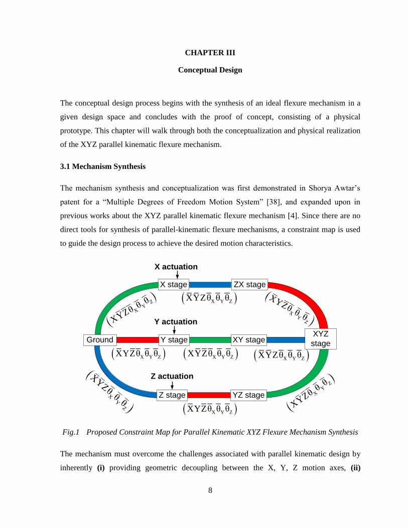
The mechanism synthesis and conceptualization was first demonstrated in Shorya Awtar’s

patent for a “Multiple Degrees of Freedom Motion System” [38], and expanded upon in

previous works about the XYZ parallel kinematic flexure mechanism [4]. Since there are no

direct tools for synthesis of parallel-kinematic flexure mechanisms, a constraint map is used

to guide the design process to achieve the desired motion characteristics.

X actuation

Y actuation

Z actuation

XY

Z

XYZθθθ

X Y ZXYZθ θ θ

X Y ZXYZθ θ θ

Ground

X stage ZX stage

Z stage YZ stage

XY stageY stageXYZ

stage

X Y ZXYZθ θ θ

X

YZ

XYZθθθ

X Y ZXYZθ θ θ

XY

Z

XY

Zθθθ

X Y ZXYZθ θ θ

XY

Z

XYZθθθ

Fig.1 Proposed Constraint Map for Parallel Kinematic XYZ Flexure Mechanism Synthesis

The mechanism must overcome the challenges associated with parallel kinematic design by

inherently (i) providing geometric decoupling between the X, Y, Z motion axes, (ii)

9

constraining motion along the three rotational directions, and (iii) providing

actuator/generator integration along each translational direction. This constraint map serves

as the basis for the synthesis of a novel, compact, parallel-kinematic XYZ flexure mechanism

design that embodies the above desired attributes.

The proposed constraint map shown in Fig.1 consists of two elements: blocks for the rigid

stages and colored connectors for the constraint elements. The rigid stages are labeled

according to the axes along which they are designed to move, i.e. Ground, X stage, Y stage,

Z stage, XY stage, YZ stage, ZX stage, and XYZ stage. The constraint elements are

classified by color, green, blue, and red, according to the axes along which they guide

motion. In addition, the symbols within the parentheses represent the potential three

translational and three rotational degrees of freedom (DoF) between any two of the rigid

stages. Letters without bars represent DoF directions, and letters with bars represent degree

of constraint (DoC) directions. For example, the green elements, denoted by X Y Z(XYZθ θ θ ) ,

constrain motion to the X direction only; the red elements, denoted by X Y Z(XYZθ θ θ ) , constrain

motion to the Y direction only; and the blue elements, denoted by X Y Z(XYZθ θ θ ) , constrain

motion to the Z direction only. In the subsequent paragraphs, I describe how such mobility

and constraint characteristics are achieved.

For a three DoF parallel-kinematic mechanism, there must be three parallel connecting paths

between Ground and the XYZ stage, one each for the X, Y, and Z directions. Each path

should have the following characteristics:

i. An actuation stage should be constrained to move in one translational direction only.

ii. Translational motion of this actuation stage should be entirely transmitted to the XYZ

Stage, while keeping the XYZ stage free to move in the other two directions.

iii. Rotational motions of the XYZ Stage should be constrained.

Thus, the X stage connects to Ground via a X Y Z(XYZθ θ θ )constraint that allows an X actuator to

be integrated at this location. To transmit the resulting X translation of the X stage to the

XYZ stage, while permitting relative Y and Z translations, these two stages connect through

a X Y Z(XYZθ θ θ ) constraint. In other words, the connection between the X and XYZ stages

10

should allow only Y and Z DoF, constraining all others. This is accomplished by connecting

a X Y Z(XYZθ θ θ ) constraint and a X Y Z(XYZθ θ θ ) constraint in series, as shown in Fig.1.

The Y and Z direction actuation paths follow the same rationale to complete the constraint

map. This design achieves geometric decoupling by providing actuation in one direction,

without affecting the other two directions. The resulting constraint map generates flexure

mechanism topologies that provide large, unconstrained translations in the X, Y, and Z

directions, as well as actuator isolation between the three translational directions, while

restricting all rotations.

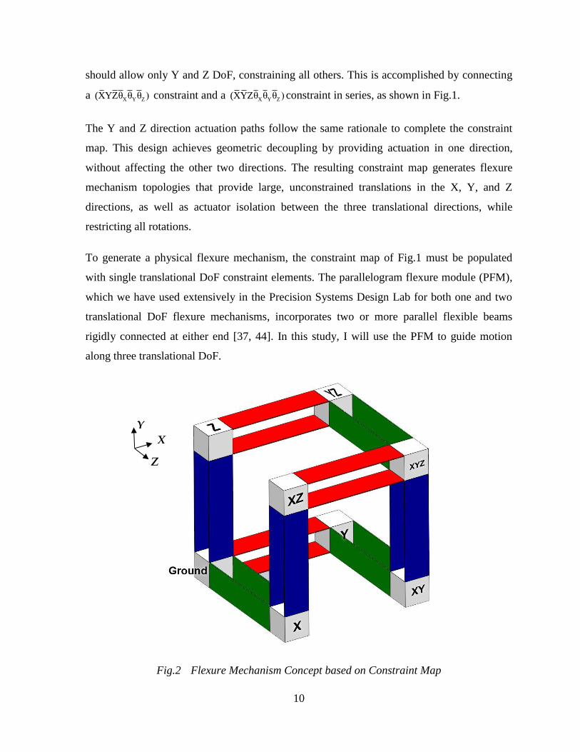
To generate a physical flexure mechanism, the constraint map of Fig.1 must be populated

with single translational DoF constraint elements. The parallelogram flexure module (PFM),

which we have used extensively in the Precision Systems Design Lab for both one and two

translational DoF flexure mechanisms, incorporates two or more parallel flexible beams

rigidly connected at either end [37, 44]. In this study, I will use the PFM to guide motion

along three translational DoF.

Fig.2 Flexure Mechanism Concept based on Constraint Map

X

Y

Z

11

The flexure mechanism produced by populating the above constraint map with PFMs is

shown in Fig.2. The white cubes representing the rigid stages are connected by the red,

green, and blue PFMs, according to the constraint map in Fig.1. The green PFMs deform

primarily in the X direction and remain stiff in all other directions; the red PFMs deform

primarily in the Y direction and remain stiff in all other directions; and, the blue PFMs

deform primarily in the Z direction and remain stiff in all other directions.

It is important to note that neither the constraint map in Fig.1 nor the physical realization in

Fig.2 follow the principles of “exact constraint” design [20]. For example, the rigid stages are

over-constrained to reduce potential rotations. This concept may be further augmented by

incorporating additional PFMs that serve as non-conflicting constraint elements to produce

the highly symmetric, cubic flexure mechanism shown in Fig.3. Again, the enhanced

symmetry resulting from this intentional over-constraint of the rigid stages reduces rotations

and cross-axis errors, while maintaining geometric decoupling and actuator isolation (See

Error! Reference source not found.). The distributed compliance of the PFMs enables

elastic averaging” [23], resulting in a design that is more tolerant to manufacturing and

assembly errors in spite of the over-constraint.

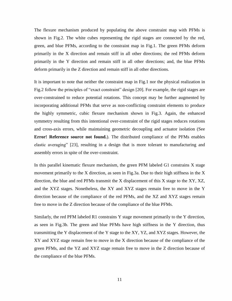
In this parallel kinematic flexure mechanism, the green PFM labeled G1 constrains X stage

movement primarily to the X direction, as seen in Fig.3a. Due to their high stiffness in the X

direction, the blue and red PFMs transmit the X displacement of this X stage to the XY, XZ,

and the XYZ stages. Nonetheless, the XY and XYZ stages remain free to move in the Y

direction because of the compliance of the red PFMs, and the XZ and XYZ stages remain

free to move in the Z direction because of the compliance of the blue PFMs.

Similarly, the red PFM labeled R1 constrains Y stage movement primarily to the Y direction,

as seen in Fig.3b. The green and blue PFMs have high stiffness in the Y direction, thus

transmitting the Y displacement of the Y stage to the XY, YZ, and XYZ stages. However, the

XY and XYZ stage remain free to move in the X direction because of the compliance of the

green PFMs, and the YZ and XYZ stage remain free to move in the Z direction because of

the compliance of the blue PFMs.

12

Finally, the blue PFM labeled B1

constrains Z stage movement

primarily to the Z direction, as seen in

Fig.3c. The green and red PFMs have

high stiffness in the Z direction, thus

transmitting the Z displacement of the

Z stage to the YZ, XZ, and XYZ

stages. However, the XZ and XYZ

stage remain free to move the X

direction because of the compliance of

the green PFMs, and the YZ and XYZ

stage remain free to move in the Y

direction because of the compliance of

the red PFMs.

In effect, the proposed parallel-

kinematic flexure design behaves like

a mechanical summation device – the

X motion of the X stage, the Y motion

of the Y stage, and the Z motion of the

Z stage combine to produce the XYZ

stage output. In a multi-axis

nanopositioning system, the outputs of

large-stroke, fixed-axis, linear

actuators, mounted at the X, Y, and Z

stages, combine to produce motion in

three DoF at the XYZ stage.

Conversely, the flexure mechanism

also serves as a mechanical separator –

the X, Y, and Z motions of the XYZ

stage are mechanically separated into

Fig.3 Proposed Flexure Mechanism Design: A. X

motion only B. Y motion only, C. Z motion only

a.

b.

c.

X

Y

Z

X

Y

Z

X

Y

Z

13

an X motion only at the X stage, a Y motion only at the Y stage, and a Z motion only at the Z

stage. In the context of multi-axis energy harvesting, large-stroke, fixed-axis, linear

generators, mounted at the X, Y, and Z stages, capture energy from a proof mass vibrating in

three DoF on the XYZ stage.

The constraint map of Fig.1 can also be populated using other single translational DoF

flexure modules, such as the multi-beam parallelogram and the double parallelogram. This

would result in different XYZ flexure mechanism embodiments, while containing the same

geometric decoupling and actuator isolation behavior as seen above. More detailed motion

performance such as error motions, stiffness variations, and dynamic behavior would

obviously be different for each. In fact, if the constraint elements were ideal, i.e. zero

stiffness and infinite motion in their DoF direction, and infinite stiffness and zero motions in

their constrained directions, the resulting XYZ flexure mechanism would also be ideal – zero

stiffness in the X, Y, and Z directions, zero parasitic rotations of all the stages, perfect

decoupling between the motion axes, perfect actuator isolation, zero lost motion between the

point of actuation and the main motion stage.

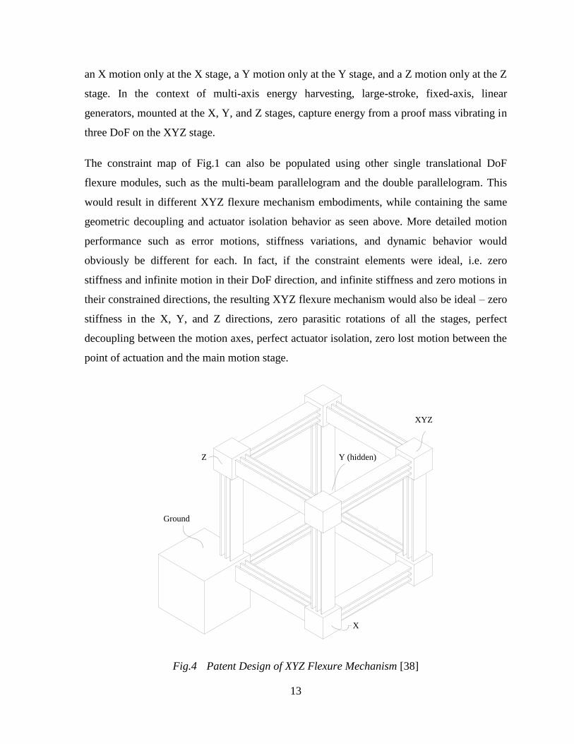
X

XYZ

Z

Ground

Y (hidden)

Fig.4 Patent Design of XYZ Flexure Mechanism [38]

14

However, in reality, elasticity of the flexure material inherently produces small, but finite,

stiffness in the DoF direction, and small, but finite, compliance in the constrained directions

[36]. This gives rise to small, but finite, deviations from the ideal motion behavior in any

XYZ flexure mechanism resulting from the above constraint map.

Therefore, validation of the conceptual design requires a physical model. I designed two

prototypes in CAD based on Shorya Awtar’s patented design shown in Fig.4 [38], and

subsequently fabricated and assembled them for the proof-of-concept.

Unlike planar flexure mechanisms [37], the complex geometry of the XYZ flexure

mechanism precludes monolithic fabrication. Therefore, the performance of the device relies

heavily on the manufacturing and assembly techniques used. Minimizing the number of

unique parts helps to ensure accurate and repeatable fabrication.

3.2 First Prototype

Although the design constraints and manufacturing principles were met, the first design was

not adequately analyzed for structural performance. The resulting prototype could flex in its

DoF directions, but buckled under its own weight. Therefore, it was inadequate for proving

the macro-scale performance characteristics of the concept design. The following presents a

detailed design and manufacturing process of the first prototype, and discusses the lessons

learned going into the next design.

The proof-of-concept design process consists of three important steps: choosing the material

and dimensions of the flexible constraint elements, referred to as beam flexures; conceiving a

method of mounting the beam flexures to rigid end plates, creating the PFMs; and

determining how to assemble and join all of the PFMs, creating the XYZ flexure mechanism.

As a proof-of-concept, the detailed motion performance characteristics were not as important

as the macro-scale validation of the motion range and geometric decoupling between the

input axes. Therefore, the primary focus was on mounting and assembling the PFMs, with

little emphasis on analyzing bearing performance.

15

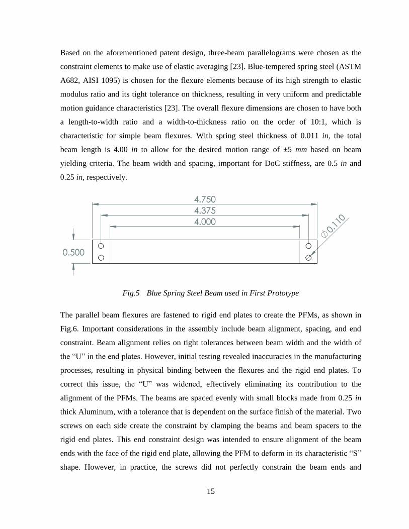
Based on the aforementioned patent design, three-beam parallelograms were chosen as the

constraint elements to make use of elastic averaging [23]. Blue-tempered spring steel (ASTM

A682, AISI 1095) is chosen for the flexure elements because of its high strength to elastic

modulus ratio and its tight tolerance on thickness, resulting in very uniform and predictable

motion guidance characteristics [23]. The overall flexure dimensions are chosen to have both

a length-to-width ratio and a width-to-thickness ratio on the order of 10:1, which is

characteristic for simple beam flexures. With spring steel thickness of 0.011 in, the total

beam length is 4.00 in to allow for the desired motion range of ±5 mm based on beam

yielding criteria. The beam width and spacing, important for DoC stiffness, are 0.5 in and

0.25 in, respectively.

Fig.5 Blue Spring Steel Beam used in First Prototype

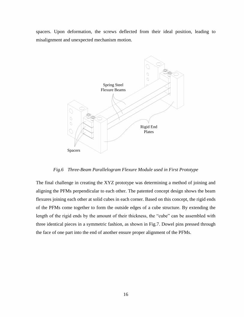
The parallel beam flexures are fastened to rigid end plates to create the PFMs, as shown in

Fig.6. Important considerations in the assembly include beam alignment, spacing, and end

constraint. Beam alignment relies on tight tolerances between beam width and the width of

the “U” in the end plates. However, initial testing revealed inaccuracies in the manufacturing

processes, resulting in physical binding between the flexures and the rigid end plates. To

correct this issue, the “U” was widened, effectively eliminating its contribution to the

alignment of the PFMs. The beams are spaced evenly with small blocks made from 0.25 in

thick Aluminum, with a tolerance that is dependent on the surface finish of the material. Two

screws on each side create the constraint by clamping the beams and beam spacers to the

rigid end plates. This end constraint design was intended to ensure alignment of the beam

ends with the face of the rigid end plate, allowing the PFM to deform in its characteristic “S”

shape. However, in practice, the screws did not perfectly constrain the beam ends and

16

spacers. Upon deformation, the screws deflected from their ideal position, leading to

misalignment and unexpected mechanism motion.

Spring Steel

Flexure Beams

Rigid End

Plates

Spacers

Fig.6 Three-Beam Parallelogram Flexure Module used in First Prototype

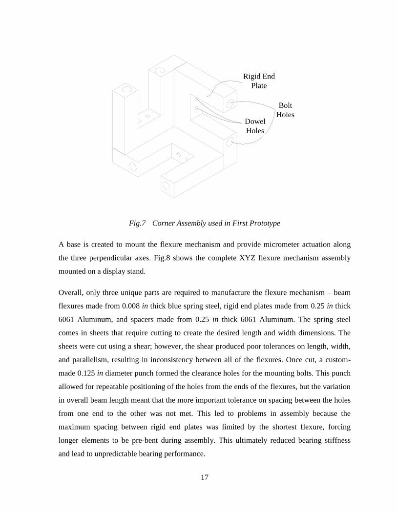
The final challenge in creating the XYZ prototype was determining a method of joining and

aligning the PFMs perpendicular to each other. The patented concept design shows the beam

flexures joining each other at solid cubes in each corner. Based on this concept, the rigid ends

of the PFMs come together to form the outside edges of a cube structure. By extending the

length of the rigid ends by the amount of their thickness, the “cube” can be assembled with

three identical pieces in a symmetric fashion, as shown in Fig.7. Dowel pins pressed through

the face of one part into the end of another ensure proper alignment of the PFMs.

17

Rigid End

Plate

Bolt

HolesDowel

Holes

Fig.7 Corner Assembly used in First Prototype

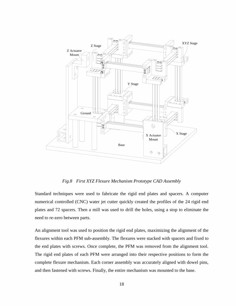
A base is created to mount the flexure mechanism and provide micrometer actuation along

the three perpendicular axes. Fig.8 shows the complete XYZ flexure mechanism assembly

mounted on a display stand.

Overall, only three unique parts are required to manufacture the flexure mechanism – beam

flexures made from 0.008 in thick blue spring steel, rigid end plates made from 0.25 in thick

6061 Aluminum, and spacers made from 0.25 in thick 6061 Aluminum. The spring steel

comes in sheets that require cutting to create the desired length and width dimensions. The

sheets were cut using a shear; however, the shear produced poor tolerances on length, width,

and parallelism, resulting in inconsistency between all of the flexures. Once cut, a custom-

made 0.125 in diameter punch formed the clearance holes for the mounting bolts. This punch

allowed for repeatable positioning of the holes from the ends of the flexures, but the variation

in overall beam length meant that the more important tolerance on spacing between the holes

from one end to the other was not met. This led to problems in assembly because the

maximum spacing between rigid end plates was limited by the shortest flexure, forcing

longer elements to be pre-bent during assembly. This ultimately reduced bearing stiffness

and lead to unpredictable bearing performance.

18

Ground

X Actuator

Mount

Z Actuator

Mount

Z Stage

X Stage

Y Stage

XYZ Stage

Base

Fig.8 First XYZ Flexure Mechanism Prototype CAD Assembly

Standard techniques were used to fabricate the rigid end plates and spacers. A computer

numerical controlled (CNC) water jet cutter quickly created the profiles of the 24 rigid end

plates and 72 spacers. Then a mill was used to drill the holes, using a stop to eliminate the

need to re-zero between parts.

An alignment tool was used to position the rigid end plates, maximizing the alignment of the

flexures within each PFM sub-assembly. The flexures were stacked with spacers and fixed to

the end plates with screws. Once complete, the PFM was removed from the alignment tool.

The rigid end plates of each PFM were arranged into their respective positions to form the

complete flexure mechanism. Each corner assembly was accurately aligned with dowel pins,

and then fastened with screws. Finally, the entire mechanism was mounted to the base.

19

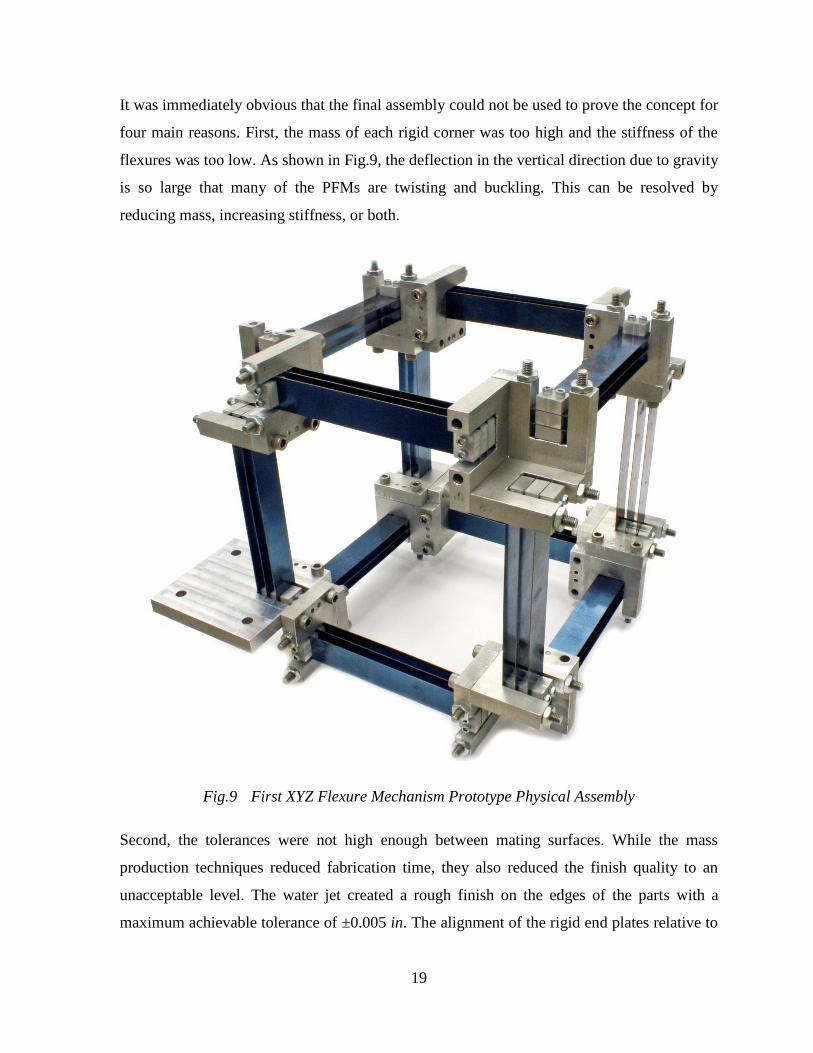
It was immediately obvious that the final assembly could not be used to prove the concept for

four main reasons. First, the mass of each rigid corner was too high and the stiffness of the

flexures was too low. As shown in Fig.9, the deflection in the vertical direction due to gravity

is so large that many of the PFMs are twisting and buckling. This can be resolved by

reducing mass, increasing stiffness, or both.

Fig.9 First XYZ Flexure Mechanism Prototype Physical Assembly

Second, the tolerances were not high enough between mating surfaces. While the mass

production techniques reduced fabrication time, they also reduced the finish quality to an

unacceptable level. The water jet created a rough finish on the edges of the parts with a

maximum achievable tolerance of ±0.005 in. The alignment of the rigid end plates relative to

20

one another relies on the quality of the mating surfaces, which includes the rough edges

created by the water jet. This resulted in a less-than-optimal assembly of the corners.

Additionally, the poor surface finish exaggerated the over constraint caused by the dowel

pins, making assembly with all of the dowel pins impossible. This can be resolved by finish

milling the surfaces with a greater tolerance, and reconsidering the alignment method to

eliminate the potential for over constraint.

Third, the dimensional and alignment tolerances of the beam flexures were very low. As

noted previously, the shearing process could not produce a consistent final product. The

shear tends to lift the material next to the shearing point which causes a variance in width

along the length of each piece as much as ±0.05 in. This is greater than the intermediate stage

“U” width tolerance of ±0.01 in. Also, the bolts used to clamp the flexures and spacers were

used to constrain the assembly with respect to the stage, but axial forces could bend the bolts

slightly. To remedy these problems, the flexures could be cut on the water jet with a length

tolerance of ±0.005 in, which is an order of magnitude better than on the shear. A better

method of constraint is required to ensure proper alignment of the flexures within the PFMs.

Finally, the sheer quantity of parts becomes a large tolerance stack-up. The tolerances of each

individual part in series are added, resulting in an unexpectedly large tolerance between the

Ground and the XYZ stage. Reducing the total number of parts not only improves the overall

tolerance stack-up; it also reduces the number of mating surfaces that require alignment

features.

3.3 Second Prototype

The main goal of validating the qualitative performance of the concept design was not

accomplished in the first prototype because it buckled under its own weight. Therefore, the

next design iteration focused on reducing weight, increasing stiffness, and analyzing the

structural performance of the flexures under load to ensure successful completion of the

proof-of-concept. To reduce weight, the material used for the rigid ends was changed from

Aluminum to plastic. Thicker blue spring steel, 0.011 in as opposed to 0.008 in, was chosen

for the flexures because stiffness increases by thickness cubed. Additionally, I increased

beam width from 0.5 in to 1.0 in, and the spacing between the outermost beams from 0.5 in

21

to 1.0 in. Increasing these dimensions subsequently increases the rotational stiffness about

the axis along the beam’s length to help mitigate the buckling seen in the previous design.

Preliminary analysis of the effect of gravity on the vertical displacement of the revised

bearing predicted only a 0.5 mm drop from its undeformed position; a great improvement

over the approximately 10 mm drop seen on the first design.

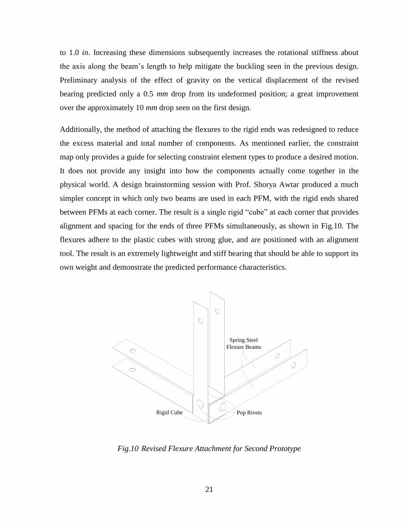
Additionally, the method of attaching the flexures to the rigid ends was redesigned to reduce

the excess material and total number of components. As mentioned earlier, the constraint

map only provides a guide for selecting constraint element types to produce a desired motion.

It does not provide any insight into how the components actually come together in the

physical world. A design brainstorming session with Prof. Shorya Awtar produced a much

simpler concept in which only two beams are used in each PFM, with the rigid ends shared

between PFMs at each corner. The result is a single rigid “cube” at each corner that provides

alignment and spacing for the ends of three PFMs simultaneously, as shown in Fig.10. The

flexures adhere to the plastic cubes with strong glue, and are positioned with an alignment

tool. The result is an extremely lightweight and stiff bearing that should be able to support its

own weight and demonstrate the predicted performance characteristics.

Spring Steel

Flexure Beams

Pop RivetsRigid Cube

Fig.10 Revised Flexure Attachment for Second Prototype

22

The much simplified, second prototype has only two unique components – beam flexures

made of blue spring steel and rigid cubes made of plastic. The flexures are now cut on the

water jet cutter to produce a tolerance of 0.001 in, which is an order of magnitude better than

those produced using a sheet metal shear. The tolerances are still not adequate for use in a

nanopositioner because misalignment, even on the order of 0.001 in, can cause greatly

varying stiffnesses. However, the tolerances are acceptable for proving the concept. The

plastic cubes are cut from a plate, and finish milled to ensure proper dimensioning and

flatness. Much slower feed rates must be used when milling or drilling plastic, as heat

generated from the cutting process can melt and distort the finish of the material.

During assembly, several different types of glues were tested for adherence and strength.

First, ordinary super glue was applied between the spring steel and plastic. Super glue is

extremely fast setting, and does not allow sufficient time for proper placement of the flexures

with respect to the rigid cube in the alignment tool. Additionally, super glue does not have

the peel strength required for the amount of expected bearing deflection. Next, Loctite 1

Minute Epoxy was tried with similar failure. While the setting time is slow enough to allow

proper alignment, the peel strength is also inadequate. Finally, a special-ordered industrial

strength epoxy, Chemical Concepts K45-S-14ML, which is designed for metal and acrylic,

was tested. This epoxy produced very strong fumes, and was difficult to work with because it

generated a significant amount of heat. While this last epoxy was the strongest glue tested, it

still failed to meet the peel strength requirements. After all testing was completed, it was

discovered that the plastic cubes were actually made from Nylon scrap from the lab, which

has very poor bonding properties. Materials such as low-density polyethylene or PVC would

have provided better adhesive properties, but instead of changing the cube material, a

mechanical constraint was added to ensure bonding between the components over repeated

cycling of the flexure mechanism.

23

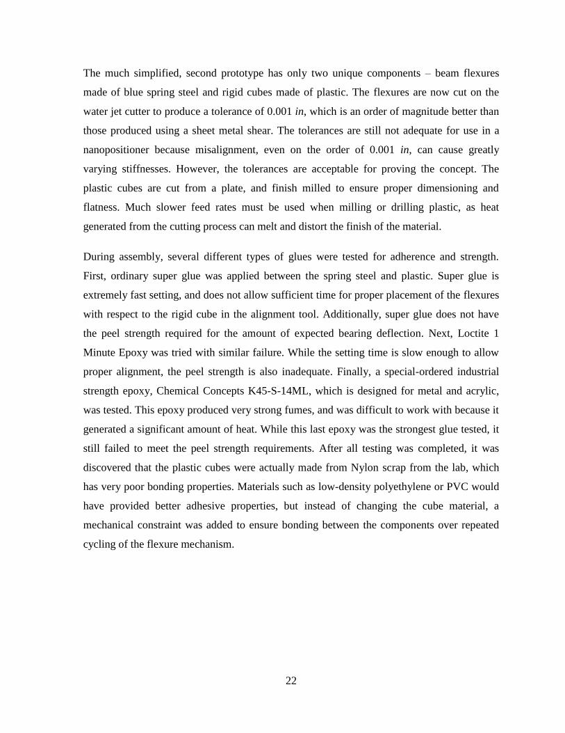
Fig.11 Rigid Cube with Holes for Rivets

The design was modified to include a mechanical constraint element, ensuring a rigid

constraint at the ends of each PFM. 1/8 in diameter aluminum pop rivets were chosen

because they provide a very light weight, yet strong attachment. The cubes were drilled with

off-center holes so that three perpendicular rivets could be installed without interference.

Fig.11 shows a CAD model of a cube with hidden lines visible to highlight the placement of

the holes. Clearance holes were punched on the ends of the flexures to allow for slight

manufacturing variation. Even if the cube material had been properly chosen for the glue, a

mechanical constraint guarantees a much longer life for the stress cycles imparted through

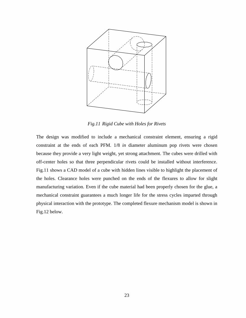
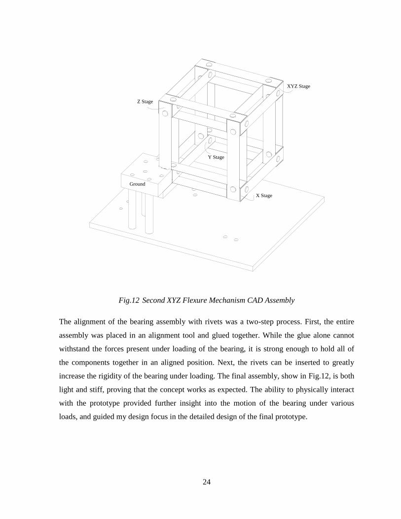
physical interaction with the prototype. The completed flexure mechanism model is shown in

Fig.12 below.

24

Ground

X Stage

Z Stage

XYZ Stage

Y Stage

Fig.12 Second XYZ Flexure Mechanism CAD Assembly

The alignment of the bearing assembly with rivets was a two-step process. First, the entire

assembly was placed in an alignment tool and glued together. While the glue alone cannot

withstand the forces present under loading of the bearing, it is strong enough to hold all of

the components together in an aligned position. Next, the rivets can be inserted to greatly

increase the rigidity of the bearing under loading. The final assembly, show in Fig.12, is both

light and stiff, proving that the concept works as expected. The ability to physically interact

with the prototype provided further insight into the motion of the bearing under various

loads, and guided my design focus in the detailed design of the final prototype.

25

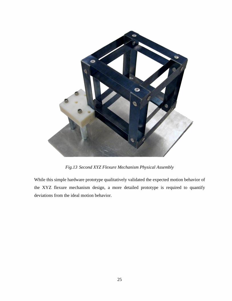
Fig.13 Second XYZ Flexure Mechanism Physical Assembly

While this simple hardware prototype qualitatively validated the expected motion behavior of

the XYZ flexure mechanism design, a more detailed prototype is required to quantify

deviations from the ideal motion behavior.

26

CHAPTER IV

Detailed Design

This chapter covers the detailed design of the XYZ parallel kinematic flexure mechanism

concept presented in the previous chapter. The design process covers the selection of the

flexure material and dimensions based on desired static motion performance and design

constraints, prediction of the static motion performance through non-linear FEA, and

physical CAD modeling of the entire mechanism assembly for subsequent fabrication and

validation.

4.1 Flexure Dimensioning and Material Selection

The overall size, detailed dimensions, and material selection for the flexure mechanism are

determined using a static failure (i.e., material yielding) criterion. For a rectangular cantilever

beam with a concentrated load at one end, the maximum stress is given by:

2

3 E T

2 L

where Δ is the beam end deflection, E is the Young’s modulus, T is the beam thickness, and L

is the beam length. Given the geometry and constraint pattern of the proposed design, it is

evident that the constituent beam flexures deform predominantly in an S-shape. For this

deformation, the maximum allowable end-deflection of a beam before the onset of yielding is

given by:

2

yS1 1 L

3 E T

where η is the factor of safety, Sy is the yield strength, E is the Young’s modulus, T is the

beam thickness, and L is the beam length, as shown in Fig.14.

27

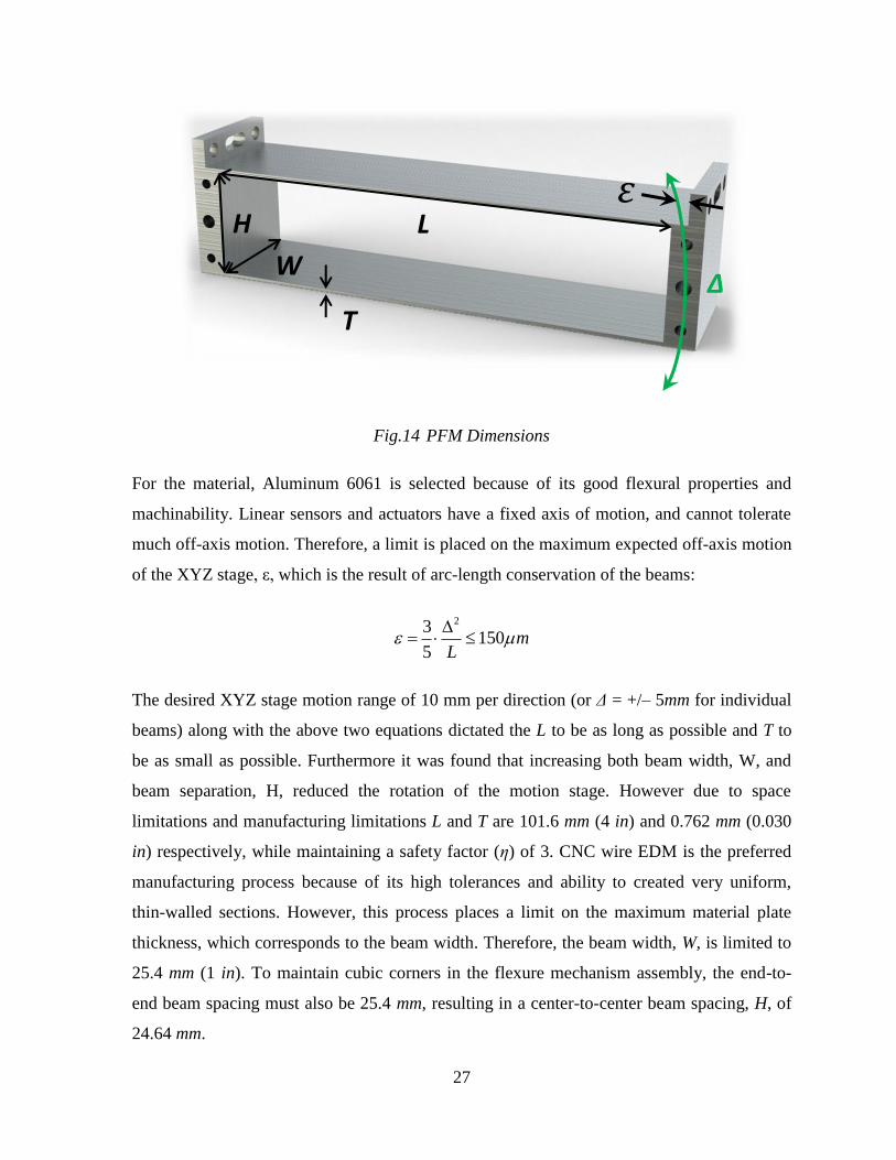
Fig.14 PFM Dimensions

For the material, Aluminum 6061 is selected because of its good flexural properties and

machinability. Linear sensors and actuators have a fixed axis of motion, and cannot tolerate

much off-axis motion. Therefore, a limit is placed on the maximum expected off-axis motion

of the XYZ stage, ε, which is the result of arc-length conservation of the beams:

23150

5m

L

The desired XYZ stage motion range of 10 mm per direction (or Δ = +/– 5mm for individual

beams) along with the above two equations dictated the L to be as long as possible and T to

be as small as possible. Furthermore it was found that increasing both beam width, W, and

beam separation, H, reduced the rotation of the motion stage. However due to space

limitations and manufacturing limitations L and T are 101.6 mm (4 in) and 0.762 mm (0.030

in) respectively, while maintaining a safety factor (η) of 3. CNC wire EDM is the preferred

manufacturing process because of its high tolerances and ability to created very uniform,

thin-walled sections. However, this process places a limit on the maximum material plate

thickness, which corresponds to the beam width. Therefore, the beam width, W, is limited to

25.4 mm (1 in). To maintain cubic corners in the flexure mechanism assembly, the end-to-

end beam spacing must also be 25.4 mm, resulting in a center-to-center beam spacing, H, of

24.64 mm.

H

W

L

T

ε

Δ

28

4.2 Predicted Motion Performance

Predicting the detailed motion performance of large range flexure mechanisms requires a

non-linear force-displacement analysis, as shown previously [19, 36]. Ideally, a closed-form,

non-linear analysis is preferable since it offers quantitative and parametric insight into the

relation between the mechanism’s geometry and its motion performance. However, such an

analysis entails considerable mathematical complexity and is the subject of our research

group’s ongoing and future work. Instead, to expediently obtain some early validation and

assessment of the proposed design, I conducted non-linear finite elements analysis (FEA)

using ANSYS.

X

Y

Z

SHELL 181

Mesh

MPC184 Rigid

Elements

Ground

DoF

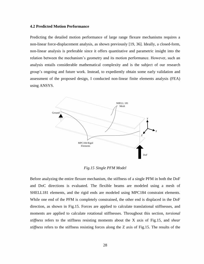
Fig.15 Single PFM Model

Before analyzing the entire flexure mechanism, the stiffness of a single PFM in both the DoF

and DoC directions is evaluated. The flexible beams are modeled using a mesh of

SHELL181 elements, and the rigid ends are modeled using MPC184 constraint elements.

While one end of the PFM is completely constrained, the other end is displaced in the DoF

direction, as shown in Fig.15. Forces are applied to calculate translational stiffnesses, and

moments are applied to calculate rotational stiffnesses. Throughout this section, torsional

stiffness refers to the stiffness resisting moments about the X axis of Fig.15, and shear

stiffness refers to the stiffness resisting forces along the Z axis of Fig.15. The results of the

29

single PFM stiffness analysis help explain the more complex nonlinear behavior of the

overall XYZ flexure mechanism shown later.

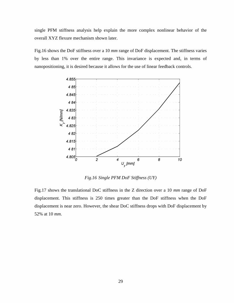
Fig.16 shows the DoF stiffness over a 10 mm range of DoF displacement. The stiffness varies

by less than 1% over the entire range. This invariance is expected and, in terms of

nanopositioning, it is desired because it allows for the use of linear feedback controls.

Fig.16 Single PFM DoF Stiffness (UY)

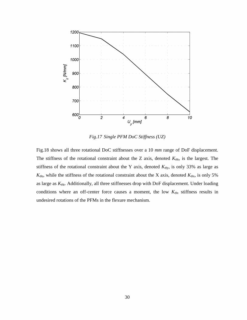
Fig.17 shows the translational DoC stiffness in the Z direction over a 10 mm range of DoF

displacement. This stiffness is 250 times greater than the DoF stiffness when the DoF

displacement is near zero. However, the shear DoC stiffness drops with DoF displacement by

52% at 10 mm.

30

Fig.17 Single PFM DoC Stiffness (UZ)

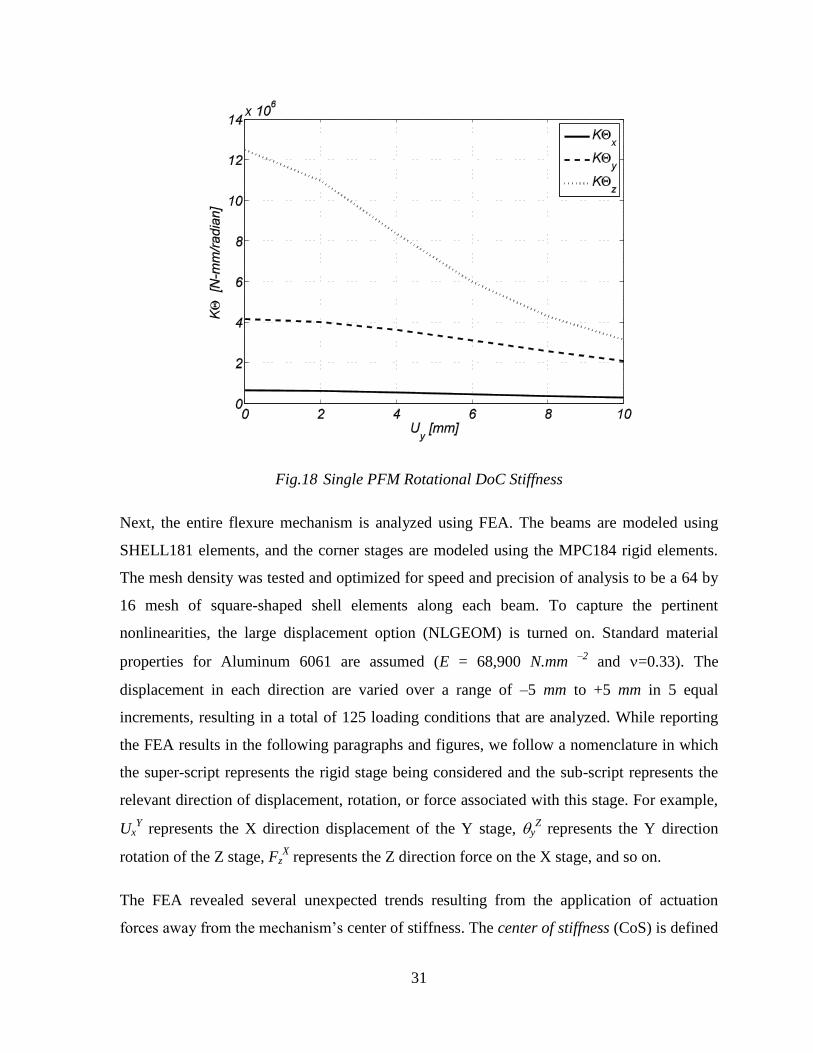
Fig.18 shows all three rotational DoC stiffnesses over a 10 mm range of DoF displacement.

The stiffness of the rotational constraint about the Z axis, denoted KΘz, is the largest. The

stiffness of the rotational constraint about the Y axis, denoted KΘy, is only 33% as large as

KΘz, while the stiffness of the rotational constraint about the X axis, denoted KΘx, is only 5%

as large as KΘz. Additionally, all three stiffnesses drop with DoF displacement. Under loading

conditions where an off-center force causes a moment, the low KΘx stiffness results in

undesired rotations of the PFMs in the flexure mechanism.

31

Fig.18 Single PFM Rotational DoC Stiffness

Next, the entire flexure mechanism is analyzed using FEA. The beams are modeled using

SHELL181 elements, and the corner stages are modeled using the MPC184 rigid elements.

The mesh density was tested and optimized for speed and precision of analysis to be a 64 by

16 mesh of square-shaped shell elements along each beam. To capture the pertinent

nonlinearities, the large displacement option (NLGEOM) is turned on. Standard material

properties for Aluminum 6061 are assumed (E = 68,900 N.mm –2

and =0.33). The

displacement in each direction are varied over a range of ‒5 mm to +5 mm in 5 equal

increments, resulting in a total of 125 loading conditions that are analyzed. While reporting

the FEA results in the following paragraphs and figures, we follow a nomenclature in which

the super-script represents the rigid stage being considered and the sub-script represents the

relevant direction of displacement, rotation, or force associated with this stage. For example,

UxY represents the X direction displacement of the Y stage, y

Z represents the Y direction

rotation of the Z stage, FzX represents the Z direction force on the X stage, and so on.

The FEA revealed several unexpected trends resulting from the application of actuation

forces away from the mechanism’s center of stiffness. The center of stiffness (CoS) is defined

32

as the point on each plane perpendicular to the actuation axes at which an actuation force

applied through the actuation stage produces minimal rotations at the XYZ stage. Actuating

through the CoS is critical for bearing performance because parasitic rotations cannot be

actively controlled by the three linear actuators. The exact CoS for each actuation stage is

difficult to determine, and does not remain constant for all combinations of X, Y, and Z

actuations. However, an estimate of the CoS for each actuation direction can be determined

through minimizing the XYZ stage rotations in a static displacement FEA of the mechanism.

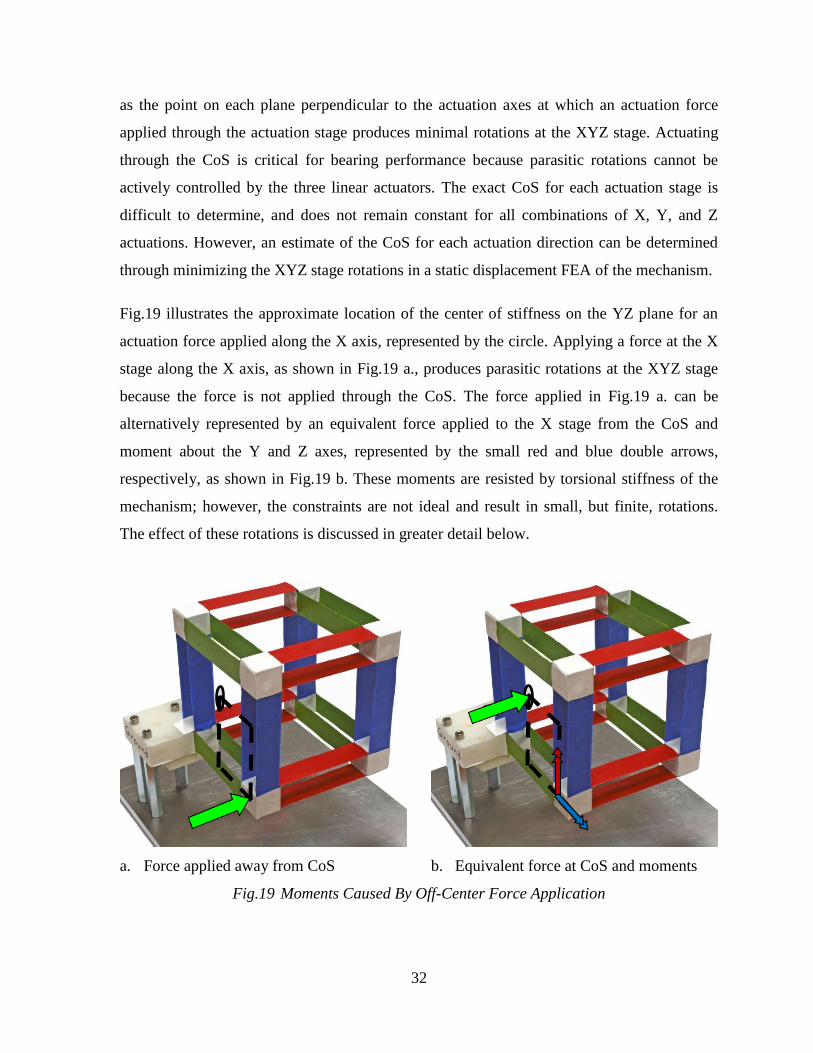
Fig.19 illustrates the approximate location of the center of stiffness on the YZ plane for an

actuation force applied along the X axis, represented by the circle. Applying a force at the X

stage along the X axis, as shown in Fig.19 a., produces parasitic rotations at the XYZ stage

because the force is not applied through the CoS. The force applied in Fig.19 a. can be

alternatively represented by an equivalent force applied to the X stage from the CoS and

moment about the Y and Z axes, represented by the small red and blue double arrows,

respectively, as shown in Fig.19 b. These moments are resisted by torsional stiffness of the

mechanism; however, the constraints are not ideal and result in small, but finite, rotations.

The effect of these rotations is discussed in greater detail below.

a. Force applied away from CoS b. Equivalent force at CoS and moments

Fig.19 Moments Caused By Off-Center Force Application

33

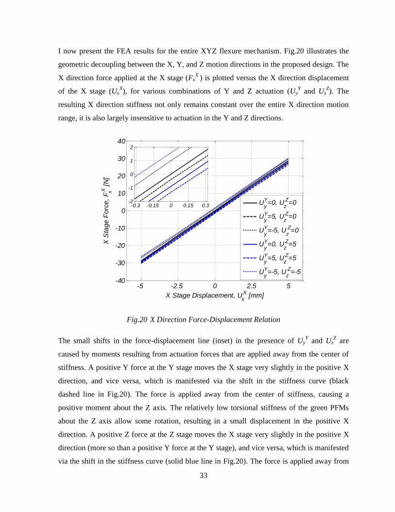
I now present the FEA results for the entire XYZ flexure mechanism. Fig.20 illustrates the

geometric decoupling between the X, Y, and Z motion directions in the proposed design. The

X direction force applied at the X stage (FxX

) is plotted versus the X direction displacement

of the X stage (UxX), for various combinations of Y and Z actuation (Uy

Y and Uz

Z). The

resulting X direction stiffness not only remains constant over the entire X direction motion

range, it is also largely insensitive to actuation in the Y and Z directions.

Fig.20 X Direction Force-Displacement Relation

The small shifts in the force-displacement line (inset) in the presence of UyY and Uz

Z are

caused by moments resulting from actuation forces that are applied away from the center of

stiffness. A positive Y force at the Y stage moves the X stage very slightly in the positive X

direction, and vice versa, which is manifested via the shift in the stiffness curve (black

dashed line in Fig.20). The force is applied away from the center of stiffness, causing a

positive moment about the Z axis. The relatively low torsional stiffness of the green PFMs

about the Z axis allow some rotation, resulting in a small displacement in the positive X

direction. A positive Z force at the Z stage moves the X stage very slightly in the positive X

direction (more so than a positive Y force at the Y stage), and vice versa, which is manifested

via the shift in the stiffness curve (solid blue line in Fig.20). The force is applied away from

-5 -2.5 0 2.5 5-40

-30

-20

-10

0

10

20

30

40

X Stage Displacement, Ux

X [mm]

X S

tag

e F

orc

e,

Fx X

[N

]

Uy

Y=0, U

z

Z=0

Uy

Y=5, U

z

Z=0

Uy

Y=-5, U

z

Z=0

Uy

Y=0, U

z

Z=5

Uy

Y=5, U

z

Z=5

Uy

Y=-5, U

z

Z=-5

-0.3 -0.15 0 0.15 0.3-2

-1

0

1

2

34

the center of stiffness, causing a positive moment about the Y axis. The relatively low

torsional stiffness of the blue PFMs about the Y axis allows some rotation, resulting in a

small displacement in the positive X direction.

Although not plotted here, the Y and Z direction stiffness also exhibit a similar behavior

because of the symmetric design. This validates the unique attribute of the proposed flexure

mechanism that its mobility in one direction is not influenced by motion in the other

directions. This decoupling allows large motions in each direction, unconstrained by the

geometry and limited only by material failure.

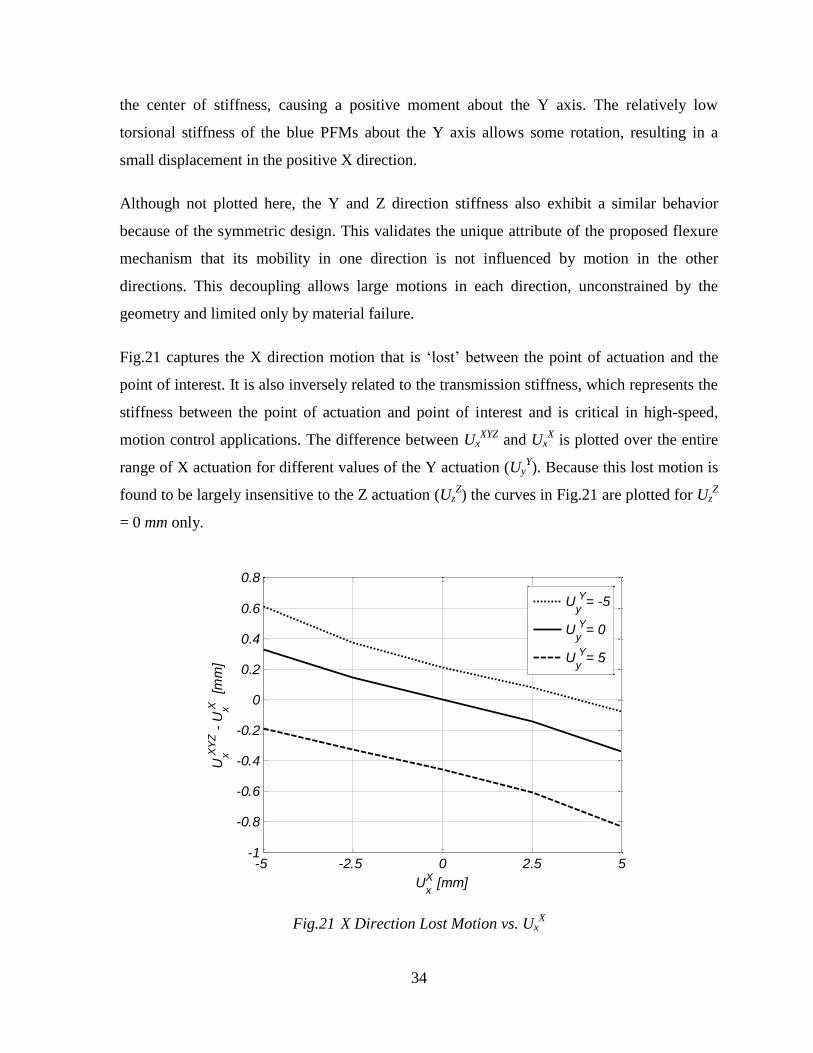
Fig.21 captures the X direction motion that is ‘lost’ between the point of actuation and the

point of interest. It is also inversely related to the transmission stiffness, which represents the

stiffness between the point of actuation and point of interest and is critical in high-speed,

motion control applications. The difference between UxXYZ

and UxX is plotted over the entire

range of X actuation for different values of the Y actuation (UyY). Because this lost motion is

found to be largely insensitive to the Z actuation (UzZ) the curves in Fig.21 are plotted for Uz

Z

= 0 mm only.

Fig.21 X Direction Lost Motion vs. UxX

-5 -2.5 0 2.5 5-1

-0.8

-0.6

-0.4

-0.2

0

0.2

0.4

0.6

0.8

Ux

X [mm]

Ux X

YZ -

Ux X

[m

m]

Uy

Y= -5

Uy

Y= 0

Uy

Y= 5

35

When UyY and Uz

Z actuation are zero, the lost motion varies nearly linearly with Ux

X. As

previously shown in Fig.20, the UxX varies linearly with Fx

X. Because the center of stiffness is

not varying much with UxX, the subsequent moment also varies linearly with Ux

X. The

relatively low torsional stiffness of the green PFMs about the Z axis allow a small amount of

rotation about the positive Z axis. Therefore, this rotation also varies linearly with UxX. The

blue PFMs remain nearly straight due to their relatively large shear stiffness, and the

resulting lost motion varies linearly with the sine of this angle. The rotation is small

(maximum 2.6 mrad), so the sine of the angle can be approximated as the angle alone.

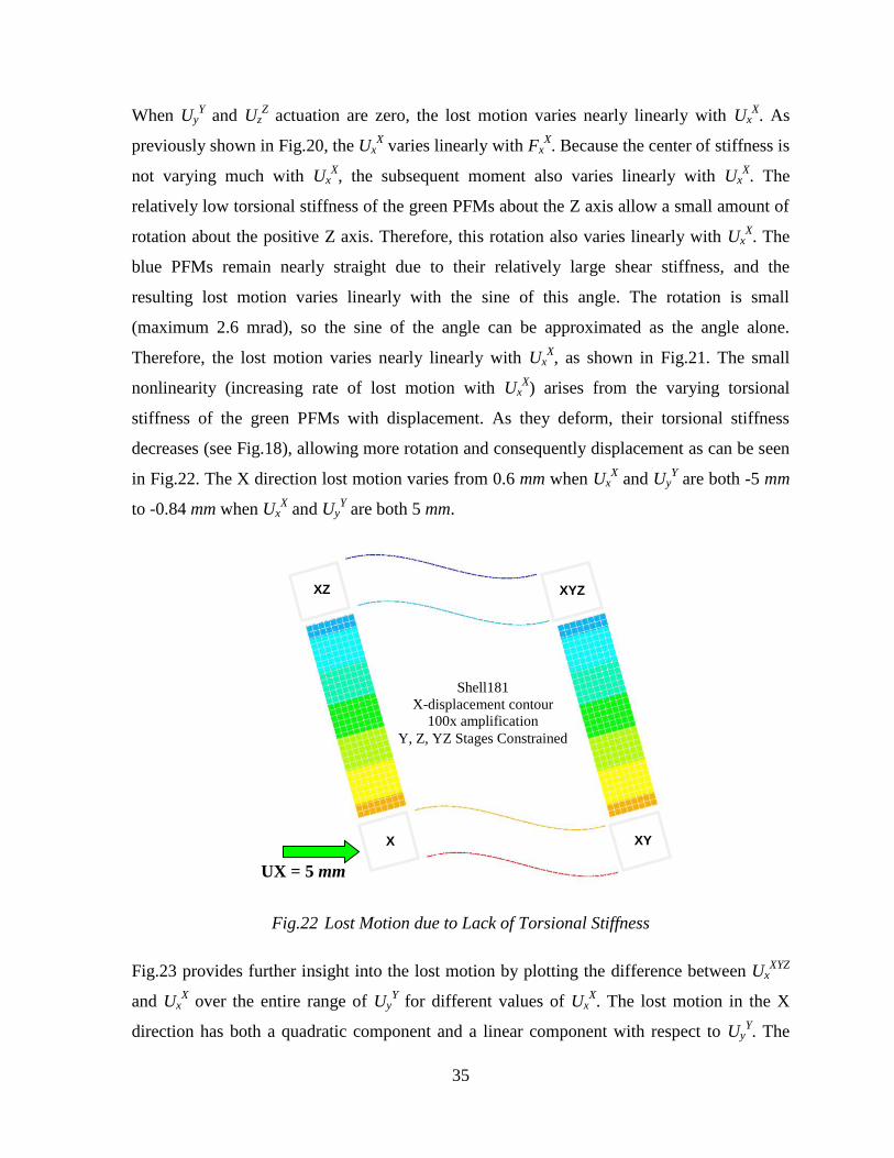
Therefore, the lost motion varies nearly linearly with UxX, as shown in Fig.21. The small

nonlinearity (increasing rate of lost motion with UxX) arises from the varying torsional

stiffness of the green PFMs with displacement. As they deform, their torsional stiffness

decreases (see Fig.18), allowing more rotation and consequently displacement as can be seen

in Fig.22. The X direction lost motion varies from 0.6 mm when UxX and Uy

Y are both -5 mm

to -0.84 mm when UxX and Uy

Y are both 5 mm.

Fig.22 Lost Motion due to Lack of Torsional Stiffness

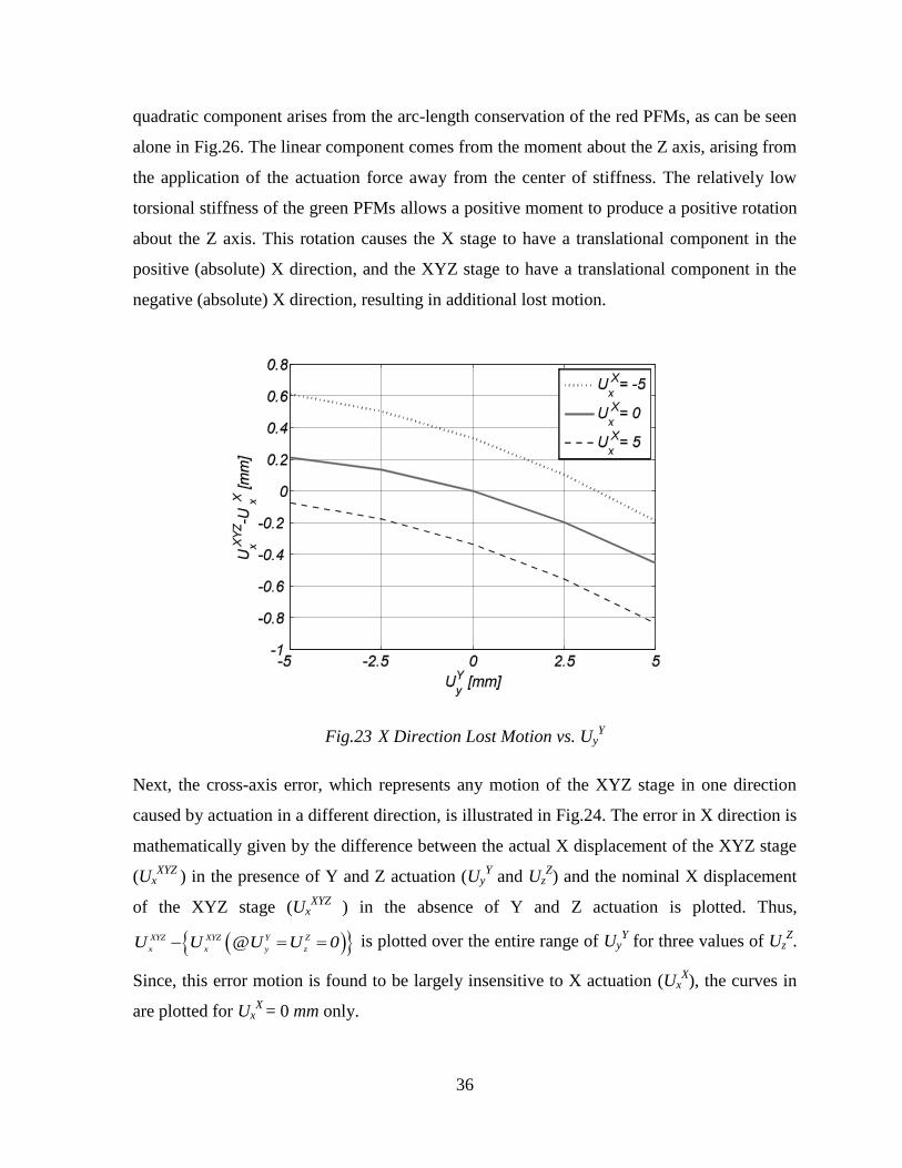
Fig.23 provides further insight into the lost motion by plotting the difference between UxXYZ

and UxX over the entire range of Uy

Y for different values of Ux

X. The lost motion in the X

direction has both a quadratic component and a linear component with respect to UyY. The

XZ XYZ

XY

UX = 5 mm

Shell181

X-displacement contour

100x amplification

Y, Z, YZ Stages Constrained

X

36

quadratic component arises from the arc-length conservation of the red PFMs, as can be seen

alone in Fig.26. The linear component comes from the moment about the Z axis, arising from

the application of the actuation force away from the center of stiffness. The relatively low

torsional stiffness of the green PFMs allows a positive moment to produce a positive rotation

about the Z axis. This rotation causes the X stage to have a translational component in the

positive (absolute) X direction, and the XYZ stage to have a translational component in the

negative (absolute) X direction, resulting in additional lost motion.

Fig.23 X Direction Lost Motion vs. UyY

Next, the cross-axis error, which represents any motion of the XYZ stage in one direction

caused by actuation in a different direction, is illustrated in Fig.24. The error in X direction is

mathematically given by the difference between the actual X displacement of the XYZ stage

(UxXYZ

) in the presence of Y and Z actuation (UyY and Uz

Z) and the nominal X displacement

of the XYZ stage (UxXYZ

) in the absence of Y and Z actuation is plotted. Thus,

@XYZ XYZ Y Z

x x y zU U U U 0 is plotted over the entire range of Uy

Y for three values of Uz

Z.

Since, this error motion is found to be largely insensitive to X actuation (UxX), the curves in

are plotted for UxX

= 0 mm only.

37

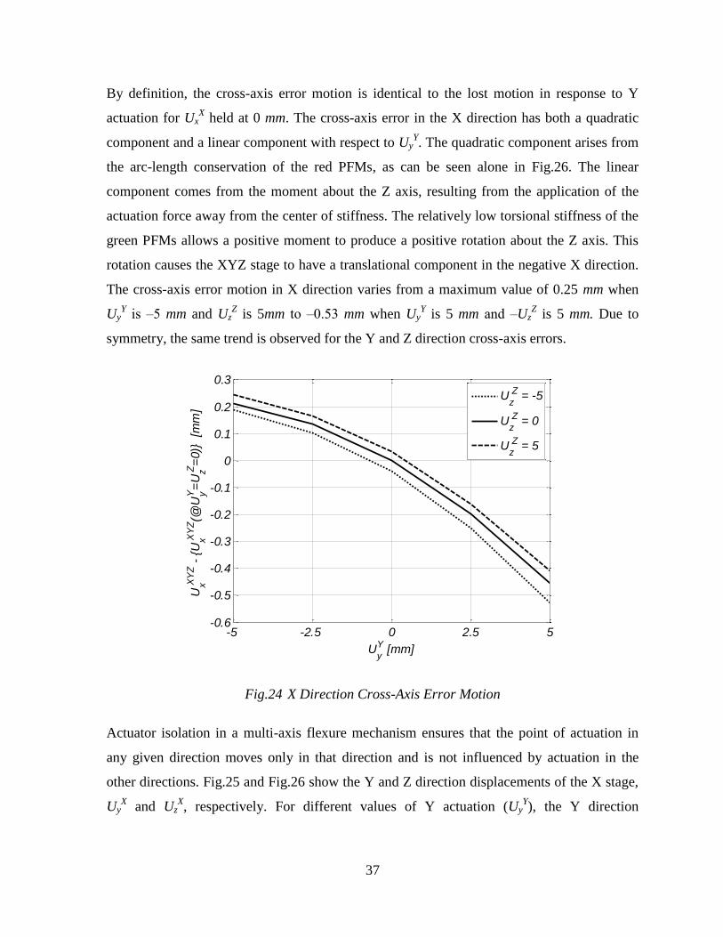
By definition, the cross-axis error motion is identical to the lost motion in response to Y

actuation for UxX held at 0 mm. The cross-axis error in the X direction has both a quadratic

component and a linear component with respect to UyY. The quadratic component arises from

the arc-length conservation of the red PFMs, as can be seen alone in Fig.26. The linear

component comes from the moment about the Z axis, resulting from the application of the

actuation force away from the center of stiffness. The relatively low torsional stiffness of the

green PFMs allows a positive moment to produce a positive rotation about the Z axis. This

rotation causes the XYZ stage to have a translational component in the negative X direction.

The cross-axis error motion in X direction varies from a maximum value of 0.25 mm when

UyY is ‒5 mm and Uz

Z is 5mm to ‒0.53 mm when Uy

Y is 5 mm and ‒Uz

Z is 5 mm. Due to

symmetry, the same trend is observed for the Y and Z direction cross-axis errors.

Fig.24 X Direction Cross-Axis Error Motion

Actuator isolation in a multi-axis flexure mechanism ensures that the point of actuation in

any given direction moves only in that direction and is not influenced by actuation in the

other directions. Fig.25 and Fig.26 show the Y and Z direction displacements of the X stage,

UyX and Uz

X, respectively. For different values of Y actuation (Uy

Y), the Y direction

-5 -2.5 0 2.5 5-0.6

-0.5

-0.4

-0.3

-0.2

-0.1

0

0.1

0.2

0.3

Uy

Y [mm]

Ux X

YZ -

{U

x XY

Z(@

UyY=

Uz Z

=0)}

[m

m]

Uz

Z = -5

Uz

Z = 0

Uz

Z = 5

38

displacement of the X stage (UyX) is plotted over the entire range of Z actuation (Uz

Z) in

Fig.25.

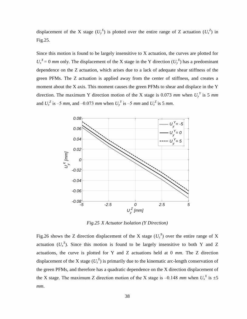
Since this motion is found to be largely insensitive to X actuation, the curves are plotted for

UxX

= 0 mm only. The displacement of the X stage in the Y direction (UyX) has a predominant

dependence on the Z actuation, which arises due to a lack of adequate shear stiffness of the

green PFMs. The Z actuation is applied away from the center of stiffness, and creates a

moment about the X axis. This moment causes the green PFMs to shear and displace in the Y

direction. The maximum Y direction motion of the X stage is 0.073 mm when UyY is 5 mm

and UzZ is ‒5 mm, and ‒0.073 mm when Uy

Y is ‒5 mm and Uz

Z is 5 mm.

Fig.25 X Actuator Isolation (Y Direction)

Fig.26 shows the Z direction displacement of the X stage (UzX) over the entire range of X

actuation (UxX). Since this motion is found to be largely insensitive to both Y and Z

actuations, the curve is plotted for Y and Z actuations held at 0 mm. The Z direction

displacement of the X stage (UzX) is primarily due to the kinematic arc-length conservation of

the green PFMs, and therefore has a quadratic dependence on the X direction displacement of

the X stage. The maximum Z direction motion of the X stage is ‒0.148 mm when UxX is ±5

mm.

-5 -2.5 0 2.5 5-0.08

-0.06

-0.04

-0.02

0

0.02

0.04

0.06

0.08

Uz

Z [mm]

Uy X

[m

m]

Uy

Y= -5

Uy

Y= 0

Uy

Y= 5

39

Fig.26 X Actuator Isolation (Z Direction)

In an XYZ flexure mechanism, all rotations are undesired and represent parasitic errors.

Fig.27 shows the XYZ stage rotations about the X direction (xXYZ

) over the entire range of Y

actuation for three different Z actuations. The rotation varies primarily with Y and Z

actuations, which produce twisting moments at the XYZ stage. It is largely insensitive to X

actuation because the X direction force cannot create a moment about the X axis. Since this

rotation is found to be largely insensitive to X actuation (UxX), the curves are plotted for Ux

X

held at 0 mm. The rotation is linear with Z actuation because it is allowed by the relatively

low torsional stiffness of the red PFMs. As described earlier, the Z actuation causes a

moment about the X axis that is directly proportional to Z displacement. The red PFMs have

a constant torsional stiffness with Z actuation, and therefore deflect linearly with the

displacement. Similarly, the Y actuation produces a moment about the X axis. However, the

X rotation has a nonlinear component with respect to Y actuation. This is because the

torsional stiffness of the red PFMs decreases with Y displacement. This decrease in stiffness

allows additional rotation as can be seen by the increasing slope of the lines in Fig.27.

-5 -2.5 0 2.5 5-0.16

-0.14

-0.12

-0.1

-0.08

-0.06

-0.04

-0.02

0

0.02

Ux

X [mm]

Uz X

[m

m]

Uy

Y = U

z

Z = 0

40

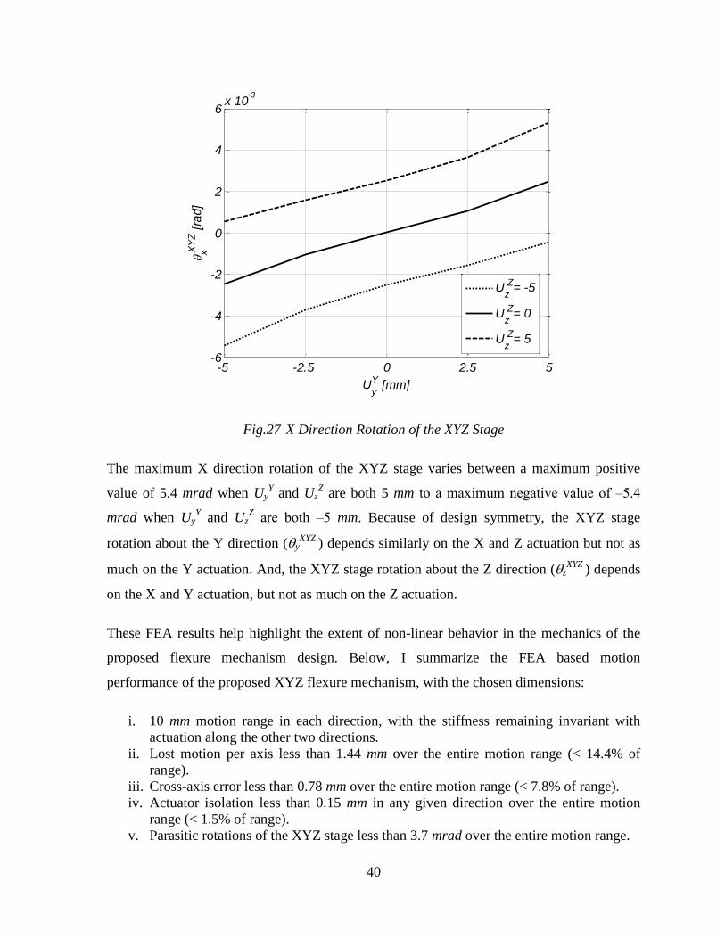
Fig.27 X Direction Rotation of the XYZ Stage

The maximum X direction rotation of the XYZ stage varies between a maximum positive

value of 5.4 mrad when UyY and Uz

Z are both 5 mm to a maximum negative value of ‒5.4

mrad when UyY and Uz

Z are both ‒5 mm. Because of design symmetry, the XYZ stage

rotation about the Y direction (yXYZ

) depends similarly on the X and Z actuation but not as

much on the Y actuation. And, the XYZ stage rotation about the Z direction (zXYZ

) depends

on the X and Y actuation, but not as much on the Z actuation.

These FEA results help highlight the extent of non-linear behavior in the mechanics of the

proposed flexure mechanism design. Below, I summarize the FEA based motion

performance of the proposed XYZ flexure mechanism, with the chosen dimensions:

i. 10 mm motion range in each direction, with the stiffness remaining invariant with

actuation along the other two directions.

ii. Lost motion per axis less than 1.44 mm over the entire motion range (< 14.4% of

range).

iii. Cross-axis error less than 0.78 mm over the entire motion range (< 7.8% of range).

iv. Actuator isolation less than 0.15 mm in any given direction over the entire motion

range (< 1.5% of range).

v. Parasitic rotations of the XYZ stage less than 3.7 mrad over the entire motion range.

-5 -2.5 0 2.5 5-6

-4

-2

0

2

4

6x 10

-3

Uy

Y [mm]

x X

YZ [

rad]

Uz

Z= -5

Uz

Z= 0

Uz

Z= 5

41

4.3 Mechanism CAD Design

As described in the previous chapter on conceptual design, the XYZ flexure mechanism

cannot be manufactured monolithically from a single block of raw material. Therefore, it was

designed in a modular fashion to allow for accurate and repeatable manufacturing and

assembly. Extending from the lessons learned through the design, fabrication, and assembly

of the first two prototypes, I focused on minimizing mass and total number of parts while

simultaneously increasing the alignment accuracy of the entire assembly.

Ground

Corner

Mount

PFMs

Dowel

HolesScrew

Holes

Mounting

Brackets

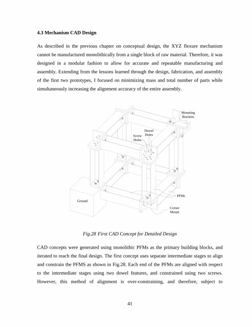
Fig.28 First CAD Concept for Detailed Design

CAD concepts were generated using monolithic PFMs as the primary building blocks, and

iterated to reach the final design. The first concept uses separate intermediate stages to align

and constrain the PFMS as shown in Fig.28. Each end of the PFMs are aligned with respect

to the intermediate stages using two dowel features, and constrained using two screws.

However, this method of alignment is over-constraining, and therefore, subject to

42

manufacturing tolerances. Furthermore, assembly of the mechanism is cumbersome because

the dowel pins must be pressed after all of the pieces are aligned.

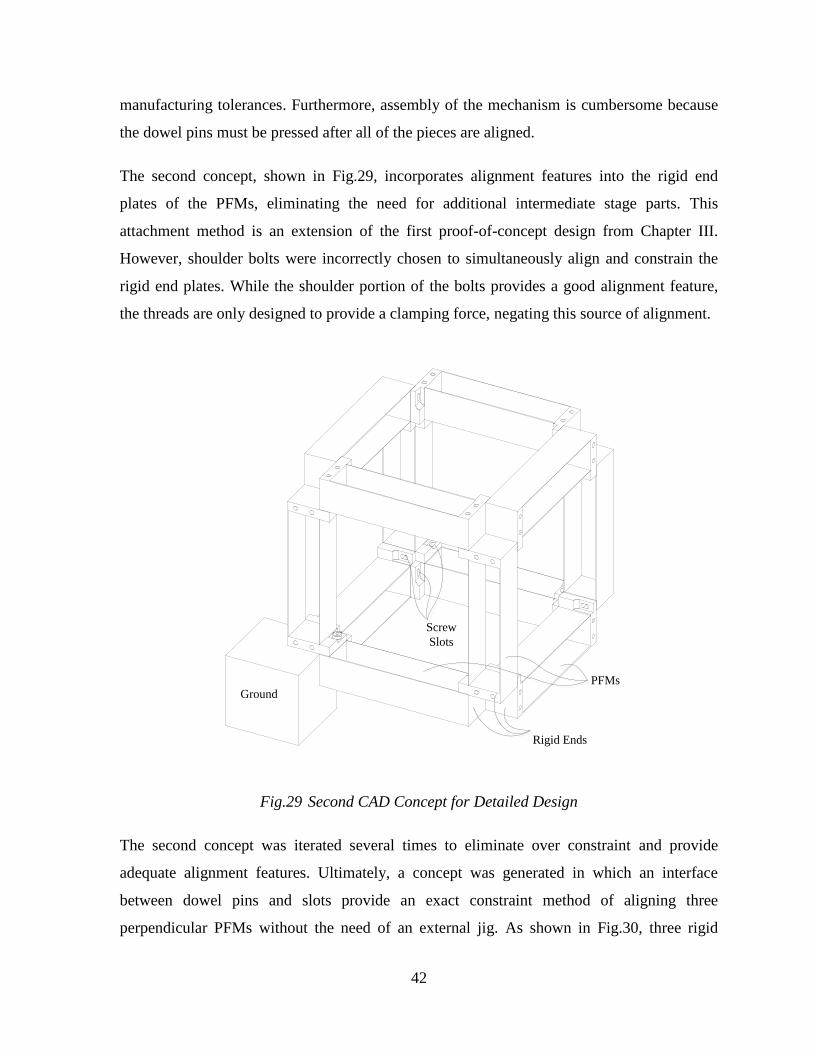
The second concept, shown in Fig.29, incorporates alignment features into the rigid end

plates of the PFMs, eliminating the need for additional intermediate stage parts. This

attachment method is an extension of the first proof-of-concept design from Chapter III.

However, shoulder bolts were incorrectly chosen to simultaneously align and constrain the

rigid end plates. While the shoulder portion of the bolts provides a good alignment feature,

the threads are only designed to provide a clamping force, negating this source of alignment.

GroundPFMs

Rigid Ends

Screw

Slots

Fig.29 Second CAD Concept for Detailed Design

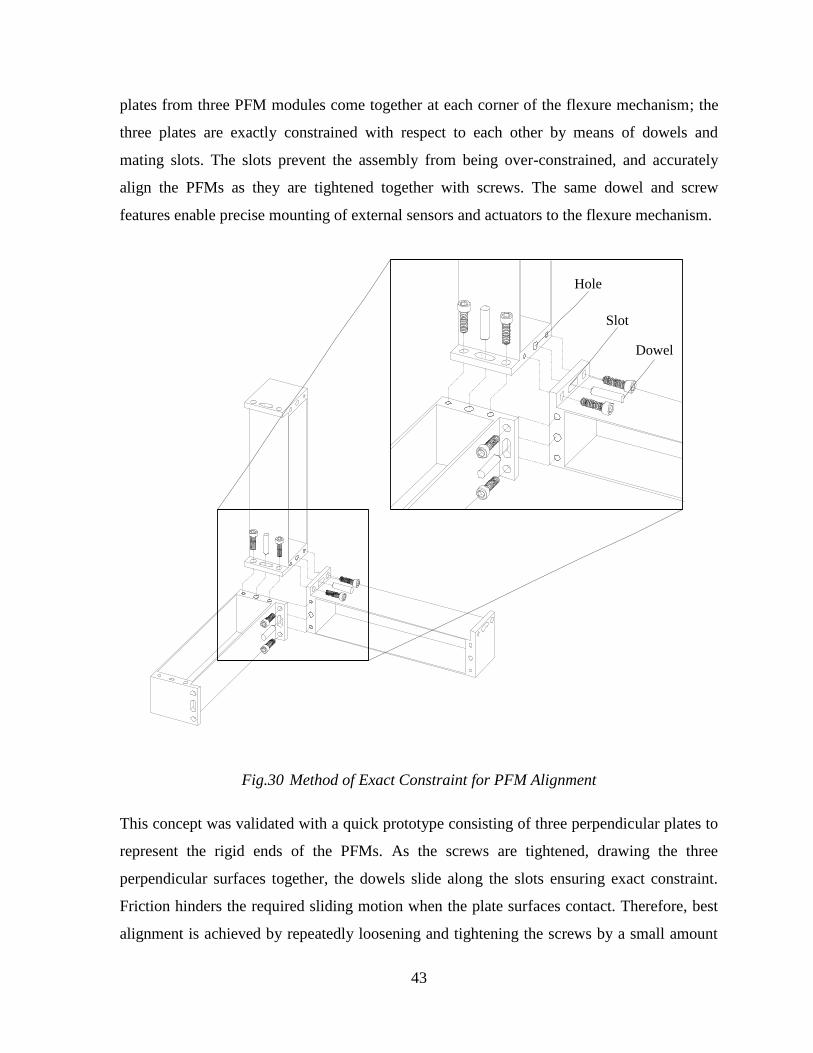
The second concept was iterated several times to eliminate over constraint and provide

adequate alignment features. Ultimately, a concept was generated in which an interface

between dowel pins and slots provide an exact constraint method of aligning three

perpendicular PFMs without the need of an external jig. As shown in Fig.30, three rigid

43

plates from three PFM modules come together at each corner of the flexure mechanism; the

three plates are exactly constrained with respect to each other by means of dowels and

mating slots. The slots prevent the assembly from being over-constrained, and accurately

align the PFMs as they are tightened together with screws. The same dowel and screw

features enable precise mounting of external sensors and actuators to the flexure mechanism.

Dowel

Slot

Hole

Fig.30 Method of Exact Constraint for PFM Alignment

This concept was validated with a quick prototype consisting of three perpendicular plates to

represent the rigid ends of the PFMs. As the screws are tightened, drawing the three

perpendicular surfaces together, the dowels slide along the slots ensuring exact constraint.

Friction hinders the required sliding motion when the plate surfaces contact. Therefore, best

alignment is achieved by repeatedly loosening and tightening the screws by a small amount

44

until no further relative motion between the plates can be seen. Lubricating oil can also aid in

this process.

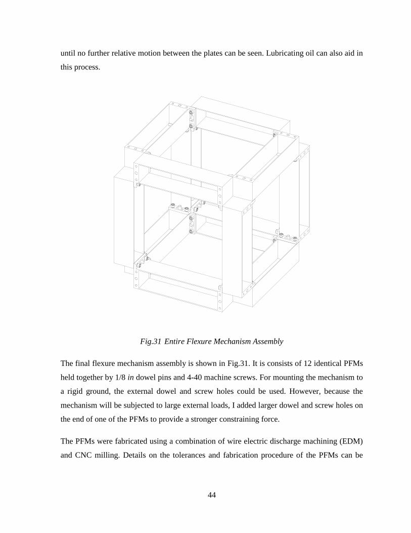
Fig.31 Entire Flexure Mechanism Assembly

The final flexure mechanism assembly is shown in Fig.31. It is consists of 12 identical PFMs

held together by 1/8 in dowel pins and 4-40 machine screws. For mounting the mechanism to

a rigid ground, the external dowel and screw holes could be used. However, because the

mechanism will be subjected to large external loads, I added larger dowel and screw holes on

the end of one of the PFMs to provide a stronger constraining force.

The PFMs were fabricated using a combination of wire electric discharge machining (EDM)

and CNC milling. Details on the tolerances and fabrication procedure of the PFMs can be

45

found in APPENDIX A. Design of an experimental setup, as well as a nanopositioning setup,

is discussed in the subsequent chapters.

46

CHAPTER V

Experimental Validation

5.1 Design of Experiment

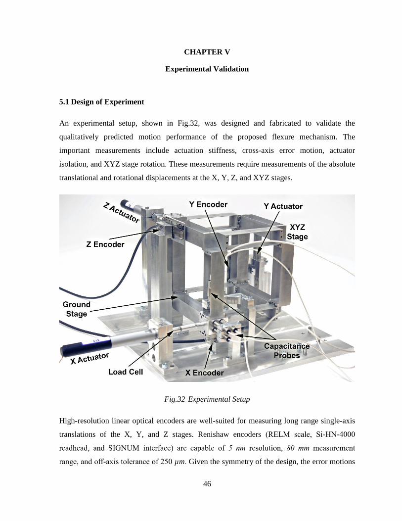
An experimental setup, shown in Fig.32, was designed and fabricated to validate the

qualitatively predicted motion performance of the proposed flexure mechanism. The

important measurements include actuation stiffness, cross-axis error motion, actuator

isolation, and XYZ stage rotation. These measurements require measurements of the absolute

translational and rotational displacements at the X, Y, Z, and XYZ stages.

Fig.32 Experimental Setup

High-resolution linear optical encoders are well-suited for measuring long range single-axis

translations of the X, Y, and Z stages. Renishaw encoders (RELM scale, Si-HN-4000

readhead, and SIGNUM interface) are capable of 5 nm resolution, 80 mm measurement

range, and off-axis tolerance of 250 µm. Given the symmetry of the design, the error motions

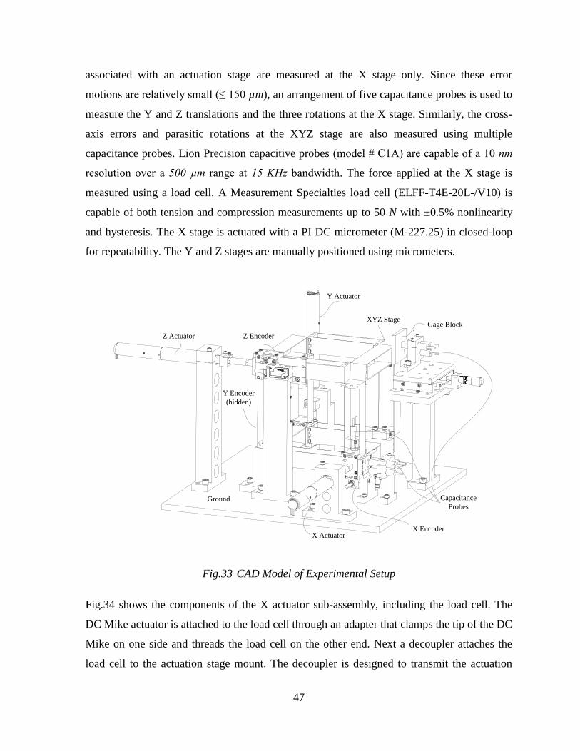
47

associated with an actuation stage are measured at the X stage only. Since these error

motions are relatively small (≤ 150 µm), an arrangement of five capacitance probes is used to

measure the Y and Z translations and the three rotations at the X stage. Similarly, the cross-

axis errors and parasitic rotations at the XYZ stage are also measured using multiple

capacitance probes. Lion Precision capacitive probes (model # C1A) are capable of a 10 nm

resolution over a 500 µm range at 15 KHz bandwidth. The force applied at the X stage is

measured using a load cell. A Measurement Specialties load cell (ELFF-T4E-20L-/V10) is

capable of both tension and compression measurements up to 50 N with ±0.5% nonlinearity

and hysteresis. The X stage is actuated with a PI DC micrometer (M-227.25) in closed-loop

for repeatability. The Y and Z stages are manually positioned using micrometers.

Z Actuator Z Encoder

Capacitance

ProbesGround

X Actuator

Y Actuator

X Encoder

Y Encoder

(hidden)

XYZ StageGage Block`

Fig.33 CAD Model of Experimental Setup

Fig.34 shows the components of the X actuator sub-assembly, including the load cell. The

DC Mike actuator is attached to the load cell through an adapter that clamps the tip of the DC

Mike on one side and threads the load cell on the other end. Next a decoupler attaches the

load cell to the actuation stage mount. The decoupler is designed to transmit the actuation

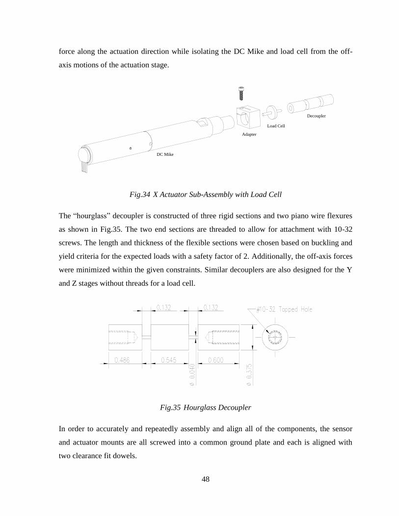
48

force along the actuation direction while isolating the DC Mike and load cell from the off-

axis motions of the actuation stage.

DC Mike

Adapter

Load Cell

Decoupler

Fig.34 X Actuator Sub-Assembly with Load Cell

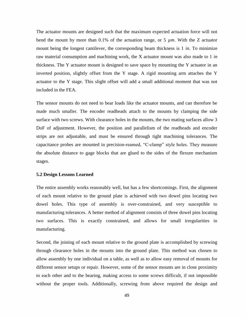
The “hourglass” decoupler is constructed of three rigid sections and two piano wire flexures

as shown in Fig.35. The two end sections are threaded to allow for attachment with 10-32

screws. The length and thickness of the flexible sections were chosen based on buckling and

yield criteria for the expected loads with a safety factor of 2. Additionally, the off-axis forces

were minimized within the given constraints. Similar decouplers are also designed for the Y

and Z stages without threads for a load cell.

Fig.35 Hourglass Decoupler

In order to accurately and repeatedly assembly and align all of the components, the sensor

and actuator mounts are all screwed into a common ground plate and each is aligned with

two clearance fit dowels.

49

The actuator mounts are designed such that the maximum expected actuation force will not

bend the mount by more than 0.1% of the actuation range, or 5 µm. With the Z actuator

mount being the longest cantilever, the corresponding beam thickness is 1 in. To minimize

raw material consumption and machining work, the X actuator mount was also made to 1 in

thickness. The Y actuator mount is designed to save space by mounting the Y actuator in an

inverted position, slightly offset from the Y stage. A rigid mounting arm attaches the Y

actuator to the Y stage. This slight offset will add a small additional moment that was not

included in the FEA.

The sensor mounts do not need to bear loads like the actuator mounts, and can therefore be

made much smaller. The encoder readheads attach to the mounts by clamping the side

surface with two screws. With clearance holes in the mounts, the two mating surfaces allow 3

DoF of adjustment. However, the position and parallelism of the readheads and encoder

strips are not adjustable, and must be ensured through tight machining tolerances. The

capacitance probes are mounted in precision-reamed, “C-clamp” style holes. They measure

the absolute distance to gage blocks that are glued to the sides of the flexure mechanism

stages.

5.2 Design Lessons Learned

The entire assembly works reasonably well, but has a few shortcomings. First, the alignment

of each mount relative to the ground plate is achieved with two dowel pins locating two

dowel holes. This type of assembly is over-constrained, and very susceptible to

manufacturing tolerances. A better method of alignment consists of three dowel pins locating

two surfaces. This is exactly constrained, and allows for small irregularities in

manufacturing.

Second, the joining of each mount relative to the ground plate is accomplished by screwing

through clearance holes in the mounts into the ground plate. This method was chosen to

allow assembly by one individual on a table, as well as to allow easy removal of mounts for

different sensor setups or repair. However, some of the sensor mounts are in close proximity

to each other and to the bearing, making access to some screws difficult, if not impossible

without the proper tools. Additionally, screwing from above required the design and

50

fabrication of mounting tabs on every mount which greatly increased the design complexity,

fabrication time and cost, and material waste. To overcome all of these drawbacks, the

mounting designs could all be altered to simple, rectangular extrusions with screws coming

up through the base into each mount.

Next, as previously described, the encoder readhead mounts do not allow for the full 5 DoF

adjustments necessary to precisely align the readhead to the encoder stip. With the stacked

tolerances from the readhead, readhead mount, ground, bearing mount, bearing PFM,

encoder strip mount, and encoder strip, the misalignment due to manufacturing tolerances

was too great to even use the optical encoders as-is. The mounting dowels were removed and

shims were used to attain proper alignment, but this resulted in several hours of work for

each sensor every time the setup was moved. To alleviate this problem, the mount should be

designed with no alignment dowels, but instead with additional screws to allow the additional

DoF. One example is to have one screw clamping the mount and three screws pressing

against the mount to adjust height, pitch, and roll. Combined with the three DoF allowed

between the mount and the ground, all 6 DoF would be available for fine adjustment with

screws.

Another source of difficulty and uncertainty came from the hourglass flexures used to

separate the actuators from the nonlinear motion of the bearing. While designed well in

theory, the construction of the hourglass flexures was difficult to create from solid material.

The resulting flexures were made from four separate pieces that did not remain solid

throughout the series of experiments. This resulted in inconsistencies between tests. A good

solution is to determine a fabrication method that would allow the manufacturing of the

flexures from a single piece of material, or to otherwise permanently join the flexible and

rigid sections.

Finally, the C-clamps used to mount the actuators and cap probes showed signs of fatigue

over time, and did not provide strong, even clamping force around the delicate bodies of the

actuators and cap probes. A simple solution is to replace the C-clamps with split-rings and set

screws. This would provide a more durable mounting platform that can provide greater

clamping force without damaging the equipment.

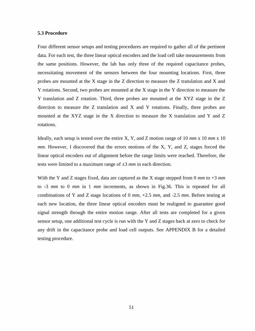
51

5.3 Procedure

Four different sensor setups and testing procedures are required to gather all of the pertinent

data. For each test, the three linear optical encoders and the load cell take measurements from

the same positions. However, the lab has only three of the required capacitance probes,

necessitating movement of the sensors between the four mounting locations. First, three

probes are mounted at the X stage in the Z direction to measure the Z translation and X and

Y rotations. Second, two probes are mounted at the X stage in the Y direction to measure the

Y translation and Z rotation. Third, three probes are mounted at the XYZ stage in the Z

direction to measure the Z translation and X and Y rotations. Finally, three probes are

mounted at the XYZ stage in the X direction to measure the X translation and Y and Z

rotations.

Ideally, each setup is tested over the entire X, Y, and Z motion range of 10 mm x 10 mm x 10

mm. However, I discovered that the errors motions of the X, Y, and Z, stages forced the

linear optical encoders out of alignment before the range limits were reached. Therefore, the

tests were limited to a maximum range of ±3 mm in each direction.

With the Y and Z stages fixed, data are captured as the X stage stepped from 0 mm to +3 mm

to -3 mm to 0 mm in 1 mm increments, as shown in Fig.36. This is repeated for all

combinations of Y and Z stage locations of 0 mm, +2.5 mm, and -2.5 mm. Before testing at

each new location, the three linear optical encoders must be realigned to guarantee good

signal strength through the entire motion range. After all tests are completed for a given

sensor setup, one additional test cycle is run with the Y and Z stages back at zero to check for

any drift in the capacitance probe and load cell outputs. See APPENDIX B for a detailed

testing procedure.

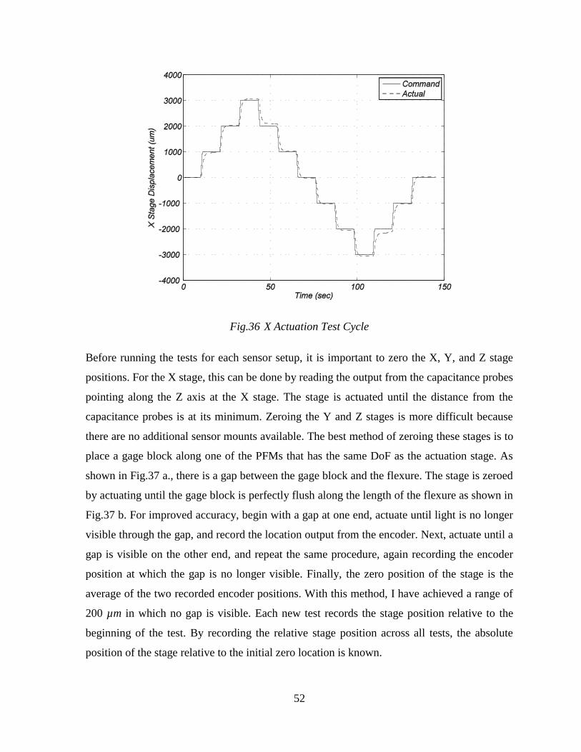
52

Fig.36 X Actuation Test Cycle

Before running the tests for each sensor setup, it is important to zero the X, Y, and Z stage

positions. For the X stage, this can be done by reading the output from the capacitance probes

pointing along the Z axis at the X stage. The stage is actuated until the distance from the

capacitance probes is at its minimum. Zeroing the Y and Z stages is more difficult because

there are no additional sensor mounts available. The best method of zeroing these stages is to

place a gage block along one of the PFMs that has the same DoF as the actuation stage. As

shown in Fig.37 a., there is a gap between the gage block and the flexure. The stage is zeroed

by actuating until the gage block is perfectly flush along the length of the flexure as shown in

Fig.37 b. For improved accuracy, begin with a gap at one end, actuate until light is no longer

visible through the gap, and record the location output from the encoder. Next, actuate until a

gap is visible on the other end, and repeat the same procedure, again recording the encoder

position at which the gap is no longer visible. Finally, the zero position of the stage is the

average of the two recorded encoder positions. With this method, I have achieved a range of

200 µm in which no gap is visible. Each new test records the stage position relative to the

beginning of the test. By recording the relative stage position across all tests, the absolute

position of the stage relative to the initial zero location is known.

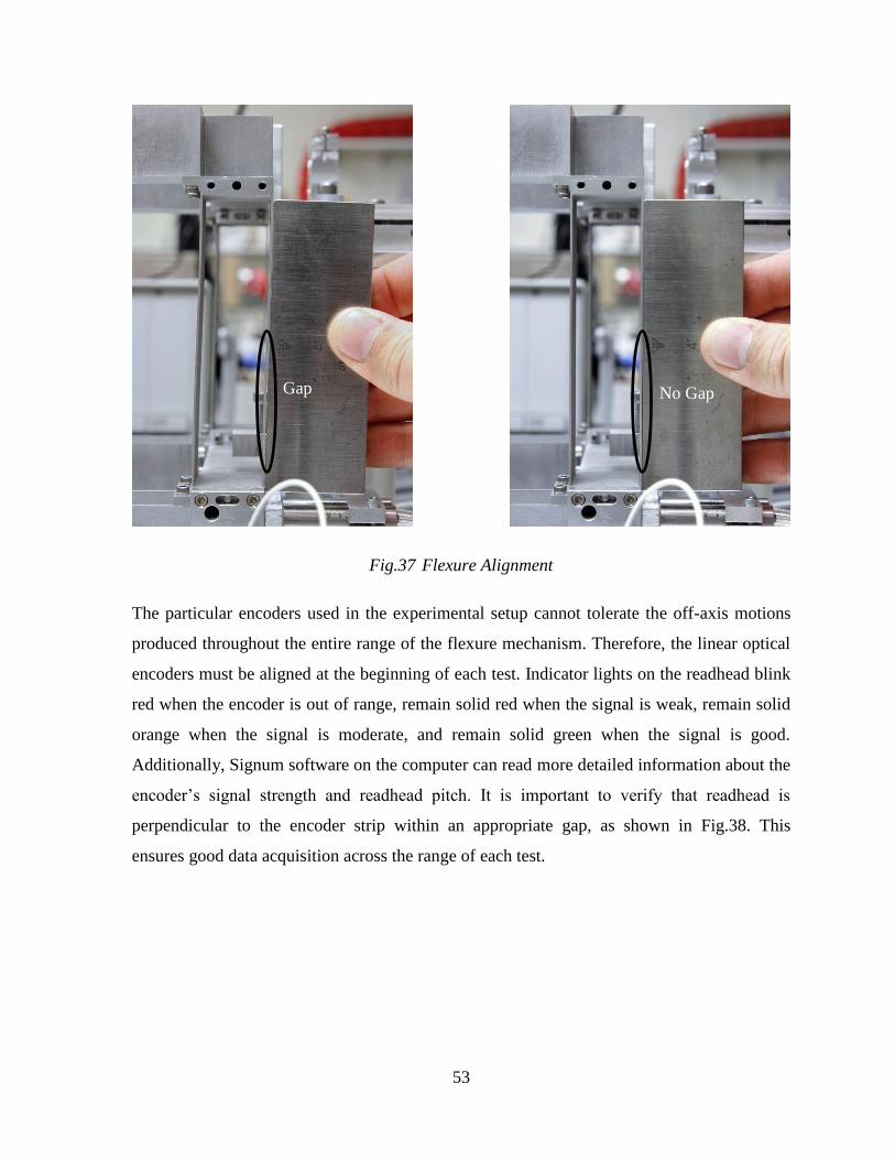
53

Fig.37 Flexure Alignment

The particular encoders used in the experimental setup cannot tolerate the off-axis motions

produced throughout the entire range of the flexure mechanism. Therefore, the linear optical

encoders must be aligned at the beginning of each test. Indicator lights on the readhead blink

red when the encoder is out of range, remain solid red when the signal is weak, remain solid

orange when the signal is moderate, and remain solid green when the signal is good.

Additionally, Signum software on the computer can read more detailed information about the

encoder’s signal strength and readhead pitch. It is important to verify that readhead is

perpendicular to the encoder strip within an appropriate gap, as shown in Fig.38. This

ensures good data acquisition across the range of each test.

Gap No Gap

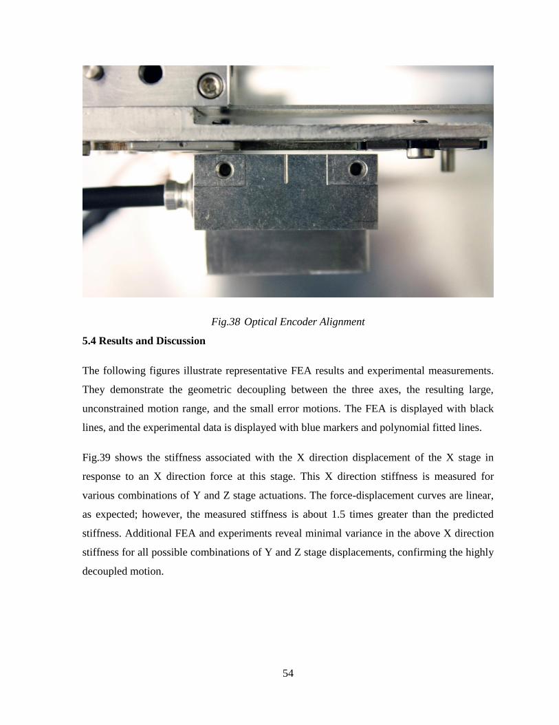
54

Fig.38 Optical Encoder Alignment

5.4 Results and Discussion

The following figures illustrate representative FEA results and experimental measurements.

They demonstrate the geometric decoupling between the three axes, the resulting large,

unconstrained motion range, and the small error motions. The FEA is displayed with black

lines, and the experimental data is displayed with blue markers and polynomial fitted lines.

Fig.39 shows the stiffness associated with the X direction displacement of the X stage in

response to an X direction force at this stage. This X direction stiffness is measured for

various combinations of Y and Z stage actuations. The force-displacement curves are linear,

as expected; however, the measured stiffness is about 1.5 times greater than the predicted

stiffness. Additional FEA and experiments reveal minimal variance in the above X direction

stiffness for all possible combinations of Y and Z stage displacements, confirming the highly

decoupled motion.

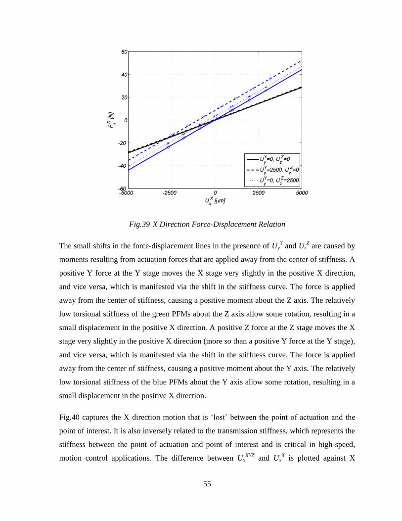
55

Fig.39 X Direction Force-Displacement Relation

The small shifts in the force-displacement lines in the presence of UyY and Uz

Z are caused by

moments resulting from actuation forces that are applied away from the center of stiffness. A

positive Y force at the Y stage moves the X stage very slightly in the positive X direction,

and vice versa, which is manifested via the shift in the stiffness curve. The force is applied

away from the center of stiffness, causing a positive moment about the Z axis. The relatively

low torsional stiffness of the green PFMs about the Z axis allow some rotation, resulting in a

small displacement in the positive X direction. A positive Z force at the Z stage moves the X

stage very slightly in the positive X direction (more so than a positive Y force at the Y stage),

and vice versa, which is manifested via the shift in the stiffness curve. The force is applied

away from the center of stiffness, causing a positive moment about the Y axis. The relatively

low torsional stiffness of the blue PFMs about the Y axis allow some rotation, resulting in a

small displacement in the positive X direction.

Fig.40 captures the X direction motion that is ‘lost’ between the point of actuation and the

point of interest. It is also inversely related to the transmission stiffness, which represents the

stiffness between the point of actuation and point of interest and is critical in high-speed,

motion control applications. The difference between UxXYZ

and UxX is plotted against X

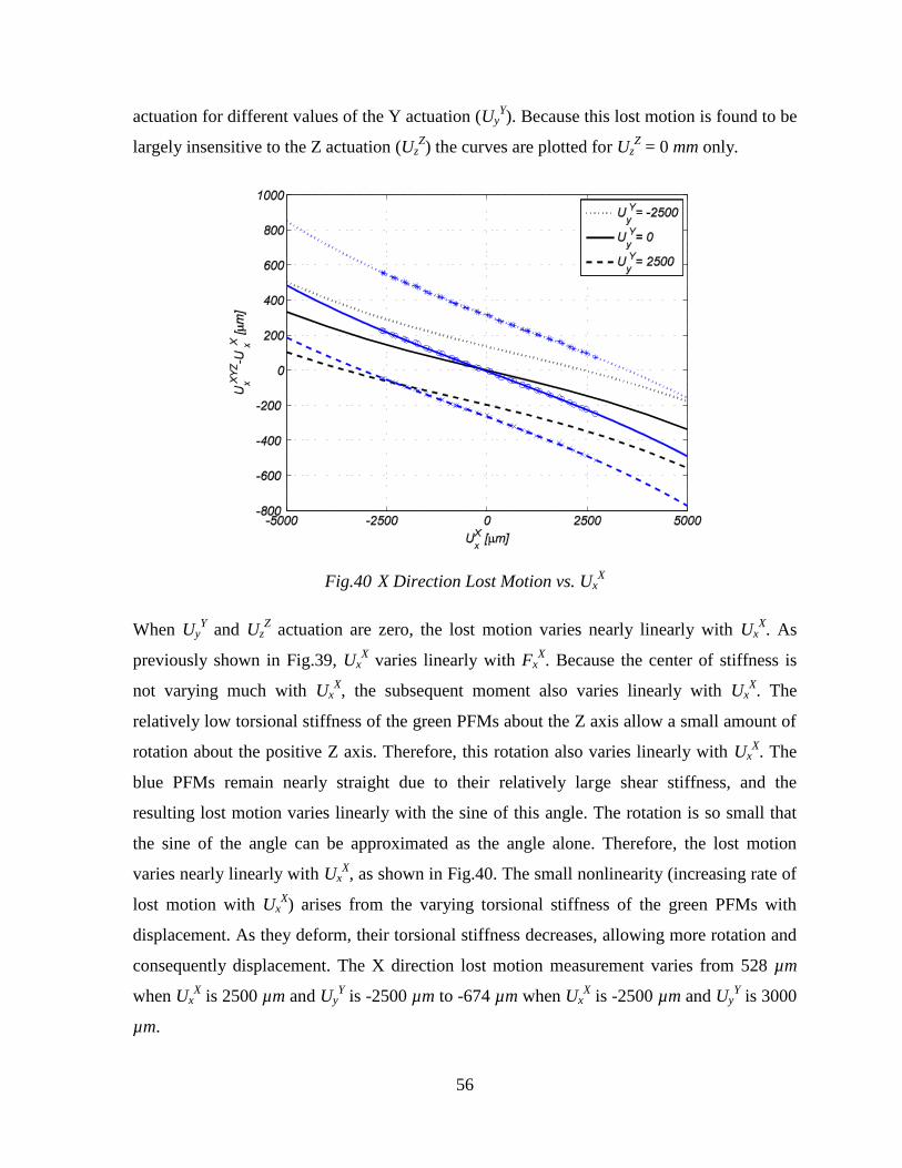
56

actuation for different values of the Y actuation (UyY). Because this lost motion is found to be

largely insensitive to the Z actuation (UzZ) the curves are plotted for Uz

Z = 0 mm only.

Fig.40 X Direction Lost Motion vs. UxX

When UyY and Uz

Z actuation are zero, the lost motion varies nearly linearly with Ux

X. As

previously shown in Fig.39, UxX varies linearly with Fx

X. Because the center of stiffness is

not varying much with UxX, the subsequent moment also varies linearly with Ux

X. The

relatively low torsional stiffness of the green PFMs about the Z axis allow a small amount of

rotation about the positive Z axis. Therefore, this rotation also varies linearly with UxX. The

blue PFMs remain nearly straight due to their relatively large shear stiffness, and the

resulting lost motion varies linearly with the sine of this angle. The rotation is so small that

the sine of the angle can be approximated as the angle alone. Therefore, the lost motion

varies nearly linearly with UxX, as shown in Fig.40. The small nonlinearity (increasing rate of

lost motion with UxX) arises from the varying torsional stiffness of the green PFMs with

displacement. As they deform, their torsional stiffness decreases, allowing more rotation and

consequently displacement. The X direction lost motion measurement varies from 528 µm

when UxX is 2500 µm and Uy

Y is -2500 µm to -674 µm when Ux

X is -2500 µm and Uy

Y is 3000

µm.

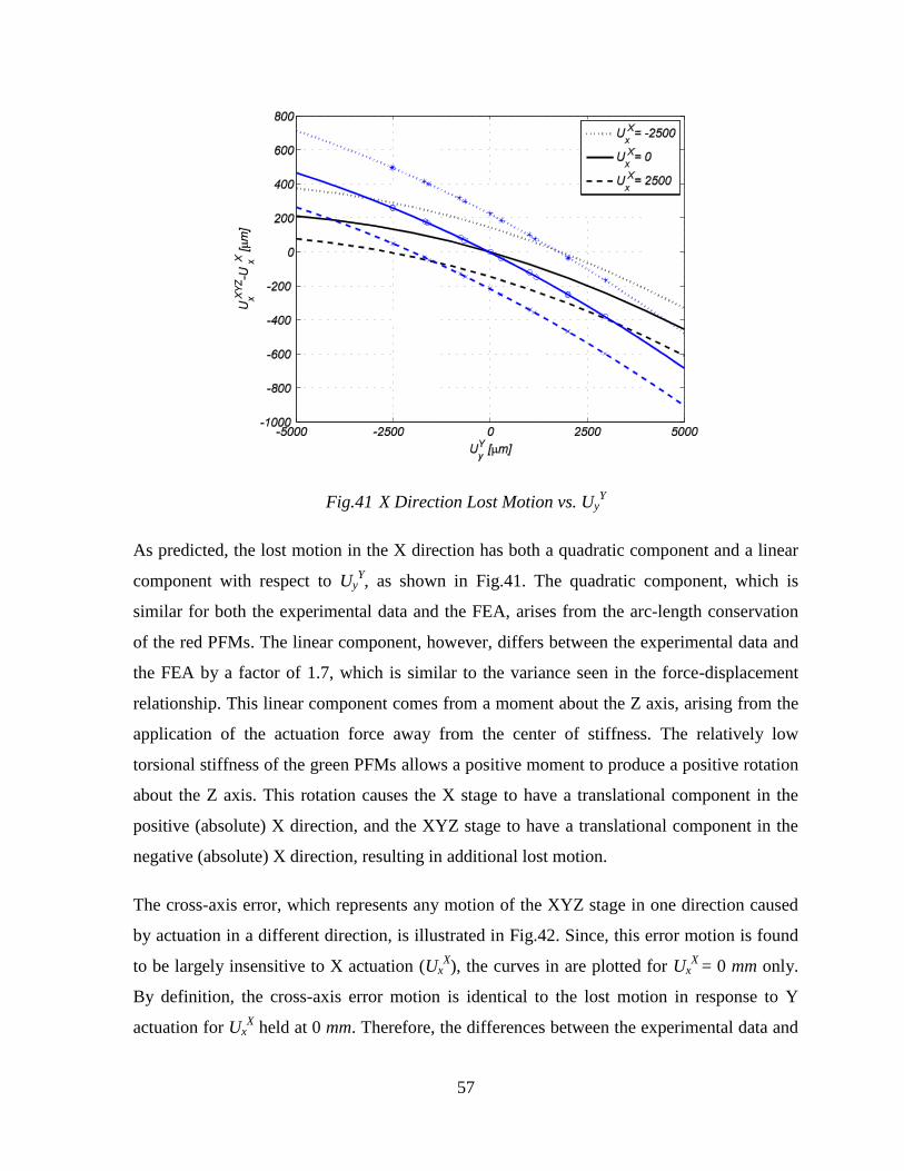
57

Fig.41 X Direction Lost Motion vs. UyY

As predicted, the lost motion in the X direction has both a quadratic component and a linear

component with respect to UyY, as shown in Fig.41. The quadratic component, which is

similar for both the experimental data and the FEA, arises from the arc-length conservation

of the red PFMs. The linear component, however, differs between the experimental data and

the FEA by a factor of 1.7, which is similar to the variance seen in the force-displacement

relationship. This linear component comes from a moment about the Z axis, arising from the

application of the actuation force away from the center of stiffness. The relatively low

torsional stiffness of the green PFMs allows a positive moment to produce a positive rotation

about the Z axis. This rotation causes the X stage to have a translational component in the

positive (absolute) X direction, and the XYZ stage to have a translational component in the

negative (absolute) X direction, resulting in additional lost motion.

The cross-axis error, which represents any motion of the XYZ stage in one direction caused

by actuation in a different direction, is illustrated in Fig.42. Since, this error motion is found

to be largely insensitive to X actuation (UxX), the curves in are plotted for Ux

X = 0 mm only.

By definition, the cross-axis error motion is identical to the lost motion in response to Y

actuation for UxX held at 0 mm. Therefore, the differences between the experimental data and

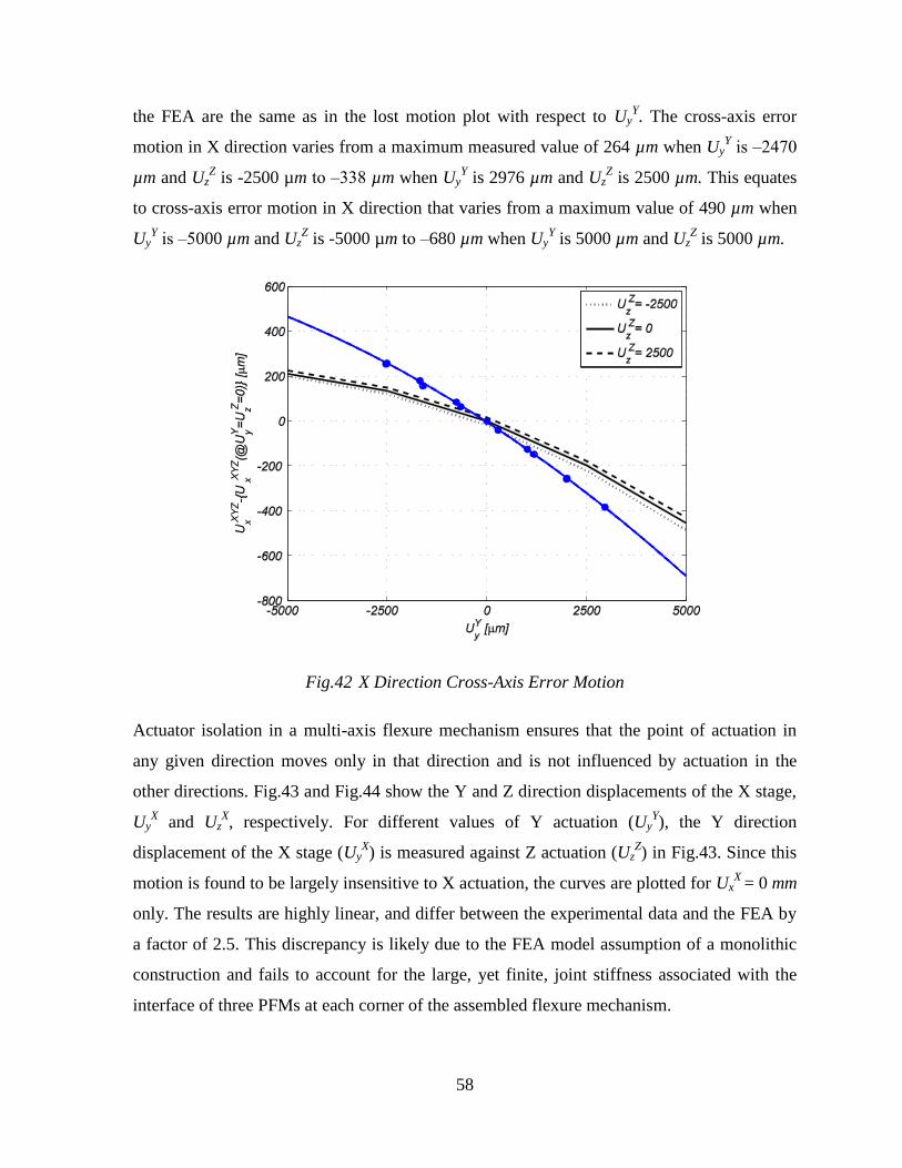
58

the FEA are the same as in the lost motion plot with respect to UyY. The cross-axis error

motion in X direction varies from a maximum measured value of 264 µm when UyY is ‒2470

µm and UzZ is -2500 µm to ‒338 µm when Uy

Y is 2976 µm and Uz

Z is 2500 µm. This equates

to cross-axis error motion in X direction that varies from a maximum value of 490 µm when

UyY is ‒5000 µm and Uz

Z is -5000 µm to ‒680 µm when Uy

Y is 5000 µm and Uz

Z is 5000 µm.

Fig.42 X Direction Cross-Axis Error Motion

Actuator isolation in a multi-axis flexure mechanism ensures that the point of actuation in

any given direction moves only in that direction and is not influenced by actuation in the

other directions. Fig.43 and Fig.44 show the Y and Z direction displacements of the X stage,

UyX and Uz

X, respectively. For different values of Y actuation (Uy

Y), the Y direction

displacement of the X stage (UyX) is measured against Z actuation (Uz

Z) in Fig.43. Since this

motion is found to be largely insensitive to X actuation, the curves are plotted for UxX

= 0 mm

only. The results are highly linear, and differ between the experimental data and the FEA by

a factor of 2.5. This discrepancy is likely due to the FEA model assumption of a monolithic

construction and fails to account for the large, yet finite, joint stiffness associated with the

interface of three PFMs at each corner of the assembled flexure mechanism.

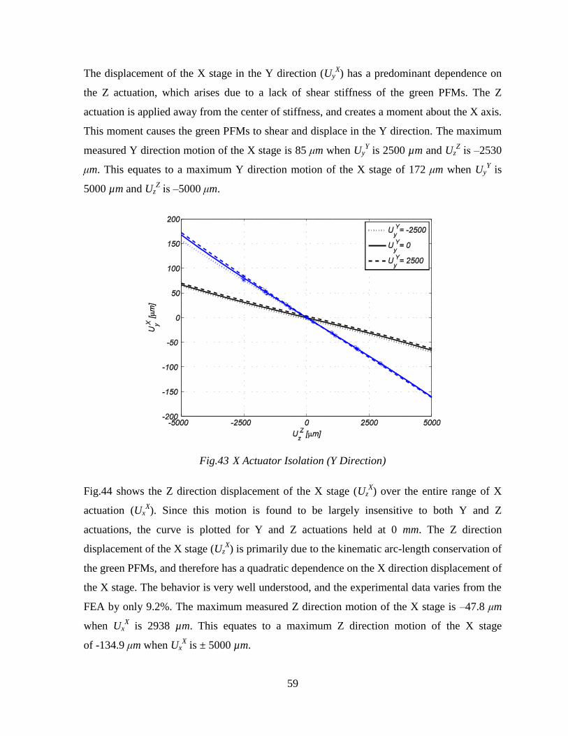
59

The displacement of the X stage in the Y direction (UyX) has a predominant dependence on

the Z actuation, which arises due to a lack of shear stiffness of the green PFMs. The Z

actuation is applied away from the center of stiffness, and creates a moment about the X axis.

This moment causes the green PFMs to shear and displace in the Y direction. The maximum

measured Y direction motion of the X stage is 85 μm when UyY is 2500 µm and Uz

Z is ‒2530

μm. This equates to a maximum Y direction motion of the X stage of 172 μm when UyY is

5000 µm and UzZ is ‒5000 μm.

Fig.43 X Actuator Isolation (Y Direction)

Fig.44 shows the Z direction displacement of the X stage (UzX) over the entire range of X

actuation (UxX). Since this motion is found to be largely insensitive to both Y and Z

actuations, the curve is plotted for Y and Z actuations held at 0 mm. The Z direction

displacement of the X stage (UzX) is primarily due to the kinematic arc-length conservation of

the green PFMs, and therefore has a quadratic dependence on the X direction displacement of

the X stage. The behavior is very well understood, and the experimental data varies from the

FEA by only 9.2%. The maximum measured Z direction motion of the X stage is ‒47.8 μm

when UxX is 2938 µm. This equates to a maximum Z direction motion of the X stage

of -134.9 μm when UxX is ± 5000 µm.

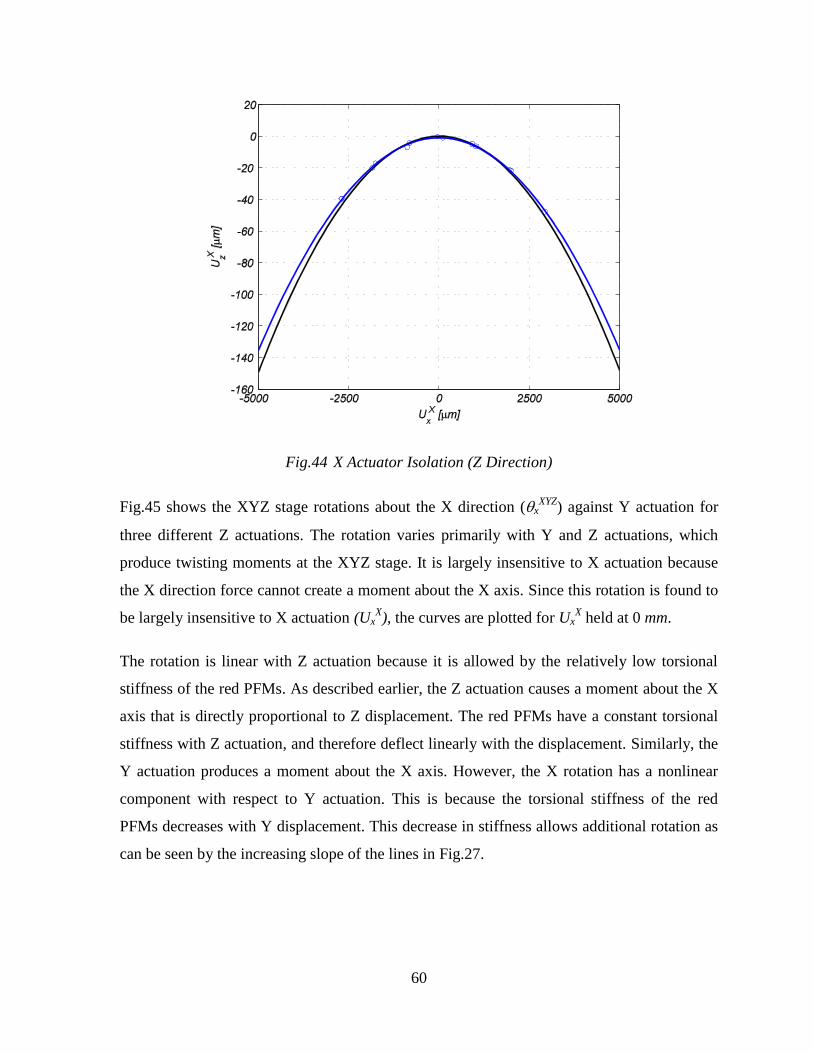
60

Fig.44 X Actuator Isolation (Z Direction)

Fig.45 shows the XYZ stage rotations about the X direction (xXYZ

) against Y actuation for

three different Z actuations. The rotation varies primarily with Y and Z actuations, which

produce twisting moments at the XYZ stage. It is largely insensitive to X actuation because

the X direction force cannot create a moment about the X axis. Since this rotation is found to

be largely insensitive to X actuation (UxX), the curves are plotted for Ux

X held at 0 mm.

The rotation is linear with Z actuation because it is allowed by the relatively low torsional

stiffness of the red PFMs. As described earlier, the Z actuation causes a moment about the X

axis that is directly proportional to Z displacement. The red PFMs have a constant torsional

stiffness with Z actuation, and therefore deflect linearly with the displacement. Similarly, the

Y actuation produces a moment about the X axis. However, the X rotation has a nonlinear

component with respect to Y actuation. This is because the torsional stiffness of the red

PFMs decreases with Y displacement. This decrease in stiffness allows additional rotation as

can be seen by the increasing slope of the lines in Fig.27.

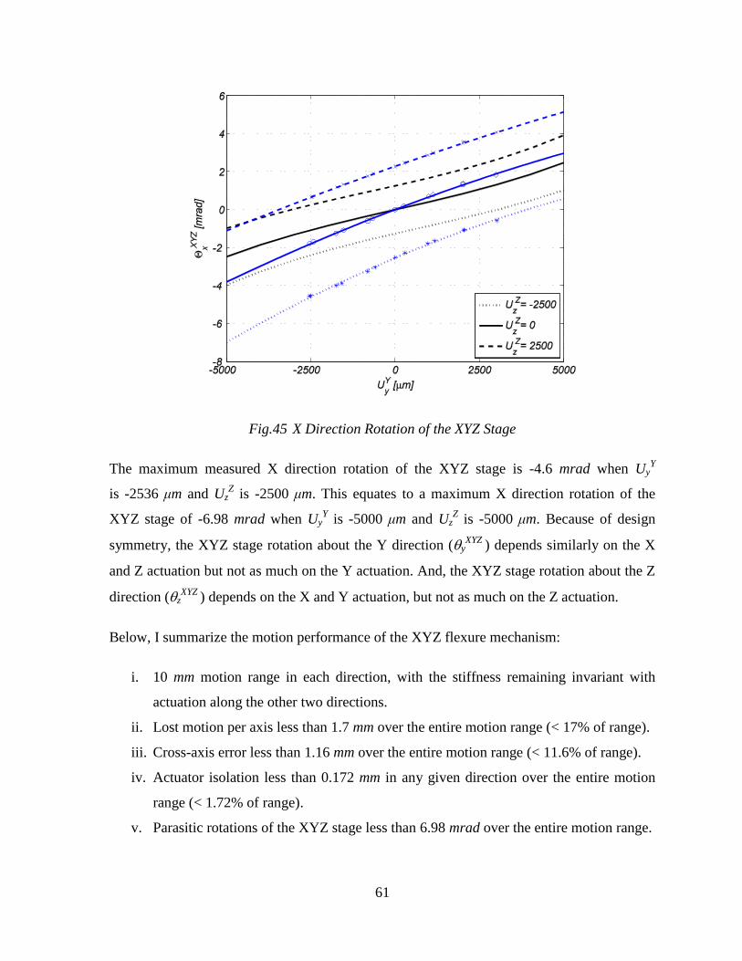
61

Fig.45 X Direction Rotation of the XYZ Stage

The maximum measured X direction rotation of the XYZ stage is -4.6 mrad when UyY

is -2536 μm and UzZ is -2500 μm. This equates to a maximum X direction rotation of the

XYZ stage of -6.98 mrad when UyY is -5000 μm and Uz

Z is -5000 μm. Because of design

symmetry, the XYZ stage rotation about the Y direction (yXYZ

) depends similarly on the X

and Z actuation but not as much on the Y actuation. And, the XYZ stage rotation about the Z

direction (zXYZ

) depends on the X and Y actuation, but not as much on the Z actuation.

Below, I summarize the motion performance of the XYZ flexure mechanism:

i. 10 mm motion range in each direction, with the stiffness remaining invariant with

actuation along the other two directions.

ii. Lost motion per axis less than 1.7 mm over the entire motion range (< 17% of range).

iii. Cross-axis error less than 1.16 mm over the entire motion range (< 11.6% of range).

iv. Actuator isolation less than 0.172 mm in any given direction over the entire motion

range (< 1.72% of range).

v. Parasitic rotations of the XYZ stage less than 6.98 mrad over the entire motion range.

62

Although the experimental data show a greater-than-expected DoF stiffness and a less-than-

expected DoC stiffness, the flexure mechanism still demonstrated geometric decoupling

between the three axes, large motion range, and relatively small error motions. Discrepancies

between the experimental data and the FEA may be due to one or more of the following

shortcomings. Although great care was taken in selecting appropriate FEA parameters, the

element types may include certain assumptions that limit their prediction of rotations

resulting from complex structural loading. Additionally, the mesh density was limited by the

available computational power, and could be improved given more time and resources.

Considering the experimental setup, data collection was limited by the tolerance of the linear

optical encoders to off-axis motions. Encoders with lower resolution, but higher tolerances to

off-axis motion, could be used to collect complete data. Also, the load cell used showed a

significant amount of drift between tests, limiting its trustworthiness. Finally, the bearing

itself has a large, but finite, joint stiffness between PFMs. Relative motion between the ends

of the PFMs, especially sliding motion, would result in errors that are very difficult to

predict.

As previously discussed, the error motions are expected to be significantly reduced if the

actuation force can be applied closer to the center of stiffness. This could be easily done by

fabricating a simple adapter to rigidly mount the actuator to the actuation stage, but in a new

desired location. The benefit of reduced error motions would greatly outweigh the impact of

the added mass.

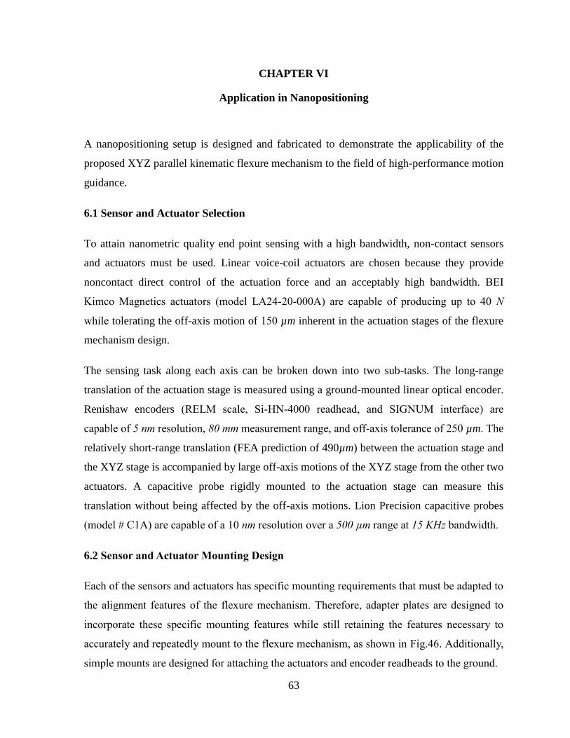
63

CHAPTER VI

Application in Nanopositioning

A nanopositioning setup is designed and fabricated to demonstrate the applicability of the

proposed XYZ parallel kinematic flexure mechanism to the field of high-performance motion

guidance.

6.1 Sensor and Actuator Selection

To attain nanometric quality end point sensing with a high bandwidth, non-contact sensors

and actuators must be used. Linear voice-coil actuators are chosen because they provide

noncontact direct control of the actuation force and an acceptably high bandwidth. BEI

Kimco Magnetics actuators (model LA24-20-000A) are capable of producing up to 40 N

while tolerating the off-axis motion of 150 µm inherent in the actuation stages of the flexure

mechanism design.

The sensing task along each axis can be broken down into two sub-tasks. The long-range

translation of the actuation stage is measured using a ground-mounted linear optical encoder.

Renishaw encoders (RELM scale, Si-HN-4000 readhead, and SIGNUM interface) are

capable of 5 nm resolution, 80 mm measurement range, and off-axis tolerance of 250 µm. The

relatively short-range translation (FEA prediction of 490µm) between the actuation stage and

the XYZ stage is accompanied by large off-axis motions of the XYZ stage from the other two

actuators. A capacitive probe rigidly mounted to the actuation stage can measure this

translation without being affected by the off-axis motions. Lion Precision capacitive probes

(model # C1A) are capable of a 10 nm resolution over a 500 µm range at 15 KHz bandwidth.

6.2 Sensor and Actuator Mounting Design

Each of the sensors and actuators has specific mounting requirements that must be adapted to

the alignment features of the flexure mechanism. Therefore, adapter plates are designed to

incorporate these specific mounting features while still retaining the features necessary to

accurately and repeatedly mount to the flexure mechanism, as shown in Fig.46. Additionally,

simple mounts are designed for attaching the actuators and encoder readheads to the ground.

64

Voice Coil

Actuator

Capacitance

Probe

Linear Optical

Encoder Strip

Fig.46 XYZ Nanopositioner Sensor and Actuator Mounts

Mounting the capacitance probes presents a large problem because of their large distance

away from the actuation stages. Actuation bandwidth is of great importance to

nanopositioning, and therefore mass must be minimized while maintaining sufficient rigidity

and maximizing the first fundamental frequency. I designed a truss structure with a first

fundamental frequency greater than 20 Hz with a maximum stiffness along the capacitance

probe axis. The structure was modified based on both dynamic and static FEA results. Fig.47

shows the displacement of the structure under the three directions of gravitational loading.

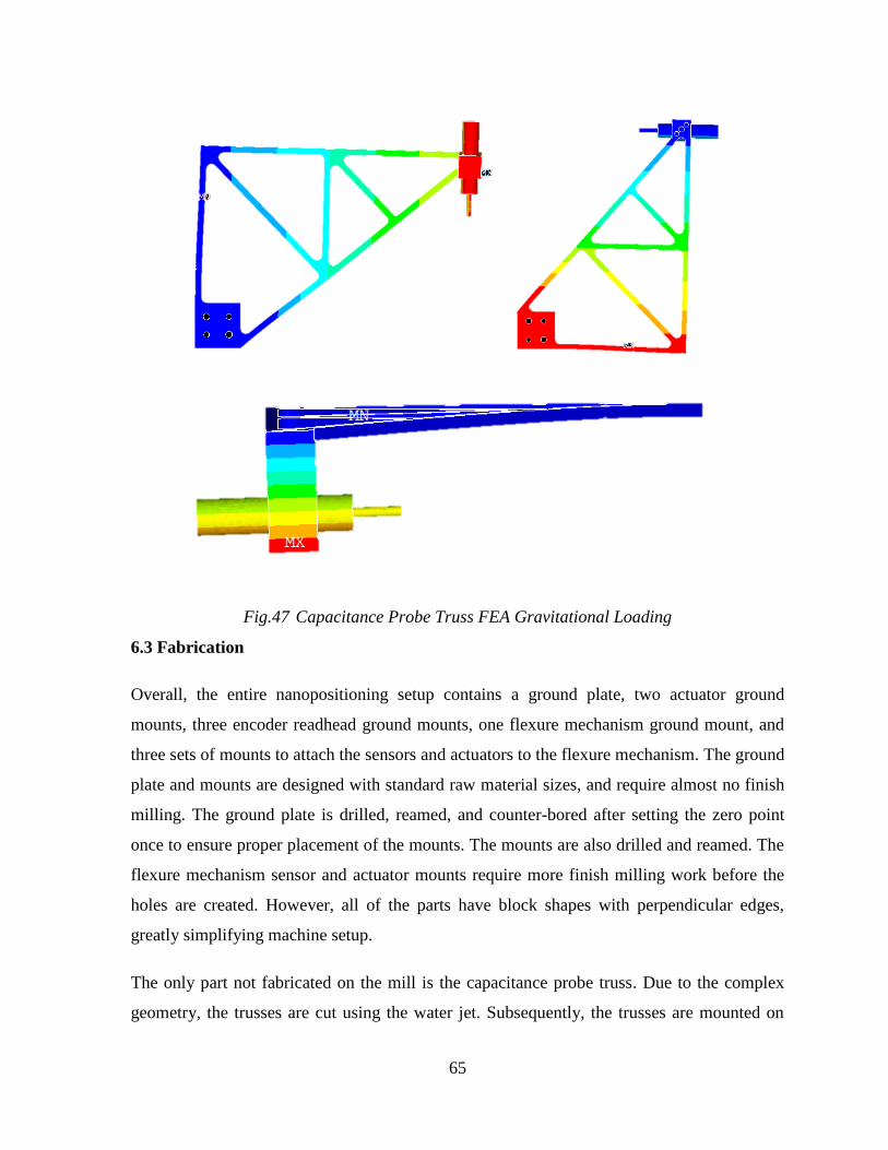
65

Fig.47 Capacitance Probe Truss FEA Gravitational Loading

6.3 Fabrication

Overall, the entire nanopositioning setup contains a ground plate, two actuator ground

mounts, three encoder readhead ground mounts, one flexure mechanism ground mount, and

three sets of mounts to attach the sensors and actuators to the flexure mechanism. The ground

plate and mounts are designed with standard raw material sizes, and require almost no finish

milling. The ground plate is drilled, reamed, and counter-bored after setting the zero point

once to ensure proper placement of the mounts. The mounts are also drilled and reamed. The

flexure mechanism sensor and actuator mounts require more finish milling work before the

holes are created. However, all of the parts have block shapes with perpendicular edges,

greatly simplifying machine setup.

The only part not fabricated on the mill is the capacitance probe truss. Due to the complex

geometry, the trusses are cut using the water jet. Subsequently, the trusses are mounted on

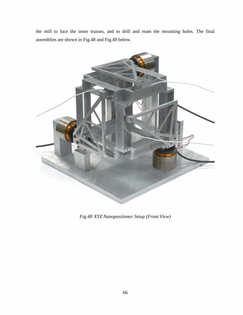
66

the mill to face the inner trusses, and to drill and ream the mounting holes. The final

assemblies are shown in Fig.48 and Fig.49 below.

Fig.48 XYZ Nanopositioner Setup (Front View)

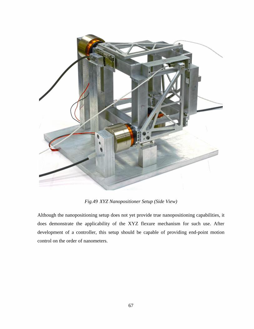
67

Fig.49 XYZ Nanopositioner Setup (Side View)

Although the nanopositioning setup does not yet provide true nanopositioning capabilities, it

does demonstrate the applicability of the XYZ flexure mechanism for such use. After

development of a controller, this setup should be capable of providing end-point motion

control on the order of nanometers.

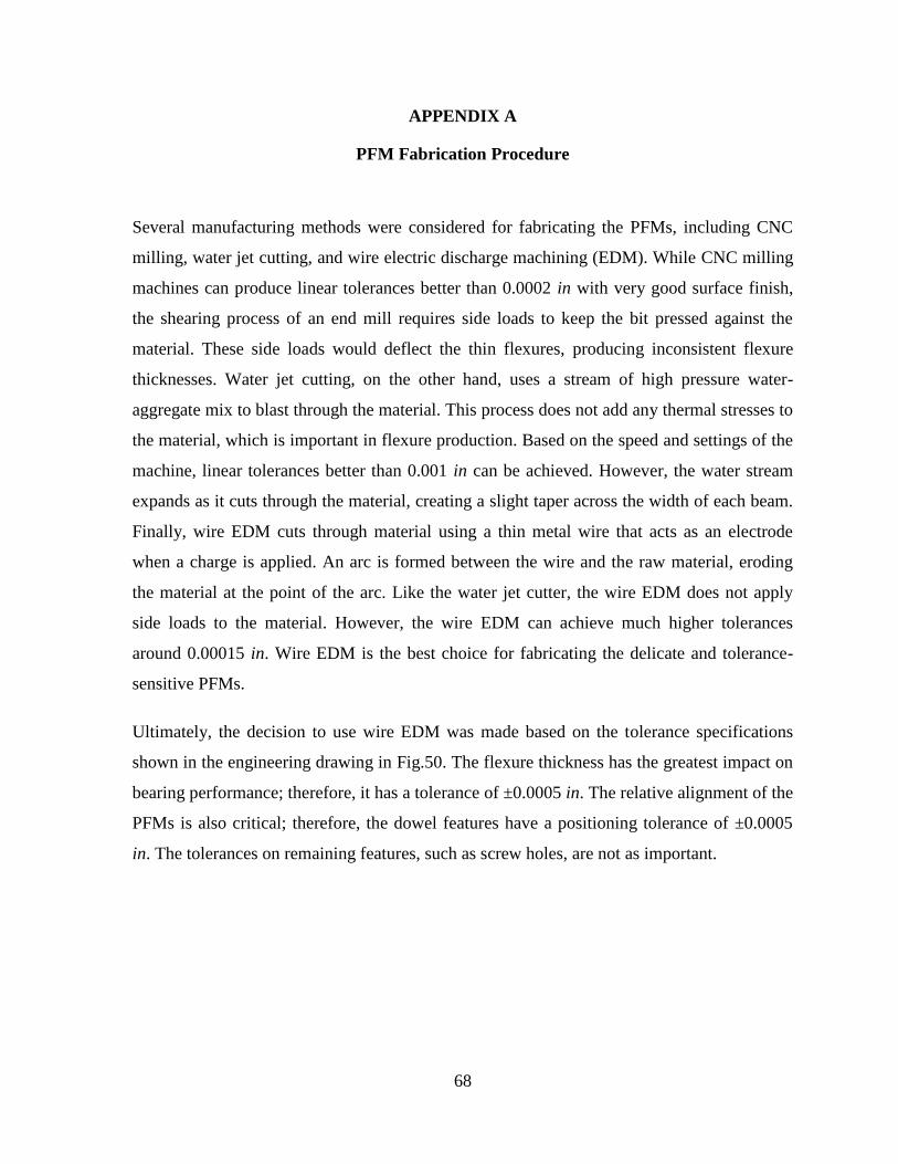
68

APPENDIX A

PFM Fabrication Procedure

Several manufacturing methods were considered for fabricating the PFMs, including CNC

milling, water jet cutting, and wire electric discharge machining (EDM). While CNC milling

machines can produce linear tolerances better than 0.0002 in with very good surface finish,

the shearing process of an end mill requires side loads to keep the bit pressed against the

material. These side loads would deflect the thin flexures, producing inconsistent flexure

thicknesses. Water jet cutting, on the other hand, uses a stream of high pressure water-

aggregate mix to blast through the material. This process does not add any thermal stresses to

the material, which is important in flexure production. Based on the speed and settings of the

machine, linear tolerances better than 0.001 in can be achieved. However, the water stream

expands as it cuts through the material, creating a slight taper across the width of each beam.

Finally, wire EDM cuts through material using a thin metal wire that acts as an electrode

when a charge is applied. An arc is formed between the wire and the raw material, eroding

the material at the point of the arc. Like the water jet cutter, the wire EDM does not apply

side loads to the material. However, the wire EDM can achieve much higher tolerances

around 0.00015 in. Wire EDM is the best choice for fabricating the delicate and tolerance-

sensitive PFMs.

Ultimately, the decision to use wire EDM was made based on the tolerance specifications

shown in the engineering drawing in Fig.50. The flexure thickness has the greatest impact on

bearing performance; therefore, it has a tolerance of ±0.0005 in. The relative alignment of the

PFMs is also critical; therefore, the dowel features have a positioning tolerance of ±0.0005

in. The tolerances on remaining features, such as screw holes, are not as important.

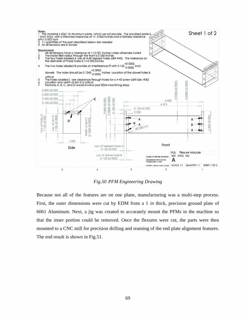
69

Fig.50 PFM Engineering Drawing

Because not all of the features are on one plane, manufacturing was a multi-step process.

First, the outer dimensions were cut by EDM from a 1 in thick, precision ground plate of

6061 Aluminum. Next, a jig was created to accurately mount the PFMs in the machine so

that the inner portion could be removed. Once the flexures were cut, the parts were then

mounted to a CNC mill for precision drilling and reaming of the end plate alignment features.

The end result is shown in Fig.51.

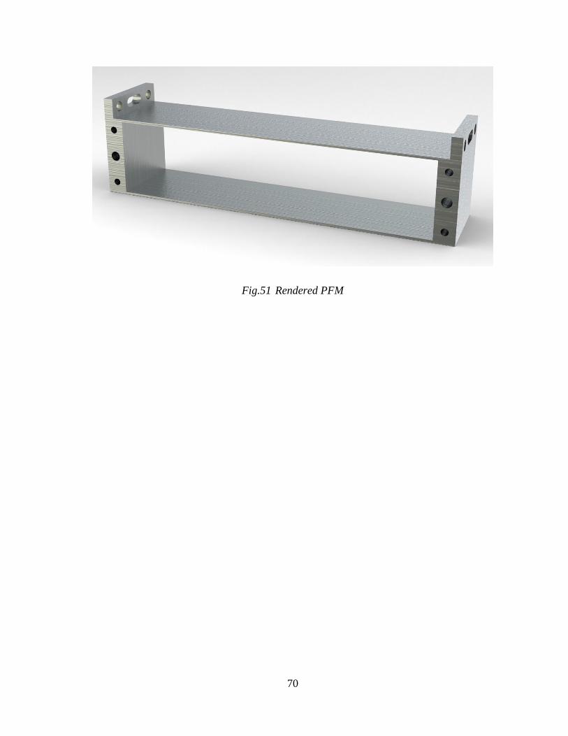
70

Fig.51 Rendered PFM

71

APPENDIX B

Experimental Procedure

Before All Tests

1. Mount Encoders

a. Strips

i. Align with the two dowels.

ii. Attach datum clamps using metal spacer, then tighten.

iii. Attach tension clamp with spacer.

iv. Make sure that the strip is against both dowels and that the clamps do not

touch the sides of the strip.

b. Readhead

i. Attach to mounts using two M3 screws.

ii. Align so that the indicator turns green and tighten the screws. You may

need to use shims to get good alignment. This does not need to be perfect

because the encoders will be fine-tuned once the actuators are mounted.

2. Mount Load Cell

a. Screw the load cell into the X Stage decoupler. Make sure that it sits flush.

3. Mount Actuators

a. X Stage DC Mike

i. Screw the load cell adapter into the end of the DC Mike.

ii. Screw the DC Mike into the load cell until it is connected. Do not tighten

too much because the load cell is delicate.

iii. Make sure the DC Mike is about halfway in its range. If it not, carefully

apply voltage to get it there.

iv. Tighten the DC Mike into the X actuator mount.

v. To make sure the X stage is at its neutral position:

1. Run the DSpace program to view the output of the cap probes.

2. Move the X actuator (by commanding small positions) until the

cap probe reading show a minimum displacement. This is the X

zero position.

b. Y and Z Stage DC Mikes (or dummy actuators)

i. Mount the actuators to the decoupler adapters.

ii. If using DC Mikes, adjust the position until it is in the middle of its range.

iii. To make sure the Y and Z stages are in their neutral positions

1. Hold a gage block (preferably 4 inches long) against the

appropriate flexure.

72

2. Adjust the actuator until no gap can be seen between the gage

block and the flexure. This is the zero position.

Sensor Setup 1 (Cap probes in Z Axis of X Stage)

This setup measures the actuation force and Z translation of the X stage against X actuation

for various Y and Z actuations.

4. Mount Cap Probes

a. Using super glue, carefully (and quickly) attach the ground aluminum plate to the

side of the X Stage. First clean the two surfaces with acetone to remove any

residual glue. Use only two drops of glue on the X stage, making sure to avoid

the dowel and screw holes. Hold the plate firmly against the stage, checking that it

is flush.

b. Tighten the mount to the ground.

c. Insert the three C1-A cap probes. Facing the negative Z direction, the top left is

CP1, the top right is CP2, and the bottom left is CP3.

d. Make sure all three probes are in “high-sensitivity” mode. Adjust each probe until

the indicator LED reads one unit above “near”, and then tighten the screws. This

is because the stage is expected to only move further away with all inputs.

5. Run the tests

a. For each test, Y and Z are held at a fixed position while X is cycled using a

controller from 0 to +3mm to 0 to -3mm to 0 in 1mm increments. Each transition

is a 1 second ramp, and each position is held constant for 10 seconds. The total

test time is 145 seconds.

b. For the first test (Y = 0, Z = 0)

i. Align the encoders

1. Connect the encoders to the PC using the USB output.

2. Run the Signum Software to view the signal strength and pitch of

the readhead.

3. Adjust each readhead until the signal is close to 100% and the

pitch is level. Note: the signal can read 100% even if the pitch is

not level. This can cause bad results as the encoders will lose

signal more rapidly to small changes. Always make sure that the

pitch is level.

ii. Zero the load cell.

iii. Zero the cap probes (if desired).

iv. Run the test and save the data.

c. To switch to another Y, Z location

73

i. It is important to run all tests sequentially and record all data while

moving. This is because the encoder outputs are zeroed at the beginning of

each test.

ii. Run the DSpace program with the X command sequence turned off.

iii. Adjust the Y, Z locations to the next step (e.g. move Z from 0mm to

+2.5mm).

iv. Adjust the X location manually to find its natural zero (this can shift

between tests because the controller doesn’t always return exactly to zero).

v. Wait for the outputs to settle for about 10 seconds.

vi. Stop the program and save.

d. Run the next test

i. Align the encoders

1. Connect the encoders to the PC using the USB output.

2. Run the Signum Software to view the signal strength and pitch of

the readhead.

3. Adjust each readhead until the signal is close to 100% and the

pitch is level. Note: the signal can read 100% even if the pitch is

not level. This can cause bad results as the encoders will lose

signal more rapidly to small changes. Always make sure that the

pitch is level.

ii. Do NOT zero the load cell or cap probes.

iii. Run the test with the X command sequence turned on and save the data,

keeping an eye on the encoder signal strength.

Sensor Setup 2 (Cap probes in Y Axis of X Stage)

This setup measures the Y translation of the X stage against Y actuation for various Z

actuations.

1. Mount the cap probes

a. Tighten the mount to the ground.

b. Insert two C1-A cap probes. Facing the negative Z direction, the left is CP1

and the right is CP2.

c. One additional C1-A cap probe can be mounted along the Z axis of the X

stage to measure the zero location of the X stage.

d. Make sure all three probes are in “high-sensitivity” mode. Adjust each probe

until the indicator LED is in the middle, and then tighten the screws.

2. Run the tests

a. For each test, X is held at 0, Y is fixed, and Z is cycled either manually or

using a controller from 0 to +3mm to 0 to -3mm to 0 in 1mm increments.

74

Each transition is a 1 second ramp, and each position is held constant for 10

seconds. The total test time is 145 seconds.

b. For the first test (X = 0, Y = 0)

i. Align the encoders

1. Connect the encoders to the PC using the USB output.

2. Run the Signum Software to view the signal strength and pitch

of the readhead.

3. Adjust each readhead until the signal is close to 100% and the

pitch is level. Note: the signal can read 100% even if the pitch

is not level. This can cause bad results as the encoders will lose

signal more rapidly to small changes. Always make sure that

the pitch is level.

ii. Zero the load cell.

iii. Zero the cap probes (if desired).

iv. Run the test and save the data.

c. To switch to another Y location

i. It is important to run all tests sequentially and record all data while

moving. This is because the encoder outputs are zeroed at the

beginning of each test.

ii. Run the DSpace program with the X command sequence turned off.

iii. Adjust the Y location to the next step (e.g. move Y from 0mm to

+2.5mm).

iv. Wait for the outputs to settle for about 10 seconds.

v. Stop the program and save.

d. Run the next test

i. Align the encoders

1. Connect the encoders to the PC using the USB output.

2. Run the Signum Software to view the signal strength and pitch

of the readhead.

3. Adjust each readhead until the signal is close to 100% and the

pitch is level. Note: the signal can read 100% even if the pitch

is not level. This can cause bad results as the encoders will lose

signal more rapidly to small changes. Always make sure that

the pitch is level.

ii. Do NOT zero the load cell or cap probes.

iii. Run the test with the Z command sequence turned on and save the

data, keeping an eye on the encoder signal strength.

75

Sensor Setup 3 (Cap probes in Z Axis of XYZ Stage)

This setup measures the X rotation of the XYZ stage against Y actuation for various Z

actuations.

1. Mount the cap probes

a. Using super glue, carefully (and quickly) attach the ground aluminum plate to

the XY plane of the XYZ Stage. First clean the two surfaces with acetone to

remove any residual glue. Use only two drops of glue on the XYZ stage,

making sure to avoid the dowel and screw holes. Hold the plate firmly against

the stage, checking that it is flush.

b. Tighten the mount to the ground.

c. Insert the three C1-A cap probes. Facing the negative Z direction, the top left

is CP1, the top right is CP2, and the bottom right is CP3.

d. Make sure all three probes are in “low-sensitivity” mode. Adjust each probe

until the indicator LED is in the middle, and then tighten the screws.

2. Run the tests

a. For each test, X is held at 0, Z is fixed, and Y is cycled either manually or

using a controller from 0 to +3mm to 0 to -3mm to 0 in 1mm increments.

Each transition is a 1 second ramp, and each position is held constant for 10

seconds. The total test time is 145 seconds.

b. For the first test (X = 0, Z = 0)

i. Align the encoders

1. Connect the encoders to the PC using the USB output.

2. Run the Signum Software to view the signal strength and pitch

of the readhead.

3. Adjust each readhead until the signal is close to 100% and the

pitch is level. Note: the signal can read 100% even if the pitch

is not level. This can cause bad results as the encoders will lose

signal more rapidly to small changes. Always make sure that

the pitch is level.

ii. Zero the load cell.

iii. Zero the cap probes (if desired).

iv. Run the test and save the data.

c. To switch to another Y location

i. It is important to run all tests sequentially and record all data while

moving. This is because the encoder outputs are zeroed at the

beginning of each test.

ii. Run the DSpace program with the Y command sequence turned off.

76

iii. Adjust the Y location to the next step (e.g. move Z from 0mm to

+2.5mm).

iv. Wait for the outputs to settle for about 10 seconds.

v. Stop the program and save.

d. Run the next test

i. Align the encoders

1. Connect the encoders to the PC using the USB output.

2. Run the Signum Software to view the signal strength and pitch

of the readhead.

3. Adjust each readhead until the signal is close to 100% and the

pitch is level. Note: the signal can read 100% even if the pitch

is not level. This can cause bad results as the encoders will lose

signal more rapidly to small changes. Always make sure that

the pitch is level.

ii. Do NOT zero the load cell or cap probes.

iii. Run the test with the Y command sequence turned on and save the

data, keeping an eye on the encoder signal strength.

Sensor Setup 4 (Cap probes in Z Axis of XYZ Stage)

This setup measures the X direction lost motion against X and Y actuations with Z fixed at 0.

1. Mount the cap probes

a. Using super glue, carefully (and quickly) attach the ground aluminum plate to

the YZ plane of the XYZ Stage. First clean the two surfaces with acetone to

remove any residual glue. Use only two drops of glue on the XYZ stage,

making sure to avoid the dowel and screw holes. Hold the plate firmly against

the stage, checking that it is flush.

b. Tighten the mount to the ground.

c. Insert the three C1-A cap probes. Facing the negative X direction, the top left

is CP1, the top right is CP2, and the bottom right is CP3.

d. Make sure all three probes are in “low-sensitivity” mode. Adjust each probe

until the indicator LED is in the middle, and then tighten the screws.

2. Run the tests

a. For each test, Z is held at 0, and either X or Y is fixed while the other is

cycled either manually or using a controller from 0 to +3mm to 0 to -3mm to

0 in 1mm increments. Each transition is a 1 second ramp, and each position is

held constant for 10 seconds. The total test time is 145 seconds.

b. For the first test (Z = 0, Y = 0)

i. Align the encoders

77

1. Connect the encoders to the PC using the USB output.

2. Run the Signum Software to view the signal strength and pitch

of the readhead.

3. Adjust each readhead until the signal is close to 100% and the

pitch is level. Note: the signal can read 100% even if the pitch

is not level. This can cause bad results as the encoders will lose

signal more rapidly to small changes. Always make sure that

the pitch is level.

ii. Zero the load cell.

iii. Zero the cap probes (if desired).

iv. Run the test and save the data.

c. To switch to another Y location

i. It is important to run all tests sequentially and record all data while

moving. This is because the encoder outputs are zeroed at the

beginning of each test.

ii. Run the DSpace program with the X command sequence turned off.

iii. Adjust the Y location to the next step (e.g. move Z from 0mm to

+2.5mm).

iv. Wait for the outputs to settle for about 10 seconds.

v. Stop the program and save.

d. Run the next test

i. Align the encoders

1. Connect the encoders to the PC using the USB output.

2. Run the Signum Software to view the signal strength and pitch

of the readhead.

3. Adjust each readhead until the signal is close to 100% and the

pitch is level. Note: the signal can read 100% even if the pitch

is not level. This can cause bad results as the encoders will lose

signal more rapidly to small changes. Always make sure that

the pitch is level.

ii. Do NOT zero the load cell or cap probes.

iii. Run the test with the X command sequence turned on and save the

data, keeping an eye on the encoder signal strength.

Note: If the encoders become misaligned too much, the output will stray from actual. If the X

encoder strays, the test will need to be rerun. As another check, rerun the first test at the end

and look for drift in either the load cell or the cap probes. If the drift is significant, all of the

tests will need to be rerun.

78

REFERENCES

[1] Jones, R. V., 1962, "Some uses of elasticity in instrument design," Journal of Scientific

Instruments, (39), pp.193-203

[2] Smith, S. T., 2000, Flexures: Elements of Elastic Mechanisms, Gordon and Breach

Science Publishers

[3] Slocum, A. H., 1992, Precision Machine Design, Society of Manufacturing Engineers,

Dearborn, MI

[4] Awtar, S., Ustick, J., and Sen, S., 2011, "An XYZ Parallel Kinematic Flexure Mechanism

with Geometrically Decoupled Degrees of Freedom," Proc. ASME IDETC/CIE,

Washington DC, Paper # 47713

[5] Fischer, F. L., 1981, Symmetrical 3 DOF Compliance Structure, US Patent 4,447,048

[6] Bednorz, J. G., Hollis Jr., R. L., Lanz, M., Pohl, W. D., and Yeack-Scranton, C. E., 1985,

Piezoelectric XY Positioner, 4,520,570

[7] Davies, P. A., 2001, Positioning Mechanism, US 6,193,226

[8] Dagalakis, N. G., and Amatucci, E., 2001, "Kinematic Modeling of a 6 Degree of

Freedom Tri-Stage Micro-Positioner," Proc. ASPE 16th Annual Meeting, Crystal City

VA

[9] Yao, Q., Dong, J., and Ferreira, P. M., 2008, "A novel parallel-kinematics mechanisms

for integrated, multi-axis nanopositioning. Part 1. Kinematics and design for fabrication,"

Precision Engineering, 32(1), pp.7-19

[10] Hicks, T. R., and Atherton, P. D., 1997, The Nanopositioning Book, Queensgate

Instruments Ltd.

[11] Application Note: Nanopositioning Tools and Techniques for R&D Applications, nPoint

Inc.

[12] Jordan, S., and Lula, B., 2005, "Nanopositioning: The Technology and the Options,"

The 2005 Photonics Handbook

[13] Dai, G., Pohlenz, F., Danzebrink, H.-U., Xu, M., Hasche, K., and Wilkening, G., 2004,

"Metrological large range scanning probe microscope," Review of Scientific Instruments,

75(4), pp.962-969

[14] Sinno, A., Ruaux, P., Chassagne, L., Topcu, S., and Alayli, Y., 2007, "Enlarged Atomic

Force Microscopy Scanning Scope: Novel Sample-holder Device with Millimeter

Range," Review of Scientific Instruments, 78(9), pp.1-7

[15] Wouters, D., and Schubert, U. S., 2004, "Nanolithography and nanochemistry: Probe-

related patterning techniques and chemical modification for nanometer-sized devices,"

Angewandte Chemie International Edition, 43(19), pp.2480–2495

[16] Beeby, S., Tudor, M., and White, N., 2006, "Energy harvesting vibration sources for

microsystems applications," Measurement Science and Technology, (12), pp.R175-R195

[17] Mitcheson, P. D., Rao, G. K., and Green, T. C., 2008, "Energy Harvesting From Human

and Machine Motion for Wireless Electronic Devices," Proc. IEEE, 96(9), pp.1457-1486

[18] Smith, S. T., and Seugling, R. M., 2006, "Sensor and actuator considerations for

precision, small machines," Precision Engineering, 30(3), pp. 245-264

[19] Awtar, S., and Slocum, A. H., 2007, "Constraint-based Design of Parallel Kinematic XY

Flexure Mechanisms," ASME Journal of Mechanical Design, 129(8), pp.816-830

[20] Blanding, D. L., 1999, Exact Constraint: Machine Design Using Kinematic Principles,

ASME Press, New York

79

[21] Hopkins, J. B., and Culpepper, M. L., 2010, "Synthesis of multi-degree of freedom,

parallel flexure system concepts via Freedom and Constraint Topology (FACT) - Part I:

Principles," Precision Engineering, 34(2), pp.259-270

[22] Su, H.-J., and Tari, H., 2010, "Realizing orthogonal motions with wire flexures

connected in parallel," ASME Journal of Mechanical Design, 132(12)

[23] Awtar, S., Shimotsu, K., and Sen, S., 2010, "Elastic Averaging in Flexure Mechanisms:

A Three-Beam Parallelogram Flexure Case Study," Journal of Mechanisms and Robotics,

2(4)

[24] Culpepper, M. L., and Anderson, G., 2004, "Design of a low-cost nano-manipulator

which utilizes a monolithic, spatial compliant mechanism," Precision Engineering, 28(4),

pp.469-482

[25] Yamakawa, K., Furutani, K., and Mohri, N., 1999, "XYZ-stage for Scanning Probe

Microscope by Using Parallel Mechanism," Proc. ASME DETC

[26] Li, Y., and Xu, Q., 2005, "Kinematic Design of a Novel 3-DOF Compliant Parallel

Manipulator for Nanomanipulation," Proc. 2005 IEEE/ASME International Conference

on Advanced Intelligent Mechatronics, Monterey, CA

[27] Arai, T., Herve, J. M., and Tanikawa, T., 1996, "Development of 3 DOF micro finger,"

Proc. Intelligent Robots and Systems '96

[28] Xueyen, T., and Chen, I. M., 2006, "A Large-Displacement and Decoupled XYZ

Flexure Parallel Mechanism for Micromanipulation," Proc. IEEE International

Conference on Automation Science and Engineering

[29] Hao, G., and Kong, X., 2009, "A 3-DOF Translational Compliant Parallel Manipulator

Based on Flexure Motion," Proc. ASME IDETC, Paper # 49040

[30] Li, F., Wu, M. C., Choquette, K. D., and Crawford, M. H., 1997, "Self-assembled

microactuated XYZ stages for optical scanning and alignment," Proc. TRANSDUCERS

'97, Chicago

[31] Ando, Y., 2004, "Development of three-dimensional electrostatic stages for scanning

probe microscope," Sensors and Actuators A: Physical, 114(2-3), pp.285-291

[32] Mcneil, A. C., Li, G., and Koury, D. N., 2005, Single Proof Mass 3 Axis MEMS

Transducer, US 6,936,492

[33] Xinyu, L., Kim, K., and Sun, Y., 2007, "A MEMS stage for 3-axis nanopositioning,"

Journal of Micromechanics and Microengineering, 17(9)

[34] Sarkar, N., Geisberger, A., and Ellis, M. D., 2004, Fully Released MEMS XYZ Flexure

Stage with Integrated Capacitive Feedback, US Patent 6,806,991

[35] XYZ Flexure Demonstration Video, http://www-

personal.umich.edu/~awtar/XYZ%20flexure%20video1.mp4

[36] Awtar, S., Slocum, A. H., and Sevincer, E., 2007, "Characteristics of Beam-based

Flexure Modules," ASME Journal of Mechanical Design, 129(6), pp.625-639

[37] Awtar, S., and Parmar, G.., 2010,"Design of a Large Range XY Nanopositioning

System", Proc. IDETC/CIE 2010, Montreal, Canada, Paper No. 28185

[38] Awtar, S., 2011, Multiple Degrees of Freedom Motion System, US 8,072,120

[39] Chen, K. S., Trumper, D. L., and Smith, S. T., 2002, "Design and control for an

electromagnetically driven X-Y- stage," Precision Engineering, 26(4)

[40] Siddall, G. J., 1987, Flexure Stage Alignment Apparatus, US 4,694,477

80

[41] Awtar, S., Trutna, T. T., Nielsen, J. M., Abani, R., and Geiger, J. D., 2010, "FlexDex: A

Minimally Invasive Surgical Tool with Enhanced Dexterity and Intuitive Actuation,"

ASME Journal of Medical Devices, 4(3)

[42] Du, E., Cui, H., and Zhu, Z., 2006, "Review of nanomanipulators for

nanomanufacturing," International Journal of Nanomanufacturing, 1(1)

[43] Howell, L. L., 2001, Compliant Mechanisms, John Wiley & Sons

[44] Awtar, S., Slocum, A.H., and Sevincer E., 2007, "Characteristics of Beam-based Flexure

Modules", ASME Journal of Mechanical Design, 129 (6), pp. 625-639

[45] Dai, G., Pohlenz, F., Danzebrink, H.-U., Xu, M., Hasche, K., and Wilkening, G., 2004,

"Metrological large range scanning probe microscope," Review of Scientific Instruments,

75(4), pp. 962-969.

[46] Hausotte, T., Jaeger, G., Manske, E., Hofmann, N., and Dorozhovets, N., 2005,

"Application of a Positioning and Measuring Machine for Metrological Long-range

Scanning Force Microscopy," Proc. SPIE, San Diego, CA, 5878(2), pp. 1-12.

[47] Sinno, A., Ruaux, P., Chassagne, L., Topcu, S., and Alayli, Y., 2007, "Enlarged Atomic

Force Microscopy Scanning Scope: Novel Sample-holder Device with Millimeter

Range," Review of Scientific Instruments, 78(9), pp. 1-7.

[48] Weckenmann, A., and Hoffmann, J., 2007, "Long Range 3D Scanning Tunneling

Microscopy," CIRP Annals - Manufacturing Technology, 56(1), pp. 525-528.

[49] Salaita, K., Wang, Y. H., and Mirkin, C. A., 2007, "Applications of Dip-Pen

Nanolithography," Nature Nanotechnology, 2(3), pp. 145-55.

[50] O'brien, W., 2005, "Long-range motion with nanometer precision," Photonics Spectra,

39

[51] Zhu, D., & Beeby, S. (2011). “Chapter 1: Kinetic Energy Harvesting,” Energy

Harvesting Systems: Principles, Modeling and Applications, pp. 1-14.

[52] Hopkins, J. B., and Culpepper, M. L., 2010, "Synthesis of multi-degree of freedom,

parallel flexure system concepts via Freedom and Constraint Topology (FACT) - Part III:

Numerations and Type Synthesis of Flexure Mechanisms," Precision Engineering.

[53] Huang Z., and Li Q.C. 2003, “Type synthesis of symmetrical lower-mobility parallel

mechanisms using the constraint synthesis method”. International Journal of Robotics

Research, 22(1): 59-79.

[54] Fang Y.F., and Tsai L.W. 2002, “Structure synthesis of a class of 4-DoF and 5-DoF

parallel manipulators with identical limb structures”. International Journal of Robotics

Research, 21(9): 799-810.