Design flood elevations beyond code requirements and

Louisiana State UniversityLSU Digital Commons

LSU Master's Theses Graduate School

2013

Design flood elevations beyond code requirementsand current best practicesFrank H. BohnLouisiana State University and Agricultural and Mechanical College

Follow this and additional works at: https://digitalcommons.lsu.edu/gradschool_theses

Part of the Engineering Science and Materials Commons

This Thesis is brought to you for free and open access by the Graduate School at LSU Digital Commons. It has been accepted for inclusion in LSUMaster's Theses by an authorized graduate school editor of LSU Digital Commons. For more information, please contact [email protected].

Recommended CitationBohn, Frank H., "Design flood elevations beyond code requirements and current best practices" (2013). LSU Master's Theses. 69.https://digitalcommons.lsu.edu/gradschool_theses/69

https://digitalcommons.lsu.edu?utm_source=digitalcommons.lsu.edu%2Fgradschool_theses%2F69&utm_medium=PDF&utm_campaign=PDFCoverPages

https://digitalcommons.lsu.edu/gradschool_theses?utm_source=digitalcommons.lsu.edu%2Fgradschool_theses%2F69&utm_medium=PDF&utm_campaign=PDFCoverPages

https://digitalcommons.lsu.edu/gradschool?utm_source=digitalcommons.lsu.edu%2Fgradschool_theses%2F69&utm_medium=PDF&utm_campaign=PDFCoverPages

https://digitalcommons.lsu.edu/gradschool_theses?utm_source=digitalcommons.lsu.edu%2Fgradschool_theses%2F69&utm_medium=PDF&utm_campaign=PDFCoverPages

http://network.bepress.com/hgg/discipline/279?utm_source=digitalcommons.lsu.edu%2Fgradschool_theses%2F69&utm_medium=PDF&utm_campaign=PDFCoverPages

https://digitalcommons.lsu.edu/gradschool_theses/69?utm_source=digitalcommons.lsu.edu%2Fgradschool_theses%2F69&utm_medium=PDF&utm_campaign=PDFCoverPages

mailto:[email protected]

DESIGN FLOOD ELEVATIONS BEYOND CODE REQUIREMENTS AND CURRENT BEST PRACTICES

A Thesis

Submitted to the Graduate Faculty of the Louisiana State University and

Agricultural and Mechanical College in partial fulfillment of the

requirements for the degree of Master of Science

in

Engineering Science

by Frank Bohn

B.S., Louisiana State University, 2012 May 2013

i

To my hardworking & supporting professors

&

To my fellow co-workers

&

To my family and friends

&

To those affected by storm surge and hurricanes

&

To all those aided by the results of this research

ii

ACKNOWLEDGEMENTS

I would like to thank my committee members Dr. Dean Adrian, Dr. Carol Friedland &

Dr. Emerald Roider. I would like to sincerely thank Dr. Carol Friedland for her guidance and

recommending the Masters of Engineering Science when I was in search of a minor. Dr.

Friedland recommended this research topic to me having been aware of my family’s past flood

losses due to Hurricane Ike. I would also like to thank Dr. Friedland for being patient with me

during my times of slow progress.

I am thankful for LSU’s Coastal Sustainability Studio providing funding for my first year

of research. I would also like to acknowledge Carol Massarra, Hal Needham, and Ahmet

Binselam for providing immediate feedback on requests for information countless times.

Most importantly, I would like to thank my parents and family for providing me the

opportunity to attend such a wonderful university and continuing my education beyond my

Bachelor’s degree. They expressed the importance and value of obtaining a good education and

giving it your very best while reminding me if it was easy, everybody would do it. I would also

like to thank my girlfriend Krista who always helped me resolve issues and kept me calm when I

was simply too frustrated to think straight.

iii

TABLE OF CONTENTS

ACKNOWLEDGEMENTS ........................................................................................................... iii

LIST OF TABLES ......................................................................................................................... vi

LIST OF FIGURES ...................................................................................................................... vii

ABSTRACT ................................................................................................................................. viii

CHAPTER 1: INTRODUCTION .................................................................................................1 1.1 Problem Statement ......................................................................................................5 1.2 Goals and Objectives ..................................................................................................5 1.3 Scope of Study ............................................................................................................6 1.4 Limitations of Study ...................................................................................................7 1.5 Organization of the Thesis ..........................................................................................8 1.6 Definitions...................................................................................................................8

CHAPTER 2: A Comprehensive Method to Determine Design Flood Elevations for Structures in Coastal High Hazard Flood Zones .................................................12

2.1 Introduction ...............................................................................................................12 2.2 Current Code and Best Practices Literature ..............................................................14 2.3 Gaps in Current Code and Practices .........................................................................17

2.3.1 Datum Conversions ....................................................................................17 2.3.2 Global Sea Level Rise ................................................................................19 2.3.3 Consideration of Tides ...............................................................................21 2.3.4 Flood Return Intervals ................................................................................25

2.4 Proposed Design Practices ........................................................................................26 2.4.1 Datum Conversion......................................................................................28 2.4.2 Effects of GSLR .........................................................................................29 2.4.3 Tidal Influence ...........................................................................................30 2.4.4 Determine Lowest Eroded Ground Elevation (GS) and Erosion Effects ...31 2.4.5 Find the Design Stillwater Depth, ds. .........................................................32 2.4.6 Maximum Wave Crest ...............................................................................32 2.4.7 Design Flood Elevation ..............................................................................32

2.5 Summary of Code, Code-Plus and Recommended Practices ...................................33 2.6 Case Study ................................................................................................................33 2.7 Conclusion ................................................................................................................37 2.8 Acknowledgements ...................................................................................................39

CHAPTER 3: Estimating Coastal Flood Elevations for Return periods Exceeding Current NFIP Guidance Using Existing FIS ....................................................................40

3.1 Introduction ...............................................................................................................40 3.1.1 Background on NFIP and the 100-year flood ............................................42 3.1.2 Probability of Exceedance ..........................................................................45 3.1.3 Return Periods and Annual Maxima ..........................................................45 3.1.4 Current Coastal Flood Design Practices.....................................................47

3.2 Methodology .............................................................................................................49

iv

3.2.1 Data Collection ...........................................................................................49 3.2.2 Data Compilation .......................................................................................50 3.2.3 Estimated 500-Year SWEL Values ............................................................52 3.2.4 Estimated 700- and 1700-Year SWEL Values ...........................................55 3.2.5 Normalized Data ........................................................................................57

3.3 Conclusion and Recommendations ...........................................................................59

CHAPTER 4: Conclusions and Recommendations ....................................................................61 4.1 Introduction ...............................................................................................................61

4.1.1 Summary ....................................................................................................61 4.2 Framework for New Recommendations ...................................................................65 4.3 Conclusions and Applications ...................................................................................65 4.4 Final Remarks ...........................................................................................................67

REFERENCES ..............................................................................................................................70

APPENDIX A: SUMMARY OF TRANSECT SELECTION.......................................................75

APPENDIX B: REGRESSION PLOTS FOR EACH COMMUNITY .........................................78

VITA ..............................................................................................................................................83

v

LIST OF TABLES

Table 1.1 Definitions and Variables Used to Describe Coastal Flood Hazards, Building Elevation Design, and the NFIP................................................................8

Table 2.1 CCM Building Elevation Options ..........................................................................16

Table 2.2 Code, Best Practices, and Recommended Practices Summary ..............................34

Table 3.1 Probability of Exceedance for Events During Expected Useful Life (Friedland and Gall 2012) ......................................................................................45

Table 3.2 Summary of ASCE 24 Elevation Requirements for Lowest Horizontal Structural Member (ASCE 2005) ..........................................................................48

Table 3.3 Summary of Selected Flood Insurance Studies .....................................................51

Table 3.4 Average FIS Transect Data by Recurrence Interval (ft) ........................................51

Table 3.5 Differences Between Projected 500-year SWEL and FIS SWEL .........................53

Table 3.6 Differences Between the Regressed 500-year SWEL Values and the FIS 500-year SWEL .....................................................................................................54

Table 3.7 Summary of SRCC and Huff-Angel Regression Equations and R2-Values ..........56

Table 3.8 Summary of Information used to Extrapolate 700 and 1700-year SWEL Values ....................................................................................................................56

Table 3.9 Generalized 700- and 1700-Year Estimate Guidelines - 95% Confidence Interval ...................................................................................................................59

vi

LIST OF FIGURES

Figure 2.1 ASCE 24 DFE Determination Process ..................................................................16

Figure 2.2 Tidal Gauge Data Collected by NOAA Co-Ops Buoys During Hurricanes (A) 2004 Ivan, (B) 2008 Ike, and (C) 2012 Isaac .................................................23

Figure 2.3 Percentages of the Maximum Surge Elevation Shown as a Percentage of a 24-hour Day. ..........................................................................................................24

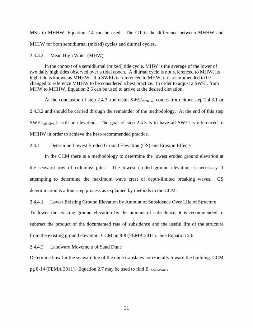
Figure 2.4 Case Study – St. Johns County, Florida .................................................................35

Figure 3.1 Extreme SWEL Values Normalized About the 100-year SWEL ..........................58

vii

ABSTRACT

In the United States, nearly 9 million people, 3.0% of the population, live in areas subject

to the 1% annual chance (100-yr) coastal flood hazard. New construction and substantial

improvements in coastal high hazard areas require structures to be elevated above the design

flood elevation (DFE), without the use of fill (Bellomo et al. 1999). Building code requirements

for flood elevation are linked to the National Flood Insurance Program (NFIP) insurance

policies, and represent the minimum requirement for building elevation. Current elevation

procedures are limited to the 100-year base flood elevation with minimal guidance beyond the

100-year elevation in many locations, which may be of interest to those designing critical

facilities and buildings with a longer design life (e.g. institutional buildings). Additional code-

plus resources exist to provide best available practices for practitioners; however, gaps still exist

that may lead to lower design elevations than warranted for a particular risk level.

In an effort to provide guidance for practitioners, this thesis presents a methodology to

address existing gaps in combination in the context of current best practices. A short case study

to demonstrate the proposed methodology in comparison to code and best practices is provided.

To provide guidance for longer return period flood events, this thesis uses stillwater elevations

(SWEL) from flood insurance studies (FIS) to extrapolate flood elevations associated with longer

return periods. FIS data are fit using the Huff-Angel and SRCC regression models, resulting in

an equation to be used for extrapolating new flood elevations. The results of are evaluated using

R2 values, differences in projected elevations and known elevations for the same return period,

and normalized data for the 100-year SWELs. The result of this work is not intended to become

integrated into current code or policy regulations in the United States, but rather to provide

generalized guidance to aid practitioners in decision making by consolidating current code, best

practices, and characteristics of the changing coastal environment.

viii

CHAPTER 1: INTRODUCTION

Financial losses attributed to floods in the U.S. total $2.4 billion annually, and more than

75% of all federal disaster declarations are related to flood events (Taggart and van de Lindt

2009; Li and van de Lindt 2012). Improving the practices and methods used for development

within or near floodplains can help to reduce flood-induced losses. In 2000, USGS reported

floods during the 20th century were the number-one hazard in terms of loss of life and financial

damage (USGS 2000). Three of the thirty-two most significant flood events of the 20th century

were a result of hurricane storm surge (Perry 2000). These three events were responsible for

greater loss of life than all the rest of the events combined - the 1900 Galveston Hurricane which

claimed 6,000+ lives, the worst on record; a 1938 unnamed hurricane responsible for 494

fatalities in the northeast U.S.; and 1969 Hurricane Camille causing 259 casualties (Perry 2000).

This report does not include 2005 Hurricane Katrina, where storm surge 28 feet above sea level

claimed 1,700+ lives (FEMA 2006). Coastal buildings are the first line of defense against storm

surge and coastal flooding. As a means to mitigate the drastic economic losses and loss of life

associated with storm surge and coastal flooding events, there is a need to expand our

understanding of factors affecting flood elevations and how building design is affected by such

factors.

The 1%-annual-chance flood is the basis for current standards, as established by the

National Flood Insurance Program (NFIP), which was established through the National Flood

Insurance Act of 1968 (Power and Shows 1979). The 1%-annual-chance represents the flood

level that has a 1% chance of occurring or being exceeded every year. This elevation standard is

used as a means to minimize flood losses by requiring buildings to be elevated at or above a

location-specific base flood elevation (BFE) to prevent water from entering a building. The 1%

annual chance flood is also referred to as the 100-year flood and the “base flood elevation”

1

(BFE). The 100-year flood should not be mistaken as a flood that only occurs once every 100

years, but rather has a 1% chance of being equaled or exceeded annually. The 1% annual chance

flood was identified in December 1968 at a floodplain management guidelines seminar at the

University of Chicago by approximately 50 floodplain management researchers convened by the

U.S. Department of Housing and Urban Development (FEMA and Federal Insurance and

Mitigation Administration 2002; Sheaffer 2004). The 100-year flood design standard was

selected as a compromise between those advocating a 50-year or lesser standard and those

advocating a 500-year flood standard (Krimm 2004). Although this decision defined the 100-

year flood as the regulatory floodplain, it also largely affected engineering and construction

practices in the U.S. by limiting development of risk-based design of the built environment

exposed to flood events. Guidance and practices for determining building elevations beyond

insurance requirements should have been established for those who wish to exceed the

insurance-based NFIP minimum requirements. Unfortunately, the 1% recurrence interval BFE

serves as an arbitrary number tied to NFIP insurance rates rather than conveying the real risk

associated with flood hazards.

There are three main primary methods used in the U.S. to mitigate flood risk: elevating

to the BFE in accordance with community-specific requirements, dry-flood proofing (i.e.

preventing water from entering the structure), and wet-flood proofing (i.e. intentionally preparing

the structure for flooding) (FEMA 2009; FEMA 2011). Wet and dry flood proofing are not

viable options for mitigation in Coastal high hazard areas (i.e. V-zones) because of the

hydrodynamic forces that can be imparted on buildings. Coastal high hazard areas are defined as

areas subject to high velocity wave action on a community’s flood hazard map and that are

subject to a breaking wave height equal to or greater than 3-feet (ASCE 2005; ICC 2009). New

construction and substantial improvements of structures in V-zones must be elevated on piles or

2

piers so the lowest horizontal structural member (LHSM) is above the BFE. Structural fill is also

not allowed within V-zones (Bellomo et al. 1999).

The BFE serves only as a minimum requirement, representing a standard size event in

order to manage flood risk for determining insurance rates, thus treating all communities equally

(FEMA and Federal Insurance and Mitigation Administration 2002). The 100-year flood has a

26% (1 in 4) chance of occurring over the life of a 30-year mortgage (FEMA and Federal

Insurance and Mitigation Administration 2002). Designing for a 700-year event would reduce

this probability to a 4.2% chance of occurring over a 30-year mortgage. ASCE wind

requirements call for structures to be designed to the 300, 700, and 1700 year wind according to

their classification (ASCE 2010), yet flood design practice only requires structures to be built to

the 100-year flood plus any freeboard requirements. Freeboard is defined as additional elevation

between the lowest horizontal structural member and the BFE (FEMA 2011). Local jurisdictions

can determine a community freeboard requirement; however, in lieu of local requirements, code-

required freeboard is the same amount for the entire country. Therefore, a critical structure

required to be built to withstand a 1700-year wind speed is only required to design for the 100-

year flood plus two feet of freeboard (ASCE 2005; ASCE 2010). This represents a drastic gap

between flood design and wind design practices. To design buildings and communities with

known levels of risk, more risk-consistent practices should be employed.

As a result of the requirement to design to the 100-year BFE, for the majority of

communities, there is no guidance for practitioners desiring to elevate above 100-year BFE to a

specified recurrence interval flood. Newer Flood Insurance Studies (FIS) are beginning to

provide 500-year stillwater elevations (SWELs), but for the majority of communities, which do

not have 500-year SWEL values, FEMA recommends calculating the 500-year SWEL as 1.25 of

the 100-year SWEL (FEMA and NAHB Research Center 2010). The rule of 1.25 may

3

significantly over estimate for some locations, thus causing extra costs to the owner, and

significantly underestimate for other locations, causing owners’ risk to be significantly higher

than their perceived rate of risk. Flood elevation design guidance consistent with wind design

requirements and with more reliable accuracy should be readily available for practitioners.

The Coastal Construction Manual (CCM) is currently considered the best flood design

practice available by incorporating subsidence effects, sea level rise, and erosion effects with

code regulations (FEMA 2011; FEMA 2011). Although the CCM is considered a step-up from

code requirements (i.e. code-plus), it also only references the 100-year flood elevation and gaps

remain within the recommended practices. Variables neglected by the CCM include vertical

datum conversions from NGVD 29 to NAVD 88, adjustments for high tide, and accounting for

global sea level rise (GSLR) that occurs from the FIS modeling date until the time construction

begins on the structure. Collecting information about flood zones and elevations can be

confusing in and of itself with all of the available sources (e.g. American Society of Civil

Engineers, the International Code Council, FEMA, CCM), yet information on how BFE and

SWEL numbers are determined can be very vague. Aspects of the gap in flood estimation have

been called “wider than desirable” and “difficult to obtain” information on the approaches used

and problems faced with flood design (Pilgrim 1986, 165S-166S). There is a need for a

comprehensive method to estimate the DFE for any annual occurrence probability event that

incorporates code requirements, regulations, best available practices, and new data on the

changing coastal environment.

In the United States, nearly 9 million people (3.0% of the population) live in areas subject

to the 1% annual chance coastal flood hazard (Crowell et al. 2010). A 1997 study found that

there were over 6 million residential structures in Special Flood Hazard Areas (FEMA and

Federal Insurance and Mitigation Administration 2002), a number which has likely increased in

4

the past 15 years as more development occurs in these areas. A better understanding of factors

affecting floods and further elevation guidance can significantly decrease the risk for these 6

million structures and 9 million people. The NFIP indicates $1 billion in flood damages are

avoided annually and structures built to NFIP criteria experience 80% less damage due to

reduced occurrences and severity of losses (FEMA and Federal Insurance and Mitigation

Administration 2002). Thus, guidance beyond NFIP minimums will serve to further decrease

flood damage and create more flood resilient communities.

1.1 Problem Statement

Flood design practitioners are generally limited to information pertaining to the 100-year

BFE. Flood code and wind code are not risk consistent with respect to the return period of each

hazard’s design event, thus lacking uniformity throughout the design process. Code-plus

methodologies are available to help practitioners consider the effects of the changing coastal

environment, but neglect certain aspects of the DFE process. FEMA provides rule of thumb

guidance to estimate the 500-year SWEL, but does not provide guidance to estimate other, longer

return period flood elevations. While recent literature (e.g. CCM) provides guidance beyond

flood insurance rate map (FIRM) BFEs, the practitioner is severely limited in determining any

DFE beyond the 100-year BFE.

1.2 Goals and Objectives

Mitigation and adaptation techniques for flooding in coastal high hazard (V-Zones) is

currently limited to elevating structures (Bellomo et al. 1999). Therefore, the goals of this thesis

are to improve the understanding of coastal flooding in the changing environment and to provide

guidance to practitioners to consider increased mitigation and adaptation for buildings designed

in the coastal environment. As a step toward accomplishment of these goals, the following

objectives are undertaken:

5

• To evaluate current code and code-plus guidance regarding building elevation in coastal high

hazard areas

• To identify existing gaps in code and code-plus practices and to recommend practices to

bridge identified gaps

• To evaluate existing FIS and develop practitioner-oriented guidance for estimating longer

return period flood elevations (e.g. 700 and 1700 years) from existing FIS

1.3 Scope of Study

The DFE methodology presented in Chapter 2 is developed through review and synthesis of

coastal processes, ASCE, IBC, FEMA regulations, and the CCM (code-plus) requirements.

Gaps among these requirements will be noted, and solutions will be presented in the

comprehensive methodology. Chapter 2 should be used by practitioners in flood zones that

experience erosion, global sea level rise (GSLR), subsidence, and whose flood maps are

referenced to NGVD 29. The return period analysis in Chapter 3 will be conducted using FIS

and SWEL data from 16 coastal communities distributed along the U.S. Atlantic and Gulf

Coasts. Guidelines for estimation of longer return period flood elevations will be presented.

ASCE category III & IV structures whose failure could pose a “substantial risk to human life”

and a “substantial economic impact” or “could pose a substantial hazard to the community”

represent critical facilities such as schools serving as shelters, sewage treatment and power

plants, and nuclear hospitals and police stations (ASCE 2005, p. 7; ASCE 2010, p. 2). ASCE

code requires Category III & IV structures to be built to the 1700-year wind, yet the maximum

elevation required by code is the 100-year BFE plus 2-feet of freeboard (ASCE 2005; ASCE

2010).

It is important to note that data are taken from existing FIS and that flood modeling,

historical flood marks, and tidal gage data outside of the FIS are not included in this thesis.

6

Chapter 3 can be used as guidance in initial development phases for critical facilities which

warrant a full probabilistic surge model. Chapter 3 can also be used in communities for schools

and government buildings for a more scientifically based process to determine DFE. The

findings of this thesis are not intended to be used to change code or insurance requirements, but

rather to provide guidance to practitioners wishing to design beyond the 100-year BFE and

include changes occurring in the coastal environment.

1.4 Limitations of Study

The extent of this study is limited to those structures located in coastal high hazard zones.

Chapter 2 is presented as generalized design recommendations; however, implementation of the

methodology requires knowledge of a specific local environment in order to determine effects

caused by local characteristics. If the practitioner’s locale is not in a special flood hazard area,

methodologies for determining wave effects different than presented in Chapter 2 should be used

for more reliable results. FIS SWELs are normally reported as a maximum probability elevation

for an individual coastal transect; therefore, using an elevation from Chapter 3 for an A-Zone

will result in a significantly higher elevation than desired for that given locality. The FIS used

for calculations in Chapter 3 only represent the Gulf Coast and Atlantic Coasts and are separated

by an average of 206 miles with a shortest distance of approximately 90 miles and a maximum

distance of approximately 306 miles between communities. FIS data were limited to those

communities that provided a SWEL for the 10% annual chance (10-year), 2% annual chance (50-

year), 1% annual chance (100-year) and 0.2% annual chance (500-year) events. The results of

Chapter 3 will be more accurate for locations contained within one of the selected FIS. For those

areas between selected FIS communities, assumptions must be made outside of the scope of this

thesis to produce results for the desired location.

7

1.5 Organization of the Thesis

This thesis is organized into two separate manuscript chapters, followed by an overall summary

and conclusions. Chapter 2 relies on combining code requirements, best practices and

developing new recommendations for existing gaps among current methods. Chapter 2 is

intended to provide a single source for code and code-plus practices for flood elevation

information in Special Flood Hazard Areas. Chapter 3 examines the extrapolation of existing

FIS SWELs to estimate flood elevations for the 700 and 1700 year flood in an effort to facilitate

risk-consistent development among flood and wind hazards.

1.6 Definitions

There are many terms and variables that are utilized with respect to coastal flood hazards,

building elevation design, and the NFIP. The flowing definitions (Table 1.1) are provided to

serve as a resource to the reader for use with this thesis.

Table 1.1 Definitions and Variables Used to Describe Coastal Flood Hazards, Building Elevation Design, and the NFIP

Term Definition

Base Flood Elevation (BFE)

Elevation of flooding, including wave height, having a 1% chance of being equaled or exceeded in any given year; minimum NFIP requirement (ASCE 2005).

Coastal A Zone Areas where the stillwater depth of the BFE above the eroded ground elevation is greater than or equal to 1.9 ft, sufficient to support a wave height greater than or equal to 1.5 ft, and where conditions are conducive to the formation and propagation of such waves (ASCE 2005).

Coastal High Hazard Area (Includes V-Zones)

Areas designated as subject to high velocity wave action on a community’s flood hazard map (V-Zones) (ASCE 2005; ICC 2009); or where the SWEL of the BFE above the eroded ground is greater than or equal to 3.8 ft, sufficient of supporting a wave height equal to or greater than 3ft subject to high-velocity wave action or wave-induced erosion; these include V-Zones (ASCE 2005; ICC 2009). Or, an area within a special flood hazard area extending from offshore to the inland limit of a primary frontal dune along an open coast and any other area that is subject to high velocity wave action (ASCE 2005).

8

Table 1.1 Continued

Term Definition

Depth A depth is the measurement from an object to the ground. Depth is not equivalent to elevation.

Design Flood Elevation (DFE)

Elevation of the design flood, including wave height, relative to the datum specified on a community's flood hazard map (ASCE 2005). This only applies to communities that have elected to exceed NFIP requirements; for a community adopting minimum NFIP requirements, the DFE defaults to the BFE (ASCE 2010).

Design flood protection depth (dfp)

The vertical distance between the eroded ground elevation and the DFE. This concept only applies to CCM calculations and it is important to note it is not an elevation.

Design stillwater flood depth (ds)

The vertical distance between the eroded ground elevation (GS) and the stillwater elevation (SWEL) associated with the design flood (FEMA 2011). This concept only applies to CCM calculations and it is important to note it is not an elevation.

Diurnal Tide Cycle One high tide (MHHW) and one low tide (MLLW) per day (U.S. Department of Commerce 2000).

Elevation An elevation within the context of this thesis is a height always referenced to a recognized vertical datum (e.g. NGVD 29 or NAVD 88). Elevation is not equivalent to depth.

Erosion Refers to the wearing or washing away of coastal lands and commonly refers to horizontal recession of the shore (shore erosion) (FEMA 2011). Erosion can also refer to “seabed erosion” which occurs when sediments are transported offshore, resulting in a lowering of the seabed, which increases local water depths and wave heights reaching the shore (FEMA 2011). Both types of erosion are used when determining the erosion effects from the CCM.

Design Stillwater Flood Elevation (ESW)

The design stillwater flood elevation in feet above datum as used in the CCM.

Global (Eustatic) Sea Level Rise (GSLR)

Global sea level, which changes in response to changes in the volume of ocean water and volume ocean basins (Schlumberger 2012). This differs from relative (local) sea level rise, which includes changes in land movement. Global Sea level changes are the same regardless of where measurements are taken (McCue 2010).

Great Diurnal Range (GT)

The difference in height between mean higher high water and lower low water for both the semidiurnal and diurnal cycle (U.S. Department of Commerce 2000)

Lowest Eroded Ground Elevation (GS)

Lowest eroded ground elevation in feet above datum, adjacent to a building, excluding effects of localized scour around the foundation as used in the CCM (FEMA 2011).

9

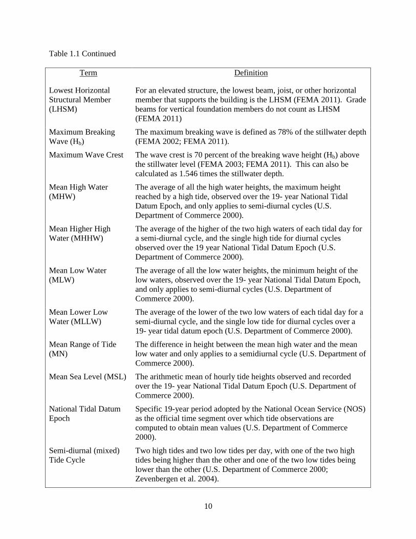
Table 1.1 Continued

Term Definition

Lowest Horizontal Structural Member (LHSM)

For an elevated structure, the lowest beam, joist, or other horizontal member that supports the building is the LHSM (FEMA 2011). Grade beams for vertical foundation members do not count as LHSM (FEMA 2011)

Maximum Breaking Wave (Hb)

The maximum breaking wave is defined as 78% of the stillwater depth (FEMA 2002; FEMA 2011).

Maximum Wave Crest The wave crest is 70 percent of the breaking wave height (Hb) above the stillwater level (FEMA 2003; FEMA 2011). This can also be calculated as 1.546 times the stillwater depth.

Mean High Water (MHW)

The average of all the high water heights, the maximum height reached by a high tide, observed over the 19- year National Tidal Datum Epoch, and only applies to semi-diurnal cycles (U.S. Department of Commerce 2000).

Mean Higher High Water (MHHW)

The average of the higher of the two high waters of each tidal day for a semi-diurnal cycle, and the single high tide for diurnal cycles observed over the 19 year National Tidal Datum Epoch (U.S. Department of Commerce 2000).

Mean Low Water (MLW)

The average of all the low water heights, the minimum height of the low waters, observed over the 19- year National Tidal Datum Epoch, and only applies to semi-diurnal cycles (U.S. Department of Commerce 2000).

Mean Lower Low Water (MLLW)

The average of the lower of the two low waters of each tidal day for a semi-diurnal cycle, and the single low tide for diurnal cycles over a 19- year tidal datum epoch (U.S. Department of Commerce 2000).

Mean Range of Tide (MN)

The difference in height between the mean high water and the mean low water and only applies to a semidiurnal cycle (U.S. Department of Commerce 2000).

Mean Sea Level (MSL) The arithmetic mean of hourly tide heights observed and recorded over the 19- year National Tidal Datum Epoch (U.S. Department of Commerce 2000).

National Tidal Datum Epoch

Specific 19-year period adopted by the National Ocean Service (NOS) as the official time segment over which tide observations are computed to obtain mean values (U.S. Department of Commerce 2000).

Semi-diurnal (mixed) Tide Cycle

Two high tides and two low tides per day, with one of the two high tides being higher than the other and one of the two low tides being lower than the other (U.S. Department of Commerce 2000; Zevenbergen et al. 2004).

10

Table 1.1 Continued

Term Definition

Still Water Elevation (SWEL)

The base water surface elevation upon which the waves ride; it consists of Mean Sea Level (MSL), astronomic tide, and surge (FEMA 2007). Waves are excluded from the SWEL (FEMA 2003); a SWEL is not a depth.

Subsidence Subsidence is a lowering of ground elevation that results from a number of natural and human processes: river diversion and damming preventing re-nourishment of soils (Milliman and Haq 1996); withdrawing large amounts of ground water/petroleum from certain types of rocks (Waller 1982; Milliman and Haq 1996); removal of native vegetation (Zektser et al. 2005); and compaction of the Holocene strata (Tornqvist et al. 2008).

Vertical Datum

A zero elevation coordinate surface and methods of determining heights relative to that surface (Vanicek 1991; National Geodetic Survey 2001). Common National Geodetic Vertical Datum of 1929 (NGVD 29), North American Vertical Datum of 1988 (NAVD 88)

11

CHAPTER 2: A COMPREHENSIVE METHOD TO DETERMINE DESIGN FLOOD ELEVATIONS FOR STRUCTURES IN COASTAL HIGH HAZARD FLOOD ZONES

2.1 Introduction

Financial losses attributed to floods in the U.S. total $2.4 billion annually, and more than

75% of all federal disaster declarations are related to flood events (Taggart and van de Lindt

2009; Li and van de Lindt 2012). Further, nearly 9 million people (3.0% of the U.S. population)

live in areas subject to the 1% annual chance (100-yr) coastal flood hazard (Crowell et al. 2010).

Improving our understanding of coastal flood elevations and the factors affecting these

elevations within the coastal environment can result in improved design and construction

practices that are based on flood risk and probabilities of failure. These practices, if properly

implemented, have potential to reduce flood-induced losses.

The 1% annual chance flood is the basis for current standards, which attempt to minimize

flood losses by requiring buildings to be elevated at or above a base flood elevation to prevent

water from entering a building. Many aspects of the gap in flood estimation are “wider than

desirable” and it is “difficult to obtain” information on the approaches used and problems faced

with flood design (Pilgrim 1986, 165S-166S). In certain situations it may be more cost-effective

to elevate a building above floodwaters than to structurally build to protect against the forces of

floods. There is a need for a revised, comprehensive methodology to determine a more reliable

design flood elevation (DFE) for buildings in coastal communities that is able to be implemented

for any flood recurrence interval.

NFIP Flood Insurance Studies (FIS) and FIRMs do not account for the effects of long-

term erosion, subsidence, or sea level rise, all of which should be considered when establishing

lowest floor elevations in excess of the BFE (FEMA 2011). In addition, for some communities,

the BFE is referenced to an outdated vertical datum (NGVD 29) and the highest of tides are not

12

included in the BFE modeling process. Therefore, the actual risk of flooding is not equivalent to

the intended, or design, risk. All of these long-term effects should be considered in order to

formulate a DFE that addresses the effects of changing coastal characteristics. Flood research

has to date not addressed this issue, and inadequacies in past research have been identified,

specifically in the fundamental decisions underlying design solutions (Pilgrim 1986).

Furthermore, current flood design methods include the addition of “freeboard”, which is defined

as additional elevation between the lowest structural member and the BFE, resulting in the DFE,

which is current basis for design (FEMA 2011). The amount of freeboard is determined by

ASCE standards that are incorporated into the building code or by community adopted freeboard

requirements in excess of the national ASCE standards. Freeboard may be assumed to be largely

arbitrary given that flood elevations for storms of selected recurrence intervals are calculated for

each given locality, yet freeboard required by code is the same amount for the entire country

providing an unknown level of protection.

The Coastal Construction Manual (CCM), currently considered the best practice

available, provides code-plus design recommendations that include long-term effects of

subsidence, sea level rise, and erosion (FEMA 2011; FEMA 2011). However, the CCM does not

account for simultaneous high tides and peak surges, or the total amount of global sea level rise,

and does not explicitly detail vertical datum transformations. The methodology presented in this

chapter builds on the recommendations of the CCM and should be considered and combined

with current best practices available to develop a DFE that will reduce the overall risk of

flooding, thus reducing flood damage from water penetrating the structure. Flood engineering

design and decisions are currently too closely linked with insurance policy decisions. The intent

of this chapter is to provide scientifically based recommendations that focus on the actual risk to

determine a DFE for the desired level of protection.

13

In this chapter, current code and best practices are reviewed and analyzed in the

development of a comprehensive method that addresses current design gaps. The proposed

methodology section introduces the recommended methods combined with current code and

practices to arrive at the proposed DFE. In addition, a case study is provided to show the

implementation of the proposed DFE methodology. The methodology recommended by this

chapter is not intended to apply strictly within the current insurance policy guidelines. That is,

the authors are not making a recommendation about what the National Flood Insurance Program

or other insurers should accept as the required bottom elevation of a building. The purpose of

this chapter is to provide designers with concise additional guidance to develop a building DFE

for a given return interval that integrates all known considerations, codes, and practices.

2.2 Current Code and Best Practices Literature

Current building code requirements in the U.S. integrate International Code Council

(ICC) codes and American Society of Civil Engineers (ASCE) standards. The International

Residential Code (IRC) Section 322.1 General, specifies that, “Buildings and structures located

in whole or in part in identified floodways shall be designed and constructed in accordance with

ASCE 24” (ICC 2009). The International Building Code (IBC) Section 1612.4 Design and

Construction states, “The design and construction of buildings and structures located in flood

hazard areas, including flood hazard areas subject to high-velocity wave action, shall be in

accordance with Chapter 5 of ASCE 7 and with ASCE 24” (ICC 2011).

The standard ASCE 7 Minimum Design Loads for Buildings and Other Structures

provides minimum load requirements for the design of buildings that are subject to code

requirements (ASCE 2010). Chapter 5, Flood Loads, of ASCE 7 presents information for the

design of buildings and structures in areas prone to flooding including erosion and scour; loads

on breakaway walls; hydrostatic loads; hydrodynamic loads; wave loads and breaking wave

14

http://www.madcad.com/library/IBC-09/131347/%23CHAPTER-5

loads on vertical walls; and impact loads from debris (ASCE 2010). ASCE 7 covers flood loads

to be considered when designing, whereas the ASCE 24 Flood Resistant Design and

Construction standard addresses elevation requirements when designing for floods.

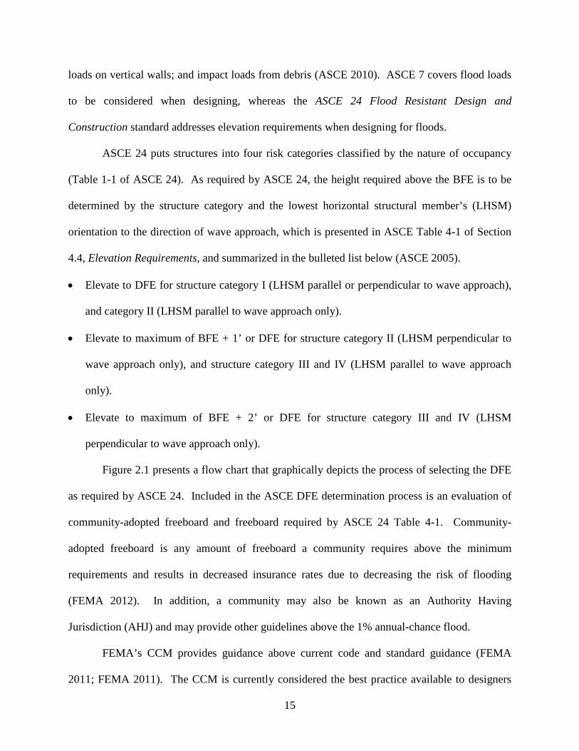
ASCE 24 puts structures into four risk categories classified by the nature of occupancy

(Table 1-1 of ASCE 24). As required by ASCE 24, the height required above the BFE is to be

determined by the structure category and the lowest horizontal structural member’s (LHSM)

orientation to the direction of wave approach, which is presented in ASCE Table 4-1 of Section

4.4, Elevation Requirements, and summarized in the bulleted list below (ASCE 2005).

• Elevate to DFE for structure category I (LHSM parallel or perpendicular to wave approach),

and category II (LHSM parallel to wave approach only).

• Elevate to maximum of BFE + 1’ or DFE for structure category II (LHSM perpendicular to

wave approach only), and structure category III and IV (LHSM parallel to wave approach

only).

• Elevate to maximum of BFE + 2’ or DFE for structure category III and IV (LHSM

perpendicular to wave approach only).

Figure 2.1 presents a flow chart that graphically depicts the process of selecting the DFE

as required by ASCE 24. Included in the ASCE DFE determination process is an evaluation of

community-adopted freeboard and freeboard required by ASCE 24 Table 4-1. Community-

adopted freeboard is any amount of freeboard a community requires above the minimum

requirements and results in decreased insurance rates due to decreasing the risk of flooding

(FEMA 2012). In addition, a community may also be known as an Authority Having

Jurisdiction (AHJ) and may provide other guidelines above the 1% annual-chance flood.

FEMA’s CCM provides guidance above current code and standard guidance (FEMA

2011; FEMA 2011). The CCM is currently considered the best practice available to designers

15

and homebuilders. The CCM was recently revised under the guidance of a technical committee

of national experts, and provides guidance for incorporating the effects of coastal processes that

are not addressed in current codes, standards, or NFIP products. In addition to the FIRM-

specified BFE, which does not consider any long term effects, the CCM provides guidance to

determine the effects of subsidence (if any) on the site, the most landward expected shoreline of

the building over the anticipated life of the building, the lowest expected eroded ground

elevation at the base of the building or structure, and the highest expected stillwater depth at the

building (FEMA 2011). The CCM provides four ways of determining flood protection

elevations (Table 2.1). This chapter considers only Option III, which is the most comprehensive

method by accounting for most factors and future conditions that may increase flood risk.

Figure 2.1 ASCE 24 DFE Determination Process

Table 2.1 CCM Building Elevation Options

Option Description I. 100-year SWEL. Future Conditions not considered.* II. 100-year SWEL plus freeboard. Future conditions not considered.* III. 100-year SWEL. Future Conditions including GSLR and long-term erosion considered for a

specified amount of time.* IV. 500-year wave crest elevation using the AHJ 500-year wave crest. Future conditions not considered. *Options I-III are only ds, the design stillwater flood depth, not an elevation or DFE. In order to arrive at DFE add the ds back to the GS, lowest eroded ground elevation, and then multiply by 1.546 to get to DFE for Coastal High Hazard Zones.

16

2.3 Gaps in Current Code and Practices

Although the CCM increases the level of protection over the ASCE 24 standard, room for

improvement remains. Many of the effective FIS and FIRM elevations, as well as guidance from

the CCM, are referenced to NGVD 29, an older vertical datum currently going out of use. While

using the correct vertical datum is required for a structure’s elevation certificate to be approved,

designers and developers should be provided with better guidance between the available vertical

datums. Neither ASCE nor the CCM provide any such guidance for converting from NAVD 88-

or NGVD 29-referenced elevations. Additionally, the CCM introduces the concept of global sea

level rise (GSLR), but does not account for the total level of GSLR. This total level includes

increases in sea level during the lifetime of the structure in addition to GSLR that occurs prior to

construction. The consideration of high tides should also be included in the design flood

elevation. The effects of storm surge occur over an extended duration and may in fact occur

simultaneously with the highest tide of the day, therefore increasing the risk of flooding. Finally,

FIS have started providing some, yet minimal, information regarding the 500-year flood;

however, most coastal communities still have no guidance for designing above the 100-year

BFE. Return intervals greater than the 100-year BFE should be considered. These gaps are

discussed in further detail in the following sections.

2.3.1 Datum Conversions

A vertical control datum (e.g. NGVD 29 and NAVD 88) is a set of fundamental

elevations to which other elevations are referred (Vanicek 1991; National Geodetic Survey

2001). Many FIS, FIRMs, and CCM recommendations are still referenced to NGVD 29, which

is going out of use, rather than NAVD 88, which is widely accepted nationwide (Iliffe and Lott

2008). NGVD 29 is the National Geodetic Vertical Datum of 1929, also known as the Sea Level

Datum of 1929 until May 10, 1973 (Meyer et al. 2004; National Geodetic Survey 2011).

17

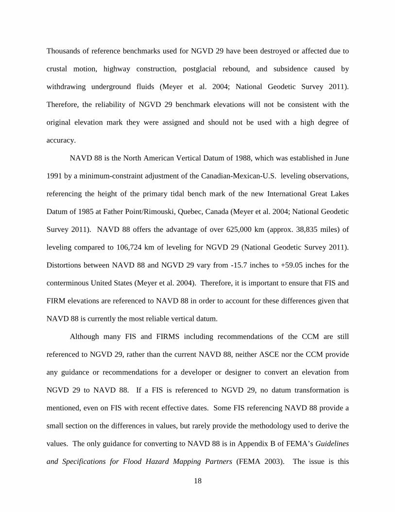
Thousands of reference benchmarks used for NGVD 29 have been destroyed or affected due to

crustal motion, highway construction, postglacial rebound, and subsidence caused by

withdrawing underground fluids (Meyer et al. 2004; National Geodetic Survey 2011).

Therefore, the reliability of NGVD 29 benchmark elevations will not be consistent with the

original elevation mark they were assigned and should not be used with a high degree of

accuracy.

NAVD 88 is the North American Vertical Datum of 1988, which was established in June

1991 by a minimum-constraint adjustment of the Canadian-Mexican-U.S. leveling observations,

referencing the height of the primary tidal bench mark of the new International Great Lakes

Datum of 1985 at Father Point/Rimouski, Quebec, Canada (Meyer et al. 2004; National Geodetic

Survey 2011). NAVD 88 offers the advantage of over 625,000 km (approx. 38,835 miles) of

leveling compared to 106,724 km of leveling for NGVD 29 (National Geodetic Survey 2011).

Distortions between NAVD 88 and NGVD 29 vary from -15.7 inches to +59.05 inches for the

conterminous United States (Meyer et al. 2004). Therefore, it is important to ensure that FIS and

FIRM elevations are referenced to NAVD 88 in order to account for these differences given that

NAVD 88 is currently the most reliable vertical datum.

Although many FIS and FIRMS including recommendations of the CCM are still

referenced to NGVD 29, rather than the current NAVD 88, neither ASCE nor the CCM provide

any guidance or recommendations for a developer or designer to convert an elevation from

NGVD 29 to NAVD 88. If a FIS is referenced to NGVD 29, no datum transformation is

mentioned, even on FIS with recent effective dates. Some FIS referencing NAVD 88 provide a

small section on the differences in values, but rarely provide the methodology used to derive the

values. The only guidance for converting to NAVD 88 is in Appendix B of FEMA’s Guidelines

and Specifications for Flood Hazard Mapping Partners (FEMA 2003). The issue is this

18

information is provided to those developing new flood maps and is not readily available to

designers and practitioners who need to perform a datum conversion for older maps still

referenced to NGVD 29. Although this issue has not been discussed in the literature, the authors

have first-hand observations of practicing engineers, academics, and many others ignoring this

transformation because they are not familiar with the need for datum transformation. It is of

utmost importance to recognize that the correct elevation associated with the correct vertical

datum is required for approval of the elevation certificate. If the elevation certificate is not

approved, then the building will not be permitted for occupancy or use.

One should recognize that not all datum conversions will result in an additive value to the

NGVD 29 elevation, but that some can be subtracted. As an example, at Marco Island in Collier

County, Florida, to arrive at the NAVD 88 elevation, there is a -1.30 foot difference from the

NGVD 29 elevation (FEMA 2009). Many datum transformations in Florida are exceptions

where one might subtract from the NGVD 29 elevation to arrive at the NAVD 88 elevation.

2.3.2 Global Sea Level Rise

While GSLR projections are important for considering future effects, GSLR which has

occurred after the SWEL modeling date but prior to construction is important as well for

determining the total starting SWEL and eventually the DFE. While subsidence affects the

elevation of the structure due to a ‘sinking’ effect, GSLR affects the elevation of the flood by

raising the normal water levels along the coast. By the year 2100, FEMA projects that the area

normally inundated by the 100-year flood (19,500 square miles) will increase to 23,000 square

miles with a 1-foot relative sea level increase and to 27,000 square miles with a 3 foot relative

sea level increase (FEMA and FIA 1991). This is expected to increase the number of households

in the floodplain by 2100 from 2.7 million (as of 1991) to 5.7 million with a 1-foot sea level

increase and 6.8 million with a 3-foot sea level increase (FEMA and FIA 1991). GSLR effects

19

raise the SWEL used in FIRM BFE calculations and the ESW used in CCM calculations (FEMA

2011). An increase to the SWEL and ESW directly increase the maximum wave crest, thus

increasing the risk of a structure to flooding. GSLR raises overall flood levels and increases

flood risk.

The CCM includes the effects of sea level rise over the useful life of the structure, but it

does not account for GSLR that occurs between the effective SWEL modeling date and the start

of construction. When a new FIS is completed, it is not immediately effective, as the adoption

process takes some time, even years. Therefore, it is important to use the modeling date of the

SWEL, as this provides the date that the BFE was computed. If a community publishes a newly

effective FIS with the same SWEL from an older modeling date, then the community has not

accounted for the all effects of GSLR. For example, if an FIS was published in 2010 and uses

the same SWEL that was modeled in 1970, then forty years of GSLR have not been accounted

for. SWELs that remain unchanged from one effective FIS to the next are not uncommon, thus

neglecting changes in sea level over that time period may have considerable effects. GSLR that

has already occurred but is unaccounted for must be considered through the use of recorded

historical GSLR if the modeling date is prior to 1990. For modeling dates after 1990, the

projected annual rate for GSLR assuming a linear distribution of 0.03 feet per year (0.36 inches

per year) is recommended (Rahmstorf 2007; DeMarco et al. 2012).

Future effects of GSLR are included in the CCM and are based on projections. Current

climatological science projects increases in GSLR in the range of 0.5 to 1.4 meters (1.6’ – 4.6’)

from 1990-2100, with 1 meter (3.3’) being the most likely (Rahmstorf 2007; DeMarco et al.

2012). The Louisiana Coastal Protection and Restoration Authority (CPRA) Technical Report

recommends that CPRA staff assume that Gulf sea-level rise will be 1 meter, 3.3’ by 2100, with

a bounding range of 0.5 – 1.5 meters (1.6’ – 4.9’) (DeMarco et al. 2012). A 1-meter increase in

20

sea level will put an additional 14 million people at risk for flooding by 2100, and by 2080, sea

level rise will cause nearly five-times as many people to be flooded than those flooded during a

typical year from storm surge (Nicholls et al. 1999). Failure to acknowledge or account for an

increase in GSLR has the potential to greatly increase design flood damage and underestimate

the risk associated with changing coastal characteristics. Accounting for GSLR is not currently

required by the building code.

2.3.3 Consideration of Tides

Given the long duration of storm surge events, it is very likely that a surge event will

occur simultaneously with a high tide, therefore directly increasing the likelihood of flooding. In

order to provide for maximum protection against flood inundation, the DFE should be referenced

to the highest tide, mean higher high water (MHHW), in the event that a surge event occurs

during high tide. In the event that a DFE is referenced to MSL and peak storm surge occurs

during the highest normal tide of the day (MHHW), the DFE may not accurately account for the

actual risk. According to the USGS, worst-case scenario surge events occur when high tide and

peak storm surge occur concurrently (Perry 2000). It is the assertion of the authors that these are

not truly worst-case scenarios, but rather that they should be anticipated scenarios and included

in the design process.

FEMA’s Guidelines and Specifications for Flood Hazard Mapping Partners [February

2007] explicitly states “if the surge duration is short – such as may be typical for hurricanes in

northern latitudes – this approximation [linearly adding the high tide to predicted storm surge

levels to determine SWEL] is inadequate” (FEMA 2007, D.2.4-23). In this case, FEMA

recommends assuming there is an equal probability that peak surge will occur during high tide or

low tide and to take the mean high and mean low as representative values to be used in the

frequency analysis as 50% of the corresponding total water elevations (FEMA 2007). Designing

21

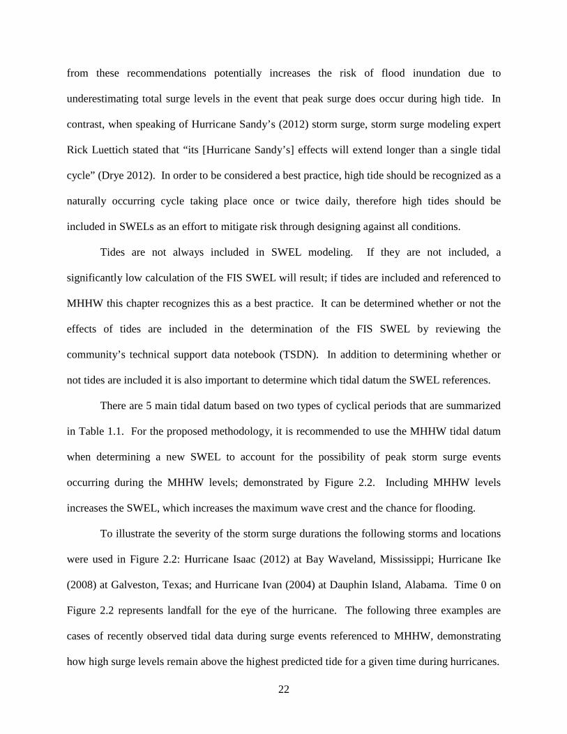
from these recommendations potentially increases the risk of flood inundation due to

underestimating total surge levels in the event that peak surge does occur during high tide. In

contrast, when speaking of Hurricane Sandy’s (2012) storm surge, storm surge modeling expert

Rick Luettich stated that “its [Hurricane Sandy’s] effects will extend longer than a single tidal

cycle” (Drye 2012). In order to be considered a best practice, high tide should be recognized as a

naturally occurring cycle taking place once or twice daily, therefore high tides should be

included in SWELs as an effort to mitigate risk through designing against all conditions.

Tides are not always included in SWEL modeling. If they are not included, a

significantly low calculation of the FIS SWEL will result; if tides are included and referenced to

MHHW this chapter recognizes this as a best practice. It can be determined whether or not the

effects of tides are included in the determination of the FIS SWEL by reviewing the

community’s technical support data notebook (TSDN). In addition to determining whether or

not tides are included it is also important to determine which tidal datum the SWEL references.

There are 5 main tidal datum based on two types of cyclical periods that are summarized

in Table 1.1. For the proposed methodology, it is recommended to use the MHHW tidal datum

when determining a new SWEL to account for the possibility of peak storm surge events

occurring during the MHHW levels; demonstrated by Figure 2.2. Including MHHW levels

increases the SWEL, which increases the maximum wave crest and the chance for flooding.

To illustrate the severity of the storm surge durations the following storms and locations

were used in Figure 2.2: Hurricane Isaac (2012) at Bay Waveland, Mississippi; Hurricane Ike

(2008) at Galveston, Texas; and Hurricane Ivan (2004) at Dauphin Island, Alabama. Time 0 on

Figure 2.2 represents landfall for the eye of the hurricane. The following three examples are

cases of recently observed tidal data during surge events referenced to MHHW, demonstrating

how high surge levels remain above the highest predicted tide for a given time during hurricanes.

22

Figure 2.2 Tidal Gauge Data Collected by NOAA Co-Ops Buoys During Hurricanes (A) 2004 Ivan, (B) 2008 Ike, and (C) 2012 Isaac

In all three cases, the peak surge occurred almost simultaneous with the normal predicted high

tide. The maximum surge elevation above the predicted high tide level was 6.19 feet for

Hurricane Isaac, 10.2 feet for Hurricane Ike, and 7.99 feet for Hurricane Isaac. The maximum

surge levels above the normal GT (MHHW to MLLW range) associated with the selected storms

are 459% above the 1.74 foot GT for Waveland, MS. (Currents, 2012a); 500% above the 2.04

foot GT for Galveston, TX. (NOAA Tides & Currents 2012); and 515% above the 1.20 foot GT

for Dauphin Island, AL. (NOAA Tides & Currents 2012).

Figure 2.3 shows the duration of the surge elevations from Figure 2.2 as the percentage of

a 24-hour day for three intervals of the maximum surge level: 40%, 60%, and 80%. A value on

23

the Y axis above 100% indicates that the indicated level of surge was experienced at the station

location for greater than one 24-hour day.

Figure 2.3 Percentages of the Maximum Surge Elevation Shown as a Percentage of a 24-hour Day.

For the selected hurricanes, 40% of the maximum surge elevation occurs simultaneously

with the predicted high tide for 79% to 197% of a 24-hour day; 60% of the maximum surge

elevation occurs simultaneously with the predicted high tide for 34% to 147% of a 24-hour day;

and 80% of the maximum surge elevation occurs simultaneously with the predicted high tide for

16% to 98% of a 24-hour day. These statistics verify the need to include high tide effects with

an estimated storm surge level by demonstrating through past events the high likelihood of

elevated surge levels occurring simultaneously with the predicted high tide. Additionally, two of

the three examples (‘A’ Ivan and ‘C’ Isaac) are only indicative of a diurnal tidal cycle, one high

and low per day, representing a lower likelihood of simultaneous occurrence than a mixed or

semi-diurnal cycle (‘B’ Ike). Thus, if the tidal cycle is mixed or semi-diurnal, two high and low

tides per day, the possibility of simultaneous high tides and peak surge levels is doubled on the

average.

79% 99%

197%

34% 68%

147%

16% 23%

98%

0%

50%

100%

150%

200%

250%

Ivan Ike Isaac

% o

f 24-

Hou

r Day

% of Maximum Surge Elevation for % of 24-Hour Day

40% of Maximum Surge Elevation60% of Maximum Surge Elevation80% of Maximum Surge Elevation

24

As demonstrated above in Figure 2.2 and 2.3, storm tides can be abnormally high for a

duration extending across multiple high tides thus increasing the opportunity for the two to occur

simultaneously. Therefore, incorporating MHHW rather than a weighted average of high and

low tides accounts for the highest risk associated with natural tidal cycles given at least one high

and low tide per day tides and simultaneous peak storm surge elevations. To prevent damage by

elevating above flood waters, making sure MHHW is included in the DFE is imperative.

2.3.4 Flood Return Intervals

Within the expected 60 year lifespan of a typical building, defined as an ASCE risk

category II structure (ASCE 2010), the probabilities of the 100-, 500- and 700-year events

occurring during a 60-year useful life are 45%, 11%, and 8% respectively (Friedland and Gall

2012). This level of risk associated with flood return periods is inconsistent with wind design

risk levels. ASCE 7 requires the following design levels for wind events (ASCE 2010):

• Risk category I structures, defined as those that represent a low risk to human life in the

event of failure, to be designed for wind speeds that correspond to the 300-year mean

recurrence interval (MRI)

• Risk category II structures, defined as all buildings and structures except those listed as I, III,

and IV, shall be designed for wind speeds that correspond to the 700-year MRI

• Risk category III and IV structures, defined as buildings and structures which pose a

substantial hazard to the community and substantial risk to human life, shall be designed for

wind speeds that correspond to the 1700-year MRI

While the minimum design standard for wind is the 300-year MRI, the maximum design

standard for flood is the 100-yr MRI. As hurricanes are a hazard with coupled risk (i.e. wind and

coastal flooding), this incredible imbalance of risk is not in line with current optimized risk-

based design.

25

FEMA provides minimal guidance for designing above the 100-year BFE. A minority of

FIS have started to provide a 500-year SWEL, but if this is not available then the only guidance

for design beyond 100-yr elevations is provided by FEMA as rule of thumb to approximate the

500-year Stillwater elevation (SWEL) as 1.25 times the 100-year Stillwater elevation (FEMA

2002; FEMA and NAHB Research Center 2010). In addition, the CCM mentions that an AHJ

may specify a non-100-year frequency-based DFE to be used (FEMA 2011). There is no real

guidance for developers to use when trying to design for flood events with longer return periods.

2.4 Proposed Design Practices

The proposed methodology to determine a DFE for the LHSM combines ASCE, CCM,

and recommended practices for bridging the gaps in current code and practices. The

methodology may be used in conjunction with any selected storm recurrence interval and is not

restricted to the 100-year storm. The proposed practice presents new information in addition to

referencing guidance from other sources such as the CCM.

The equations proposed to calculate the recommended DFE reflected in column five are

presented in Equations 2.1 through 2.12. Each of the variables is discussed in further detail in

the following subsections, including appropriate usage and origin or derivation of the associated

equations.

SWEL88 = SWELFIS +/- Conversion (2.1) SWELPRIOR = (Datecons – Datemodel)* HistoricGSLR + SWEL88 (2.2) SWELGSLR = SWELPRIOR + (GSLR x LIFE) (2.3) SWELMHHW = GT/2 + SWELGSLR (2.4) SWELMHHW = (MN/2 - GT/2) + SWELGSLR (2.5) GroundSUB = GroundExist - (RateSUB*LIFE) (2.6) Elandward = ELong-term x LIFE (2.7)

26

where:

SWELFIS is the elevation taken from FIS

Conversion = the output offset between NGVD 29 and NAVD 88 from the vertical

transformation program. Note: an actual elevation may be given and used as ‘SWEL88’

rather than an offset equation.

SWEL88 = the adjusted elevation from the datum conversion now referenced to NAVD 88

SWELPRIOR = SWEL resulting from GSLR amount occurring between effective SWEL model date

and construction start date

Datecons = the date construction is to begin on the structure

Datemodel = the modeling date of the current SWEL as published in the FIS

HistoricGSLR = the published historical rate of GSLR; or amount of rise as a number over the

given time period. If Datemodel is after 1990, HistoricGSLR rate = GSLR

SWELGSLR = the total combined effects of GSLR that occur prior to construction of the structure

and over the structure’s useful life

GSLR = the projected global sea level rise rate over the specified time frame

LIFE = the useful life of the structure in years

SWELMHHW = the SWEL referenced to Mean Higher High Water tidal datum

GT = the great diurnal tide range (MHHW-MLLW)

MN = Mean Range of Tide (MHW-MLW)

Drop = DProfile x Elandward (2.8) GS = GroundSUB – Drop (2.9) dproposed = SWELMHHW – GS (2.10) Proposed dfp = ((dproposed * 0.78)*0.7) + dproposed (2.11) DFEPROPOSED = Proposed dfp + GS (2.12)

27

GroundSUB = New ground elevation after accounting for effects of subsidence

GroundExist = existing ground elevation

RateSUB =Rate of subsidence

Elandward = the amount of feet the shoreline translates horizontally towards the building

ELong-term = the long-term landward erosion rate of the shoreline; CCM recommends using a

minimum rate of 1.0 ft/yr (FEMA 2011);

Drop = the amount in feet that the ground elevation drops at the seaward row of piles

DProfile = the calculated eroded dune profile; CCM uses a vertical to horizontal ratio of 1:50

(FEMA 2011)

GS = eroded ground elevation; need to reference NAVD 88 for the proposed methodology.

dproposed = the design stillwater depth

0.78 = the coefficient for the maximum breaking wave height of a depth-limited wave

0.70 = the coefficient of the percent of the breaking wave height that lies above the SWEL

Proposed dfp = the Proposed design flood protection depth

DFEPROPOSED = the Design Flood Elevation resulting from the proposed methodology

2.4.1 Datum Conversion

The FIS and FIRM can be used to determine which vertical datum is used. If the FIRM

and FIS reference NAVD 88, this section may be skipped and SWEL calculations can be

resumed with Section 2.4.2. FEMA FIS can be used to determine the desired return period flood

SWEL from the generally included 10-, 50-, and 100-year storms, with newer FIS including 500-

year storms. Other recurrence intervals may be used provided they are approved by an AHJ.

FIS include transect locations and data providing the approximate location of the elevations. The

transect closest to the site of the structure with the SWEL corresponding to the desired storm

frequency in the FIS summary of transects table will yield the most accurate results.

28

Programs such as Corpscon, VERTCOM or VDatum may be used for vertical datum

transformations from NGVD 29 to NAVD 88. Of the coastal FIS evaluated for this thesis, most

are still referenced to NGVD 29. The latitude, longitude, SWEL, and horizontal projection used

for the structure’s geographic location are typically necessary for such vertical datum

transformations. To perform the vertical datum transformation, the SWEL elevation is the input

variable, NGVD 29 is the input datum, and NAVD 88 is the output vertical datum. The

transformation results in a new elevation referenced to NAVD 88, hereafter indicated as

SWEL88. If the vertical transformation program used produces an output showing a vertical

offset rather than an elevation, Equation 2.1 can be used to arrive at the new SWEL88.

2.4.2 Effects of GSLR

To account for the total GSLR, it may first be necessary to include GSLR between the

effective SWEL model date and construction start date. When using the effective date of the

FIS, it is necessary to review prior versions of the FIS and determine the modeling date for the

current SWEL (Datemodel). A difference in the modeling date and the effective date of the FIS is

not uncommon. Therefore, using the modeling date accounts for the total amount of sea level

rise determined from the date of modeling until the date of construction and should be added to

the SWEL. If the modeling date is prior to 1990, then documented historical rates of GSLR

should be used to better represent actual conditions. After 1990, HistoricGSLR (Equation 2.2) is

estimated based on the recommendation of using a linearly projected rate of 0.03 ft/yr. To

determine the new SWEL resulting from GSLR that has occurred from the modeling date of the

FIS SWEL until construction begins, Equation 2.2 should be used. The result, SWELPRIOR,

should be added to the GSLR that is expected to occur over the useful life of the structure

(Equation 2.3).

29

To determine GSLR over the useful life of the structure, the process proposed in the

CCM is recommended (FEMA 2011, 8-13). As recommended in the CCM (pg 8-13), the 100-

year SWEL should be increased by the product of the GSLR rate (0.03 feet per year) and the

expected useful life of the structure (FEMA 2011). The result should be combined with

SWELPRIOR (Equation 2.3) to obtain SWELGSLR, which includes all effects of GSLR after the

modeling date of the SWEL.

2.4.3 Tidal Influence

If possible, determine if the SWEL modeling is calibrated to MHHW, if it does not

reference MHHW, determine which tidal datum the SWEL references. On occasion a tidal

datum may be noted in the Flood Insurance Study, but of the observed FIS, most mention only

astronomical tide calibration in the modeling process, which includes a weighted average of high

and low tides (FEMA 2007). If not found in an FIS, the technical support data notebook (TSDN)

can be reviewed to determine how the astronomic tide is calibrated for the modeling process. In

order to design for the highest possible flood elevation associated with a surge event, it is

proposed that the SWEL accounts for the highest predicted tide for a single day; known as Mean

Higher High Water (MHHW). To account for high tides it is necessary to use the great diurnal

tide range, GT, or the mean range of tide, MN, of the nearest tidal station from

tidesandcurrents.noaa.gov. Step 2.4.3, Account for Tides, will use only one of the following

options below: for a MSL SWEL step 2.4.3.1 is recommended, for a MHW SWEL step 2.4.3.2 is

recommended, and for a MHHW SWEL it is recommended to proceed to step 2.4.4.

2.4.3.1 Mean Sea Level (MSL)

If a SWEL is only referenced to MSL (no tides) it is recommended to add the difference

between MHHW and MSL to the SWEL to provide a more effective SWEL. To adjust from

30

MSL to MHHW, Equation 2.4 can be used. The GT is the difference between MHHW and

MLLW for both semidiurnal (mixed) cycles and diurnal cycles.

2.4.3.2 Mean High Water (MHW)

In the context of a semidiurnal (mixed) tide cycle, MHW is the average of the lower of two daily high tides observed over a tidal epoch. A diurnal cycle is not referenced to MHW, its high tide is known as MHHW. If a SWEL is referenced to MHW, it is recommended to be changed to reference MHHW to be considered a best practice. In order to adjust a SWEL from MHW to MHHW, Equation 2.5 can be used to arrive at the desired elevation.

At the conclusion of step 2.4.3, the result SWELMHHW, comes from either step 2.4.3.1 or

2.4.3.2 and should be carried through the remainder of the methodology. At the end of this step

SWELMHHW is still an elevation. The goal of step 2.4.3 is to have all SWEL’s referenced to

MHHW in order to achieve the best-recommended practice.

2.4.4 Determine Lowest Eroded Ground Elevation (GS) and Erosion Effects

In the CCM there is a methodology to determine the lowest eroded ground elevation at

the seaward row of columns/ piles. The lowest eroded ground elevation is necessary if

attempting to determine the maximum wave crest of depth-limited breaking waves. GS

determination is a four-step process as explained by methods in the CCM.

2.4.4.1 Lower Existing Ground Elevation by Amount of Subsidence Over Life of Structure

To lower the existing ground elevation by the amount of subsidence, it is recommended to

subtract the product of the documented rate of subsidence and the useful life of the structure

from the existing ground elevation; CCM pg 8-8 (FEMA 2011). See Equation 2.6.

2.4.4.2 Landward Movement of Sand Dune

Determine how far the seaward toe of the dune translates horizontally toward the building: CCM

pg 8-14 (FEMA 2011). Equation 2.7 may be used to find ELANDWARD.

31

2.4.4.3 Eroded Ground Elevation at Seaward Row of Piles

Finding the amount the ground will drop at the seaward row of piles considering the slope of the

eroded dune is recommended because it affects the overall SWEL and wave effects; view CCM

pg. 8-14 (FEMA 2011). Dune erosion characteristics are covered in chapter 3 and 8 of the CCM.

Equation 2.8 can be used to find ‘Drop’.

2.4.4.4 Determine GS

The eroded ground elevation can be found using the existing ground elevation and the calculated

drop from step 2.4.4.3 above; see CCM pg 8-14. Equation 2.9 can be used to find GS.

2.4.5 Find the Design Stillwater Depth, ds.

The design stillwater depth is the difference in SWELMHHW, found in step 2.4.3, and the

GS, found in step 2.4.4.4. This difference as presented in the CCM is defined as the final design

stillwater depth, dS, before wave calculations are included. The proposed methodology refers to

this difference as dproposed given there are differences in the proposed methodology and the CCM.

It is important to note that this step is necessary to define the flood depth rather than the

elevation in order to determine the maximum depth-limited wave crest in step 2.4.6. At the

beginning of this step, 2.4.5, SWELMHHW and GS are both elevations, but the difference between

the two, dproposed, in Equation 2.10 is a depth to be used in step 2.4.6.

2.4.6 Maximum Wave Crest

Using dproposed from step 2.4.5, the maximum wave crest can be found using techniques in

the CCM (proposed Equation 2.11). The result is the design flood protection depth from the

proposed method, indicated by the variable ‘proposed dfp’ or ‘dfp’ for the CCM (FEMA 2011).

2.4.7 Design Flood Elevation

The result of step 2.4.6, proposed dfp, is a flood depth, which is recommended to be

converted back into an elevation in order to get an approved certificate of elevation. Using the

32

lowest eroded ground elevation, GS, from the method provided in the CCM (step 2.4.4.4), add to

Proposed dfp from step 2.4.6, to get an elevation referenced to NAVD 88 (Equation 2.12). It is

recommended that all BFEs and DFEs are rounded to the nearest whole foot as are done on

FIRMS. At the completion of step 2.4.7 the result is the proposed DFE: DFEPROPOSED.

2.5 Summary of Code, Code-Plus and Recommended Practices

Table 2.2 summarizes ASCE, IBC & IRC code requirements, CCM best practices,

recommended practices to close gaps within the CCM recommendations, and the input required

for each computation. The final row of the table provides a DFE for code requirements and the

recommended practices, and provides a design flood protection depth (dfp) for the CCM

practices. Slight alteration to the dfp by adding to the lowest expected ground elevation will yield

a DFE for the CCM. Code requirements are summarized in column three in addition to the

freeboard amounts associated with each ASCE category and the respective LHSM orientation to

the direction of wave approach. Column four describes the practices provided by the CCM.

Column five combines CCM recommendations with proposed practices to address the gaps

discovered within the CCM. The end result of column five is the proposed DFE.

2.6 Case Study

A case study for St. Johns County, Florida, is used to demonstrate the differences among

SWEL elevations from the three methods summarized in Table 2.2. The case study provides all

of the necessary information and characteristics a practitioner would need to follow the proposed

methodology presented in Section 2.4. In addition, calculations are shown in the case study.

The differences in the elevation requirements for code, CCM practices, and the proposed method

are show in Figure 2.4 and discussed in detail. DFEs for the case study are rounded to the

nearest foot as done in practice and for BFE values specified on FIRMs.

33

Table 2.2 Code, Best Practices, and Recommended Practices Summary

Variables Input Data IBC*, IRC*, and ASCE 1 Coastal Construction Manual (CCM) Recommended Best Practices Vertical Datum • Vertical datum for SWEL

• Difference in vertical datum Specified on community’s FIRM Specified on community’s FIRM

1. Before continuing, make sure all elevations reference NAVD 88.

Global (Eustatic) Sea Level Rise (GSLR)

• Published GSLR rate • Building lifetime • SWEL • Model date of effective SWEL • Date of construction

--

Add the product of the GSLR rate and the building lifetime to the effective SWEL. [CCM Fig 8-3]. This results in ESW.

2. Include GSLR from modeling date of effective SWEL through date of Construction. This will increase the SWEL 3. Include CCM direction.

Tides • Are tides included in the FIS modeling?

• If so, to which tidal datum is it referenced?

-- --

4. Include the highest tide (MHHW) with DFE. This increases the SWEL (ds for CCM). Resulting in dPROPOSED: best practice SWEL depth.

Subsidence • Published rate of subsidence • Building lifetime • Existing ground elevation

-- Lower the existing ground elevation by the product of the subsidence rate times the building lifetime. [CCM Fig 8-3]

5. Follow CCM recommendations

Erosion (landward)4 • Long-term erosion rate • Building lifetime • Historical landward shoreline

-- Measure landward from historical shoreline by the product of the erosion rate and the building lifetime. [CCM Fig 8-3]


Lowest expected ground (due to erosion)

• Expected landward shoreline • Eroded dune profile from

storm erosion model or stable bluff profile using available guidance and data

--

Using the most landward expected shoreline, calculate an eroded dune profile. Lower the ground elevation calculated from subsidence by eroded dune amount at the seaward row of piles, The result from steps 2-4 is GS.


Maximum Wave Crest Calculation

• For IRC, IBC, ASCE: • FIS • For CCM: • ds • 0.78ds= max breaking wave ht • 0.7(max breaking wave ht)

Included in BFE calculation

Calculate: ds = ESW – GS (EQ 8.1 CCM). ESW is calculated in step 2, and GS is derived in steps 2-4. Multiply ds by 0.78, resulting in the breaking wave height; then multiply this height by 0.7 and add back to the ds giving you the dfp

8. Multiply Best Practices stillwater depth, dPROPOSED, by 0.78,= breaking wave height (Hb); then multiply by 0.70 and add to dPROPOSED = Proposed dfp: ((dPROPOSED * 0.78)*0.7) + dPROPOSED = Proposed dfp

Bottom of LHSM Elevation Requirements (IRC, IBC, ASCE, CCM) OR, LHSM depth (CCM): High Hazard Areas- V-Zones

• For IRC, IBC, ASCE: • BFE • Orientation of LHSM • Community adopted freeboard • dfp

Category I structure: DFE 2, 3 Category II Structure: higher of DFE 2 or of BFE+ 1’ 2, 3 Category III & IV Structures: Higher of BFE + 1’ or DFE2; or Higher of BFE + 2’ or DFE3

Use the design flood protection depth, dfp, calculated above in step 5. OR Add dp back to GS for elevation referenced to original datum of FIS (DFE).- not an official CCM recommendation

9. Using Proposed dfp, add GS from step 6 (calculated in step 4 of CCM method) to arrive at LHSM elevation referenced to NAVD 88. Proposed dfp + GS = DFEPROPOSED

* IBC 1612.4 & IRC R322.1 Floodway construction must be in accordance with ASCE 24 (ICC 2009; ICC 2011). 1- Use in conjunction with Table 4-1 of ASCE 24. 2- LHSM is parallel to wave approach, where LHSM is ≤ 20 degrees from the direction of approach (ASCE 2005; ICC 2009). 3- LHSM is perpendicular to wave approach, where LHSM > 20 degrees from direction of approach (ASCE 2005; ICC 2009). 4- It is recommended that a minimum rate of 1.0 ft/year is used unless durable shoreprotection or erosion-resistant soil is present (FEMA 2011)

34

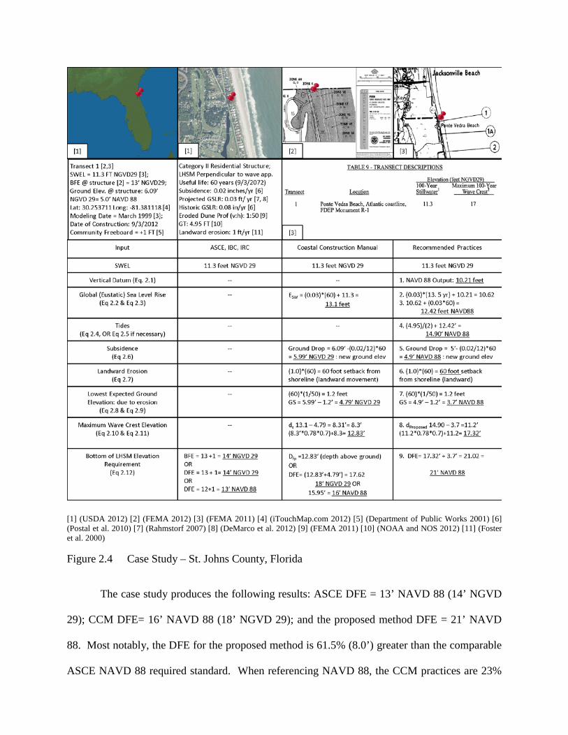
[1] (USDA 2012) [2] (FEMA 2012) [3] (FEMA 2011) [4] (iTouchMap.com 2012) [5] (Department of Public Works 2001) [6] (Postal et al. 2010) [7] (Rahmstorf 2007) [8] (DeMarco et al. 2012) [9] (FEMA 2011) [10] (NOAA and NOS 2012) [11] (Foster et al. 2000) Figure 2.4 Case Study – St. Johns County, Florida

The case study produces the following results: ASCE DFE = 13’ NAVD 88 (14’ NGVD

29); CCM DFE= 16’ NAVD 88 (18’ NGVD 29); and the proposed method DFE = 21’ NAVD

88. Most notably, the DFE for the proposed method is 61.5% (8.0’) greater than the comparable

ASCE NAVD 88 required standard. When referencing NAVD 88, the CCM practices are 23%

35

(3.0’) higher than the required ASCE standard and the proposed methods remain 31% (5’) higher

than the best available current practices.

FEMA’s recommendation to multiply the 100-year SWEL by 1.25 to arrive at an

approximate 500-year SWEL yields a 20’ NAVD 88 DFE (22’ NGVD 29) at the location of the

case study (FEMA 2002). The approximated NAVD 88 500-yr DFE from FEMA is 5% (1’) less

than the 100-year DFE resulting from the proposed method. In addition, the St. Johns County

FIS (from the case study) provides a 500-year SWEL, but no 500-year wave crest (FEMA 2011).

Using the same methods in the FIS and case study to determine the 100-year wave crest, the

approximate 500-year wave crest based on the given 500-year SWEL, 12.2’ NGVD 29 (FEMA

2011), is equal to 18.86’ NGVD 29 = 17.17’ NAVD 88; a 19’ and 17’ DFE, respectively. The

proposed method 21’ DFE that considers future conditions is still 23.5% (4’) higher than the

approximated 500-year 17’ NAVD 88 DFE using data from the FIS.

Although the proposed method DFE provided in the case study is already higher than the

other options, it is important to note in the first step, datum conversion, that there is actually a

negative conversion. The shift from NGVD 29 to NAVD 88 actually reduced the SWEL by 1.09

feet, though this is not always the case. In Grand Isle, Louisiana there is a positive change of

0.14 feet between the vertical datum (USACE 2009). Therefore, if this same study were

performed for Grand Isle, LA the SWEL would increase by +1.23 feet (1.09 + 0.14) for the

datum conversion alone when compared with the given case study.

Given the statistical differences among the DFEs, it is important to note that including the

future effects of geological processes can reduce the likelihood of flooding. Not including future

effects of coastal geological processes can significantly increase the risk of flooding. For

example, including just the effects of subsidence and GSLR over the expected useful life for the

structure (60 years) at the site of the case study effectively reduces the FIRM DFE (14’ NGVD)

36

by 13.6% or 1.9 feet. The overall difference in accounting for all future effects, as the proposed

method does, and not accounting for any future effects, like the current design standard, is a

difference of 61.5% (8’) in the DFE at the end of the structure’s useful life.

2.7 Conclusion

The underlying premise of flood protection in coastal zones is to eliminate flood waters

from infiltrating the structure altogether. Design Flood Elevations are the absolute minimum

elevation for new construction, and are determined according to NFIP and ASCE standards.

Current codes and standards (e.g. ASCE, IBC, and IRC) do not include methodologies for

designing above the 100-year DFE, nor do they consider the effects of characteristics of the

changing coastal environment. In contrast, the CCM includes the effects of future coastal

processes, although it does not address all of the necessary aspects, including vertical datum

conversions, global sea level rise that occurs prior to construction of the building and the effects

of high tides during peak surge intervals.

This chapter presents a comprehensive methodology to determine the DFE if the design

SWEL is known that addresses these remaining challenges and combine the current best

available practices to provide a comprehensive guide for practitioners wishing to evaluate each

source of flood risk. The methodology was developed based on an evaluation of coastal

phenomena such as tides, sea level rise and subsidence. These phenomena are recognized as

physical processes, and it is the authors’ contention that they should be explicitly accounted for

in the determination of flood elevation. The case study that implemented this methodology for

St. Johns County, Florida, resulted in a DFE that was 61.5% (8’) higher than a DFE calculated

following current code requirements and 31% (5’) higher than would be calculated using the

CCM.

37

Code revision should better educate practitioners for flood considerations. Designers are

aware of code requirements but they might not even be aware of best available practices such as

the CCM. In addition, best practices should be incorporated into code requirements with

modifications to those that neglect certain aspects. To account for subsidence, code revision

should provide subsidence rate maps, including developing maps for areas that don’t yet have

one. To incorporate MHHW, code revision should provide information about including tides

given that tidal data is readily available but not addressed. Tides should be accounted for in

design, and more explicit information about the consideration of tides should be included in FIS.

Code and best practices neither explicitly state nor provide any guidance to the designer for

converting between vertical datums. Code should provide guidance in converting between

vertical datum including recommending such conversion programs in addition to highlighting the

importance of referencing the correct elevation to the correct vertical datum.

There is not adequate information available for practitioners about flood practices and

requirements. Practitioners are restricted to elevating to the 100-year BFE with occasional 500-

year SWEL guidance. Only the 100-year BFE is a code requirement, but even if provided with a

500-year SWEL there is no intermediate guidance. In addition, it should be recognized that the

100-year BFE is only a minimum design requirement, and not a best practice. It seems that most

homeowners want to only build to the minimum required elevation (the BFE), yet they should be

better informed by developers of the risk associated with designing only to the absolute

minimum requirements.

This chapter is not suggesting the presented methods become requirements, but it does

focus on estimating the actual 100-year BFE which considers future effects of the coastal

processes during the lifetime of the structure. It should also be noted that comprehensive

methods can both over-account and under-account for future effects. Policy and insurance

38

related issues should be separated from the requirements of engineering design. Engineering

design should be focused on protecting human-life and structures, not to determine insurance

rates. Insurance rates may still be tied to elevation, but it should reference the best available

practice; elevate below the best practice and pay a higher rate, elevate at or above the best

practice elevation and pay a lower premium.

2.8 Acknowledgements

The authors would like to acknowledge financial support from LSU’s Coastal

Sustainability Studio and technical information from Russell “Joey” Coco, Jr., Dr. Lynne Carter

and Adam Reeder.

39

CHAPTER 3: ESTIMATING COASTAL FLOOD ELEVATIONS FOR RETURN PERIODS EXCEEDING CURRENT NFIP GUIDANCE USING EXISTING FIS

3.1 Introduction

Determination of the design flood elevation (DFE) for buildings constructed in the

floodplain is currently tied to policy requirements of the National Insurance Flood Program

(NFIP) 100-year flood. Additional protection is provided by freeboard, which is intended to

compensate for factors that can result in greater flood depths (FEMA 2011). Freeboard,

however, is an arbitrary value that is expected to compensate for multiple known and unknown

factors. In applying freeboard, protection beyond the 100-year event is provided, but there is no

indication of the failure probability that results from the application of freeboard. Additionally,

for the practitioner wishing to estimate DFEs for failure probabilities beyond the 100-year event,

information is very limited. Thus, those wanting to plan for a higher level of risk may struggle to

find methods that can even estimate the DFE for these events. There is therefore a need to

develop a methodology to estimate longer return period flood elevations using information

readily available to practitioners.

Current codes, standards, and even best practices are based on the 100-year flood for all

classifications of structures. This indicates a lack of understanding of the risk associated with

designing to the 100-year flood. Within the expected 60-year lifespan of a typical residential

structure, defined as a risk category II in ASCE 24 (ASCE 2010), the probabilities of the 100-,

500- and 700-year events occurring at least once are 45%, 11%, and 8% respectively (Friedland

and Gall 2012). Furthermore, the 100-year flood has a 26% (1in 4) change of occurring over the

life of a 30-year mortgage (FEMA and Federal Insurance and Mitigation Administration 2002).

This level of risk (1% annual probability of failure) is much higher than the acceptable risks of

failure for other hazards. According to the ASCE 7 commentary Table C.1.3.1a, the highest

40

acceptable annual probability of failure for load conditions (excluding earthquake hazards) is

0.0125% (ASCE 2010). This discrepancy in acceptable risk is especially critical in coastal flood

areas, where waves and hydrodynamic forces can easily destroy buildings when the design flood

elevation is exceeded. The acceptable level of risk for flooding should be lower by providing

guidance on how to determine flood elevations of longer return periods.

FEMA provides flood insurance studies (FIS), which detail the methods and data used to

map the 100-year base flood elevation (BFE) on flood insurance rate maps (FIRMs). At a

minimum, the FIS provides a 100-year stillwater elevation (SWEL) which serves as the basis for

delineating BFE values on a FIRM. The FIS may also provide the 10- and 50-year SWELs, with

newer FIS providing a 500-year SWEL. Although more communities are providing 500-year

SWELs, the corresponding annual probability of exceedance for the 500-year event is 0.2%, still

significantly higher than the target acceptable limits. Therefore, additional guidance is needed

for practitioners wishing to estimate flood elevations for the more commonly accepted risk of

failure values. This chapter will analyze FIS SWEL values to estimate SWELs for longer return

periods.

Various statistical distributions have been used to fit extreme values in hydrology. These

methods include but are not limited to log normal, Gumbel, Beta-P, log-log or Huff-Angel, and

semi-log or SRCC (Angel et al. 1992; Needham 2010). Huff-Angel is a log-log regression

technique that is used to estimate rainfall frequencies and extremes for the Midwestern United

States (Angel et al. 1992), and the Southern Regional Climate Center (SRCC) regression method

is log-liner and has been implemented to estimate rainfall frequencies and extremes for the

south-central states (Faiers et al. 1997). The ‘fitness’ of a method to a dataset can be determined

using the Kolmogorov-Smirnov (KS) statistic, with a lower KS value representing a better fit

(Keim and Faiers 2000; Needham 2010). The values for extreme events produced by Huff-

41

Angel and SRCC have been shown to fall within the lower extreme of Gumbel (Wilks and

Cember 1993; Needham 2010) and the upper extreme of Beta-P (Needham 2010). Therefore,

Huff-Angel and SRCC will be used to fit regression equations to SWEL data obtained from FIS

for select communities along the Atlantic and Gulf Coasts.

3.1.1 Background on NFIP and the 100-year flood

In 1965, Congress directed the Department of Housing and Urban Development (HUD)

to conduct a comprehensive study of flood insurance following significant losses from Hurricane

Betsy (Power and Shows 1979). Marion Clawson, then secretary of HUD, completed the study

in 1966 that recommended a federally sponsored flood insurance program (Power and Shows

1979). The National Flood Insurance Act of 1968 (NFIA) followed, which established the NFIP

with the purpose of (Power and Shows 1979):

• Better indemnifying individuals for flood losses through insurance (FEMA and Federal

Insurance and Mitigation Administration 2002);

• Reducing future damages through state and community floodplain management regulations

(FEMA and Federal Insurance and Mitigation Administration 2002); and

• Reducing federal expenditures for disaster assistance flood control (FEMA and Federal

Insurance and Mitigation Administration 2002).

The National Flood Insurance Act of 1968 explicitly intended for the NFIP to be “a

program of flood insurance with large-scale participation of the Federal Government and carried

out to the maximum extent practicable by the private industry” (Office of the General Counsel

1997, 1).

When the National Flood Insurance Program (NFIP) was mandated to map all the

floodplains in the U.S., it became necessary to determine a standard “size” event in order to

assess and manage flood risk for determination of insurance rates, thus treating all communities

42

equally (FEMA and Federal Insurance and Mitigation Administration 2002). Approximately 50

researchers in the field of floodplain management were identified and invited to participate in a

floodplain management guidelines seminar at the University of Chicago that was held December

16-18, 1968 (Sheaffer 2004). The 100-year BFE was established at the recommendation of these

50 research experts who were convened by the U.S. Department of Housing and Urban

Development (HUD) to determine a standard to be used as the “basis for risk assessment,

insurance rating, and floodplain management for the NFIP" (FEMA and Federal Insurance and

Mitigation Administration 2002, 5). The 100-year flood was a compromise between a 50-year or

lesser standard and a 500-year flood standard (Krimm 2004). Thus the 100-year flood standard,

or the flood with a 1%-annual-chance of occurrence, was adopted by the Federal Insurance

Administration (FIA) and was used to identify floodplains (Krimm 2004).

In the 1960’s, both the USACE and the Tennessee Valley Authority (TVA) agreed upon

the 100-year flood as a uniform standard for flood protection (Robinson 2004). On September

10, 1971, the NFIP specifically tied the regulatory requirements of the program to the 100-year

flood standard (Robinson 2004). In May 1972, the U.S. Water Resources Council issued final

guidelines for evaluating flood hazards that recommended agencies use the 100-year flood as the

“basic flood” (Robinson 2004, 3). The 1973 enactment of PL 93-234 (1972 Act, as amended)

affirmed the use of the 1% or greater chance of flooding (100-year flood) as the “base flood

standard” (Reilly 2004, 14). In 1974 amendments to the NFIA, the 100-year flood was

specifically mentioned in the NFIP legislation for the first time (Robinson 2004), and on October

26, 1976, the term “base flood” and “base flood elevation” were introduced to phase out the

misleading term of the “100-year flood” (Robinson 2004, 5).

On May 24, 1977 President Jimmy Carter issued Executive Order (EO) 11988-

Floodplain Management, which specifically defines the floodplain as the base flood in terms of

43

the 100-year flood (Reilly 2004; Robinson 2004). The sufficiency of the 100-year flood was

reviewed in 1973 by the Senate Committee on Banking, Housing, and Urban Affairs, and again

in 1981 by the Office of Management and Budget (OMB) as part of the President’s 1981 Task

Force on Regulatory Relief. In both of these reviews, the 1-percent-annnual-chance standard

was deemed “reasonable and consistent with national objectives in reducing flood losses”

(FEMA and Federal Insurance and Mitigation Administration 2002, 5). A 1983 report by the

Presidential Task Force on Regulatory Relief concluded that no better alternatives to the

standard were available and that there was no justification for the expense of converting to

another standard (Foundation 2004).

Congress passed the Flood Disaster Protection Act of 1973, which provided strong

incentives for community and individual participation in the flood insurance program by

introducing broad financial penalties for failure to participate (Power and Shows 1979). Section

102(a) and 102(b) of this act were intended to prevent lending by savings and loan institutions if

an identified flood-prone community did not participate in the flood insurance program (Power

and Shows 1979). “Section 1315 of the 1968 Act prohibits FEMA from providing flood

insurance unless the community adopts and enforces floodplain management regulations that

meet or exceed the floodplain management criteria established in accordance with section

1361(c) of the Act” (FEMA and Federal Insurance and Mitigation Administration 2002, 12).

Changes made to the program in 1969 and 1973 dramatically increased participation, increasing

the number of participating communities from four in 1969 to 15,898 in 1978, leaving only 2,928

(as of 1978) officially identified flood-prone communities that had yet to join (Power and Shows

1979).

44

3.1.2 Probability of Exceedance

The probability of an annual maxima-specific event occurring during the lifetime of a

building is known as the probability of exceedance. Table 3.1 below demonstrates the

probability of exceedance for mean recurrence interval (MRI) events compared to the expected

useful life of a building. A recurrence interval is the reciprocal of probability (Markowitz 1971).

Table 3.1 Probability of Exceedance for Events During Expected Useful Life (Friedland and Gall 2012)

The probability of exceedance may be calculated using Equations 3.1 and 3.2:

Pnot = (1 - 1𝑋𝑋

)n (3.1)

Poccur = 1 - Pnot (3.2)

where:

Pnot = the probability of an event not occurring in ‘n’ years,

xx = the return period of the event in years,

n = number of years the event does not occur, and

Poccur = the probability of the event occurring at least one time in ‘n’ years.

3.1.3 Return Periods and Annual Maxima

When using the term ‘500-year flood’ or ‘100-year flood’, it is easy to perceive this event

occurring only once every 500 years or once every 100 years, when in actuality, the flood has a 45

0.2% chance or 1.0% chance of occurring annually, respectively (Philippi 1994). Therefore, an

October 26, 1976 Final Rule introduced the terms “base flood” and “base flood elevation” to

phase out the misleading term of the “100-year flood” (Robinson 2004, 5).

New FEMA FIS generally include flood elevations in four intervals: 10-percent-annual

chance (10-year flood), 2%-annual-chance (50-year flood), 1%-annual-chance (100-year flood or

BFE), and 0.2%-annual-chance (500-year flood). The flood elevation value associated with

these return periods for coastal areas are typically only stillwater elevations (SWELs), and not

the BFE, which includes wave effects. The methodology for determining SWELs associated

with the return period is specified in the FIS in the Coastal Analysis subsection under the

Engineering Methods section (FEMA 2000). From the SWEL, the BFE can then be calculated

and reported along with a 100-year maximum wave crest, the methodology for which can be

found in Wave Height Analyses subsection under the Engineering Methods section.

Factors affecting the calculation of the SWEL for various return periods are the computer

model used and the five storm surge parameters: storm intensity (central pressure depression),

radius of maximum winds from storm center, forward speed of storm, direction of approaching

storm, and frequency of the storm occurrence (FEMA 2000). The SWEL directly affects the

maximum crest of a breaking wave. Most wave calculations calculate the maximum breaking

wave height as 78% of the SWEL, and the maximum wave crest as 70% of the maximum

breaking wave height above the SWEL, which can also be calculated as 1.546 times the SWEL

(FEMA 2003; FEMA 2011).

Additional factors affecting a storm surge elevation, which in turn affect the flood return

period, are subsidence, sea level rise, tides, erosion, and datum conversion. These are discussed

in Chapter 2 and covered by the CCM (FEMA 2011; FEMA 2011). Although these factors

46

affect the overall BFE, their long-term consequences are not currently reflected in FIS SWEL

and BFE determinations.

3.1.4 Current Coastal Flood Design Practices

ASCE 7-10, Minimum Design Loads for Buildings and Other Structures and ASCE 24-

05, Flood Resistant Design and Construction, break down structures into four classifications

based on their hazard to human life; ASCE 7 and 24 categories are generally the same but not

exactly. The generalized categories are as follows:

• Category I: “Buildings and other structures that represent a low risk to human life in the

event of failure” (ASCE 2005; ASCE 2010, 2).

• Category II: “All buildings and other structures except those listed in Risk Categories I, III,

and IV” (residential structures are included here) (ASCE 2005; ASCE 2010, 2).

• Category III: “Buildings and other structures, the failure of which could pose a substantial

risk to human life; buildings and other structures, not listed in risk category IV, with potential

to cause a substantial economic impact and/or mass disruption of day-to-day civilian life in

the event of failure” (ASCE 2005; ASCE 2010, 2).

• Category IV: “Buildings and other structures designated as essential facilities; buildings and

other structures, the failure of which could pose a substantial hazard to the community”

(ASCE 2005; ASCE 2010, 2).

Elevation requirements for the lowest horizontal structural member (LHSM) for Coastal

High Hazard Zones are summarized in Table 3.2, where BFE is the base flood elevation

including wave height that has a 1% chance of being equaled or exceeded in any given year, the

minimum NFIP requirement; and DFE is the design flood elevation including wave height on a

community's flood hazard map where communities have elected to exceed NFIP requirements,

otherwise the DFE defaults to the BFE (ASCE 2005). Identification of a flood elevation with a

47

desired MRI is only the initial step; other factors include tides, datum conversion, erosion, and

global sea level rise. Chapter 2 provides further guidance on design flood elevation

determination.

Table 3.2 Summary of ASCE 24 Elevation Requirements for Lowest Horizontal Structural Member (ASCE 2005)

Structure Category

Minimum Elevation of LHSM

Parallel to Wave Approach1 Perpendicular to Wave Approach2

I DFE DFE

II DFE Greater of BFE + 1 ft or DFE

III Greater of BFE + 1 ft or DFE Greater of BFE + 2 ft or DFE

IV Greater of BFE + 1 ft or DFE Greater of BFE + 2 ft or DFE 1LHSM is oriented parallel to the direction of the wave approach, where parallel shall mean less than or equal to 20 degrees (0.35 radians) from the direction of approach (ASCE 2005).

2LHSM is oriented perpendicular to the direction of wave approach, where perpendicular shall mean greater than 20 degrees (0.35 radians) from the direction of approach (ASCE 2005).

As shown in Table 3.2, all structure categories are subject to the 100-year BFE with the

addition of freeboard required either by ASCE or the community. Post-BFE methods include the

addition of “freeboard”, defined as extra elevation between the lowest horizontal structural

member and the BFE, resulting in the DFE (FEMA 2011). Freeboard is an arbitrary value given

that flood elevations for storms of selected recurrence intervals are calculated for each given

locality, yet freeboard required by code is the same amount for the entire country providing an

unknown level of protection. Furthermore, freeboard doesn’t account for varying coastal

bathymetry, which is the characteristics of beds or floors of bodies of water (NOAA 2013),

affecting the magnitude of surge buildup and wave heights for a given locality and return period.

FEMA Flood Insurance Studies (FIS) provide 100-year stillwater elevations (SWEL) and

BFEs for all communities participating in the NFIP, and provide 10-year, and 50-year SWELs

and BFEs for most NFIP communities. Recently, FEMA has included a 500-year SWEL for

48

limited communities which can lead to an approximate calculation of a 500-year BFE wave

crest, but most communities have no guidance for designing above the 100-year BFE. The only

guidance for design beyond 100-year elevations is a rule of thumb provided by FEMA to

approximate the 500-year stillwater elevation (SWEL) as 1.25 times the 100-year stillwater

elevation (FEMA and NAHB Research Center 2010). In addition, FEMA has included shaded

areas on Flood Insurance Rate Maps (FIRM) designating areas that are outside of the 500-year

floodplain. Information and guidance to estimate flood levels beyond the 100-year BFE is scarce

and much further investigation is warranted.

3.2 Methodology

As a means to estimate flood levels beyond the 100-year BFE, the methodology in this

chapter uses SWEL values from the FIS of thirteen coastal communities along the Gulf and

Atlantic Coasts. Huff-Angel and SRRC regression methods are first used to extrapolate a 500-

year SWEL from the FIS provided 10-, 50-, and 100-year SWEL values. These values, hereafter

known as 500-year projected values, are then compared to the actual 500-year FIS values to

determine the more suitable regression method. Using the selected regression method, the 700-

and 1700-year SWELs are estimated by extrapolating the 10-, 50-, 100-, and 500-year known

FIS SWELs for each community.

3.2.1 Data Collection

Using FEMA’s Map Service Center, sixteen community FIS were initially collected for

the Gulf Coast and Atlantic Coast. FIS were collected ranging from South Padre Island, Texas to

Seabrook, New Hampshire. Using a rough coastline distance, an average of 206 miles separates

each FIS location with a minimum distance of approximately 90 miles between the two closest

communities, and a maximum of approximately 306 miles separating the two farthest apart

communities.

49

The 16 coastal communities were evaluated for integration into the analysis based on

multiple characteristics:

• Communities directly located on the coast with beachfront development with elevations near

sea-level, while avoiding anomalies.

• More recent SWEL modeling dates and effective FIS dates than adjacent communities.

• Communities with FIS SWELs associated with the four return intervals (10-year, 50-year,

100-year, and 500-year flood).

Unfortunately, not all sixteen FIS met the above criteria. Much of the Louisiana coastline

was designated as an anomaly given the fragmented marsh-wetland present along the coast.

Louisiana only provides two areas with beachfront development for this study: Cameron and

Grand Isle. In addition, areas in the most north-eastern portion of the Atlantic Coastline offered

minimal communities with the desired characteristics. In New Hampshire and Maine, the coastal

landscape is dominated with coastal bluffs, resulting in minimal beachfront development subject

to coastal flooding. Table 3.3 summarizes the selected coastal communities, organized from the

most south-western location to the most north-eastern location. FIS that did not include all four

return periods (Holly Beach, LA; Grand Isle, LA; and Naples, FL) were not further evaluated,

leaving 13 FIS for the analysis. Appendix A includes a description of the origin of the transects

used in the analysis.

3.2.2 Data Compilation

The SWEL data from the remaining 13 FIS were input into an Excel Spreadsheet. Some

FIS SWELs for individual return periods were reported as a range. In this case, the larger of the

two numbers was used given that a SWEL is the baseline for determining a BFE. Taking into

account that the BFE is the minimum design requirement, this makes the larger of the SWELs

desired. After all SWEL information was entered into Excel, the data were condensed to only

50

include transects with unique values, removing all repeated values. Some communities provided

multiple transects with repetitive SWELs, which were reduced to a single transect to prevent any

effects of weighting of the findings. For the 13 FIS, 117 unique transects remained. When

multiple transect flood elevations were present for a community, these values were averaged to

obtain a single transect representative of each community; these averages are shown in Table 3.4.

Table 3.3 Summary of Selected Flood Insurance Studies

State County SWEL Model Date FIS Effective Date All 4 Return Periods? TX Cameron Oct. 1996 03/09/1999 Yes TX Galveston July 2001 12/06/2002 Yes LA Cameron Dec 1989 04/16/1991 No LA Jefferson Aug 1991 03/23/1995 No MS Harrison Sep. 2007 06/16/2009 Yes FL Bay April 1998 06/02/2009 Yes FL Pinellas Sep. 2002 08/18/2009 Yes FL Collier 11/30/1996 11/17/2005 No FL Martin Aug 1997 10/04/2002 Yes FL St. Johns March 1999 06/18/2011 Yes SC Charleston Sep. 1989 11/17/2004 Yes NC Carteret N/A 07/02/2004 Yes VA Virginia Beach March 1993 05/04/2009 Yes NJ Ocean Jan 1996 09/29/2006 Yes MA Dukes March 1991 07/06/2010 Yes NH Rockingham Dec 1983 05/17/2005 Yes

Table 3.4 Average FIS Transect Data by Recurrence Interval (ft)

State County 10 50 100 500 TX Cameron 7.5 10 10.6 11.7 TX Galveston 6.5 11.2 13.6 15.8 MS Harrison 5.9 14.9 17.8 23.4 FL Bay 3.6 6.4 10.1 10.4 FL Pinellas 4.5 7.8 9.4 12.4 FL Martin 4.4 6.2 8.6 8.8 FL St. Johns 4.8 7.7 11.1 11.7 SC Charleston 9.3 11.4 12.1 13.6 NC Carteret 4.3 7.7 11.2 12.5 VA Virginia Beach 5.5 7.1 7.7 9.1 NJ Ocean 5.9 7.5 8.5 11.5 MA Dukes 4.2 5.7 6.8 9.1 NH Rockingham 8.3 8.9 9.2 9.8

51

3.2.3 Estimated 500-Year SWEL Values

Using the resulting transect data, two scatter-plots for each individual community were

created first using only the 10-, 50-, and 100-year SWEL. A trendline was fit to the three

annual-chance flood quantiles: 10%, 2%, and 1% chance to determine how well the Huff-Angel

and SRCC model extrapolated the 500-year SWEL in comparison to the given FIS 500-year

SWEL. The trendline does not represent the exact data of the selected series, but it depicts

trends of the input data or forecasts for future data (Microsoft 2010). This analysis serves a dual

purpose in 1) providing a method to determine a 500-year SWEL for communities without such

provided value and 2) to validate the methods used to determine a 700 and 1700 year SWEL.

Regression techniques are used to estimate quantile values using Huff-Angel (Angel et al.

1992) in the Midwestern United States, and SRCC techniques (Faiers et al. 1997) in the South-

Central states. The Weibull plotting position is used for both Huff-Angel and SRCC methods

(Faiers et al. 1997). For the Huff-Angel method, the x-axis which shows the return periods, and

the Y-axis which shows the SWEL, are formatted as a log-log scale (Angel et al. 1992). The

trendline for the given SWEL quantiles provided in the FIS are formatted as a power regression

trend. For the SRCC method, a semi-log (log-linear) regression approach is used; the y-axis,

return periods, remains formatted as linear and the x-axis is formatted as log (Faiers et al. 1997).

The SRCC trendline is expressed as a logarithmic regression trend.

The R-squared value is also reported for each equation. The R-squared value, or the

coefficient of determination, is known as the proportion of variability in a data set that is

accounted for by the statistical model (Steel et al. 1960). R2 generally represents the goodness of

fit (Colin Cameron and Windmeijer 1997). In Excel R-squared represents how closely the

estimated values for the trendline match the actual data and ranges from 0 to 1 (Microsoft 2010).

52

The trendline is most reliable as R2 approaches or is 1 (Microsoft 2010). R2 is calculated as

(Henry 2001; Microsoft 2010):

R2 = 1- 𝑆𝑆𝐸𝑆𝑆𝑇

(3.3)

where

SSE is the sum of squares of residuals

SST is the total sum of squares.

Table 3.5 provides the projected 500-year SWEL with the actual FIS 500-year SWEL for

the Huff-Angel and SRCC methods. SRCC 500-year SWEL projected values compared with the

FIS 500-year SWEL range from -11.5% to 30.8% greater than the FIS 500-yr SWEL; differences

from Huff-Angel vary from -4.5% to approximately 81.5% greater than the FIS 500-yr SWEL.

The SRCC average is 8.79% greater than the FIS 500-yr SWEL; the Huff-Angel average is

33.94% greater than the FIS 500-yr SWEL. This analysis demonstrates that the SRCC method

produces better extrapolation results than Huff-Angel for the 500-year return interval.

Table 3.5 Differences Between Projected 500-year SWEL and FIS SWEL

SRCC Huff-Angel

State County Percent Greater

than FIS1 Difference

in Feet1 Percent Greater

than FIS1 Difference

in Feet1

TX Cameron 0.111111 1.3 0.188034 2.2 TX Galveston 0.044304 0.7 0.468354 7.4 MS Harrison 0.125856 2.9 0.815068 19.0 FL Bay 0.307692 3.2 0.826923 8.6 FL Pinellas 0.024194 0.3 0.298387 3.7 FL Martin 0.227273 2.0 0.443182 3.9 FL St. Johns 0.219616 2.6 0.54371 6.4 SC Charleston 0.035242 0.5 0.079295 1.1 NC Carteret 0.218166 2.7 0.674978 8.4 VA Virginia Beach 0.021978 0.2 0.087912 0.8 NJ Ocean -0.11497 -1.3 -0.04555 -0.5

MA Dukes -0.07692 -0.7 0.021978 0.2 NH Rockingham 0.0 0.0 0.010204 0.1

Avg 0.087965 0.339421 1 A positive difference indicates projected values are greater the FIS values and a negative difference indicates projected values are less than FIS values.

53

Two additional scatter-plots for each individual community were created using the 10-,

50-, 100-, and 500-year SWEL (Appendix B). A trendline was fit to the four annual-chance

flood quantiles: 10%, 2%, 1%, and 0.2% chance. The 500-year SWEL on the trendline from the

resulting regression equations was used to demonstrate the differences from the FIS 500-year

SWEL. The results of this analysis also show that SRCC results in lower difference (Table 3.6).

Table 3.6 Differences Between the Regressed 500-year SWEL Values and the FIS 500-year SWEL

SRCC Huff-Angel

State County Percent Greater

than FIS Difference in

Feet Percent Greater

than FIS Difference

in Feet TX Cameron 0.025641 0.3 0.042735 0.5 TX Galveston 0.044304 0.7 0.107595 1.7 MS Harrison 0.035959 0.8 0.172945 4.0 FL Bay 0.076923 0.8 0.173077 1.8 FL Pinellas 0.008065 0.1 0.072581 0.9 FL Martin 0.056818 0.5 0.102273 0.9 FL St. Johns 0.049041 0.6 0.108742 1.3 SC Charleston 0.013216 0.2 0.020558 0.3 NC Carteret 0.057881 0.7 0.146037 1.8 VA Virginia Beach 0 0.0 0.021978 0.2 NJ Ocean -0.0282 -0.3 -0.01085 -0.1

MA Dukes 0.021978 0.2 0.010989 0.1 NH Rockingham 0 0.0 0 0.0

Avg 0.027817 0.074513

The SRCC 500-year regression fit values range from -2.8% to 7.7% greater than the FIS

500-yr SWEL, and Huff-Angel ranges from approximately 1.1% to 17.3% greater than the FIS

500-year SWEL. The SRCC average difference among normalized is 2.8% of the 100-yr SWEL,

and the Huff-Angel average normalized difference is 7.5% of the 100-year SWEL.

The above analysis was conducted to determine how well the regression equation

obtained from using the 10-, 50-, 100- and 500-year values would match the known 500-year

value from the FIS. Results indicate an accurate fit that can potentially yield dependable

extrapolation values. The summarized statistics further verify that SRCC is superior to Huff-

54

Angel and validates the ability of the regression-extrapolation method to produce results

consistent with known values.

3.2.4 Estimated 700- and 1700-Year SWEL Values

Using the trendlines obtained through regression of the 10-, 50-, 100- and 500-year

values (Appendix B), the 700- and 1700-year SWEL values were extrapolated (Table 3.8). Huff-

Angel has been shown to produce excessively large values with outlier data such as the 500-year

storm, while the semi-log approach of the SRCC method reduced these large estimates for events

of longer recurrence intervals (Faiers et al. 1997).

In addition, further research has shown the SRCC linear regression method to produce a

line of best fit for return periods associated with extreme surge levels better than Huff-Angel,

Gumbel, and Beta-P distribution methods (Needham 2010). Comparison of the four methods

using the Kolmogorov-Smirnov (KS) statistic demonstrates that the SRCC method out-performs

the Huff-Angel method for large magnitude events (Keim and Faiers 2000; Needham 2010).

Therefore, based on previous research performed by others and the discovered results, the SRCC

regression model is recommended for extrapolating elevations for selected recurrence intervals.

Furthermore, comparison of R2 values for the Huff-Angel method and the SRCC method

will generally identify the method best suited for the data set. Table 3.7 provides a summary of

the R2 values for each regression equation using the 10, 50, 100 and 500-year SWEL.

The SRCC regression method has a higher R2 value for 11 of the 13 communities,

implying a better fit for the data than Huff-Angel. All evaluations have indicated that SRCC is

better able to fit the FIS data and is recommended for the extrapolation of FIS values.

Table 3.8 presents results of the averaged transect data and the extrapolated 700 and 1700

year SWEL values for the thirteen coastal communities using the SRCC method. These values

are considered reliable estimates for each individual community. The 700 and 1700-year SWEL

55

values can be estimated with more confidence when a 500-year SWEL is provided because an

average error of 9.26% difference exists between a projected 500-year SWEL when only given a

10-, 50-, and 100-year SWEL value and the known FIS 500-year SWEL.

Table 3.7 Summary of SRCC and Huff-Angel Regression Equations and R2-Values

SRCC Huff-Angel

State County Regression Equation R2 Value Regression Equation R2 Value

TX Cameron Y=1.0673*LN(x)+5.4049 0.9473 y=6.0753*x0.1128 0.9166 TX Galveston Y=2.4103*LN(x)+1.5104 0.9615 y=4.2235*x0.2287 0.9126 MS Harrison Y=4.458*LN(x)-3.4991 0.9814 y=3.1218*x0.3493 0.8979 FL Bay Y=1.8478*LN(x)-0.244 0.8527 y=2.102*x0.283 0.8524 FL Pinellas Y=2.0282*LN(x)-0.1123 0.9987 y=2.6496*x0.2594 0.9661 FL Martin Y=1.1959*LN(x)+1.9072 0.8851 y=3.0508*x0.1862 0.8564 FL St. Johns Y=1.8309*LN(x)+0.8959 0.8889 y=3.0039*x0.2359 0.8872 SC Charleston Y=1.0994*LN(x)+6.9232 0.9917 y=7.6086*x0.0969 0.9768 NC Carteret Y=2.1905*LN(x)-0.4258 0.9237 y=2.4638*x0.283 0.8947 VA Virginia Beach Y=0.9186*LN(x)+3.4381 0.9984 y=4.1869*x0.1284 0.985 NJ Ocean Y=1.4504*LN(x)+2.167 0.9723 y=3.8667*x0.1736 0.9967

MA Dukes Y=1.2627*LN(x)+1.0726 0.9854 y=2.6541*x0.1994 0.9974 NH Rockingham Y=0.3849*LN(x)+7.4107 0.9995 y=7.5341*x0.0426 0.9988

Average 0.9528 0.9337

Table 3.8 Summary of Information used to Extrapolate 700 and 1700-year SWEL Values

Average FIS Transect Flood Elevations by

Recurrence Interval (ft)

Extrapolated Flood Depths by Recurrence

Interval (ft) State County Equation R2 10 50 100 500 700 1700 TX Cameron y=1.0673*LN(x)+5.4049 0.9473 7.5 10 10.6 11.7 12.7 14.1 TX Galveston y=2.4103*LN(x)+1.5104 0.9615 6.5 11.2 13.6 15.8 17.3 19.4 MS Harrison y=4.458*LN(x)-3.4991 0.9814 5.9 14.9 17.8 23.4 25.7 29.7 FL Bay y=1.8478*LN(x)-0.244 0.8547 3.6 6.4 10.1 10.4 11.9 13.5 FL Pinellas y=2.0282*LN(x)-0.1123 0.9987 4.5 7.8 9.4 12.4 13.2 15 FL Martin y=1.1959*LN(x)+1.9072 0.8551 4.4 6.2 8.6 8.8 9.7 10.8 FL St. Johns y=1.8309*LN(x)+0.8959 0.8889 4.8 7.7 11.1 11.7 12.9 14.5 SC Charleston y=1.0994*LN(x)+6.9232 0.9917 9.3 11.4 12.1 13.6 14.1 15.1 NC Carteret y=2.1905*LN(x)-0.4258 0.9237 4.3 7.7 11.2 12.5 13.9 15.9 VA Virginia Beach y=0.9186*LN(x)+3.4381 0.9984 5.5 7.1 7.7 9.1 9.5 10.3 NJ Ocean y=1.4504*LN(x)+2.167 0.9723 5.9 7.5 8.5 11.5 11.7 13.0 MA Dukes y=1.2627*LN(x)+1.0726 0.9854 4.2 5.7 6.8 9.1 9.3 10.5 NH Rockingham y=0.3849*LN(x)+7.4107 0.9995 8.3 8.9 9.2 9.8 9.9 10.3

56

The data in Table 3.8 indicate an average increase in 500-year SWELs over 100-year

SWELs of 1.17, rather than the recommended 1.25. This value ranges from 1.02 to 1.35. These

community specific values should be used with a greater level of certainty than FEMA’s 1.25

rule of thumb. For best results for a community not included in the analysis, a separate analysis

of the data from the respective community’s FIS should be executed. These values will be more

reliable for community specific data, and can be used with a greater level of certainty.

3.2.5 Normalized Data

There may be circumstances where a generalized estimate of longer return period flood

depths is desired and a community specific analysis is not warranted. This section describes

normalization of all data presented in Table 3.8 to provide generalized guidance. The SWEL

values are ambiguous when compared with other communities; therefore the data is normalized

to assign the same weight to a known value. Given that the 100-year flood is the basis for code

requirements, the data is normalized to the 100-year flood, making this value equal to ‘1’ for all

communities. By normalizing the data, elevations associated with the other return periods are

expressed as percentage of the 100-year flood. With the normalized 100-year SWEL being equal

for all communities, the percentages of a SWEL associated with alternative recurrence intervals

allows for comparison across different communities. Reporting results of the normalized data

allows for better comparison and understanding of the resulting data.

Normalized data for the 10-, 50-, 100-, 500-, 700-, and 1700-year SWELs (Table 3.8)

were put into a graph formatted with normal linear axes. The data is no longer input as single

scatter points; it is shown by a line representing the SWEL values for each individual

community. All data lines should come to a point of intersection located at (100, 1), representing

the point of normality for the data set. The graph is manipulated to shift this point of intersection

to make the vertical value of ‘one’ be equal to zero on the horizontal axis. This sets the 100-year

57

SWEL, which is the national basis for flood design, equal to zero thus allowing the 500-, 700-,

and 1700-year SWEL to be expressed as a percentage, shown by the y-axis values, of the known

100-year SWEL.

The range of the extrapolated normalized SWEL values needed to be bounded and

reported with some level of confidence to be of use for practitioners. The mean of the

normalized data for each of the six recurrence intervals was calculated and then used to

determine the standard deviation for each recurrence interval. Through use of the standard

deviation, a 95% confidence interval for the SWEL values was determined by taking +/- two

standard deviations from the mean for the normalized data of each recurrence interval. Values

above zero on the horizontal axis for recurrence intervals less than the 100-year adjusted axis and

values below zero on the horizontal axis for recurrence intervals greater than 100-years are not

possible; therefore they must be adjusted to only equal zero. This was done for the 50-year value

plus two standard deviations, and the 500-year value minus two standard deviations. As shown

in Figure 3.1, the result was a mean distribution of the normalized data, bounded by an upper and

lower limit expressed as a percentage of the 100-year SWEL.

Figure 3.1 Extreme SWEL Values Normalized About the 100-year SWEL

-1-0.8-0.6-0.4-0.2

00.20.40.60.8

0 500 1000 1500 2000

95% Confidence Interval for SRCC Lower Bound Mean Upper Bound

58

Tabular results of Figure 3.1 are provided in Table 3.9. For the 95% confidence interval,

the mean 700-year SWEL is 24.8% greater than the 100-year SWEL. The 700-year SWEL

upper limit is 48% greater than the 100-year SWEL, and the 700-year lower bound is 1.5%

greater than the 100-year SWEL. The 1700-year mean is 38.9% above the 100-year SWEL and

is bounded on the upper limit by 70.8% of the 100-year SWEL, and bounded on the lower limit

by 6.9% above the 100-year SWEL.

Table 3.9 Generalized 700- and 1700-Year Estimate Guidelines - 95% Confidence Interval

700-Year 1700-Year Lower Bound 1.5% 6.9%

Mean 24.8% 38.9% Upper Bound 48.0% 70.8%

Values indicate increase over 100-year SWEL 3.3 Conclusion and Recommendations

This study utilized SWEL data for transects from FIS for thirteen coastal communities

along the Atlantic and Gulf Coasts. A single transect of averaged SWEL values for each

community was derived from existing FIS data for the 10-, 50-, 100-, and 500-year storm. Huff-

Angel and SRCC regression methodologies were used to fit a trendline to the 10-, 50-, and 100-

year SWEL to project a 500-year SWEL, which was compared with the actual 500-year SWEL

given in the FIS. Results that showed differences in the projected value and actual value

measured in feet, and as a percentage greater than the 100-year SWEL, indicated the SRCC

method best extrapolates values for longer return periods. The SRCC method produced values

closer to the actual 500-year SWEL in all but two of the thirteen communities, for which the

SRCC underestimated the actual value. This application of the SRCC method can be used to

estimate a 500-year SWEL for communities that only have information for the 10-, 50-, and 100-

year SWEL.

59

The Huff-Angel and SRCC methods were also used to fit a new equation to the FIS

provided 10-, 50-, 100-, and 500-yr SWEL. By estimating the 500-year SWEL from the new

regression equation, the applicability of the SRCC and Huff-Angel methodologies was

determined by comparing the regressed value with the actual FIS provided 500-year SWEL.

Again, SRCC outperformed Huff-Angel on the differences in measurement of feet and the

normalized values for eleven of the thirteen communities. Additionally, SRCC was determined a

better fit on the basis of the R2 value, known as the proportion of variability in the data set (Steel

et al. 1960), for eleven of the thirteen communities.

Results of the analysis in conjunction with literature and previous research supports using

the SRCC method to extrapolate extreme SWEL values from a regression equation fit to existing

FIS data. The SRCC regression equation can be used to interpolate values located within the

data set or to extrapolate values outside the data set. The SRCC method provides practitioners

with a methodology for obtaining SWEL values associated with a variety of return period

magnitudes. This conclusion allows for values of the 700- and 1700-year SWEL to be

extrapolated on a statistical basis that can be used as risk-consistent with wind design codes.

Results of the analysis indicate that 700- and 1700-year SWELs are on the average 25% and 39%

higher than the 100-year SWEL, respectively. More importantly, this method can be used for

communities where FIS report the 10-, 50-, 100-, and/or 500-year SWEL. This methodology can

be used to develop estimates of longer return period SWELs, and integrated with the

methodology presented in Chapter 2 to develop DFEs.

60

CHAPTER 4: CONCLUSIONS AND RECOMMENDATIONS

4.1 Introduction

4.1.1 Summary

The primary goal of this thesis was to improve the understanding of coastal flooding in

the changing environment and to provide guidance to practitioners to consider increased

mitigation and adaptation for buildings designed in the coastal environment. Three primary

objectives were identified as a step toward accomplishing this goal: evaluate current code and

code-plus guidance regarding building elevation in coastal high hazard areas; identify existing

gaps in code and code-plus practices and to recommend practices to bridge identified gaps, and

evaluate existing FIS and develop practitioner-oriented guidance for estimating longer return

period flood elevations (e.g. 700 and 1700 years) from existing FIS. This chapter summarizes

the way each objective improves the procedure used to arrive at a DFE and provides suggestions

for future work on this topic.

4.1.1.1 Literature Review of Design Flood Elevation in Coastal High Hazard Areas

Code requirements and current best available practices were presented and explored in

Chapter 2 with the goal of providing a comprehensive methodology summarizing current

requirements and practices in a single location. Chapter 3 provided guidance for determining

flood elevations for the 700 and 1700 year flood using existing FIS SWELs.

A literature review of current best practices provided by FEMA’s Coastal Construction

Manual (CCM) revealed gaps in their methodology that can be used to improve the procedure for

DFE estimation. The CCM introduces concepts such as erosion, seal-level rise and subsidence

that are not included in the elevations on flood insurance rate maps (FIRM) (FEMA 2011;

FEMA 2011). An investigation of the best practices exposes gaps that should be improved to

provide a comprehensive ‘best’ methodology. CCM neglects to account for the effects of high

61

tide effects, vertical datum transformations, and sea level rise that may occur prior to building a

structure. In fact, the CCM provides an example of their suggested methods performed using

only an elevation referenced to the outdated National Geodetic Vertical Datum of 1929 (NGVD

29) and fails to mention any sort of method or need to convert to the current North American

Vertical Datum of 1988 (NAVD 88). The CCM recommends valid practices not included in the

FIRM making process, yet gaps within the proposed methods exist.

The literature review revealed a misunderstanding of the ‘100-year flood’, and that the

base flood is only meant to have a one-percent chance of being exceeded annually (FEMA

2009). It should also be understood that the 100-year flood is the bare minimum for code

requirements, yet it is the only code requirement with the exception of freeboard requirements.

Flood codes are not consistent with code requirements for wind design and thus are subject to a

higher level of risk. Because flood elevations are tied to insurance policy, the current policy

affects code requirements. Thus, there is no reliable guidance available for a practitioner to

design above the 100-yer flood elevation. The only current guidance available beyond the 100-

year elevation is to approximate the 500-year flood elevation as 1.25 times the 100-year SWEL

(FEMA and NAHB Research Center 2010). Recently, FIS have started to report the 500-year

SWEL, but these remain below the ASCE 700 and 1700-year design wind speed requirements.

Many journal articles refer to determining extreme flood values, but historical flood

elevation data is used which is not tied to current policy or code. These methods consist of

plotting historical flood elevations and using an equation of best-fit to demonstrate which

extreme value function best matches the historical data. The same method of fitting a regression

equation to a dataset was used for the FIS SWEL data to then be extrapolated. The Huff-Angel

and SRCC regression methods have been frequently used in hydrologic research when trying to

determine extreme values.

62

Based on this literature review, it was determined that flood design code requirements are

not risk consistent with wind code requirements; there are gaps to be improved upon in current

best practice recommendations; and there is currently no recommended methodology to

determine reliable flood elevations beyond the 100-year return period.

4.1.1.2 Analysis of Current Methodologies

A review of current methodologies for the flood design process reveals a lack of guidance

for practitioners seeking risk-based elevation estimation. The analysis was performed from two

separate viewpoints: 1) understanding the coastal environment’s interaction with the built

environment and their possible impacts, and 2) the ability to obtain scientifically based

elevations beyond the 100-year BFE.

FEMA’s FIS provide a 100-year SWEL and 100-year maximum wave crest elevation

(BFE) at a minimum for coastal high hazard areas. Some FIS report a 10- (10% annual chance),

50- (2% annual chance), and 100-year (1% annual chance) SWEL, with some of the newer FIS

providing a 500-year (0.2% annual chance) SWEL. Unfortunately, the 500-year SWEL is

currently very rare and is not risk-consistent with other forms of code (e.g. wind code uses 300-,

700- and 1700-year events) and its importance and use is not emphasized. There are no code

requirements or recommendations for using the 500-year SWEL, therefore its existence may be

undervalued. If no 500-year SWEL exists, FEMA recommends a 500 year SWEL as 1.25 times

the 100-year SWEL (FEMA and NAHB Research Center 2010). Beyond the 500-year SWEL,

there is no guidance to obtain elevation values associated with alternative return periods.

NFIP and code requirements may incorporate the use of freeboard, which is the extra

elevation between the lowest horizontal structural member (LHSM) and the BFE (FEMA 2011).

IRC and IBC code reference ASCE code for DFE procedures, which require freeboard varying

from 0 to 2 feet, depending on the structure classification and LHSM orientation to wave

63

approach (ASCE 2005; ICC 2009; ICC 2011). The IRC specifies the DFE shall be equal to the

BFE + 1 foot of freeboard (ICC 2009). The NFIP minimum elevation requirements call for the

LHSM to be elevated to the BFE specified on a community’s FIRM (FEMA 2011). A

community may elect to adopt freeboard to improve their community rating for FEMA’s

voluntary community rating system (CRS) which in turn lowers insurance premiums (FEMA

2012). If a community chooses to adopt minimum NFIP regulations then the DFE defaults to the

BFE, but if a community chooses to exceed NFIP requirements by adopting local freeboard

regulations, the DFE then exceeds the BFE and becomes the BFE plus freeboard (FEMA 2011).

A freeboard requirement through code is an arbitrary number applied to the entire country which

provides an unknown level of protection. SWELs are not the same everywhere, yet freeboard is.

FEMA’s CCM best practices integrate subsidence, erosion, and sea level rise, however,

they do not specifically address sea level rise that occurs between the SWEL modeling date and

the start of construction. Additionally, the CCM does not address the inclusion of tides and their

possible effects on the SWEL or the importance of a vertical datum conversion. Chapter 2

provides recommendations for gaps in best practices and code-plus methods for building

elevations which incorporate vertical datum transformations, total GSLR amounts, and high tides

in SWEL computations, summarized in Table 2.2. The recommended guidance replaces

freeboard, as does the CCM, but its use is intended as comprehensive guidance for practitioners.

4.1.1.3 Estimation of Longer Return Period SWELs

SWEL data from thirteen community FIS were evaluated to provide recommendations

for estimating SWELs of longer return periods. The Huff-Angel and SRCC regression models

were used to fit an equation to the SWEL data. The equation of best fit was extrapolated to

determine the associated 700- and 1700-year SWEL for each community. The resulting

projections were compared among differences in projected 500-year SWEL values and actual

64

FIS 500-year SWEL values, differences in the SWEL data normalized about the 100-year

SWEL, and R2 values. After the analysis, it was determined that the SRCC regression method

provided the most reliable results for estimation of extreme flood values. A mean transect of the

normalized SWEL data for the thirteen communities is developed and bounded by a 95%

confidence interval. For the 95% confidence interval, the 700-year SWEL mean was found to be

approximately 25% greater than the 100-year SWEL and the 1700-year SWEL mean was

approximately 39% above the 100-year SWEL value.

4.2 Framework for New Recommendations

The goal of this research was to analyze gaps in current practices and to determine if

SWELs of longer return periods could be developed using existing FIS SWEL data. The result

provides an outline of code requirements, a summary of best practices, recommendations for

gaps within existing practices, a methodology combining best practices with new recommended

practices to reduce the gaps, and a method for determining SWEL values associated with longer

return periods through extrapolation.

Chapters 2 and 3 are intended to be used together to estimate a SWEL of desired return

period from FEMA FIS (Chapter 3), and to use the resulting SWEL to estimate the effects

coastal conditions may impose on the SWEL (Chapter 2) over a structure’s expected useful life.

The new SWEL may then be used in accordance with Chapter 2 recommendations to arrive at

the proposed DFE.

4.3 Conclusions and Applications

The primary research findings during the course of achieving the objectives of this thesis

are summarized in the bulleted list below:

• Information on the BFE and DFE is scattered and difficult to find and/or interpret

• Information on the SWEL modeling process including resulting data is difficult to obtain

65

• The validity of the 100-year BFE as a minimum requirement for all classifications of

structures should be challenged and questioned. The DFE should be related to the true risk

of flooding rather than an arbitrary nationwide probability of exceedance.

• Freeboard guidance serves as an arbitrary number for designing above the BFE. SWELs and

BFEs are not the same across the country, therefore freeboard amounts should not be the

same for the entire country. An increase of two-feet above the BFE in Harrison County,

Mississippi, will likely be far less effective than two-foot of freeboard in Virginia Beach,

Virginia.

• Current best practices, although effective, include gaps:

o Total high tide effects are ignored in SWEL calculations. Peak storm surge levels can

occur simultaneously with normal high tide levels.

o Sea level rise occurring between the modeling date of the SWEL and the start of

construction is neglected. FIS SWEL modeling dates may be dated back multiple

decades, thus leaving the effective SWEL unchanged for the current time period and

susceptible to increases of the sea-level during this same time frame.

o The importance of vertical datum differences are disregarded and guidance for converting

among different datums is minimal. Vertical datum transformations can positively or

negatively affect a DFE and should not be ignored. The variations can be the difference

between flooding and not flooding.

• FIS for a minimal amount of communities provide the 500-year SWEL and if not provided,

the only guidance is 1.25 times the 100-year SWEL (FEMA and NAHB Research Center

2010).

o There is no guidance beyond the 500-year SWEL.

66

o The 500-year SWEL is not consistent with wind design, which uses 300-, 700-, and

1700-year events; and it is currently not used or required for elevation of any

classification of structures.

o SRCC regression methods can be reliably used to determine SWEL values for events of

longer return periods

The results of this research may be applied as a recommendation to any coastal

community. Specific local characteristics of a community are necessary to achieve accurate

results in accordance with Chapter 2. Chapter 2 methodologies are not limited to coastal high

hazard areas; A-zones may be in locations experiencing subsidence, erosion, effects of sea level

rise, and tidal changes. In addition, the vertical datum recommendation is applicable to any

community, coastal or inland, referencing NGVD 29. Chapter, 2 in-parts or in-whole, may be

applied to any community after analyzing the effects the community may be subject to in

accordance with those presented in Chapter 2.

Chapter 3 presents a method for estimating SWELs that may be applied to any

community that reports a SWEL for each of the 10, 50, 100, and/or 500-year events. A

community with an FIS that calculates SWELs from peak-discharges, such as those subject to

riverine and rainfall run-off flooding, can use this method by using the resulting SWELs. The

flood zone associated with the community is primarily important for determining whether or not

the effect of waves are included, which is described for coastal high hazard zones in Chapter 2.

Therefore SWELs for any community can be used to fit a regression equation that can then be

extrapolated to find the desired SWEL.

4.4 Final Remarks

The primary motivations behind this thesis were to improve the understanding of the

effects changing coastal conditions may have on a SWEL and BFE, to investigate the reasoning

67

for designing above the 100-year BFE, to determine the amount of guidance that was available to

accomplish this research, and to provide a recommendation for obtaining SWEL elevations

beyond the 100-year frequency. The preceding sections describe the progress and findings of

this research.

This research provides recommendations to close gaps among existing practices and

describes how these gaps may affect risk associated with the coastal environment. However,

more work is needed to improve the details and justify any potential change in building code.

The presented case study illustrates the effects of the proposed recommendations, but more case

studies and research can be used to solidify the need for the improvements and validate the

findings of this methodology.

Estimation of SWELs associated with longer return periods serves to provide

practitioners with a scientifically based method to determine new SWELs, but alternative

regression-extrapolation methods may be used for different regions and locales that can provide

more accurate results. More research in defining models that fit different regions will aid in

providing more verifiable results. In addition, as newer FIS are published, the data used for

SWEL determination will change and more communities may be provided with data for the four

return periods, thus making them capable of implementing the methodology proposed in this

research. Only 16 communities were evaluated in this research, and 13 of which were found to

have the data needed to estimate the 700- and 1700-year SWEL. Including a number of

intermediate communities between the communities in this thesis will yield more accurate

groupings of SWELs, leading to more accurate regional projections across the coasts. Ideally,

the findings of this thesis might serve as a basis for each community determining their own 700-

and 1700-year flood elevations. With enough research and analysis, each individual community

68

should be able to determine SWELs of desired return periods using methods similar to these

recommendations.

Incorporating the potential effects of conditions of the coastal environment with SWEL

determination procedures, flood losses to structures elevated to the 100-year BFE can be

effectively reduced. Including these coastal conditions with design flood levels above the 100-

year can further mitigate flood losses. Improving the understanding of DFE and providing

proposed methods to improve DFEs provides an opportunity to mitigate flood damages to

structures, personal property, and loss of life.

69

REFERENCES

Angel, J. R., F. A. Huff, S. Illinois State Water, C. Midwestern Climate and C. Climate Analysis (1992). Rainfall Frequency Atlas of the Midwest. Champaign, Ill., Illinois State Water Survey.

ASCE (2005). Flood Resistant Design and Construction. ASCE Standard 24-05. Reston, VA, American Society of Civil Engineers.

ASCE (2010). Minimum Design Loads for Buildings and Other Structures. ASCE Standard 7-10. Reston, VA, American Society of Civil Engineers.

Bellomo, D., M. J. Pajak and J. Sparks (1999). "Coastal Flood Hazards and the National Flood Insurance Program." Journal of Coastal Research: 21-26.

Colin Cameron, A. and F. A. G. Windmeijer (1997). "An R-squared Measure of Goodness of Fit for Some Common Nonlinear Regression Models." Journal of Econometrics 77(2): 329-342.

Crowell, M., K. Coulton, C. Johnson, J. Westcott, D. Bellomo, S. Edelman and E. Hirsch (2010). "An Estimate of the U.S. Population Living in 100-Year Coastal Flood Hazard Areas." Journal of Coastal Research: 201-211.

DeMarco, K., J. Mouton and J. W. Pahl (2012). Recommendations for Anticipating Sea-Level Rise Impacts on Louisiana Coastal Resources During Project Planning and Design, Louisiana Office of Coastal Protection & Restoration.

Department of Public Works (2001) "Subdivision Standards Advisory Committee Flood Plain Elevation Freeboard Requirements." 2012.

Drye, W. (2012) "Hurricane Sandy: Why Full Moon Makes "Frankenstorm" More Monstrous."

Faiers, G. E., B. D. Keim and R. A. Muller (1997). Rainfall Frequency/ Magnitude Atlas for the South-Central United States. Louisiana State University, Baton Rouge, Louisiana: 40.

FEMA (2000). FEMA Flood Insurance Study Tutorial.

FEMA (2002). Guidelines and Specifications for Flood Hazard Mapping Partners. FEMA, FEMA. I: 177.

FEMA (2003). Guidelines and Specifications for Flood Hazard Mapping Partners, FEMA. I.

FEMA (2006). Hurricane Katrina in the Gulf Coast. Washington D.C., Federal Emergency Management Agency.

FEMA (2007). Atlantic Ocean and Gulf of Mexico Coastal Guidelines Updates, FEMA: 23.

FEMA (2009). Flood Insurance Study Pinellas County, Florida and Incorporated Areas, FEMA.

FEMA (2009). Homeowner's Guide to Retrofitting. 70

FEMA (2011). Coastal Construction Manual. Washington, DC, Federal Emergency Management Agency. I.

FEMA (2011). Coastal Construction Manual. Washington, DC, Federal Emergency Management Agency. II.

FEMA (2011). Flood Insurance Study St. Johns County, Florida and Unincorporated Areas, FEMA.

FEMA (2012). FEMA Fact Sheet: Community Rating System. Federal Insurance and Mitigation Administration, Federal Emergency Management Agency.

FEMA. (2012, 6/16/2012). "Freeboard National Flood Insurance Program (NFIP) Policy Index." 2012, from http://www.fema.gov/national-flood-insurance-program-2/freeboard.

FEMA. (2012). "Intranetix Viewer." Retrieved 12/04/2012, 2012, from https://msc.fema.gov.

FEMA and Federal Insurance and Mitigation Administration (2002). National Flood Insurance Program, Program Description 41.

FEMA and FIA (1991). Projected Impact of Relative Sea Level Rise on the National Flood Insurance Program. Washington, D.C., U.S. Federal Emergency Management Agency, Federal Insurance Administration.

FEMA and NAHB Research Center (2010). Home Builder's Guide to Coastal Construction. Technical Fact Sheet No 1.6, Designing for Flood Levels Above the BFE.

Foster, E. R., D. L. Spurgeon and J. Cheng (2000). Shoreline Change Rate Estimates.

Foundation, A. (2004). Reducing Flood Losses: Is the 1% Chance (100-year) Flood. Gilbert F. White National Flood Policy Forum, National Academies Keck Center

Washington D.C.

Friedland, C. and M. Gall (2012). "True Cost of Hurricanes: Case for a Comprehensive Understanding of Multihazard Building Damage." Leadership and Management in Engineering 12(3): 134-146.

Henry, N. W. (2001). "R-square and Standardization in Regression." Retrieved 2/27/2013, from http://www.people.vcu.edu/~nhenry/Rsq.htm.

ICC (2009). International Residential Code for One- and Two-Family Dwellings. Country Club Hills, IL, International Code Council.

ICC (2011). 2012 International Building Code. Country Club Hills, Ill., International Code Council.

Iliffe, J. and R. Lott (2008). Datums and Map Projections: For Remote Sensing, GIS and Surveying, Second Edition. Scottland, UK, Whittles Publishing.

71

http://www.fema.gov/national-flood-insurance-program-2/freeboard

http://www.people.vcu.edu/%7Enhenry/Rsq.htm

iTouchMap.com. (2012). "Latitude and Longitude of a Point." 2012, from http://itouchmap.com/latlong.html.

Keim, B. D. and G. E. Faiers (2000). "A Comparison of Techniques to Produce Quantile Estimates of Heavy Rainfall in Arid and Mountainous Environments: a Test Case in Western Texas." Journal of Arid Environments 44(3): 267-275.

Krimm, R. (2004). Why the 100 Year Flood Standard. Gilbert F. White National Flood Policy Forum. National Academies Keck Center, Washington D.C.

Li, Y. and J. W. van de Lindt (2012). "Loss-Based Formulation for Multiple Hazards with Application to Residential Buildings." Engineering Structures 38(0): 123-133.

Markowitz, E. M. (1971). "The Chance a Flood Will Be Exceeded in a Period of Years." Journal of the American Water Resources Association 7(1): 40-53.

McCue, T. (2010). East Central Florida. The Likelihood of Shore Protection Along the Atlantic Coast of the United States. 2: New England and the Southeast.

Meyer, T. H., D. R. Roman and D. B. Zilkoski (2004). "What Does Height Really Mean? Part I: Introduction." Surveying and Land Information Science 64(4): 223-234.

Microsoft (2010). Microsoft Excel. Redmond, Washington, Microsoft.

Milliman, J. D. and B. U. Haq (1996). Sea-Level Rise andCcoastal Subsidence: Causes, Consequences, and Strategies, Springer.

National Geodetic Survey. (2001, June 3, 2009). "Geodetic Glossary." 2012, from http://www.ngs.noaa.gov/CORS-Proxy/Glossary/xml/NGS_Glossary.xml.

National Geodetic Survey. (2011, June 29 2011). "National Geodetic Survey: Frequently Asked Questions." 2012, from http://www.ngs.noaa.gov/faq.shtml#WhatVD29VD88.

Needham, H. (2010). Identifying Historic Storm Surges and Calculating Storm Surge Return Periods for the Gulf of Mexico Coast, Louisiana State University.

Nicholls, R. J., F. M. J. Hoozemans and M. Marchand (1999). "Increasing Flood Risk and Wetland Losses due to Global Sea-Level Rise: Regional and Global Analyses." Global Environmental Change 9, Supplement 1(0): S69-S87.

NOAA. (2013, 1/11/2013). "What is Bathymetry." 2012, from http://oceanservice.noaa.gov/facts/bathymetry.html.

NOAA and NOS. (2012). "Mayport (Bar Pilots Dock), FL." 2012, from http://tidesandcurrents.noaa.gov/station_info.shtml?stn=8720218+Mayport(Bar%20Pilots%20Dock),+FL.

72

http://itouchmap.com/latlong.html

http://www.ngs.noaa.gov/CORS-Proxy/Glossary/xml/NGS_Glossary.xml

http://www.ngs.noaa.gov/faq.shtml%23WhatVD29VD88

http://oceanservice.noaa.gov/facts/bathymetry.html

http://tidesandcurrents.noaa.gov/station_info.shtml?stn=8720218+Mayport(Bar%20Pilots%20Dock),+FL

http://tidesandcurrents.noaa.gov/station_info.shtml?stn=8720218+Mayport(Bar%20Pilots%20Dock),+FL

NOAA Tides & Currents. (2012). "Dauphin Island, AL Station Information." 2012, from http://tidesandcurrents.noaa.gov/station_info.shtml?stn=8735180%20Dauphin%20Island,%20AL.

NOAA Tides & Currents. (2012). "Galveston Pleasure Pier, TX Station Information." 2012, from http://tidesandcurrents.noaa.gov/station_info.shtml?stn=8771510%20Galveston%20Pleasure%20Pier,%20TX.

Office of the General Counsel (1997). The National Flood Insurance Act of 1968, as Amended, and The Flood Disaster Protection Act of 1973, as Amended. FEMA: 1.

Perry, C. A. (2000) "Significant Floods in the United States During the 20th Century - USGS Measures a Century of Floods."

Philippi, N. (1994). "Plugging the Gaps in Flood-control Policy." Issues in Science and Technology 11(2): 71-78.

Pilgrim, D. H. (1986). "Bridging the Gap Between Flood Research and Design Practice." Water Resources Research 22(9): 165S, 166S.

Postal, M., K. Joiner and T. Lilly (2010). Northeast Florida. The Likelihood of Shore Protection along the Atlantic Coast of the United States. Washington, D.C. 2: New England and the Southeast.

Power, F. B. and E. W. Shows (1979). "A Status Report on the National Flood Insurance Program. Mid 1978." The Journal of Risk and Insurance 46(2): 61-76.

Rahmstorf, S. (2007). "A Semi-Empirical Approach to Projecting Future Sea-Level Rise." Science 315(5810): 368-370.

Reilly, F. V. (2004). The "Base Flood Standard"- Historical Perspective. Gilbert F. White National Flood Policy Forum. National Academies Keck Center, Washington D.C.

Robinson, M. F. (2004). History of the 1% Chance Flood Standard. Gilbert F. White National Flood Policy Forum. National Academies Keck Center, Washington D.C.

Robinson, M. F. (2004). History of the 1% Chance Flood Standard. Gilbert F. White National Flood Policy Forum, National Academies Keck Center

Washington D.C.

Schlumberger. (2012, 06/16/2012). "Oilfield Glossary." from http://www.glossary.oilfield.slb.com/Display.cfm?Term=eustatic%20sea%20level.

Sheaffer, J. R. (2004). The Evolution of the 100-Year Flood Standard. Gilbert F. White National Flood Policy Forum. National Academies Keck Center, Washington D.C.

73

http://tidesandcurrents.noaa.gov/station_info.shtml?stn=8735180%20Dauphin%20Island,%20AL

http://tidesandcurrents.noaa.gov/station_info.shtml?stn=8735180%20Dauphin%20Island,%20AL

http://tidesandcurrents.noaa.gov/station_info.shtml?stn=8771510%20Galveston%20Pleasure%20Pier,%20TX

http://tidesandcurrents.noaa.gov/station_info.shtml?stn=8771510%20Galveston%20Pleasure%20Pier,%20TX

http://www.glossary.oilfield.slb.com/Display.cfm?Term=eustatic%20sea%20level

Steel, R. G., J. H. Torrie and D. A. Dickey (1960). Principles and Procedures of Statistics. New York, McGraw-Hill.

Taggart, M. and J. W. van de Lindt (2009). "Performance-Based Design of Residential Wood-Frame Buildings for Flood Based on Manageable Loss." Journal of Performance of Constructed Facilities 23(2): 56-64.

Tornqvist, T. E., D. J. Wallace, J. E. A. Storms, J. Wallinga, R. L. van Dam, M. Blaauw, M. S. Derksen, C. J. W. Klerks, C. Meijneken and E. M. A. Snijders (2008). "Mississippi Delta subsidence primarily caused by compaction of Holocene strata." Nature Geosci 1(3): 173-176.

U.S. Department of Commerce. (2000, 2012). "NOAA Tides and Currents: Tide and Current Glossary." from http://tidesandcurrents.noaa.gov/publications/glossary2.pdf.

USACE (2009). CORPSCON. A. G. Center. Alexandria, VA, U.S. Army Corps of Engineers.

USDA. (2012, 12/03/2012). "GIS Dataset Viewer." Retrieved 12/05/2012, 2012, from http://gis.apfo.usda.gov/gisviewer/.

USGS (2000) "USGS Measures a Century of Floods."

Vanicek, P. (1991). "Vertical Datum and NAVD 88." Surveying and Land Information Science 51(2): 83-86.

Waller, R. M. (1982, 10/31/2012). "Land Subsidence." from http://ga.water.usgs.gov/edu/earthgwlandsubside.html.

Wilks, D. S. and R. P. Cember (1993). "Comparison of Three-Parameter Probability Distributions for Representing Anuual Extreme and Partial Duration Precipitation Series." Water Resources Research 29(10): 3543-3549.

Zektser, S., H. A. Loáiciga and J. T. Wolf (2005). "Environmental Impacts of Groundwater Overdraft: Selected Case Studies in the Southwestern United States." Environmental Geology 47(3): 396-404.

Zevenbergen, L. W., P. F. Lagasse and B. L. Edge (2004) "Tidal Hydrology, and Scour at Bridges." 168.

74

http://tidesandcurrents.noaa.gov/publications/glossary2.pdf

http://gis.apfo.usda.gov/gisviewer/

http://ga.water.usgs.gov/edu/earthgwlandsubside.html

APPENDIX A: SUMMARY OF TRANSECT SELECTION

This appendix contains a description of how the transects for each specific community

were obtained. Some transects are repeated and therefore are not used; some are not directly on

the coast and are eliminated; and some provide ranges of elevations with the lower elevation

representing areas that are not designated as a Coastal high Hazard Zone. The descriptions

include where the SWEL values come from within each FIS.

1. South Padre, Cameron County, TX. The stillwater elevations (SWELs) are taken from Table

3 Summary of Stillwater Elevation. The SWELs are the same for each of the 22 transects

shown in Figure 1 Transect Location Map and Table 4 Transect Descriptions.

2. Jamaica Beach, Galveston County, TX. One transect represents the areas subject to flooding

from the Gulf of Mexico. This information is provided in Table 1 Summary of Stillwater

Elevations, Table 2 Transect Description, and Table 3 Transect Data.

3. Harrison County, MS. Transects 8-68 were used for the analysis whose primary source of

flooding for these transects is the Gulf of Mexico. SWEL information is provided in Table 6

Coastal Data Table.

4. Bay County, FL. The FIS summarizes the transects in Table 10 Transect Descriptions and

Figure 1 Transect Location Map. Transects 1-21 are used in the analysis; their primary

source of flooding is the Gulf of Mexico. The 10, 50, and 500-year SWELs are summarized

in Table 11 Transect Data. The elevation of 10.1 for the 100-year SWEL is used rather than

7.6 because this study is for structures in coastal high hazard areas subject to wave effects,

and the 10.1 SWEL includes wave setup of 2.5.

5. Pinellas County, FL. Unique values for SWEL data used in the analysis are provided in

Table 7 Summary of Coastal Stillwater Elevations. Only data whose primary source of

flooding was the Gulf of Mexico was used in the analysis.

75

6. Martin County, FL. Unique values for SWEL data is provided in the FIS Table 5 Summary

of Stillwater Elevations. Only transects whose flooding source is the Atlantic Ocean located

along the open coast are used. Transects 1-15 are summarized in Table 8 Transect

Descriptions and Figure 1 Transect Location Map.

7. St. Johns County, FL. Unique values for SWEL data is provided in Table 8 Summary of

Stillwater Elevations for areas with the Atlantic Ocean as their primary flooding source.

Transect locations and descriptions are summarized in Table 9 Transect Descriptions and

Figure 2 Transect Location Map.

8. Charleston County, SC. Transect locations are provided in Figure 1 Transect Location Map

and their descriptions are provided in Table 6 Transect Descriptions. The Unique values are

provided in Table 7 Transect Data. Transects 1-5, and those located along rivers and

channels are not included, only those transects that begin on the Atlantic shoreline are

included.

9. Carteret County, NC. Transect locations are provided in Figure 2 Transect Location Map

and their descriptions are provided in Table 13 Summary of Coastal Analyses. SWEL data is

summarized in Table 13 Summary of Coastal Analyses. Only transects 1-46 are used in the

analysis; transects 48+ are considered anomalies as they are located along undevelopable

barrier islands.

10. City of Virginia Beach, VA. Table 2 Summary of Stillwater Elevations provides the SWEL

data. Table 2 specifies flooding from the Atlantic Ocean is approximately the same

throughout the shoreline of the entire community. The associated values are used as the

unique value for the analysis.

11. Ocean County, NJ. Four sets of unique values used for the analysis are summarized in Table

5 Summary of Stillwater Elevations. Only the data with a value for each of the 10%, 2%, 1&,

76

and 0.2% chance SWEL are used. Transect information is provided in Table 6 Transect

Descriptions and Figure 1a & 1b Transect Location Map.

12. Dukes County, MA. SWEL values used in the analysis are provided in Table 10 Summary of

Stillwater Elevations and are represented as those whose flooding source is the Atlantic

Ocean. Transect information is provided in Table 11 Transect Descriptions and Table 12

Transect Data; no map for transect locations is provided.

13. Rockingham County, NH. SWEL values used in the analysis are provided in Table 5

Summary of Stillwater Elevations and are represented as those whose flooding source is the

Atlantic Ocean. The SWELs for ‘Entire Shoreline within Portsmouth’ are not included in the

analysis; Portsmouth is located slightly inland rather than directly on the coast thus making

the values an anomaly. Transect information is provided in Figure 1 Transect Location Map

and Table 7 Transect Data.

77

APPENDIX B: REGRESSION PLOTS FOR EACH COMMUNITY

This appendix contains the Huff-Angel and SRCC regression plots for each of the

thirteen communities. The equation and R2-Value of each method and each individual

community are provided. The four scatter points on each graph are representative of the 10, 50,

100, and 500-year SWEL given from the community’s FIS, and the straight line is the regression

equation fit to the four scatter points. The Huff-Angel graph is displayed with log-log axes and a

power formatted trendline; the SRCC graph is displayed with a logarithmic x-axis and a linear y-

axis and a logarithmic formatted trendline.

Cameron County, TX

Galveston County, TX

y = 4.2235x0.2287 R² = 0.9126

1

10

100

1 10 100 1000

Huff-Angel y = 2.4103ln(x) + 1.5104

R² = 0.9615

0

5

10

15

20

1 10 100 1000

SRCC

y = 6.0753x0.1128 R² = 0.9166

1

10

100

1 10 100 1000

Huff-Angel y = 1.0673ln(x) + 5.4049

R² = 0.9473

0

5

10

15

1 10 100 1000

SRCC

78

Harrison County, MS

Bay County, FL

Pinellas County, FL

y = 3.1218x0.3493 R² = 0.8979

1.0

10.0

100.0

1 10 100 1000

Huff-Angel y = 4.458ln(x) - 3.4991

R² = 0.9814

0.05.0

10.015.020.025.030.0

1 10 100 1000

SRCC

y = 2.102x0.283 R² = 0.8524

1

10

100

1 10 100 1000

Huff-Angel y = 1.8478ln(x) - 0.244

R² = 0.8547

02468

1012

1 10 100 1000

SRCC

y = 2.6496x0.2594 R² = 0.9661

1.0

10.0

100.0

1 10 100 1000

Huff-Angel y = 2.0282ln(x) - 0.1123

R² = 0.9987

0.0

5.0

10.0

15.0

1 10 100 1000

SRCC

79

Martin County, FL

St. Johns County, FL

Charleston County, SC

y = 3.0508x0.1862 R² = 0.8564

1

10

1 10 100 1000

Huff-Angel y = 1.1959ln(x) + 1.9072

R² = 0.8551

0

2

4

6

8

10

1 10 100 1000

SRCC

y = 3.0039x0.2359 R² = 0.8772

1.00

10.00

100.00

1 10 100 1000

Huff-Angel y = 1.8309ln(x) + 0.8959

R² = 0.8889

0.00

5.00

10.00

15.00

1 10 100 1000

SRCC

y = 7.6086x0.0969 R² = 0.9768

1

10

100

1 10 100 1000

Huff-Angel y = 1.0994ln(x) + 6.9232

R² = 0.9917

0

5

10

15

1 10 100 1000

SRCC

80

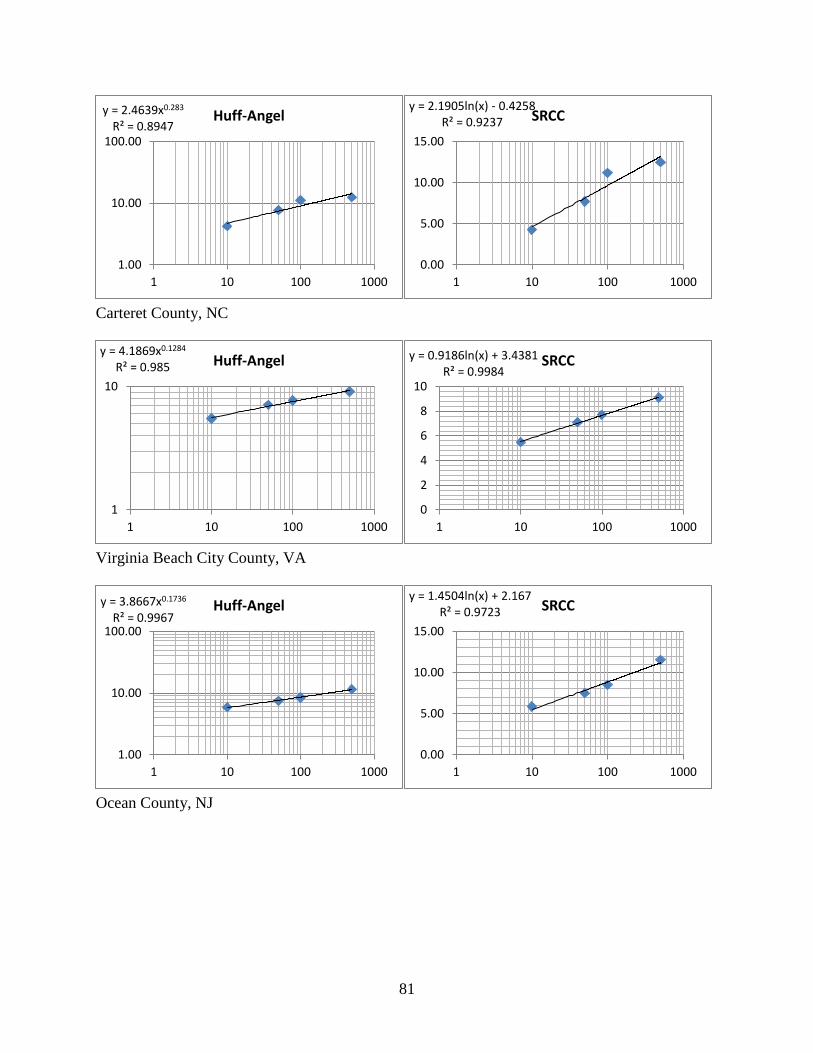
Carteret County, NC

Virginia Beach City County, VA

Ocean County, NJ

y = 2.4639x0.283 R² = 0.8947

1.00

10.00

100.00

1 10 100 1000

Huff-Angel y = 2.1905ln(x) - 0.4258

R² = 0.9237

0.00

5.00

10.00

15.00

1 10 100 1000

SRCC

y = 4.1869x0.1284 R² = 0.985

1

10

1 10 100 1000

Huff-Angel y = 0.9186ln(x) + 3.4381 R² = 0.9984

0

2

4

6

8

10

1 10 100 1000

SRCC

y = 3.8667x0.1736 R² = 0.9967

1.00

10.00

100.00

1 10 100 1000

Huff-Angel y = 1.4504ln(x) + 2.167

R² = 0.9723

0.00

5.00

10.00

15.00

1 10 100 1000

SRCC

81

Dukes County, MA

Rockingham County, NH

y = 2.6541x0.1994 R² = 0.9974

1

10

1 10 100 1000

Huff-Angel y = 1.2627ln(x) + 1.0726 R² = 0.9854

0

2

4

6

8

10

1 10 100 1000

SRCC

y = 7.5341x0.0426 R² = 0.9988

1

10

1 10 100 1000

Huff-Angel y = 0.3849ln(x) + 7.4107

R² = 0.9995

8

8.5

9

9.5

10

1 10 100 1000

SRCC

82

VITA

Frank H. Bohn was born in Galveston, Texas to Linda J. Bohn and Paul M. Bohn. Frank

has two older siblings, Kathy and David, and one younger sister, Allison. Frank graduated in the

top 3% of his senior class from Galveston Ball High School and subsequently attended Louisiana

State University. Frank graduated with a bachelor’s degree in Construction Management with

Magna Cum Laude honors. Frank began the Accelerated Master of Science program in

Engineering Science during the senior year of his undergraduate program. Frank has also

completed thirty extra hours of surveying coursework to enable him to sit for the Fundamentals

of Surveying exam. Frank has accepted a job with Vaughn Construction in Galveston, Texas,

following graduation.

83

Documents

Design flood elevations beyond code requirements and