Embed Size (px)
Citation preview

Design of a Forecasting Model for Brewing Raw Material
Consumed Price Variance
By
Adriaan van Wyk
Student no: 28327226
Submitted in partial fulfilment of the requirements for
the degree of
BACHELORS OF INDUSTRIAL ENGINEERING
in the
FACULTY OF ENGINEERING, BUILT ENVIRONMENT AND INFORMATION
TECHNOLOGY
UNIVERSITY OF PRETORIA
October 2011
Supervisor: Dr. PJ Jacobs

Executive Summary
SAB’s procurement team needs to determine expected consumed price variance (CPV) values
instead of purchased price variance (PPV) values in order to assess potential benefits of certain
business improvement projects. In this report the problem is analysed and explained and a
suggested solution is developed using Monte Carlo simulation.
The project will aim to provide SAB with a model that uses all available information to forecast
CPV for (SLM) and (HFM) for an end-of-financial-year forecasting horizon if current
operational trends are sustained. This will include an estimation of future logistics plans as
current distribution plans are only developed for a 3 month planning horizon. The model must
also be able to forecast CPV based on different strategies in order to test the potential benefit of
these strategies. The model will be able to integrate with current information systems and IT
resources that are used in Procurement.
Keywords: Brewing raw materials. Standard Lager Malt (SLM). Highly Fermentable Malt
(HFM). Consumed price variance (CPV). Purchased price variance (PPV). Procurement.
Planning. Forecast. Brewing raw materials. First-in-first-out (FIFO)

Table of Contents
1. Introduction ................................................................................................................................. 1
1.1 Problem Background ............................................................................................................ 1
1.1.1 Business Improvement Initiative ................................................................................... 1
1.1.2 Current Situation ............................................................................................................ 2
1.1.3 Brewing Raw Materials and Price Variances ................................................................ 2
1.1.4 Complexities of Malt ..................................................................................................... 5
1.2 The Problem .......................................................................................................................... 5
1.3 Summary ............................................................................................................................... 8
2. Project Aim ................................................................................................................................. 8
3. Project Scope .............................................................................................................................. 9
4. Literature Review........................................................................................................................ 9
4.1 Definition of a Forecast ........................................................................................................ 9
4.2 Selecting a forecasting method ........................................................................................... 10
5. Summary of Available Information .......................................................................................... 12
5.1 Supply Networks ................................................................................................................. 12
5.2 Data Sheets.......................................................................................................................... 14
6. Development of the Model ....................................................................................................... 15
6.1 Consolidating Data to Calculate CPV................................................................................. 15
6.2 Adding Variability to the Model ......................................................................................... 21
6.3 Summary ............................................................................................................................. 24
6.4 Model Assumptions ............................................................................................................ 25
7. Model Output ............................................................................................................................ 25

8. Model Testing ........................................................................................................................... 28
9. Conclusion ................................................................................................................................ 31
10. References ............................................................................................................................... 32
Appendix A: .................................................................................................................................. 33
South Africa Locality Map ....................................................................................................... 33
Network of Possible Supply Routes ......................................................................................... 33
Appendix B ................................................................................................................................... 34
Data Sheets................................................................................................................................ 34
DS1: Existing 3 month logistics plan.................................................................................... 34
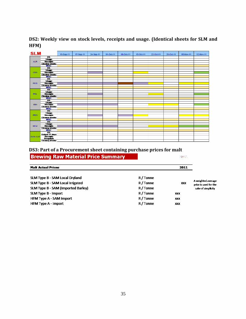
DS2: Weekly view on stock levels, receipts and usage. ....................................................... 35
DS3: Part of a Procurement sheet containing purchase prices for malt ................................ 35
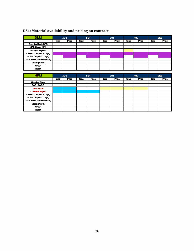
DS4: Material availability and pricing on contract ............................................................... 36
DS5: Logistics costs obtained from Procurement ................................................................. 37
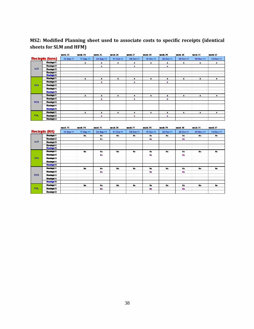
MS2: Modified Planning sheet used to associate costs to specific receipts (identical sheets
for SLM and HFM) ............................................................................................................... 38
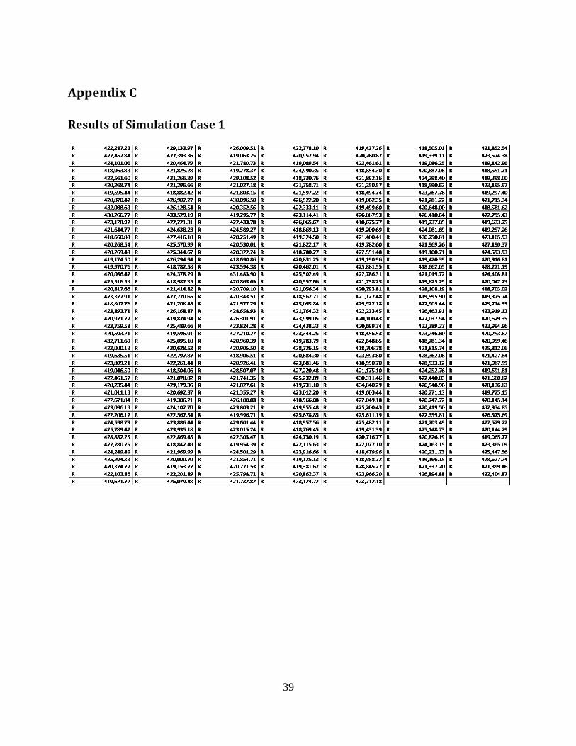
Appendix C ................................................................................................................................... 39
Results of Simulation Case 1 .................................................................................................... 39
Results of Simulation Case 2 .................................................................................................... 40

List of Figures
Figure 1: Information Flow Between Departments ........................................................................ 6
Figure 2: Current Supply Network for SLM................................................................................. 13
Figure 3: Supply Network for HFM ............................................................................................. 13
Figure 4: Information Flow Between Sheets ................................................................................ 15
Figure 5: Summary of Deliveries (MS1) ...................................................................................... 17
Figure 6: Sheet Showing Consolidated Delivery Volumes and Costs per Ton (MS2) ................. 18
Figure 7: Calculation Algorithm (MS3) ....................................................................................... 19
Figure 8: Illustration of Simulation Summary Data for a Single Brewery ................................... 20
Figure 9: Illustration of Summation of CPV per Brewery to Obtain Total CPV ......................... 21
Figure 10: Sheets Affected by Variability in Transport Lead Time ............................................. 21
Figure 11: Variable Lead Time Scenario 1 ................................................................................... 22
Figure 12: Variable Lead Time Scenario 2 ................................................................................... 22
Figure 13: Sheets Affected by Variability in Logistics Costs ....................................................... 23
Figure 14: Sheets Affected by Variability in Purchase Price ....................................................... 23
Figure 15: Sheets Affected by Variability in Weekly Material Usage ......................................... 23
Figure 16: Histogram of Simulation Output for CPV in Case 1 ................................................... 26
Figure 17: Cumulative Frequency of Simulation Output for CPV in Case 1 ............................... 26
Figure 18: Histogram of Simulation Output for CPV in Case 2 ................................................... 27
Figure 19: Cumulative Frequency of Simulation Output for CPV in Case 2 ............................... 27
Figure 20: Summary Statistics for Simulation Case 1 and Case 2 ............................................... 27
Figure 21: Mean and Standard Deviation of Transportation Lead Times .................................... 29
Figure 22: Model Test Results ...................................................................................................... 30
1
1. Introduction
* Please note that for privacy reasons some specific information related to volumes and pricing
has been replaced by “dummy” values or has been omitted from this report.
Beer is the alcoholic beverage of choice for millions of consumers worldwide. The South
African Breweries Limited (SAB) is a subsidiary of SAB Miller plc, the second largest producer
of beer in the world based on brewing volume. SAB operates seven breweries and forty depots in
South Africa and produces and imports many different brands of beer and flavoured alcoholic
beverages such as Carling Black Label, Castle, Hansa, Grolsch and Brutal Fruit among others.
In order to maintain the meeting of an enormous demand and brewing volume thorough supply
chain planning and management is required. These activities are mainly undertaken by the
planning department (Planning), dealing with activities such as demand planning and brewing
plans for the seven different breweries, and the procurement department (Procurement), dealing
with the identification of suppliers and negotiating supplier contracts and ensuring that any
product or commodity that SAB purchases gets delivered at the right time, place, price and
quantity.
1.1 Problem Background
1.1.1 Business Improvement Initiative
As from the beginning of this year Procurement has been running a major initiative to
optimise the value Procurement delivers annually. A target of R220 million and a stretch
target of R300 million in savings within the next year has been set. These are all savings that
should result from projects relating to improvement of operations, negotiations with
suppliers, cutting of unnecessary cost, innovation, i.e. from doing business more
efficiently and more economically.
In order to meet such targets the benefit for every project must be reported. This implies that
business benefit arising from a project must be measurable and traceable in order to compare
2
realised benefit with original targeted benefit. More specifically benefit must be determinable
relating to the following:
Targeted benefit of the project must be proven to be realistic before a project can be
approved
Actual realised benefit must be reported during the lifetime of the project on a periodic
basis
As the project progresses and more information becomes available the expected final
benefit must be adjusted accordingly
Final benefit delivered must be accurately reported upon completion of the project.
1.1.2 Current Situation
SAB has comprehensive and effective information systems in place for reporting on past
activities, mostly by means of SAP. The way future operations are predicted however depends
largely on the department, the specific operation within the department or the specific project.
Expected values of operational variables are mostly obtained by using and manipulating values
from operational plans or values based on contracts signed with suppliers. In general, if there is a
lot of variation in a variable for which a future value has to be determined or no plan exists for
the timeframe within which it should be determined, no prediction is done as is the case for
certain variables relating to brewing raw material usage.
1.1.3 Brewing Raw Materials and Price Variances
The Procurement team handling operations relating to brewing raw materials makes use of price
variances as a means of measuring certain benefits.
According to Seal et al, in management accounting price variances are differences between
actual prices and standard prices where standard prices are used to set up budgets.
Two price variances are highlighted. Variance in purchase price is referred to as purchased price
variance (PPV) and is calculated as the difference between the budget for raw material purchases
and actual cost of the same volume of raw material for SAB as a whole. PPV for a specific
purchase of raw material is calculated as

3
Where
PV = Purchased Volume
BR = Budgeted Rate
AR = Actual Rate.
It then follows logically that PPV for a certain time period is calculated as
Where T =Set including all purchases in considered time period.
It includes all material costs and logistics costs up to the point that the relevant SAB brewery
takes control of the material. A system for calculating PPV based on historical operations is in
place. Expected PPV is also determined very accurately as contracts are signed with suppliers for
raw material shipments months ahead. The main reason for the lack of accuracy that does exist is
averaging values used for logistics cost to breweries; a standard rate per ton is allocated to each
brewery for inland logistics costs irrespective of the actual route the material takes. PPV is
mainly used to determine benefit relating material purchases at newly negotiated prices; however
it is also influenced by certain other factors such as variability in actual shipping times for
imports.
Variance in the price of consumed raw materials is referred to as consumed price variance
(CPV). Its calculation is similar to that of PPV, also including all logistics and storage costs up to
the point where the material is delivered to the brewery. The difference is the timing of when the
cost is allocated to the material. For CPV at a certain point in time (CPVt):
Where CU = Cost of purchased but unconsumed material.
The cost of unconsumed material includes all material that SAB has taken ownership of i.e.
imports delivered to the harbour (depending on Incoterms negotiated with supplier) and material

4
made available to SAB by local suppliers. Associated cost to unconsumed material includes
material costs and logistics costs up to the point that the relevant SAB brewery takes control of
the material whether or not the cost has already been incurred of will be incurred in the future.
CPV is more complex to determine due to the fact that material is used at a brewery level and
needs to be computed for each brewery for each time interval (e.g. each week) before a total
SAB view can be established. I.e. average values for inland logistics are not sufficient and inland
logistics cost must be associated to each material delivery individually. For most raw materials
however supplier and logistics networks are fairly straightforward and constant. This fact
combined with the fact that purchase prices remain constant during a contract period makes it
possible to obtain a high level view of such CPV values for a certain raw material for a contract
period by using material usage values based on Planning’s production values, material costs and
logistics costs:
Where
B = Set Containing Referring to All Breweries
MN = Material Need
PP = Purchase Price
LC = Total Inland Logistics Cost
The “Budgeted Rate” includes purchase price and logistics cost.
Although all the necessary information to calculate CPV values is recorded during several
different Planning and Procurement activities, no system exists that can consolidate the
information and calculate CPV values.

5
1.1.4 Complexities of Malt
The level of complexity rises when finding CPV for the main raw material, malt, which includes
standard lager malt (SLM) and highly fermentable malt (HFM), for the following reasons:
Both imported and locally produced malt is used and their prices differ
There exists no fixed ratio as to what type of malt (import or local) a brewery receives.
There exists no fixed ratio according to which imported or locally produced malt is mixed
in a certain brew i.e. they are interchangeable.
Consequently the effective price of consumed malt is not constant over a certain period
and the equation above cannot be used to estimate future CPV values for malt
Specifically relating to future or expected CPV values, distribution for malt deliveries to
breweries is only planned three months in advance.
Based on the last point the current tendency to manipulate planned values to estimate future
values cannot be used to find expected CPV values for more than 3 months in advance.
1.2 The Problem
Currently retrospective and expected PPV values can be calculated adequately. Procurement
however wishes to start making use of CPV instead of PPV in order to measure benefits relating
to certain products and certain materials. As the previous paragraphs suggest, this cannot be done
with current systems.
In order to gain a better understanding of the problem to be solved it is necessary to acquire more
insight on how information flows between Planning and Procurement functions. The process for
malt will be discussed as it is the focus of this report (as stated under the discussion of the project
scope). It is however noteworthy that the processes for other raw materials are similar to that of
malt even though there may be some simplifications. Consider the flow diagram below (Figure
1).

6
Demand
Forecast
Volume
Planning
Material
Requirements
Planning
Negotiate
Suppliers
Planning Procurement
Local Malt
Production
Schedule
Imports
Schedule
Logistics
Plan
Arrange Fleet
(Internal or
External
Suppliers are
Used)
Figure 1: Information Flow Between Departments
At the end of a financial year Planning forecasts demand for all brands for 3 years in
advance.
Based on this forecast brewing planning or volume planning is done: Weekly brewing
plans are formulated for the period until the end of the next financial year for all 7
breweries.
Based on each brand’s malt requirements and brewing volumes overall malt requirements
are determined.
Procurement sources malt from local and international malt producers.
As a result of Procurement’s negotiations with suppliers a schedule of available malt
from local suppliers and imported malt to arrive at the harbour is created. This shows
availability on a weekly basis.
Planning uses the knowledge on malt availability and production plans for breweries in
conjunction with feedback from breweries on available storage space to prepare a
logistics plan. The logistics plan is fixed for the following month’s malt transport and a
tentative plan is prepared for the next two months in advance.

7
Procurement arranges fleets to accommodate the logistics plan.
Malt is transported to the breweries where the malt is consumed.
It is clear that Procurement is responsible for the large cost incurring activities of SAB which
relate to materials, such as raw material purchases or arrangement with logistics contractors.
Which costs to assign to specific volumes of material existing in different phases of the supply
chain are however influenced by information from both departments. Due to the level at which
SAB calculates PPV, it is possible for Procurement to calculate PPV using information that they
primarily govern. CPV however is dependant on the specific logistical route a specific volume of
material takes before being consumed at a specific brewery. This means that cost information
from Procurement, logistics information from Planning and brewery specific volume information
from Planning is necessary for calculating CPV. This means that a large part the problem is
scattered information which needs to be consolidated before CPV can be calculated.
This however raises the question on whether it is an information management problem, or
whether it is indeed also a forecasting problem. It is evident that Planning’s original demand
forecast is an input to volume plans, which determines the volumes that Procurement sources,
both which influence logistics. The last three aspects mentioned all in turn influence CPV, in
fact, if costing aspects are included the aforementioned list it includes all the primary inputs that
influence CPV. Hence a forecast of a financial year’s CPV would indirectly be driven by the first
forecast of demand. If the relevant information based on the first forecast is available and can be
processed in such a way as to obtain the expected CPV, is the expected CPV a forecast in its own
right? Linking back to the briefly discussed aspect of variability in future variables, would the
expected CPV calculation be a forecast in its own right if it takes into account possible
variability on the relevant information? At this point it becomes necessary to consult the
literature.

8
1.3 Summary
SAB’s Procurement team in charge of brewing raw materials cannot verify savings opportunities
relating to the price of consumed raw materials as no forecast for CPV exists and consequently
the potential effect of improvement initiatives relating thereto cannot be forecasted. A forecast
using currently implemented methods and systems cannot be done due to the following facts:
Necessary information is scattered between departments and needs to be consolidated in
some way.
No current systems can take into account possible variability of future variables when
determining expected values.
A distribution plan for the required forecasting horizon does not exist.
2. Project Aim
The aim of this project is to design a model that can consolidate the available information from
the relevant departments (inputs) and process it to deliver an expected CPV value, based on
current operational trends, for the forecasting horizon (output) using available information. It
must also be able to take different operational variables based on different strategies as input and
forecast CPV based on these strategies in order to test them. The model will be compatible with
current information systems that are used – mainly meaning that it must not be necessary to
purchase new software. An estimation of logistics plans for an end-of-financial year planning
horizon will be generated and input to the model that will extend the forecasting horizon. The
logistics plan must be approved by planning in order to ensure that it will resemble actual future
distribution as accurately as possible. The model will account for variability in planned values in
order to provide the most accurately achievable output.

9
3. Project Scope
Based on Procurement needs from the model as expressed by its representative’s and available
time for project completion, the following boundaries have been established
As HMF and SLM are the main raw materials used, the project will include a distribution
plan and forecasts of CPV for only both major types of malt, SLM and HFM, for all 7
breweries for the next 12 months. The model may be adapted or simplified to
accommodate other raw materials at a later stage.
It will not include planning of demand or planning of production but rather assume that
available plans are satisfactory and take it as input to the model.
4. Literature Review
4.1 Definition of a Forecast
The question on whether the determining of future CPV values is a forecast by its own right
needs to be addressed.
Many different opinions exist in the literature regarding the strict definition of a forecast,
especially when it is compared to another concept referred to as a prediction. (Freeman et al.
1979, p. 114). Some use the terms interchangeably or make no precise distinctions (Zarnowitz,
1968: 425) or (Theil, 1971). Others regard forecasts and predictions as distinct activities, but
differ on the nature of the distinction, e.g. for one forecasts would be a subset of predictions and
for another it would be the other way around. (Schuessler 1968: 418), (Choucri 1974: 63).
Another opinion is that a forecast is a weaker activity due to a prediction being deductive and a
forecast being inductive in nature, making a forecast less reliable (Hempel, 1965). Freeman et al
(1979, p.117) attempts to clarify this in the following way: It is suggested that forecasts and
predictions have 3 aspects in common namely that in general a relationship exists between
certain outcomes under certain conditions, a claim that these conditions will exist at a certain
future time, and a statement on the probability of certain outcomes happening at said future time
under said conditions. If the statement on the probability of certain outcomes is based on the

10
generalization of the relationship between the outcomes and certain conditions and the claim that
the conditions will definitely occur, Freeman et al classifies it as a prediction. If the statement on
probabilities is however based on generalization of the relationship between the outcomes and
certain conditions and the claim that the conditions will occur based on some stated probability,
then it is classified as a forecast.
The calculation of expected CPV adheres to the 3 aspects that are common to predictions and
forecasts, however certain inputs such as material usage (discussed under the Method section),
define certain circumstances with certain probability distributions. This implies that according to
the suggested classification by Freeman et al the determining of future CPV values is in this case
a forecast, which implies that it is a forecast by its own right.
4.2 Selecting a forecasting method
This project requires forecasting of raw material usage and raw material prices to forecast
consumed price variance. Gentry et al. (2006, p56) suggested a way to classify forecasting
methods based on two main factors, judgemental methods and empirical evaluated ideas, and
naive and causal forecasting. The result was classification of methods as correlations, models,
predictions and scripts. Correlations are forecasts based on performance of another factor,
without making any causal assumptions and include methods such as extrapolation, analogies,
and neural networks. Models are forecasts based on specific causal assumptions that can be
described by mathematics and include methods such as expert systems, econometric models, and
structural models. Predictions, as the name suggests, are speculated outcomes based on no
specific causal assumptions and includes the Delphi method, conjoint analysis, and expert
opinion. Scripts are speculative forecasts based on specific causal assumptions and include
methods such as role playing, scenarios and traditional writings.
This forecast is based on causal assumptions such as a raw material distribution plan that will
greatly influence when malt will be delivered and used at breweries. For this reason Predictions
and Correlations as defined by Gentry can be ruled out.
11
Under the Models class expert systems use rules that experts use to make a forecast (Armstrong,
2001). Although certain expert opinions influence the inputs to the model, many calculations are
needed that account for variability, ruling out expert systems. According to Gentry (p12)
econometric models usually refer to regression models, which is also not a fit. Structural models
“simulate the impact of important causal factors”. Forrester (1958). Gentry’s summary of
Forrester does however not explicitly state whether this will provide the needed quantitative
analysis.
Under the Scripts class role-playing makes use of subjects acting in certain roles in order to
predict behaviour which is irrelevant in this case. Traditional writings aren’t a match for self-
explanatory reasons. According to Bright (1978) scenarios describe all possible future events in
detail and use them to decide on what actions to take. This does not provide the qualitative
output that is required.
Another option does however exist in the world of risk analysis. According to Evans (2010,
p349) risk is the probability of occurrence of an undesirable outcome. Risk analysis techniques
consider certain risks which by definition are events that have a probability of happening in the
future. Inherent to risk analysis then is the making of predictions or forecast on the risk events on
which risk managing decisions can be made. These techniques can be applied to other outcomes
that may or may not be risk events in order to make predictions or forecasts thereon. As an
example Evans explicitly refers to the output of a Monte Carlo simulation (which is a risk
analysis technique) as forecasts. (Evans, 2010, p357). Also on p349; “Monte Carlo simulation is
the process of repeatedly generating inputs to a decision model based on sampling from their
assumed probability distributions, calculating the outputs and analyzing the results. Of particular
interest are the distributions of the output variables, which characterize the likelihood that certain
output values will be achieved.” This technique can be tailored to take assumed distributions of
model inputs such as logistics plan’s delivery dates, raw material usage or prices, apply the
model to the inputs and generate probability distributions for the outputs. This method can fall
under the Models category of Gentry’s classification grid due to it producing a forecast by taking
certain explicitly defined causal assumptions that can be described mathematically as input and
processes it to produce a forecast as output. Monte Carlo simulation also adheres to the aims of

12
the model for use in with the project namely that it can produce a forecast, it can be modelled
with readily available software such as spreadsheets and it can take into account a lot of
variability. For these reasons it will be the method of choice for this project.
5. Summary of Available Information
5.1 Supply Networks
The first piece of relevant information to discuss is the supply networks used to transport malt
from suppliers to breweries as the cost elements that relate to it summarises to one of the primary
factors that makes the required CPV values more complex to calculate than the current PPV
values. It also supports the understanding of the gathered input data that is to follow and how
distribution planning is done. A map showing different site’s approximate geographical positions
in South Africa has been added in Appendix A in order to aid in the visualisation of the supply
networks. This would also help clarify certain practical issues and constraints that drive supply
networks. A diagram illustrating all optional supply routes, all that have been used in the past,
has also been added in Appendix A.
Below are two diagrams illustrating currently used supply networks, one describing SLM supply
and the other describing HFM supply. These describe routes and transport modes that are
currently used and will be used for the foreseeable future. Each route and associated transport
mode has a cost associated with its usage.
Note that currently all SLM is locally sourced and all HFM is imported. It is also worthy to
mention that the intermediate storage capacity of Premier is avoided as it incurs extra cost. Also
noteworthy is that both “bulk” and “containers” are imported by ship and transported inland by
either rail or road depending on the specific link hence a single rate is used for each link.

13
Alrode
Maltings
Caledon
Maltings
Alrode
Chamdor
Ibhayi
Newlands
Polokwane
Rosslyn
Road
Rail
Road
Rail
Rail
Rail
Rai
l
Premier
Rai
l
Cape Town
HarbourDurban
HarbourSea
Prospecton
RoadRoad
Brewery
Optional Intermediate Storage
xxxxxx Transport Mode
Harbour
Supplier
Figure 2: Current Supply Network for SLM
Imported Malt
Alrode
Chamdor
Ibhayi
Newlands
Polokwane
Rosslyn
Premier
Bulk
Bul
k
Prospecton
Durban
Harbour
Bulk
Bulk
Containers
Containers
Bulk
Bulk
Brewery
Optional Intermediate Storage
xxxxxx Transport Mode
Harbour
Supplier
Port Elizabeth
Harbour
Port Elizabeth
Harbour
Figure 3: Supply Network for HFM

14
5.2 Data Sheets
Examples of actual sheets maintained by Planning and Procurement persons have been added
Appendix B. In summary they include:
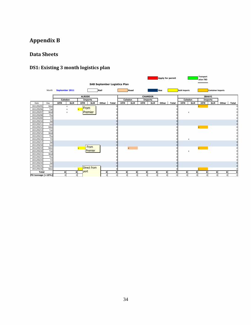
DS1: Existing 3 month logistics plan. This sheet contains the logistics plan that has been
discussed earlier in this report. Planned dispatches of SLM from local producers (Caledon and
Alrode) are tabulated under the SLM heading for each brewery. Note that Premier’s storage is
only used for imported malt in cases where problems occur and is as a rule not currently used.
Planned imports to each brewery are given under the HFM heading and a colour code system is
used to indicate transport mode. Imports dispatches for Newlands, Prospecton and Ibhayi will
always be directly from the closest harbour. Import dispatches to the other four breweries will
mostly be from premier. This is due to the fact that malt is imported in very large volumes to
enable negotiating of a better price. In some cases imports do however get transported directly
from Durban harbour to one of the aforementioned four the breweries. The specific link used is
indicated on the Planning sheet using a “note” (see DS1) and inland logistics costs need to be
allocated accordingly.
DS2: Weekly view on stock levels, receipts and usage. This sheet contains planned malt usages
that have already been calculated based on Planning’s weekly production schedule. It also
contains the sum of each specific week’s planned receipts at breweries based on the logistics
plan, manually entered by Planning.
DS3: Part of a Procurement sheet containing purchase prices for malt. Sheet added for
illustrative purposes.
DS4: Material availability and pricing on contract. This contains Planning’s version of the
schedule of available materials for purchases. DS4 shows the modified version of this sheet that
the model uses to accommodate related purchase prices explained in the next section.
DS5: Logistics costs obtained from Procurement. This sheet contains contracted costs of
moving malt through different links in the supply network.

15
6. Development of the Model
In order to solve Procurement’s problem, the aforementioned data must be consolidated and used
to forecast CPV. The data is available in Excel sheets and as Excel can be used quite effectively
to generate random numbers used in Monte Carlo simulations. Based on the latter and the fact
that part of the aim of the project is to develop a model that is compatible with currently used
systems, Excel will be used to implement the model.
6.1 Consolidating Data to Calculate CPV
Consider the diagram below depicting information flow between data sheets and the model
(which will also be built in Excel sheets as discussed).
DS1:
Logistics
plan
DS2:
Weekly
receipts and
usage
Volume
plans
Material
needs per
brand
Material
requirements
plan
DS3:
Brewing
raw material
price
summary
DS4:
Contracted
purchase
prices per
month
DS5:
Contracted
logistics
costsMS 2: Cost
per receipt
MS3: CPV
Calculation
Algorithm
MS4: Forecast
(Monte Carlo
simulation
sheets)
MS5:
Forecast
results
Weekly usage
Model
MS1:
Deliveries
Summary
Dispatches
Receipts
Figure 4: Information Flow Between Sheets
16
For the sake of clarity on where planned usage values originates from the flow from volume
planning and material needs per brand into a material requirements plan which flows into DS2
has been indicated. This is however a piece of work that is already done by Planning for the
desired forecasting horizon and will not be repeated in this project.
DS1-DS2: It is however worth mentioning that the logistics plans from DS1 determine
the receipts of DS2: The lead time needs to be added to the dispatch date according to the
logistics plans in order to obtain the receipt date. The sums of all resulting receipts per
week are documented in DS2. The implication of the fact that the sums of receipts are
entered is that it is not possible to associate costs to the receipts accurately. It is needed to
observe each delivery to each brewery and its associated cost individually in order to
track costs accurately and compute CPV. Note that the way in which the information is
presented in this sheet using colour codes and notes makes it difficult to pull through to
different sheets using simple cell references.
(DS1 and DS5)-MS1: The first model sheet, Deliveries Summary, is made necessary by
the manual means by which logistics plans are generated and entered into worksheets. It
is necessary to process this information manually in order to make it more usable in
Excel and make the rest of the model more user-friendly. MS1 Contains a summary of all
dispatches times, dispatch volumes, lead times, expected receipt dates, transport routes
and resulting logistics costs for every expected receipt. This sheet is then used to view
individual receipts and allocate costs to them as discussed above.
The bit of work around adding lead times to dispatch times to obtain receipt times is
already done by planning in order to compile its stock summary in DS2, it is simply not
noted down. It follows logically that if MS1’s receipts are summated over each week, it
should equal the receipts of DS2. This can be used to test MS1’s values against
planning’s values before variability is analysed (see discussion on adding variability to
the model).

17
Figure 5: Summary of Deliveries (MS1)
DS3-DS4: The modified sheet referred to as DS4 is used to summarise contracted
purchase price information on a monthly basis which are obtained from Procurement’s
pricing sheets, part of which is illustrated in DS3. This information is entered manually
when supplier contracts are negotiated and confirmed when contracts are confirmed.
(DS4 and MS1)-MS2: MS2 is used to summarize all incurred costs relating each specific
receipt. Thanks to the bit of work done in MS1, MS2 automatically pulls the individual
receipts and their costs into sheets that can be used to as input to a CPV calculation.
MS2 – Individual Receipts and Costs: Modified Planning sheet used to associate costs to
specific receipts (identical sheets for SLM and HFM). Used for data consolidation,
specifically adding material costs and logistics costs for each receipt.
18
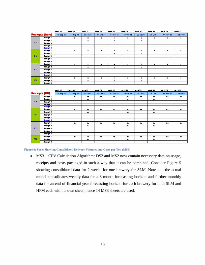
Figure 6: Sheet Showing Consolidated Delivery Volumes and Costs per Ton (MS2)
MS3 – CPV Calculation Algorithm: DS2 and MS2 now contain necessary data on usage,
receipts and costs packaged in such a way that it can be combined. Consider Figure 5
showing consolidated data for 2 weeks for one brewery for SLM. Note that the actual
model consolidates weekly data for a 3 month forecasting horizon and further monthly
data for an end-of-financial year forecasting horizon for each brewery for both SLM and
HFM each with its own sheet, hence 14 MS3 sheets are used.

19
Figure 7: Calculation Algorithm (MS3)
This sheet automatically pulls information from DS2 and MS2 for each week (or month)
into the highlighted cells. To the left of the highlighted cells it shows the opening stock
for the week (and consequently closing stock for the previous week) in order of original
delivery. To the right of the highlighted cells it shows the results of the model’s
calculation on how the material will be used in a first-in-first-out basis (see model
assumptions). To the right of “FIFO Usage” it uses the prices pulled from MS2 to
calculate the forecasted cost of consumed material. Note that the size of the sheet i.e. the
number of receipts in opening stock and number of new deliveries it tracks is dependent
on the specific brewery and material.
This sheet consequently not only consolidates data, but also generates a possible future
scenario. It can therefore also used to impose probability distributions any of the
variables it contains, such as “Total usage”, or “Price” if the specific price has not been
fixed by a contract yet. (See discussion on adding variability to the model)
MS4: In the forecasting part of the model a Monte Carlo simulation is done on each of
the 14 “consolidation sheets”; Excel’s “What If Analysis” (more on this when under
section discussing variability) is used to generate many possible scenarios giving many

20
possible CPV values, the summarising statistics of which gives the forecast price of
consumed material. It also effectively gives a probability distribution for the CPV value
which can be used in decision making when alternative strategies are considered.
Note that each simulation is run in a separate Excel workbook that pulls the information
on usage and distributions from the MS3 sheets. This is done in order to have a level of
control over when certain computations are done by the computer to avoid crashing – a
single workbook containing a simulation can be opened, updated and closed again before
the next is opened.
MS5: Each of the aforementioned workbooks summarises simulation data and calculates
weekly CPV as illustrated in Figure 6. Note that standard costs are pulled from
Procurement’s “Standard Costs” sheet.
Figure 8: Illustration of Simulation Summary Data for a Single Brewery
Summary data from the 14 simulation workbooks get pulled back to the original
workbook where total CPV is calculated. See Figure 7.

21
Figure 9: Illustration of Summation of CPV per Brewery to Obtain Total CPV
6.2 Adding Variability to the Model
Note that the above sheets as described only calculate a possible scenario of weekly CPV values
based on expected or planned values. The advantage however of having Excel automatically read
and calculate values from input sheets is that should a value in an input cell be replaced with a
random number that excel generates, the dependent cells in the subsequent sheets automatically
reads the newly generated value and recalculates its own value. If such a random value generated
by Excel is used for certain inputs the effect is that the model calculates a new possible scenario
of CPV values each time new random values are generated. The model specifically enables
adding variability to the following:
Transport Lead Times (MS1)
For the sake of aiding in the visualisation of how values would change in sheets an example
using screenshots focussing on changing values is given for transport lead times.
Consider the diagrams below illustrating two scenarios based on random numbers generated for
lead times and the effect it has on the rest of the model.
MS 2: Cost
per receipt
MS3: CPV
Calculation
Algorithm
MS1:
Deliveries
Summary
Receipts
Figure 10: Sheets Affected by Variability in Transport Lead Time

22
Figure 11: Variable Lead Time Scenario 1
Figure 12: Variable Lead Time Scenario 2
23
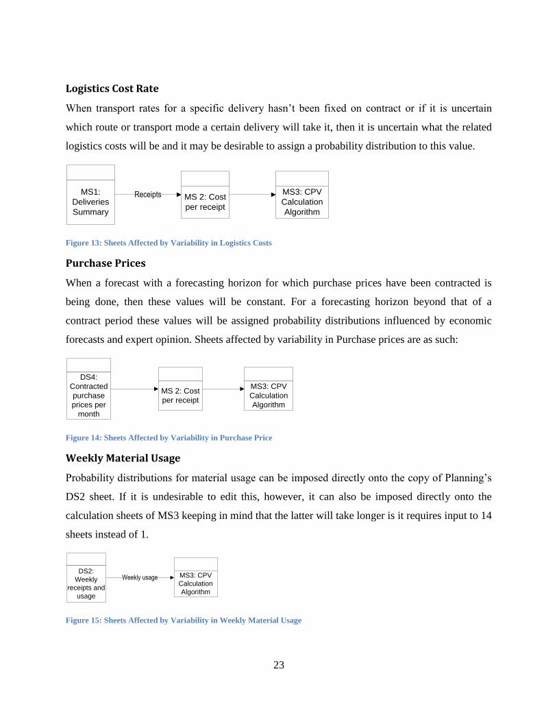
Logistics Cost Rate
When transport rates for a specific delivery hasn’t been fixed on contract or if it is uncertain
which route or transport mode a certain delivery will take it, then it is uncertain what the related
logistics costs will be and it may be desirable to assign a probability distribution to this value.
MS 2: Cost
per receipt
MS3: CPV
Calculation
Algorithm
MS1:
Deliveries
Summary
Receipts
Figure 13: Sheets Affected by Variability in Logistics Costs
Purchase Prices
When a forecast with a forecasting horizon for which purchase prices have been contracted is
being done, then these values will be constant. For a forecasting horizon beyond that of a
contract period these values will be assigned probability distributions influenced by economic
forecasts and expert opinion. Sheets affected by variability in Purchase prices are as such:
DS4:
Contracted
purchase
prices per
month
MS 2: Cost
per receipt
MS3: CPV
Calculation
Algorithm
Figure 14: Sheets Affected by Variability in Purchase Price
Weekly Material Usage
Probability distributions for material usage can be imposed directly onto the copy of Planning’s
DS2 sheet. If it is undesirable to edit this, however, it can also be imposed directly onto the
calculation sheets of MS3 keeping in mind that the latter will take longer is it requires input to 14
sheets instead of 1.
DS2:
Weekly
receipts and
usage
MS3: CPV
Calculation
Algorithm
Weekly usage
Figure 15: Sheets Affected by Variability in Weekly Material Usage

24
Business or Process Rules
It is necessary to note at this point that not only variability in inputs can be imposed on these
sheets, but also business rules affecting model values. The summation of stock items and the
adjustment of planned usage values according variation between actual and planned usage (see
model assumptions) are examples of such rules.
Summarising Many Generated Scenarios
It is now clear that the model can generate a possible scenario for values contributing to CPV
based on expected values. It can also generate many more possible scenarios based on variable
inputs, created by assigning values generated from probability distributions to the variables.
However, it would be impractical to manually command Excel to generate new scenarios and
manually note down these values for summarising.
Excel provides a practical solution that it calls “What-If Analysis”. When using this function,
one selects a cell in a worksheet for Excel to analyse. Excel takes into account all other formulae
and cells that influences the selected cell’s value and automatically generates as many different
possible values for this cell as it is commanded to. For this model the total cost of consumed
material or “Consumed Price” is used, however, it should be noted that it can be used to analyse
consumed prices for any or all weeks, for usage values, stock levels etc.
6.3 Summary
The largest bit of manual work when using the model is the completion of MS1. The rest simply
includes addition of material prices (and pricing probability distributions) in MS2, copying
Planning’s DS2 sheet into the model (and imposing probability distributions if necessary) and
then the model automatically runs Monte Carlo simulations on the sheets of MS4 when the are
opened and closed and results are summarised in MS5.
Currently results are total CPV values for September 2011 to March 2012, but model can be
adapted to give different information if necessary.
25
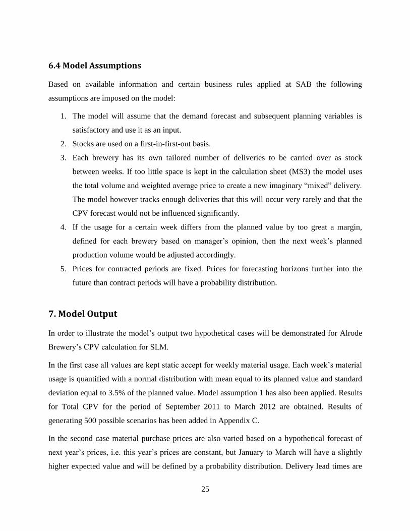
6.4 Model Assumptions
Based on available information and certain business rules applied at SAB the following
assumptions are imposed on the model:
1. The model will assume that the demand forecast and subsequent planning variables is
satisfactory and use it as an input.
2. Stocks are used on a first-in-first-out basis.
3. Each brewery has its own tailored number of deliveries to be carried over as stock
between weeks. If too little space is kept in the calculation sheet (MS3) the model uses
the total volume and weighted average price to create a new imaginary “mixed” delivery.
The model however tracks enough deliveries that this will occur very rarely and that the
CPV forecast would not be influenced significantly.
4. If the usage for a certain week differs from the planned value by too great a margin,
defined for each brewery based on manager’s opinion, then the next week’s planned
production volume would be adjusted accordingly.
5. Prices for contracted periods are fixed. Prices for forecasting horizons further into the
future than contract periods will have a probability distribution.
7. Model Output
In order to illustrate the model’s output two hypothetical cases will be demonstrated for Alrode
Brewery’s CPV calculation for SLM.
In the first case all values are kept static accept for weekly material usage. Each week’s material
usage is quantified with a normal distribution with mean equal to its planned value and standard
deviation equal to 3.5% of the planned value. Model assumption 1 has also been applied. Results
for Total CPV for the period of September 2011 to March 2012 are obtained. Results of
generating 500 possible scenarios has been added in Appendix C.
In the second case material purchase prices are also varied based on a hypothetical forecast of
next year’s prices, i.e. this year’s prices are constant, but January to March will have a slightly
higher expected value and will be defined by a probability distribution. Delivery lead times are
26
varied. Variable weekly usage and assumption 4 is imposed as in the first case. Results of
generating 500 possible scenarios has been added in Appendix C.
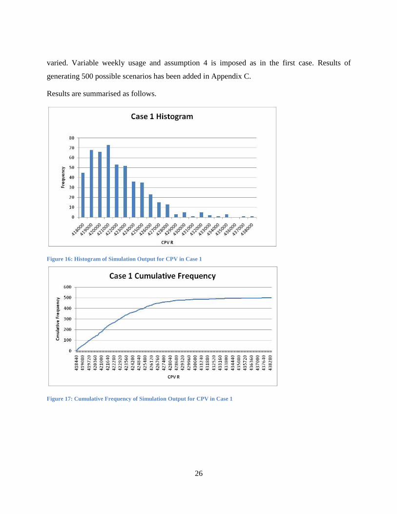
Results are summarised as follows.
Figure 16: Histogram of Simulation Output for CPV in Case 1
Figure 17: Cumulative Frequency of Simulation Output for CPV in Case 1

27
Figure 18: Histogram of Simulation Output for CPV in Case 2
Figure 19: Cumulative Frequency of Simulation Output for CPV in Case 2
Figure 20: Summary Statistics for Simulation Case 1 and Case 2

28
Case 1 shows that the total CPV for the forecasting period would be between R 418 455.93 and
R 438 449.45 with an expected value of R 422 570.09. The small range implies that the model
does not describe a lot of variability and CPV can be forecasted very accurately. This is due to
the fact that in case 1 only usage is variable whereas in reality other inputs would also be
variable. The business rule that adapts a week’s planned usage values according to the variation
in the previous week’s usage also causes total usage for the forecasting period to lean towards
the planned value and this reduces variability further. The value is also very optimistic because it
doesn’t take into account possible price changes in 2012.
Case 2 shows an expected total CPV of R 146 641.54, but indicates that it can still be expected
that the actual value will fall between R 48 387.22 and R 234 547.20. The wider range indicates
the larger uncertainty that arises due to the fact the variability in purchase price is taken into
account. The smaller expected value is caused by the fact that possible price increases is
considered when the probability distribution of 2012 purchase prices are determined.
Depending on the decisions to be made, other analysis can also be done with the data such as the
probability that CPV would be larger or smaller than a critical value or the probability that it
would fall between certain critical values.
8. Model Testing
The information that the model can process and the variability that it can take into account when
making a forecast has been discussed. Before using the model’s output to base real decisions on
it is necessary to test its validity. This has been done in the following way - Please note that
although the model currently has the capability to forecast CPV for all breweries, not all input
data is currently available as different breweries keep different records. Due to availability of
data Alrode is used to test the model: Input data as described above exists for historical
operations as from beginning April 2011 to end August 2011. This information was used as input
to the model and a Total CPV forecast for the period April 2011 to August 2011 was generated.
More specifically:

29
Logistics plans with dispatch dates: Latest versions of each month’s logistics plans were
used.
Transport lead times: Normal distributions with mean lead times and standard deviations
based on figure 21, used by Planning, were implemented when running the simulation.
For transportation links where no information is available static values were used.
Logistics cost rate: Contracts for the relevant period were fixed. Logistics cost values
were however scaled according to the lead time of a generated scenario to account for
costs incurred (or saved) by long or short lead times.
Purchase prices: Contracts for the relevant period were fixed and static values were used
in the simulation.
Weekly material usage: Varied according to Alrode’s operations manager’s analysis of
variation between planned and actual production. Model assumption 4 was imposed.
Figure 21: Mean and Standard Deviation of Transportation Lead Times
Actual values:
Actual production values for April to August, drawn from SAP, is multiplied by the
standard rate for Alrode to obtain each month’s standard cost.

30
Actual material cost values for April to August, also drawn from SAP, is subtracted from
each month’s standard cost in order to obtain actual CPV for April to August.
The relation between forecast CPV and actual CPV is used to test the model’s validity.
As actual volume and cost values can’t be included in this report the percentage difference
between each month’s actual and forecast values used in this analysis:
Figure 22: Model Test Results
According to this analysis one can expect that, for any month, the forecast would be within
14.11% of the actual CPV and for a total CPV with a 5 month forecasting horizon one can expect
the forecast CPV to be about 9% accurate. It is necessary to note that this analysis was done
using actual logistics plans from Planning which were available as historical values were used;
hence the estimation of logistics plans for a beyond-3 month forecasting horizon was not
necessary as it would be for an actual forecast. One can thus expect that the results from this
analysis would apply to a forecast with a 3-month forecasting horizon and that forecasts for the
successive months will be less accurate.
31
9. Conclusion
Procurement needs a CPV forecast in order to determine potential benefits of certain projects.
The literature has been consulted and it has been established that it is possible to solve. A model
has been developed that consolidates information influencing CPV values and applied Monte
Carlo simulation to forecast these values.
The model can also accommodate many different inputs and can apply variability to all values it
describes and for this reason it can be used to forecast CPV for many different strategies based
on many different assumptions (as partly illustrated in the model output section).
With only slight modifications, the model cab analyse other aspects such as stock levels based on
given inputs and assumptions. More specifically it numerically defines probability distributions
for all these outputs. This can aid in decision making when considering different strategies.
When applying the model to the current trends it is expected to give 9% accurate forecasts for a
forecasting horizon smaller than three months, but less accurate for a longer forecasting horizon.
This is due to the uncertainty caused by the fact the logistics plans are only generated for a three
month planning horizon.
It can be recommended that a joint initiative between Planning and Procurement be started to
lengthen the logistics planning horizon in order to be able to generate better forecasts for longer
forecasting horizons. This can be included in the strategies that the model will test.
The next step would be to use the actual model to test strategies such as using different transport
modes or routes, using more or less intermediate storage or keeping more or less stock.
An interesting addition to the model would be to take into account holding cost of stock at
breweries and revisit current and optional strategies.

32
10. References
Armstrong, J. S. (2001). Principles Of Forecasting: A Handbook For Researchers And
Practitioners. Boston: Kluwer Academic Publishers.
Choucri, N. (1974) "Forecasting in international relations: problems and prospects." International
Transactions 1: 63-86.
Evans, R.J. (2010) Statistics, Data Analysis and Decision Modeling, 4th
ed., Pearson, New Jersey.
Forrester, J. W. (1958). Industrial Dynamics: A Major Breakthrough For Decision Makers.
Harvard Business Review, 36, 37-66.
Freeman J.R. and Job B.L. (1979) Scientific Forecasts in International Relations: Problems of
Definition and Epistemology, International Studies Quarterly, Volume23(1), p. 113-143.
last accessed 12/09/2011, from http://www.jstor.org/stable/2600276.
Gentry, l., R. Calantone., Cui, S.A., 2006. The forecasting classification grid: A typology for
method
selection. J Global Bus. Manage., 2: 48-60
Hempel, C. (1965) Aspects of Scientific Explanation. New York: Free Press.
Schuessler, K. (1968) "Prediction," pp. 418-425 in Encyclopedia of the Social Sciences. New
York: Macmillan.
Seal, W., Garrison R.H., Noreen E.W. 2009. Management Accounting, 3rd
ed. New York:
McGraw-Hill.
Theil, H. (1971) Applied Economic Forecasting. Amsterdam: North Holland.
Zarnowitz, V. (1968) Prediction and forecasting, economic, pp. 425-438 in Encyclopedia
of the Social Sciences. New York: Macmillan.

33
Appendix A:
South Africa Locality Map
Network of Possible Supply Routes
Alrode
Maltings
Caledon
Maltings
Imported Malt
Local Barley
Imported
Barley
Alrode
Chamdor
Ibhayi Newlands
Polokwane
Rosslyn
Premier
Cape Town
Harbour
Durban
Harbour
Prospecton
Brewery
Optional Intermediate Storage
Harbour
Supplier
Port Elizabeth
Harbour
Cape Town
Harbour
34
Appendix B
Data Sheets
DS1: Existing 3 month logistics plan
Apply for permit
Rail Road Sea Bulk Imports Container Imports
Date Day HFM SLM HFM SLM Other Total HFM SLM HFM SLM Other Total HFM SLM HFM SLM Other Total
2011/09/05 Mon x 0 0 x 0
2011/09/06 Tue x x 0 0 0
2011/09/07 Wed x 0 0 x 0
2011/09/08 Thu 0 0 0
2011/09/09 Fri 0 0 0
2011/09/10 Sat 0 0 0
2011/09/11 Sun 0 0 0
2011/09/12 Mon 0 0 x 0
2011/09/13 Tue 0 0 0
2011/09/14 Wed 0 0 0
2011/09/15 Thu 0 0 0
2011/09/16 Fri 0 0 x 0
2011/09/17 Sat 0 0 0
2011/09/18 Sun 0 0 0
2011/09/19 Mon x 0 x 0 x 0
2011/09/20 Tue 0 0 x 0
2011/09/21 Wed 0 0 0
2011/09/22 Thu 0 0 0
2011/09/23 Fri 0 0 0
2011/09/24 Sat 0 0 0
2011/09/25 Sun 0 0 0
2011/09/26 Mon x 0 0 x 0
0 0 0 0 0 0 0 0 0 0 0 0 0 0 0 0 0 0
0 0 0 0 0 0 0 0 0 0 0 0 0 0 0 0 0 0
Transport
ation TBD
Imports Caledon Imports
Total
PO tonnage [+10%]
SAB September Logistics Plan
Month September 2011
ALRODE CHAMDOR IBHAYI
Caledon Imports Caledon
From
Premier
From
Premier
Direct from
port
35
DS2: Weekly view on stock levels, receipts and usage. (Identical sheets for SLM and
HFM)
DS3: Part of a Procurement sheet containing purchase prices for malt
36
DS4: Material availability and pricing on contract

37
DS5: Logistics costs obtained from Procurement
38
MS2: Modified Planning sheet used to associate costs to specific receipts (identical
sheets for SLM and HFM)
39
Appendix C
Results of Simulation Case 1

40
Results of Simulation Case 2