Embed Size (px)
Citation preview
NASA Technical Memorandum 104590
L_i 4
Design of a Global Soil MoistureInitialization Procedure for the
Simple Biosphere Model
G. E. Liston, Y. C. Sud, and G. K. Walker
August 1993
(NASA-TM-104590) DESIGN OF A
GLOBAL SOIL MOISTURE INITIALIZATION
PROCEDURE FOR THE SIMPLE BIOSPHERE
MODEL (NASA) 130 p
N94-I0940
Unclas
G3/47 0181603
https://ntrs.nasa.gov/search.jsp?R=19940006468 2020-05-01T03:01:45+00:00Z

NASA Technical Memorandum 104590
Design of a Global Soil MoistureInitialization Procedure for the
Simple Biosphere Model
G. E. Liston
Universities Space Research Association
Columbia, Maryland
Y. C. Sud
Goddard Space Flight Center
Greenbelt, Maryland
G. K. Walker
General Sciences Corporation
Laurel, Maryland
National Aeronautics andSpace Administration
Scientific and TechnicalInformation Branch
1993


ABSTRACT
Global soil moisture and land-surface evapotranspiration fields are
computed using an analysis scheme based on the Simple Biosphere (SiB) soil-
vegetation-atmosphere interaction model. The scheme is driven with observed
precipitation, and potential evapotranspiration, where the potential
evapotranspiration is computed following the surface air temperature-
potential evapotranspiration regression of Thornthwaite (1948). The observed
surface air temperature is corrected to reflect potential (zero soil moisture
stress) conditions by letting the ratio of actual transpiration to potential
transpiration be a function of normalized difference vegetation index (NDVI),
based on advanced very high resolution radiometer (AVHRR) data. The land-
surface hydrology model features the integration of soil moisture equations
and simplified evaporation routines patterned after SiB. Soil moisture,
evapotranspiration, and runoff data are generated on a daily basis for a 10-year
period, January 1979 through December 1988, using observed average monthly
precipitation scaled by the frequency of observed 1979 daily precipitation events,
and gridded at a 4 ° by 5 ° resolution. The data set provides model-compatible
soil moisture initial conditions for general circulation models (GCMs) using
the SiB land-surface parameterization. In addition, the methodology described
can be readily adapted to compute similarly compatible soil moisture
initialization fields for other land-surface schemes.
iii _": ! !

TABLE OF CONTENTS
Section Page
1. Introduction ......................................... 1
2. Land-surface hydrology model .......................... 5
a. Soil moisture .................................. 5
b. Evapotranspiration ............................. 9
c. Atmospheric forcing ............................ 9
3. Presentation of data ................................... 14
4. Concluding summary ................................. 17
NUMERICAL DATA ....................................... 20
ACKNOWLEDGEMENTS .................................... 20
REFERENCES ............................................. 21
Table 1 ................................................... 24
HYDROLOGIC FIELDS: 10-Year Average of Monthly Means,and Standard Deviations ..................................... 25
PRECIPITATION (January - December) ..................... 27
EVAPOTRANSPIRATION (January - December) .............. 53
ROOT ZONE SOIL WETNESS (January - December) ............ 79
RUNOFF (January - December) ............................ 105
V
J
! ¸i¸¸¸/

1. Introduction
Several numerical studies have shown that large-scale atmospheric
circulation and precipitation are sensitive to land-surface evapotranspiration
(e.g., Shuk]a and Mintz, 1982; Rowntree, 1983; Yeh et al., 1984; Sud and Smith,
1985; and others reviewed by Mintz, 1984). In addition, it is now generally
recognized that land-surface evapotranspiration is one of the more important
physical processes of the global weather and climate system - and that soil
moisture, which strongly influences evapotranspiration, is an important
physical state variable of the system. Soil moisture and land-surface
evapotranspiration can be determined by employing a moisture budget model
and knowledge of the potential evapotranspiration (the evapotranspiration in
the absence of water stress) obtained by applying the conservation of energy
equation at the Earth's surface.
Penman (1948), Budyko (1956), and Priestley and Taylor (1972) showed
that the potential evapotranspiration is most strongly dependent upon the net
all-wavelength downward radiation flux, I_, at the surface of the Earth. This
radiation flux is a function of cloud structure, surface albedo, and the vertical
distribution of temperature and water vapor in the atmosphere. The vertical
distributions of atmospheric temperature and moisture can be estimated from
satellite retrievals and radiosonde measurements. Unfortunately, however,
the rapidly varying cloud structure and land-surface temperature introduce
complexities that make an accurate determination of the surface radiation
balance difficult. In an effort to circumvent some of these radiation-related
difficulties, Thornthwaite (1948) introduced a method to determine potential
1
evapotranspiration using surface air temperature. This method invokes an
empirical regression between the potential evapotranspiration, the observed
daily mean surface air temperature over well-watered vegetation, and the
length of daylight; employing the hypothesis that the air temperature under
potential conditions and the daylight length serve as a proxy measurement for
Rn (Thornthwaite and Hare, 1965). Willmott et al. (1985) showed that the
Thornthwaite procedure produces monthly potential evapotranspiration
estimates with root mean square errors that are comparable to those produced
by several other commonly applied radiation-based and combination methods
(Jensen, 1973; Willmott, 1984). In a recent paper, Mintz and Walker (1993)
compared the potential evapotranspiration computed using Thornthwaite's
methodology with the energy balance schemes of Penman, Budyko, and
Priestly-Taylor at locations where net radiation flux measurements were
available. They concluded that potential evapotranspiration computed using
the Thornthwaite equation closely agrees with that computed by the net
radiation schemes (to within + 0.5 mm day1). They also confirmed that
Thornthwaite's method provides a reasonable representation of
evapotranspiration under potential conditions. In view of these findings, we
use the Thornthwaite (1948) regression analysis to determine global fields of
potential evapotranspiration.
In the Simple Biosphere Model (SiB) of Sellers et al. (1986) and several
other land-surface hydrology parameterizations (e.g., Abramopoulos et al.,
1988; Wood et al., 1992), computed evapotranspiration, and subsequently all
other components of the surface energy balance, are strongly dependent upon
2
soil moisture. Consequently, the initialization of soil moisture plays a key role
in the evolution of simulated fields during the early phases of a general
circulation model (GCM) integration (e.g., Sato et al., 1989a). Serafini and Sud
(1987) show soil moisture time scales ranging from weeks to several months (5 -
90 days), depending upon the season and geographic region. Global soil
moisture fields used for initialization of GCMs are generally produced by
simple water budget calculations (e.g., Willmott, 1977). In these schemes, the
actual evapotranspiration is typically defined to be proportional to the potential
evapotranspiration, where the proportionality factor, or _ function, is
dependent upon soil moisture. Fennessy and Sud (1983), for example, defined
to be the soil moisture function based on Nappo (1975). In their study and
several others (e.g., Willmott et al., 1985; Schemm et al., 1992; Mintz and
Walker, 1993), the potential evapotranspiration is computed based on
Thornthwaite (1948).
The complexities of biophysical control over moisture exchanges
between the soil and atmosphere in the Simple Biosphere Model suggests that
an internally consistent soil moisture initialization procedure will include
much of the same control over these processes as the actual model. Sato et al.
(1989b) described a method to develop SiB-compatible soil moisture that
transforms soil moisture fields, such as those produced by Willmott et al.
(1985) and Gordon (1986), into SiB-compatible fields by preserving some of the
SiB vegetation control over evapotranspiration; however, they did not take into
consideration the influence of the moisture transport within the modeled soil
column. Thus, a global soil moisture analysis scheme that is fully consistent
3
with the soil hydrology of SiB is still needed to produce SiB-compatible soil
moisture initialization fields. Such a scheme would, at a minimum, feature
the integration of SiB soil moisture and evapotranspiration equations with
observed precipitation and estimated potential evapotranspiration.
Measured surface air temperature is frequently obtained under 'non-
potential' surface conditions. To compute potential evapotranspiration using
Thornthwaite (1948), the observed surface air temperature requires correction
to reflect potential (zero soil moisture stress) conditions; if such a correction is
not made, and observed surface air temperatures are used directly in the
Thornthwaite equation, it can lead to a misrepresentation of the potential
evapotranspiration, in part because the reduction in evaporation leads to
increased sensible heat and, consequently, higher air temperatures than those
found under potential conditions. In our formulation, this temperature
correction is accomplished by letting the ratio of actual transpiration to
potential transpiration be a function of normalized difference vegetation index
(NDVI), determined from satellite measurements. This eliminates the need to
consider root zone soil moisture and the soil moisture storage capacity when
performing the temperature correction, as was done, for example, by Mintz
and Walker (1993). Daily, 4 ° by 5 ° gridded, global evapotranspiration, runoff,
and soil moisture for each of the three SiB soil layers, are generated for the 10-
year period January 1979 through December 1988, using observed fields of
surface air temperature, precipitation, and NDVI.
4
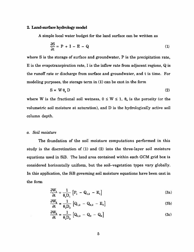
2. Land-mnTace hydrology model
A simple localwater budget for the land surface can be written as
_S--=P+I-E-Q (1)bt
where S is the storage of surface and groundwater, P is the precipitationrate,
E is the evapotranspiration rate,I isthe inflow rate from adjacent regions,Q is
the runoff rate or discharge from surface and groundwater, and t is time. For
modeling purposes, the storage term in (1)can be cast in the form
S = W 0, D (2)
where W is the fractional soil wetness, 0 < W < 1, e, is the porosity (or the
volumetric soil moisture at saturation), and D is the hydrologically active soil
column depth.
a. Soil moisture
The foundation of the soil moisture computations performed in this
study is the discretization of (1) and (2) into the three-layer soil moisture
equations used in SiB. The land area contained within each GCM grid box is
considered horizontally uniform, but the soil-vegetation types vary globally.
In this application, the SiB governing soil moisture equations have been cast in
the form
bWl- 1 [P1-Q1.2- E,] (3a)
bWs = __!_1 [Q1.2 - Q2.3 - Es] (3b)_t 0,D 2
_}W3 = 1 [q2.s - Q3 - Qb] (3c)bt e,D 3
5
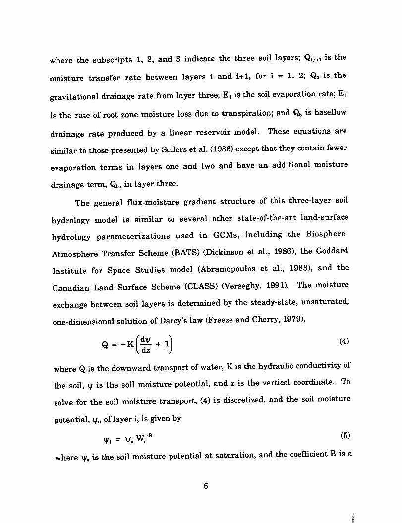
where the subscripts 1, 2, and 3 indicate the three soil layers; Qi,i.l is the
moisture transfer rate between layers i and i+l, for i = 1, 2; Q3 is the
gravitational drainage rate from layer three; E1 is the soil evaporation rate; E2
is the rate of root zone moisture loss due to transpiration; and Qb is baseflow
drainage rate produced by a linear reservoir model. These equations are
similar to those presented by Sellers et al. (1986) except that they contain fewer
evaporation terms in layers one and two and have an additional moisture
drainage term, Qb, in layer three.
The general flux-moisture gradient structure of this three-layer soil
hydrology model is similar to several other state-of-the-art land-surface
hydrology parameterizations used in GCMs, including the Biosphere-
Atmosphere Transfer Scheme (BATS) (Dickinson et al., 1986), the Goddard
Institute for Space Studies model (Abramopoulos et al., 1988), and the
Canadian Land Surface Scheme (CLASS) (Verseghy, 1991). The moisture
exchange between soil layers is determined by the steady-state, unsaturated,
one-dimensional solution of Darcy's law (Freeze and Cherry, 1979),
where Q is the downward transport of water, K is the hydraulic conductivity of
the soil, x? is the soil moisture potential, and z is the vertical coordinate. To
solve for the soil moisture transport, (4) is discretized, and the soil moisture
potential, _i, of layer i, is given by
_/_ = _/. Wi-B (5)
where W, is the soft moisture potential at saturation, and the coefficient B is a
6
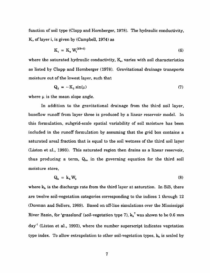
function of soil type (Clapp and Hornberger, 1978).
I_, of layer i, is given by (Campbell, 1974) as
K i = K 8 Wi (2B+3)
The hydraulic conductivity,
(6)
where the saturated hydraulic conductivity, I_, varies with soil characteristics
as listed by Clapp and Hornberger (1978). Gravitational drainage transports
moisture out of the lowest layer, such that
Q3 = - K3 sin(_) (7)
where 1_ is the mean slope angle.
In addition to the gravitational drainage from the third soil layer,
baseflow runoff from layer three is produced by a linear reservoir model. In
this formulation, subgrid-scale spatial variability of soil moisture has been
included in the runoff formulation by assuming that the grid box contains a
saturated areal fraction that is equal to the soil wetness of the third soil layer
(Liston et al., 1993). This saturated region then drains as a linear reservoir,
Qb, in the governing equation for the third soilthus producing a term,
moisture store,
Qb = kbW_ (8)
where kb is the discharge rate from the third layer at saturation. In SiB, there
are twelve soil-vegetation categories corresponding to the indices 1 through 12
(Dorman and Sellers, 1989). Based on off-line simulations over the Mississippi
River Basin, for 'grassland' (soil-vegetation type 7), kb 7 was shown to be 0.6 mm
day 1 (Liston et al., 1993), where the number superscript indicates vegetation
type index. To allow extrapolation to other soil-vegetation types, kb is scaled by
7
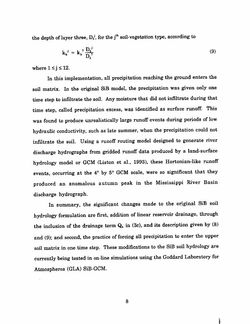
the depth of layer three, D3_, for the jth soil-vegetation type, according to
kb j -- kb 7 D3J (9)D3 7
where 1 < j < 12.
In this implementation, all precipitation reaching the ground enters the
soil matrix. In the original SiB model, the precipitation was given only one
time step to infiltrate the soil. Any moisture that did not infiltrate during that
time step, called precipitation excess, was identified as surface runoff. This
was found to produce unrealistically large runoff events during periods of low
hydraulic conductivity, such as late summer, when the precipitation could not
infiltrate the soil. Using a runoff routing model designed to generate river
discharge hydrographs from gridded runoff data produced by a land-surface
hydrology model or GCM (Liston et al., 1993), these Hortonian-like runoff
events, occurring at the 4 ° by 5 ° GCM scale, were so significant that they
produced an anomalous autumn peak in the Mississippi River Basin
discharge hydrograph.
In summary, the significant changes made to the original SiB soil
hydrology formulation are first, addition of linear reservoir drainage, through
the inclusion of the drainage term Qb in (3c), and its description given by (8)
and (9); and second, the practice of forcing all precipitation to enter the upper
soil matrix in one time step. These modifications to the SiB soil hydrology are
currently being tested in on-line simulations using the Goddard Laboratory for
Atmospheres (GLA) SiB-GCM.
8

bo Evapotranspiration
Soil moisture dependent evapotranspiration is computed by scaling the
potential evapotranspiration, Ep, by a factor _i,
Ei = _i Ep (10)
where the subscript i = 1, 2 identifies the soil layer of interest, and E is the
actual evaporation rate. For the case of vegetated land, 92 is defined to be the
soil water stress factor for the second soil layer, f(_2), given by Xue et al. (1991),
f(_¢2) = 1- exp(-c 2 (c 1 - ln(-xV2)) ) 0<f(_)<l (11)
where c, and c2 are empirical constants representing the progression of
closing stomata. Values of c, and c2 for the different vegetation types are given
in Table 1, where the swapping of cl and cs in the table presented by Xue et al.
(1991) has been corrected. For the case of soil-vegetation type 11 (bare soil), _, -
W,, the soil wetness of the uppermost soil layer.
c. Atmospheric forcing
In its reduced form described above, the SiB land-surface hydrology
parameterization was forced using daily values of potential evaporation and
surface station precipitation climatology. Potential evapotranspiration, Ep,
was computed following Thornthwaite (1948), which requires a surface air
temperature representative of potential conditions. To account for measured
surface air temperatures, that may not have been collected under conditions of
zero soil moisture stress, we let the ratio of actual transpiration to potential
transpiration be a function of normalized difference vegetation index (NDVI),
9
available from satellite measurements. This has eliminated the need to
consider root zone soil moisture and the soil water storage capacity when
computing the temperature correction, and has also prevented errors in
measured precipitation from affecting the computations (Mintz and Walker,
1993).
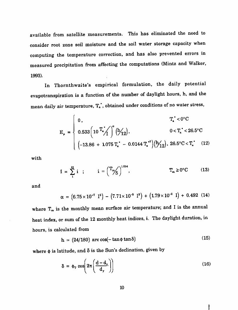
In Thornthwaite's empirical formulation, the daily potential
evapotranspiration is a function of the number of daylight hours, h, and the
mean daily air temperature, T.', obtained under conditions of no water stress,
Ep --
with
0, Ta* < 0°C
/ °0.533 10 (_2)' 0 < T.*< 26.5°C
(12)
12 (T /,_1.514
I = Ei ; i = _ Y5) ' Tm>0°c (13)1
and
a = (6.75×10 -_ 13) -(7. 71x10-5 I2) + (1"79x10-2 I)+ 0.492 (14)
where Tm is the monthly mean surface air temperature; and I is the annual
heat index, or sum of the 12 monthly heat indices, i. The daylight duration, in
hours, is calculated from
h = (24/180) arc cos(- tan_ tanS) (15)
where _ is latitude, and 5 is the Sun's declination, given by
(16)
10
where _ is the latitude of the Tropic of Cancer (23.45°), d is the Gregorian Day,
dr is the day of the summer solstice (173), and dy is the average number of days
in a year (365.25). Poleward of 50 ° latitude, Thornthwaite defined h to be the
same as h at 50 °.
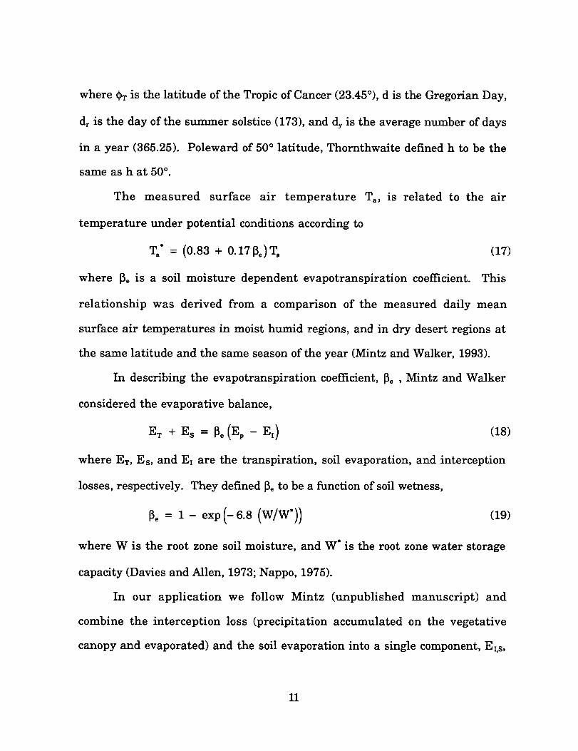
The measured surface air temperature Ta, is related to the air
temperature under potential conditions according to
T,* = (0.83 + 0.17_,)T, (17)
where [3e is a soil moisture dependent evapotranspiration coefficient. This
relationship was derived from a comparison of the measured daily mean
surface air temperatures in moist humid regions, and in dry desert regions at
the same latitude and the same season of the year (Mintz and Walker, 1993).
In describing the evapotranspiration coefficient, [3e , Mintz and Walker
considered the evaporative balance,
where ET, Es, and E_ are the transpiration, soil evaporation, and interception
losses, respectively. They defined [3e to be a function of soil wetness,
_e : 1- exp(-6.8 (W/W*)) (19)
where W is the root zone soil moisture, and W* is the root zone water storage
capacity (Davies and Allen, 1973; Nappo, 1975).
In our application we follow Mintz (unpublished manuscript) and
combine the interception loss (precipitation accumulated on the vegetative
canopy and evaporated) and the soil evaporation into a single component, E_,s,
11
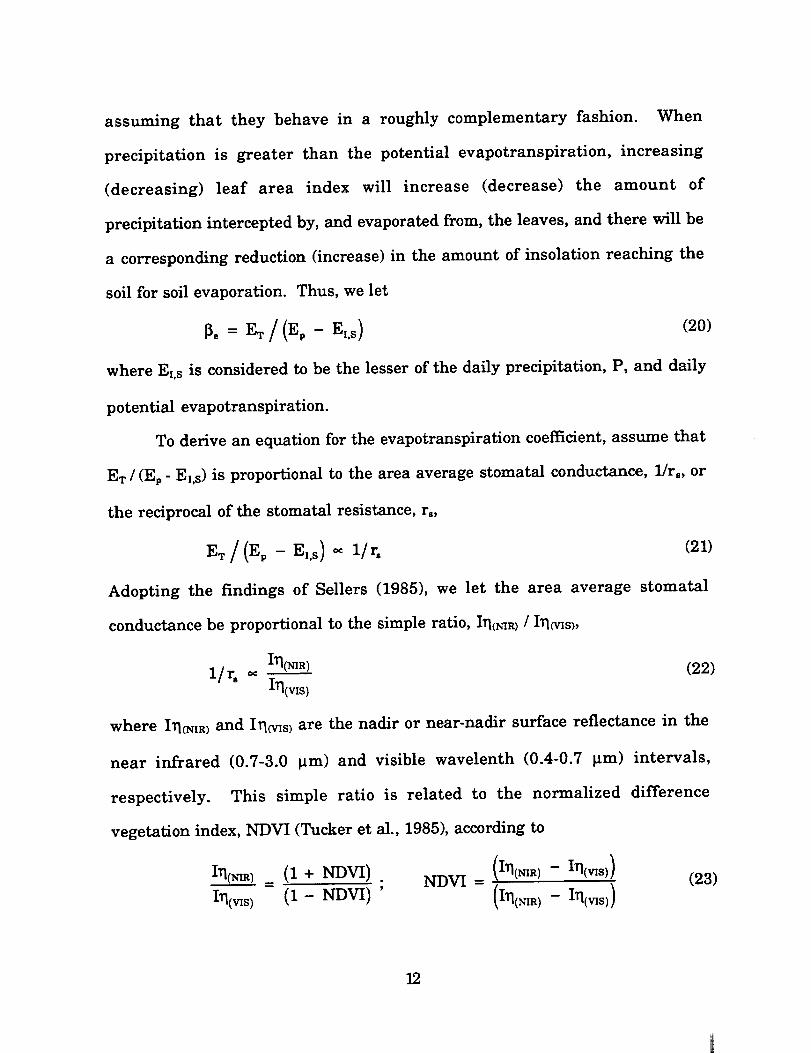
assuming that they behave in a roughly complementary fashion. When
precipitation is greater than the potential evapotranspiration, increasing
(decreasing) leaf area index will increase (decrease) the amount of
precipitation intercepted by, and evaporated from, the leaves, and there will be
a corresponding reduction (increase) in the amount of insolation reaching the
soil for soil evaporation. Thus, we let
where E_.s is considered to be the lesser of the daily precipitation, P, and daily
potential evapotranspiration.
To derive an equation for the evapotranspiration coefficient, assume that
ET / (Ep - E_.s) is proportional to the area average stomatal conductance, l/r,, or
the reciprocal of the stomatal resistance, rs,
E T /(Ep - E,.s) _ l/rs (21)
Adopting the findings of Sellers (1985), we let the area average stomatal
conductance be proportional to the simple ratio, ITkmR_ / ITl_s_,
Iq(_nR) (22)
1/r, o, ITl(VlS)
where I_l(mm and I_ns) are the nadir or near-nadir surface reflectance in the
near infrared (0.7-3.0 _tm) and visible wavelenth (0.4-0.7 _tm) intervals,
respectively. This simple ratio is related to the normalized difference
vegetation index, NDVI (Tucker et al., 1985), according to
ITI(NIR).= (1 + NDVI) . NDVI = (BI(Nm)- Iq(v,s)) (23)
ITI0ns ) (1 - NDVI) ' (ITl(ma) - ITI0ns))
12
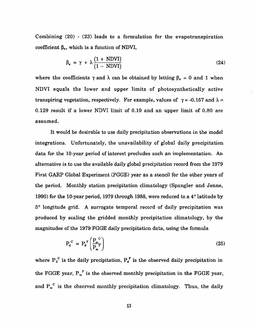
Combining (20) - (23) leads to a formulation for the evapotranspiration
coefficient _e, which is a function of NDVI,
9, = 7 + X(I+ NDVI)(1 - NDVI) (24)
where the coefficients 7 and k can be obtained by letting _ = 0 and 1 when
NDVI equals the lower and upper limits of photosynthetically active
transpiring vegetation, respectively. For example, values of 7 = -0.157 and _. =
0.129 result if a lower NDVI limit of 0.10 and an upper limit of 0.80 are
assumed.
It would be desirable to use daily precipitation observations in the model
integrations. Unfortunately, the unavailability of global daily precipitation
data for the 10-year period of interest precludes such an implementation. An
alternative is to use the available daily global precipitation record from the 1979
First GARP Global Experiment (FGGE) year as a stencil for the other years of
the period. Monthly station precipitation climatology (Spangler and Jenne,
1990) for the 10-year period, 1979 through 1988, were reduced to a 4 ° latitude by
5 ° longitude grid. A surrogate temporal record of daily precipitation was
produced by scaling the gridded monthly precipitation climatology, by the
magnitudes of the 1979 FGGE daily precipitation data, using the formula
(25)
where Pa c is the daily precipitation, Pa F is the observed daily precipitation in
the FGGE year, PZ is the observed monthly precipitation in the FGGE year,
and pC is the observed monthly precipitation climatology. Thus, the daily
13
precipitation forcing preserves measured monthly magnitudes and occurs at
the frequency of the observed 1979 precipitation events. Admittedly, in the
natural system, the frequency of precipitation events will vary from one year to
the next. In this application, we have assumed that when the daily computed
soil moisture, evapotranspiration, and runoff are compiled to produce monthly
means, the resulting values will be representative of the period in question.
The availability of daily precipitation data over the United States is currently
being used to test this assumption. In the integrations, all precipitation data
were treated as rainfall. Station monthly mean surface air temperature data
were gridded and linearly interpolated to provide mean daily air temperatures.
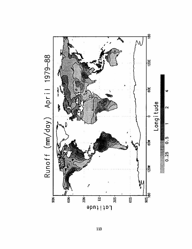
3_ Presentation of data
By aggregating the daily data produced by the model integrations, global
monthly mean precipitation, evapotranspiration, runoff, and soil moisture for
each of SiB's three soillayers have been produced for each month of the 10-year
period, 1979 through 1988. In this technical memorandum, global distribution
maps illustrating 10-year (1979 - 1988) monthly averages of the monthly mean
precipitation, evapotranspiration, root zone soil moisture, and runoff fields
have been plotted. In addition, the standard deviations of the monthly mean
precipitation, evapotranspiration, root zone soilmoisture, and runoff for the 10-
year period are also included. These are found in the section titled:
"HYDROLOGIC FIELDS: 10-Year Average of Monthly Means, and Standard
Deviations" under the subheadings, PRECIPITATION (January - December),
EVAPOTRANSPIRATION (January - December), ROOT ZONE SOIL
14
WETNESS (January - December), and RUNOFF (January - December).
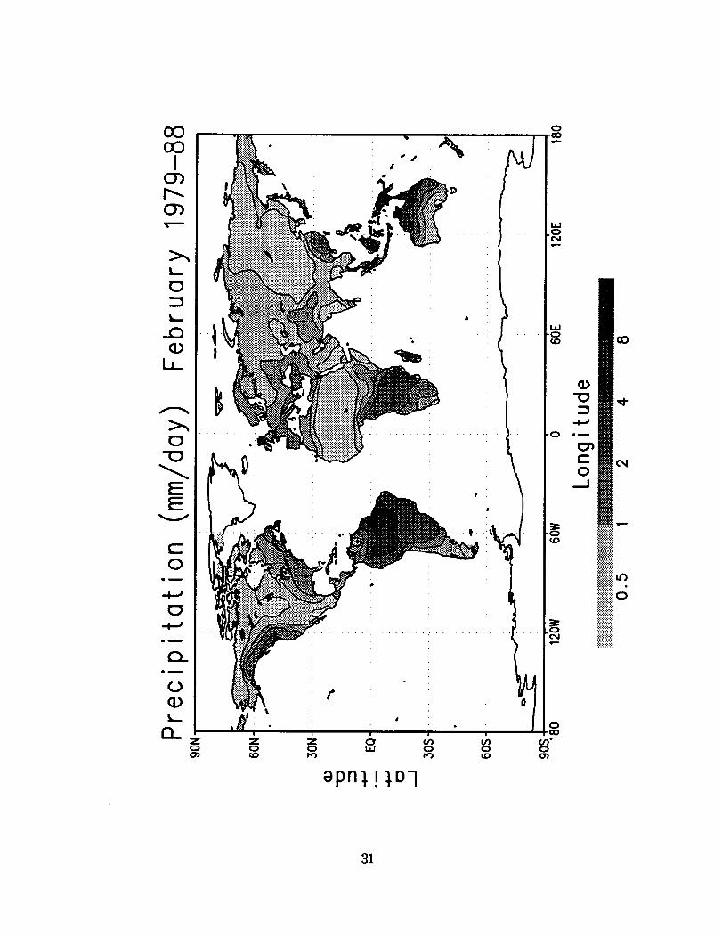
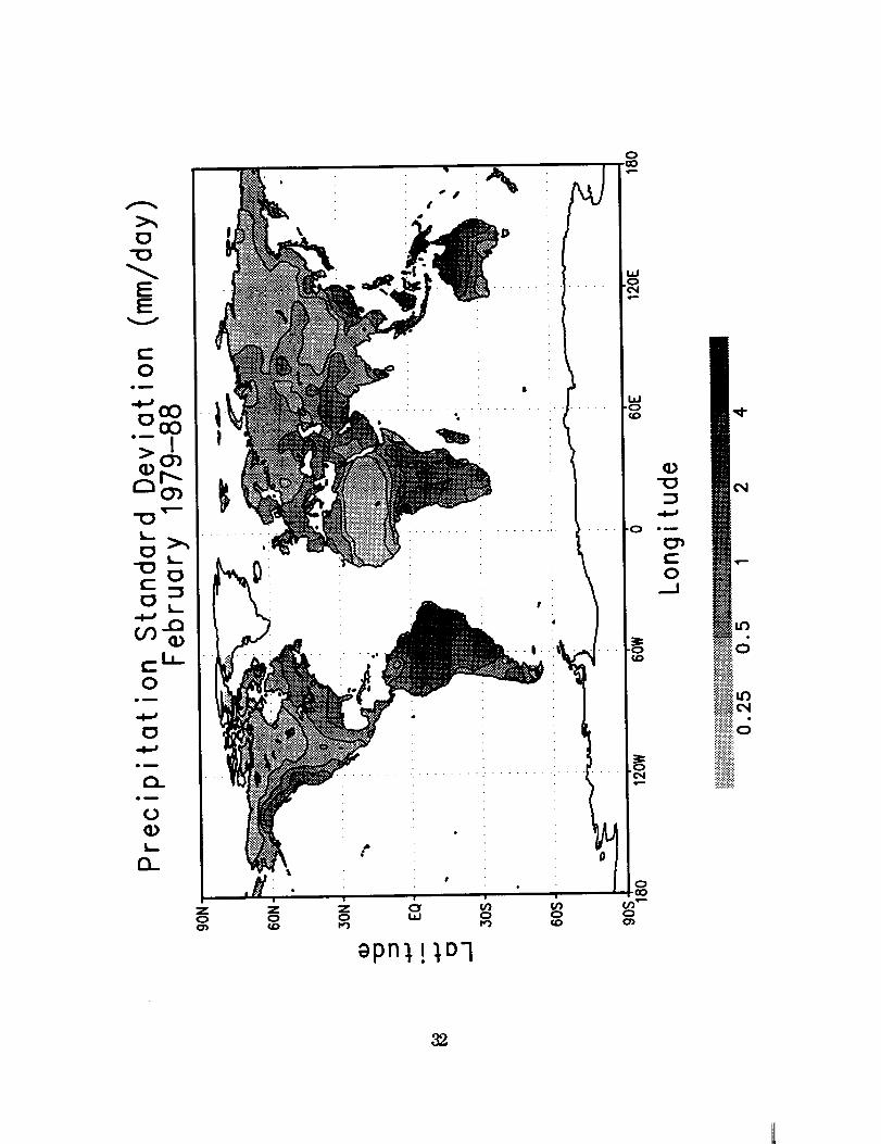
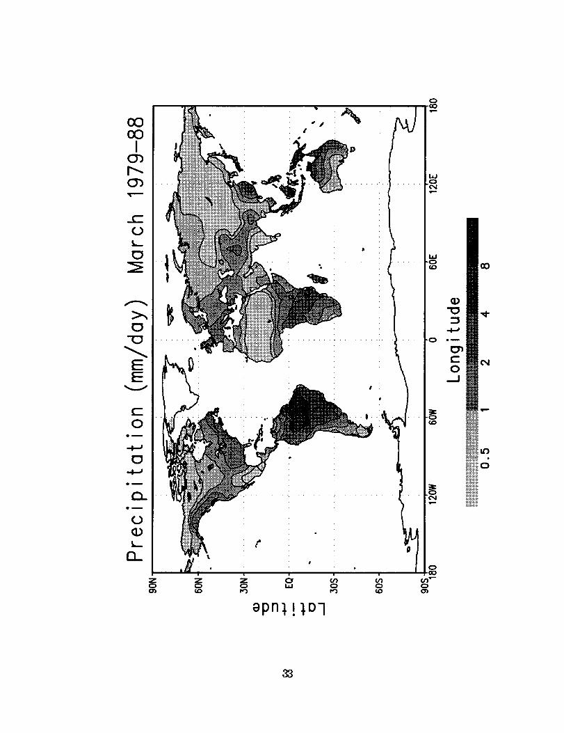
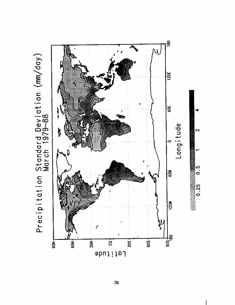
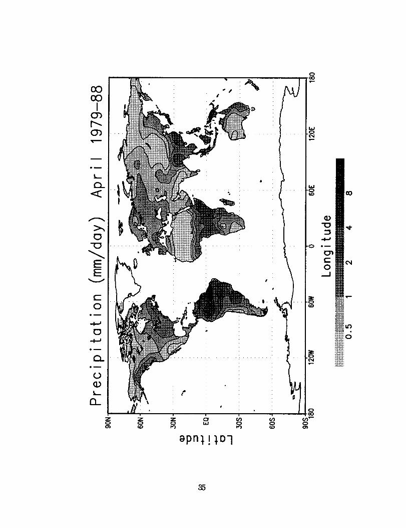
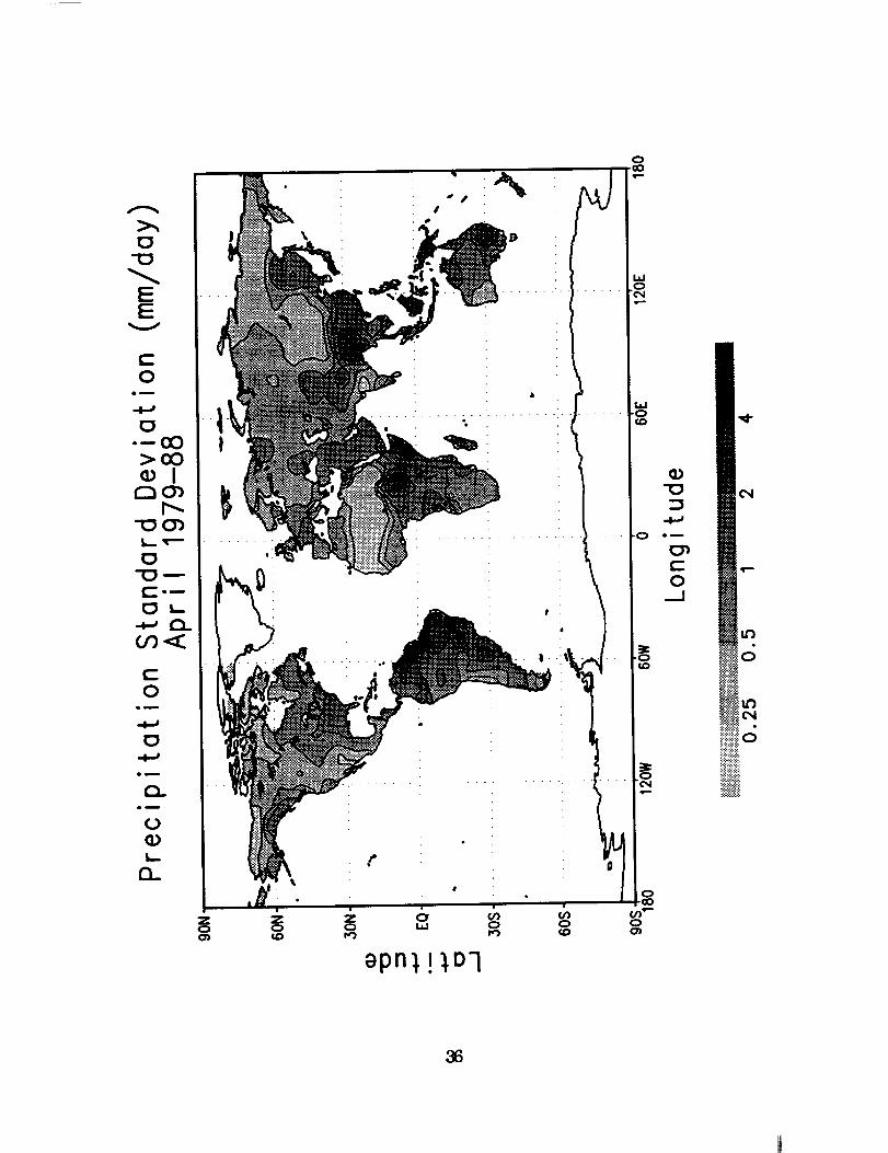
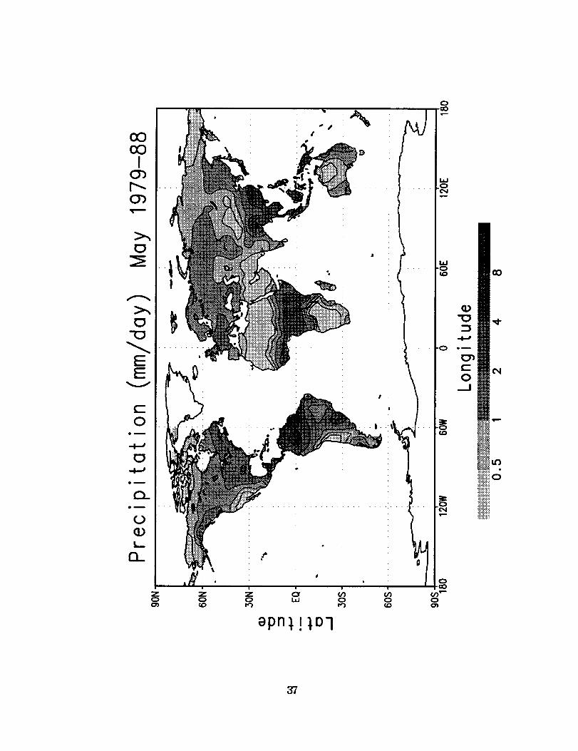
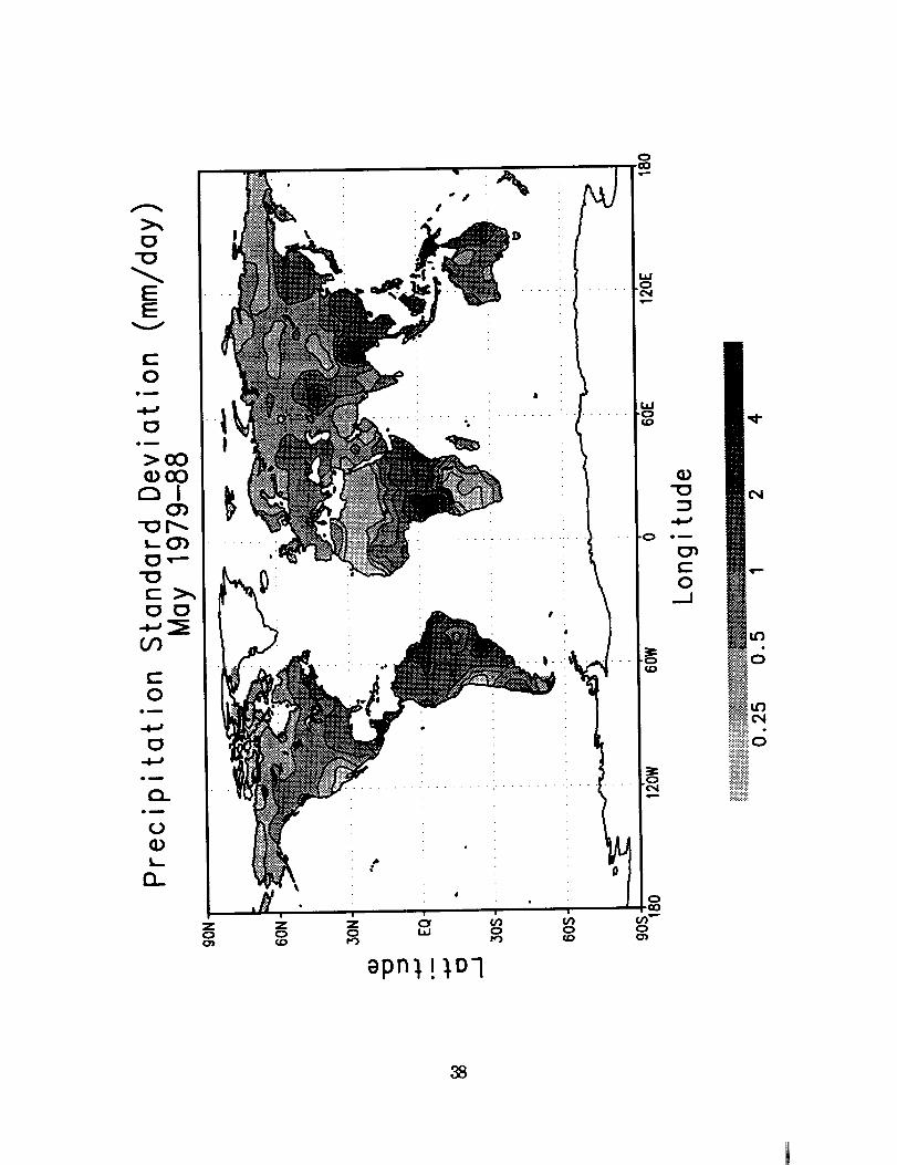
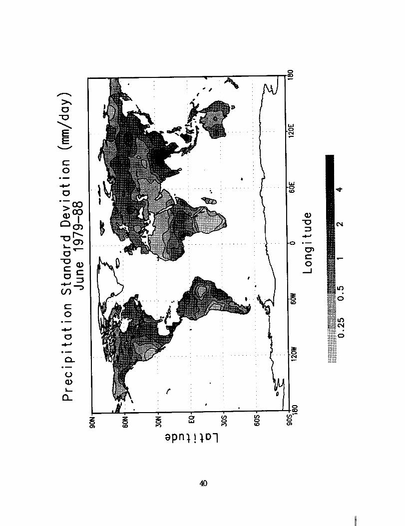
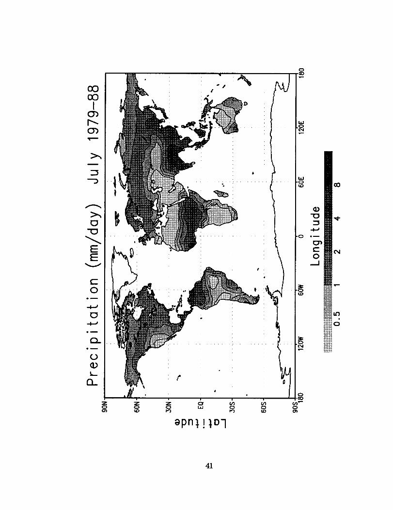
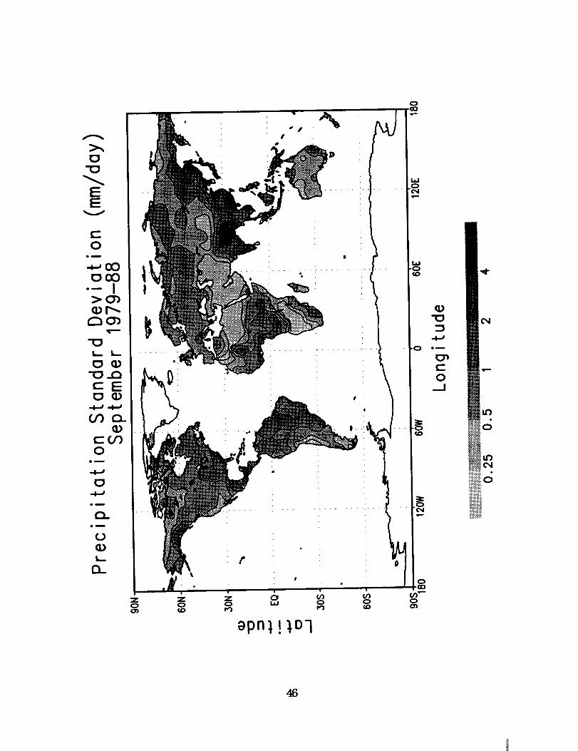
Referring to the precipitation figures, in January, maximum
precipitation values of over 8 mm day 1 occur in the tropical regions south of
the equator in South America, Africa, the Pacific Islands, and Australia. In
addition, a January precipitation maximum is found in the mountainous
regions surrounding the Gulf of Alaska. In January, regions of precipitation
less than 0.5 mm day "1 include Arctic North America, the central United
States, central Africa, and central Asia. By July, the tropical precipitation
peak has shifted north of the equator to include South and Central America,
Africa, and India. The precipitation minimum in central Africa has shifted
north. A minimum of less than 0.5 mm day 1 in July also exists in southern
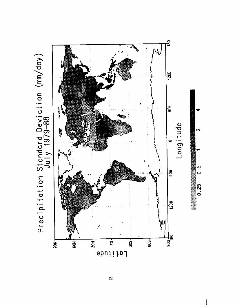
Africa, central South America, and central Australia. In general, the
precipitation standard deviation patterns correspond to the precipitation
patterns, with the highest standard deviations occurring in the regions of
highest precipitation.
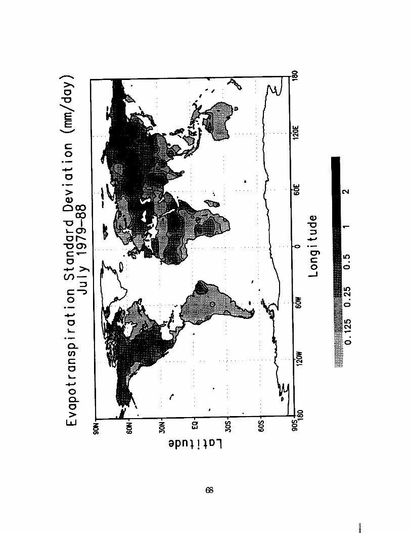
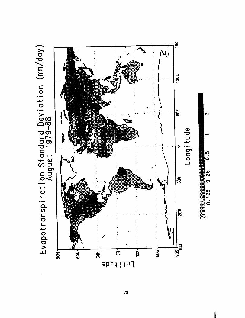
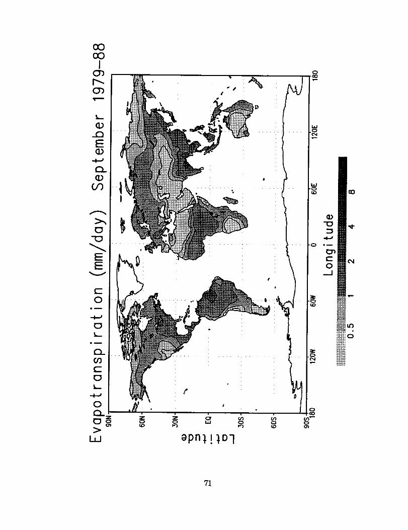
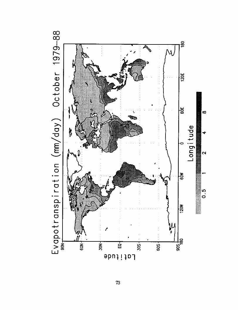
Evapotranspiration is minimal, less than 0.5 mm day 1, in the Northern
Hemisphere in January, while south of the equator, evapotranspiration is
typically greater than 2 mm day _. In May, regions north of 30 ° N latitude
show a significant increase in evapotranspiration. By July, Northern
Hemisphere evapotranspiration has increased sharply, typically being
between 2 and 4 mm day 1, with the exception of the regions of northern Africa
and Arabia, where values less than 0.5 mm day "1 are typical. In general, the
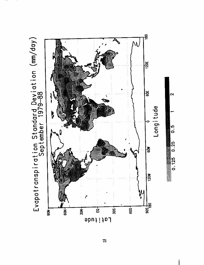
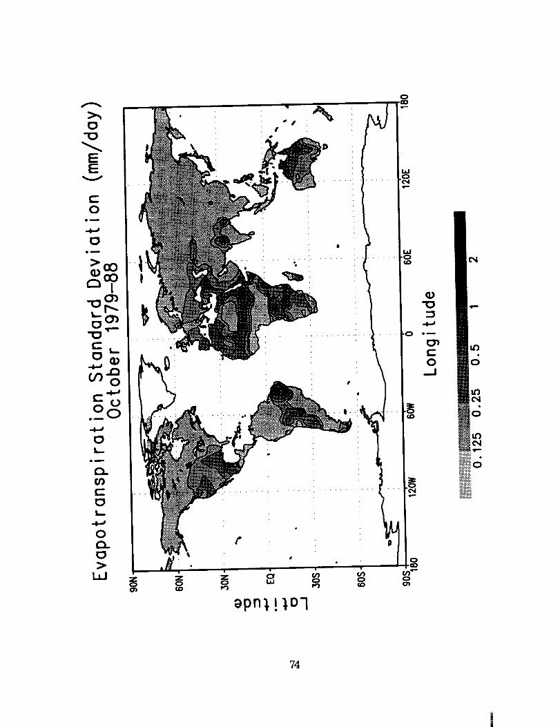
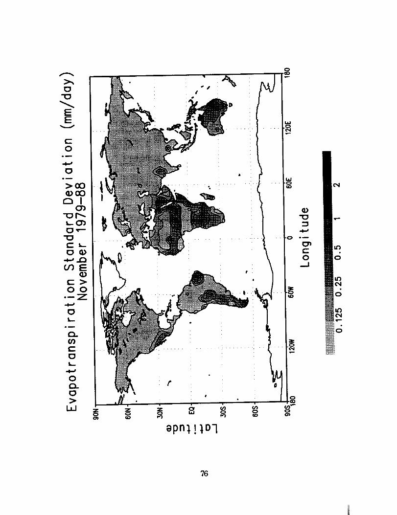
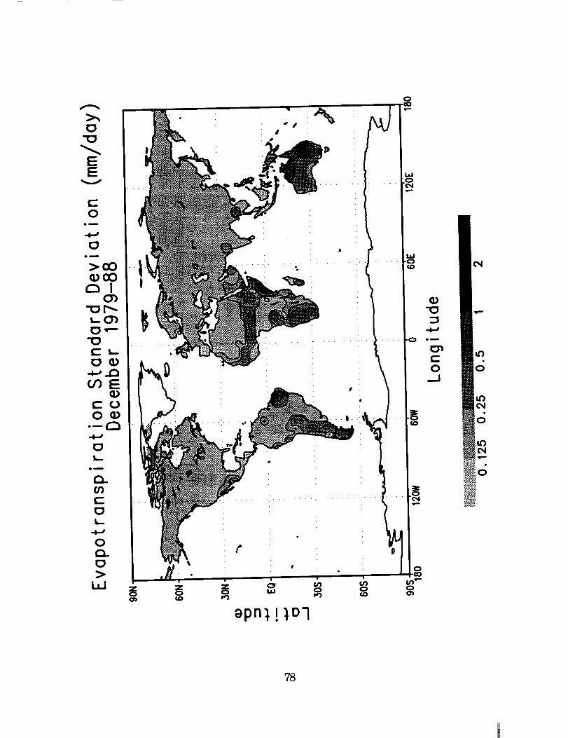
evapotranspiration standard deviation patterns correspond to the
15
evapotranspiration patterns, with the highest standard deviations occurring
in the regions of highest evapotranspiration. Typically the evapotranspiration
standard deviation displays more structure than the relatively smooth
evapotranspiration patterns. In the Southern Hemisphere winter, South
America has minimal evapotranspiration standard deviation.
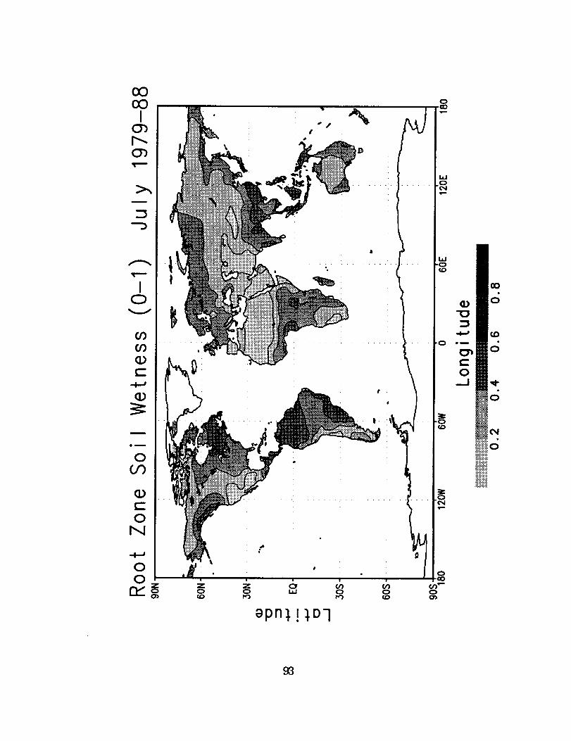
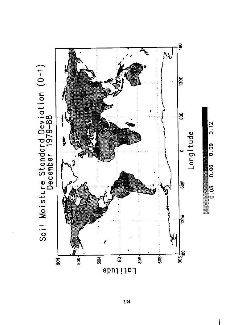
Referring to the soil wetness figures, the lowest January root zone soil
wetness values are found in the southwest United States, Mexico, southern
South America and Africa, the Sahara, Arabia, and central Asia. These
minimum soil moisture fractions are typically between 0.15 and 0.2.
Maximum values, between 0.6 and 0.8, are found in the tropics, in the middle
latitude storm belt regions such as the northwest coastal regions of the United
States and Canada, and in Europe. In July, subtle changes in the soil
moisture patterns are evident over the globe, but nothing as dramatic as the
differences found in the precipitation and evapotranspiration patterns. In
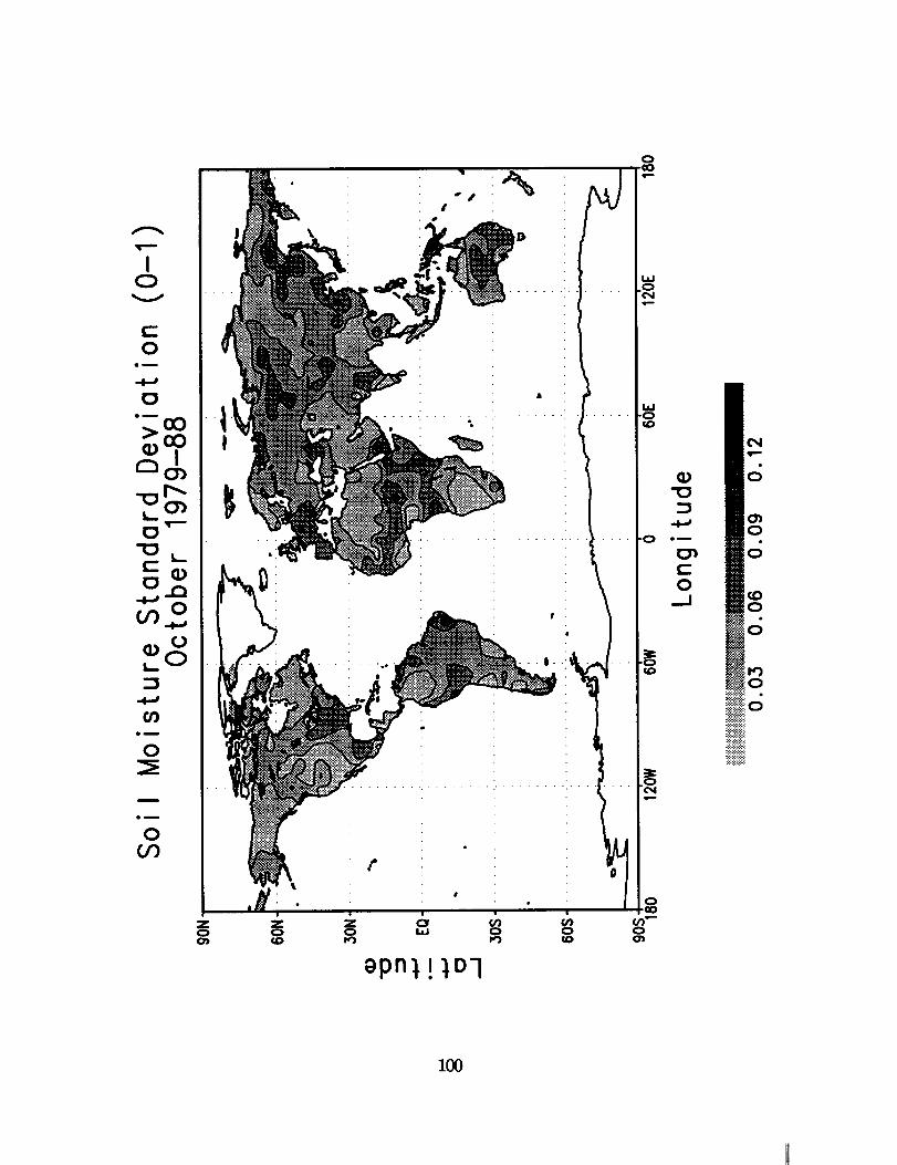
general, the soil wetness standard deviations vary considerably. Note that in
the SiB evapotranspiration formulation, although it does depend on soil-
vegetation type, evapotranspiration occurs at the potential rate for soil wetness
values around 0.60 and evapotranspiration becomes zero at a soil wetness
value of near 0.30. As a consequence, a 0.10 change in soil wetness is able to
have a significant influence on evapotranspiration. Typically the soil wetness
standard deviations are greatest in the tropics and decrease with increasing
latitude.
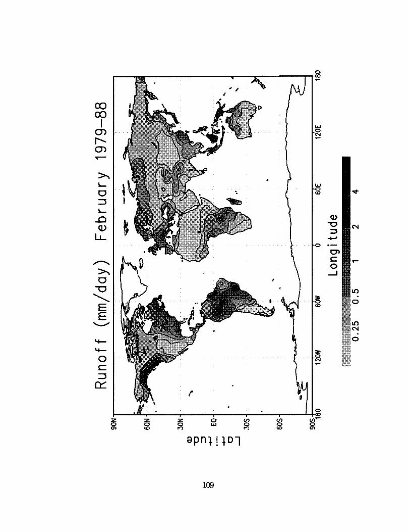
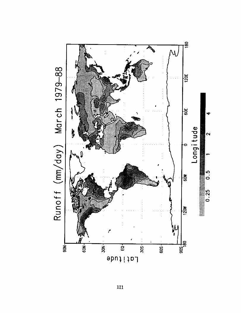
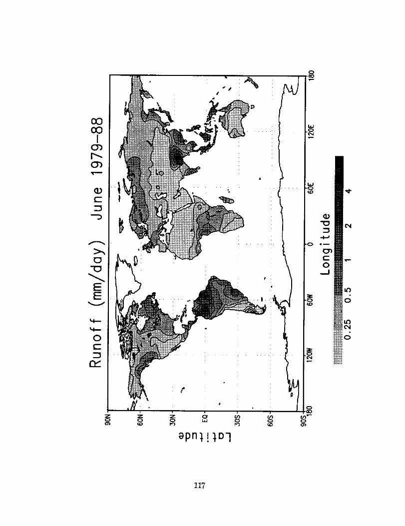
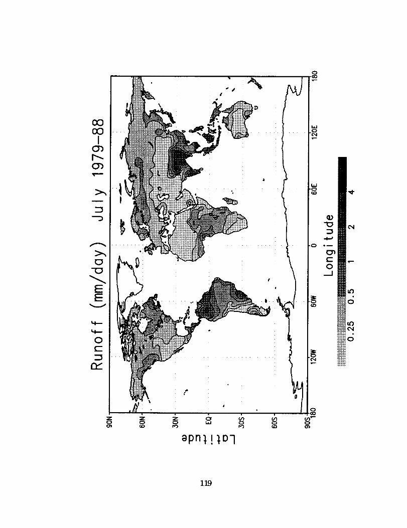
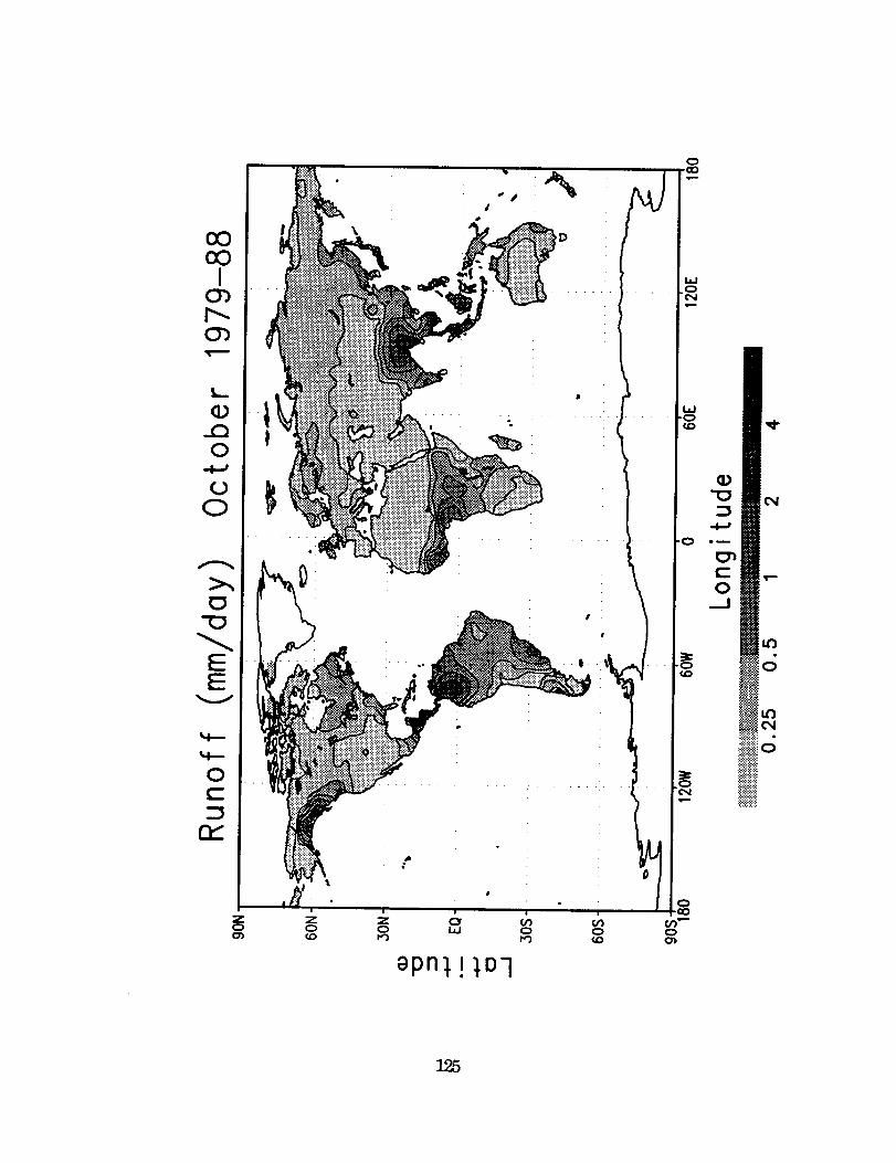
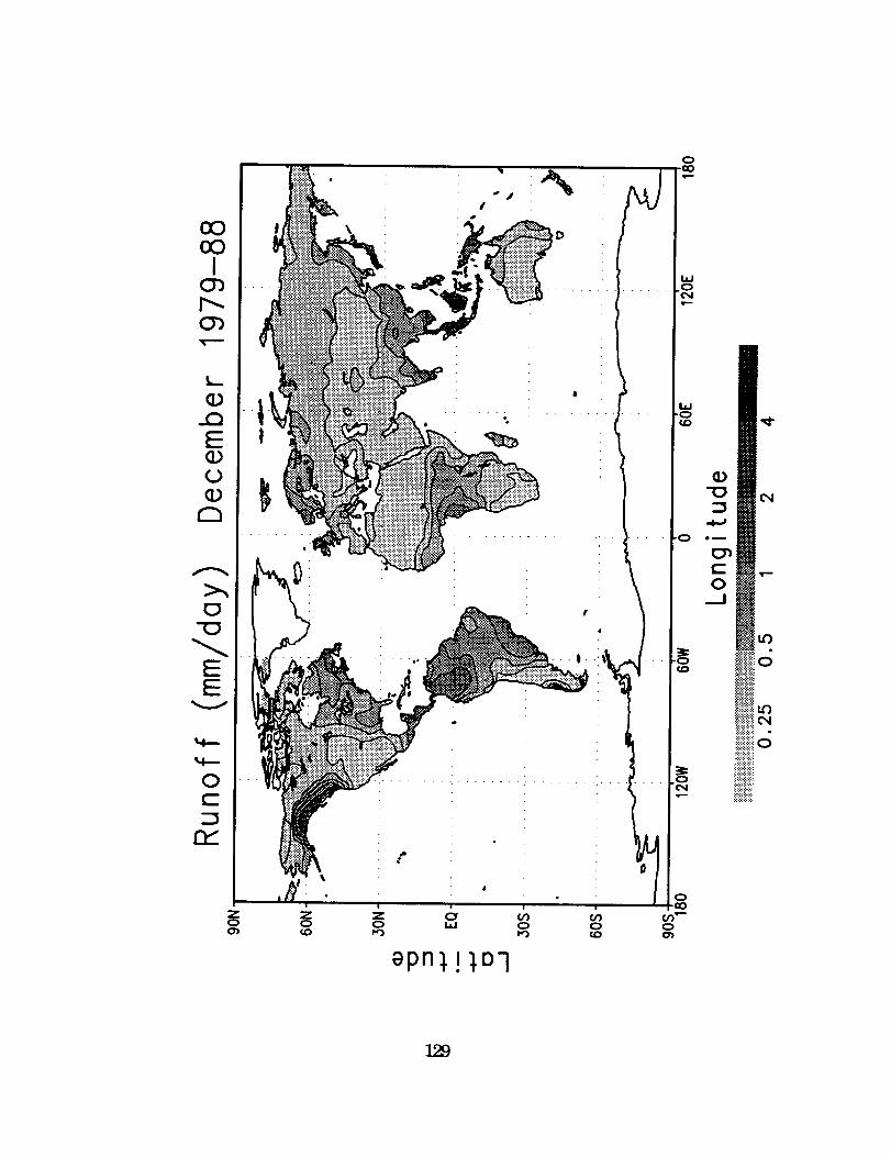
Peak January runoff occurs in the region surrounding the Gulf of
Alaska and in the tropics of South America, Africa, the Pacific Islands, and
16
central Australia. In July, the tropical runoff maximum has shifted north,
and India and regions to the north and east are producing runoff values
greater than 8 mm day "1. Since runoff is strongly a function of soil moisture,
the relatively subtle seasonal changes in soil moisture are reflected in the
subtle seasonal changes in runoff. The one significant exception to this is the
dramatic seasonal change in runoff produced by the increased precipitation
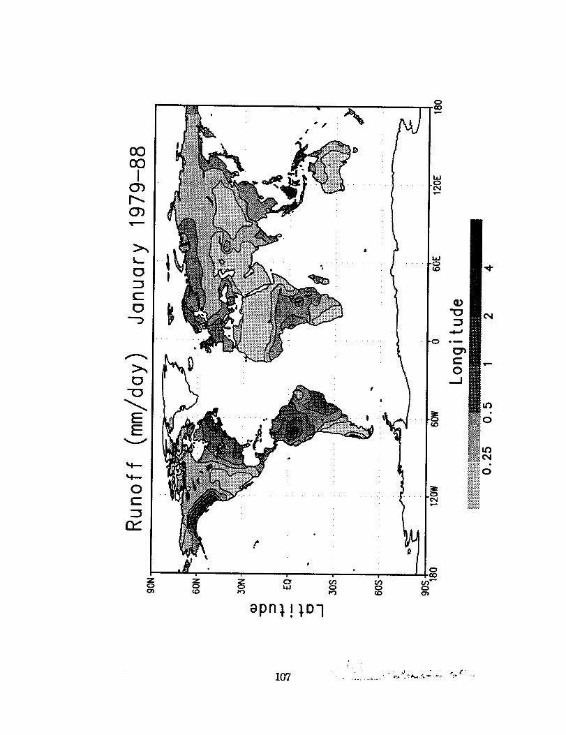
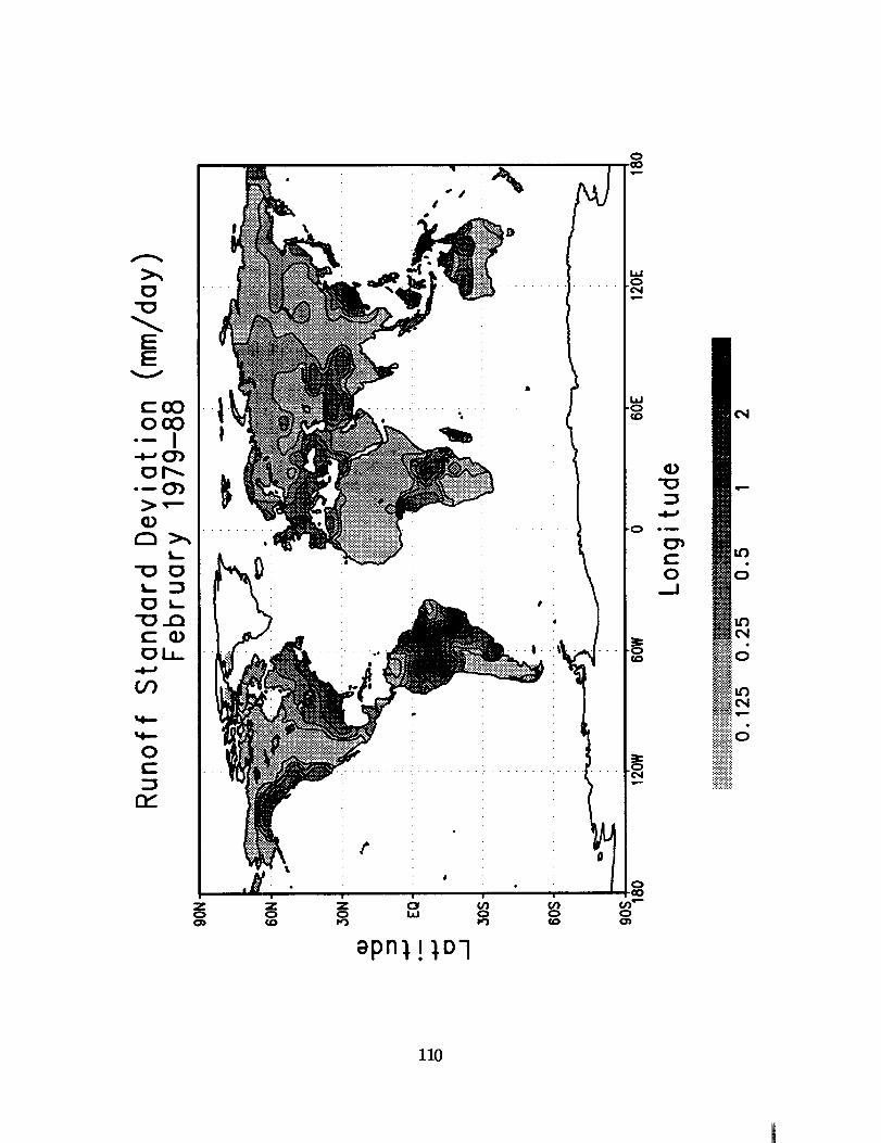
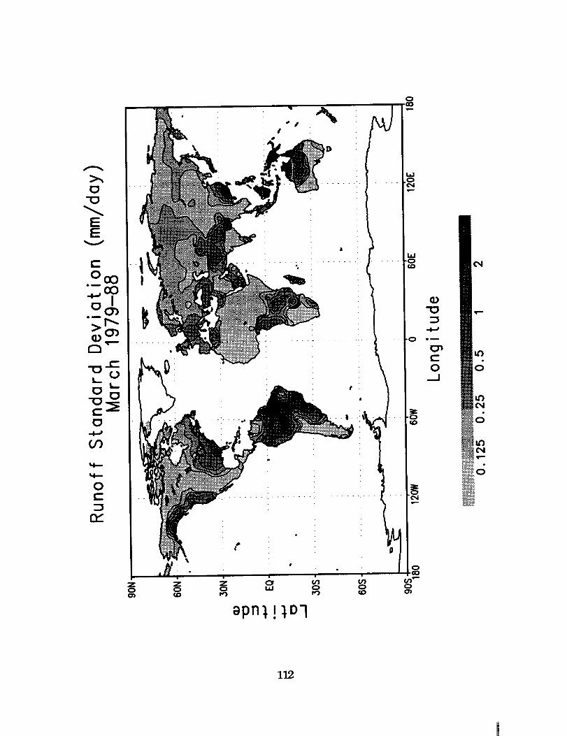
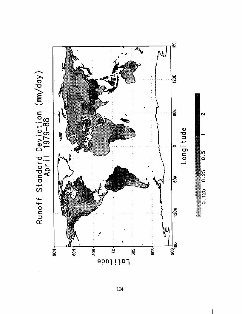
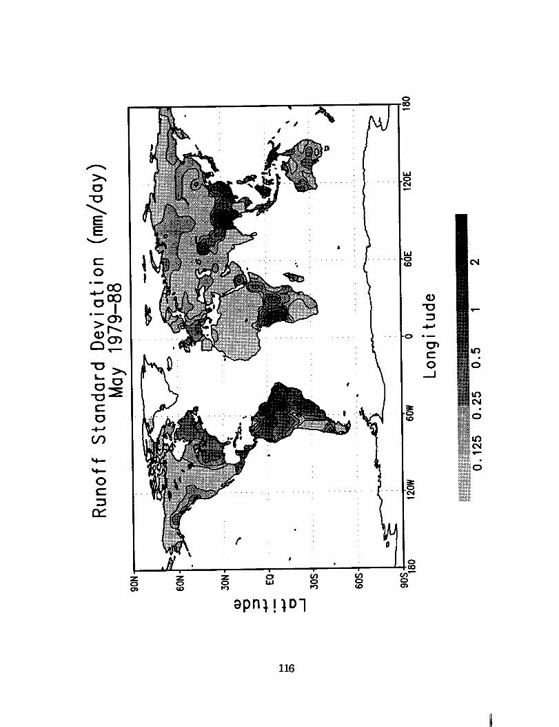
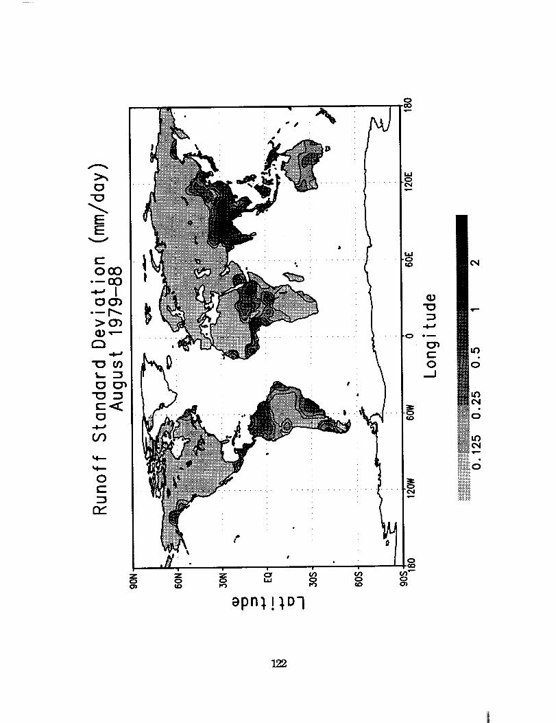
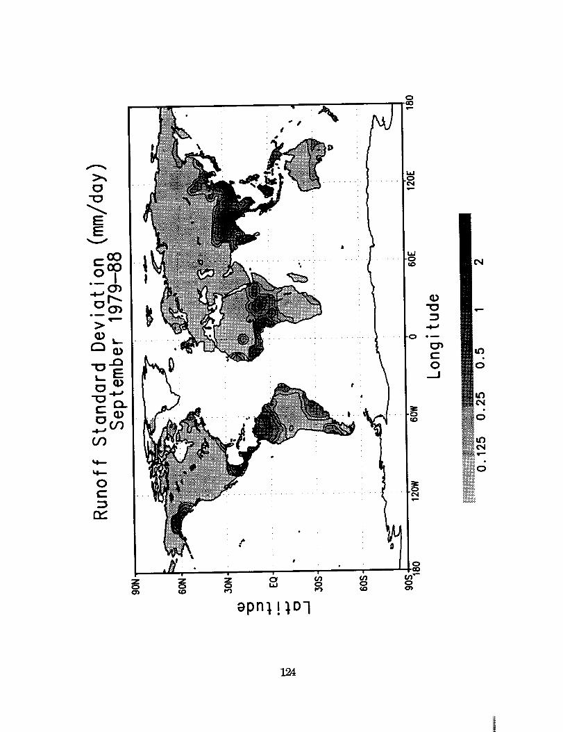
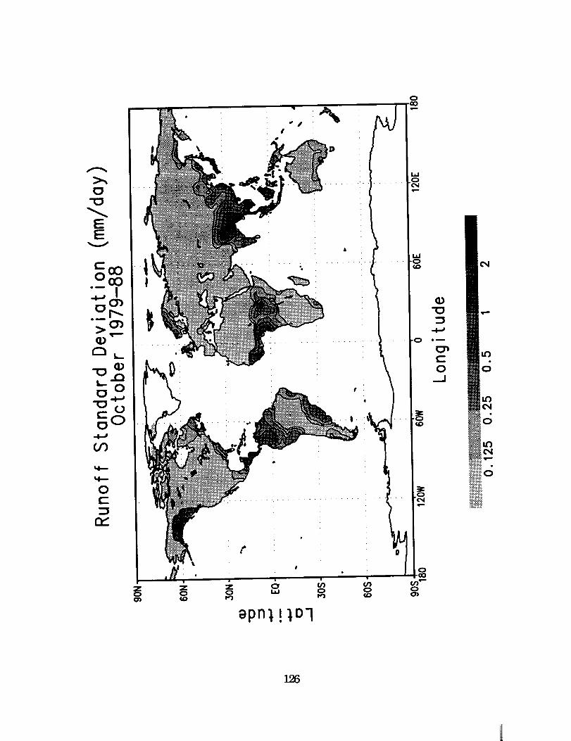
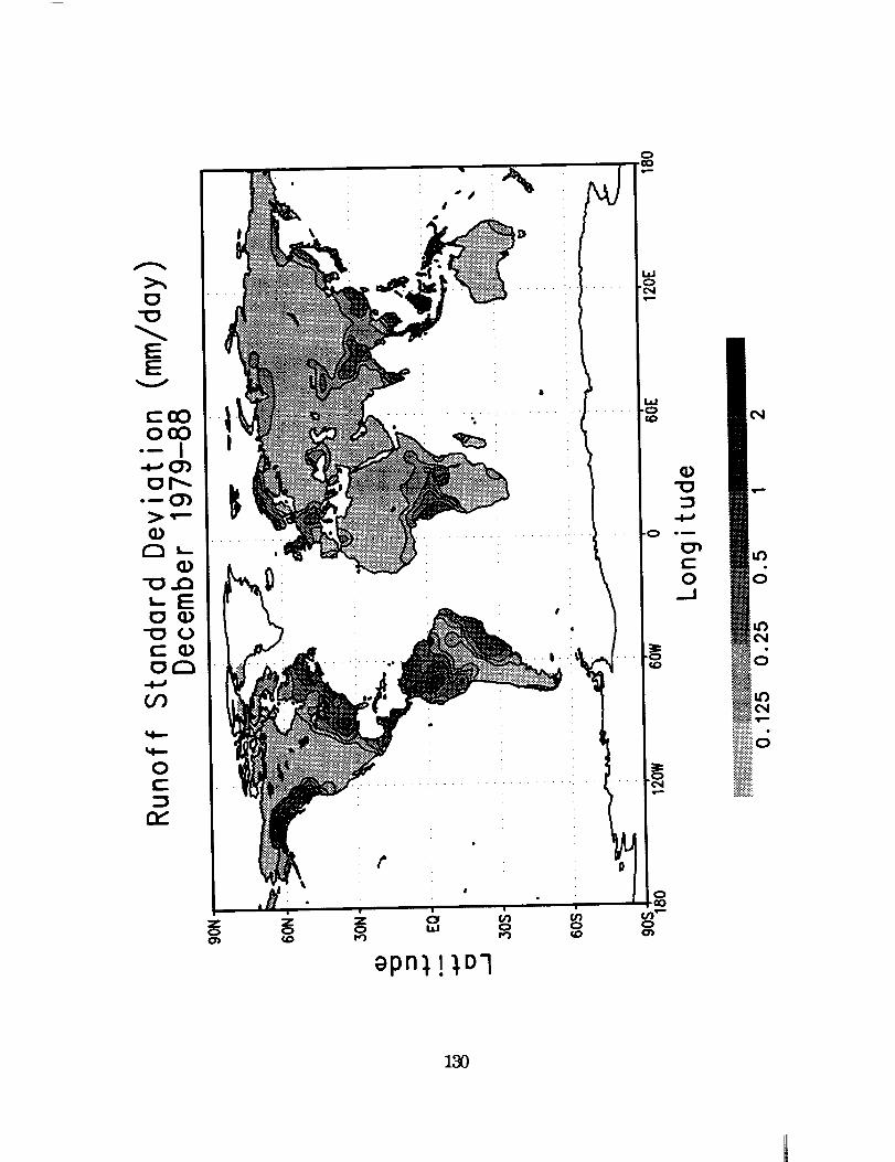
during the Indian monsoon. In general, the runoff standard deviation
patterns correspond to the runoff patterns, with the highest standard
deviations occurring in the regions of highest runoff. Compared to the
minimal runoff standard deviations occurring in the Northern Hemisphere
during the Northern Hemisphere summer, the tropics contain relatively high
standard deviations during this period.
As part of the model integrations, global monthly mean soil moisture for
each of SiB's three soil layers were produced for each month of the 10-year
period. These soil moisture fields are currently being used as soil moisture
initial conditions during climate simulations using the version of the GLA
GCM that employs the SiB land-surface parameterization.
4. Concluding snmmary
An analysis scheme to generate global evapotranspiration and soil
moisture fields, using key components of the Simple Biosphere Model, has
been developed. Two modifications have been made to the original SiB soil
hydrology formulation: a linear reservoir drainage term has been added to the
third soil layer, and all precipitation is forced to enter the upper soil matrix
17

during each time step. The influence of these modifications is being tested in
the Goddard Laboratory for Atmospheres SiB-GCM. In addition, the analysis
scheme incorporates a simplified computation of evapotranspiration based on
SiB evapotranspiration functions.
The method requires atmospheric forcing of precipitation and potential
evapotranspiration. Potential evapotranspiration is computed using the
method of Thornthwaite, where the observed air temperatures have been
adjusted to represent potential conditions by using normalized difference
vegetation index (NDVI) data determined from satellite observations. The
analysis was run for 10 years, 1979 through 1988. In performing the model
integrations, it would be desirable to use global observed daily precipitation. To
circumvent the unavailability of global daily precipitation data for the period
1979 through 1988, we use the daily global precipitation record from the 1979
FGGE year as a stencil for the other years of the period. Thus, by using
observed monthly mean precipitation data, we produce a 10-year, daily
precipitation record which preserves measured monthly magnitudes, and
occurs at the frequency of the observed 1979 FGGE year precipitation events.
The scheme represents an efficient methodology for generating soil
moisture initialization fields for GCMs; it can also be applied to other land-
surface hydrology parameterizations being used in GCMs, through a
substitution of the parameterizations' soil hydrology and evapotranspiration
functions. The resulting soil moisture fields are compatible with the
atmospheric forcing of observed precipitation and surface air temperature
climatology. In addition, these fields are computed in a manor consistent with
18

the soil hydrology and evapotranspiration representations found in the specific
GCM land-surface hydrology parameterization of interest.
Validation of data sets such as the ones described here is an important
and necessary step in the development and refinement of information used in
climate simulations using GCMs. At seasonal and continental scales,
terrestrial precipitation inputs are considered relatively well known, despite
the scarcity of data in some regions of the world. In addition, river discharge
measurements are readily available and are being used for model validation
over large areas (Liston et al., 1993). This river discharge is an important
integrator of the hydrologic cycle, and is able to provide much needed insight
into whether or not the models produce realistic terrestrial water balances.
Evapotranspiration comprises a significant fraction of the moisture transport
within the hydrologic cycle; unfortunately, direct validation of land-surface
evapotranspiration is difficult, and it is generally approximated using indirect
methods that utilize air temperature or radiation observations. Soil moisture
data from remote sensing measurements are now becoming available for
comparison with modeled fields. A useful feature of these observations is the
measurement of subgrid-scale soil moisture variability. These data and other
satellite-derived products are expected to assist in the formulation of next
generation runoff and evapotranspiration schemes, and thus provide a
valuable contribution to future land-surface modeling efforts. The resulting
improved understanding and description of terrestrial hydrology will add to
the quality of global climate simulations.
19
NUMERICAL DATA. Input and derived fields described in this
technical memorandum are available for all months of the 10-year period, 1979
through 1988, in the form of grid-area numerical values. They are available in
printed tables, on magnetic tape, and via Internet using standard file transfer
protocal (f_p). Contact the authors, Climate and Radiation Branch, Code 913,
Laboratory for Atmospheres, NASA/Goddard Space Flight Center, Greenbelt,
Maryland 20771.
ACKNOWLEDGEMENTS. Unpublished algorithms and empirical
relationships developed by Professor Y. Mintz have been invaluable in the
development of this method for estimating global soil moisture fields. We also
thank J. Schemm for providing the gridded precipitation data sets. Support for
this research was provided by the NASA Land and Climate program offices.
2O
REFERENCES
Abramopoulos, F.,C. Rosenzweig and B. Choudhury, 1988: Improved ground
hydrology calculations for global climate models (GCMs): Soil water
movement and evapotranspiration. J. Climate, 1, 921-941.
Budyko, M.I., 1956: Teplovoi Balans Zemnoi Poverkhnosti. Gidrometeoizdat,
Leningrad; Heat Balance of the Earth's Surface, translated by N.A.
Sepanova, U.S. Weather Bur., Washington, D.C., 1958. MGA 8.5-20, 13E-
286, IIB-25,259 pp.
Campbell, G.S., 1974: A simple method for determining unsaturated
conductivity from moisture retention data. Soil Sci., 117, 311-314.
Clapp, R.B., and G.M. Hornberger, 1978: Empirical equations for some soil
hydraulic properties. Water Resour. Res., 14, 601-604.
Davies, J.A., and C.D. Allen, 1973: Equilibrium, potential and actual
evaporation from cropped surfaces in Southern Ontario. J. Appl.
Meteor., 12, 649-657.
Dickinson, T.L., A. Henderson-Sellers, P.J. Kennedy and M.F. Wilson, 1986:Biosphere-atmosphere transfer scheme (BATS) for the NCAR
community climate model. NCAR Tech. Note, NCAR/TN-275+STR, 69
pp.
Dorman, J.L., and P.J. Sellers, 1989: A global climatology of albedo,
roughness length and stomatal resistance for atmospheric general
circulation models as represented by the simple biosphere model (SiB).
J. Appl. Met., 28,833-855.
Fennessy, M.J., and Y.C. Sud, 1983: A study of the influence of soil moisture
on future precipitation. NASA Technical Memorandum 85042,
Washington DC, 123 pp.
Freeze, R.A., and J.A. Cherry, 1979: Groundwater. Prentice-Hall, Englewood
Cliffs, New Jersey.
Gordon, C.T., 1986: Boundary layer parameterizations and land surface
processes in GFDL GCMs. ISLSCP, Proceedings of an International
Conference, ESA SP-248, ESA, Paris, France, 23-37.
Jensen, M.E., 1973: Consumptive Use on Water and Irrigation Water
Requirements. American Society of Civil Engineers, New York.
Liston, G.E., Y.C. Sud and E.F. Wood, 1993: Evaluating GCM land-surface
hydrology parameterizations by computing river discharges using a
21
runoff routing model: Application to the Mississippi Basin. J. Appl.
Meteor., (submitted.)
Mintz, Y., 1984: The sensitivity of numerically simulated climates to land-surface conditions. In: The Global Climate, J. Houghton (ed.),
Cambridge University Press, 79-105.
Mintz, Y., and G.K. Walker, 1993: Global fields of soil moisture and land-
surface evapotranspiration, derived from observed precipitation and
surface air temperature. J. Appl. Meteor., (in press.)
Nappo, C.J., 1975: Parameterization of surface moisture and evaporation rate
in a planetary boundary layer model. J. Appl. Meteor., 14, 289-296.
Penman, H.L., 1948: Natural evaporation from open water, bare soil and
grass. Proc. Roy. Soc., (A), 193, 120-145.
Priestley, C.H.B., and R.J. Taylor, 1972: On the assessment of surface heatflux and evaporation using large-scale parameters. Mon. Wea. Rev.,
100, 81-92.
Rowntree, P.R., 1983: Sensitivity of general circulation models to land surface
processes. Proceedings of the Workshop on Intercomparison of LargeScale Models Used for Extended Range Forecasts, European Center for
Medium Range Weather Forecasts, Shinfield Park, Reading, United
Kingdom, 225-261.
Sato, N., P.J. Sellers, D.A. Randall, E.K. Schneider, J. Shulda, J.L. Kinter III,Y.-T. Hou and E. Albertazzi, 1989a: Effects of implementing the simple
biosphere model (SiB) in a general circulation model. J. Atmos. Sci., 46,
2757-2782.
Sate, N., P.J. Sellers, D.A. Randall, E.I_ Schneider, J. Shukla, J.L. Kinter III,Y.-T. Hou and E. Albertazzi, 1989b: Implementing the simple biosphere
model (SiB) in a general circulation model: Methodologies and results.
NASA Contractor Report 185509, Washington DC, 76 pp.
Schemm, J., S. Schubert, J. Terry and S. Bloom, 1992: Estimates of monthlymean soil moisture for 1979-1989. NASA Technical Memorandum
104571, Washington DC, 260 pp.
Sellers, P.J., 1985: Canopy reflectance, photosynthesis and transpiration. Int.
J. Rein. Sens., 6, 1335-1372.
Sellers, P.J., Y. Mintz, Y.C. Sud and A. Dalcher, 1986: A simple biospheremodel (SiB) for use within general circulation models. J. Atmos. Sci.,
43, 505-531.
22
Serafini, Y.V., and Y.C. Sud, 1987: The time scale of the soil hydrology usinga simple water budget model. J. Climatology, 7, 585-591.
Shukla, J., and Y. Mintz, 1982: Influence of land surface evapotranspiration
on the Earth's climate. Science, 215, 1498-1501.
Spangler, W.M.L., and R.L. Jenne, 1990: World monthly surface stationclimatology. National Center for Atmospheric Research, Boulder, CO.
Sud, Y.C., and W.E. Smith, 1985: Influence of local land-surface processes on
the Indian Monsoon: a numerical study. J. Clim. and Appl. Meteor.,
24, 1015-1036.
Thornthwaite, C.W., 1948: An approach toward a rational classification of
climate. Geographical Rev., 38, 55-94.
Thornthwaite, C.W., and F.K. Hare, 1965: The loss of water to the air.
Meteorological Monographs, 28, 163.
Tucker, C.J., J.R.G. Townshend and T.E. Goff, 1985: African land-cover
classification using satellite data. Science, 227, 369-375.
Verseghy, D.L., 1991: CLASS-A Canadian land surface scheme for GCMs. I.
Soil model. Int. J. Climatology, 11, 111-133.
Willmott, C.J., 1977: WATBUG: A FORTRAN IV algorithm for calculating
the climatic water budget. Publications in Climatology, 30, (2).
Willmott, C.J., 1984: On the evaluation of model performance in physical
geography. In: Spatial Statistics and Models, Gaile, G.L. and C.J.
Willmott (eds.), D. Reidel, Dordrecht, Holland.
Willmott, C.J., C.M. Rowe and Y. Mintz, 1985: Climatology of the terrestrial
seasonal water cycle. J. Climatology, 5, 589-606.
Wood, E.F., D.P. Lettenmaier and V.G. Zartarian, 1992: A land-surface
parameterization with subgrid variability for general circulation
models. J. Geophys. Res., 97, 2717-2728.
Xue, Y., P.J. Sellers, J.L. Kinter and J. Shulka, 1991: A simplified biosphere
model for global climate studies. J. Climate, 4, 345-364.
Yeh, T.-C., R.T. Wetherald and S. Manabe, 1984: The effect of soil moisture on
the short-term climate and hydrology change--a numerical
experiment. Mon. Wea. Rev., 112, 474-490.
23
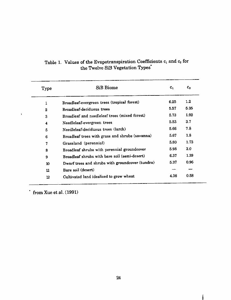
Table 1. Values of the Evapotranspiration Coefficients cl and c_ for
the Twelve SiB Vegetation Types*
Type SiB Biome cl Cs
1
2
3
4
5
6
7
8
9
10
11
12
Broadleaf-evergreentrees(tropicalforest) 6.25 1.2
Broadleaf-deciduoustrees 5.57 5.35
Broadleafand needleleaftrees(mixed forest) 5.73 1.92
Needleleaf-evergreentrees 5.53 3.7
Needleleaf-deciduous trees (larch) 5.66 7.8
Broadleaf trees with grass and shrubs (savanna) 5.67 1.8
Grassland (perennial) 5.80 1.73
Broadleaf shrubs with perennial groundcover 5.98 3.0
Broadleaf shrubs with bare soil (semi-desert) 6.37 1.39
Dwarf trees and shrubs with groundcover (tundra) 5.37 0.96
Bare soil(desert) --
Cultivatedland idealizedtogrow wheat 4.36 0.58
" from Xue et al. (1991)
24
HYDROLOGIC FIELDS: 10-Year Average of Monthly Means,
and Standard Deviations
Global distribution maps of key hydrologic fields are included in this
report. Ten-year (1979 - 1988) averages of the monthly mean precipitation,
evapotranspiration, root zone soil moisture, and runoff fields are plotted. In
addition, the standard deviations of the monthly mean precipitation,
evapotranspiration, root zone soil moisture, and runoff for the 10-year period
have been included.
25

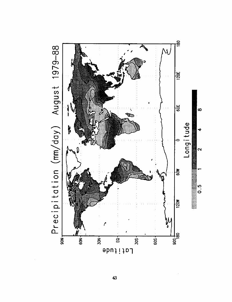
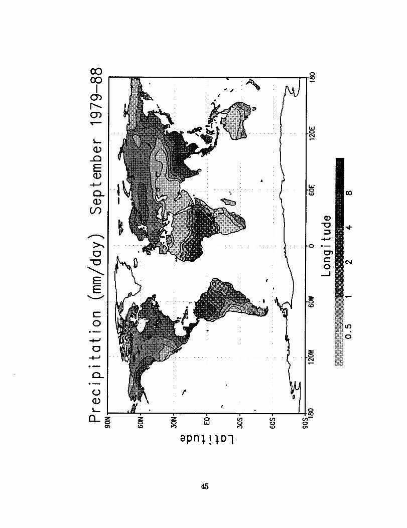
PRECIPITATION
(January - December)
Ten-year average (1979 - 1988) of the monthly mean precipitation (ram
day1), obtained from rain gage observations (Spangler and Jenne, 1990). Also
plotted are the standard deviations of the monthly mean fields as determined
from the 10-year data set.
27


CO00
IO_f.,,.
C_
C:
¢
Z0
apn_!
"0
o_
o,_J
29

>,,[:J
-O
EE
c-O
em
-I-,'
E_00"--(}{3
> I(1) O_
r'_ p,.
E_>-,-C3 _-EE3E3_
._, ¢-U')E_
c-O
o--
E_-4--'
em
r_Om
O(1)
a_
apn),!),D-I
Oo3
IJ.I
.o
I.i-o(D
.O e--
0._J
3)
oooOI
C_p-.(_
{D
_Q(PI,
apn_!),D-I
(-
o__J
QO
o_
_ .
iiil°::::::::::::::.:.:.:.:.:.:.:
31
-O
EE
c-O
0o_
om
Q_e_
0
L-
D_
hi
aPn_!_Dl
:3
Om
c-O
.J
32
00cO
IC_
C_
0k_
0
"0
EE
c-O
e_
0
eD
CI_e_
0(Dk...
13_
I .....
o
w
o
l.iJ-o
0oO
Z Z Z O" bO b_ 0"--0 0 0 bJ 0 0 0
aPn ! D7
en
t-
O
_i_ •iii!iiii!!iii_0
..-.....-.....?i:i:i:i:i:i:?iiii!iiiiiiii.:.:.:.:.:.:.:>:.:.:.:.:.:.
E3-13
EE
r-o
OI
E_"_(30
>00(DI
r_
{3-_..Er-- oE_l..
-_,E_
r-o
o_
E_
4bm
13.OD
O(D
apn_,!_,D7
0000I
C_r'-(_
m
el
L_
CL<c
n_
EE
(-O
On
Ou
CLWPm
O
CL
ZO
ZOco
\
_Pn_!_Ol
o_
(.-
O_J
35
EE
t-O
em
°_00
>00(_1
"{DO)
{D-IDm
_L•"_ O-c/') .,_:
c-O
e_
em
e_
(D
I,._
CL
apn),!),Dl
0000I
C_l'--C_
>.,
_E
>..,{D"O
EF:
v
c-
Oo_
{:D
o_
o_o_
CL
i .....
Z Z Z C_ _,_0 0 I._ 0 0
aPn)_!),D7
Q;
Om
t-
O._J
0nO
EE
V
c-
OOm
0Om
_00Q) O0
C_
-or'..L_c_
o,--no
O0
c-o
Om
0
em
O-em
(Jq)
13_
_)pn),!),Dl
0
38

v
_)pn),!),O'l
Q)
eD
r-0
._J
u_
iilidii!ii!iiiiii::
iliiiiiiii
19
0
EE
V
c-O
.0
!,--
0-0
or)
(-0
e_
{:}
e_
CLem
fO(D!._
13_
la.l
CD
(D"0
e_
(.-0
._1
:i:i:i:i:i:i:_:.:.:.:.:.:.:..:.:.:.:.:.:.::.:.:.:.:.:.:
c;
4O
00COI
C_
C_
m
v
+
\
_pn_!_Ol
o
00
w
Do
w-o_o
,0
(o
't'_l
D
000
(I)_-"0
(D"0
Om
0
41
EE_
v
c-O
Om
Om
C0
o_
om
Q_o_
(3_
z
epn !),D7
oOooI
C_r'-
CO
<I:
aPn),!),oq
Q)
e_
c-
O
00
4,3

EF:
V
(-..0
o_
_00
I,,,..
u').,_Z
(-
0el
Om
(..)
I,..
C}_
epn),!),Ol
O
.0 o_
t--0__I
00COI
O_P_C_'t""-
(D33
E(D
t_(DCO
Zorid
apn_!
o
_DI
_Jn_
.4-.'
OI
t-
O._3
Zo
o
I
i ......
t .....
\
.o
w-0¢o
-0
!
e_
c-O
46

oooo
IC_
(D
0
c_
¢
aPn_!_o7
"I0
Om
C
o__I
00
_T

EE
c-O
e_
---(_
>1
"0__-__0
0000
c-O
e_
e_
Q_o_
0
CL
Zo
apn),!),D-I
0
Om
0._1
0

00ooI
C_l'--C_
(I.)..Q
E(I.)>0
Z
_)pn),!),Dl
"O
o_
(-..
o__.I
4.9

"0
t=
._00
ql.-'-
I,-.I,,,,-
c-.Z
0ew
em
0
I,-
o
I.i.I
Bpn_.!),D'l
(L)"0
c-O

0000
IO'Jr_
t_
_O
E
q_
>,,C_
7O
EE
c-O
Om
C_
Om
O_om
O_ZOo_
oco
Zo
epn_! _O7
Q)
"0
Om
c-O
i,i,i,i,i,i,lio
_.............
51

"0
F:
V
c-
O
LI,,--
(._r'_
0,Im
0
om
om
L,.
Q_
0
_)pn_!),Dl
(D
Om
c-O.__I
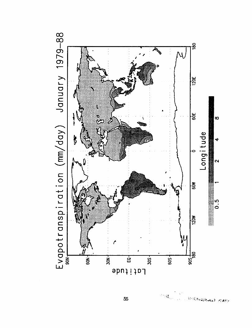
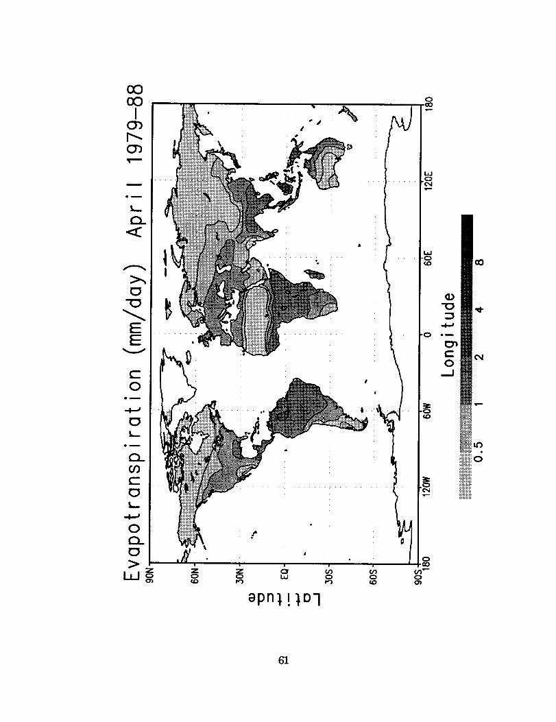
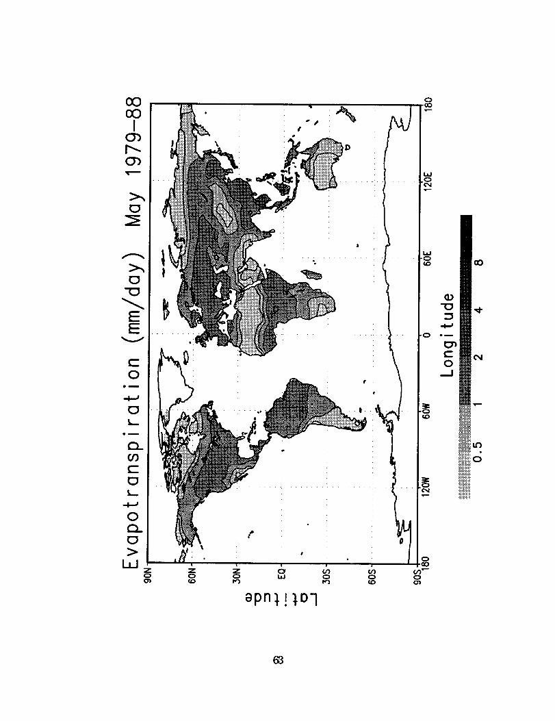
EVAPOTRANSPIRATION
(January - December)
Ten-year average (1979 - 1988) of the monthly mean evapotranspiration
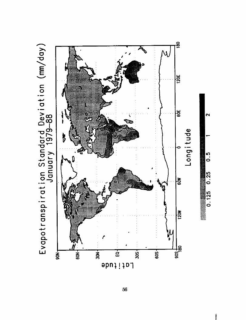
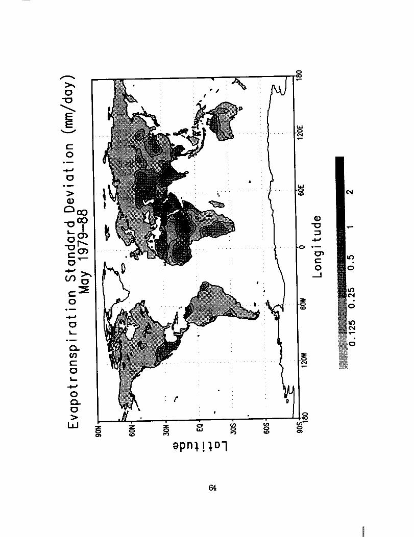
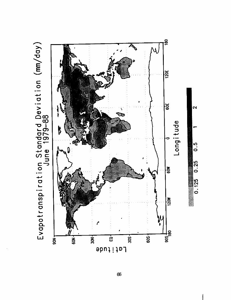
(mm day1), computed from soil moisture initialization scheme. Also plotted
are the standard deviations of the monthly mean fields as determined from the
10-year data set.
53

O0O0I
I"-.C_
:Dc-
¢
apn_! _07
I
w
,o
,0
I°/)q-"
0
'70
ol
c-O
,:,:,:,:,:.:.: 0
:.:.:.:.:.:.:.
!iiH
55 ._7_.. i :_ ,; _ . _ ......-...._ ..... ',_,,_._ _!_-.'_,.
0"0
E
t-O
o_
-i..a
0
_>
"0
Zo
zo
_pn_!_Dl
o
o
o-00
oo_
23
Ou
c-O
::::::::::::.:::::::.':.::
56

O0O0
IC_r--.c_
>,,
0
..QQ.)
L_
0"0
EE
O
0s._
Om
GOc-O
0
Ozo
LJ
!
apn_!_0q
.0
Q;
e_
c-
O_J
cO
c'N
::::::::::::::":':':':':':':0
:,'.:::::::::::::::::::::::::
Piiiiii!i!!!!i::::::::::::::
57

0
EE
V
0Om
0O!
0")
O_
o_
r_c-
O
¢
...... I
uJ
.o
"0
Om
O_t-O
._J
0

O0O0I
C_[-..(_
c-
OI,._
0
_E
-0
EE
Zo
apn_! ),07
"o:3
Om
(..-
o
::::::::::::::0
::::::::::::::
:,:.:.:.:.:.:.
iiiiiiiiiiil

apn_!_o7
i •
io
60
0000I
m
@D
t7
O
EE
c-O
e_
OL-
eD
C_
CO
OC_O
ZWo
.NO
ZO
Ow
0pn_!
0_o0
000
.0
000
0
<D
o_
t-o
_.J

........... "0 ei
\ oF
I-0
!
gpn),!),D'l
62
COCOI
C_P_C_
-0
EE
¢
aPn_!_ol
(D
:3
OR
c-
o_.I
..............::::::::::::::...............:.:.:<.:.>:::::::::::::::
iiiiiiiii!iiiiiiiiii_!_i!!!iii_iii_iiiiiii;.:.:.>:.>:.
0
63
O
EE
V
_pn),!},D-I
O
64

oooo
IC_
CT)
C
-D
>,,,
"0
EE
I
i
I
\, \
I
apn_!:Io-I
hl
o
I.,=1-0_o
.0
_o
0o(/i"--00')
W
¢i$!:!:i:_:::::::::::::::.:.:.:.:.:.:_:.:.:<.:.:.....o........::::::::::::::
65
EV
t-O
Om
Om
C_O0O0
-oi,L (3'}
4-,
(./3r-
t--'_0
o_
L.
o_
O.
t'-
0O_
I,I
....................... I
I
0ao
I
w
,0

oOO0
I
_ililili_i_iiio::_:i:i:!:i:i:
i_!!iiii_ii!ii
67
"0
EE
V
c-O
em
e_
>
r'_oOO0
_-C_
"O 0_c-_-
OOm
c--.._0
em
o_
O_coc-
OQ_
>L_
_pn),!),D-I

O0O0I
(3")r_.
(/3
<z:
_PnI!ID]
q)"o
em
o._J
ZO
.o
w
¢D
-0
"0
o_
C_(-.0
..._1
0
70
OOOOI
C_p...C_
_Q
E(P
CL(L)CO
"O
EF:
V
c-O
OI
{ZI)
OI
CL00
(--C)
O
LJ
#
_)Pn)!_O7
O
P
+i .....
I
w
o
C
o
'71
Bpn),!),Dl
w
B
r,o
o
_i_.i_: .
o
72
COO0
IO_I",-0")
..Q0
0C)
>,,CD
-0
EE
c--0
o_
Om
O_(/3c-_D
OO_
>oLLI
o
o
.o
"0¢0
0
-0
Io"_ (:_ _ O_ t,/) _'-0 W Q Q O
apnl!10-1
(D"o
mn
t-O
__1
>,,0
EE
t"0
em
r--L.--
-t.J
em
e_
(:1.U)(-.
t_
.4.J
0(:1.
>
epn),!),D-I

0000
IC_I"-.
(D..Ql=(D
OZ
EE
c-O
l,--
o_
00I::
O
_zO
I,Iapn_!_03
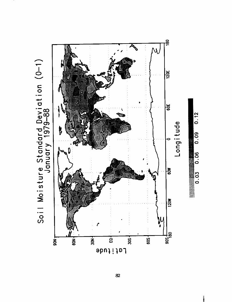
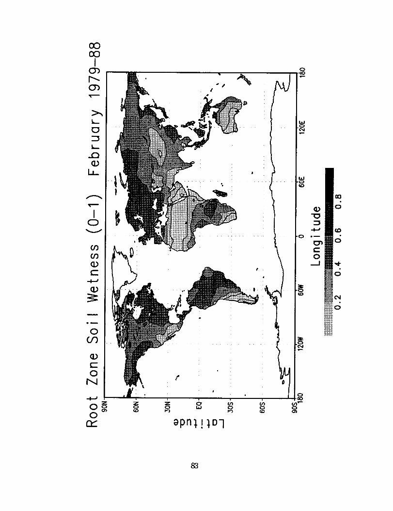
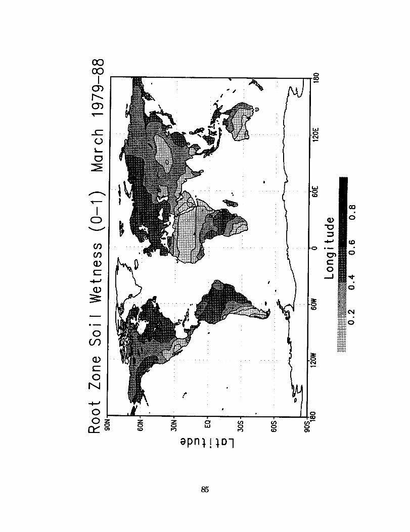
(D
Om
0__1
..,...........
iisl_:!_:._!:!:
75
EE
v
0,Jm
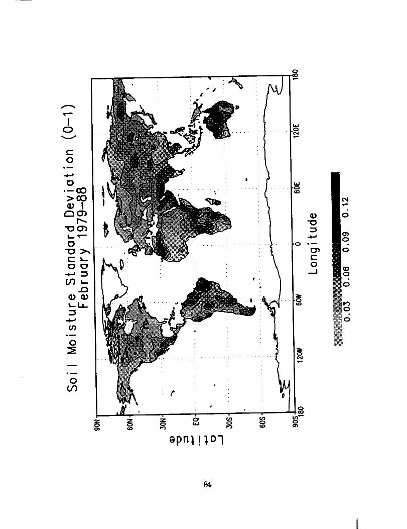
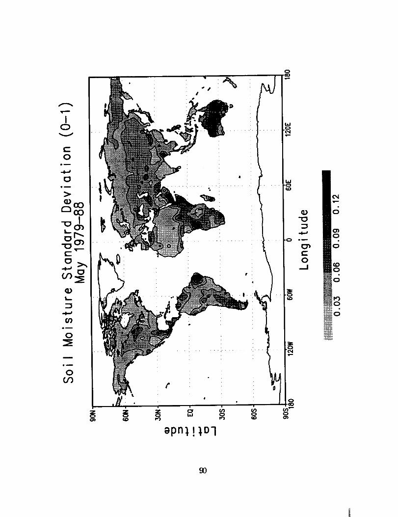
em
>00
r-,,l(_
"{_ r"-
('- L.
Or)I=(I)
O0
-m z
e_
(-,.
0
ILl Zo
l\\
' I
w
w
_D
.o
(1)
em
t-O
._.J6
6

O0O0
!0")r---c_
_QE(D0(D
aPn_!_Ol
0
0J 00
_.e')'"0
(D
:3
Om
c-O
_J
00
77
"O
EE
V
c-O
OU
CD'Died
a) oo
nD__..o_cD _--.-.
CDCD._..Q
f"OO_
.--g--_
o_
Q_toc-
O
I
0
_)pn),!),D'l
(D
Om
c-o__I
?8
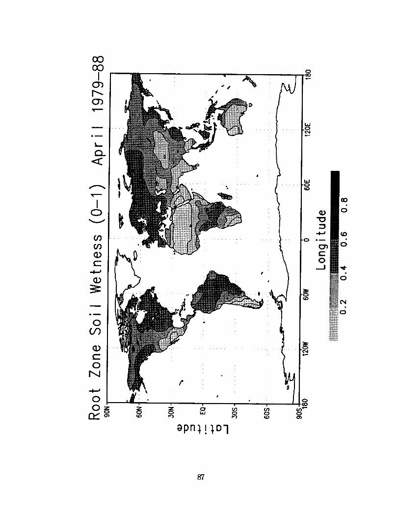
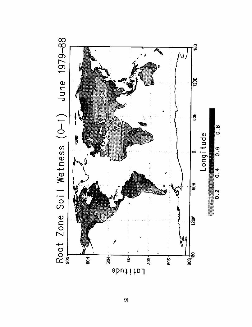
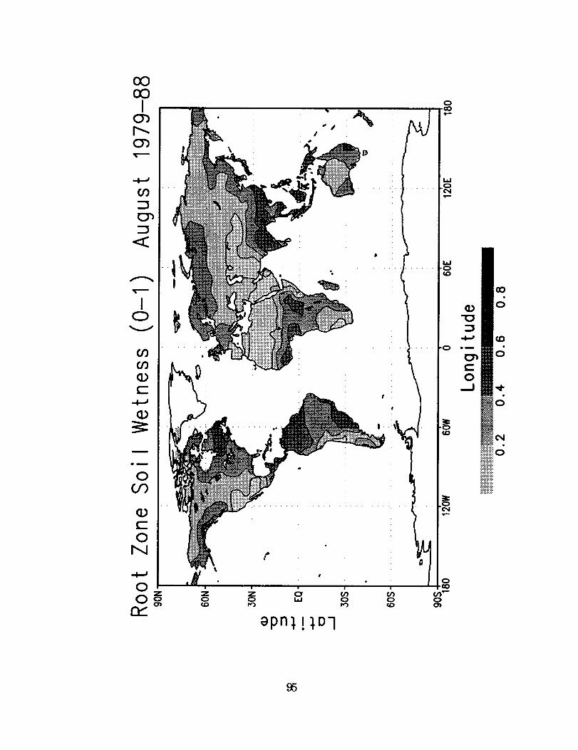
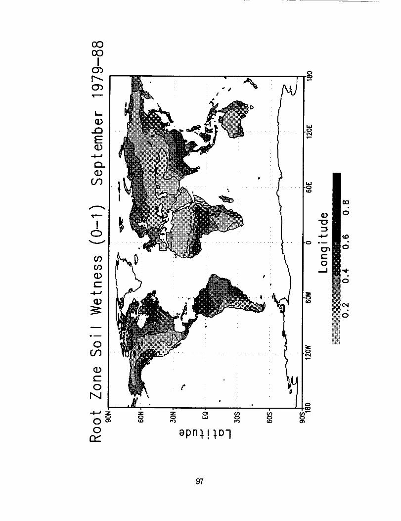
ROOT ZONE SOIL WETNESS
(January - December)
Ten-year average (1979 - 1988) of the monthly mean root zone soil
wetness (0 - 1), computed from soil moisture initialization scheme. Also
plotted are the standard deviations of the monthly mean fields as determined
from the 10-year data set.
79


O0O0I
CT)I'--CT)
>.,,
C3Z3
c--
E3
"-3
IC3
\
#
¢
_Pn_!_01
nO
eD
0._J
0
!o
81
i0V
I)
_)pn),!),Ol
82
CxDC_)I
C)')
0")
L
..Q
LL.
IC)
ZC)
:1o7
Q)
e_
Co
._J
00
C)
(Z)
6
o
0
16:.:.:.:.:.:.:.
88
m
eg
0(.I")
• 1 .....
q
Bpn_!),O'l
o_
t-O._J
-_.':::_i
_._:.
_C
BpnI!ID']
_o
_::::::::::..
_>:.:.:.:.:.:_;:_:::_

I0
em
o
Z0
I
|1 . .
b_D
pn ! Ol
o
w
o
0_0
r)_.-o
86
cO00
I
r_
em
O_<
I0
C
3_
el
0
t-O
N
0Oz
0 0
\
¢
Z0
c__!iiii!:_:!:i:i:i:!:
87

I0V
l,,_
Or) o_
I,,..
f_Om
0_E
I)
m
o_
0(])
0pn), !),O7
w
I
"¢_I
o
0
88

oOoO
IC_i"--C_
>,,
I0
g9
(DC
O
(Dc-O
N
OO
rt--o_ O
i
Zo
,:bi,i
apn_!
0
0
o
89
I0
v
0Ow
0o_
c-O
G)
f_Om
0
m
om
0_0
&
\
la.i
i,LI"0CO
"0
epn),!),ol
(D"0
.4,.,e
ew
(-.0.__I
0
0
0
90
w
.o
0
aPn:l.!),D'l
91

I0V
(-0
em
eu
r._0oI
_(_
(I)
f,_,Di
0_E
m
om
0or)
0
"O_J
o_
C7_
0_.J
0
0
o
0000I
O_
0")
I0
GOGOCDC
CD
m
ou
0Or)
¢l.)C0
N
00
rFo _o_
........... l •
\
apn_!_,o-I
OB
c-O
...I

I0V
c-
OOI
-l-a
Ou
¢)00r'_O0
I
"X_v--r-
,,l.am
--)
G)I,..
-l-a
(/)o_
0_E
m
om
0or)
ZO
ZO
.%
P
I ......
P
I .....
o
w
cD
,0
r,D
o_
0_.1
o
i_)c)
94
0000
IO_r--.o_
E_
<:
IO
E
(_
m
ou
OOr)
c-O
r,q
ooo _
r_aPn_!_Ol
I,i
-o{D
-O
n_
OR
e-0
QO
0
_Do
0
0
iii_!!!!iI_i
95

IC)
¢.-0
o_
om
>ao¢)ao
n l0")
_-0_
t'- .4-e
GO c::_
a)<
or)o_
0
m
om
0U')
Z0
Z0
I ......
\
0
la.l
i.I
,0 om
c-O
c;
0
0
96
ooooI
(_l'--C_
_0
F:(I)
CL
Or)
I0
0')Or)(Dc-
(I,)
em
0CO
(Dc-O
N
O
O o,O
rY
I,
........ ! ......
t
................. J....I
\\I
aPn)_!),O7
70
e_
(-.
o
:i:i-_..'.i:_::
,'.:._i:!:_:_:_
c;
(D
O
O,I
O
97

I0
V
0cO
_pn),!),Dl
0aO
0

O0O0I
p-.
_Q0
00
I0
m
OR
0Or)
ePn_!),oq
Z3
ew
t-O
co
o
o
o
I0V
c-
OQ_
.(_
0_E
B
o_
0Or)
ZQ
I)
ZQ¢D
...... 0
I,o0
(wO0co
JC_
"(",4
0aO
o0"-0
Bpn),!),DI
cO
C)
100

O0O0
I
_QE
>0
Z
I0
COO9q.)e-
/
em
0O0
c-O
N
ZOo
o')
0r'_
Zo
aPn_!]Ol
0
0
101

IO
c-O
o_
°_(_
>cO(DI
r'_o)r-,-
--o o-JL._ _r---
-,-, l=(f)(_
>
L..Z
,.4-"
U)Om
0
om
0(f)
epn),!),o-I

O0O0
I
_D
I0
O0
c-
Om
0O0
c-O
N
ZOo0
rY
0
P
I + • •
w
.o
Zo w
apn_!_oq
0 0 0
e_
t-O
o
I
V
c-
Oem
(DIr-_Cb
r'--•x_ 0"}
"C)_-
•-,-'I=O0(D
0
L_r'_
f,Oem
0_E
e_
0
I)
0
!!
_j
I .....
\
' 1
0cO
,,n
.o
104
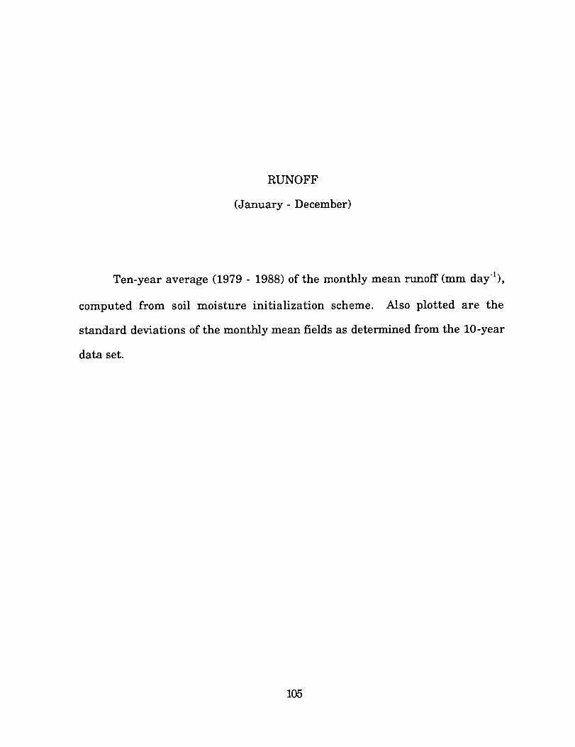
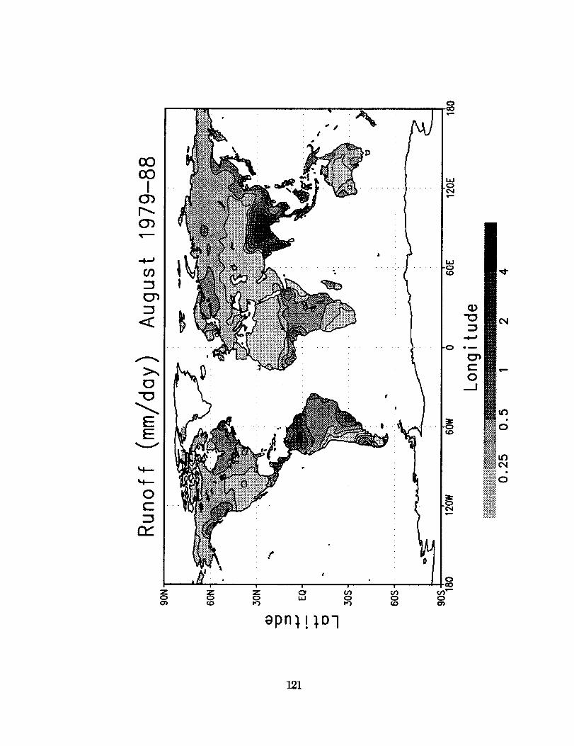
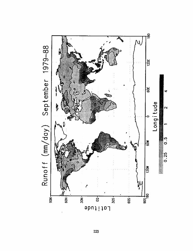
RUNOFF
(January- December)
Ten-year average (1979 - 1988) of the monthly mean runoff (mm day-l),
computed from soil moisture initialization scheme. Also plotted are the
standard deviations of the monthly mean fields as determined from the 10-year
data set.
105

oOoO
I
Zo
oPn_IlOl
.+
107 .............,."-_°, - " - ,..r._
0
s=E
V
:c&.0
_>,
r- .._)0
O0
0(,-.
rw"
0 0
0
108
oOoo
IC_r_
L_
_)Iu_
"O
EE
v
0r-
nl
0cO
w
,o
'C)¢.0
apn),!),D-I
¢)
eD
o
i!iii!ii!!!iliii!iiiiiiiiiii
iiiiii!iiiill
109
>,,
"O
EE
c-OOOOO
°_ i
_ I",-°_O')
qZ_t-_ >,,
"O (:3
"O..Q
OLI..-i.-a
C_O
OCZ_
BPn_!_DI
"O
-i..a
eu
O._.1
O4
Le_
c_
ICJ
O
.:;_._
NN o48i:i:-:_:!:i
110
0000
I0")!'--0"}
c-O
_E
>.,
x:)
EE
4--
,,¢-.
0(.-
rY
Z
la.I
BPni!_D1
111
EE
V
c-
eB
r.o
U_)
0¢-.
n_
_)pn),!),O'l
(1)
4.Je_
t-O
._Jc;
C)
O0O0
I
I"--C_
m
oD
Q_<C
apnl!_o-I
w
o
-0¢0
Q_
o_
c-O_J
113
V
0(,-.
0"
Z
_)pnl !),O'l
e_
0
0
LO
i,,'-
::::::::::::::
iii!iiiiiiili:.:.:,:.:<.:.
114

O0COI
C_p-.C_
0
0
-0
EE
0r-
r_
Z0
.No
z o _ w0 ILl 0 0rO rO _D
o
0pn)!_Ol
w
.o
w-0
,0
-o(o
o/)'--0O_
el)
Om
0_.J
0
_iiiiiiiiiiiiioi_ii!iiiiiiiii
aPnl!ID'l
116
CO00I
C_p..0")
c-
-0
EE
0C
P_
Z Z Z (3r GO bO0 0 0 b.J 0 0
aPn_!_Ol
117

"IO
EE
t'-O
°_
.._00
>r-,,q.) (3')
-o q)
-o'-_
(3
U3
O
rY
ZO
q)"IO::3
Om
t-O
_J
C)
0000I
O_
O_
m
"O
t::E
O(.--
D
G.)"O
OD
r--o
._I
_pn_! _o7
119

>,,C_
EE
V
c-O
-_(_)
-_ (:X_o l
"_ >,,L.u
(.-
(._
4...
0c"::3
r_
Bpn),!),Ol
o
w
w
f.D
-o
(1)"0
em
c-O
__1
0
iiiiiiiii_iiil
120
ooO0I
C_I'--0")
O0
<C
w
&,_.o
.0
_)pn_!]Dl
OR
(.-.0._.J
&C}e
0
c_
ii.-'iiiiiii_iii
121
G_
EE
V
c-
OO0
"-'I_ (:}')
o_
Q) .,--
"O CO
"ID :::}(-._:C:)
Or)
NI--
Nl,--
0c-::3
rY
Z0o_
_Z0
aPn1!_D1
(I)"xD::}
OI
C:_c-O.._I
I0
::::::::::::;:•
122
0000I
0")
oE.=l_a
Or)
oct,"
Zo
o
i,i
.o
o
o0
0
aPn),!_O7
opn),!),O-I
124
O0O0I
D_(_
Q_c_0
(o0
0
EE
0c--
n-
Z0
zoco
_pn_!_Ol
125
O0
0ooS..D
bJ
o
ILl'0
"0
apn),!),D7
0
126

O0O0I
C_r_c_
L..
(I)_QE(i.)
0Z
v
\
i .....
_)pn1!),D-I
O.)-io:::}.4,,-,o_
(.-
o.__I
I0
i!iiiiiiiiiii!iii(:;.:.:,:,:,:.:.:.:.:,:.:,:,:.:i!i_i_iiiiiiii
iliJii!iiiii!
127

O
EE
V
r-0oo0o
.4.., (3bor--.
r-_(1)
-_..oL-E0 (!,)
nO_>,t"OOZ
Or)
Or-
OC
w
W.of,D
,-0
(1)nO
o_
t-O
__10
_.:i::.;i:i:E:
128
O0O0
I
E
q_r7
C_
EE
v
4--
4--
0c-
Z0
,P
apn_! 1o7
i
i .....
I .....
W
W"0
O"O
EE
V
r-0oo0o
-_,C_
°_C_
(Dr'_L_
(D
"O..Q
L-EO(1)
00
O
_3
n_"
ZO
io
130

Form Approved
REPORT DOCUMENTATION PAGE OMBNo. O704-0188
Public reporting burden for thiscollection of information is estimated to average 1 hour per response, includingthe time for reviewinginstructions, searching existing data sources,gathering and maintaining the data needed, and completing and reviewing the collection of information. Send comments regarding this burden estimale or any other aspect of thiscollection of information, includingsuggestionsfor reducingthis burden, to WashingtonHeadquarters Services,Directorate for Information Operations and Reports, 1215 JeffersonDavis Highway. Suite 1204, Arlington, VA 22202-4302. and to the Office of Management and Budget, Paperwork ReductionProject (0704-0188). Washington, DC 20503.
1, AGENCY USE ONLY (Leave blank) 2. REPORT DATE 3. REPORT TYPE AND DATES COVERED
August 1993 Technical Memorandum4. TITLE AND SUBTITLE 5. FUNDING NUMBERS
Design of a Global Soil Moisture Initialization Procedure fort.he
Simple Biosphere Model
6. AUTHOR(S)
G. E. Liston, Y. C. Sud, and G. K. Walker
7. PERFORMING ORGANIZATION NAME(S) AND ADDRESS (ES)
Goddard Space Flight Center
Greenbelt, Maryland 20771
9.SPONSORING/ MONITORINGADGENCYNAME(S)ANDADDRESS(ES)
National Aeronautics and Space Administration
Washington, DC 20546-0001
JON-910-039-09-01-25
8. PEFORMING ORGANIZATION
REPORT NUMBER
93B00092
10. SPONSORING / MONITORING
ADGENCY REPORT NUMBER
NASA TM-104590
11.SUPPLEMENTARYNOTES
G. E. Liston, Universities Space Research Association, Columbia, MD; Y. C. Sud, Goddard Space
Flight Center, Greenbelt, MD; G. K. Walker, General Sciences Corporation, Laurel, MD
12a.DISTRIBUTION/ AVAILABILITYSTATMENT 12b.DISTRIBUTIONCODE
Unclassified - Unlimited
Subject Category 47
13. ABSTRACT (Maximum 200 words)
Global soil moisture and land-surface evapowanspiration fields are computed using an analysis scheme based on the
Simple Biosphere (SiB) soil-vegetation-amaosphere interaction model. The scheme is driven with observed precipi-
tation, and potential evapotranspiration, where the potential evapowansph'afion is computed following the surface air
t_-potential evapotranspirafion regression of Thomthwaite (1948). The observed surface air temperature is
conected to reflect potential (zero soil moisture stress) conditions by letting the ratio of actual transpiration to poten-
tial transpiration be a ftmction of normalized difference vegetation index (NDVI). Soil moisture, evapotranspiration,
and runoff data are generated on a daily basis for a 10-year period, January 1979 through December 1988, using
observed precipitation gridded at a 4° by 5° resolution.
14. SUBJECT TERMS
Soil moisture, Precipitation, Evapotranspirafion, Runoff, GCM initial conditions
17. SECURITY CLASSIFICATIONOF REPORT
Unclassified
NSN 7540-01-280-5500
18. SECURITY CLASSIFICATIONOF THIS PAGE
Unclassified
19. SECURITY CLASSIFICATIONOF ABSTRACT
Unclassified
15. NUMBER OF PAGES
]3816. PRICE CODE
20. UMITATION OF ABSTRACT
UL
Standard Form 298 (Rev. 2-89)Prescribed by ANSI Std. Z39.18298-102


National Aeronautics and
Space Administration
Goddard Space Flight CenterGreenbelt, Maryland 20771
Official Business
Penalty for Private Use, $300
SPECIAL FOURTH-CLASS RATE
POSTAGE & FEES PAID
NASA
PERMIT No. G27
POSTMASTE R: If Undeliverable (Section 158,
Postal Manual) Do Not Return