Embed Size (px)
Citation preview
Design of a Scaled Down Acoustic Experiment with
Anechoic and Reverberation Chambers
Undergraduate Honors Thesis
Presented in Partial Fulfillment of the Requirements for
Graduation with Distinction in the
Department of Mechanical Engineering at
The Ohio State University
By:
Eric D. Ricciardi
Advisors: R. Singh, Mechanical Engineering, [email protected]
J. Dreyer, Mechanical Engineering, [email protected]
******
The Ohio State University
March 2013
Defense Committee:
Dr. Rajendra Singh
Dr. Jason Dreyer
Dr. Brian Harper
1 | R i c c i a r d i
Abstract
The focus on this research is to design and evaluate a split chamber that can be used for
measuring random incidence properties of acoustic materials and achieve reliable results for
frequencies larger than 500 Hz. A split chamber consists of an anechoic section and a reverberant
section; therefore the sound field in each portion must be designed to simulate direct and diffuse
field conditions in the far field. The challenge in this test chamber design is adhering to small
scale dimension constraints of 2.4m x1.2m x 1.2m and a maximum cost of $1000, while
maintaining a certain level of performance in terms of lowest frequency that can be
characterized. By analyzing both acoustical field theory and absorption characteristics this
chamber is found to have a cutoff frequency of approximately 570 Hz. The far field sound
pressure distribution in the reverberant chamber was determined to be sufficiently uniform, both
in the room and across the panel. Sound pressure measurements in the anechoic chamber
correlated well to the inverse square law, given by ideal direct field conditions. The noise
reduction of the room to the outside ranged from 27 dB to 40 dB across the designed frequency
range, which indicates that the chamber is sufficiently sealed from the ambient sound. The
chamber was built to be within the sizing constraints and met a final construction cost under
$1000. This split chamber will be used to assist in student projects and as a teaching tool for
mechanical engineering courses. Future work on this project will consider the addition of
diffusers in the reverberant chamber; this study will be done using boundary element modeling
software and experimental measurements.

2 | R i c c i a r d i
Table of Contents
Acknowledgements .....................................................................................................................................................................3
List of Figures .................................................................................................................................................................................4
Chapter 1: Introduction .............................................................................................................................................................6
1.1 Background .........................................................................................................................................................................6
1.2 Significance of Research ...............................................................................................................................................9
1.3 Project Formulation and Scope ............................................................................................................................. 10
Chapter 2: Design/Fabrication ........................................................................................................................................... 11
2.1 Design Considerations/Constraints .................................................................................................................... 11
2.2 Proposed design ............................................................................................................................................................ 14
2.4 Construction .................................................................................................................................................................... 16
2.6 Final Chamber ................................................................................................................................................................ 18
Chapter 3: Theoretical Considerations ........................................................................................................................... 19
3.1 Direct and Diffuse Field Theory ............................................................................................................................ 19
3.2 Room Modes .................................................................................................................................................................... 21
3.3 Surface Interaction (Absorption) ......................................................................................................................... 24
3.4 Surface Interaction (Transmission) .................................................................................................................... 27
3.5 Evaluation Criterion .................................................................................................................................................... 28
3.5 IL, TL, Test Method ................................................................................................................................................. 29
Chapter 4: Experimental Evaluation................................................................................................................................ 31
4.1 Testing Set-Ups .............................................................................................................................................................. 31
4.2 Cutoff Frequency and Absorption Measurements ....................................................................................... 36
4.3 Uniform Pressure Evaluation (Reverberation Chamber) ........................................................................ 38
4.4 Transmission Loss Measurements ...................................................................................................................... 42
Chapter 5: Conclusions ........................................................................................................................................................... 46
5.1 Conclusion ........................................................................................................................................................................ 46
5.2 Sources of Error ............................................................................................................................................................. 47
5.3 Recommendations for Future work .................................................................................................................... 48
Appendix ........................................................................................................................................................................................ 50
References ..................................................................................................................................................................................... 52
3 | R i c c i a r d i
Acknowledgements
I would like to thank all of the individuals that have provided support and guidance over the
course of this project. I would like to acknowledge Dr. Rajendra Singh, Dr. Jason Dreyer, and
Dr. Brian Harper for their service in my defense committee and the guidance and critique they
offered. I would like to thank the Acoustics and Dynamics Laboratory and the Department of
Mechanical Engineering at The Ohio State University for the use of their facilities and other
resources. Finally, a special thanks to The Undergraduate Honors Committee in the College of
Engineering for the financial support awarded during the duration of this project.
4 | R i c c i a r d i
List of Figures
Figure 1: Normal Sound Incidence ...........................................................................................................................................7
Figure 2: Random Sound Incidence..........................................................................................................................................7
Figure 3: Impedance Tube Method [11] ................................................................................................................................8
Figure 4: Example of Full Scale Split-Chamber [10] ..................................................................................................... 11
Figure 5: Anechoic Room [10].................................................................................................................................................. 13
Figure 6: Wireframe Solidworks Model .............................................................................................................................. 14
Figure 7: Reverberant Chamber Design .............................................................................................................................. 15
Figure 8: Anechoic Chamber Design ..................................................................................................................................... 15
Figure 9: Installing Casters ........................................................................................................................................................ 16
Figure 10: Building Frame ......................................................................................................................................................... 16
Figure 11: Caulking the Seems ................................................................................................................................................. 16
Figure 12: Sealant and Clamps ................................................................................................................................................. 16
Figure 13: Mounted Panel (25 Mic Array) ......................................................................................................................... 17
Figure 14: Installing Sample Mount ...................................................................................................................................... 17
Figure 15: Installing Foam ......................................................................................................................................................... 17
Figure 16: Foam Wedges ............................................................................................................................................................ 17
Figure 17: Reverberation Chamber ....................................................................................................................................... 18
Figure 18: Both Chambers (Open) ......................................................................................................................................... 18
Figure 19: Inside of Anechoic Chamber .............................................................................................................................. 18
Figure 20: Anechoic Chamber .................................................................................................................................................. 18
Figure 21: Definition of Reverberation Time ................................................................................................................... 20
Figure 22: An Example of Ray Tracing from the Source ............................................................................................. 21
Figure 23: Schematic of Outer Wall With Panel .............................................................................................................. 23
Figure 24: Normal Room Modes ............................................................................................................................................. 24
Figure 25: Practical Average Absorption Values ............................................................................................................ 25
Figure 26: Absorption Test Method ...................................................................................................................................... 29
Figure 27: TL and IL Test Method .......................................................................................................................................... 30
Figure 28: Mounted Power Source ........................................................................................................................................ 32
Figure 29: Sealed Anechoic Chamber ................................................................................................................................... 32
Figure 30: Anechoic Microphone Set-up ............................................................................................................................ 32
Figure 31: Vibration Idolaters .................................................................................................................................................. 33
Figure 32: Reverberation Chamber Microphone Set-up ............................................................................................ 33
Figure 33: Speaker Set-Up .......................................................................................................................................................... 34
Figure 34: Microphone Array ................................................................................................................................................... 34
Figure 35: Coordinate Definition ............................................................................................................................................ 35
Figure 36: Microphone Placement ......................................................................................................................................... 35
Figure 37: Panel with ¾” Diameter Air Gap...................................................................................................................... 35
Figure 38: Background Noise ................................................................................................................................................... 36
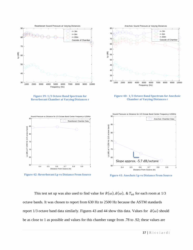
Figure 39: 1/3 Octave Band Spectrum for Reverberant Chamber at Varying Distances r ....................... 37
Figure 40: 1/3 Octave Band Spectrum for Anechoic Chamber at Varying Distances r ............................. 37
Figure 41: Anechoic Lp vs Distance From Source .......................................................................................................... 37
5 | R i c c i a r d i
Figure 42: Reverberant Lp vs Distance From Source .................................................................................................. 37
Figure 43: Table of Values for Anechoic Chamber ........................................................................................................ 38
Figure 44: Table of Values for Reverberation Chamber ............................................................................................. 38
Figure 45: Total Sound Pressure Profile on Panel ......................................................................................................... 39
Figure 46: Deviation from Average Pressure on Panel ............................................................................................... 39
Figure 47: 1/3 Octave Band Frequency Spectrum for all 25 Microphones ...................................................... 40
Figure 48: 25 Microphone Array 1/3 Octave Band Frequency Spectrum Near Cutoff Frequency ...... 40
Figure 49: 1/3 Octave Band Frequency Spectrum Near Cutoff Frequency for Various Points in the
Room ..................................................................................................................................................................................................... 40
Figure 50: 1/3 Octave Band Frequency Spectrum for Various Points in the Room..................................... 40
Figure 51: Table of Total Sound Pressure Levels at Various Points in the reverberant Chamber ....... 41
Figure 52: Noise Reduction of Room (to Outside) ......................................................................................................... 42
Figure 53: Plot of TL at Varying Air Gaps ........................................................................................................................... 43
Figure 54: Table of TL, IL, and NR for Varying Air Gaps ............................................................................................. 43
Figure 55: TL Potential for % Air Opening [14] .............................................................................................................. 44
Figure 56: Table of TL Data at 1250 Hz ............................................................................................................................... 44
Figure 57: Comparing Theoretical and Experimental TL .......................................................................................... 45
6 | R i c c i a r d i
Chapter 1: Introduction
1.1 Background
Acoustic materials are used in a wide range of applications in industry, from small scale
product design to large scale construction applications. Investigation of acoustic properties is
often implemented in the design process of enclosed environments. Generally, objectives of this
investigation can fit into one of three classifications: noise control, music perception/enjoyment,
or speech intelligibility. Each of these classifications requires a different approach to the design
problem and the choice of acoustic treatment. There are a wide range of acoustic properties
available on the market and it is valuable to be able to characterize these materials in order select
the best material for a given design problem. The acoustic properties of materials to be quantified
by this test apparatus are: absorption coefficient (), transmission loss (TL) and insertion loss
(IL). Noise reduction (NR) and sound transmission class (STC) are also often reported but have
little scientific meaning. These properties can be measured for a panel of a given material or of
an enclosure. For applications involving music perception/enjoyment or speech intelligibility
is the dominating acoustic property. Likewise, for noise reduction applications, TL and IL are the
dominating properties to be considered. There are several methods for determining these
properties. This research focuses on random sound incidence properties of materials, which
requires a split-chamber design to characterize panel treatments.
Acoustic properties of materials can be characterized by using either random sound
incidence or normal sound incidence. Figure 1 illustrates normal sound incidence; the initial
sound is the sound originating from a sound source, this sound comes in contactwith the solid
material at a 90° angle (normal) and is reflected/transmitted in the normal direction. Normal
sound incedence test methods include sound only in the normal direction.

7 | R i c c i a r d i
Figure 1: Normal Sound Incidence
However in many real world applications sound approaches at many different angles. Figure 2
illustrates the concept of random sound incedence. The initial sound approaches at various angles
and is reflected/transmitted at various angles. Snell’s law can be used to describe the relationship
between the agnels of incedence and refraction.
Figure 2: Random Sound Incidence
Bench-top devices, such as impedance tubes, used to characterize acoustic material
properties exist, but assume plane waves and are therefore restricted to study normal sound
8 | R i c c i a r d i
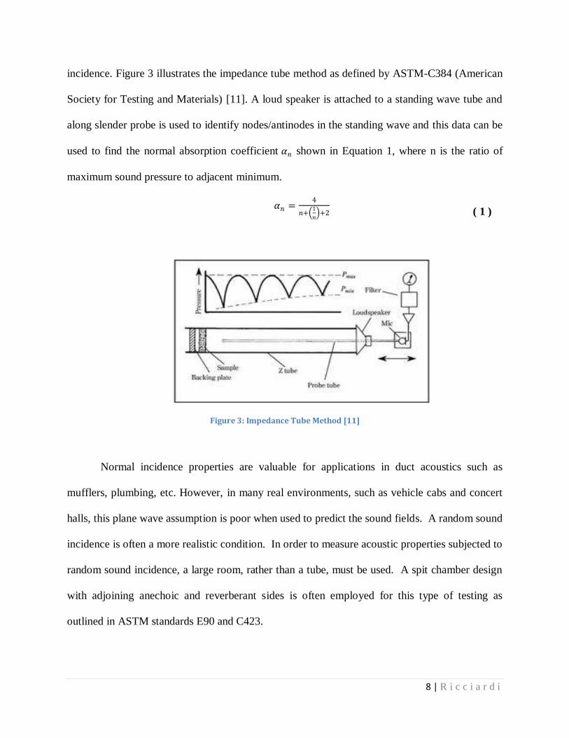
incidence. Figure 3 illustrates the impedance tube method as defined by ASTM-C384 (American
Society for Testing and Materials) [11]. A loud speaker is attached to a standing wave tube and
along slender probe is used to identify nodes/antinodes in the standing wave and this data can be
used to find the normal absorption coefficient shown in Equation 1, where n is the ratio of
maximum sound pressure to adjacent minimum.
(
)
Figure 3: Impedance Tube Method [11]
Normal incidence properties are valuable for applications in duct acoustics such as
mufflers, plumbing, etc. However, in many real environments, such as vehicle cabs and concert
halls, this plane wave assumption is poor when used to predict the sound fields. A random sound
incidence is often a more realistic condition. In order to measure acoustic properties subjected to
random sound incidence, a large room, rather than a tube, must be used. A spit chamber design
with adjoining anechoic and reverberant sides is often employed for this type of testing as
outlined in ASTM standards E90 and C423.
( 1 )
9 | R i c c i a r d i
1.2 Significance of Research
The Acoustic and Dynamics Laboratory (ADL) at The Ohio State University currently
has a working test set-up for characterizing normal incidence properties of acoustic materials, but
there exists no such set-up for random sound incidence; any such testing must be done in an
outside laboratory. As previously noted, there is significant real world application for random
incidence properties and this project will provide the means to test these properties. The split-
chamber constructed and evaluated as a result of this project can be used for industry sponsored
projects as well as a valuable teaching tool for undergraduate and graduate students. This split-
chamber will possibly be used for laboratory experiments in acoustics courses offered through
the Mechanical Engineering Department.
The applications of random sound incidence are mostly for studying the effects of panel
treatments in different rooms; lecture halls, concert halls, recording studios, etc. When
considering acoustics in the design of a room, it is also valuable to be able to characterize the
sound field within that room. Characterization of a room includes estimating direct field and
diffuse field contributions; which involves quantifying how much of the sound you are hearing is
directly from the sound source (direct field) and how much has been reflected from a surface
within the room (diffuse field). Often, these field contributions are estimated during the design
process and evaluated after construction. The split-chamber design considered in this project
includes a completely anechoic room (direct field) and a completely reverberant room (diffuse
field). In order to design/evaluate this split-chamber the fields in each room must be
characterized with a similar method used in real world construction applications.
10 | R i c c i a r d i
1.3 Project Formulation and Scope
The main deliverable of this research is to develop a small-scale acoustic test chamber
(spit chamber design) that can be used to characterize acoustic properties of panel treatments
subjected to random sound incidence. ASTM standards E90 [2] and C423 [3] will be used as
references to construction and testing procedures. Those standards describe the type of enclosure
and test method used to characterize random incidence properties of materials. ASTM E90 and
C423 refer to the “Standard Test Method for Laboratory Measurement of Airborne Sound
Transmission Loss of Building Partitions and Elements” and the “Standard Test Method for
Sound Absorption and Sound Absorption coefficient by the Reverberation Room Method”
respectively. The objectives of this project are:
i) Design of small scale split-chamber and determination of materials needed.
ii) Fabrication of the design.
iii) Evaluation of test chamber and report of cutoff frequency (lowest reliable
frequency for measurements).
This project should yield a working chamber with a defined test method to measure IL,
TL and . This chamber should be useful for frequencies above 500 Hz, the actual value of the
chamber will be measured. The scope of this project requires both computational and
experimental components. Transmission phenomena will be studied in the calculation and
measurements of , and one for TL and IL. Acoustic field theory will be used to characterize the
field within the anechoic and reverberant rooms. Experimental results will be compared to the
theoretical calculations for transmission phenomenon and acoustic field theory. This project will
conclude with suggestions for improvements on the design and further study using this split-
chamber.
11 | R i c c i a r d i
Chapter 2: Design/Fabrication
2.1 Design Considerations/Constraints
The major challenge in the design of this split-chamber is to adhere to ASTM standards
as closely as possible while adhering to sizing and budget constraints. ASTM E90 describes
standards for the construction of such a chamber [2]. These chambers are reliable for frequencies
above 200 Hz and are generally 125 to 300 m3
in volume, and require a sample size of 1 m2;
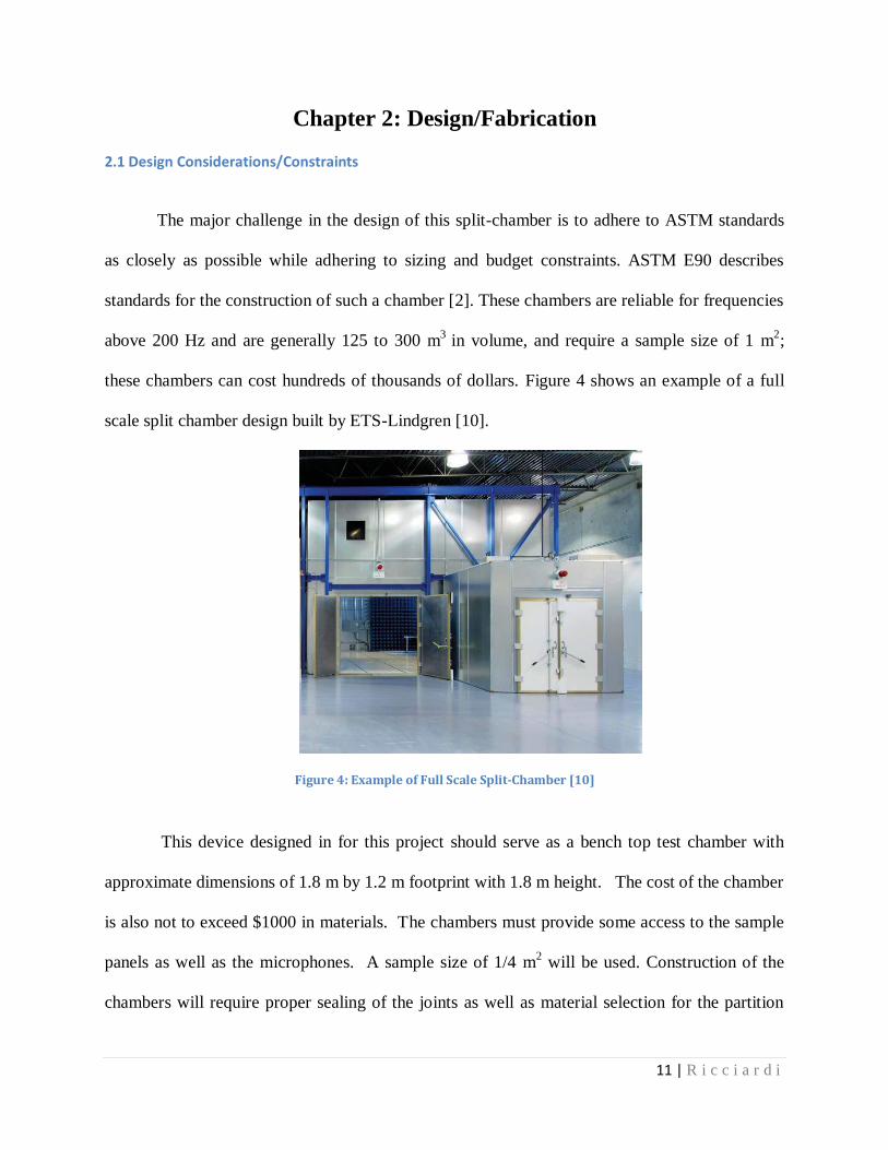
these chambers can cost hundreds of thousands of dollars. Figure 4 shows an example of a full
scale split chamber design built by ETS-Lindgren [10].
Figure 4: Example of Full Scale Split-Chamber [10]
This device designed in for this project should serve as a bench top test chamber with
approximate dimensions of 1.8 m by 1.2 m footprint with 1.8 m height. The cost of the chamber
is also not to exceed $1000 in materials. The chambers must provide some access to the sample
panels as well as the microphones. A sample size of 1/4 m2 will be used. Construction of the
chambers will require proper sealing of the joints as well as material selection for the partition
12 | R i c c i a r d i
materials, such as medium density particle board, in order to reduce unmeasured transmitted
sound into or out of the chambers.
Reverberation chamber sizes defined in the ASTM specifications are a minimum of 125
m3 in volume. The volume and length requirements of the chamber is recommended to be
greater than 43 and a major dimension greater than 1.5, where is the wavelength in m of the
lowest frequency in Hz of interest to be measured. Reverberant chambers are usually constructed
from hard rigid walls to reflect virtually all of the sound. The challenge in designing and
building a reverberant chamber is to reduce break up enclosure modes, also referred to as
standing waves. Many different physical apparatuses can be used to minimize standing waves
such as: diffusers, large rotation reflective vones (a fan like object), and warble tones or random
noise generators [4]. In addition, the walls of these chambers are often constructed at different
adjoining angles to reduce parallel and perpendicular surfaces. The crucial feature of a
reverberant chamber is that the sound pressure level readings are uniform throughout the
chamber; this will be observed so long as there are minimal standing waves. Measurement
techniques often include multiple microphones placed at different locations within the chamber
or a single microphone may be placed on a rotating boom and the measurement becomes
spatially averaged as the traveling microphone data is time averaged.
Anechoic chambers are designed to accommodate the maximum absorptive treatment
while still allowing for a sample to be placed within the chamber. In the case of panel
characterization, almost all of the volume reserved for the anechoic chamber can be devoted to
absorptive materials as the panel will only be placed on the wall adjoining the two chambers.
This is an effective design as long as the wall treatments do not interact with the panel sample.
The lowest effective frequency for the anechoic chambers is often dictated by the thickness of
13 | R i c c i a r d i
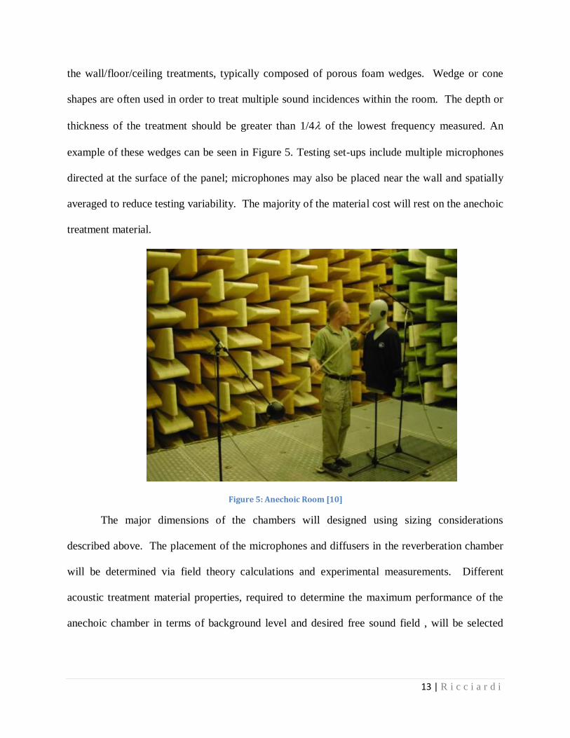
the wall/floor/ceiling treatments, typically composed of porous foam wedges. Wedge or cone
shapes are often used in order to treat multiple sound incidences within the room. The depth or
thickness of the treatment should be greater than 1/4 of the lowest frequency measured. An
example of these wedges can be seen in Figure 5. Testing set-ups include multiple microphones
directed at the surface of the panel; microphones may also be placed near the wall and spatially
averaged to reduce testing variability. The majority of the material cost will rest on the anechoic
treatment material.
Figure 5: Anechoic Room [10]
The major dimensions of the chambers will designed using sizing considerations
described above. The placement of the microphones and diffusers in the reverberation chamber
will be determined via field theory calculations and experimental measurements. Different
acoustic treatment material properties, required to determine the maximum performance of the
anechoic chamber in terms of background level and desired free sound field , will be selected
14 | R i c c i a r d i
from catalog values, but will their performance will be quantified with measured valued after
mounted.
2.2 Proposed design
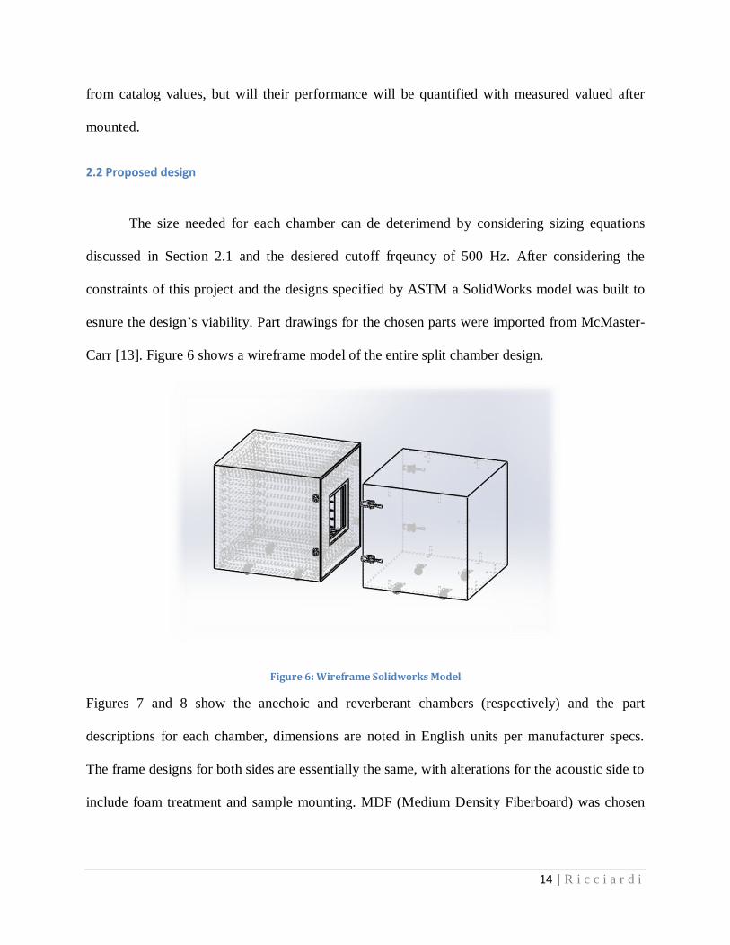
The size needed for each chamber can de deterimend by considering sizing equations
discussed in Section 2.1 and the desiered cutoff frqeuncy of 500 Hz. After considering the
constraints of this project and the designs specified by ASTM a SolidWorks model was built to
esnure the design’s viability. Part drawings for the chosen parts were imported from McMaster-
Carr [13]. Figure 6 shows a wireframe model of the entire split chamber design.
Figure 6: Wireframe Solidworks Model
Figures 7 and 8 show the anechoic and reverberant chambers (respectively) and the part
descriptions for each chamber, dimensions are noted in English units per manufacturer specs.
The frame designs for both sides are essentially the same, with alterations for the acoustic side to
include foam treatment and sample mounting. MDF (Medium Density Fiberboard) was chosen
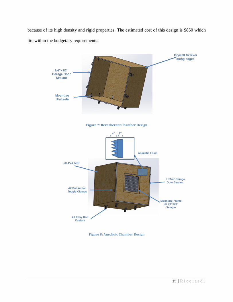
15 | R i c c i a r d i
because of its high density and rigid properties. The estimated cost of this design is $850 which
fits within the budgetary requirements.
Figure 7: Reverberant Chamber Design
Figure 8: Anechoic Chamber Design
16 | R i c c i a r d i
2.4 Construction
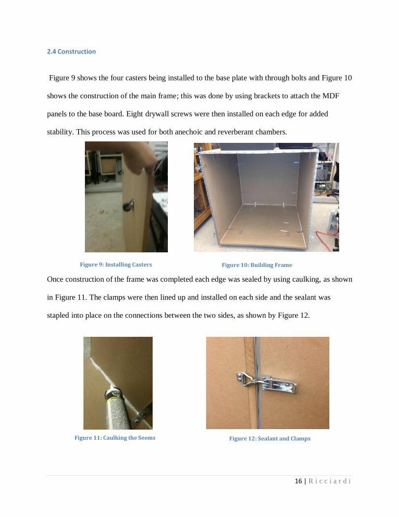
Figure 9 shows the four casters being installed to the base plate with through bolts and Figure 10
shows the construction of the main frame; this was done by using brackets to attach the MDF
panels to the base board. Eight drywall screws were then installed on each edge for added
stability. This process was used for both anechoic and reverberant chambers.
Once construction of the frame was completed each edge was sealed by using caulking, as shown
in Figure 11. The clamps were then lined up and installed on each side and the sealant was
stapled into place on the connections between the two sides, as shown by Figure 12.
Figure 10: Building Frame Figure 9: Installing Casters
Figure 12: Sealant and Clamps Figure 11: Caulking the Seems
17 | R i c c i a r d i
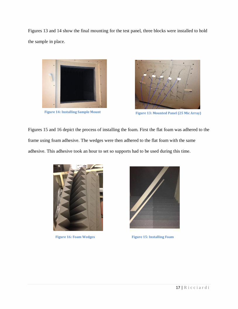
Figures 13 and 14 show the final mounting for the test panel, three blocks were installed to hold
the sample in place.
Figures 15 and 16 depict the process of installing the foam. First the flat foam was adhered to the
frame using foam adhesive. The wedges were then adhered to the flat foam with the same
adhesive. This adhesive took an hour to set so supports had to be used during this time.
Figure 13: Mounted Panel (25 Mic Array) Figure 14: Installing Sample Mount
Figure 15: Installing Foam Figure 16: Foam Wedges
18 | R i c c i a r d i
2.6 Final Chamber
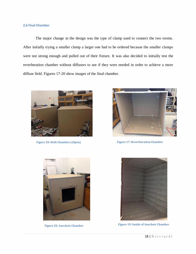
The major change in the design was the type of clamp used to connect the two rooms.
After initially trying a smaller clamp a larger one had to be ordered because the smaller clamps
were not strong enough and pulled out of their fixture. It was also decided to initially test the
reverberation chamber without diffusers to see if they were needed in order to achieve a more
diffuse field. Figures 17-20 show images of the final chamber.
Figure 18: Both Chambers (Open) Figure 17: Reverberation Chamber
Figure 19: Inside of Anechoic Chamber Figure 20: Anechoic Chamber
19 | R i c c i a r d i
Chapter 3: Theoretical Considerations
3.1 Direct and Diffuse Field Theory
As stated in Section 1.1, every sound field has some contributions from the direct field
and diffuse field. The objective for this split chamber design is to have a chamber with an
entirely diffuse field and a chamber with an entirely direct field. However, due to sizing
constraints, this design will not be able to achieve these perfect field conditions.
In a diffuse field the sound pressure is the same at every position in the far field; far field
assumptions excludes positions close to the walls and close to the source (defined as one major
dimension from the source). This assumes that all the boundary conditions are ridged, i.e.
velocity release surface; and that there is no absorption in the room. Therefore if a sound source
exists within the room no energy will ever be dissipated and the energy density in the room
will continue to rise and approach an infinite number of modes. This phenomenon is known as
the “cocktail party effect”. [6] The analogy is to a room of individuals that continue to speak
louder which causes other to speak louder; eventually speech is entirely intelligible and the
sound pressure in the room is so high no one can understand each other. Also, this room would
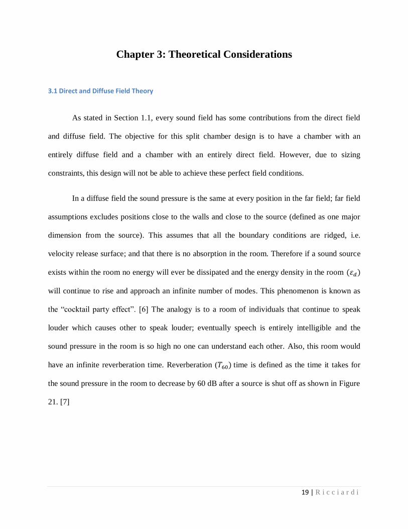
have an infinite reverberation time. Reverberation ( time is defined as the time it takes for
the sound pressure in the room to decrease by 60 dB after a source is shut off as shown in Figure
21. [7]
20 | R i c c i a r d i
Figure 21: Definition of Reverberation Time
However, it is not possible to have such a phenomenon occur. This effect could only occur in a
perfect vacuum since air has absorptive properties; since sound needs a medium in order to
propagate it is not possible to observe this phenomenon. A well-built reverberation chamber will
have reverberation times upwards of 8 seconds [12]. It is often not possible to observe a 60 dB
reduction in the room so reverberation time can be calculated in other manors, described later, or
can be defined for another increment of dB reduction i.e. .
Direct field theory is quite opposite to diffuse field theory; in a perfect direct field
reverberation time would be 0 seconds. In a direct field there are absolutely no reflections from
the boundaries. To understand this concept it is helpful to understand the concept of acoustical
impedance. Specific acoustical impedance is given by Equation 2, where p is the sound pressure
and u is the particle velocity. For anechoic termination at boundary conditions specific
impedance of the boundary (frequency dependent) must equal the impedance in air time the
particle velocity, shown by Equation 3.
( 2 )
( 3 )
21 | R i c c i a r d i
The pressure distribution in a direct field is not uniform; it is related by the inverse square
law as shown in Equation 4 (not valid near the source). As a result of this distribution a doubling
of distance from the source will result in -6 dB change in sound pressure.
[dB]
Both direct and diffuse field theories assume that there is no outside noise leaking into
the room. They also assume a simple lumped theory approach applied to room acoustics.
3.2 Room Modes
The previous section assumed a simple lumped approach; however, there are two more
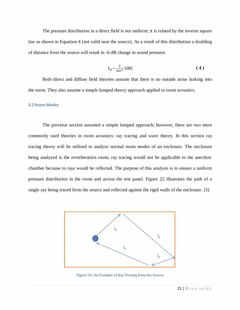
commonly used theories in room acoustics: ray tracing and wave theory. In this section ray
tracing theory will be utilized to analyze normal room modes of an enclosure. The enclosure
being analyzed is the reverberation room; ray tracing would not be applicable to the anechoic
chamber because to rays would be reflected. The purpose of this analysis is to ensure a uniform
pressure distribution in the room and across the test panel. Figure 22 illustrates the path of a
single ray being traced from the source and reflected against the rigid walls of the enclosure. [5]
Figure 22: An Example of Ray Tracing from the Source
( 4 )
22 | R i c c i a r d i
If the total length traveled by a ray is an integer multiple then a normal mode frequency is
reached, shown by Equations 5 and 6. Equation 7 gives us the frequency in Hz of this mode for a
2D case. [5]
[m]
[m]
[Hz]
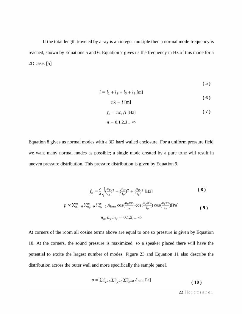
Equation 8 gives us normal modes with a 3D hard walled enclosure. For a uniform pressure field
we want many normal modes as possible; a single mode created by a pure tone will result in
uneven pressure distribution. This pressure distribution is given by Equation 9.
√
[Hz]
∑ ∑ ∑
[Pa]
At corners of the room all cosine terms above are equal to one so pressure is given by Equation
10. At the corners, the sound pressure is maximized, so a speaker placed there will have the
potential to excite the largest number of modes. Figure 23 and Equation 11 also describe the
distribution across the outer wall and more specifically the sample panel.
∑ ∑ ∑
Pa]
( 5 )
( 6 )
( 7 )
( 8 )
( 9 )
( 10 )
23 | R i c c i a r d i
Figure 23: Schematic of Outer Wall With Panel
[Pa]
For purposes of designing this chamber we are mostly concerned with achieve a large number of
modes. Equations 12 and 13 give us a relation for the number of modes N in a given room.
Equation 12 is for narrow band results and Equation 13 is applicable to band widths; where f is
the center frequency and are the major dimensions of the room.
( )
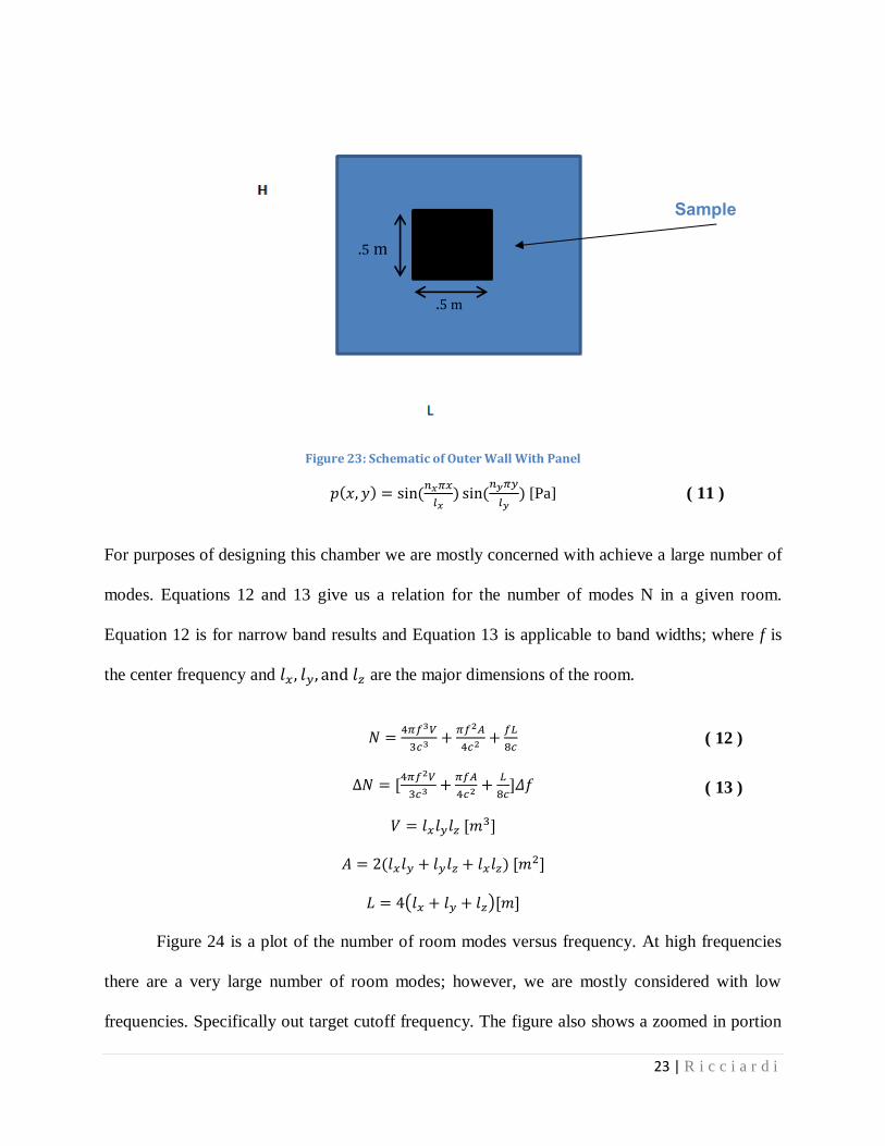
Figure 24 is a plot of the number of room modes versus frequency. At high frequencies
there are a very large number of room modes; however, we are mostly considered with low
frequencies. Specifically out target cutoff frequency. The figure also shows a zoomed in portion
( 12 )
( 13 )
( 11 )
Sample
.5 m
.5 m
24 | R i c c i a r d i
of the plot at the cutoff frequency. At 500 Hz (target cutoff) there are only 40 room modes. This
could cause an issue for uniform pressure distribution at low frequencies. This theory will be
explored experimentally in a later section.
3.3 Surface Interaction (Absorption)
Recall from Figure 1 that when incident sound comes in contact with a surface some of
that sound is reflected back, some is transmitted, and some is absorbed. This section is
considered with the sound that is absorbed and how α is determined.
200 400 600 800 1000 1200 1400
-1
0
1
2
3
4
5
x 104
X: 502
Y: 41.05
Frequency (Hz)
Num
ber
of
Modes
0 1000 2000 3000 4000 5000 6000 7000 8000 9000 100000
0.2
0.4
0.6
0.8
1
1.2
1.4
1.6
1.8
2x 10
5 Number of Room Modes at Given Frequency
Frequency (Hz)
Num
ber
of
Modes
Figure 24: Normal Room Modes
25 | R i c c i a r d i
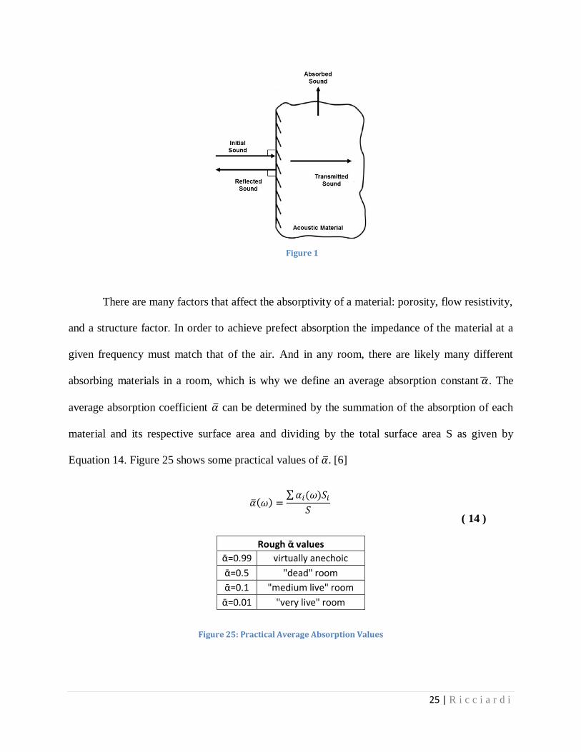
There are many factors that affect the absorptivity of a material: porosity, flow resistivity,
and a structure factor. In order to achieve prefect absorption the impedance of the material at a
given frequency must match that of the air. And in any room, there are likely many different
absorbing materials in a room, which is why we define an average absorption constant . The
average absorption coefficient can be determined by the summation of the absorption of each
material and its respective surface area and dividing by the total surface area S as given by
Equation 14. Figure 25 shows some practical values of [6]
∑
Rough ᾱ values
ᾱ=0.99 virtually anechoic
ᾱ=0.5 "dead" room
ᾱ=0.1 "medium live" room
ᾱ=0.01 "very live" room
Figure 25: Practical Average Absorption Values
Figure 1
( 14 )
26 | R i c c i a r d i
We also define a room constant R as the total absorption power; the effective surface area in the
room with perfect absorption.
Many publications define R defiantly as shown in Equation 16. This equation is generally used
for realistic rooms and for diffuse fields whereas Equation 15 would be more applicable to direct
fields. This value is defined as R’ and is generally used by architects and structural engineers.
This R value can also be experimentally determined by using Equation 17. This R value can then
be used to calculate from Equation 15 or 16. This procedure will be utilized later for
experimental evaluation both chambers.
[dB]
Where is a measured value, is of a known power source,
is the contribution from
direct field, =1 for spherical radiation; 2 for hemispherical radiation, and
is the contribution
from the diffuse field. R can also be used to find reverberation time from Equation 18 and then
the cutoff frequency using Equation 19.
[s]
√
[Hz]
( 15 )
( 16 )
( 17 )
( 18 )
( 19 )
27 | R i c c i a r d i
3.4 Surface Interaction (Transmission)
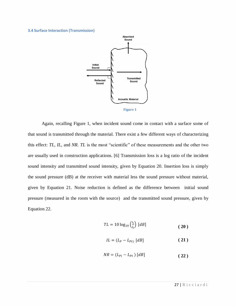
Again, recalling Figure 1, when incident sound come in contact with a surface some of
that sound is transmitted through the material. There exist a few different ways of characterizing
this effect: TL, IL, and NR. TL is the most “scientific” of these measurements and the other two
are usually used in construction applications. [6] Transmission loss is a log ratio of the incident
sound intensity and transmitted sound intensity, given by Equation 20. Insertion loss is simply
the sound pressure (dB) at the receiver with material less the sound pressure without material,
given by Equation 21. Noise reduction is defined as the difference between initial sound
pressure (measured in the room with the source) and the transmitted sound pressure, given by
Equation 22.
(
)
Figure 1
( 21 )
( 22 )
( 20 )
28 | R i c c i a r d i
3.5 Evaluation Criterion
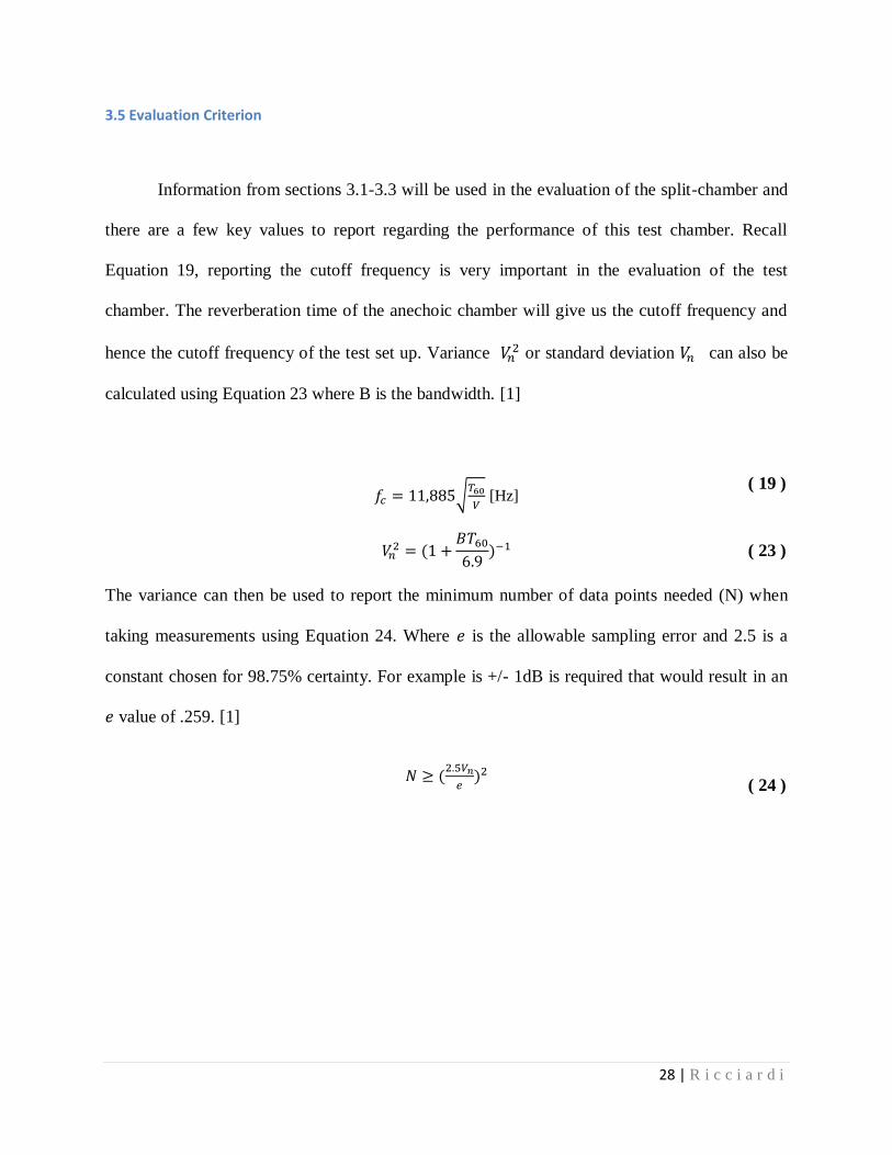
Information from sections 3.1-3.3 will be used in the evaluation of the split-chamber and
there are a few key values to report regarding the performance of this test chamber. Recall
Equation 19, reporting the cutoff frequency is very important in the evaluation of the test
chamber. The reverberation time of the anechoic chamber will give us the cutoff frequency and
hence the cutoff frequency of the test set up. Variance or standard deviation can also be
calculated using Equation 23 where B is the bandwidth. [1]
√
[Hz]
The variance can then be used to report the minimum number of data points needed (N) when
taking measurements using Equation 24. Where is the allowable sampling error and 2.5 is a
constant chosen for 98.75% certainty. For example is +/- 1dB is required that would result in an
value of .259. [1]
( 19 )
( 23 )
( 24 )
29 | R i c c i a r d i
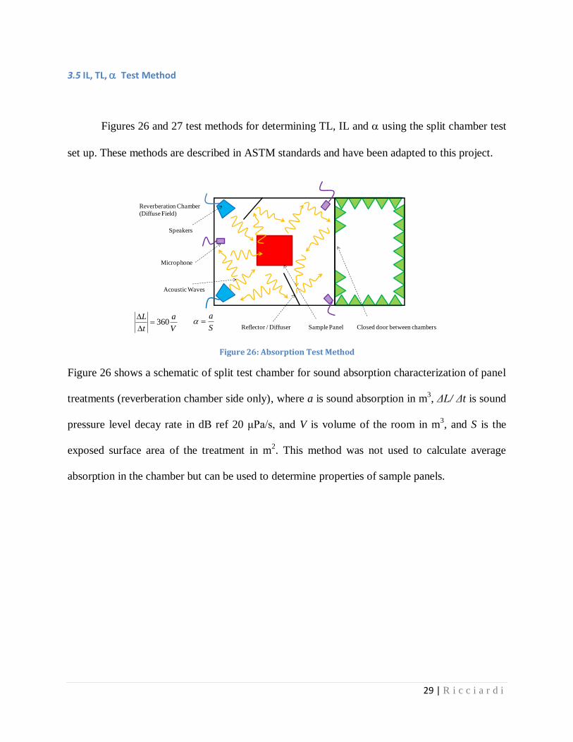
3.5 IL, TL, Test Method
Figures 26 and 27 test methods for determining TL, IL and using the split chamber test
set up. These methods are described in ASTM standards and have been adapted to this project.
Figure 26: Absorption Test Method
Figure 26 shows a schematic of split test chamber for sound absorption characterization of panel
treatments (reverberation chamber side only), where a is sound absorption in m3, ΔL/ Δt is sound
pressure level decay rate in dB ref 20 μPa/s, and V is volume of the room in m3, and S is the
exposed surface area of the treatment in m2. This method was not used to calculate average
absorption in the chamber but can be used to determine properties of sample panels.
Reverberation Chamber
(Diffuse Field)
Reflector / Diffuser
Speakers
Sample Panel
Acoustic Waves
Microphone
Closed door between chambersV
a
t
L360
a
S
30 | R i c c i a r d i
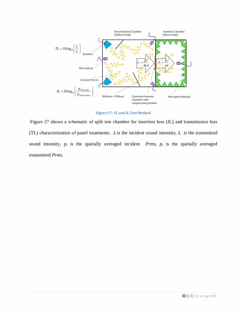
Figure 27: TL and IL Test Method
Figure 27 shows a schematic of split test chamber for insertion loss (IL) and transmission loss
(TL) characterization of panel treatments. Ii is the incident sound intensity, It is the transmitted
sound intensity, pi is the spatially averaged incident Prms, pt is the spatially averaged
transmitted Prms.
Reverberation Chamber
(Diffuse Field)
Anechoic Chamber
(Direct Field)
Reflector / Diffuser Absorptive Material
Speakers
Open door between
chambers with
sample panel partition
Acoustic Waves
Microphone
2
tt
pI
c
2
4
ii
pI
c
1010log i
t
ITL
I
with panel
10
without panel
20logp
ILp
31 | R i c c i a r d i
Chapter 4: Experimental Evaluation
4.1 Testing Set-Ups
A variety of test set-ups were used in the evaluation of this design. In each test set up
background noise data was collected to ensure results were more than 10 dB above background
noise to avoid any need for background correction. Also, all sound pressure data collected was
rms data given by Equations 25 and 26.
∫
=Sound Pressure Data Collected
[dB]
The first set up was using a known power source to measure for
both chambers and to determine the cutoff frequency of the anechoic chamber. The power
source, shown in mounted in Figure 28, was manufactured by ILG Industries. It is essentially a
fan than produces a known power level at given frequencies. [9] The mounting shown in Figure
28 is assumed to hemi-spherical (defined by equation 17).
( 25 )
( 26 )
32 | R i c c i a r d i
Figure 28: Mounted Power Source
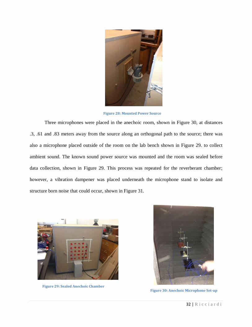
Three microphones were placed in the anechoic room, shown in Figure 30, at distances
.3, .61 and .83 meters away from the source along an orthogonal path to the source; there was
also a microphone placed outside of the room on the lab bench shown in Figure 29. to collect
ambient sound. The known sound power source was mounted and the room was sealed before
data collection, shown in Figure 29. This process was repeated for the reverberant chamber;
however, a vibration dampener was placed underneath the microphone stand to isolate and
structure born noise that could occur, shown in Figure 31.
Figure 30: Anechoic Microphone Set-up Figure 29: Sealed Anechoic Chamber
33 | R i c c i a r d i
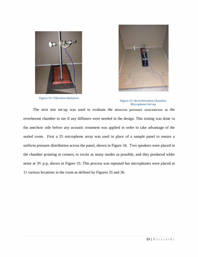
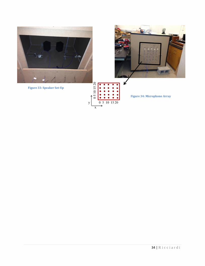
The next test set-up was used to evaluate the uniform pressure distribution in the
reverberant chamber to see if any diffusers were needed in the design. This testing was done in
the anechoic side before any acoustic treatment was applied in order to take advantage of the
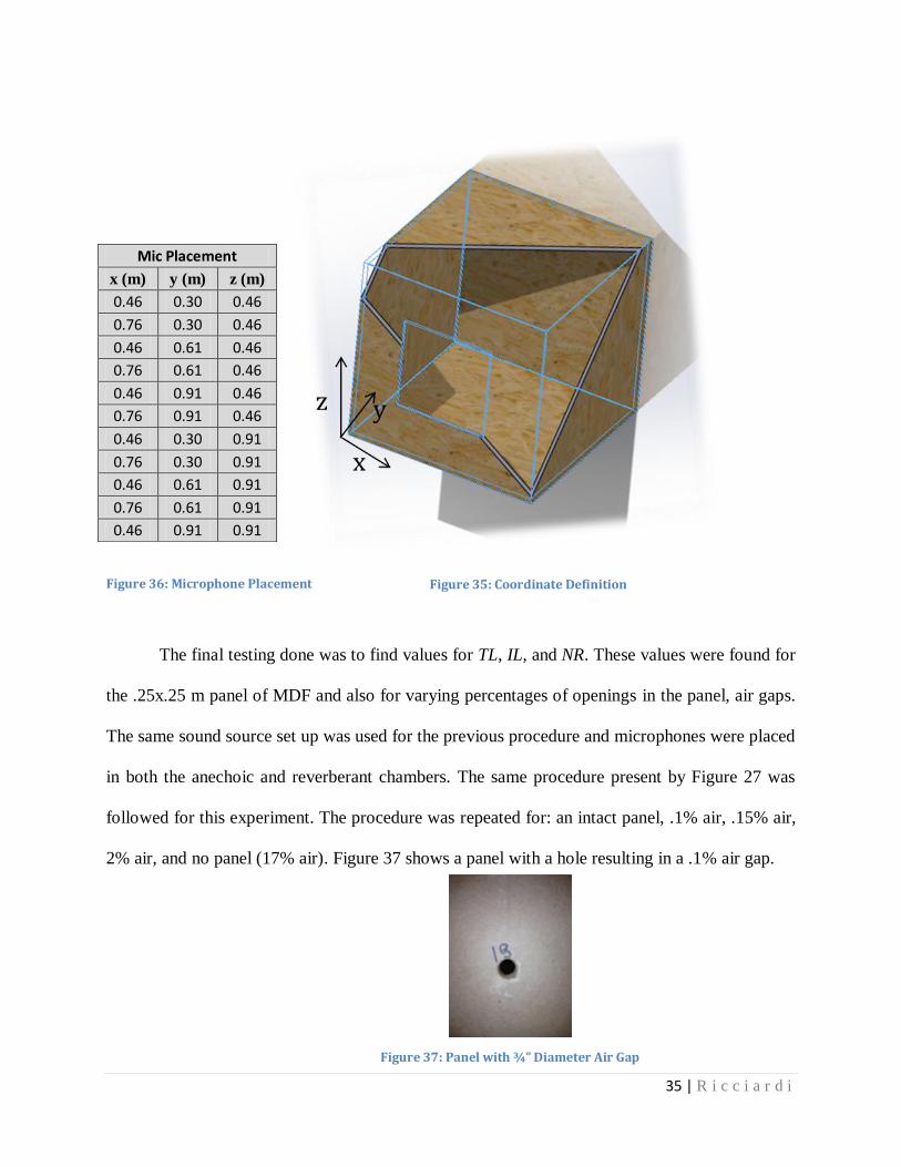
sealed room. First a 25 microphone array was used in place of a sample panel to ensure a
uniform pressure distribution across the panel, shown in Figure 34. Two speakers were placed in
the chamber pointing at corners, to excite as many modes as possible, and they produced white
noise at 3V p-p, shown in Figure 33. This process was repeated but microphones were placed at
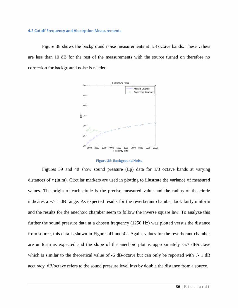
11 various locations in the room as defined by Figures 35 and 36.
Figure 32: Reverberation Chamber Microphone Set-up
Figure 31: Vibration Idolaters
34 | R i c c i a r d i
Figure 34: Microphone Array
Figure 33: Speaker Set-Up
35 | R i c c i a r d i
Figure 36: Microphone Placement
The final testing done was to find values for TL, IL, and NR. These values were found for
the .25x.25 m panel of MDF and also for varying percentages of openings in the panel, air gaps.
The same sound source set up was used for the previous procedure and microphones were placed
in both the anechoic and reverberant chambers. The same procedure present by Figure 27 was
followed for this experiment. The procedure was repeated for: an intact panel, .1% air, .15% air,
2% air, and no panel (17% air). Figure 37 shows a panel with a hole resulting in a .1% air gap.
Mic Placement
x (m) y (m) z (m)
0.46 0.30 0.46
0.76 0.30 0.46
0.46 0.61 0.46
0.76 0.61 0.46
0.46 0.91 0.46
0.76 0.91 0.46
0.46 0.30 0.91
0.76 0.30 0.91
0.46 0.61 0.91
0.76 0.61 0.91
0.46 0.91 0.91
Figure 35: Coordinate Definition
Figure 37: Panel with ¾” Diameter Air Gap
36 | R i c c i a r d i
4.2 Cutoff Frequency and Absorption Measurements
Figure 38 shows the background noise measurements at 1/3 octave bands. These values
are less than 10 dB for the rest of the measurements with the source turned on therefore no
correction for background noise is needed.
Figure 38: Background Noise
Figures 39 and 40 show sound pressure (Lp) data for 1/3 octave bands at varying
distances of r (in m). Circular markers are used in plotting to illustrate the variance of measured
values. The origin of each circle is the precise measured value and the radius of the circle
indicates a +/- 1 dB range. As expected results for the reverberant chamber look fairly uniform
and the results for the anechoic chamber seem to follow the inverse square law. To analyze this
further the sound pressure data at a chosen frequency (1250 Hz) was plotted versus the distance
from source, this data is shown in Figures 41 and 42. Again, values for the reverberant chamber
are uniform as expected and the slope of the anechoic plot is approximately -5.7 dB/octave
which is similar to the theoretical value of -6 dB/octave but can only be reported with+/- 1 dB
accuracy. dB/octave refers to the sound pressure level loss by double the distance from a source.
1000 2000 3000 4000 5000 6000 7000 8000 9000 1000020
25
30
35
40
45
50Background Noise
Frequency (Hz)
(dB
)
Anehoic Chamber
Reverberant Chamber
37 | R i c c i a r d i
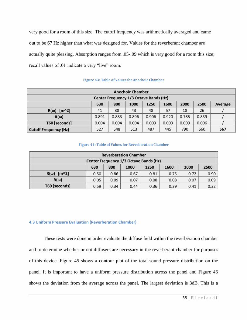
This test set up was also used to find value for for each room at 1/3
octave bands. It was chosen to report from 630 Hz to 2500 Hz because the ASTM standards
report 1/3 octave band data similarly. Figures 43 and 44 show this data. Values for should
be as close to 1 as possible and values for this chamber range from .78 to .92; these values are
0.4 0.5 0.6 0.7 0.8 0.9 160
65
70
75
80
85
90
Lp (
dB
) at
f=1250 H
z (
1/3
octa
ve b
and)
Distance From Source (m)
Sound Pressure vs Distance for 1/3 Octave Band Center Frequency=1250Hz
Anechoic Chamber Data
Figure 39: 1/3 Octave Band Spectrum for Reverberant Chamber at Varying Distances r
Figure 40: 1/3 Octave Band Spectrum for Anechoic Chamber at Varying Distances r
Slope approx. -5.7 dB/octave
Figure 42: Reverberant Lp vs Distance From Source Figure 41: Anechoic Lp vs Distance From Source
0.4 0.5 0.6 0.7 0.8 0.9 160
65
70
75
80
85
90
Lp (
dB
) at
f=1250 H
z (
1/3
octa
ve b
and)
Distance From Source (m)
Sound Pressure vs Distance for 1/3 Octave Band Center Frequency=1250Hz
Reverberant Chamber Data
1000 2000 3000 4000 5000 6000 7000 8000 9000 1000030
35
40
45
50
55
60
65
70
75
80Anechoic Sound Pressure at Varying Distances
Frequency (Hz)
Lp (
dB
)
r=.3m
r=.6m
r=.83m
Outside of Chamber
1000 2000 3000 4000 5000 6000 7000 8000 9000 1000030
40
50
60
70
80
90Reverberant Sound Pressure at Varying Distances
Frequency (Hz)
Lp (
dB
)
r=.3m
r=.6m
r=.83m
Outside of Chamber
38 | R i c c i a r d i
very good for a room of this size. The cutoff frequency was arithmetically averaged and came
out to be 67 Hz higher than what was designed for. Values for the reverberant chamber are
actually quite pleasing. Absorption ranges from .05-.09 which is very good for a room this size;
recall values of .01 indicate a very “live” room.
Figure 43: Table of Values for Anechoic Chamber
Figure 44: Table of Values for Reverberation Chamber
4.3 Uniform Pressure Evaluation (Reverberation Chamber)
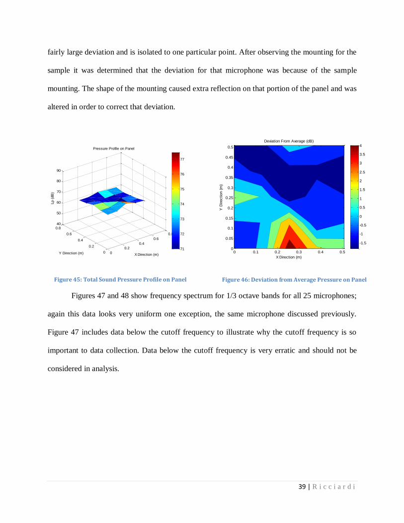
These tests were done in order evaluate the diffuse field within the reverberation chamber
and to determine whether or not diffusers are necessary in the reverberant chamber for purposes
of this device. Figure 45 shows a contour plot of the total sound pressure distribution on the
panel. It is important to have a uniform pressure distribution across the panel and Figure 46
shows the deviation from the average across the panel. The largest deviation is 3dB. This is a
Anechoic Chamber
Center Frequency 1/3 Octave Bands (Hz)
630 800 1000 1250 1600 2000 2500 Average
R(ω) [m^2] 41 38 43 48 57 18 26 /
ᾱ(ω) 0.891 0.883 0.896 0.906 0.920 0.785 0.839 /
T60 [seconds] 0.004 0.004 0.004 0.003 0.003 0.009 0.006 /
Cutoff Frequency (Hz) 527 548 513 487 445 790 660 567
Reverberation Chamber
Center Frequency 1/3 Octave Bands (Hz)
630 800 1000 1250 1600 2000 2500
R(ω) [m^2] 0.50 0.86 0.67 0.81 0.75 0.72 0.90
ᾱ(ω) 0.05 0.09 0.07 0.08 0.08 0.07 0.09
T60 [seconds] 0.59 0.34 0.44 0.36 0.39 0.41 0.32
39 | R i c c i a r d i
fairly large deviation and is isolated to one particular point. After observing the mounting for the
sample it was determined that the deviation for that microphone was because of the sample
mounting. The shape of the mounting caused extra reflection on that portion of the panel and was
altered in order to correct that deviation.
Figures 47 and 48 show frequency spectrum for 1/3 octave bands for all 25 microphones;
again this data looks very uniform one exception, the same microphone discussed previously.
Figure 47 includes data below the cutoff frequency to illustrate why the cutoff frequency is so
important to data collection. Data below the cutoff frequency is very erratic and should not be
considered in analysis.
Figure 45: Total Sound Pressure Profile on Panel Figure 46: Deviation from Average Pressure on Panel
X Direction (m)
Y D
irection (
m)
Deviation From Average (dB)
0 0.1 0.2 0.3 0.4 0.50
0.05
0.1
0.15
0.2
0.25
0.3
0.35
0.4
0.45
0.5
-1.5
-1
-0.5
0
0.5
1
1.5
2
2.5
3
3.5
4
0
0.2
0.4
0.6
0.8
0
0.2
0.4
0.6
0.840
50
60
70
80
90
X Direction (m)
Pressure Profile on Panel
Y Direction (m)
Lp (
dB
)
71
72
73
74
75
76
77
40 | R i c c i a r d i
Similar plots are shown by Figures 49 and 50 for data taken at various points in the room.
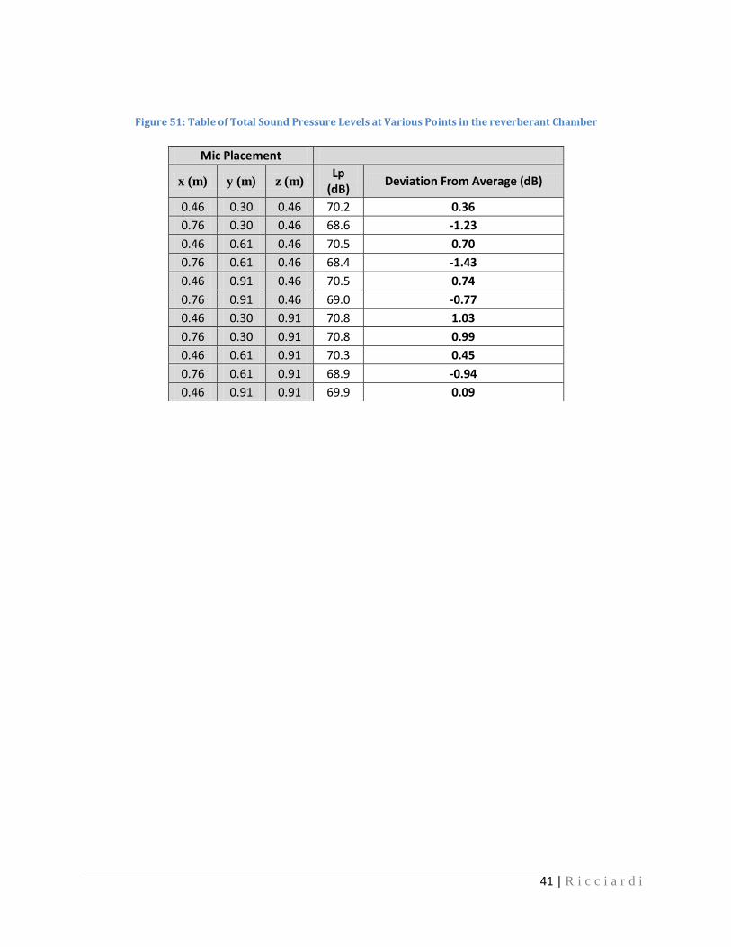
Again Figure 49 illustrates the data near the cutoff frequency and Figure 50 shows very similar
distributions for various points in the room. Figure 51 shows a table of the total sound pressures
found at various points in the room. Deviation of +/-1 dB can be dismissed as insignificant
deviation; the maximum value of deviation in this field is 1.43 dB which is very low. [1]
Therefore, it can be assumed that this is a diffuse field for purposes of this project and no
diffusers are needed for this frequency range.
-200 0 200 400 600 800 1000 1200
35
40
45
50
55
60
65
Frequency (Hz)
Lp (
dB
)
25 Mic Array with White Noise (1/3 Octave Band)
0.2 0.4 0.6 0.8 1 1.2 1.4 1.6 1.8 2
x 104
40
50
60
70
80
90
100
Frequency (Hz)
Lp (
dB
)
25 Mic Array with White Noise (1/3 Octave Band)
0 500 1000 1500 2000 2500 3000 3500 4000 4500
30
35
40
45
50
55
60
65
Frequency (Hz)
Lp (
dB
)
1/3 Octave Band Data at Various Points in Room
2000 4000 6000 8000 10000 12000 14000 16000 18000
45
50
55
60
65
70
75
80
85
Frequency (Hz)
Lp (
dB
)
1/3 Octave Band Data at Various Points in Room
Figure 47: 1/3 Octave Band Frequency Spectrum for all 25 Microphones
Figure 48: 25 Microphone Array 1/3 Octave Band Frequency Spectrum Near Cutoff Frequency
Figure 49: 1/3 Octave Band Frequency Spectrum Near Cutoff Frequency for Various Points in the Room
Figure 50: 1/3 Octave Band Frequency Spectrum for Various Points in the Room
41 | R i c c i a r d i
Figure 51: Table of Total Sound Pressure Levels at Various Points in the reverberant Chamber
Mic Placement
x (m) y (m) z (m) Lp
(dB) Deviation From Average (dB)
0.46 0.30 0.46 70.2 0.36
0.76 0.30 0.46 68.6 -1.23
0.46 0.61 0.46 70.5 0.70
0.76 0.61 0.46 68.4 -1.43
0.46 0.91 0.46 70.5 0.74
0.76 0.91 0.46 69.0 -0.77
0.46 0.30 0.91 70.8 1.03
0.76 0.30 0.91 70.8 0.99
0.46 0.61 0.91 70.3 0.45
0.76 0.61 0.91 68.9 -0.94
0.46 0.91 0.91 69.9 0.09
42 | R i c c i a r d i
4.4 Transmission Loss Measurements
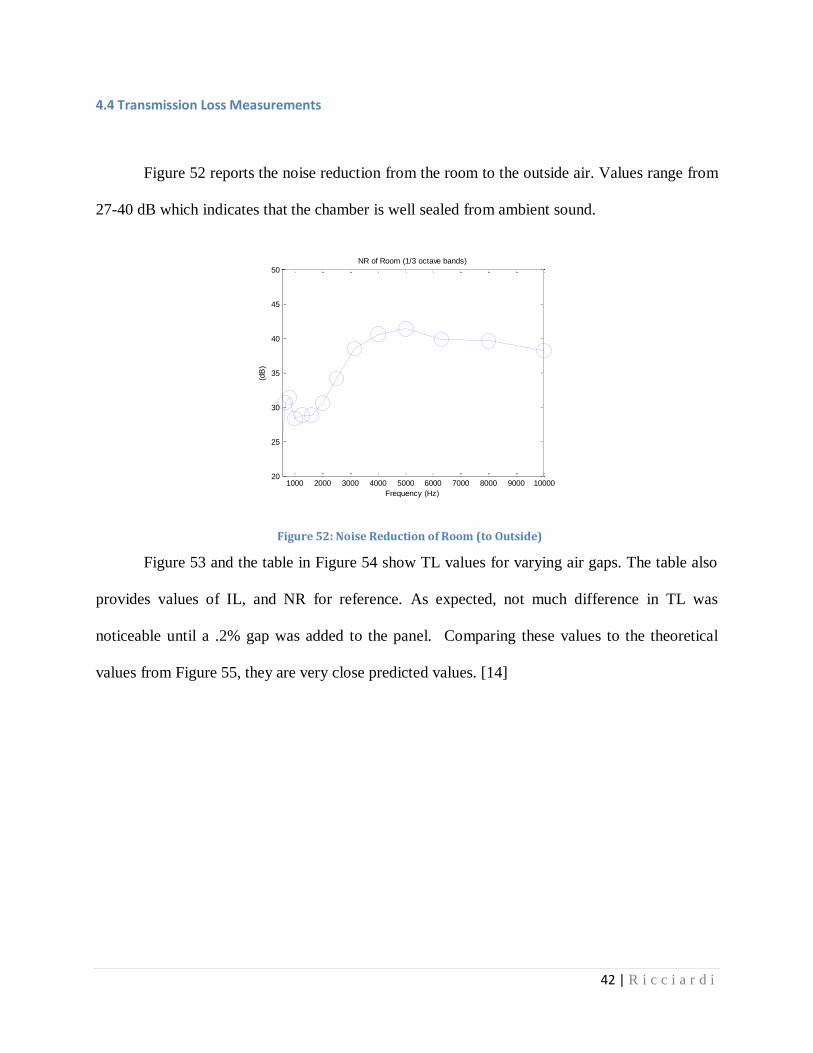
Figure 52 reports the noise reduction from the room to the outside air. Values range from
27-40 dB which indicates that the chamber is well sealed from ambient sound.
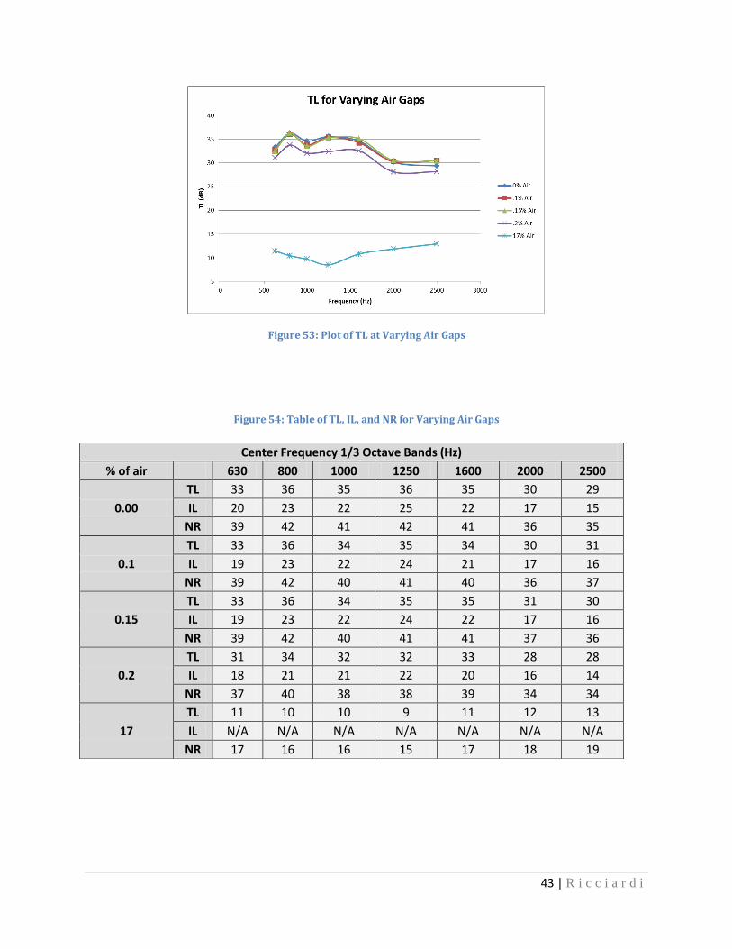
Figure 53 and the table in Figure 54 show TL values for varying air gaps. The table also
provides values of IL, and NR for reference. As expected, not much difference in TL was
noticeable until a .2% gap was added to the panel. Comparing these values to the theoretical
values from Figure 55, they are very close predicted values. [14]
1000 2000 3000 4000 5000 6000 7000 8000 9000 1000020
25
30
35
40
45
50NR of Room (1/3 octave bands)
Frequency (Hz)
(dB
)
Figure 52: Noise Reduction of Room (to Outside)
43 | R i c c i a r d i
Figure 53: Plot of TL at Varying Air Gaps
Figure 54: Table of TL, IL, and NR for Varying Air Gaps
Center Frequency 1/3 Octave Bands (Hz)
% of air 630 800 1000 1250 1600 2000 2500
0.00
TL 33 36 35 36 35 30 29
IL 20 23 22 25 22 17 15
NR 39 42 41 42 41 36 35
0.1
TL 33 36 34 35 34 30 31
IL 19 23 22 24 21 17 16
NR 39 42 40 41 40 36 37
0.15
TL 33 36 34 35 35 31 30
IL 19 23 22 24 22 17 16
NR 39 42 40 41 41 37 36
0.2
TL 31 34 32 32 33 28 28
IL 18 21 21 22 20 16 14
NR 37 40 38 38 39 34 34
17
TL 11 10 10 9 11 12 13
IL N/A N/A N/A N/A N/A N/A N/A
NR 17 16 16 15 17 18 19
44 | R i c c i a r d i
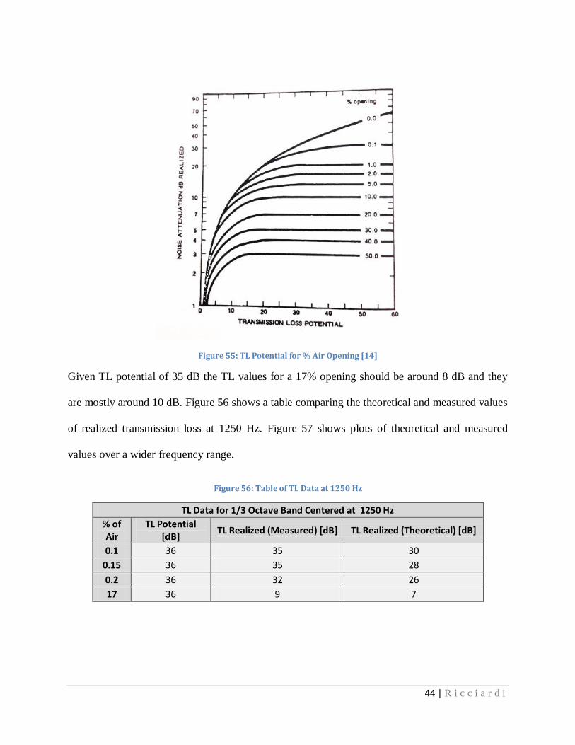
Figure 55: TL Potential for % Air Opening [14]
Given TL potential of 35 dB the TL values for a 17% opening should be around 8 dB and they
are mostly around 10 dB. Figure 56 shows a table comparing the theoretical and measured values
of realized transmission loss at 1250 Hz. Figure 57 shows plots of theoretical and measured
values over a wider frequency range.
Figure 56: Table of TL Data at 1250 Hz
TL Data for 1/3 Octave Band Centered at 1250 Hz
% of Air
TL Potential [dB]
TL Realized (Measured) [dB] TL Realized (Theoretical) [dB]
0.1 36 35 30
0.15 36 35 28
0.2 36 32 26
17 36 9 7

45 | R i c c i a r d i
Figure 57: Comparing Theoretical and Experimental TL
5
10
15
20
25
30
35
40
0 500 1000 1500 2000 2500 3000
TL
(d
B)
Frequency (Hz)
TL for Varying Air Gaps (Theory and Experimental)
TL Potential
.2% Air (Measured)
17% Air (Measured)
.2% (Theory)
17% (Theory)
46 | R i c c i a r d i
Chapter 5: Conclusions
5.1 Conclusion
The main objective of this project was to develop a test to characterize random incidence
properties of acoustic materials. By reviewing ASTM standards it was determined that a split
chamber design would be the best solution for this project. Given sizing and budgetary
constraints at target cutoff frequency of 500 Hz was chosen. The design process included several
iterations but the final chamber was very similar to the final design. This chamber was built to be
within the sizing constraints and under budget. Evaluation of this chamber yielded a cutoff
frequency of approximately 570 Hz which is above the target, however it is very reasonable
considering the constraints and the purposes of this chamber. The theoretical calculations
consisted of both field theory and surface interaction. A great deal of time was spent
characterizing the field within each room; this is a valuable concept to understand and to have
experience with considering that the purpose of this chamber is to characterize materials that
treat such rooms of varying contributions from the direct and diffuse fields.
Values of were determined for both anechoic and reverberant rooms.
The anechoic chamber yielded values ranging from .78 to .9 and reverberation times
ranging from .003 seconds to .008 seconds. These values are quite reasonable considering that
the anechoic chamber in this design could nearly be considered hemi-anechoic because of the
large amount of surface area not treated (the sample size). The slope for sound pressures at
varying distances from the source was found to be -5.7 dB/octave which is very close to the -6
dB/octave theoretical value. The reverberant chamber yielded values ranging from .05 to
.09 and reverberation times from .32 seconds to .59 seconds. This values fall within reasonably
47 | R i c c i a r d i
expected values. When total sound pressures were analyzed in a 25 microphone array on the
panel there was hardly any deviation except for one point; this deviation was a result of the
mounting. When the diffuse field was evaluated by taking total sound pressure measurements it
was determined that the pressure in the room was sufficiently uniform and no diffusers were
needed.
TL data was collected for the room itself and it was determined that the room was
well sealed and there is no need for further insulation. When TL data was collected for varying
air gaps measured results yielded values very close to theoretical. With a 17% opening there was
a TL of 10 dB realized when theoretical values were near 7 dB. The main objective of the
project was completed; there is now a test chamber and a test method for determining
values for acoustic materials. This chamber was never intended to meet the ASTM standards but
will serve as a valuable tool for the Acoustic and Dynamics Laboratory and for future
educational purposes in Mechanical Engineering coursework. Those classes include ME 8260
(Advanced Acoustics) and the Auto NVH sequence.
5.2 Sources of Error
Acoustic experimental measurements measure very small pressure perturbations from
equilibrium. It is extremely difficult to report these measurements within a high degree of
accuracy, thus there are several sources within any acoustic testing set-up that might cause error.
Faulty equipment; microphones, cable, data acquisition systems, etc. can cause significant error
if not properly calibrated. However, most measurements for this project were relative
measurements and microphones had been previously calibrated. A simple yet significant source
of error would be distance measurements. Distance measurements such as room size and distance
48 | R i c c i a r d i
from the source were taken with a standard tape measure and can only provide accuracy to the
nearest 5 mm. The biggest source of error from these experiments would be structural borne
noise. Sound sources often have both airborne and structural borne noise components and all
measurements and calculations assumed only airborne noise. Structural borne noise would come
from the sound source (either known power source or the speakers) exciting the enclosure walls
to which it is attached. This structural borne noise would increase all of the sound pressure
values; which is less important for relative measurements but would result in higher values for
absorption. Ways to improve this error would be to add more dampening to the structure; this
could be done by applying mass loaded vinyl (MLV) to the sample mounting brackets and to the
mounting for the sound sources. MLV or other vibration absorbers could be added to the outside
of enclosure walls to reduce structure borne vibrations.
5.3 Recommendations for Future work
The design itself turned out just as expected but I would change a few things to increase
the accuracy of the chamber. Firstly, large acoustic wedges should be added to the anechoic
side. The reasoning for buying 6” of acoustic material was because of budgetary constraints. In
order to maximize performance another $500 would be necessary to increase the amount of foam
to 12”. Future work would also include exploring the possibility of using diffusers in the
reverberant chamber. As part of my ME 8260 coursework I will analyze the effects of diffusers
with boundary element software (Coustyx) and compare this with experimental results.
This chamber can be used for the purpose defined in section 3.5; however, this test
chamber can also be altered to serve as an anechoic test chamber. By simply adding a wire grid
to cover the bottom foam wedges, objects could be placed in the room for testing. Also, future
49 | R i c c i a r d i
work might include developing laboratory exercises for the various classes involving acoustics.
This would also involve promoting the use of the chamber.
50 | R i c c i a r d i
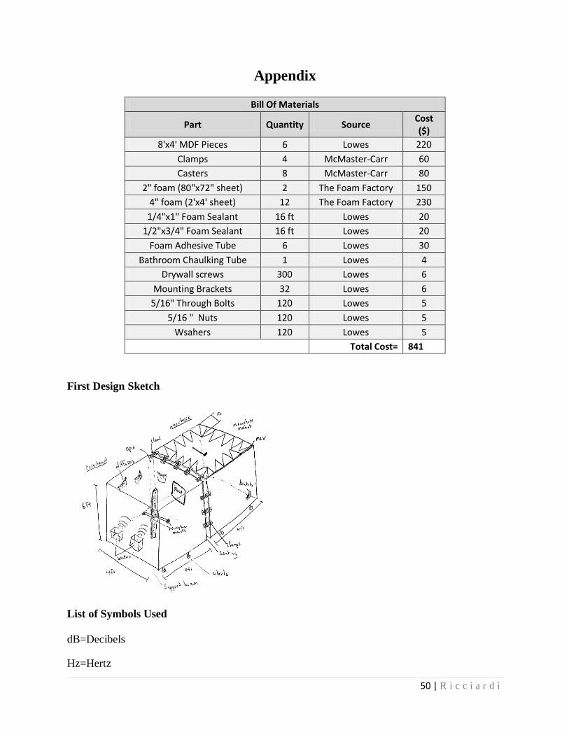
Appendix
Bill Of Materials
Part Quantity Source Cost ($)
8'x4' MDF Pieces 6 Lowes 220
Clamps 4 McMaster-Carr 60
Casters 8 McMaster-Carr 80
2" foam (80"x72" sheet) 2 The Foam Factory 150
4" foam (2'x4' sheet) 12 The Foam Factory 230
1/4"x1" Foam Sealant 16 ft Lowes 20
1/2"x3/4" Foam Sealant 16 ft Lowes 20
Foam Adhesive Tube 6 Lowes 30
Bathroom Chaulking Tube 1 Lowes 4
Drywall screws 300 Lowes 6
Mounting Brackets 32 Lowes 6
5/16" Through Bolts 120 Lowes 5
5/16 " Nuts 120 Lowes 5
Wsahers 120 Lowes 5
Total Cost= 841
First Design Sketch
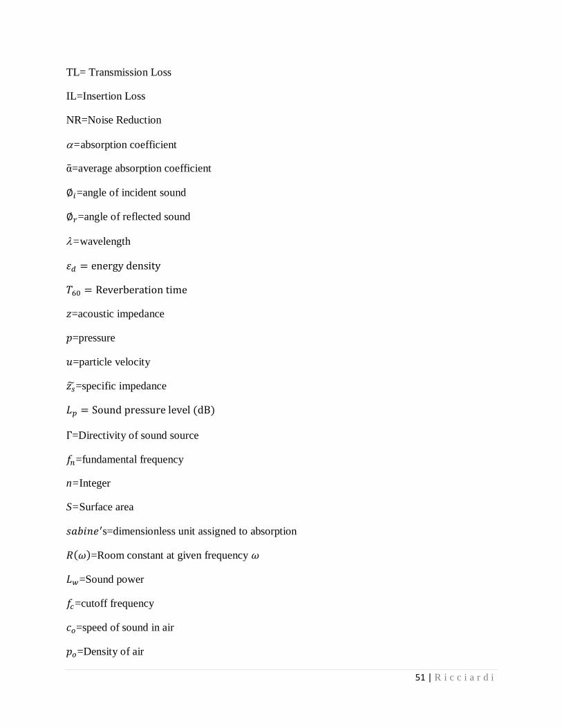
List of Symbols Used
dB=Decibels
Hz=Hertz
51 | R i c c i a r d i
TL= Transmission Loss
IL=Insertion Loss
NR=Noise Reduction
=absorption coefficient
ᾱ=average absorption coefficient
=angle of incident sound
=angle of reflected sound
=wavelength
=acoustic impedance
=pressure
=particle velocity
=specific impedance
=Directivity of sound source
=fundamental frequency
n=Integer
S=Surface area
s=dimensionless unit assigned to absorption
=Room constant at given frequency
=Sound power
=cutoff frequency
=speed of sound in air
=Density of air
52 | R i c c i a r d i
=Incident sound intensity
=Variance
N=number of samples
=Root mean square pressure
References
[1] Lord, Harold W., William S. Gatley, and Harold A. Evensen. Noise Control For Engineers.
Malabar: Krieger, 1980.
[2] ASTM E90, “Standard Test Method for Laboratory Measurement of Airborne Sound
Transmission Loss of Building Partitions and Elements.” ASTM International, West
Conshohocken, PA, 2009.
[3] ASTM C423, “Standard Test Method for Sound Absorption and Sound Absorption
coefficient by the Reverberation Room Method.” ASTM International, West
Conshohocken, PA, 2009.
[4] Everest, Alton F. Master Handbook of Acoustics. Fifth ed. New York: Mc Graw Hill, 2009.
[5] A. Kahraman, “MechEng 5240 Engineering Acoustics” Spring 2013
[6] R. Singh, “ME 8260 Course Notes Advanced Engineering Acoustics” SP 2013 Edition
[7] Bruel &Kjaer, Measurements in Building Acoustic. 1988s
53 | R i c c i a r d i
[8] Pierce, Allan D. Acoustics: An Introduction to Its Physical Principles and Applications. New
Zealand: Mc Graw Hill, 1989..
[9] Reference sound source. Manufacturer: ILG Industries, Inc., 2826 North Pulaki Road,
Chicago, Ill. 60641.
[10] "Acoustic Test Chambers." | ETS-Lindgren. N.p., n.d. Web. 12 Mar. 2013.
[11] ASTM C384, “Standard Test Method for Impedence and Absorption of Acoustic Masterials
by Impedence Tube Method.” ASTM International, West Conshohocken, PA, 2009.
[12] "Performance Testing." Architectural Testing:. N.p., n.d. Web. 12 Mar. 2013
[13] "McMaster-Carr." McMaster-Carr. N.p., n.d. Web. 12 Mar. 2013.
[14] Rao, Mohan D., and Harold A. Evensen. Supplemental Notes to Acoustics and Noise
Control. N.p.: Michigan Tech University, n.d. Print.