Embed Size (px)
Citation preview

Design of a Simulink-Based Control
Workstation for Mobile Wheeled Vehicles with
Variable-Velocity Differential Motor Drives
Kevin Block, Timothy De Pasion, Benjamin Roos, Alexander SchmidtGary Dempsey
Bradley University Electrical and Computer Engineering Department
March 1, 2016
Presentation Outline
•Background•Benjamin Roos•Timothy De Pasion•Alexander Schmidt•Kevin Block•Conclusion
2
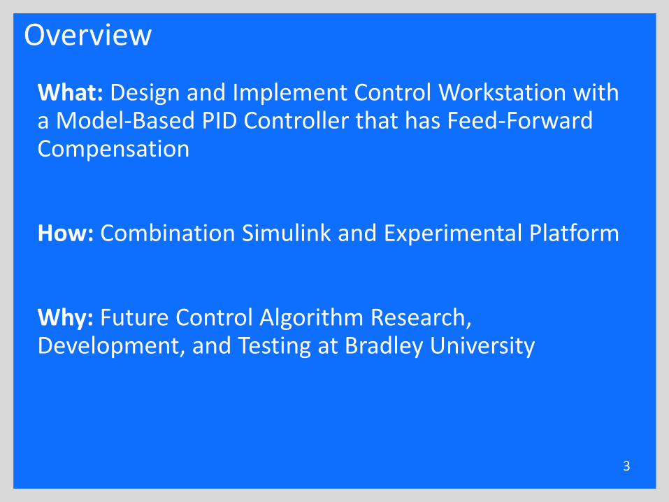
Overview
What: Design and Implement Control Workstation with a Model-Based PID Controller that has Feed-Forward Compensation
How: Combination Simulink and Experimental Platform
Why: Future Control Algorithm Research, Development, and Testing at Bradley University
3
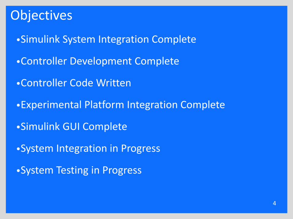
Objectives
•Simulink System Integration Complete
•Controller Development Complete
•Controller Code Written
•Experimental Platform Integration Complete
•Simulink GUI Complete
•System Integration in Progress
•System Testing in Progress
4
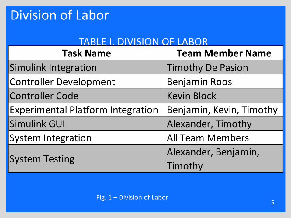
Division of Labor
5
TABLE I. DIVISION OF LABORTask Name Team Member Name
Simulink Integration Timothy De Pasion
Controller Development Benjamin Roos
Controller Code Kevin Block
Experimental Platform Integration Benjamin, Kevin, Timothy
Simulink GUI Alexander, Timothy
System Integration All Team Members
System TestingAlexander, Benjamin,
Timothy
Fig. 1 – Division of Labor

Overview
6Fig. 2 – High Level Block Diagram

Experimental Platform
7
Fig. 3 – Experimental Platform Block Diagram
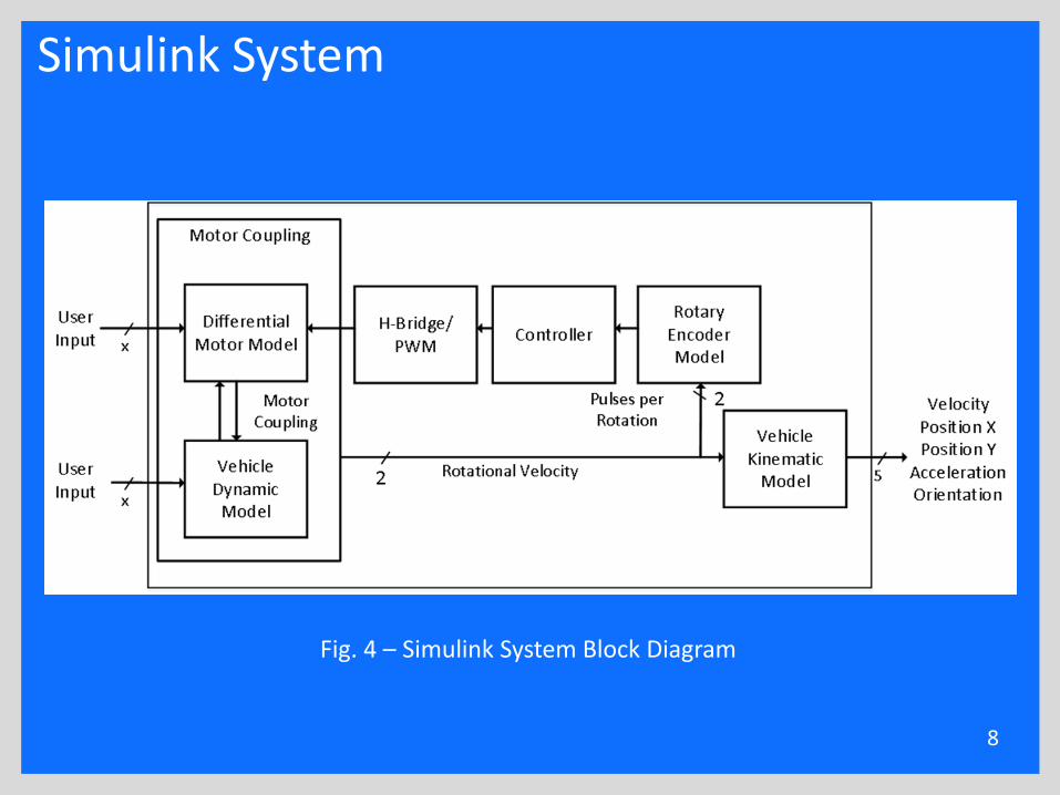
Simulink System
8
Fig. 4 – Simulink System Block Diagram
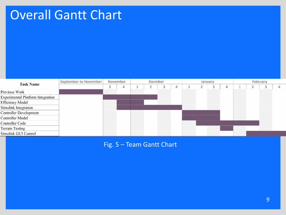
Overall Gantt Chart
9
Fig. 5 – Team Gantt Chart

Presentation Outline
•Background•Benjamin Roos•Timothy De Pasion•Alexander Schmidt•Kevin Block•Conclusion
10
Presentation Outline
•Background•Benjamin Roos
•Controller Development – PI Feedback Controller•Controller Specification Verification•Current Source and Dynamic Model Matching
•Timothy De Pasion•Alexander Schmidt•Kevin Block•Conclusion
11
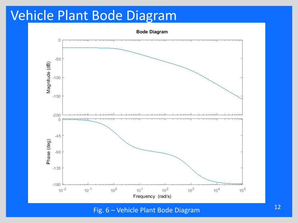
Vehicle Plant Bode Diagram
12Fig. 6 – Vehicle Plant Bode Diagram
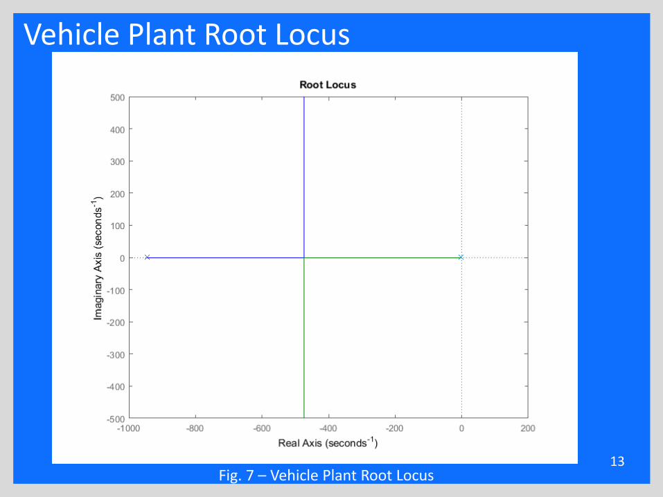
Vehicle Plant Root Locus
13Fig. 7 – Vehicle Plant Root Locus
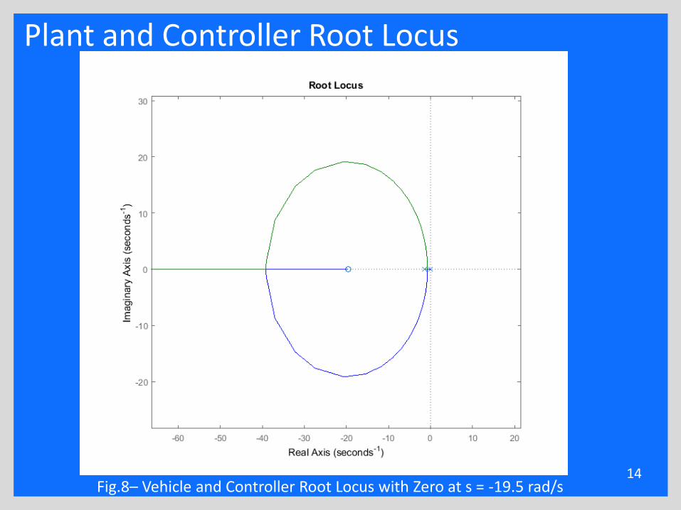
Plant and Controller Root Locus
14Fig.8– Vehicle and Controller Root Locus with Zero at s = -19.5 rad/s
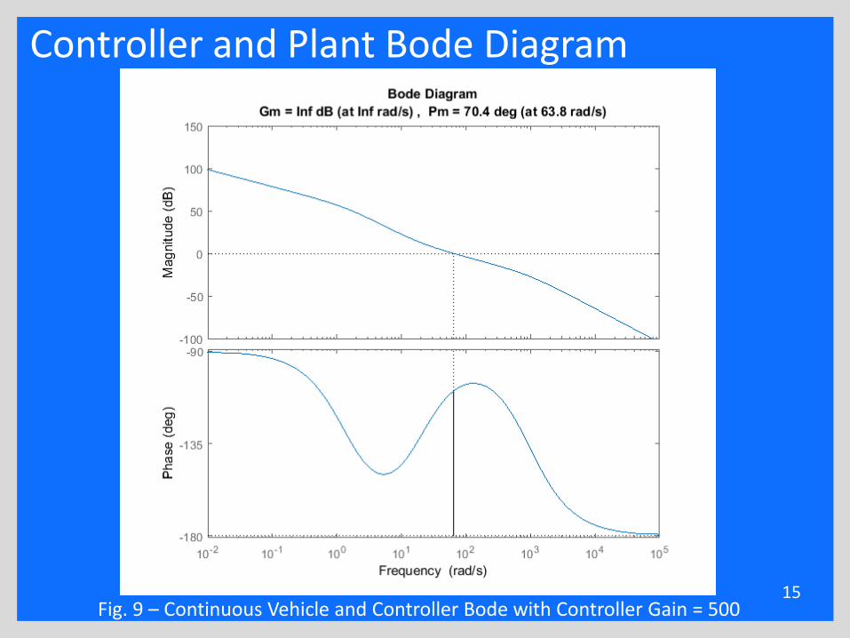
Controller and Plant Bode Diagram
15Fig. 9 – Continuous Vehicle and Controller Bode with Controller Gain = 500
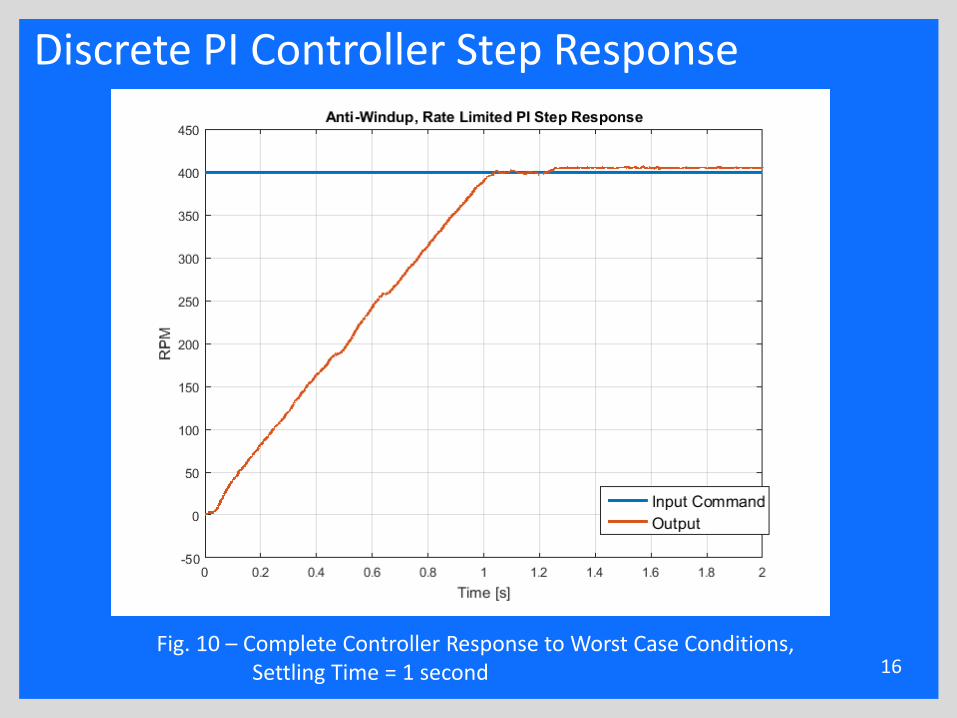
Discrete PI Controller Step Response
16Fig. 10 – Complete Controller Response to Worst Case Conditions,
Settling Time = 1 second
Presentation Outline
•Background•Benjamin Roos
•Controller Development – PI Feedback Controller•Controller Specification Verification•Current Source and Dynamic Model Matching
•Timothy De Pasion•Alexander Schmidt•Kevin Block•Conclusion
17
Disturbance Rejection Specification
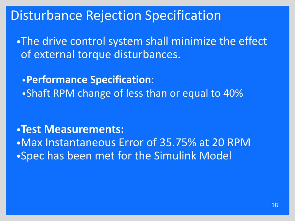
•The drive control system shall minimize the effect of external torque disturbances.
•Performance Specification:•Shaft RPM change of less than or equal to 40%
•Test Measurements:•Max Instantaneous Error of 35.75% at 20 RPM•Spec has been met for the Simulink Model
18
Disturbance Rejection Specification
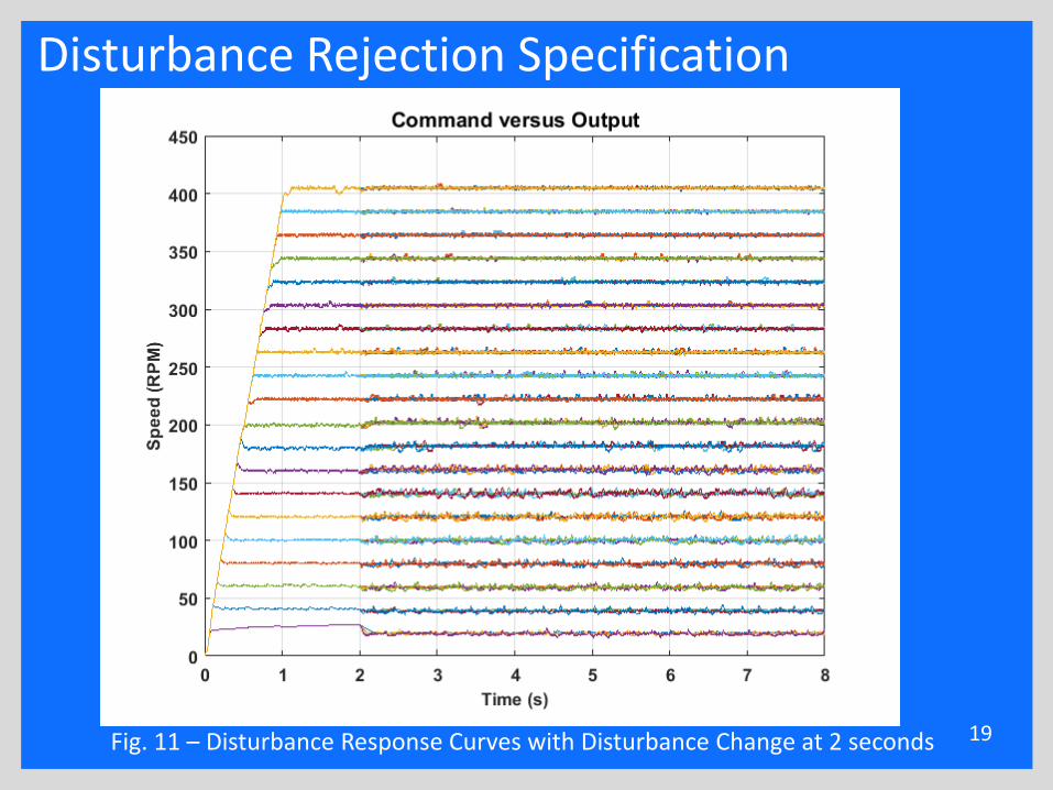
19Fig. 11 – Disturbance Response Curves with Disturbance Change at 2 seconds
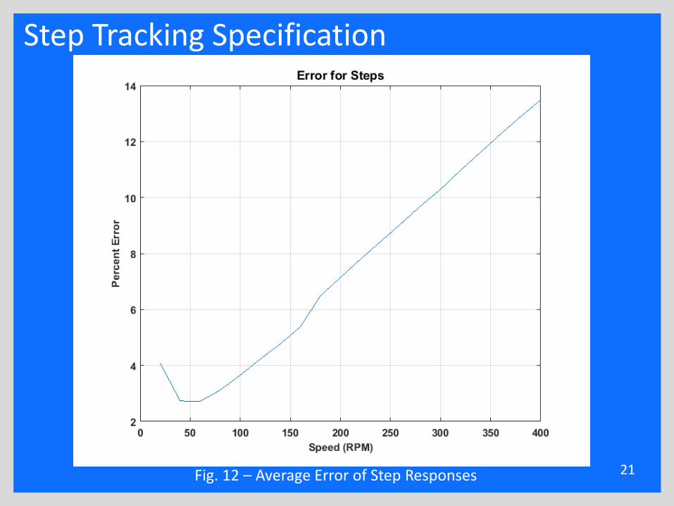
Step Tracking Specification
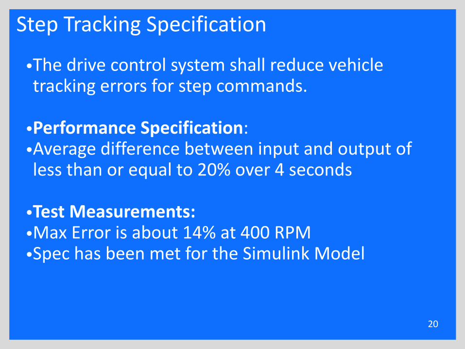
•The drive control system shall reduce vehicle tracking errors for step commands.
•Performance Specification: •Average difference between input and output of less than or equal to 20% over 4 seconds
•Test Measurements:•Max Error is about 14% at 400 RPM•Spec has been met for the Simulink Model
20
Step Tracking Specification
21Fig. 12 – Average Error of Step Responses
Ramp Tracking Specification
•The drive control system shall reduce vehicle tracking errors for ramp commands.
•Performance Specification: Average difference between input and output of less than or equal to 20% over 4 seconds
•Test Measurements:•Max Error is about 35% at 400 RPM/s
22
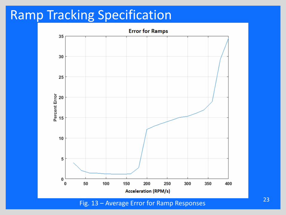
Ramp Tracking Specification
23Fig. 13 – Average Error for Ramp Responses
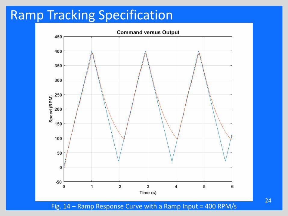
Ramp Tracking Specification
24Fig. 14 – Ramp Response Curve with a Ramp Input = 400 RPM/s
Parabolic Tracking Specification
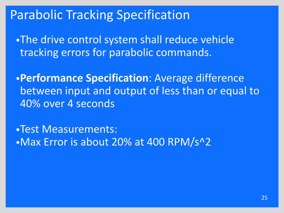
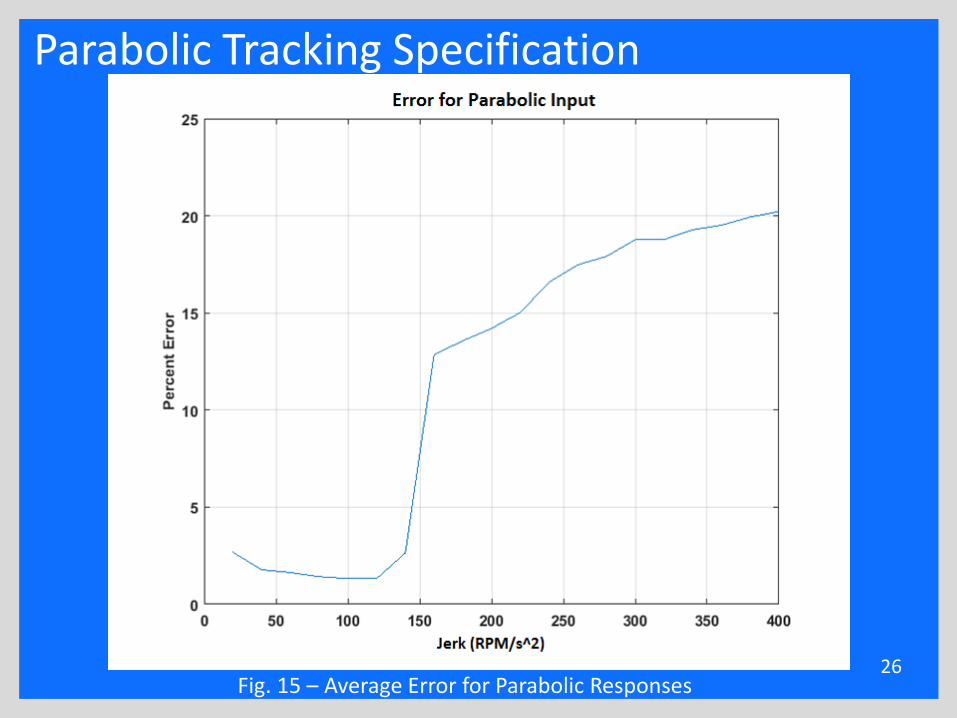
•The drive control system shall reduce vehicle tracking errors for parabolic commands.
•Performance Specification: Average difference between input and output of less than or equal to 40% over 4 seconds
•Test Measurements:•Max Error is about 20% at 400 RPM/s^2
25
Parabolic Tracking Specification
26Fig. 15 – Average Error for Parabolic Responses
Presentation Outline
•Background•Benjamin Roos
•Controller Development – PI Feedback Controller•Controller Specification Verification•Current Source and Dynamic Model Matching
•Timothy De Pasion•Alexander Schmidt•Kevin Block•Conclusion
27
Current Source Torque Disturbance Matching
28
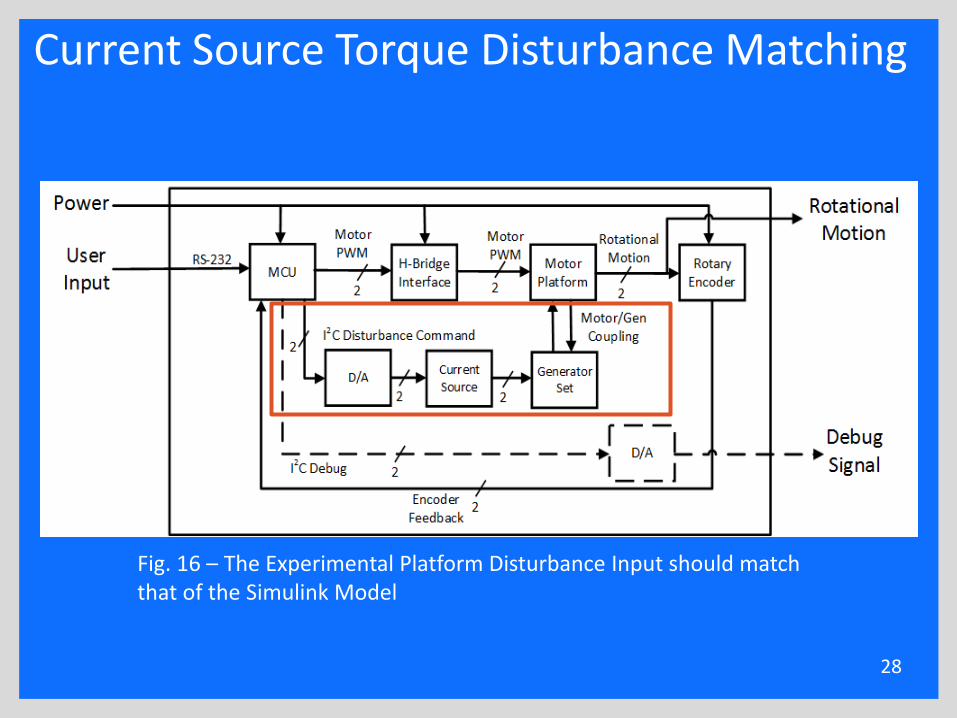
Fig. 16 – The Experimental Platform Disturbance Input should match that of the Simulink Model
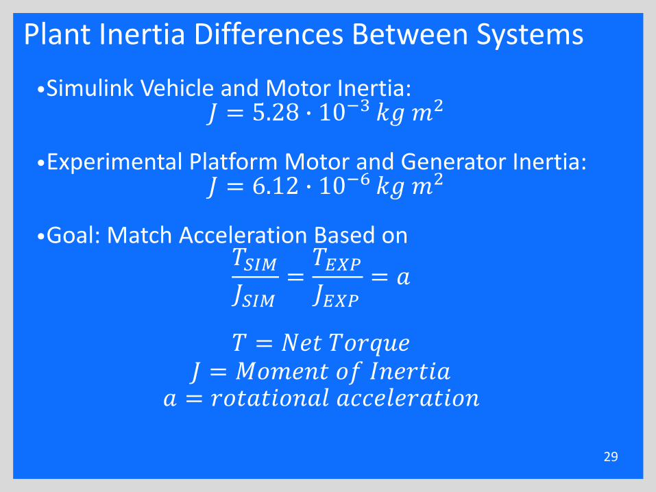
Plant Inertia Differences Between Systems
•Simulink Vehicle and Motor Inertia:𝐽 = 5.28 ∙ 10−3 𝑘𝑔 𝑚2
•Experimental Platform Motor and Generator Inertia:𝐽 = 6.12 ∙ 10−6 𝑘𝑔 𝑚2
•Goal: Match Acceleration Based on𝑇𝑆𝐼𝑀𝐽𝑆𝐼𝑀
=𝑇𝐸𝑋𝑃𝐽𝐸𝑋𝑃
= 𝑎
𝑇 = 𝑁𝑒𝑡 𝑇𝑜𝑟𝑞𝑢𝑒𝐽 = 𝑀𝑜𝑚𝑒𝑛𝑡 𝑜𝑓 𝐼𝑛𝑒𝑟𝑡𝑖𝑎
𝑎 = 𝑟𝑜𝑡𝑎𝑡𝑖𝑜𝑛𝑎𝑙 𝑎𝑐𝑐𝑒𝑙𝑒𝑟𝑎𝑡𝑖𝑜𝑛
29
Presentation Outline
•Background•Benjamin Roos•Timothy De Pasion•Alexander Schmidt•Kevin Block•Conclusion
30

Presentation Outline
•Background•Benjamin Roos•Timothy De Pasion
•Simulink Integration•Controller Development – Feed Forward•Terrain Creation•GUI Creation
•Alexander Schmidt•Kevin Block•Conclusion
31
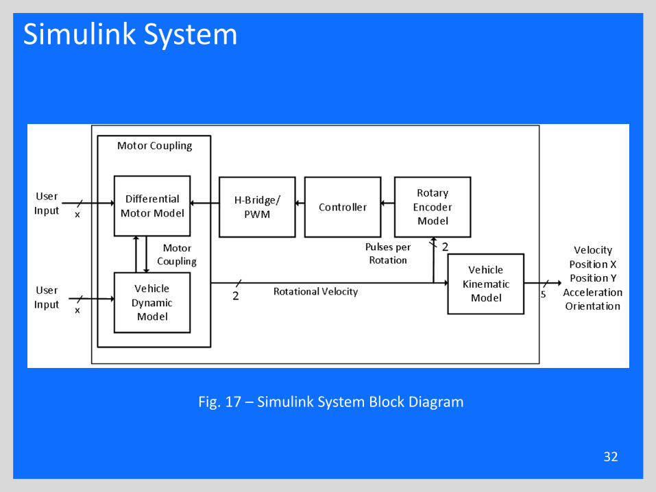
Simulink System
32
Fig. 17 – Simulink System Block Diagram
Simulink Integration
•Goal: Combine individual Simulink models into one overall model
•Problems: •Timing Problems•Model Redesign
33
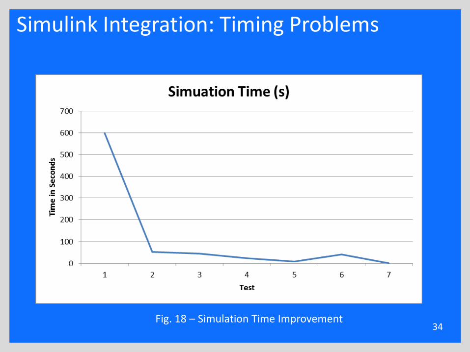
Simulink Integration: Timing Problems
34Fig. 18 – Simulation Time Improvement
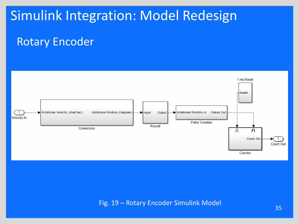
Simulink Integration: Model Redesign
Rotary Encoder
35Fig. 19 – Rotary Encoder Simulink Model
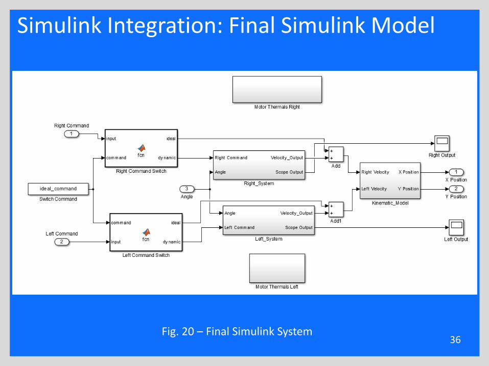
Simulink Integration: Final Simulink Model
36Fig. 20 – Final Simulink System
Presentation Outline
•Background•Benjamin Roos•Timothy De Pasion
•Simulink Integration•Controller Development – Feed Forward•Terrain Creation•GUI Creation
•Alexander Schmidt•Kevin Block•Conclusion
37
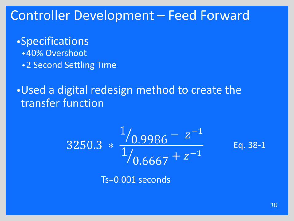
Controller Development – Feed Forward
•Specifications•40% Overshoot•2 Second Settling Time
•Used a digital redesign method to create the transfer function
38
3250.3 ∗ 1 0.9986 − 𝑧−1
1 0.6667 + 𝑧−1
Ts=0.001 seconds
Eq. 38-1
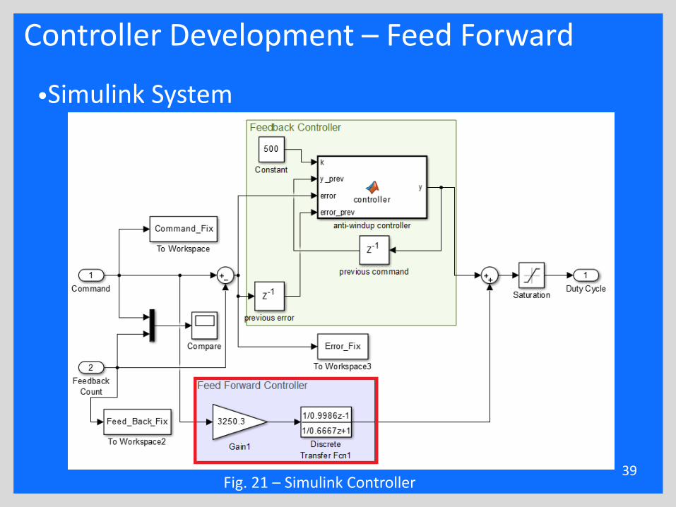
Controller Development – Feed Forward
•Simulink System
39Fig. 21 – Simulink Controller
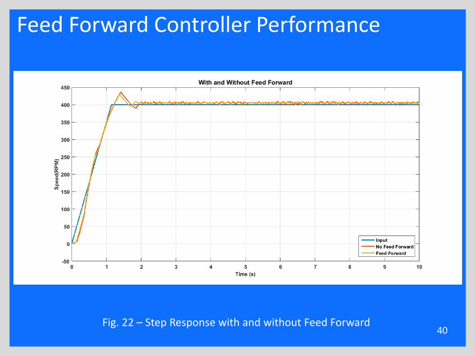
Feed Forward Controller Performance
40Fig. 22 – Step Response with and without Feed Forward
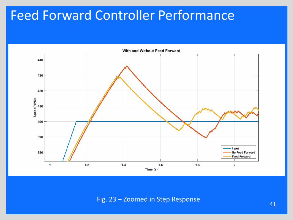
Feed Forward Controller Performance
41Fig. 23 – Zoomed in Step Response
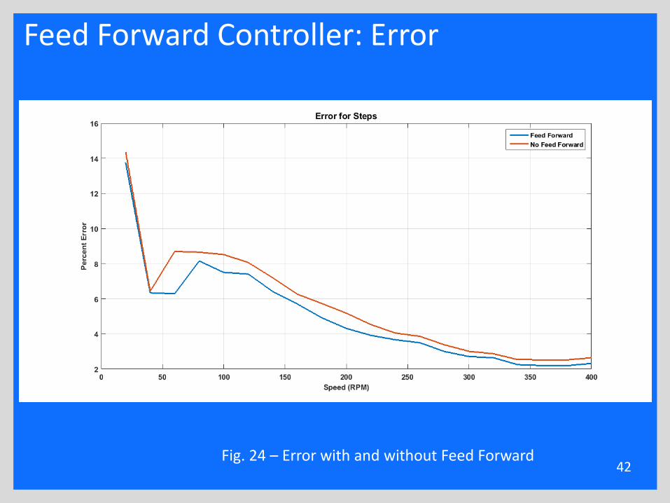
Feed Forward Controller: Error
42Fig. 24 – Error with and without Feed Forward
Presentation Outline
•Background•Benjamin Roos•Timothy De Pasion
•Simulink Integration•Controller Development – Feed Forward•Terrain Creation•GUI Creation
•Alexander Schmidt•Kevin Block•Conclusion
43
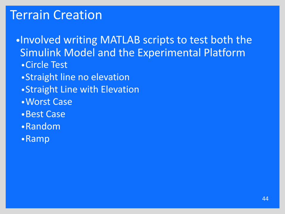
Terrain Creation
•Involved writing MATLAB scripts to test both the Simulink Model and the Experimental Platform•Circle Test•Straight line no elevation•Straight Line with Elevation•Worst Case•Best Case•Random•Ramp
44
Presentation Outline
•Background•Benjamin Roos•Timothy De Pasion
•Simulink Integration•Controller Development – Feed Forward•Experimental Platform Integration•Terrain Creation•GUI Creation
•Alexander Schmidt•Kevin Block•Conclusion
45
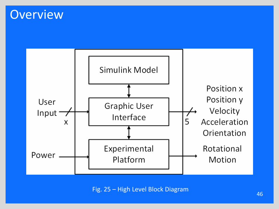
Overview
46Fig. 25 – High Level Block Diagram
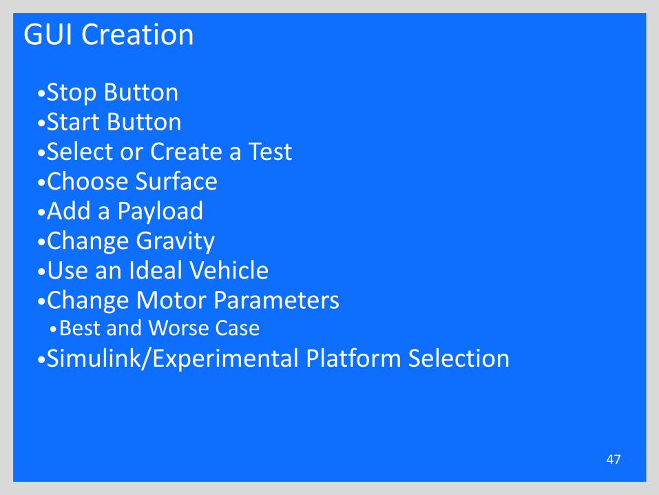
GUI Creation
•Stop Button•Start Button•Select or Create a Test•Choose Surface•Add a Payload•Change Gravity•Use an Ideal Vehicle•Change Motor Parameters
•Best and Worse Case
•Simulink/Experimental Platform Selection
47
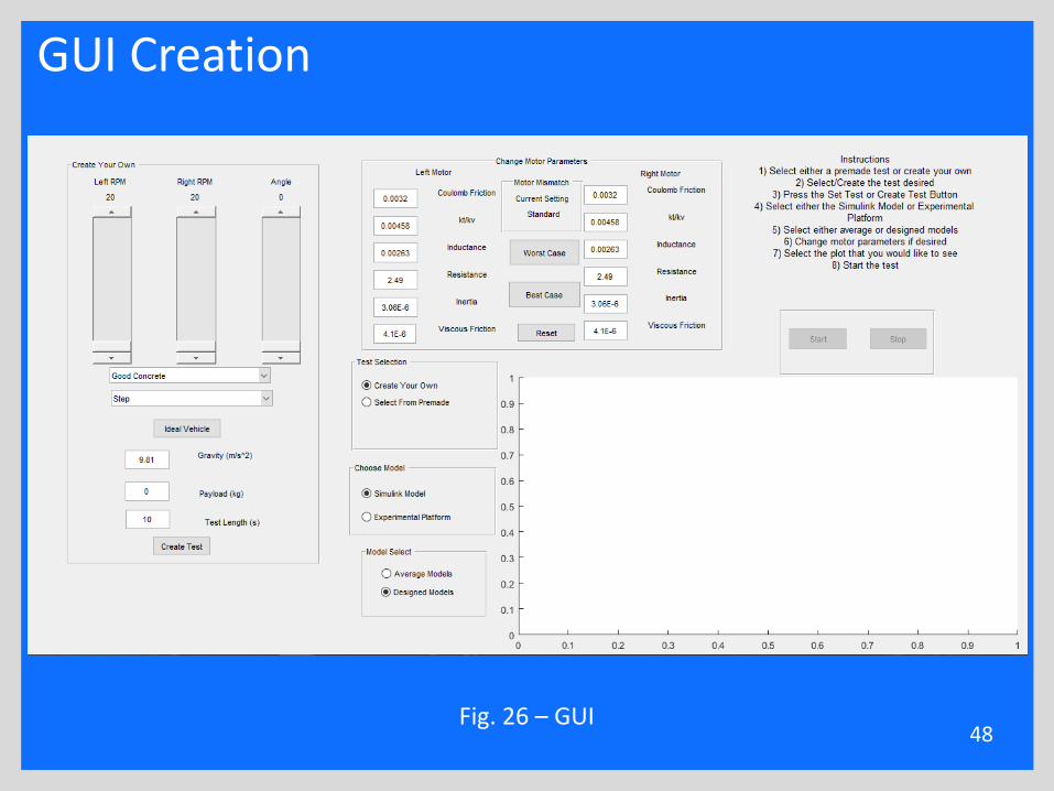
GUI Creation
48Fig. 26 – GUI
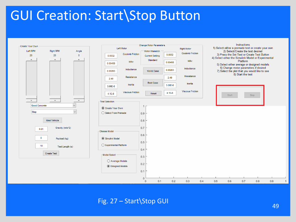
GUI Creation: Start\Stop Button
49Fig. 27 – Start\Stop GUI
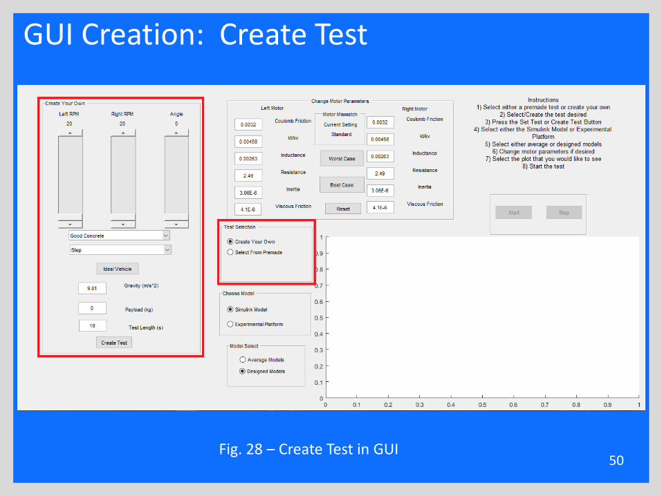
GUI Creation: Create Test
50Fig. 28 – Create Test in GUI
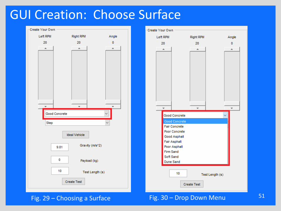
GUI Creation: Choose Surface
51Fig. 29 – Choosing a Surface Fig. 30 – Drop Down Menu
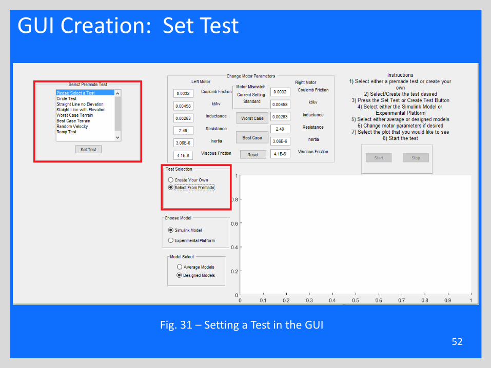
GUI Creation: Set Test
52
Fig. 31 – Setting a Test in the GUI
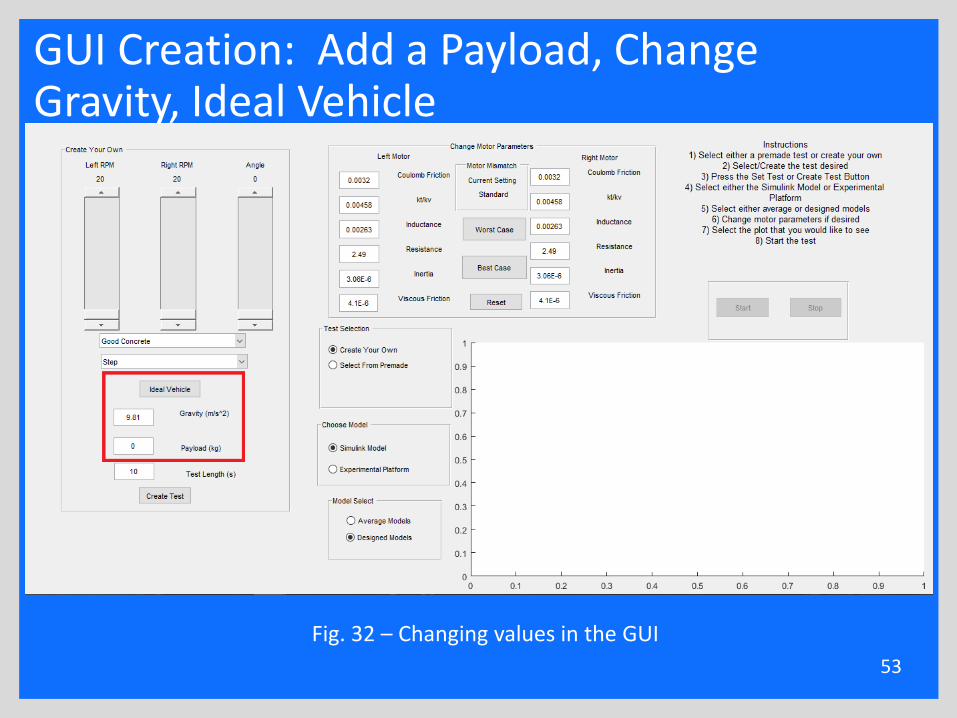
GUI Creation: Add a Payload, Change Gravity, Ideal Vehicle
53
Fig. 32 – Changing values in the GUI
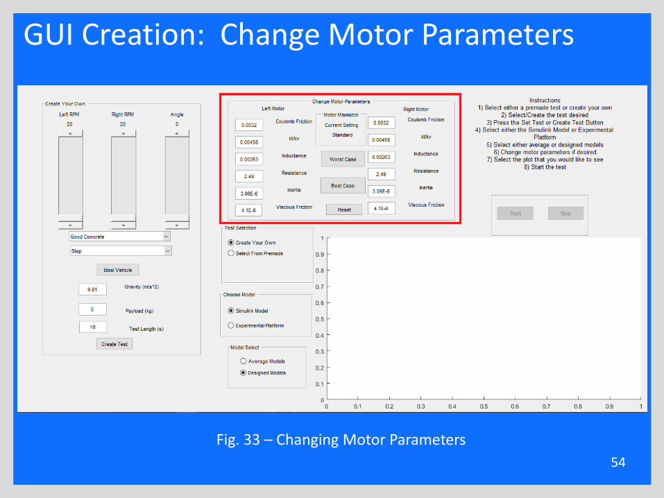
GUI Creation: Change Motor Parameters
54
Fig. 33 – Changing Motor Parameters
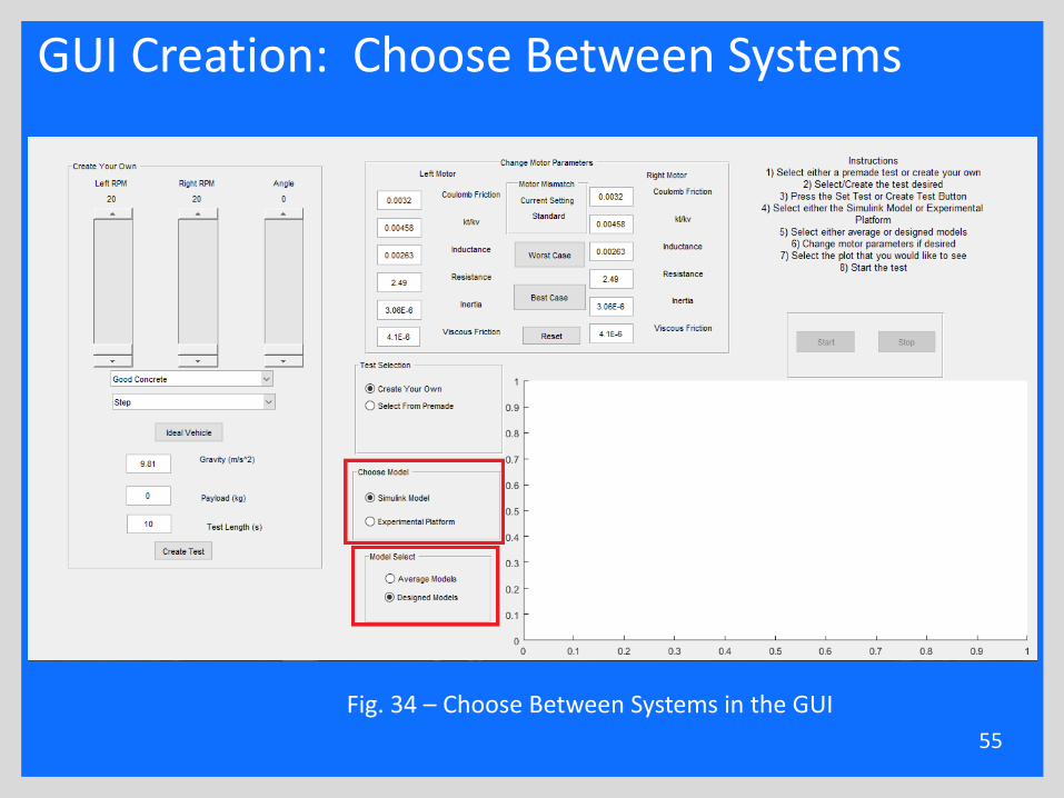
GUI Creation: Choose Between Systems
55
Fig. 34 – Choose Between Systems in the GUI
Presentation Outline
•Background•Benjamin Roos•Timothy De Pasion•Alexander Schmidt•Kevin Block•Conclusion
56
Presentation Outline
•Background•Benjamin Roos•Timothy De Pasion•Alexander Schmidt
• Motor Thermals• H-Bridge• GUI Design
•Kevin Block•Conclusion
57
Motor Thermals: 4 Sources of Heat
•Resistance in the windings
•Coulomb Friction
•Viscous Friction
•Dynamic Loads
58
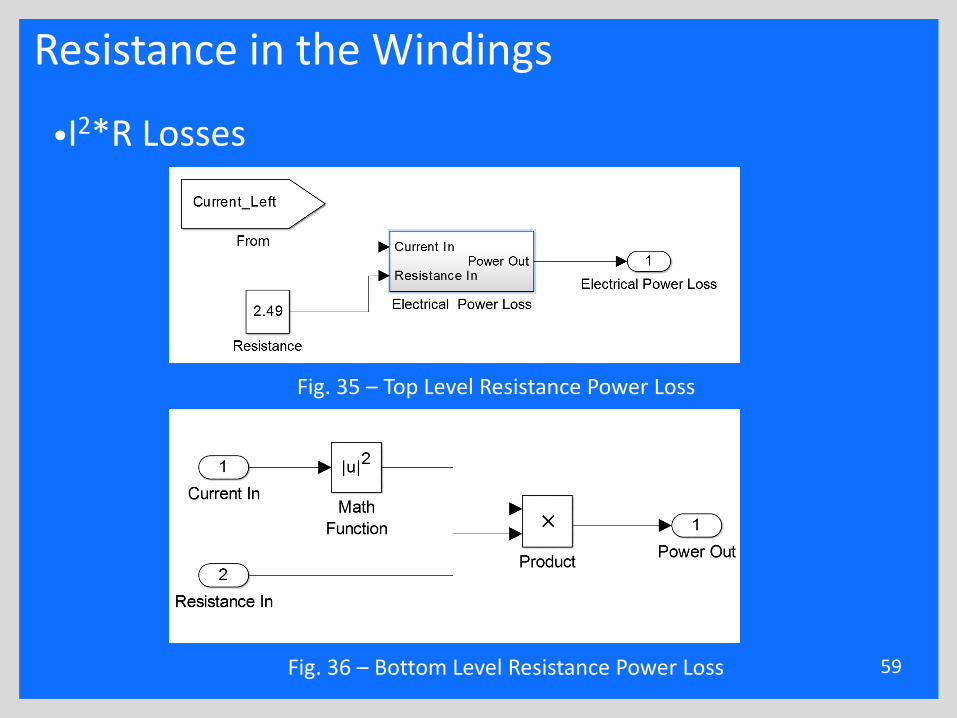
Resistance in the Windings
•I2*R Losses
59
Fig. 35 – Top Level Resistance Power Loss
Fig. 36 – Bottom Level Resistance Power Loss
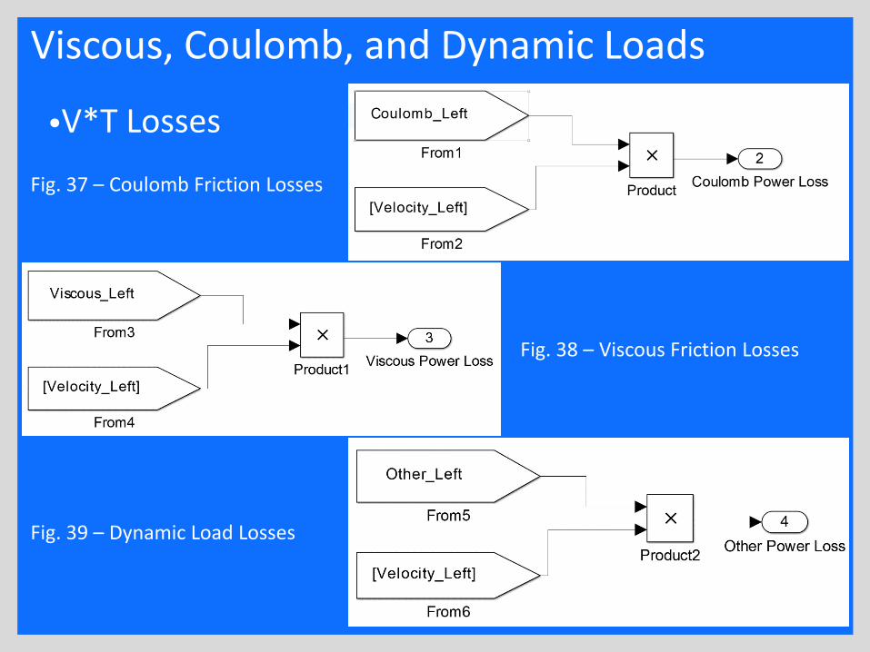
Viscous, Coulomb, and Dynamic Loads
•V*T Losses
60
Fig. 37 – Coulomb Friction Losses
Fig. 39 – Dynamic Load Losses
Fig. 38 – Viscous Friction Losses
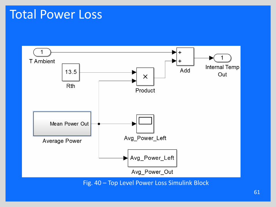
Total Power Loss
61
Fig. 40 – Top Level Power Loss Simulink Block
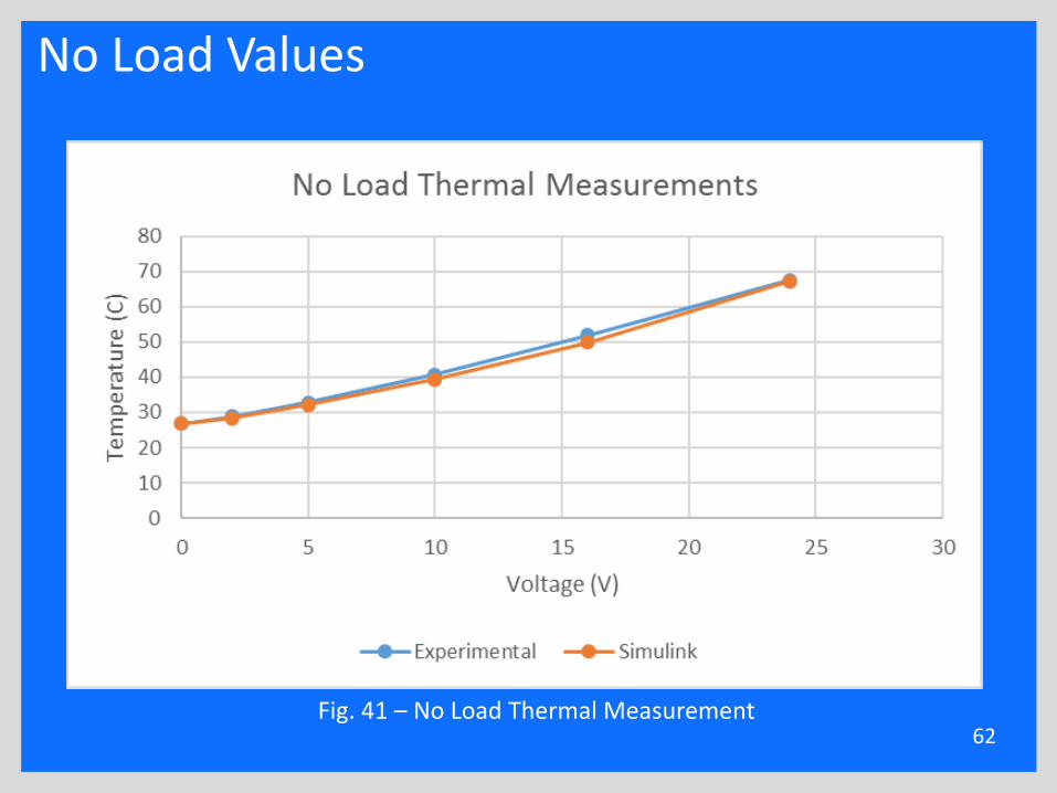
No Load Values
62Fig. 41 – No Load Thermal Measurement
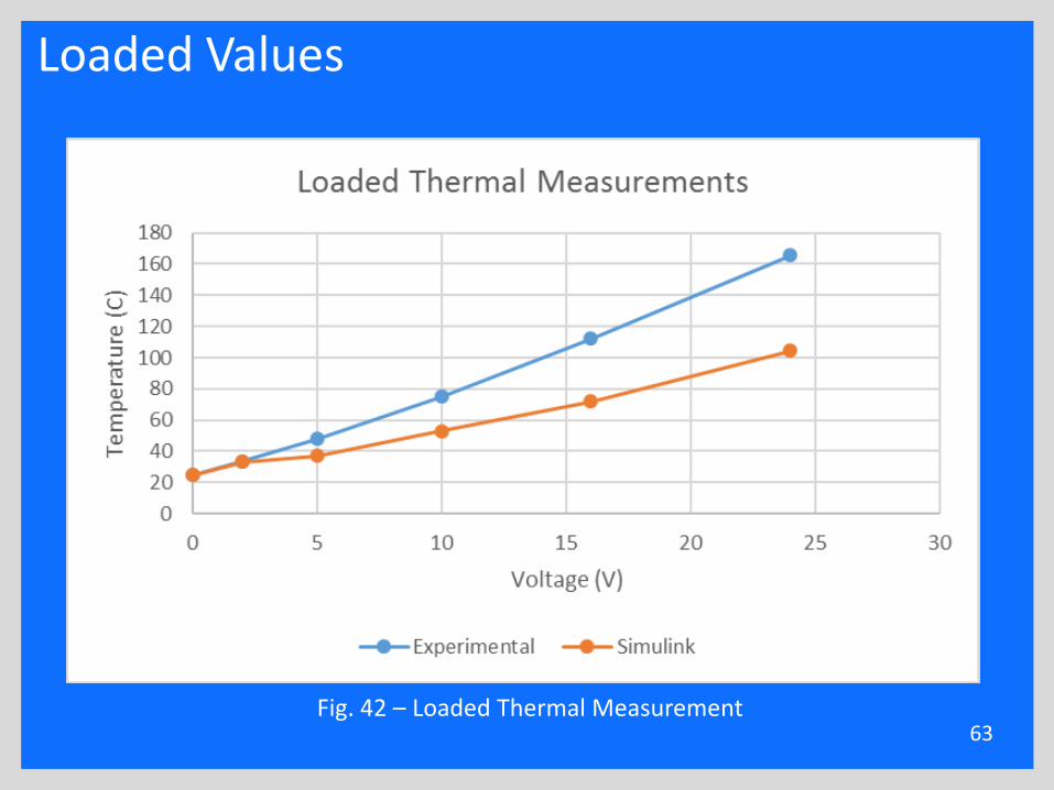
Loaded Values
63Fig. 42 – Loaded Thermal Measurement

Presentation Outline
•Background•Benjamin Roos•Timothy De Pasion•Alexander Schmidt
• Motor Thermals• H-Bridge• GUI Design
•Kevin Block•Conclusion
64
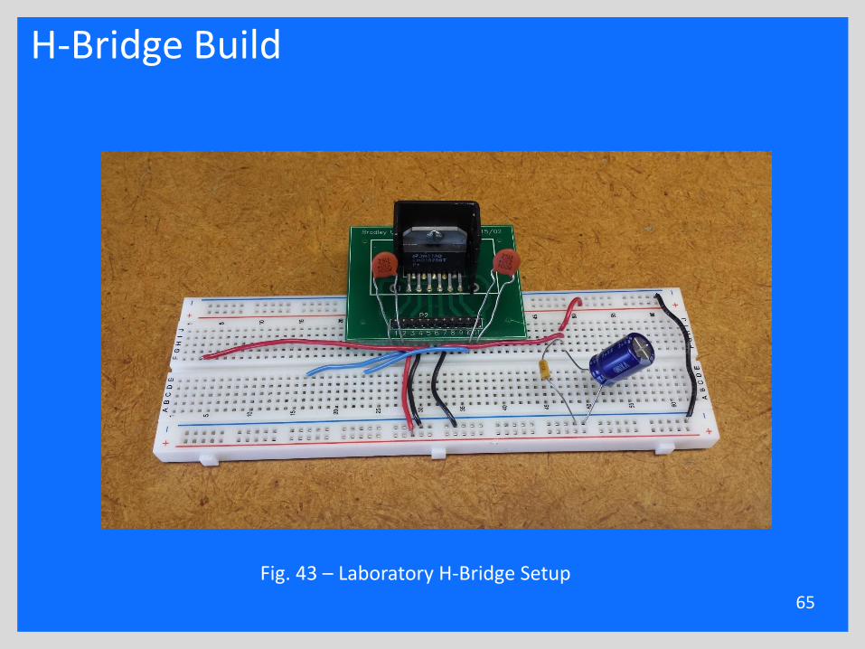
H-Bridge Build
65
Fig. 43 – Laboratory H-Bridge Setup
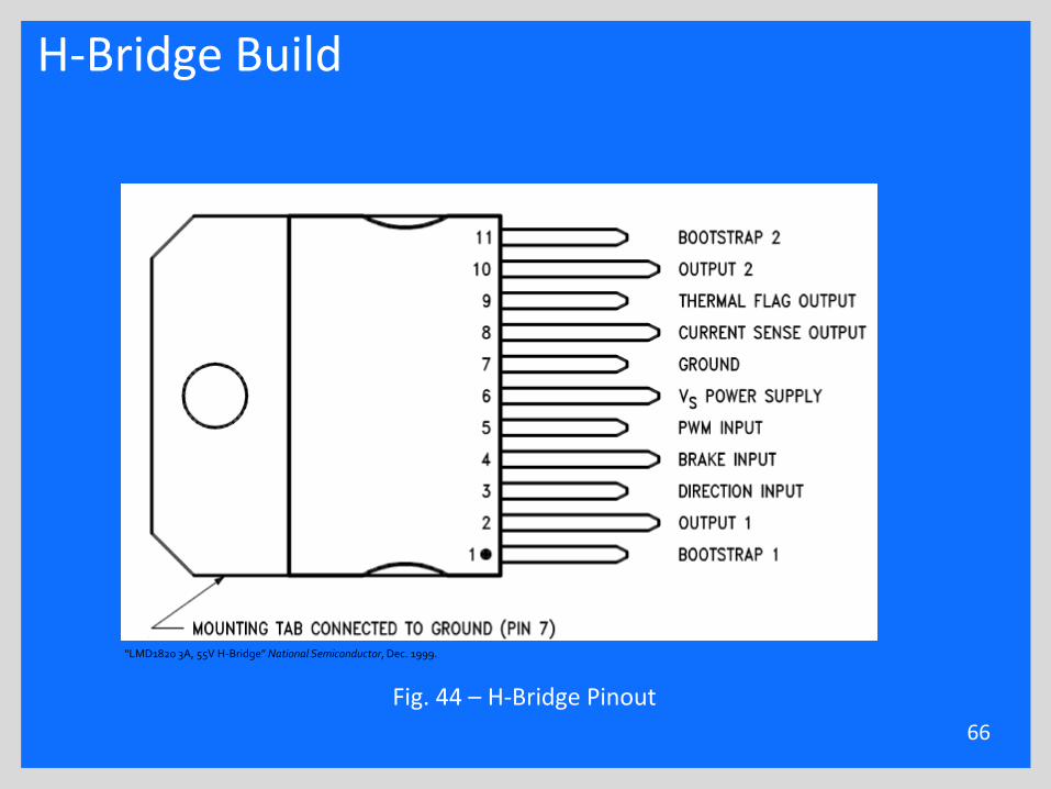
H-Bridge Build
66
Fig. 44 – H-Bridge Pinout
“LMD1820 3A, 55V H-Bridge” National Semiconductor, Dec. 1999.
H-Bridge Thermals
•Total Power of H-BridgePTotal = PQ + PCOND + PSW [EQ – 67.1]
PQ = Quiescent Power Dissipation
PCOND = Conductive Power Dissipation
PSW = Switching Power Dissipation
67
Quiescent Power Dissipation
PQ = IS * VCC [EQ – 68.1]
IS = Quiescent Current
VCC = Supply Voltage
68
Conductive Power Dissipation
PCOND = 2 * I2RMS * RDS (ON) [EQ – 69.1]
IRMS = RMS Current
RDS (ON) = On Resistance of the Power Switch
69
Switching Power Dissipation
PSW = (EON + EOFF) * F [EQ – 70.1]
EON = Turn On Energy
EOFF = Turn Off Energy
F = Switching Frequency
70
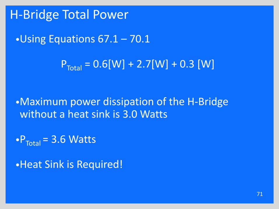
H-Bridge Total Power
•Using Equations 67.1 – 70.1
PTotal = 0.6[W] + 2.7[W] + 0.3 [W]
•Maximum power dissipation of the H-Bridge without a heat sink is 3.0 Watts
•PTotal = 3.6 Watts
•Heat Sink is Required!
71
Presentation Outline
•Background•Benjamin Roos•Timothy De Pasion•Alexander Schmidt
• Motor Thermals• H-Bridge• GUI Design
•Kevin Block•Conclusion
72
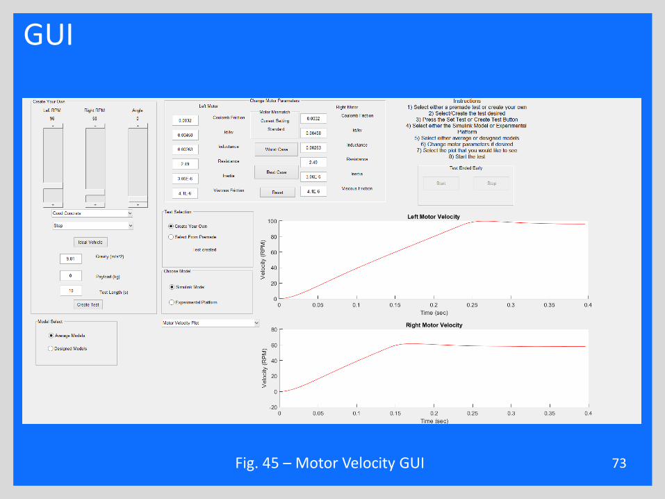
GUI
73Fig. 45 – Motor Velocity GUI
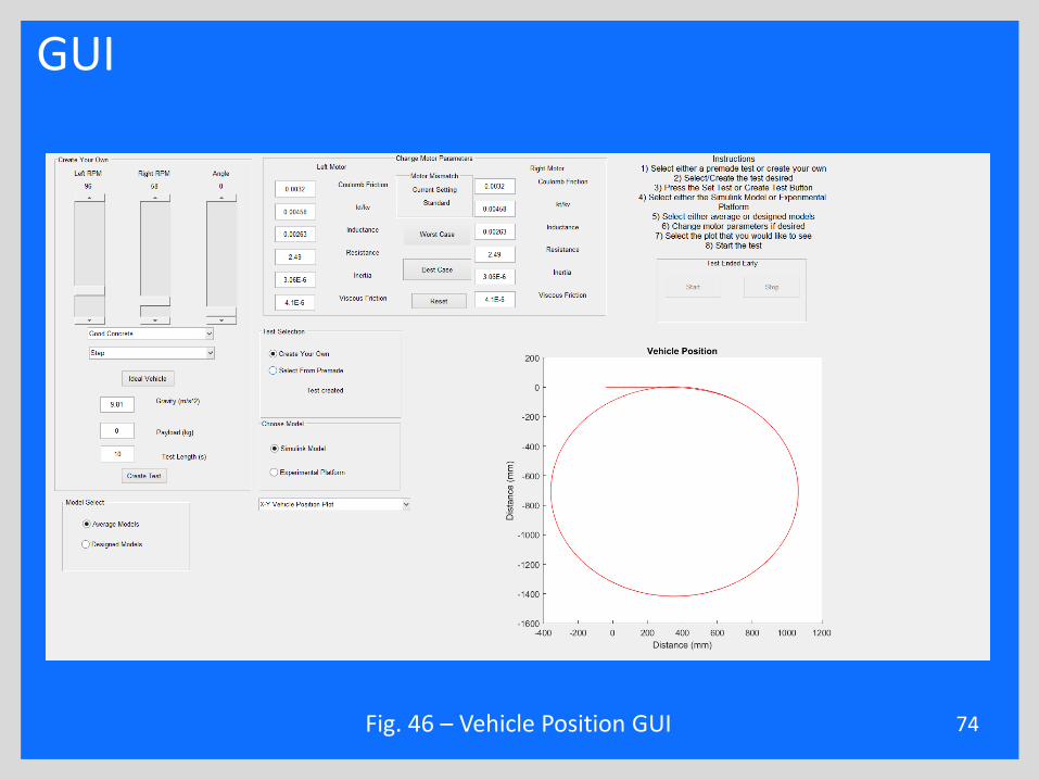
GUI
74Fig. 46 – Vehicle Position GUI
Presentation Outline
•Background•Benjamin Roos•Timothy De Pasion•Alexander Schmidt•Kevin Block•Conclusion
75
Presentation Outline
•Background•Benjamin Roos•Timothy De Pasion•Alexander Schmidt•Kevin Block
•Rotary Encoder Resolution•Controller Software•Interrupt Timing
•Conclusion
76
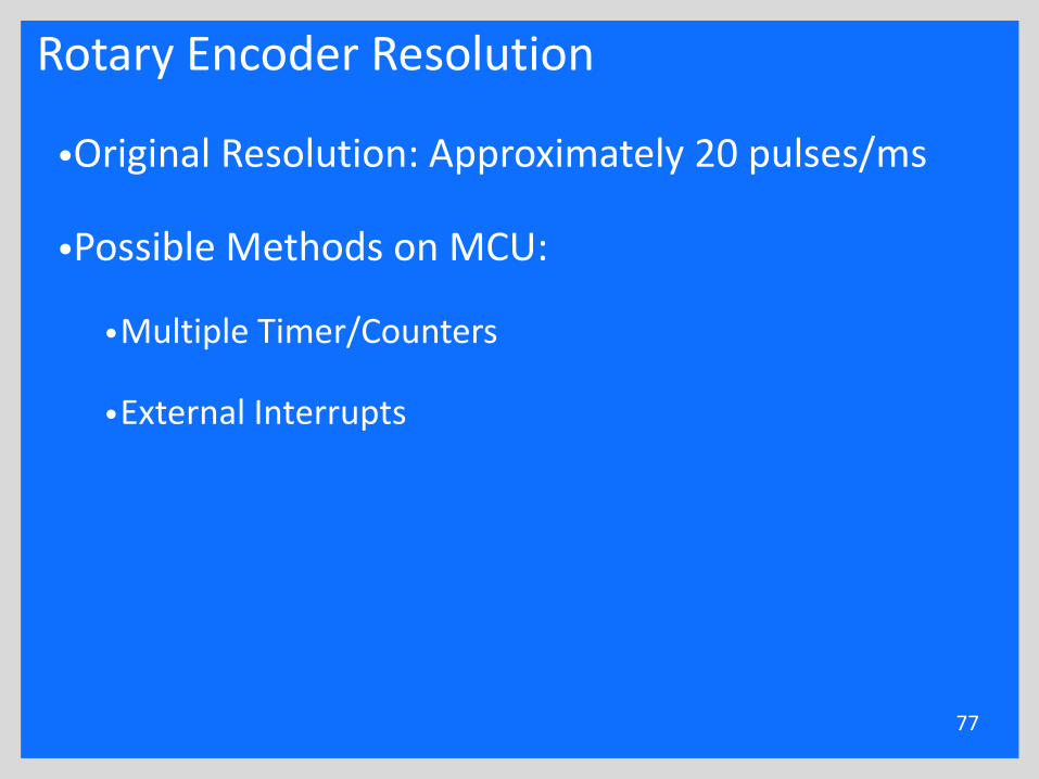
Rotary Encoder Resolution
77
•Original Resolution: Approximately 20 pulses/ms
•Possible Methods on MCU:
•Multiple Timer/Counters
•External Interrupts
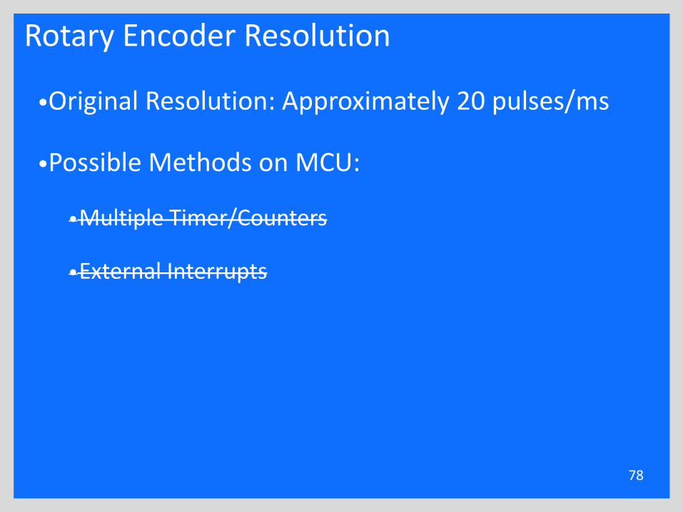
Rotary Encoder Resolution
78
•Original Resolution: Approximately 20 pulses/ms
•Possible Methods on MCU:
•Multiple Timer/Counters
•External Interrupts
Rotary Encoder Resolution
79
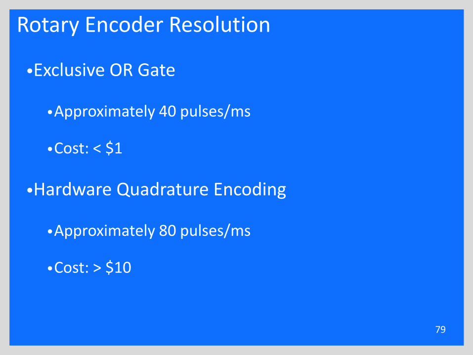
•Exclusive OR Gate
•Approximately 40 pulses/ms
•Cost: < $1
•Hardware Quadrature Encoding
•Approximately 80 pulses/ms
•Cost: > $10
Presentation Outline
•Background•Benjamin Roos•Timothy De Pasion•Alexander Schmidt•Kevin Block
•Rotary Encoder Resolution•Controller Software•Interrupt Timing
•Conclusion
80
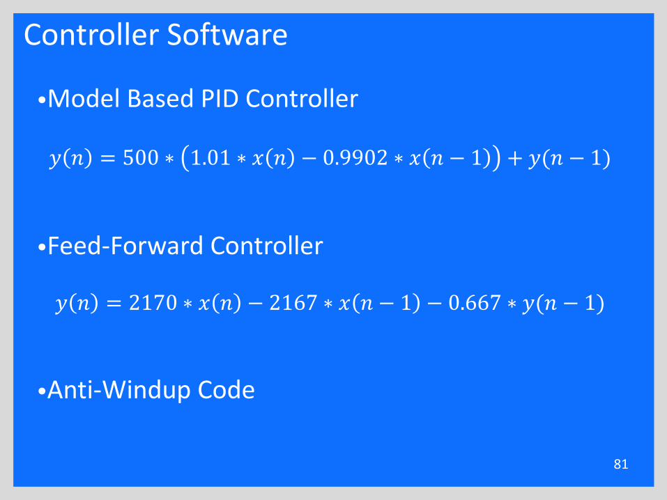
Controller Software
81
•Model Based PID Controller
𝑦 𝑛 = 500 ∗ 1.01 ∗ 𝑥 𝑛 − 0.9902 ∗ 𝑥 𝑛 − 1 + 𝑦(𝑛 − 1)
•Feed-Forward Controller
𝑦 𝑛 = 2170 ∗ 𝑥 𝑛 − 2167 ∗ 𝑥 𝑛 − 1 − 0.667 ∗ 𝑦(𝑛 − 1)
•Anti-Windup Code
Controller Software
82
0 2 4 6 8 10 12 14 16 18 200
2
4
6
8
10
12
14
16
Time [s]
Inp
ut
(Red
) an
d O
utp
ut
(Gre
en
) [P
uls
es/m
s]
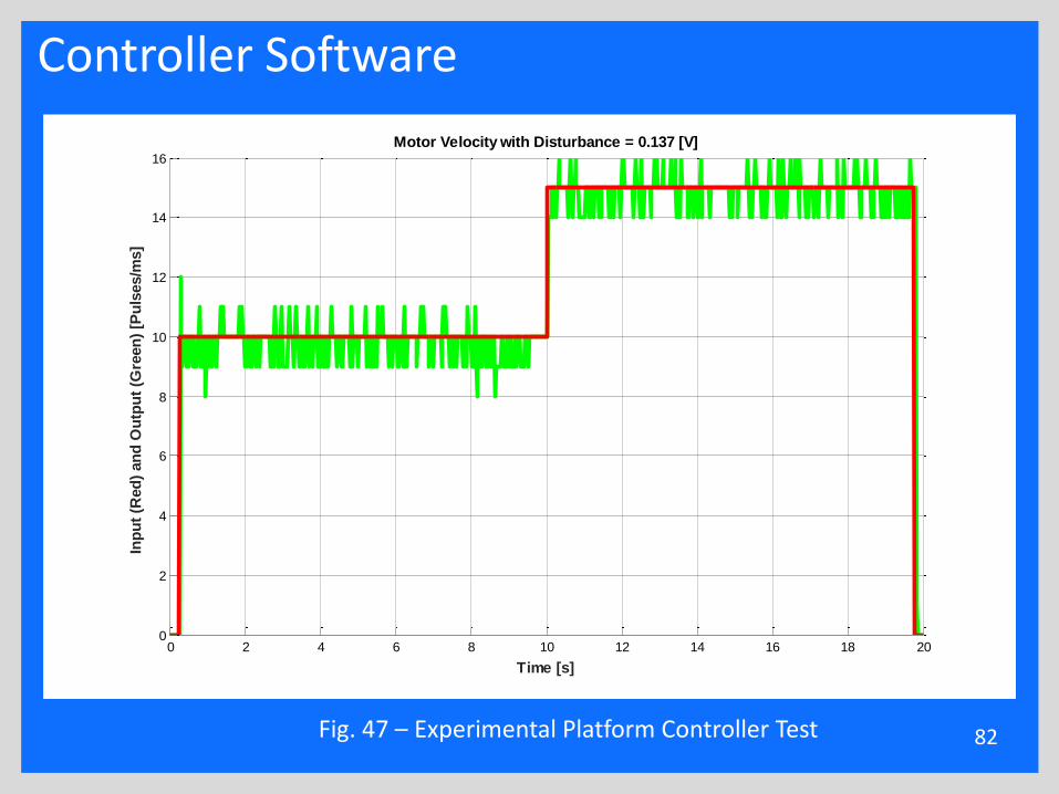
Motor Velocity with Disturbance = 0.137 [V]
Fig. 47 – Experimental Platform Controller Test
Presentation Outline
•Background•Benjamin Roos•Timothy De Pasion•Alexander Schmidt•Kevin Block
•Rotary Encoder Resolution•Controller Software•Interrupt Timing
•Conclusion
83
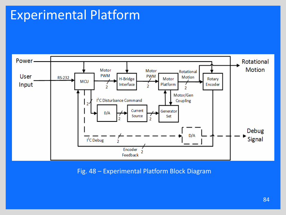
Experimental Platform
84
Fig. 48 – Experimental Platform Block Diagram
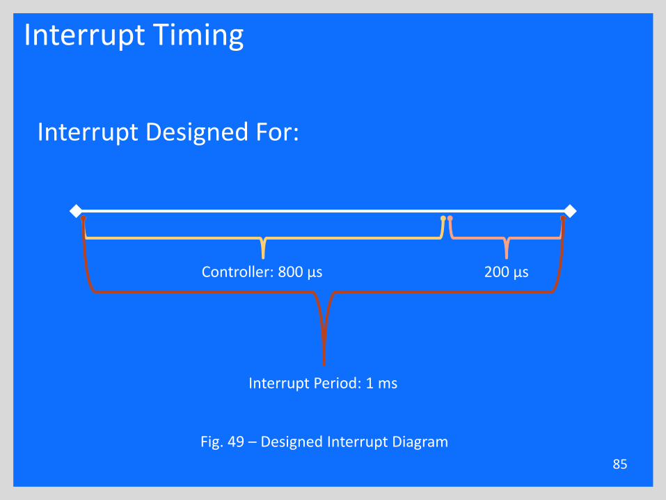
Interrupt Timing
85
Interrupt Designed For:
Controller: 800 μs 200 μs
Interrupt Period: 1 ms
Fig. 49 – Designed Interrupt Diagram
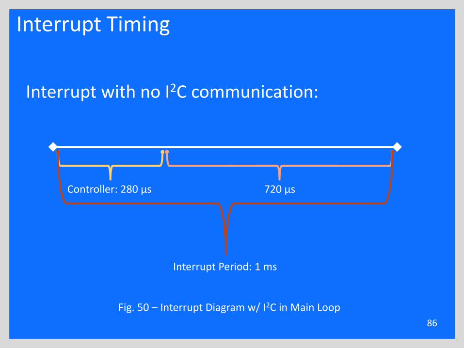
Interrupt Timing
86
Interrupt with no I2C communication:
Controller: 280 μs 720 μs
Interrupt Period: 1 ms
Fig. 50 – Interrupt Diagram w/ I2C in Main Loop
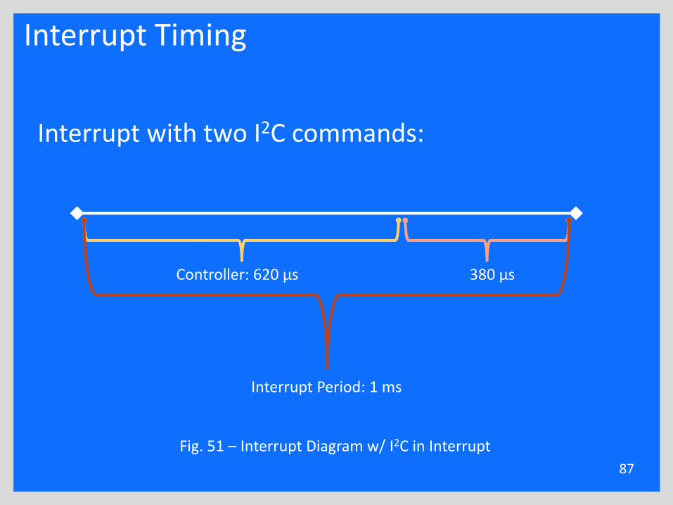
Interrupt Timing
87
Interrupt with two I2C commands:
Controller: 620 μs 380 μs
Interrupt Period: 1 ms
Fig. 51 – Interrupt Diagram w/ I2C in Interrupt
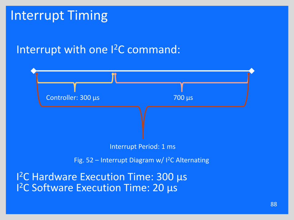
Interrupt Timing
88
Interrupt with one I2C command:
I2C Hardware Execution Time: 300 μsI2C Software Execution Time: 20 μs
Controller: 300 μs 700 μs
Interrupt Period: 1 ms
Fig. 52 – Interrupt Diagram w/ I2C Alternating
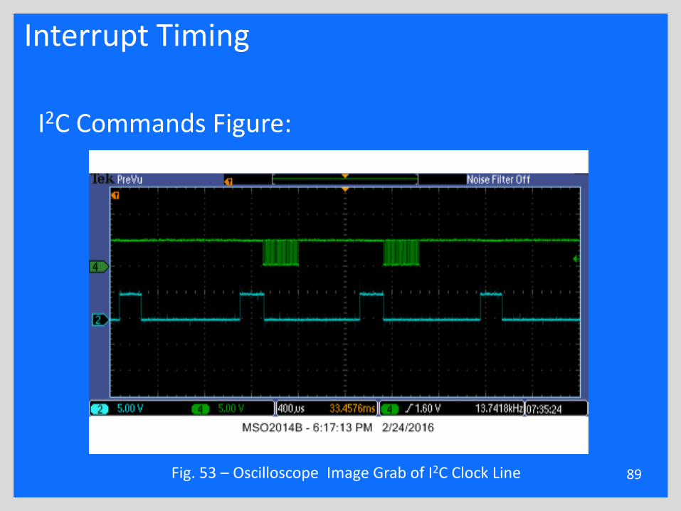
Interrupt Timing
89
I2C Commands Figure:
Fig. 53 – Oscilloscope Image Grab of I2C Clock Line
Presentation Outline
•Background•Benjamin Roos•Timothy De Pasion•Alexander Schmidt•Kevin Block•Conclusion
90
Conclusion
•Benjamin has completed:•Anti Windup Controller•Rate Limiting•Controller Development•Simulink and Experimental Platform Torque Matching in progress
91
Conclusion
•Timothy has completed:•Simulink Integration•Feed Forward Controller•Terrain Creation•GUI Creation
92
Conclusion
•Alexander has completed:•Motor Thermals•H-Bridge Heatsink•GUI Creation
93
Conclusion
•Kevin has completed:•Controller Code
•Model Based PID Controller•Feed Forward Controller•Anti Windup Code for Feedback Controller
•Doubled Resolution•Interrupt Timing
94
Objectives
•Simulink System Integration Complete ✓
•Controller Development Complete ✓
•Controller Code Written ✓
•Experimental Platform Integration Complete ✓
•Simulink GUI Complete ✓
•System Integration in Progress ✓
•System Testing in Progress ✓
95
Summary
•On schedule for project completion
•Final Step is Integration and Testing
96
Design of a Simulink-Based Control
Workstation for Mobile Wheeled Vehicles with
Variable-Velocity Differential Motor Drives
Kevin Block, Timothy De Pasion, Benjamin Roos, Alexander SchmidtGary Dempsey
Bradley University Electrical and Computer Engineering Department
March 1, 2016
Appendix Slides
•Benjamin Roos•Timothy De Pasion•Alex Schmidt
98
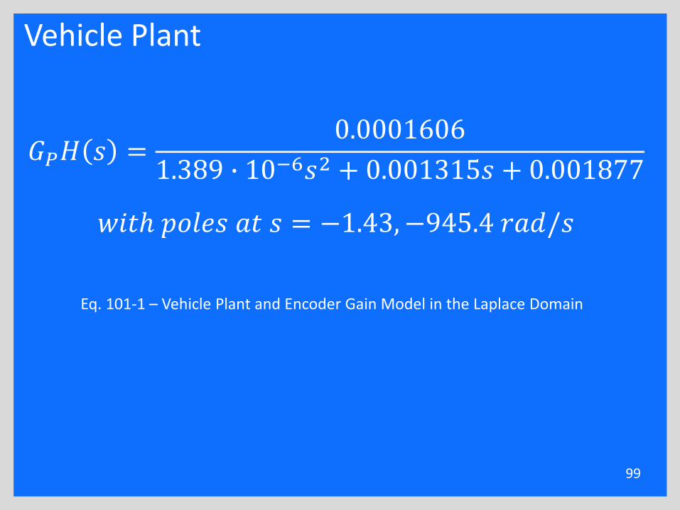
Vehicle Plant
99
𝐺𝑃𝐻 𝑠 =0.0001606
1.389 ∙ 10−6𝑠2 + 0.001315𝑠 + 0.001877
𝑤𝑖𝑡ℎ 𝑝𝑜𝑙𝑒𝑠 𝑎𝑡 𝑠 = −1.43, −945.4 𝑟𝑎𝑑/𝑠
Eq. 101-1 – Vehicle Plant and Encoder Gain Model in the Laplace Domain
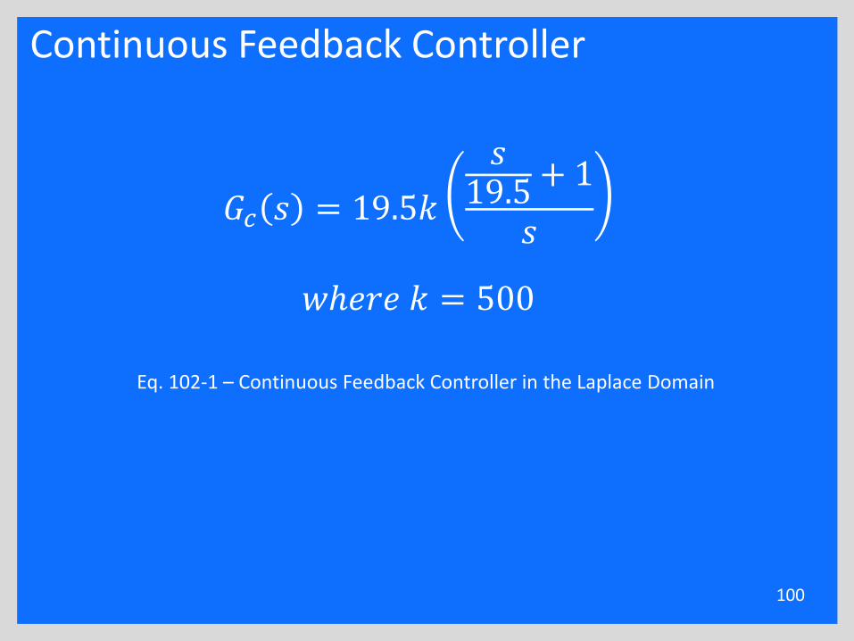
Continuous Feedback Controller
𝐺𝑐 𝑠 = 19.5𝑘
𝑠19.5
+ 1
𝑠
𝑤ℎ𝑒𝑟𝑒 𝑘 = 500
100
Eq. 102-1 – Continuous Feedback Controller in the Laplace Domain
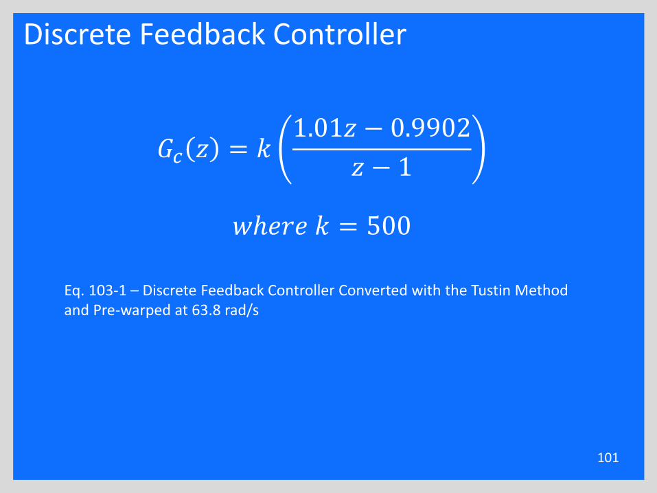
Discrete Feedback Controller
101
𝐺𝑐 𝑧 = 𝑘1.01𝑧 − 0.9902
𝑧 − 1
𝑤ℎ𝑒𝑟𝑒 𝑘 = 500
Eq. 103-1 – Discrete Feedback Controller Converted with the Tustin Method and Pre-warped at 63.8 rad/s
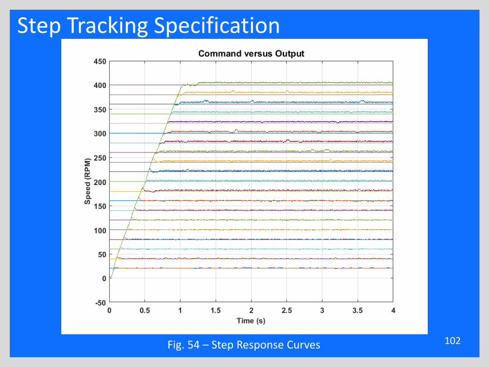
Step Tracking Specification
102Fig. 54 – Step Response Curves
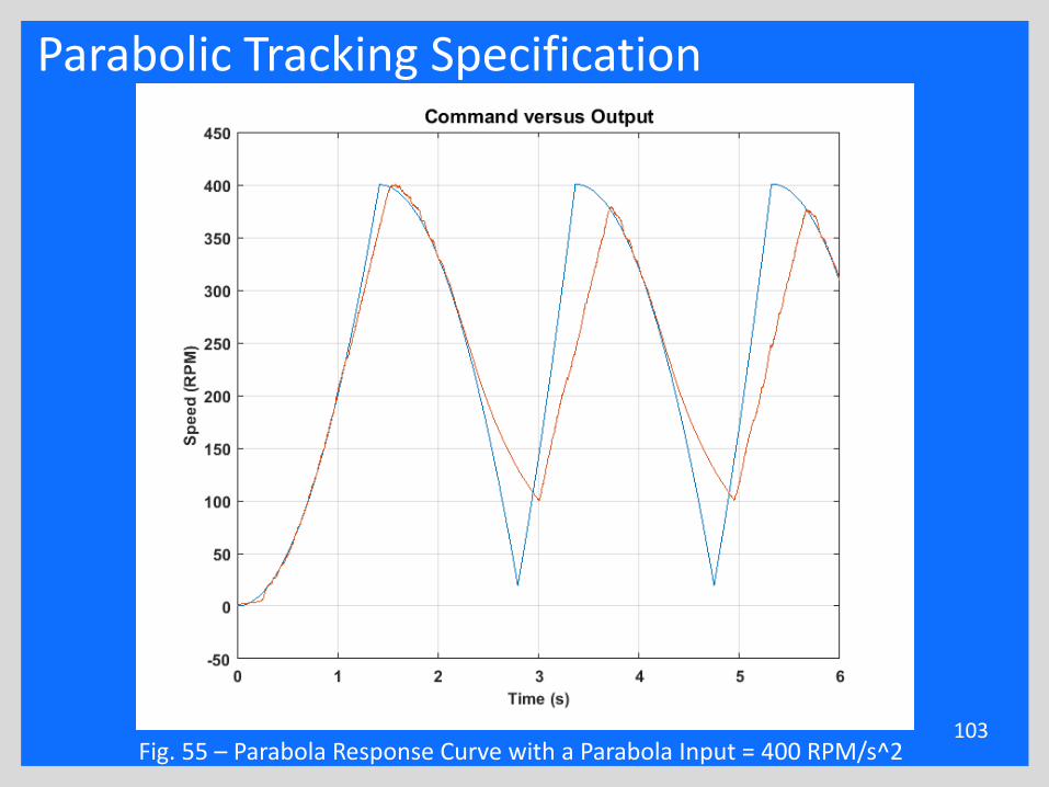
Parabolic Tracking Specification
103Fig. 55 – Parabola Response Curve with a Parabola Input = 400 RPM/s^2
Appendix Slides
•Benjamin Roos•Timothy De Pasion•Alex Schmidt
104
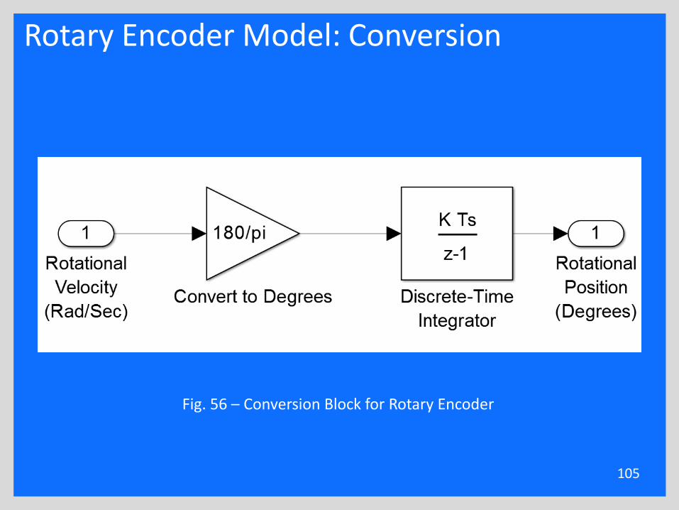
Rotary Encoder Model: Conversion
105
Fig. 56 – Conversion Block for Rotary Encoder
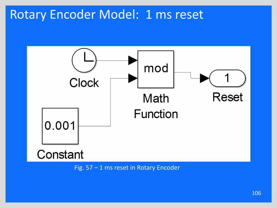
Rotary Encoder Model: 1 ms reset
106
Fig. 57 – 1 ms reset in Rotary Encoder
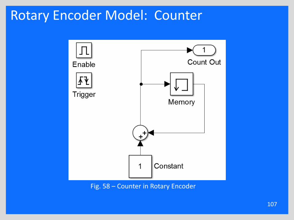
Rotary Encoder Model: Counter
107
Fig. 58 – Counter in Rotary Encoder
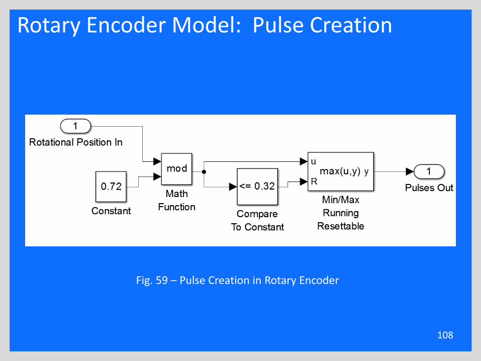
Rotary Encoder Model: Pulse Creation
108
Fig. 59 – Pulse Creation in Rotary Encoder
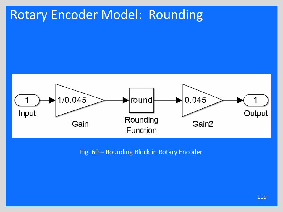
Rotary Encoder Model: Rounding
109
Fig. 60 – Rounding Block in Rotary Encoder
Appendix Slides
•Benjamin Roos•Timothy De Pasion•Alex Schmidt
110
GUI Display
•X-Y Vehicle Position Plot•Motor Velocity Plot•Current Plot•Motor Acceleration Plot•Vehicle Velocity Plot•Vehicle Acceleration Plot•Command Plot•Error Signal Plot•Feedback Signal Plot•PWM Output Plot•Feed-Forward Command Plot
111