Embed Size (px)
Citation preview
Contents
1 Introduction 1
1.1 Outline of the thesis . . . . . . . . . . . . . . . . . . . . . . . . . . . . . . . 3
1.1.1 Chapter 2: Network theory . . . . . . . . . . . . . . . . . . . . . . . 3
1.1.2 Chapter 3: WirelessHART . . . . . . . . . . . . . . . . . . . . . . . . 3
1.1.3 Chapter 4: Introduction to TrueTime . . . . . . . . . . . . . . . . . 3
1.1.4 Chapter 5: New functions in the wireless network block . . . . . . . 3
1.1.5 Chapter 6: Delay compensation . . . . . . . . . . . . . . . . . . . . . 4
1.1.6 Chapter 7: Conclusions . . . . . . . . . . . . . . . . . . . . . . . . . 4
2 Network theory 5
2.1 The Open System Interconnection model (OSI) . . . . . . . . . . . . . . . . 5
2.1.1 The OSI basic structure . . . . . . . . . . . . . . . . . . . . . . . . . 5
2.2 The Medium Access Control (MAC) protocol . . . . . . . . . . . . . . . . . 8
2.2.1 ALOHA . . . . . . . . . . . . . . . . . . . . . . . . . . . . . . . . . . 8
2.2.2 Carrier Sense Multiple Access Protocols (CSMA) . . . . . . . . . . . 9
2.2.3 Time Division Multiple Access (TDMA) . . . . . . . . . . . . . . . . 10
2.2.4 Token Bus . . . . . . . . . . . . . . . . . . . . . . . . . . . . . . . . . 10
2.2.5 Token Ring . . . . . . . . . . . . . . . . . . . . . . . . . . . . . . . . 11
2.3 The IEEE 802 standards . . . . . . . . . . . . . . . . . . . . . . . . . . . . . 12
2.3.1 Bluetooth/IEEE 802.15.1 . . . . . . . . . . . . . . . . . . . . . . . . 12
2.3.2 IEEE 802.11 . . . . . . . . . . . . . . . . . . . . . . . . . . . . . . . 13
2.3.3 IEEE 802.15.4 . . . . . . . . . . . . . . . . . . . . . . . . . . . . . . 14
2.3.4 ZigBee . . . . . . . . . . . . . . . . . . . . . . . . . . . . . . . . . . . 16
2.3.5 WirelessHART . . . . . . . . . . . . . . . . . . . . . . . . . . . . . . 16
i
CONTENTS
3 WirelessHART 19
3.1 Introduction . . . . . . . . . . . . . . . . . . . . . . . . . . . . . . . . . . . . 19
3.2 A brief view of WirelessHART . . . . . . . . . . . . . . . . . . . . . . . . . 19
3.3 MAC Protocol Description . . . . . . . . . . . . . . . . . . . . . . . . . . . . 21
3.3.1 Data-Link packets(DLPDUs) . . . . . . . . . . . . . . . . . . . . . . 22
3.3.2 Time Division Multiple Access (TDMA) . . . . . . . . . . . . . . . . 22
3.3.3 Shared Slot . . . . . . . . . . . . . . . . . . . . . . . . . . . . . . . . 24
3.3.4 Communication Tables . . . . . . . . . . . . . . . . . . . . . . . . . . 25
3.4 Implementation . . . . . . . . . . . . . . . . . . . . . . . . . . . . . . . . . . 26
3.4.1 MAC Protocol . . . . . . . . . . . . . . . . . . . . . . . . . . . . . . 26
3.4.2 Devices Tables . . . . . . . . . . . . . . . . . . . . . . . . . . . . . . 27
3.4.3 Synchronization of the devices tasks . . . . . . . . . . . . . . . . . . 28
4 Introduction to TrueTime 30
4.1 Description of the tool . . . . . . . . . . . . . . . . . . . . . . . . . . . . . . 30
4.1.1 The TrueTime Kernel . . . . . . . . . . . . . . . . . . . . . . . . . 31
4.1.2 The TrueTime Network . . . . . . . . . . . . . . . . . . . . . . . . 32
4.1.3 The TrueTime Wireless Network . . . . . . . . . . . . . . . . . . . 34
4.1.4 The TrueTime Standalone Network Blocks . . . . . . . . . . . . . . 36
4.1.5 The TrueTime Battery . . . . . . . . . . . . . . . . . . . . . . . . . 37
4.2 Wireless Network Block behaviour . . . . . . . . . . . . . . . . . . . . . . . 37
4.2.1 802.11b/g (WLAN) . . . . . . . . . . . . . . . . . . . . . . . . . . . 38
4.2.2 802.15.4 (ZigBee) . . . . . . . . . . . . . . . . . . . . . . . . . . . . . 39
4.2.3 Calculation of Error Probabilities . . . . . . . . . . . . . . . . . . . . 40
5 New functions in the wireless network block 43
5.1 Introduction . . . . . . . . . . . . . . . . . . . . . . . . . . . . . . . . . . . . 43
5.2 Nodes in the 3D space . . . . . . . . . . . . . . . . . . . . . . . . . . . . . . 43
5.3 External noise port . . . . . . . . . . . . . . . . . . . . . . . . . . . . . . . 44
5.4 Noise and time correlation . . . . . . . . . . . . . . . . . . . . . . . . . . . . 45
5.5 Packets lost signal . . . . . . . . . . . . . . . . . . . . . . . . . . . . . . . . 47
5.6 Fixed packet loss functionality . . . . . . . . . . . . . . . . . . . . . . . . . 48
5.7 Wireless Network Mask modification . . . . . . . . . . . . . . . . . . . . . . 49
5.8 Moving the MAC into each device . . . . . . . . . . . . . . . . . . . . . . . 50
ii
CONTENTS
5.8.1 The WirelessHART MAC sub-layer in each device . . . . . . . . . . 51
6 Delay compensation 52
6.1 Delay, possible sources . . . . . . . . . . . . . . . . . . . . . . . . . . . . . . 52
6.2 Delay effect in different systems . . . . . . . . . . . . . . . . . . . . . . . . . 55
6.2.1 First-order Stable System . . . . . . . . . . . . . . . . . . . . . . . . 56
6.2.2 Integrating System . . . . . . . . . . . . . . . . . . . . . . . . . . . . 59
6.3 Possible solutions . . . . . . . . . . . . . . . . . . . . . . . . . . . . . . . . . 60
6.3.1 PI controller . . . . . . . . . . . . . . . . . . . . . . . . . . . . . . . 61
6.3.2 Detuned PI controller . . . . . . . . . . . . . . . . . . . . . . . . . . 62
6.3.3 The PPI controller . . . . . . . . . . . . . . . . . . . . . . . . . . . . 62
6.3.4 Modified Smith predictor . . . . . . . . . . . . . . . . . . . . . . . . 64
6.4 Results . . . . . . . . . . . . . . . . . . . . . . . . . . . . . . . . . . . . . . . 65
6.4.1 First-order system . . . . . . . . . . . . . . . . . . . . . . . . . . . . 65
6.4.2 Integrating system . . . . . . . . . . . . . . . . . . . . . . . . . . . . 67
6.5 A brief description of the AC800M . . . . . . . . . . . . . . . . . . . . . . . 68
6.5.1 Effects of the clock drift in AC800M . . . . . . . . . . . . . . . . . . 69
6.6 Simulations of systems with delay due to clock drift using wirelessHART
protocol . . . . . . . . . . . . . . . . . . . . . . . . . . . . . . . . . . . . . . 70
6.6.1 Simulation setup . . . . . . . . . . . . . . . . . . . . . . . . . . . . . 70
6.6.2 The stable model with PI and Predictive PI control . . . . . . . . . 73
6.6.3 The hybrid PPI controller . . . . . . . . . . . . . . . . . . . . . . . . 76
6.6.4 The Integrating process . . . . . . . . . . . . . . . . . . . . . . . . . 83
6.6.5 The hybrid improved Smith predictor . . . . . . . . . . . . . . . . . 87
7 Conclusions 90
7.1 Results . . . . . . . . . . . . . . . . . . . . . . . . . . . . . . . . . . . . . . . 90
7.2 Open problems . . . . . . . . . . . . . . . . . . . . . . . . . . . . . . . . . . 91
A How to install the tool 92
A.1 Software Requirements . . . . . . . . . . . . . . . . . . . . . . . . . . . . . . 92
A.2 Installation . . . . . . . . . . . . . . . . . . . . . . . . . . . . . . . . . . . . 92
A.3 Compilation . . . . . . . . . . . . . . . . . . . . . . . . . . . . . . . . . . . . 93
iii
CONTENTS
B How to use the Simulator 94
B.1 Introduction . . . . . . . . . . . . . . . . . . . . . . . . . . . . . . . . . . . . 94
B.2 Writing Code Functions . . . . . . . . . . . . . . . . . . . . . . . . . . . . . 94
B.2.1 Writing a Matlab Code Function . . . . . . . . . . . . . . . . . . . . 95
B.2.2 Writing a C++ Code Function . . . . . . . . . . . . . . . . . . . . . 96
B.2.3 Calling Simulink Block Diagrams . . . . . . . . . . . . . . . . . . . . 96
B.3 Initialization . . . . . . . . . . . . . . . . . . . . . . . . . . . . . . . . . . . 98
B.3.1 Writing a Matlab Initialization Script . . . . . . . . . . . . . . . . . 98
B.3.2 Writing a C++ Initialization Script . . . . . . . . . . . . . . . . . . 99
B.4 Compilation . . . . . . . . . . . . . . . . . . . . . . . . . . . . . . . . . . . . 100
C Examples 102
C.1 Introduction . . . . . . . . . . . . . . . . . . . . . . . . . . . . . . . . . . . . 102
C.2 Control of a loop with three nodes . . . . . . . . . . . . . . . . . . . . . . . 103
C.3 5 nodes with multi-hop . . . . . . . . . . . . . . . . . . . . . . . . . . . . . . 106
C.4 5 nodes with a shared slot . . . . . . . . . . . . . . . . . . . . . . . . . . . . 108
C.5 Packets loss and prediction . . . . . . . . . . . . . . . . . . . . . . . . . . . 110
D TrueTime Command Reference 114
Bibliography 117
iv
List of Figures
1.1 The SOCRADES consortium in Europe. . . . . . . . . . . . . . . . . . . . . 2
2.1 The Open System Interconnection (OSI) model . . . . . . . . . . . . . . . 6
2.2 The amount of data in the Open System Interconnection (OSI) model . . . 7
2.3 The TDMA structure . . . . . . . . . . . . . . . . . . . . . . . . . . . . . . 10
2.4 The Token Bus operating principle . . . . . . . . . . . . . . . . . . . . . . . 11
2.5 The Token Ring operating principle . . . . . . . . . . . . . . . . . . . . . . 11
2.6 Characteristics of the 802 family . . . . . . . . . . . . . . . . . . . . . . . . 18
3.1 HART OSI 7-Layer Model [1]. . . . . . . . . . . . . . . . . . . . . . . . . . . 20
3.2 The structure of a WirelessHART network. . . . . . . . . . . . . . . . . . . 20
3.3 The DLPDU structure [1] . . . . . . . . . . . . . . . . . . . . . . . . . . . . 22
3.4 The SuperFrame structure [1] . . . . . . . . . . . . . . . . . . . . . . . . . . 23
3.5 The channel hopping [1] . . . . . . . . . . . . . . . . . . . . . . . . . . . . . 24
3.6 The communication tables [1] . . . . . . . . . . . . . . . . . . . . . . . . . . 26
3.7 MAC Algorithm . . . . . . . . . . . . . . . . . . . . . . . . . . . . . . . . . 27
4.1 The TrueTime 1.5 block library. . . . . . . . . . . . . . . . . . . . . . . . . 31
4.2 The dialog of the TrueTime kernel block. . . . . . . . . . . . . . . . . . . . 32
4.3 The dialog of the TrueTime network block. . . . . . . . . . . . . . . . . . . 33
4.4 The dialog of the TrueTime wireless network block. . . . . . . . . . . . . . 35
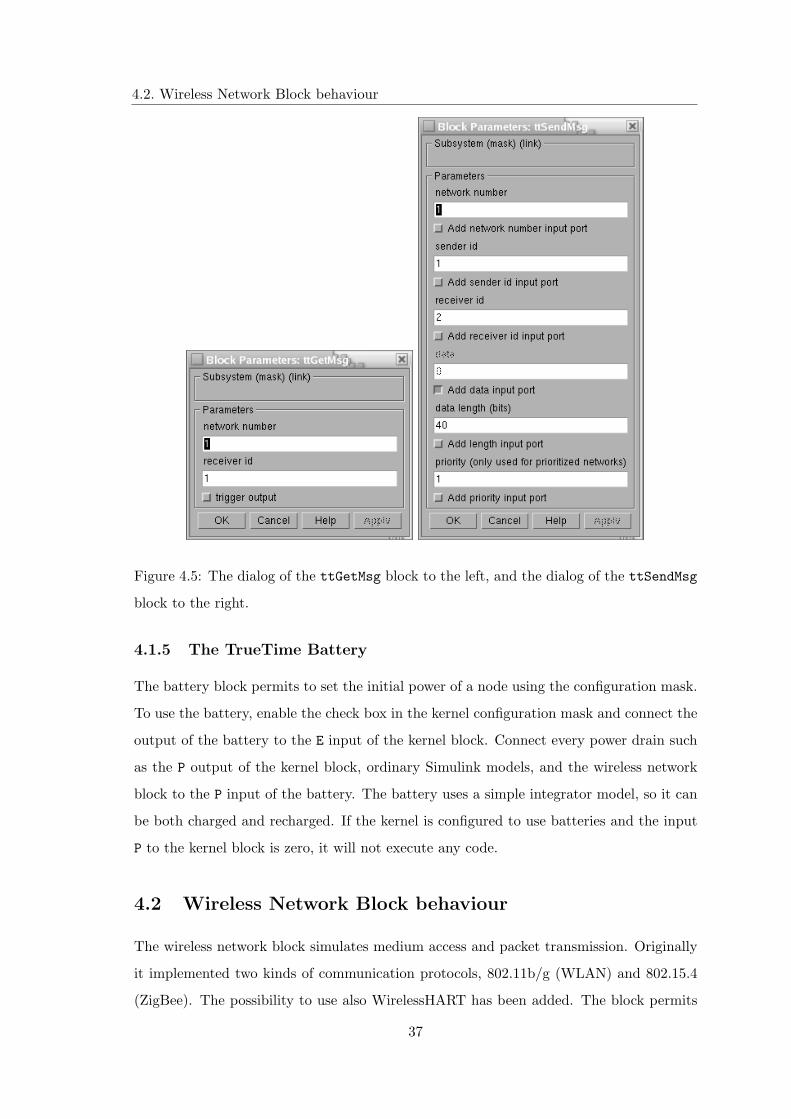
4.5 The dialog of the ttGetMsg block to the left, and the dialog of the ttSendMsg
block to the right. . . . . . . . . . . . . . . . . . . . . . . . . . . . . . . . . 37
4.6 Probability density function for a received symbol when using binary phase
shift keying and additive white Gaussian noise. . . . . . . . . . . . . . . . . 41
v
LIST OF FIGURES
5.1 The TrueTime wireless network block with the x,y,z coordinates inputs port that specifies
the true location of the nodes . . . . . . . . . . . . . . . . . . . . . . . . . . . . . 44
5.2 The wireless network block with the external noise input port. . . . . . . . 45
5.3 The average and the variance fields in the wireless network block mask . . . 46
5.4 The plot of the lost packets and the consequences in the control performance 47
5.5 The wireless network block with the output port for the packet lost signal . . . . . . . 47
5.6 Settings for the fixed packets lost option . . . . . . . . . . . . . . . . . . . . 48
5.7 The plot of the packets lost and the consequence in the control performance 49
5.8 The parameters setting in the WirelessHart mask . . . . . . . . . . . . . . . 50
5.9 MAC protocol location in TrueTime . . . . . . . . . . . . . . . . . . . . . . 50
5.10 MAC protocol location in a real environment . . . . . . . . . . . . . . . . . 51
6.1 Dead-time . . . . . . . . . . . . . . . . . . . . . . . . . . . . . . . . . . . . . 53
6.2 Jitter effect in event driven control. . . . . . . . . . . . . . . . . . . . . . . . 54
6.3 Jitter effect in time driven control. . . . . . . . . . . . . . . . . . . . . . . . 54
6.4 Delay caused by clock drift. . . . . . . . . . . . . . . . . . . . . . . . . . . . 55
6.5 Internal model control structure. . . . . . . . . . . . . . . . . . . . . . . . . 56
6.6 Standard control loop. . . . . . . . . . . . . . . . . . . . . . . . . . . . . . . 57
6.7 The IAE error changing the delay and the system time constant. . . . . . . 58
6.8 The IAE error changing the delay and the closed-loop time constant. . . . . 60
6.9 The PI controller. . . . . . . . . . . . . . . . . . . . . . . . . . . . . . . . . . 62
6.10 The PPI controller. . . . . . . . . . . . . . . . . . . . . . . . . . . . . . . . . 63
6.11 The Modified Smith Predictor. . . . . . . . . . . . . . . . . . . . . . . . . . 64
6.12 The Modified Smith Predictor when d is equal to zero. . . . . . . . . . . . . 65
6.13 The integral absolute error for the various methods considering a first order
system. . . . . . . . . . . . . . . . . . . . . . . . . . . . . . . . . . . . . . . 66
6.14 The integral absolute error for the various methods considering an integrating system. . . 67
6.15 AC800 typical scenario . . . . . . . . . . . . . . . . . . . . . . . . . . . . . . 68
6.16 Cascade loops . . . . . . . . . . . . . . . . . . . . . . . . . . . . . . . . . . . 69
6.17 A possible scenario. . . . . . . . . . . . . . . . . . . . . . . . . . . . . . . . . . 69
6.18 Representation of the simulated control system . . . . . . . . . . . . . . . . 71
6.19 Communication schedule . . . . . . . . . . . . . . . . . . . . . . . . . . . . . 71
6.20 WirelessHART parameters . . . . . . . . . . . . . . . . . . . . . . . . . . . . 72
vi

LIST OF FIGURES
6.21 The drift field in the controller kernel block . . . . . . . . . . . . . . . . . . 73
6.22 Reference tracking using the PI controller both with drift and without . . . 74
6.23 The PPI scheme . . . . . . . . . . . . . . . . . . . . . . . . . . . . . . . . . 74
6.24 Comparison of reference tracking between PI and PPI . . . . . . . . . . . . 75
6.25 IAE : PI and PPI controllers . . . . . . . . . . . . . . . . . . . . . . . . . . 76
6.26 Finite state machine: D=0 no delay, D=1 delay of 1 cycle . . . . . . . . . . . . . . . 77
6.27 Schedule of the tasks and detection of the delay . . . . . . . . . . . . . . . 77
6.28 Scheme of the detection of the delay due to the drift . . . . . . . . . . . . . 78
6.29 Detection of the delay due to the drift is one cycle late . . . . . . . . . . . . . . . . . 78
6.30 Detection of the delay due to the drift improvement . . . . . . . . . . . . . 79
6.31 Performance comparison between the hybrid controller, the PPI and the PI. . . . . . . 80
6.32 IAE comparison between the hybrid controller, the PPI and the PI. . . . . . . . . . . 80
6.33 Simulink model of the system with input disturbance . . . . . . . . . . . . . . . . . 81
6.34 System output with disturbance and drift . . . . . . . . . . . . . . . . . . . . . . . 81
6.35 IAE with disturbance and drift . . . . . . . . . . . . . . . . . . . . . . . . . . . . 82
6.36 System output with disturbance, drift and a square wave reference . . . . . 82
6.37 IAE with disturbance, drift and a square wave reference . . . . . . . . . . . 83
6.38 System output using PI control with drift and without. . . . . . . . . . . . 84
6.39 Integral Absolute Error using a PI control both with drift and without. . . 84
6.40 The modified Smith predictor for integrating process. . . . . . . . . . . . . . 85
6.41 Behaviour of the modified Smith predictor in presence of drift compared with the perfor-
mance of the PI controller. . . . . . . . . . . . . . . . . . . . . . . . . . . . . . . 86
6.42 Integral Absolute Error of the modified Smith predictor in presence of drift compared
with the performance of the PI controller. . . . . . . . . . . . . . . . . . . . . . . . 86
6.43 Behavior of the modified Smith predictor in presence of drift with F=λ. . . 87
6.44 The system output using the hybrid controller compared with a normal PI and the MSP. 88
6.45 IAE of the hybrid controller compared with a normal PI and the MSP. . . . . . . . . . 88
6.46 Behaviour of the hybrid controller in presence of input disturbance for different choice of F. 89
A.1 The TrueTime 1.5 block library. . . . . . . . . . . . . . . . . . . . . . . . . 93
B.1 The execution of user code is modeled by a sequence of segments executed
in order by the kernel. . . . . . . . . . . . . . . . . . . . . . . . . . . . . . . 95
vii
LIST OF FIGURES
B.2 Controllers represented using ordinary discrete Simulink blocks may be called from
within the code functions. The only requirement is that the blocks are discrete
with the sample time set to one. . . . . . . . . . . . . . . . . . . . . . . . . . . 97
C.1 Example: A control loop with 3 nodes. . . . . . . . . . . . . . . . . . . . . . 103
C.2 Example: Two control loops. . . . . . . . . . . . . . . . . . . . . . . . . . . 107
C.3 Example: Two control loops and shared slots. . . . . . . . . . . . . . . . . . 110
C.4 Example: Packets lost and prediction. . . . . . . . . . . . . . . . . . . . . . 112
viii
List of Tables
3.1 Example BOCntr Selection Sets . . . . . . . . . . . . . . . . . . . . . . . . . 25
3.2 Device Table . . . . . . . . . . . . . . . . . . . . . . . . . . . . . . . . . . . 28
B.1 Example of a P-controller code function written in Matlab code. . . . . . . 95
B.2 The C++ version of the code function in Listing B.1. . . . . . . . . . . . . 96
B.3 Simulink block diagrams are called from within code function using the TrueTime
function ttCallBlockSystem. . . . . . . . . . . . . . . . . . . . . . . . . . . . 97
B.4 Example of a TrueTime initialization script in the Matlab version. The kernel
is initialized using the function ttInitKernel, and a periodic task is created that
uses the P-controller code function from Listing B.1. The period of the controller
is passed to the initialization script as a parameter. . . . . . . . . . . . . . . . . 98
B.5 Template for writing initialization scripts in C++. The final script is actually a
complete Matlab S-function, since the included file, ttkernel.cpp, contains the
Simulink callback functions that implement the kernel. . . . . . . . . . . . . . . 99
B.6 Example of a TrueTime initialization script in the C++ version. Corresponds to
the Matlab version from Listing B.4. . . . . . . . . . . . . . . . . . . . . . . . . 101
C.1 Example of a TrueTime initialization script in the Matlab version. . . . . . . . . 104
C.2 Example of a sensor code. . . . . . . . . . . . . . . . . . . . . . . . . . . . 105
C.3 Example of transmissions schedule using different channels and multi-hop. 107
C.4 Example of transmissions schedule using shared slot. . . . . . . . . . . . . 108
D.1 Real-time primitives. . . . . . . . . . . . . . . . . . . . . . . . . . . . . . . . 114
D.2 Commands used to create, initialize TrueTime objects, to control the simulation
and used to set and get task attributes. . . . . . . . . . . . . . . . . . . . . . . 115
D.3 Real-time primitives. . . . . . . . . . . . . . . . . . . . . . . . . . . . . . . . 116
ix
Chapter 1
Introduction
Wireless technologies are becoming more and more important both in public and in indus-
trial environments. The aim of technique is to remove the constrictions if being attached
to expensive and messy cables. The advantages given by wireless technology are several.
First of all, it permits to carry the capability of wired networks to areas that cables can-
not reach. Considering industrial plants, wireless technologies can significantly facilitate
deployment and reconfiguration by eliminating the need for installing and maintaining
cabling, reducing both cost and time. However, the lack of maturity, the failure to provide
real-time performance and the lack of reliability metrics comparable to those of wired net-
works do not help the use of this technology in industrial environments. This thesis work
has been made at ABB Corporate Research in Sweden and is part of the SOCRADES
European project [22]. One of the main objectives of this project is to specify a new wire-
less communication architecture that provides the required reliability, safety, security and
real-time parameters for wireless sensor networks. The SOCRADES consortium is made
up of 15 partners from 6 European countries. It is led by the major European players
in the industrial automation sector (Schneider Electric, ABB, ARM, Boliden, FlexLink,
APS, SAP, Siemens, Ifak, Jaguar Cars Ltd.) and many European universities (Politecnico
di Milano, Loughborough University, TUT, KTH, LTU).
The aims of this thesis work are two. The first one is the implementation of a Wire-
lessHART network simulator. WirelessHART is a new wireless protocol that aims to
establish a new communication standard for process automation applications [4]. The
simulator has been written in C++ and interfaced with MATLAB through a S-function,
to have a friendly use of it. The possibility to work with this simulator has been added in
1
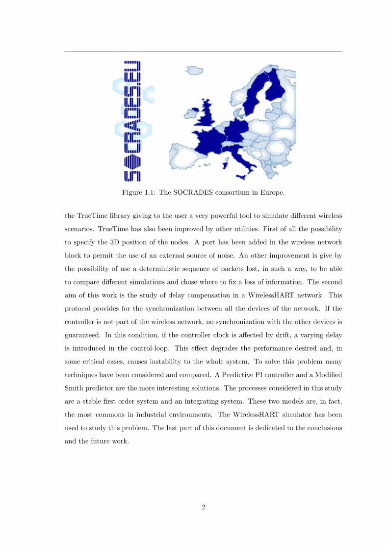
Figure 1.1: The SOCRADES consortium in Europe.
the TrueTime library giving to the user a very powerful tool to simulate different wireless
scenarios. TrueTime has also been improved by other utilities. First of all the possibility
to specify the 3D position of the nodes. A port has been added in the wireless network
block to permit the use of an external source of noise. An other improvement is give by
the possibility of use a deterministic sequence of packets lost, in such a way, to be able
to compare different simulations and chose where to fix a loss of information. The second
aim of this work is the study of delay compensation in a WirelessHART network. This
protocol provides for the synchronization between all the devices of the network. If the
controller is not part of the wireless network, no synchronization with the other devices is
guaranteed. In this condition, if the controller clock is affected by drift, a varying delay
is introduced in the control-loop. This effect degrades the performance desired and, in
some critical cases, causes instability to the whole system. To solve this problem many
techniques have been considered and compared. A Predictive PI controller and a Modified
Smith predictor are the more interesting solutions. The processes considered in this study
are a stable first order system and an integrating system. These two models are, in fact,
the most commons in industrial environments. The WirelessHART simulator has been
used to study this problem. The last part of this document is dedicated to the conclusions
and the future work.
2
1.1. Outline of the thesis
1.1 Outline of the thesis
The contents of the thesis are as follows:
1.1.1 Chapter 2: Network theory
Industrial communications constitute, today, a fundamental topic for all kind of automa-
tion. The aim of this chapter is to introduce the basis of the network theory in order
to create a background for the understanding of the whole thesis. In this chapter are
introduced the OSI model, some different MAC protocol and the IEEE 802 standards.
1.1.2 Chapter 3: WirelessHART
In this chapter the WirelessHART protocol will be described. First, a general introduction
to the protocol is given. Later the structure of the MAC is deeply explained, and a more
exhaustive description of the communication protocol is given. The chapter is concluded
with the description of the implementation of the WirelessHART MAC protocol in a C++
code.
1.1.3 Chapter 4: Introduction to TrueTime
This chapter describes the use of the original Matlab/Simulink-based simulator True-
Time, which facilitates co-simulation of controller task execution in real-time kernels,
network transmissions (using wired or wireless networks), and continuous plant dynam-
ics. A detailed description of the six blocks that compose the library (the kernel block,
the network block, the wireless network block, the battery block the ttSendMsg and the
ttGetMsg blocks) is given. The same tool has been modified to permit the use of the
WirelessHART protocol and some more utilities have been added.
1.1.4 Chapter 5: New functions in the wireless network block
This chapter contains some new utilities implemented to improve the behavior and the
useability of the wireless network block of TrueTime. The 3D position of a node is the first
improvement. After that are described the use and the implementation of the external
source of noise, the time correlation function and the fixed sequence of packets lost. The
last section of this chapter is dedicated to the configuration of WirelessHART in the mask
of the wireless network block.
3
1.1. Outline of the thesis
1.1.5 Chapter 6: Delay compensation
This chapter introduces how the most common systems in industry can be affected by
delay and some possible solutions to overcome this problem. First of all, the problem of
delay in a control loop is introduced and its possible sources. After that, it investigates
how the performance of a control loop could be influenced by a delay considering some
typical industrial systems. Possible solutions that the controller can adopt to improve its
performance are investigated. A brief description of the controller AC800M is also given.
The last section deals with the problem of delay due to the clock drift using a controllers
like the AC800M in a WirelessHART scenario and proposes some solutions considering
different processes.
1.1.6 Chapter 7: Conclusions
The last chapter presents the conclusions of this thesis work. Future work is also discussed.
4
Chapter 2
Network theory
Industrial communications constitute, today, a fundamental topic for all kind of automa-
tion. The aim of this chapter is to introduce the basis of the network theory in order
to create a background for the understanding of the whole thesis. The first section is
an introduction to the main structure of the Open System Interconnection model (OSI).
In section 2.2 a description of the Medium Access Protocol (MAC) has been given. The
IEEE 802 standard is described in section 2.3. In the last section a brief overview of the
major part of the actual wireless protocols is presented.
2.1 The Open System Interconnection model (OSI)
The OSI model [21] is a conceptual framework of standards for communication in the
network. It has been developed by the International Standards Organization (ISO) in
1984 and it is now considered the primary architectural model for network communication.
Most of the network protocols used today have a structure based on the OSI model.
2.1.1 The OSI basic structure
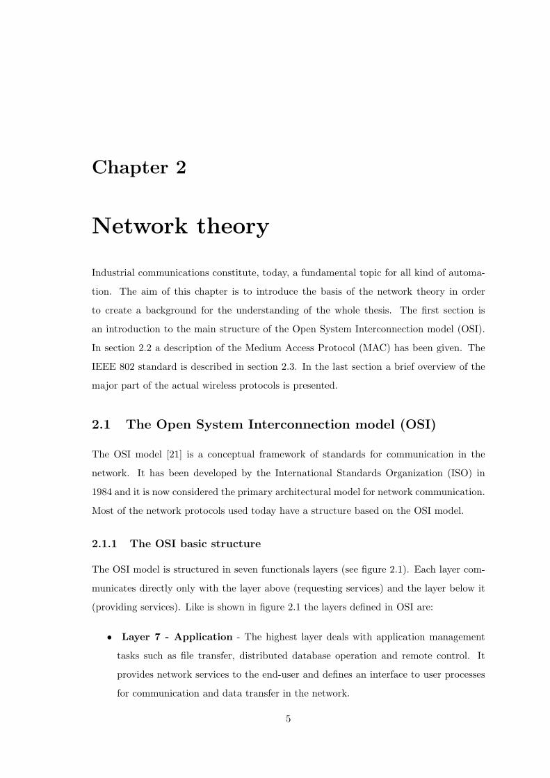
The OSI model is structured in seven functionals layers (see figure 2.1). Each layer com-
municates directly only with the layer above (requesting services) and the layer below it
(providing services). Like is shown in figure 2.1 the layers defined in OSI are:
• Layer 7 - Application - The highest layer deals with application management
tasks such as file transfer, distributed database operation and remote control. It
provides network services to the end-user and defines an interface to user processes
for communication and data transfer in the network.
5
2.1. The Open System Interconnection model (OSI)
Figure 2.1: The Open System Interconnection (OSI) model
• Layer 6 : Presentation - This layer provides data encoding and conversion. It
converts user local representation of data to its canonical form and vice versa.
• Layer 5 : Session - The layer defines the format of the data sent over the con-
nection. It enhances the transport layer by adding services to support full session
between different nodes. An example is the network login in a remote computer.
• Layer 4 : Transport - End to end communication control. This layer is the
interface between the application software that request data communication and the
physical network represented by the first three layers. The transport layer has the
responsibility of verifing that the data is transmitted and received correctly from
a node of the network to another and that the data is available for application
programs.
• Layer 3 : Network - This layer sets up a complete communication path and
oversees that messages travel all the way from the sources to the destination node.
When a packet has to travel from one network to another to get to its destination,
many problems can arise. The addressing used by the second network may be
different from the first one. The second one may not accept the packet at all because
it is too large. The protocols may differ, and so on. It is up to the network layer to
overcome all these problems to allow heterogeneous networks to be interconnected.
• Layer 2 : Data Link - This level provides for the verification that bit sequences
6
2.1. The Open System Interconnection model (OSI)
are passed correctly between two nodes. If errors occur, for example because of
disturbances, the retransmission of a corrupted bit sequence may be request at the
data link layer. As a result the data link layer present to highest layers an error-free
data link between the nodes.
• Layer 1 : Physical - This is the electrical, optical or radio communication medium
with the related interfaces to the communicating network nodes. All details about
transmission medium, signal levels, frequencies are handled at this level. The phys-
ical layer is the only real connection between two nodes.
The requesting layer passes parameters and data to the layer below it and waits for an
answer. Modules that are located at the same layer and at different points in the communi-
cation network (i.e. running on different nodes) are called peers. The peers communicate
via protocols that define message formats and the rules for data exchange. Following the
OSI rules only peers are allowed to communicate with each other. Two peer entities are
connected by a virtual link that appears, to the peers, like a real communication channel.
Only at the first layer the virtual and the physical connection are the same. The peers
exchange data according to a protocol specified for their level. There is not direct link,
real or virtual, between modules of the same node, at a distance of more than one layer
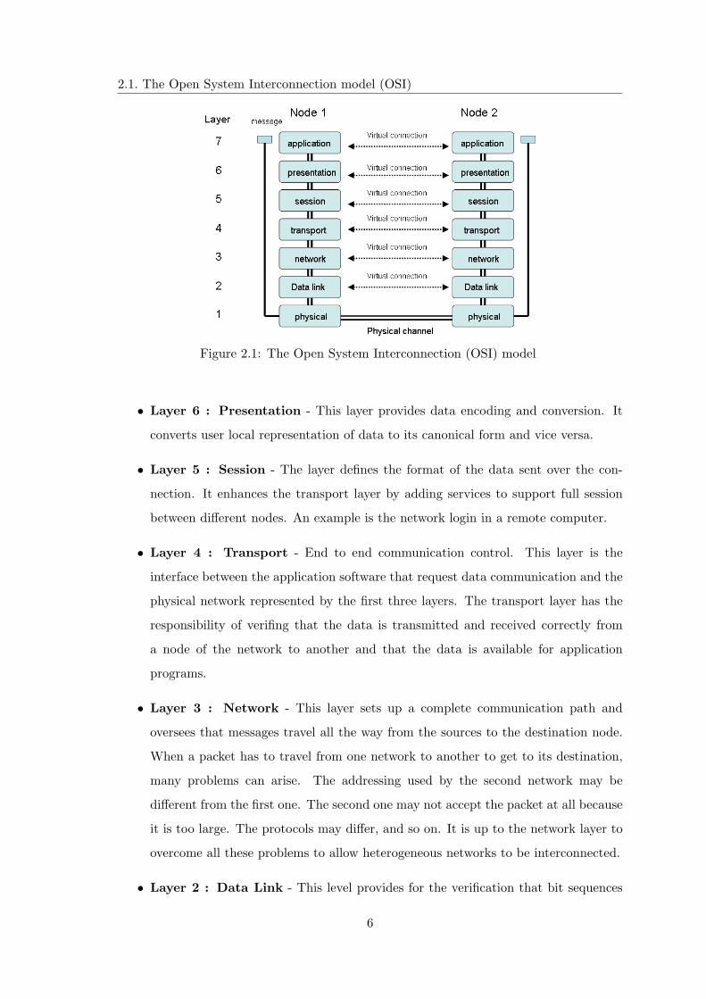
from each other. Each layer has its own communication protocol and adds therefore the
related data to the original message (see figure 2.2).
Figure 2.2: The amount of data in the Open System Interconnection (OSI) model
The result is an incremental amount of data in the message that has to be sent.
7
2.2. The Medium Access Control (MAC) protocol
2.2 The Medium Access Control (MAC) protocol
The Medium Access Control (MAC) data communication protocol belongs to a sub-layer
of the Data Link layer specified in the OSI model. The protocol provides addressing and
channel access control mechanism. In fact, in any broadcast channel, the key issue is how
to determine who gets to use the medium when there is competition for it. Many MAC
protocols for solving the problem are known. The principals are:
• ALOHA
• Carrier Sense Multiple Access Protocols (CSMA)
– CSMA/CD - for wired networks (i.e. Ethernet)
– CSMA/CA - for wireless networks (i.e. Wireless LAN)
• Time Division Multiple Access (TDMA)
• Token Bus
• Token Ring
2.2.1 ALOHA
This is an old protocol, one of the first that proposed the use of random access radio
communications. The ALOHA protocol [18] was born in the 70s to provide Wireless links
between the universities and some research-institutes spread around the Hawaiian islands.
The protocol used is really simple. It consists in just sending when the data is ready. If
a collision occurs, then it detects errored frames and retransmits the data with a random
time delay. The result of this simple protocol is the possibility to have a decentralized
network that works well for low loads. In 1972, Roberts published a method for doubling
the capacity of an ALOHA system [19]. His proposal was to divide time into discrete
intervals, each interval corresponding to one frame. This approach requires the users to
agree on slot boundaries. One way to achieve synchronization would be to have one special
station that emits a beep at the start of each interval, like a clock. The Roberts’ method
has come to be known as slotted ALOHA.
8
2.2. The Medium Access Control (MAC) protocol
2.2.2 Carrier Sense Multiple Access Protocols (CSMA)
Carrier Sense Multiple Access Protocols (CSMA) [19] are probabilistic MAC protocols in
which a node verifies the absence of other traffic before transmitting on a shared physical
medium. The nodes listen if the channel is idle (carrier sense ) before transmitting. If
the channel is in use, the devices wait a random amount of time before retrying. Multiple
access (MA) indicates that many devices can connect and share the same network. All
devices have equal access to use the network when it is idle. Even though devices attempt
to sense whether the network is in use, there is a good chance that two nodes will attempt
to access it at the same time. In this case a collision occurs. There are two main protocols
that differs in the way the collisions are treated :
• CSMA/CD - (i.e. Ethernet)
• CSMA/CA - (i.e. Wireless LAN)
Carrier Sense Multiple Access Protocols / Collision Detection (CSMA/CD)
Carrier Sense Multiple Access Protocols with collision detection defines what happens
when two devices sense the channel to be idle and begin transmitting simultaneously. A
collision occurs, and both devices stop transmission, wait for a random amount of time
(back-off time), then retransmit. Collisions can be detected by looking at the power or
pulse width of the received signal and comparing it to the transmitted signal.
Carrier Sense Multiple Access Protocols / Collision Avoidance (CSMA/CA)
In the collision avoidance (CA) [17] technique when a node has to transmit, it first checks
the medium to ensure no other node is transmitting. If the channel is idle, it then transmits
the packet. Otherwise, it chooses a random ”back-off factor” which determines the amount
of time the node must wait until it is allowed to transmit its packet. During periods in
which the channel is idle, the transmitting node decrements its back-off counter (when the
channel is busy it does not decrement its back-off counter). When the back-off counter
reaches zero, the node transmits the packet. There is no possibility to detect a collision but
if a message is not acknowledged, the transmitting node assumes a collision has occurred
and retransmits. The collision avoidance permits to reduce the probability that a collision
occurs but it is not possible to detect when it happens. In fact, collision detection cannot
be used for the radio frequency transmissions. The reason for this is that, when a node
9
2.2. The Medium Access Control (MAC) protocol
is transmitting, it cannot hear any other node in the system which may be transmitting,
since its own signal will drown out any others arriving at the node.
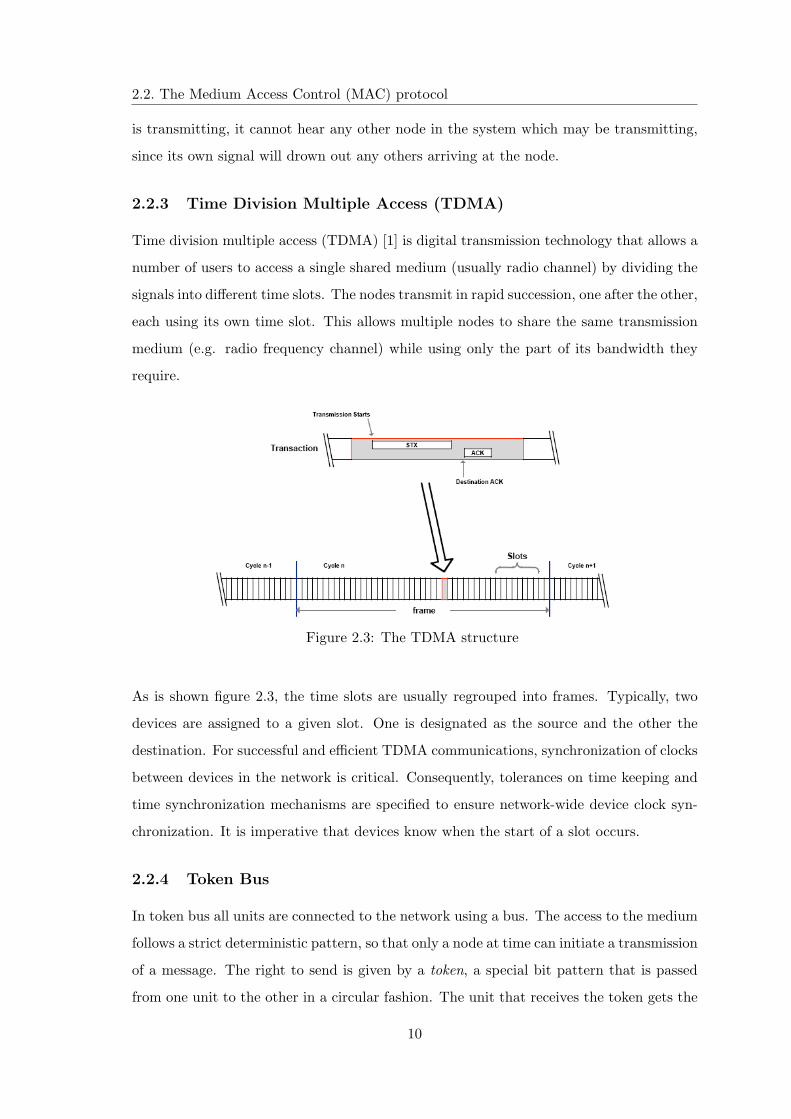
2.2.3 Time Division Multiple Access (TDMA)
Time division multiple access (TDMA) [1] is digital transmission technology that allows a
number of users to access a single shared medium (usually radio channel) by dividing the
signals into different time slots. The nodes transmit in rapid succession, one after the other,
each using its own time slot. This allows multiple nodes to share the same transmission
medium (e.g. radio frequency channel) while using only the part of its bandwidth they
require.
Figure 2.3: The TDMA structure
As is shown figure 2.3, the time slots are usually regrouped into frames. Typically, two
devices are assigned to a given slot. One is designated as the source and the other the
destination. For successful and efficient TDMA communications, synchronization of clocks
between devices in the network is critical. Consequently, tolerances on time keeping and
time synchronization mechanisms are specified to ensure network-wide device clock syn-
chronization. It is imperative that devices know when the start of a slot occurs.
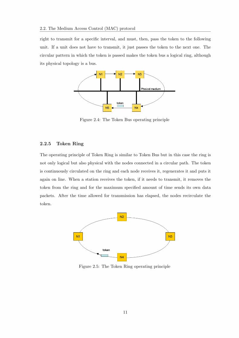
2.2.4 Token Bus
In token bus all units are connected to the network using a bus. The access to the medium
follows a strict deterministic pattern, so that only a node at time can initiate a transmission
of a message. The right to send is given by a token, a special bit pattern that is passed
from one unit to the other in a circular fashion. The unit that receives the token gets the
10
2.2. The Medium Access Control (MAC) protocol
right to transmit for a specific interval, and must, then, pass the token to the following
unit. If a unit does not have to transmit, it just passes the token to the next one. The
circular pattern in which the token is passed makes the token bus a logical ring, although
its physical topology is a bus.
Figure 2.4: The Token Bus operating principle
2.2.5 Token Ring
The operating principle of Token Ring is similar to Token Bus but in this case the ring is
not only logical but also physical with the nodes connected in a circular path. The token
is continuously circulated on the ring and each node receives it, regenerates it and puts it
again on line. When a station receives the token, if it needs to transmit, it removes the
token from the ring and for the maximum specified amount of time sends its own data
packets. After the time allowed for transmission has elapsed, the nodes recirculate the
token.
Figure 2.5: The Token Ring operating principle
11
2.3. The IEEE 802 standards
2.3 The IEEE 802 standards
In this section the family IEEE 802 and some related protocols, used in wireless communi-
cation, are briefly described. The standards here considered are chosen for their diffusion
in both industrial and public environments for implementing wireless networks. The very
extensive 802 group of IEEE standards is concerned with Local Area Networks (LANs)
and the development of many of these standards have had a major impact [20].
2.3.1 Bluetooth/IEEE 802.15.1
Bluetooth Wireless TechnologyTM is a lowcost/short-range (up to 10m) wireless network-
ing method for personal, office and industrial environments [17]. The name originates
from a Danish King, Harald Blatand, who is considered to have succeeded in uniting the
Scandinavian people in the 10th century AD. The aim of this Standard was, instead, to
unite personal computing devices. A frequency-hopping spread-spectrum technique is used
with 1600 hops/s at 79 frequencies. The frequency-sequence is selected in a pseudo-random
manner. All Bluetooth devices share the same frequency space, and the band may be used
concurrently by other ISM devices. There are two main classes of frequency-hopper; those
that have many bits per hop and those that have many hops per bit. Bluetooth uses the
first class. The Bluetooth standard allows three transmit-power classes: 1mW, 2.5mW
and 100mW. Most applications are in the first two classes, which provide ranges of 100mm
to 10m respectively. It is easy to notice that, Bluetooth has a low consumption but is able
to work only in short range. The maximum data rate for Bluetooth is 1 Mbps (3 Mbps
v2.1), using Gaussian binary frequency shift keying (FSK). It makes Bluetooth inadequate
for some consumer applications such as MPEG2 video data stream for a high-definition
TV display and for Real-time computer graphics. It supports maximum 7 slave devices
controlled by a master. In order to establish a net of devices ( piconet), the master
transmits ’enquiry messages’ at 1.28 second intervals in order to locate Bluetooth devices
within range. This is followed by ’invitations to join the piconet’ addressed to the specific
devices within range that the master wishes to have in the net. The master allocates a
member-address to each of the active slaves, and controls their transmissions. The clock
of the master provides the time synchronization of the whole piconet. The master always
transmits in ’even-numbered’ time-slots and the slaves transmit in ’odd-numbered’ time-
slots in accordance with permission given by the master. Each channel is divided into
12
2.3. The IEEE 802 standards
time slots of 625 µs. The master switches from slave to slave in a round-robin fashion.
The 802.15 working group is developing a family of ’Wireless Personal Area Networks’
(WPANs) for up to 55Mb/s data-rate, and Bluetooth has been accepted as one of these.
In March 2002, Bluetooth was ratified by IEEE for 802.15.1.
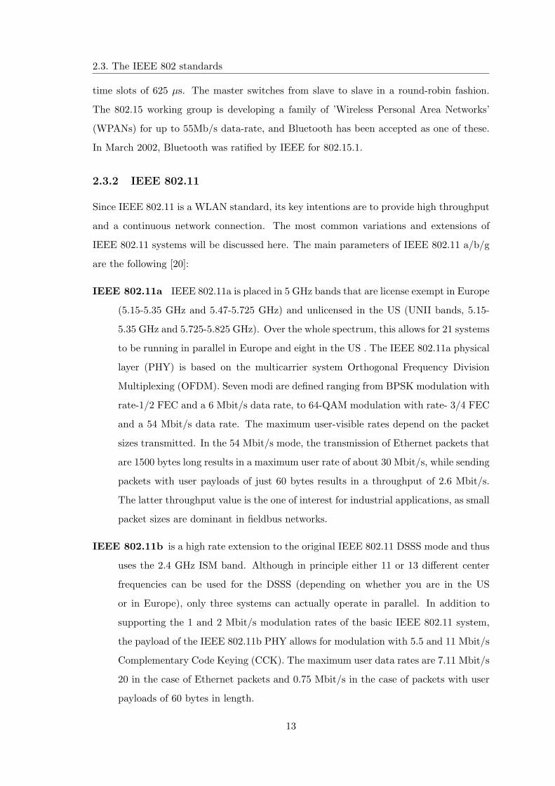
2.3.2 IEEE 802.11
Since IEEE 802.11 is a WLAN standard, its key intentions are to provide high throughput
and a continuous network connection. The most common variations and extensions of
IEEE 802.11 systems will be discussed here. The main parameters of IEEE 802.11 a/b/g
are the following [20]:
IEEE 802.11a IEEE 802.11a is placed in 5 GHz bands that are license exempt in Europe
(5.15-5.35 GHz and 5.47-5.725 GHz) and unlicensed in the US (UNII bands, 5.15-
5.35 GHz and 5.725-5.825 GHz). Over the whole spectrum, this allows for 21 systems
to be running in parallel in Europe and eight in the US . The IEEE 802.11a physical
layer (PHY) is based on the multicarrier system Orthogonal Frequency Division
Multiplexing (OFDM). Seven modi are defined ranging from BPSK modulation with
rate-1/2 FEC and a 6 Mbit/s data rate, to 64-QAM modulation with rate- 3/4 FEC
and a 54 Mbit/s data rate. The maximum user-visible rates depend on the packet
sizes transmitted. In the 54 Mbit/s mode, the transmission of Ethernet packets that
are 1500 bytes long results in a maximum user rate of about 30 Mbit/s, while sending
packets with user payloads of just 60 bytes results in a throughput of 2.6 Mbit/s.
The latter throughput value is the one of interest for industrial applications, as small
packet sizes are dominant in fieldbus networks.
IEEE 802.11b is a high rate extension to the original IEEE 802.11 DSSS mode and thus
uses the 2.4 GHz ISM band. Although in principle either 11 or 13 different center
frequencies can be used for the DSSS (depending on whether you are in the US
or in Europe), only three systems can actually operate in parallel. In addition to
supporting the 1 and 2 Mbit/s modulation rates of the basic IEEE 802.11 system,
the payload of the IEEE 802.11b PHY allows for modulation with 5.5 and 11 Mbit/s
Complementary Code Keying (CCK). The maximum user data rates are 7.11 Mbit/s
20 in the case of Ethernet packets and 0.75 Mbit/s in the case of packets with user
payloads of 60 bytes in length.
13
2.3. The IEEE 802 standards
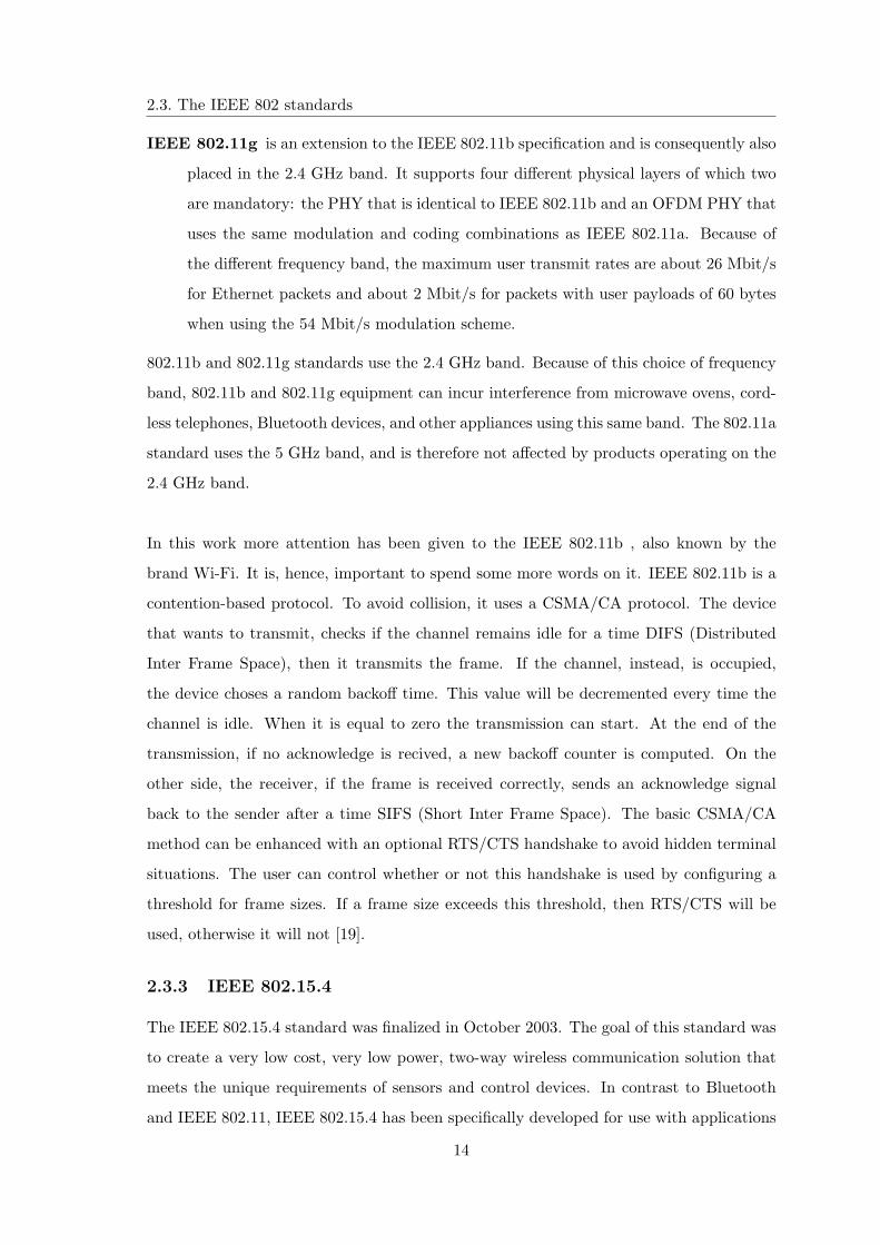
IEEE 802.11g is an extension to the IEEE 802.11b specification and is consequently also
placed in the 2.4 GHz band. It supports four different physical layers of which two
are mandatory: the PHY that is identical to IEEE 802.11b and an OFDM PHY that
uses the same modulation and coding combinations as IEEE 802.11a. Because of
the different frequency band, the maximum user transmit rates are about 26 Mbit/s
for Ethernet packets and about 2 Mbit/s for packets with user payloads of 60 bytes
when using the 54 Mbit/s modulation scheme.
802.11b and 802.11g standards use the 2.4 GHz band. Because of this choice of frequency
band, 802.11b and 802.11g equipment can incur interference from microwave ovens, cord-
less telephones, Bluetooth devices, and other appliances using this same band. The 802.11a
standard uses the 5 GHz band, and is therefore not affected by products operating on the
2.4 GHz band.
In this work more attention has been given to the IEEE 802.11b , also known by the
brand Wi-Fi. It is, hence, important to spend some more words on it. IEEE 802.11b is a
contention-based protocol. To avoid collision, it uses a CSMA/CA protocol. The device
that wants to transmit, checks if the channel remains idle for a time DIFS (Distributed
Inter Frame Space), then it transmits the frame. If the channel, instead, is occupied,
the device choses a random backoff time. This value will be decremented every time the
channel is idle. When it is equal to zero the transmission can start. At the end of the
transmission, if no acknowledge is recived, a new backoff counter is computed. On the
other side, the receiver, if the frame is received correctly, sends an acknowledge signal
back to the sender after a time SIFS (Short Inter Frame Space). The basic CSMA/CA
method can be enhanced with an optional RTS/CTS handshake to avoid hidden terminal
situations. The user can control whether or not this handshake is used by configuring a
threshold for frame sizes. If a frame size exceeds this threshold, then RTS/CTS will be
used, otherwise it will not [19].
2.3.3 IEEE 802.15.4
The IEEE 802.15.4 standard was finalized in October 2003. The goal of this standard was
to create a very low cost, very low power, two-way wireless communication solution that
meets the unique requirements of sensors and control devices. In contrast to Bluetooth
and IEEE 802.11, IEEE 802.15.4 has been specifically developed for use with applications
14
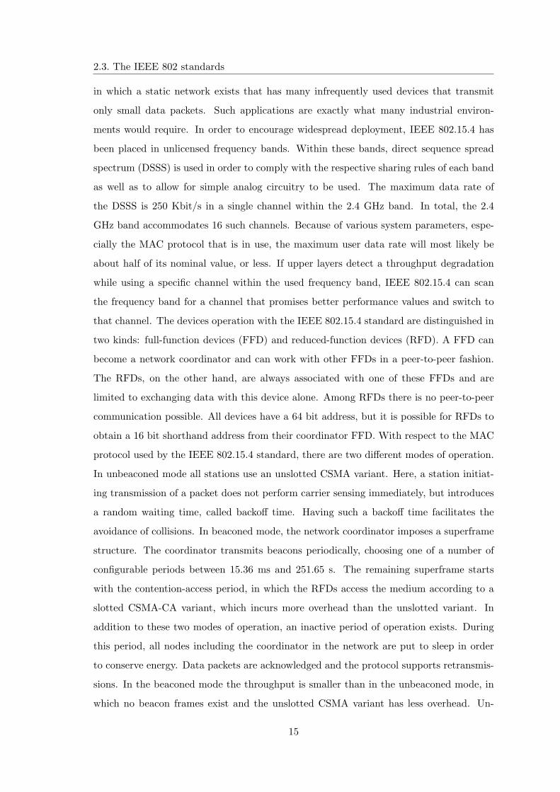
2.3. The IEEE 802 standards
in which a static network exists that has many infrequently used devices that transmit
only small data packets. Such applications are exactly what many industrial environ-
ments would require. In order to encourage widespread deployment, IEEE 802.15.4 has
been placed in unlicensed frequency bands. Within these bands, direct sequence spread
spectrum (DSSS) is used in order to comply with the respective sharing rules of each band
as well as to allow for simple analog circuitry to be used. The maximum data rate of
the DSSS is 250 Kbit/s in a single channel within the 2.4 GHz band. In total, the 2.4
GHz band accommodates 16 such channels. Because of various system parameters, espe-
cially the MAC protocol that is in use, the maximum user data rate will most likely be
about half of its nominal value, or less. If upper layers detect a throughput degradation
while using a specific channel within the used frequency band, IEEE 802.15.4 can scan
the frequency band for a channel that promises better performance values and switch to
that channel. The devices operation with the IEEE 802.15.4 standard are distinguished in
two kinds: full-function devices (FFD) and reduced-function devices (RFD). A FFD can
become a network coordinator and can work with other FFDs in a peer-to-peer fashion.
The RFDs, on the other hand, are always associated with one of these FFDs and are
limited to exchanging data with this device alone. Among RFDs there is no peer-to-peer
communication possible. All devices have a 64 bit address, but it is possible for RFDs to
obtain a 16 bit shorthand address from their coordinator FFD. With respect to the MAC
protocol used by the IEEE 802.15.4 standard, there are two different modes of operation.
In unbeaconed mode all stations use an unslotted CSMA variant. Here, a station initiat-
ing transmission of a packet does not perform carrier sensing immediately, but introduces
a random waiting time, called backoff time. Having such a backoff time facilitates the
avoidance of collisions. In beaconed mode, the network coordinator imposes a superframe
structure. The coordinator transmits beacons periodically, choosing one of a number of
configurable periods between 15.36 ms and 251.65 s. The remaining superframe starts
with the contention-access period, in which the RFDs access the medium according to a
slotted CSMA-CA variant, which incurs more overhead than the unslotted variant. In
addition to these two modes of operation, an inactive period of operation exists. During
this period, all nodes including the coordinator in the network are put to sleep in order
to conserve energy. Data packets are acknowledged and the protocol supports retransmis-
sions. In the beaconed mode the throughput is smaller than in the unbeaconed mode, in
which no beacon frames exist and the unslotted CSMA variant has less overhead. Un-
15
2.3. The IEEE 802 standards
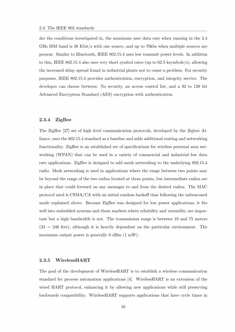
der the conditions investigated in, the maximum user data rate when running in the 2.4
GHz ISM band is 38 Kbit/s with one source, and up to 70kbs when multiple sources are
present. Similar to Bluetooth, IEEE 802.15.4 uses low transmit power levels. In addition
to this, IEEE 802.15.4 also uses very short symbol rates (up to 62.5 ksymbols/s), allowing
the increased delay spread found in industrial plants not to cause a problem. For security
purposes, IEEE 802.15.4 provides authentication, encryption, and integrity service. The
developer can choose between: No security, an access control list, and a 32 to 128 bit
Advanced Encryption Standard (AES) encryption with authentication.
2.3.4 ZigBee
The ZigBee [27] set of high level communication protocols, developed by the Zigbee Al-
liance, uses the 802.15.4 standard as a baseline and adds additional routing and networking
functionality. ZigBee is an established set of specifications for wireless personal area net-
working (WPAN) that can be used in a variety of commercial and industrial low data
rate applications. ZigBee is designed to add mesh networking to the underlying 802.15.4
radio. Mesh networking is used in applications where the range between two points may
be beyond the range of the two radios located at those points, but intermediate radios are
in place that could forward on any messages to and from the desired radios. The MAC
protocol used is CSMA/CA with an initial random backoff time following the unbeaconed
mode explained above. Because ZigBee was designed for low power applications, it fits
well into embedded systems and those markets where reliability and versatility are impor-
tant but a high bandwidth is not. The transmission range is between 10 and 75 meters
(33 ∼ 246 feet), although it is heavily dependent on the particular environment. The
maximum output power is generally 0 dBm (1 mW).
2.3.5 WirelessHART
The goal of the development of WirelessHART is to establish a wireless communication
standard for process automation applications [4]. WirelessHART is an extension of the
wired HART protocol, enhancing it by allowing new applications while still preserving
backwards compatibility. WirelessHART supports applications that have cycle times in
16
2.3. The IEEE 802 standards
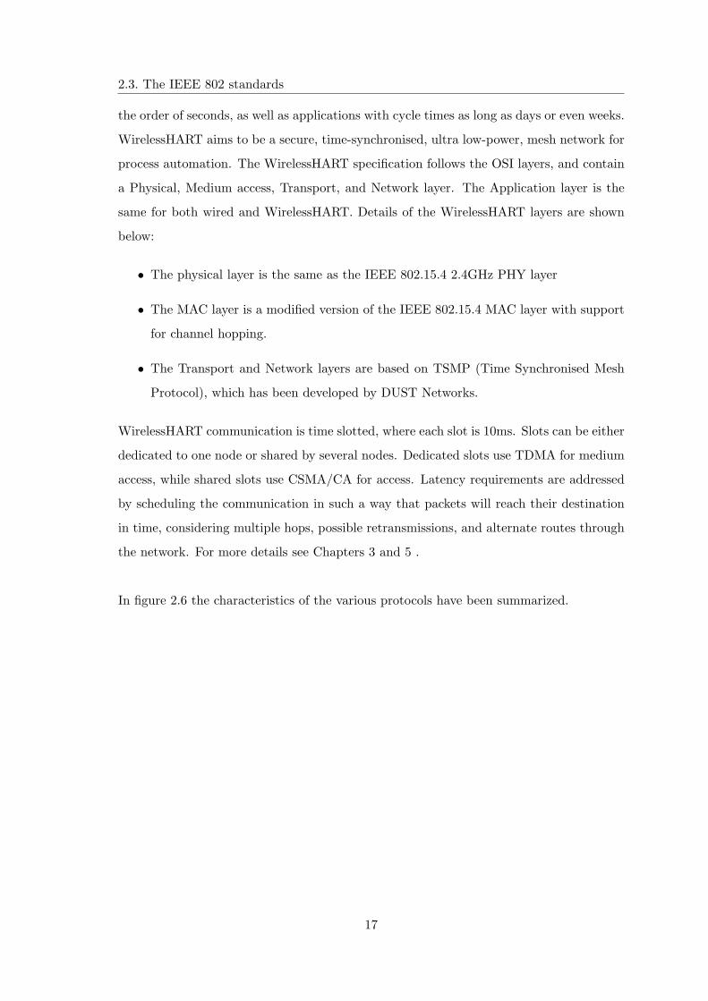
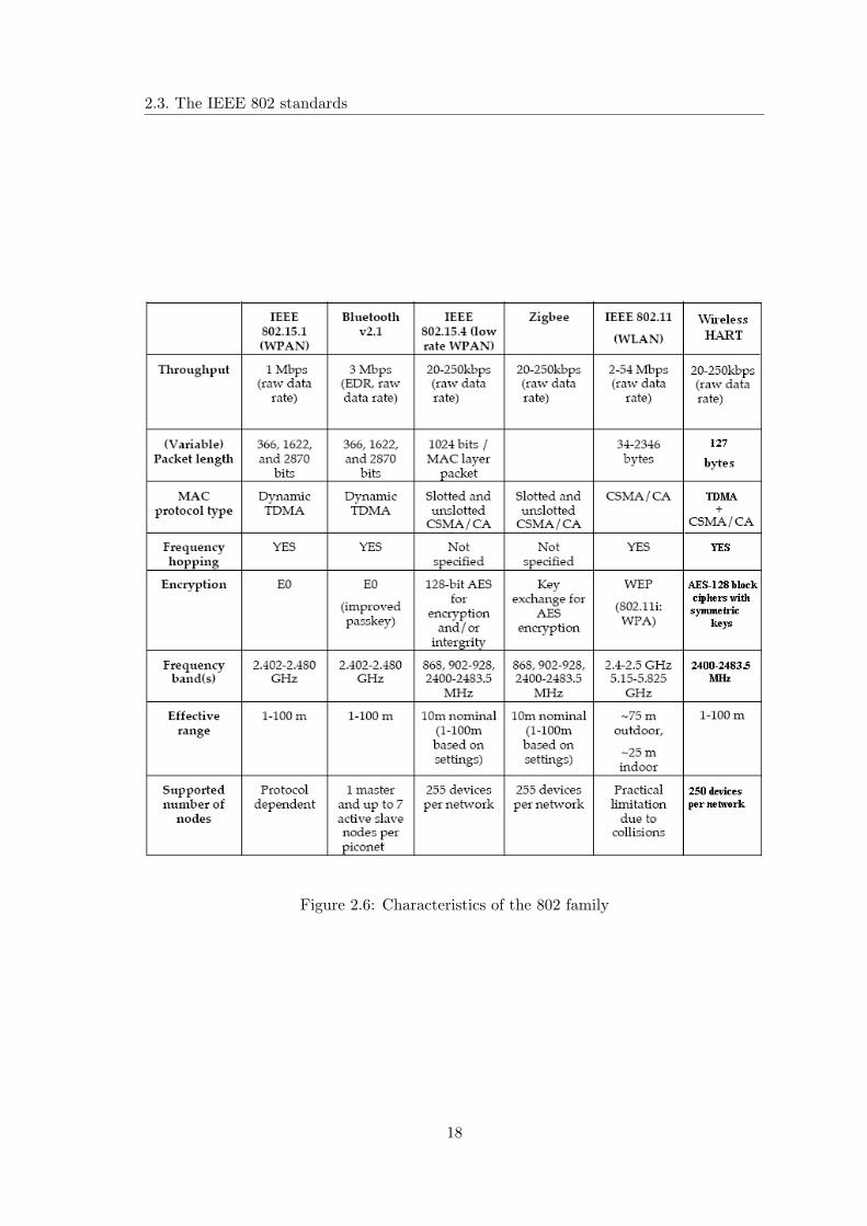
the order of seconds, as well as applications with cycle times as long as days or even weeks.
WirelessHART aims to be a secure, time-synchronised, ultra low-power, mesh network for
process automation. The WirelessHART specification follows the OSI layers, and contain
a Physical, Medium access, Transport, and Network layer. The Application layer is the
same for both wired and WirelessHART. Details of the WirelessHART layers are shown
below:
• The physical layer is the same as the IEEE 802.15.4 2.4GHz PHY layer
• The MAC layer is a modified version of the IEEE 802.15.4 MAC layer with support
for channel hopping.
• The Transport and Network layers are based on TSMP (Time Synchronised Mesh
Protocol), which has been developed by DUST Networks.
WirelessHART communication is time slotted, where each slot is 10ms. Slots can be either
dedicated to one node or shared by several nodes. Dedicated slots use TDMA for medium
access, while shared slots use CSMA/CA for access. Latency requirements are addressed
by scheduling the communication in such a way that packets will reach their destination
in time, considering multiple hops, possible retransmissions, and alternate routes through
the network. For more details see Chapters 3 and 5 .
In figure 2.6 the characteristics of the various protocols have been summarized.
17
2.3. The IEEE 802 standards
Figure 2.6: Characteristics of the 802 family
18
Chapter 3
WirelessHART
3.1 Introduction
In this chapter the WirelessHART protocol [1] will be described. The first section 3.2 is
a general introduction to the protocol with the main information and the technical char-
acteristics of WirelessHART. In section 3.3 the structure of the MAC is deeply explained,
and a more exhaustive description of the communication protocol is given. The last section
describes the code implementation of the ttMAC function.
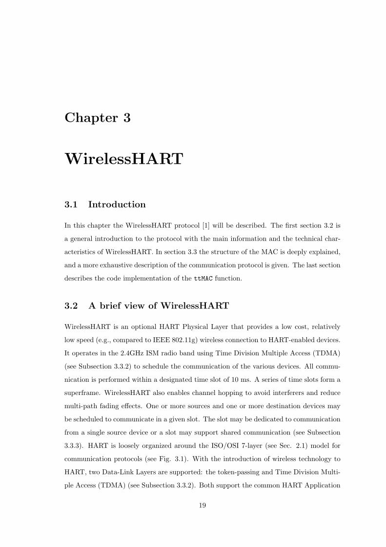
3.2 A brief view of WirelessHART
WirelessHART is an optional HART Physical Layer that provides a low cost, relatively
low speed (e.g., compared to IEEE 802.11g) wireless connection to HART-enabled devices.
It operates in the 2.4GHz ISM radio band using Time Division Multiple Access (TDMA)
(see Subsection 3.3.2) to schedule the communication of the various devices. All commu-
nication is performed within a designated time slot of 10 ms. A series of time slots form a
superframe. WirelessHART also enables channel hopping to avoid interferers and reduce
multi-path fading effects. One or more sources and one or more destination devices may
be scheduled to communicate in a given slot. The slot may be dedicated to communication
from a single source device or a slot may support shared communication (see Subsection
3.3.3). HART is loosely organized around the ISO/OSI 7-layer (see Sec. 2.1) model for
communication protocols (see Fig. 3.1). With the introduction of wireless technology to
HART, two Data-Link Layers are supported: the token-passing and Time Division Multi-
ple Access (TDMA) (see Subsection 3.3.2). Both support the common HART Application
19
3.2. A brief view of WirelessHART
Layer.
Figure 3.1: HART OSI 7-Layer Model [1].
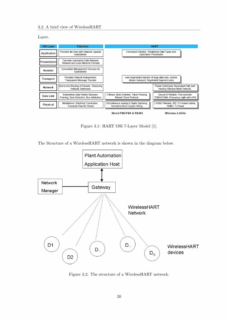
The Structure of a WirelessHART network is shown in the diagram below.
Figure 3.2: The structure of a WirelessHART network.
20
3.3. MAC Protocol Description
All communications of the WirelessHART Network pass through the gateway. Conse-
quently, the gateway must route packets to the specified destination (network Device,
host application, or network manager). The gateway uses standard HART commands to
communicate with network devices and host applications. The plant automation network
could be a TCP-based network, a remote IO system, or a bus such as PROFIBUS DP. The
Network Manager creates an initial superframe and configures the Gateway. A detailed
description of the components of a wirelessHART network is given in [2] and [3].
The MAC rules ensuring that transmissions by devices occur in an orderly fashion. In
other words, the protocol specifies when a device is allowed to transmit a message.
3.3 MAC Protocol Description
The main tasks of the MAC (Medium Access Control) protocol are:
• slot synchronization;
• identification of devices that need to access the medium;
• propagation of messages received from the Network Layer;
• to listen for packets being propagated from neighbors
The Medium Access Control (MAC) sub-layer is, hence, responsible for propagating Data-
Link packets (DLPDUs, see Subsection 3.3.1) across a link. To permit this, the device
includes:
• Tables of neighbors, superframes, links, and graphs that configure the communica-
tion between the device and its neighbors (see Subsection 3.4.2). These tables are
normally populated by the Network Manager. In addition the neighbors table is
populated as neighbors are discovered.
• A link scheduler that evaluates the device tables and chooses the next slot to be
serviced by listening for a packet or by sending a packet.
• State machines that control the propagation of packets through the MAC sub-layer.
MAC Operation consists of schedule maintenance and service slots. MAC operation
is fundamentally event driven and responds to service primitive invocations and the
start of slots needing servicing.
21
3.3. MAC Protocol Description
In the next subsections a brief view of the WirelessHART MAC protocol is introduced. A
deeper explanation of the protocol is given in [1].
3.3.1 Data-Link packets(DLPDUs)
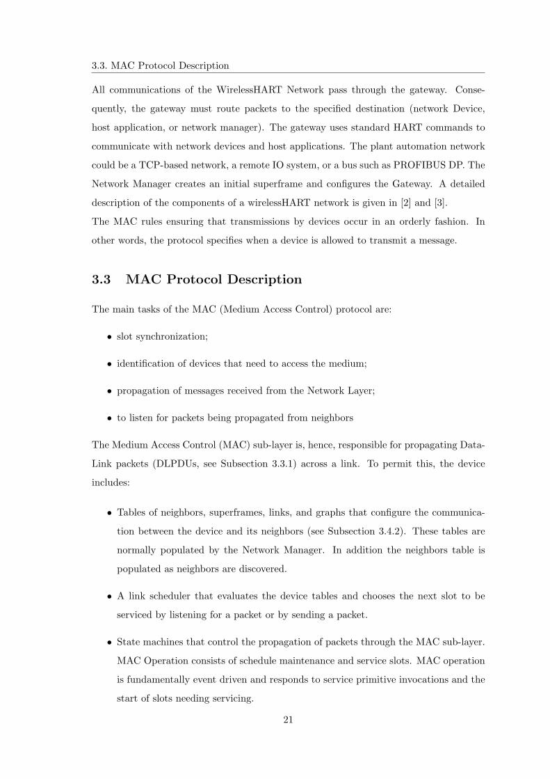
This subsection specifies the format of the Data-Link packet (DLPDU, see Figure 3.3).
Each DLPDU consists of the following fields:
• A single byte set to 0x41
• A 1-byte address specifier;
• The 1-byte Sequence Number;
• The 2 byte Network ID;
• Destination and Source Addresses either of which can be 2 or 8-bytes long;
• A 1-byte DLPDU Specifier;
• The DLL payload;
• A 4-byte keyed Message Integrity Code (MIC);
• A 2-byte ITU-T CRC16;
Figure 3.3: The DLPDU structure [1]
The total packet length is 127 bytes.
3.3.2 Time Division Multiple Access (TDMA)
WirelessHART uses Time Division Multiple Access (TDMA) and channel hopping to con-
trol access to the network. TDMA is a widely used Medium Access Control technique
22
3.3. MAC Protocol Description
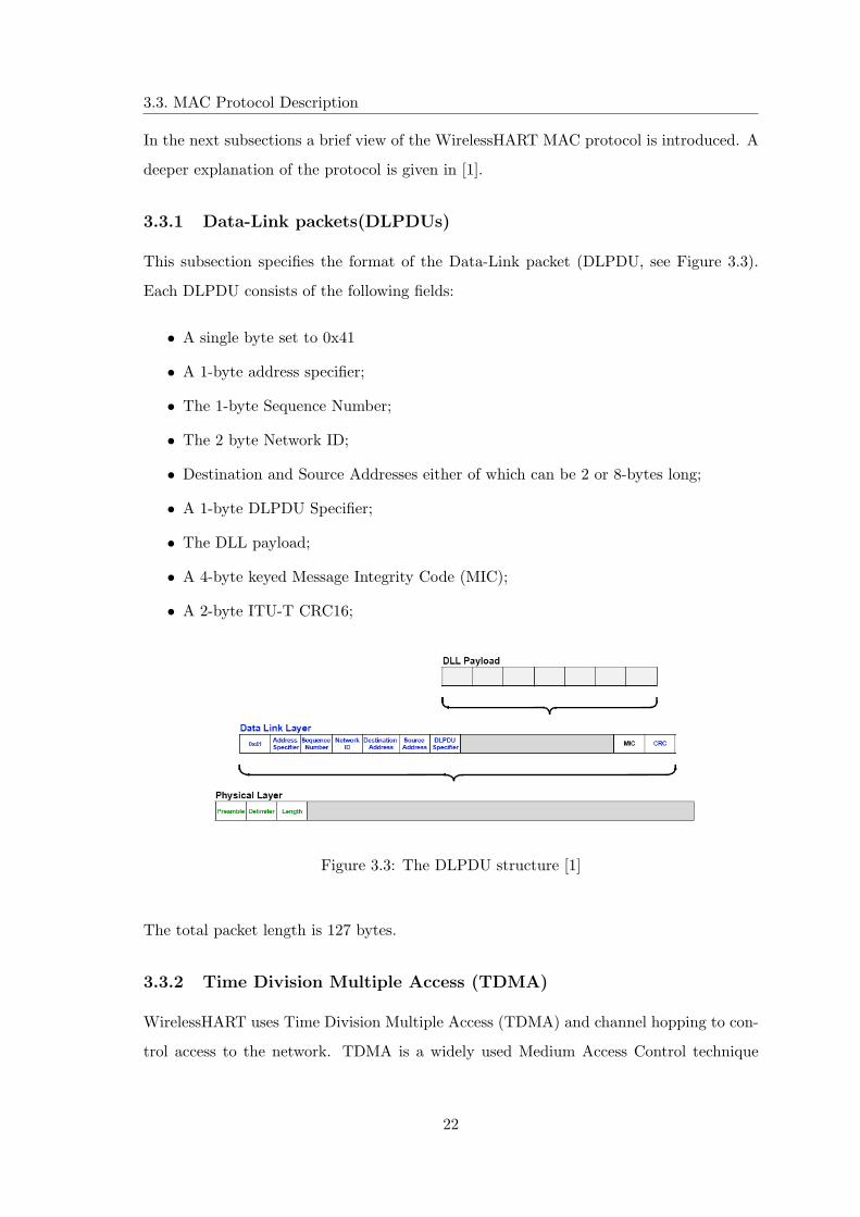
that provides collision free, deterministic communications. It uses time slots where com-
munications between devices occur. A series of time slots form a TDMA superframe (see
Figure 3.4).
Figure 3.4: The SuperFrame structure [1]
All devices must support multiple superframes. Slot sizes and the superframe length (in
number of slots) are fixed and form a network cycle with a fixed repetition rate. Super-
frames are repeated continuously. For successful and efficient TDMA communications,
synchronization of clocks between devices in the network is critical [26]. Consequently,
tolerances on time keeping and time synchronization mechanisms are specified to ensure
network-wide device clock synchronization. It is imperative that devices know when the
start of a slot occurs. Within the slot, transmission of the source message starts at a
specified time after the beginning of a slot. This short time delay allows the source and
destination to set their frequency channel and allows the receiver to begin listening on the
specified channel. Since there is a tolerance on clocks, the receiver must start to listen
before the ideal transmission start time and continue listening after that ideal time. Once
the transmission is complete, the communication direction is reversed and the destination
device indicates, by transmitting an ACK, whether it received the source device DLPDU
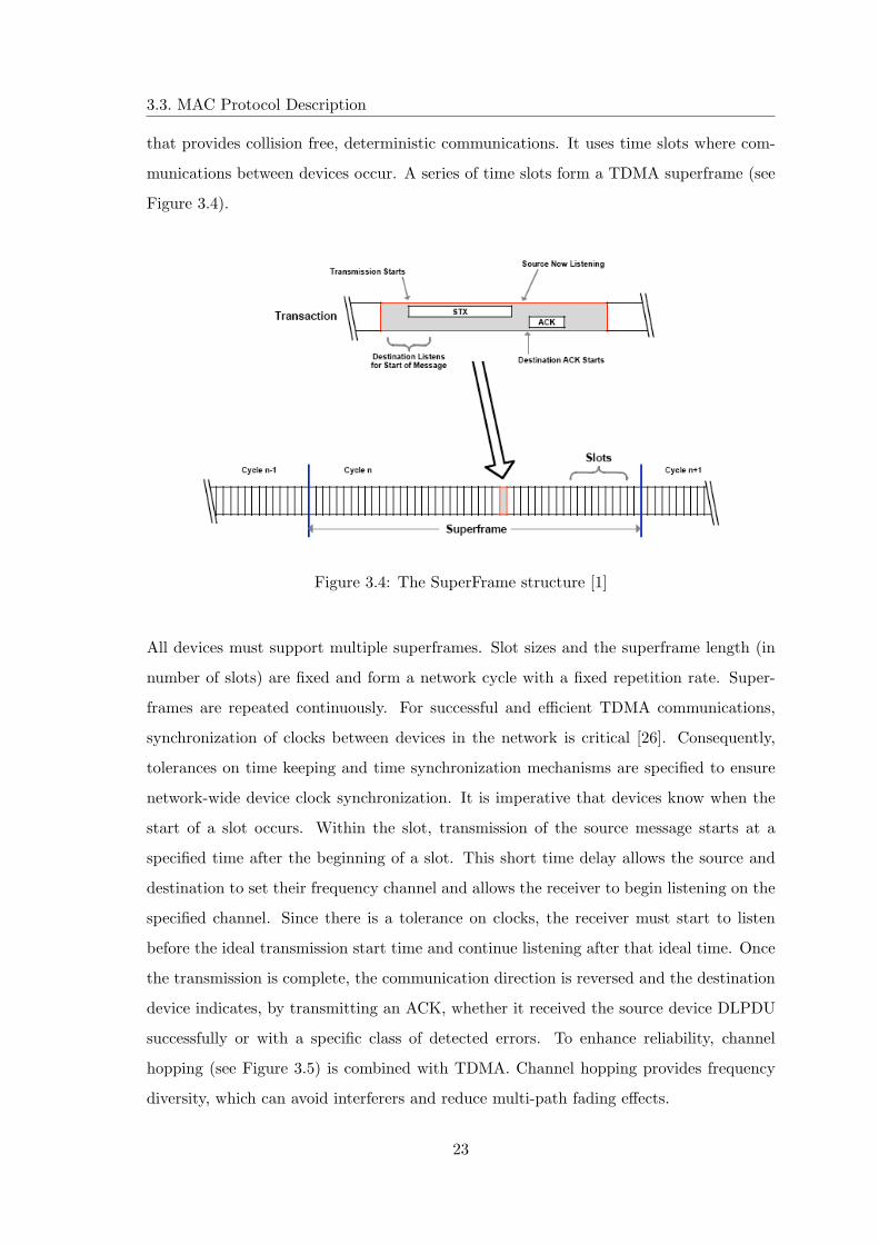
successfully or with a specific class of detected errors. To enhance reliability, channel
hopping (see Figure 3.5) is combined with TDMA. Channel hopping provides frequency
diversity, which can avoid interferers and reduce multi-path fading effects.
23
3.3. MAC Protocol Description
Figure 3.5: The channel hopping [1]
Communicating devices are assigned to a superframe, slot, and channel offset. This forms
a communications link between communicating devices.
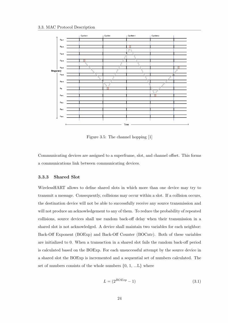
3.3.3 Shared Slot
WirelessHART allows to define shared slots in which more than one device may try to
transmit a message. Consequently, collisions may occur within a slot. If a collision occurs,
the destination device will not be able to successfully receive any source transmission and
will not produce an acknowledgement to any of them. To reduce the probability of repeated
collisions, source devices shall use random back-off delay when their transmission in a
shared slot is not acknowledged. A device shall maintain two variables for each neighbor:
Back-Off Exponent (BOExp) and Back-Off Counter (BOCntr). Both of these variables
are initialized to 0. When a transaction in a shared slot fails the random back-off period
is calculated based on the BOExp. For each unsuccessful attempt by the source device in
a shared slot the BOExp is incremented and a sequential set of numbers calculated. The
set of numbers consists of the whole numbers {0, 1, ...L} where
L = (2BOExp − 1) (3.1)
24
3.3. MAC Protocol Description
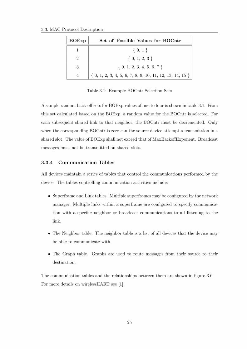
BOExp Set of Possible Values for BOCntr
1 { 0, 1 }2 { 0, 1, 2, 3 }3 { 0, 1, 2, 3, 4, 5, 6, 7 }4 { 0, 1, 2, 3, 4, 5, 6, 7, 8, 9, 10, 11, 12, 13, 14, 15 }
Table 3.1: Example BOCntr Selection Sets
A sample random back-off sets for BOExp values of one to four is shown in table 3.1. From
this set calculated based on the BOExp, a random value for the BOCntr is selected. For
each subsequent shared link to that neighbor, the BOCntr must be decremented. Only
when the corresponding BOCntr is zero can the source device attempt a transmission in a
shared slot. The value of BOExp shall not exceed that of MaxBackoffExponent. Broadcast
messages must not be transmitted on shared slots.
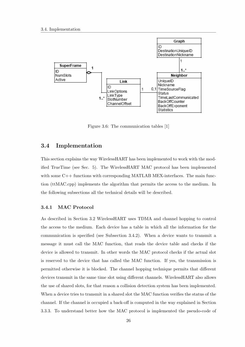
3.3.4 Communication Tables
All devices maintain a series of tables that control the communications performed by the
device. The tables controlling communication activities include:
• Superframe and Link tables. Multiple superframes may be configured by the network
manager. Multiple links within a superframe are configured to specify communica-
tion with a specific neighbor or broadcast communications to all listening to the
link.
• The Neighbor table. The neighbor table is a list of all devices that the device may
be able to communicate with.
• The Graph table. Graphs are used to route messages from their source to their
destination.
The communication tables and the relationships between them are shown in figure 3.6.
For more details on wirelessHART see [1].
25
3.4. Implementation
Figure 3.6: The communication tables [1]
3.4 Implementation
This section explains the way WirelessHART has been implemented to work with the mod-
ified TrueTime (see Sec. 5). The WirelessHART MAC protocol has been implemented
with some C++ functions with corresponding MATLAB MEX-interfaces. The main func-
tion (ttMAC.cpp) implements the algorithm that permits the access to the medium. In
the following subsections all the technical details will be described.
3.4.1 MAC Protocol
As described in Section 3.2 WirelessHART uses TDMA and channel hopping to control
the access to the medium. Each device has a table in which all the information for the
communication is specified (see Subsection 3.4.2). When a device wants to transmit a
message it must call the MAC function, that reads the device table and checks if the
device is allowed to transmit. In other words the MAC protocol checks if the actual slot
is reserved to the device that has called the MAC function. If yes, the transmission is
permitted otherwise it is blocked. The channel hopping technique permits that different
devices transmit in the same time slot using different channels. WirelessHART also allows
the use of shared slots, for that reason a collision detection system has been implemented.
When a device tries to transmit in a shared slot the MAC function verifies the status of the
channel. If the channel is occupied a back-off is computed in the way explained in Section
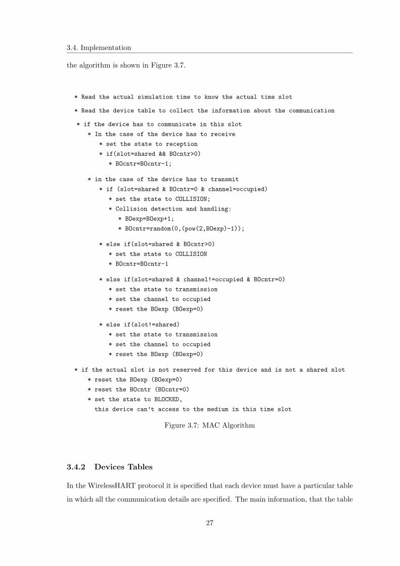
3.3.3. To understand better how the MAC protocol is implemented the pseudo-code of
26
3.4. Implementation
the algorithm is shown in Figure 3.7.
* Read the actual simulation time to know the actual time slot
* Read the device table to collect the information about the communication
* if the device has to communicate in this slot
* In the case of the device has to receive
* set the state to reception
* if(slot=shared && BOcntr>0)
* BOcntr=BOcntr-1;
* in the case of the device has to transmit
* if (slot=shared & BOcntr=0 & channel=occupied)
* set the state to COLLISION;
* Collision detection and handling:
* BOexp=BOexp+1;
* BOcntr=random(0,(pow(2,BOexp)-1));
* else if(slot=shared & BOcntr>0)
* set the state to COLLISION
* BOcntr=BOcntr-1
* else if(slot=shared & channel!=occupied & BOcntr=0)
* set the state to transmission
* set the channel to occupied
* reset the BOexp (BOexp=0)
* else if(slot!=shared)
* set the state to transmission
* set the channel to occupied
* reset the BOexp (BOexp=0)
* if the actual slot is not reserved for this device and is not a shared slot
* reset the BOexp (BOexp=0)
* reset the BOcntr (BOcntr=0)
* set the state to BLOCKED,
this device can’t access to the medium in this time slot
Figure 3.7: MAC Algorithm
3.4.2 Devices Tables
In the WirelessHART protocol it is specified that each device must have a particular table
in which all the communication details are specified. The main information, that the table
27
3.4. Implementation
must contain, are the time slots in which the device has to communicate, the information
for the channel hopping technique, the device with which the communication has to be
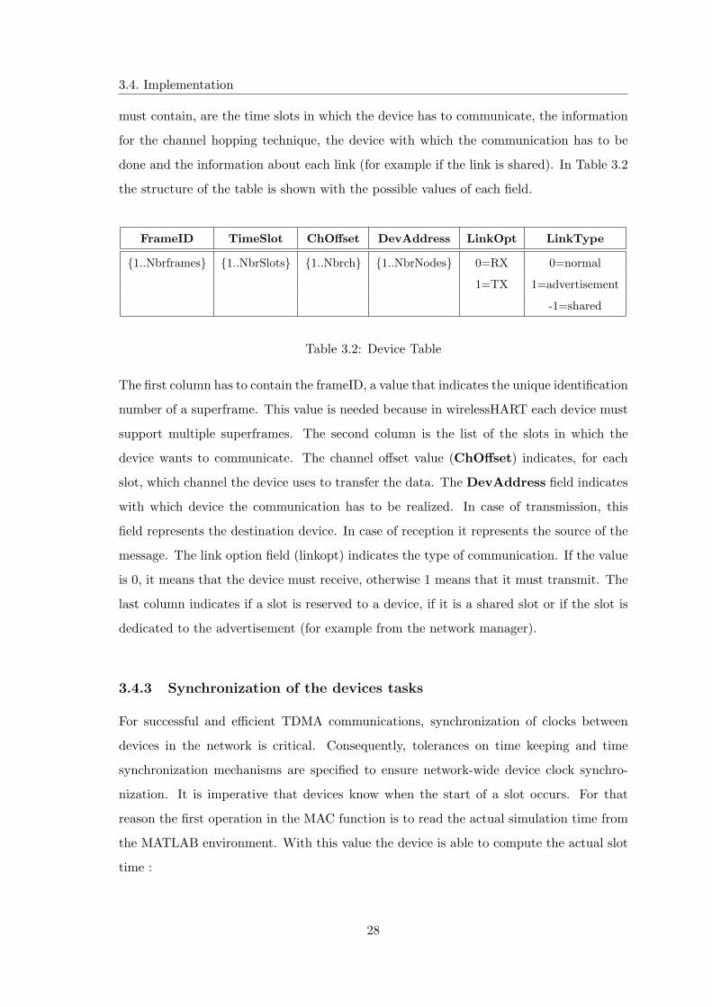
done and the information about each link (for example if the link is shared). In Table 3.2
the structure of the table is shown with the possible values of each field.
FrameID TimeSlot ChOffset DevAddress LinkOpt LinkType
{1..Nbrframes} {1..NbrSlots} {1..Nbrch} {1..NbrNodes} 0=RX 0=normal
1=TX 1=advertisement
-1=shared
Table 3.2: Device Table
The first column has to contain the frameID, a value that indicates the unique identification
number of a superframe. This value is needed because in wirelessHART each device must
support multiple superframes. The second column is the list of the slots in which the
device wants to communicate. The channel offset value (ChOffset) indicates, for each
slot, which channel the device uses to transfer the data. The DevAddress field indicates
with which device the communication has to be realized. In case of transmission, this
field represents the destination device. In case of reception it represents the source of the
message. The link option field (linkopt) indicates the type of communication. If the value
is 0, it means that the device must receive, otherwise 1 means that it must transmit. The
last column indicates if a slot is reserved to a device, if it is a shared slot or if the slot is
dedicated to the advertisement (for example from the network manager).
3.4.3 Synchronization of the devices tasks
For successful and efficient TDMA communications, synchronization of clocks between
devices in the network is critical. Consequently, tolerances on time keeping and time
synchronization mechanisms are specified to ensure network-wide device clock synchro-
nization. It is imperative that devices know when the start of a slot occurs. For that
reason the first operation in the MAC function is to read the actual simulation time from
the MATLAB environment. With this value the device is able to compute the actual slot
time :
28
3.4. Implementation
ActualSlotNumer = (Actual Sim time + exectime
SlotSize%SuperframeSize) + 1 (3.2)
where the exectime is the execution time of the device task that has called the MAC
function. The SlotSize is fixed to 10 ms in WirelessHART and the SuperframeSize is the
number of slots contained in a superframe (typically 100 slots, i.e. a superframe length of
1 s).
29
Chapter 4
Introduction to TrueTime
4.1 Description of the tool
This chapter describes the use of the original Matlab/Simulink-based simulator TrueTime
[5], which facilitates co-simulation of controller task execution in real-time kernels, network
transmissions (using wired or wireless networks), and continuous plant dynamics. In the
next chapter will be described the changes that have been made in this project. TrueTime
is not constituted by only the blocks library, but also by a collection of C++ functions
with corresponding MATLAB MEX-interfaces. Some functions permit to configure the
simulation by creating tasks, interrupt handlers, monitors, timers, etc. The other functions
are real-time primitives that are called from the task code during execution and provides
for AD-DA conversion, changing task attributes, entering and leaving monitors, sending
and receiving network messages, etc. TrueTime is developed in Simulink, which allows for
traditional control system assessment in terms of performance, stability and robustness.
TrueTime is primarily intended to be used together with MATLAB/Simulink. However,
the TrueTime kernel implements a complete event-based kernel and Simulink is only used
to interface the kernel and the tasks with the continuous-time processes.
30
4.1. Description of the tool
Being written in C++, it is easy to adapt the block code to other simulation environments.
All TrueTime objects, such as tasks, interrupt handlers, monitors, timers and events, are
defined by C++ classes that are easily extendable by the user to add more functionality.
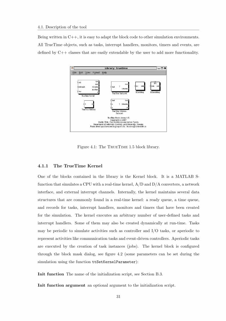
Figure 4.1: The TrueTime 1.5 block library.
4.1.1 The TrueTime Kernel
One of the blocks contained in the library is the Kernel block. It is a MATLAB S-
function that simulates a CPU with a real-time kernel, A/D and D/A converters, a network
interface, and external interrupt channels. Internally, the kernel maintains several data
structures that are commonly found in a real-time kernel: a ready queue, a time queue,
and records for tasks, interrupt handlers, monitors and timers that have been created
for the simulation. The kernel executes an arbitrary number of user-defined tasks and
interrupt handlers. Some of them may also be created dynamically at run-time. Tasks
may be periodic to simulate activities such as controller and I/O tasks, or aperiodic to
represent activities like communication tasks and event-driven controllers. Aperiodic tasks
are executed by the creation of task instances (jobs). The kernel block is configured
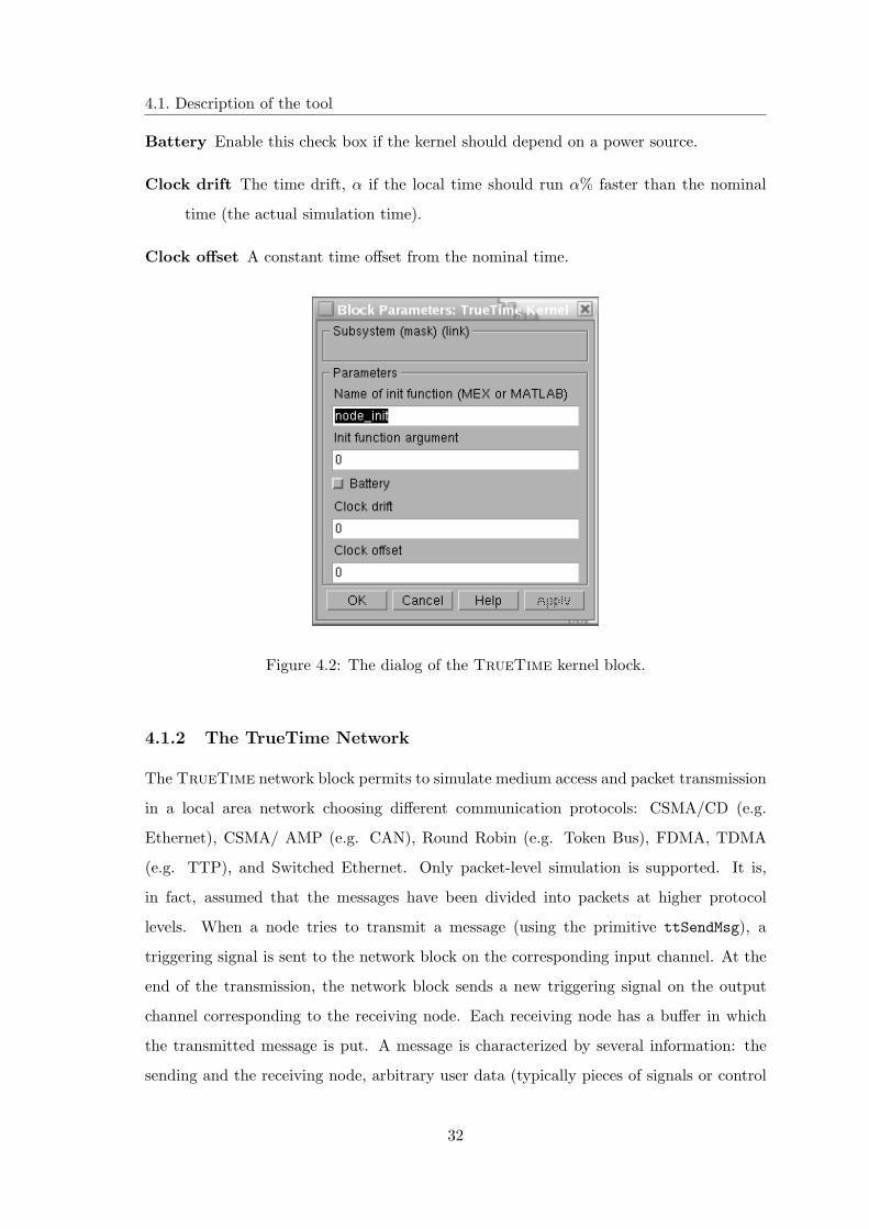
through the block mask dialog, see figure 4.2 (some parameters can be set during the
simulation using the function ttSetKernelParameter):
Init function The name of the initialization script, see Section B.3.
Init function argument an optional argument to the initialization script.
31
4.1. Description of the tool
Battery Enable this check box if the kernel should depend on a power source.
Clock drift The time drift, α if the local time should run α% faster than the nominal
time (the actual simulation time).
Clock offset A constant time offset from the nominal time.
Figure 4.2: The dialog of the TrueTime kernel block.
4.1.2 The TrueTime Network
The TrueTime network block permits to simulate medium access and packet transmission
in a local area network choosing different communication protocols: CSMA/CD (e.g.
Ethernet), CSMA/ AMP (e.g. CAN), Round Robin (e.g. Token Bus), FDMA, TDMA
(e.g. TTP), and Switched Ethernet. Only packet-level simulation is supported. It is,
in fact, assumed that the messages have been divided into packets at higher protocol
levels. When a node tries to transmit a message (using the primitive ttSendMsg), a
triggering signal is sent to the network block on the corresponding input channel. At the
end of the transmission, the network block sends a new triggering signal on the output
channel corresponding to the receiving node. Each receiving node has a buffer in which
the transmitted message is put. A message is characterized by several information: the
sending and the receiving node, arbitrary user data (typically pieces of signals or control
32
4.1. Description of the tool
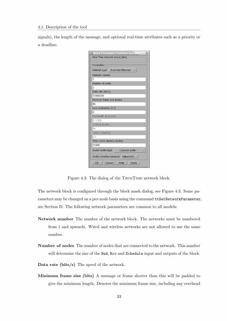
signals), the length of the message, and optional real-time attributes such as a priority or
a deadline.
Figure 4.3: The dialog of the TrueTime network block.
The network block is configured through the block mask dialog, see Figure 4.3. Some pa-
rameters may be changed on a per-node basis using the command ttSetNetworkParameter,
see Section D. The following network parameters are common to all models:
Network number The number of the network block. The networks must be numbered
from 1 and upwards. Wired and wireless networks are not allowed to use the same
number.
Number of nodes The number of nodes that are connected to the network. This number
will determine the size of the Snd, Rcv and Schedule input and outputs of the block.
Data rate (bits/s) The speed of the network.
Minimum frame size (bits) A message or frame shorter than this will be padded to
give the minimum length. Denotes the minimum frame size, including any overhead
33
4.1. Description of the tool
introduced by the protocol. E.g., the minimum Ethernet frame size, including a
14-byte header and a 4-byte CRC, is 512 bits.
Pre-processing delay (s) The time a message is delayed by the network interface on
the sending end. This can be used to model, e.g., a slow serial connection between
the computer and the network interface.
Post-processing delay (s) The time a message is delayed by the network interface on
the receiving end.
Loss probability (0–1) The probability that a network message is lost during transmis-
sion. Lost messages will consume network bandwidth, but will never arrive at the
destination.
4.1.3 The TrueTime Wireless Network
The Wireless Network block (see Section 4.2 for more details) permits to simulate, like
the one described in the last section, the communication between two nodes. It takes
into account also the path-loss of the radio signals. The possibility to lose packets is
modelled considering the spacial location of the nodes, the power transmission used and
some other statistical parameters. Only two network protocols were supported originally:
IEEE 802.11b/g (WLAN) and IEEE 802.15.4 (ZigBee). WirelessHART has been added
(see Sec. 3.4.1 and 5.7). The radio model used includes support for:
• Ad-hoc wireless networks.
• Isotropic antenna.
• Inability to send and receive messages at the same time.
• Path loss of radio signals modeled as 1da where d is the distance in meters and a is
a parameter chosen to model the environment.
• Interference from other terminals.
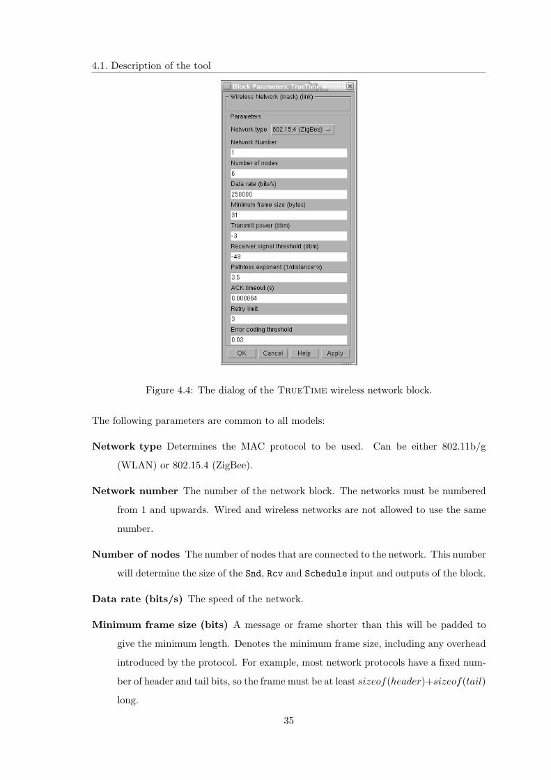
The wireless network block is configured through the block mask dialog, see Figure 4.4.
Using the command ttSetNetworkParameter some parameters can also be set on a per-
node basis.
34
4.1. Description of the tool
Figure 4.4: The dialog of the TrueTime wireless network block.
The following parameters are common to all models:
Network type Determines the MAC protocol to be used. Can be either 802.11b/g
(WLAN) or 802.15.4 (ZigBee).
Network number The number of the network block. The networks must be numbered
from 1 and upwards. Wired and wireless networks are not allowed to use the same
number.
Number of nodes The number of nodes that are connected to the network. This number
will determine the size of the Snd, Rcv and Schedule input and outputs of the block.
Data rate (bits/s) The speed of the network.
Minimum frame size (bits) A message or frame shorter than this will be padded to
give the minimum length. Denotes the minimum frame size, including any overhead
introduced by the protocol. For example, most network protocols have a fixed num-
ber of header and tail bits, so the frame must be at least sizeof(header)+sizeof(tail)
long.
35
4.1. Description of the tool
Transmit power Determines how strong the radio signal will be, and thereby how long
it will reach.
Receiver signal threshold If the received energy is above this threshold, then the
medium is accounted as busy.
Path-loss exponent The path loss of the radio signal is modeled as 1da where d is the
distance in meters and a is a suitably chosen parameter to model the environment.
Typically chosen in the interval 2-4.
ACK timeout The time a sending node will wait for an ACK message before concluding
that the message was lost and retransmit it.
Retry limit The maximum number of times a node will try to retransmit a message
before giving up.
Error coding threshold A number in the interval [0, 1] which defines the percentage of
block errors in a message that the coding can handle. For example, certain coding
schemes can fully reconstruct a message if it has less than 3% block errors. The
number of block errors are calculated using the signal-to-noise ratio, where the noise
is all other ongoing transmissions.
4.1.4 The TrueTime Standalone Network Blocks
The standalone network blocks are two, the ttSendMsg and the ttGetMsg. They can
be used to send messages using the network blocks without using kernel blocks (see Sec.
4.1.1). This permits (not having to initialize kernels, create and install interrupt handlers,
etc.) to build quickly a simulation, without create any M-files.
The standalone network blocks are configured through the block mask dialogs, seen in
Figure 4.5. The parameters are the same that are used in the ttSendMsg and ttGetMsg
primitives. The ttSendMsg block has a Simulink trigger input port, which can be config-
ured to trigger on raising, falling or either flanks. The ttGetMsg block has an optional
trigger output port whose value switches back and forth between 0 and 1 as messages
are received. It is useful to trigger any other block that has to be executed after a new
message has been received.
36
4.2. Wireless Network Block behaviour
Figure 4.5: The dialog of the ttGetMsg block to the left, and the dialog of the ttSendMsg
block to the right.
4.1.5 The TrueTime Battery
The battery block permits to set the initial power of a node using the configuration mask.
To use the battery, enable the check box in the kernel configuration mask and connect the
output of the battery to the E input of the kernel block. Connect every power drain such
as the P output of the kernel block, ordinary Simulink models, and the wireless network
block to the P input of the battery. The battery uses a simple integrator model, so it can
be both charged and recharged. If the kernel is configured to use batteries and the input
P to the kernel block is zero, it will not execute any code.
4.2 Wireless Network Block behaviour
The wireless network block simulates medium access and packet transmission. Originally
it implemented two kinds of communication protocols, 802.11b/g (WLAN) and 802.15.4
(ZigBee). The possibility to use also WirelessHART has been added. The block permits
37
4.2. Wireless Network Block behaviour
to simulate packets lost using a packet error probability or specifying when a packet has to
be discharged. It permits to compare more simulations together taking into account how
the same sequence of packets lost affects them. In the following subsection the original
options of the network will be carefully described. The new possibilities added in this
project, instead, are described in chapter 5
4.2.1 802.11b/g (WLAN)
IEEE 802.11b/g are two of the more popular protocols used today. IEEE 802.11 is used
in many laptops and mobile devices. The protocol is based on CSMA/CA with some
modifications. In TrueTime a package transmission is modelled like this: The node that
wants to transmit a packet checks if the medium is idle. The transmission may proceed,
if the medium is found to be idle, and has stayed so for 50 µs. If, on the other hand,
the medium is found to be busy, a random back-off time is chosen and decremented in
the same way as when colliding (described later in this section). When a node starts to
transmit, its relative position to all other nodes in the same network is calculated, and the
signal level in all those nodes are calculated according to the path-loss formula 1/da. If the
signal level in the receiving node is larger than the receiver signal threshold, then the
signal-to-noise ratio (SNR) is calculated and used to find the block error rate (BLER). All
other transmissions add to the background noise when calculating the SNR. The BLER
and the size of the message are used together to calculate the number of bit errors in the
message. If the percentage of bit errors is lower than the error coding threshold, then
it is assumed that the channel coding scheme is able to fully reconstruct the message.
If any other nodes are already transmitting to the receiving node and their respective
SNRs are lower than the new one or if there are other ongoing transmissions which the
currently sending node reaches with its transmission, then all those messages are marked
as collided and discharged. From the perspective of the sending node, lost messages and
message collisions are the same. ACK messages are sent on the MAC protocol layer. If
the ACK is not received by the transmitting node during ACK timeout, the message
is retransmitted after waiting a random back-off time within a contention window. The
contention window size is doubled for every retransmission of a certain message. The
back-off timer is decremented only if the medium is idle, or if it has been idle for at least
50 µs. The Retry limit number of retransmissions specifies the maximum number of
38
4.2. Wireless Network Block behaviour
times that a message could be retransmitted before it is discharged.
4.2.2 802.15.4 (ZigBee)
ZigBee is a protocol optimized for the use of sensors and simple control networks. It is
characterized by a rather low bandwidth and by a really low power consumption that
increases the life of the devices from a battery consumption point of view. It is based on
CSMA/CA.
The packet transmission model in ZigBee is similar to WLAN, but the MAC procedure
differs and is modeled as:
1. Initialize:
NB=0
BE=macMinBE
2. Delay for a random number of backoff periods (order of 100 µs) in the interval
[0, 2BE − 1]
3. Is the medium idle?
if yes: send
else: goto 4
4. Update the backoff counters:
NB=NB+1
BE=min(BE+1, aMaxBE)
5. Is NB>macMaxCSMABackoffs?
if yes: drop the packet
else: goto 2
where:
NB Number of backoffs.
BE Backoff exponent.
macMinBE The minimum value of the backoff exponent in the CSMA/CA algorithm.
The default value is 3.
39
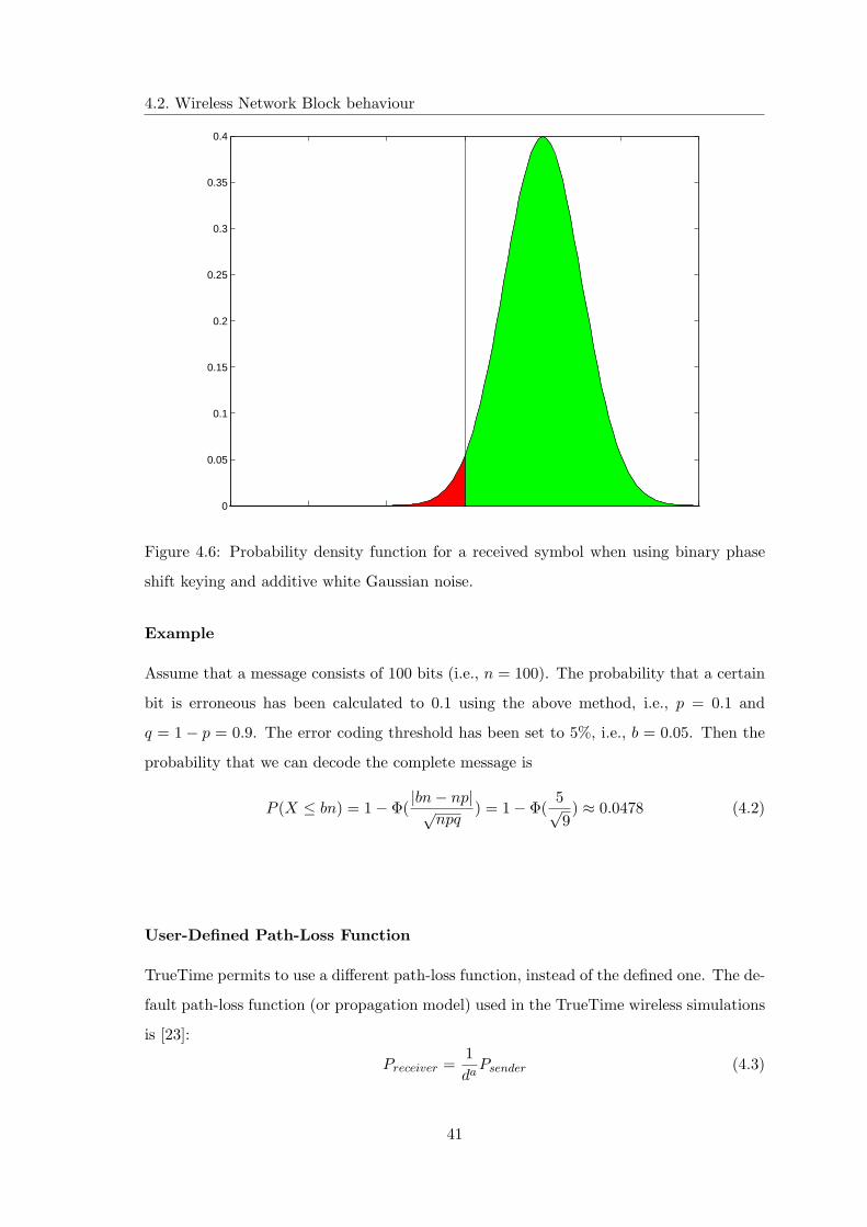
4.2. Wireless Network Block behaviour
aMaxBE The maximum value of the backoff exponent in the CSMA/CA algorithm. The
default value is 5.
macMaxCSMABackoffs The maximum number of backoffs the CSMA/CA algorithm
will attempt before declaring a channel access failure. The default value is 4.
The variable names are taken from the standard to make comparisons easier.
4.2.3 Calculation of Error Probabilities
When a symbol is sent, in this case it is a bit, an additive white Gaussian noise gives a
probability density function for the received symbol, that for some signal-to-noise ratio
may look like Figure 4.6. A threshold is then used to decide if the received symbol is a 0
or a 1. The darker area to the left of the threshold gives the probability of a symbol error.
A higher signal to noise ratio translates the curve to the right, making the probability of
error smaller. During the calculation of error probabilities, the following approximation is
done: BPSK1 is always used in the transmissions.
The above standard procedure takes into account the single bits that form a message.
The total number of calculated bit errors should then be compared to the error coding
threshold. Being it very computationally expensive, it has been chosen to save the max-
imum noise level during the transmission and to use it to calculate the worst case SNR.
By assuming that bit errors in a message are uncorrelated, it is deduced that the number
of bit errors, X, belongs to a binomial distribution X ∈ Bin(n, p), where n is the number
of bits in the message, and p is the probability that a certain bit is erroneous. If the value
of n is large, the binomial distribution can be approximated with a normal distribution,
using the central limit theorem. This gives that X ∈ N(np,√
npq) where q = 1−p. What
we are really interested in is the probability that bn, where b is the error coding threshold,
is larger than the total number of bit errors in a message.
This probability is calculated using
P (X ≤ bn) =
Φ(bn− np√
npq) if bn− np > 0
1− Φ(|bn− np|√
npq) if bn− np ≤ 0
(4.1)
where Φ is the standard normal cumulative distribution function.1Binary Phase Shift Keying (BPSK) is a means of transmitting symbols by altering the phase of a
reference signal. It uses two phases separated by 180◦ and is hence binary.
40
4.2. Wireless Network Block behaviour
0
0.05
0.1
0.15
0.2
0.25
0.3
0.35
0.4
Figure 4.6: Probability density function for a received symbol when using binary phase
shift keying and additive white Gaussian noise.
Example
Assume that a message consists of 100 bits (i.e., n = 100). The probability that a certain
bit is erroneous has been calculated to 0.1 using the above method, i.e., p = 0.1 and
q = 1− p = 0.9. The error coding threshold has been set to 5%, i.e., b = 0.05. Then the
probability that we can decode the complete message is
P (X ≤ bn) = 1− Φ(|bn− np|√
npq) = 1− Φ(
5√9) ≈ 0.0478 (4.2)
User-Defined Path-Loss Function
TrueTime permits to use a different path-loss function, instead of the defined one. The de-
fault path-loss function (or propagation model) used in the TrueTime wireless simulations
is [23]:
Preceiver =1da
Psender (4.3)
41
4.2. Wireless Network Block behaviour
where P is the power, d is the distance in meters, and a is a parameter that can be chosen
to model different environments. This model is often used in simulations, but if the user
prefers to implement his own function, he may do it by writing a Matlab m-file where all
the built-in functions available in Matlab or Simulink could be called.
The Matlab function has to take the following arguments
• Transmission power
• Name of the sending node
• x and y coordinates of the sending node
• Name of the receiving node
• x and y coordinates of the receiving node
• Current simulation time
and return the signal power in the receiving node.
42
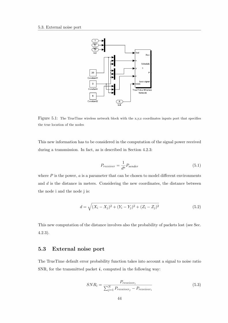
Chapter 5
New functions in the wireless
network block
5.1 Introduction
In this chapter will be described some new utilities implemented to improve the behavior
and the useability of the wireless network block of TrueTime. In Section 5.2 the 3D
location of the nodes is described. It permits a more realistic placement of the devices in
the environment. Another useful functionality is introduced in Section 5.3 and it consists
in the possibility to introduce an external source of noise. Section 5.4 explains a new way
for the computation of the noise considering a time correlation between the time samples.
To improve the usability of the tool the possibility to notice when a packet is lost has
been added (Section 5.5). Section 5.6 explains a new option that permits to simulate, in a
deterministic way, a time interval in which the network loses packets. Section 5.7 describes
the modification in the TrueTime graphic interface, of the wireless network block, done
to use the WirelessHART protocol. For a more realistic behavior of the devices the MAC
layer has been moved from the wireless network block and implemented in a separate
function that can be called from each device (Section 5.8).
5.2 Nodes in the 3D space
TrueTime allows to collocate the devices on a 2D plane. It does not permit to build up a
real scenario in which the nodes could be placed at different heights, for example attached
to the same column. For that reason, the possibility to specify the (X,Y,Z) coordinates
(meters) in the space for each node is given (see Fig. 5.1).
43
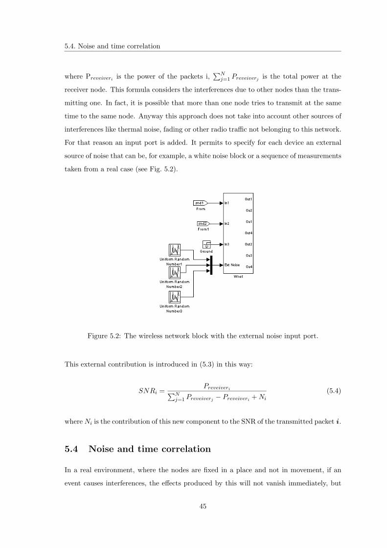
5.3. External noise port
Figure 5.1: The TrueTime wireless network block with the x,y,z coordinates inputs port that specifies
the true location of the nodes
This new information has to be considered in the computation of the signal power received
during a transmission. In fact, as is described in Section 4.2.3:
Preceiver =1da
Psender (5.1)
where P is the power, a is a parameter that can be chosen to model different environments
and d is the distance in meters. Considering the new coordinates, the distance between
the node i and the node j is:
d =√
(Xi −Xj)2 + (Yi − Yj)2 + (Zi − Zj)2 (5.2)
This new computation of the distance involves also the probability of packets lost (see Sec.
4.2.3).
5.3 External noise port
The TrueTime default error probability function takes into account a signal to noise ratio
SNR, for the transmitted packet i , computed in the following way:
SNRi =Preveiveri∑N
j=1 Preveiverj − Preveiveri
(5.3)
44
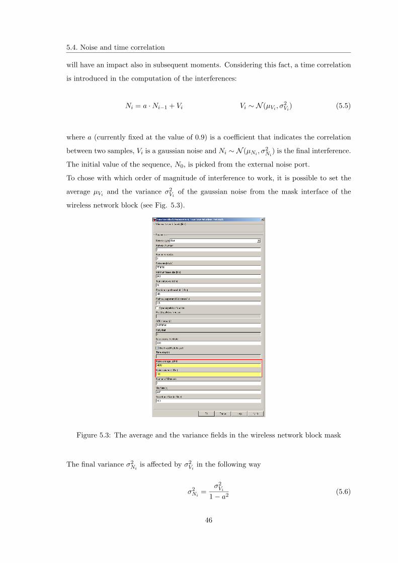
5.4. Noise and time correlation
where Preveiveri is the power of the packets i,∑N
j=1 Preveiverj is the total power at the
receiver node. This formula considers the interferences due to other nodes than the trans-
mitting one. In fact, it is possible that more than one node tries to transmit at the same
time to the same node. Anyway this approach does not take into account other sources of
interferences like thermal noise, fading or other radio traffic not belonging to this network.
For that reason an input port is added. It permits to specify for each device an external
source of noise that can be, for example, a white noise block or a sequence of measurements
taken from a real case (see Fig. 5.2).
Figure 5.2: The wireless network block with the external noise input port.
This external contribution is introduced in (5.3) in this way:
SNRi =Preveiveri∑N
j=1 Preveiverj − Preveiveri + Ni
(5.4)
where Ni is the contribution of this new component to the SNR of the transmitted packet i .
5.4 Noise and time correlation
In a real environment, where the nodes are fixed in a place and not in movement, if an
event causes interferences, the effects produced by this will not vanish immediately, but
45
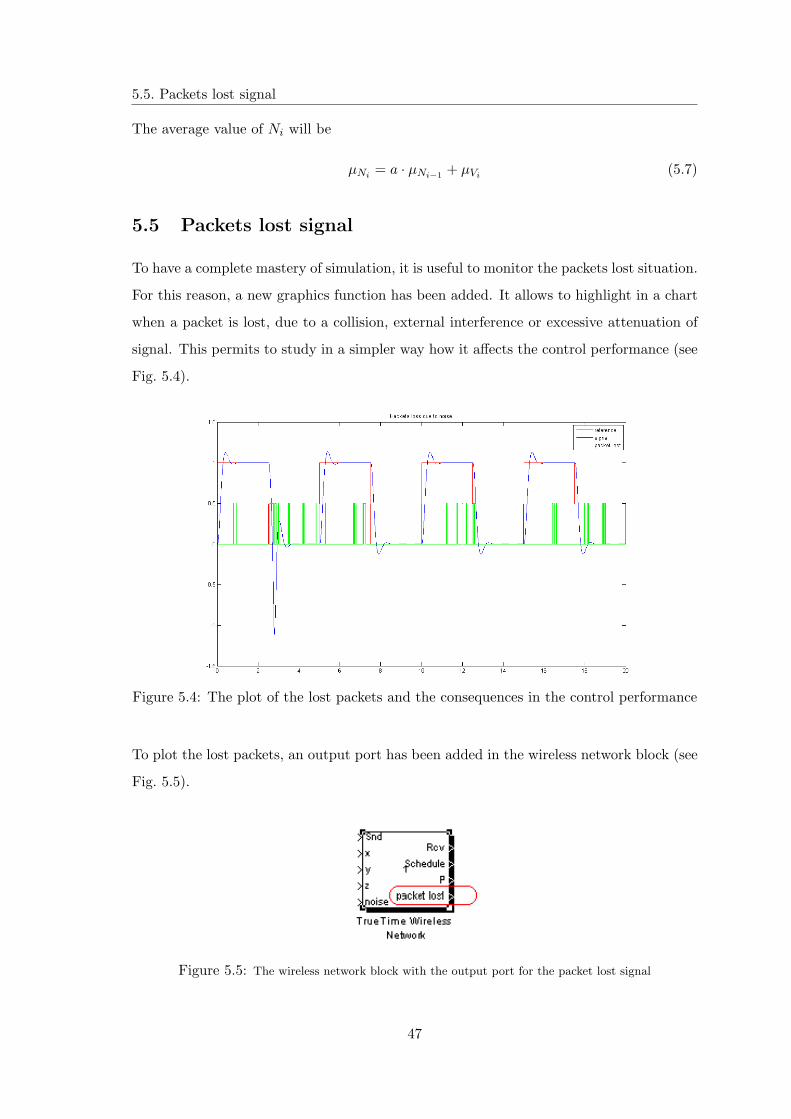
5.4. Noise and time correlation
will have an impact also in subsequent moments. Considering this fact, a time correlation
is introduced in the computation of the interferences:
Ni = a ·Ni−1 + Vi Vi ∼ N (µVi , σ2Vi
) (5.5)
where a (currently fixed at the value of 0.9) is a coefficient that indicates the correlation
between two samples, Vi is a gaussian noise and Ni ∼ N (µNi , σ2Ni
) is the final interference.
The initial value of the sequence, N0, is picked from the external noise port.
To chose with which order of magnitude of interference to work, it is possible to set the
average µVi and the variance σ2Vi
of the gaussian noise from the mask interface of the
wireless network block (see Fig. 5.3).
Figure 5.3: The average and the variance fields in the wireless network block mask
The final variance σ2Ni
is affected by σ2Vi
in the following way
σ2Ni
=σ2
Vi
1− a2(5.6)
46
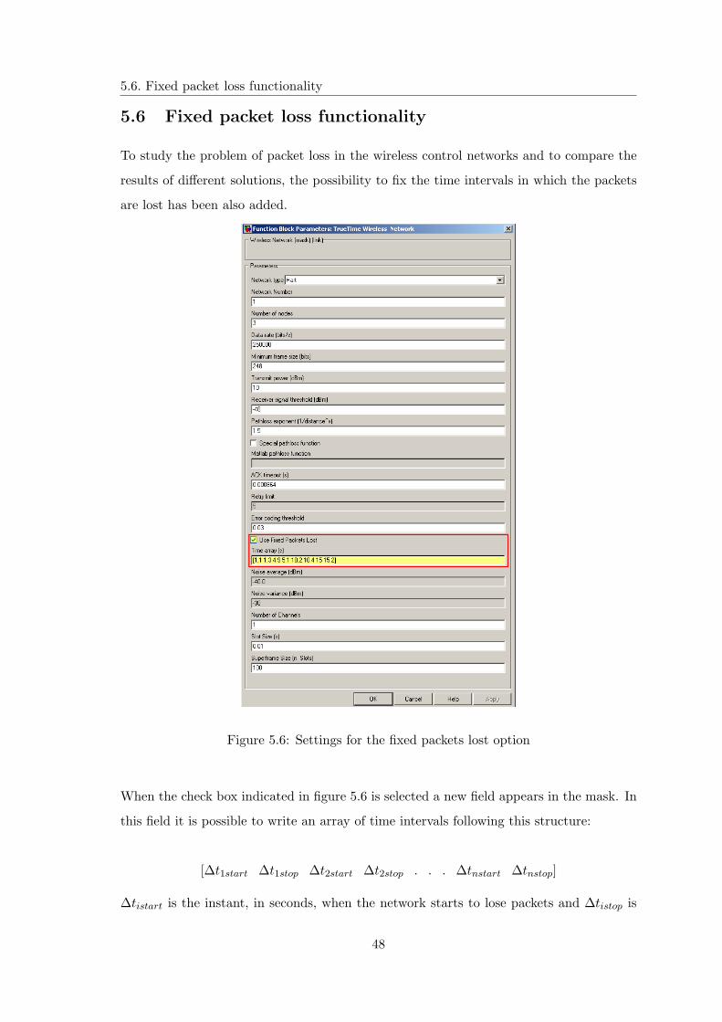
5.5. Packets lost signal
The average value of Ni will be
µNi = a · µNi−1 + µVi (5.7)
5.5 Packets lost signal
To have a complete mastery of simulation, it is useful to monitor the packets lost situation.
For this reason, a new graphics function has been added. It allows to highlight in a chart
when a packet is lost, due to a collision, external interference or excessive attenuation of
signal. This permits to study in a simpler way how it affects the control performance (see
Fig. 5.4).
Figure 5.4: The plot of the lost packets and the consequences in the control performance
To plot the lost packets, an output port has been added in the wireless network block (see
Fig. 5.5).
Figure 5.5: The wireless network block with the output port for the packet lost signal
47
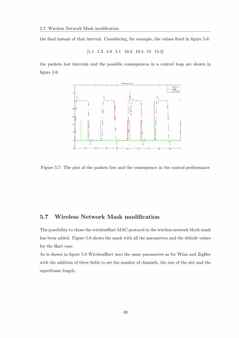
5.6. Fixed packet loss functionality
5.6 Fixed packet loss functionality
To study the problem of packet loss in the wireless control networks and to compare the
results of different solutions, the possibility to fix the time intervals in which the packets
are lost has been also added.
Figure 5.6: Settings for the fixed packets lost option
When the check box indicated in figure 5.6 is selected a new field appears in the mask. In
this field it is possible to write an array of time intervals following this structure:
[∆t1start ∆t1stop ∆t2start ∆t2stop . . . ∆tnstart ∆tnstop]
∆tistart is the instant, in seconds, when the network starts to lose packets and ∆tistop is
48
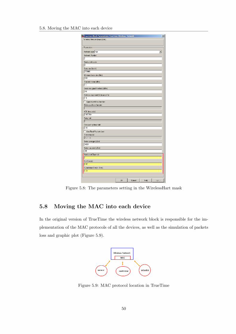
5.7. Wireless Network Mask modification
the final instant of that interval. Considering, for example, the values fixed in figure 5.6:
[1.1 1.3 4.9 5.1 10.2 10.4 15 15.2]
the packets lost intervals and the possible consequences in a control loop are shown in
figure 5.6.
Figure 5.7: The plot of the packets lost and the consequence in the control performance
5.7 Wireless Network Mask modification
The possibility to chose the wirelessHart MAC protocol in the wireless network block mask
has been added. Figure 5.8 shows the mask with all the parameters and the default values
for the Hart case.
As is shown in figure 5.8 WirelessHart uses the same parameters as for Wlan and ZigBee
with the addition of three fields to set the number of channels, the size of the slot and the
superframe length.
49
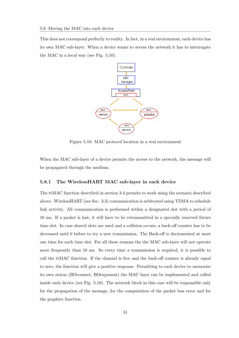
5.8. Moving the MAC into each device
Figure 5.8: The parameters setting in the WirelessHart mask
5.8 Moving the MAC into each device
In the original version of TrueTime the wireless network block is responsible for the im-
plementation of the MAC protocols of all the devices, as well as the simulation of packets
loss and graphic plot (Figure 5.9).
Figure 5.9: MAC protocol location in TrueTime
50
5.8. Moving the MAC into each device
This does not correspond perfectly to reality. In fact, in a real environment, each device has
its own MAC sub-layer. When a device wants to access the network it has to interrogate
the MAC in a local way (see Fig. 5.10).
Figure 5.10: MAC protocol location in a real environment
When the MAC sub-layer of a device permits the access to the network, the message will
be propagated through the medium.
5.8.1 The WirelessHART MAC sub-layer in each device
The ttMAC function described in section 3.4 permits to work using the scenario described
above. WirelessHART (see Sec. 3.3) communication is arbitrated using TDMA to schedule
link activity. All communication is performed within a designated slot with a period of
10 ms. If a packet is lost, it will have to be retransmitted in a specially reserved future
time slot. In case shared slots are used and a collision occurs, a back-off counter has to be
decreased until 0 before to try a new transmission. The Back-off is decremented at most
one time for each time slot. For all these reasons the the MAC sub-layer will not operate
more frequently than 10 ms. So every time a transmission is required, it is possible to
call the ttMAC function. If the channel is free and the back-off counter is already equal
to zero, the function will give a positive response. Permitting to each device to memorize
its own status (BOcounter, BOexponent) the MAC layer can be implemented and called
inside each device (see Fig. 5.10). The network block in this case will be responsible only
for the propagation of the message, for the computation of the packet loss error and for
the graphics function.
51
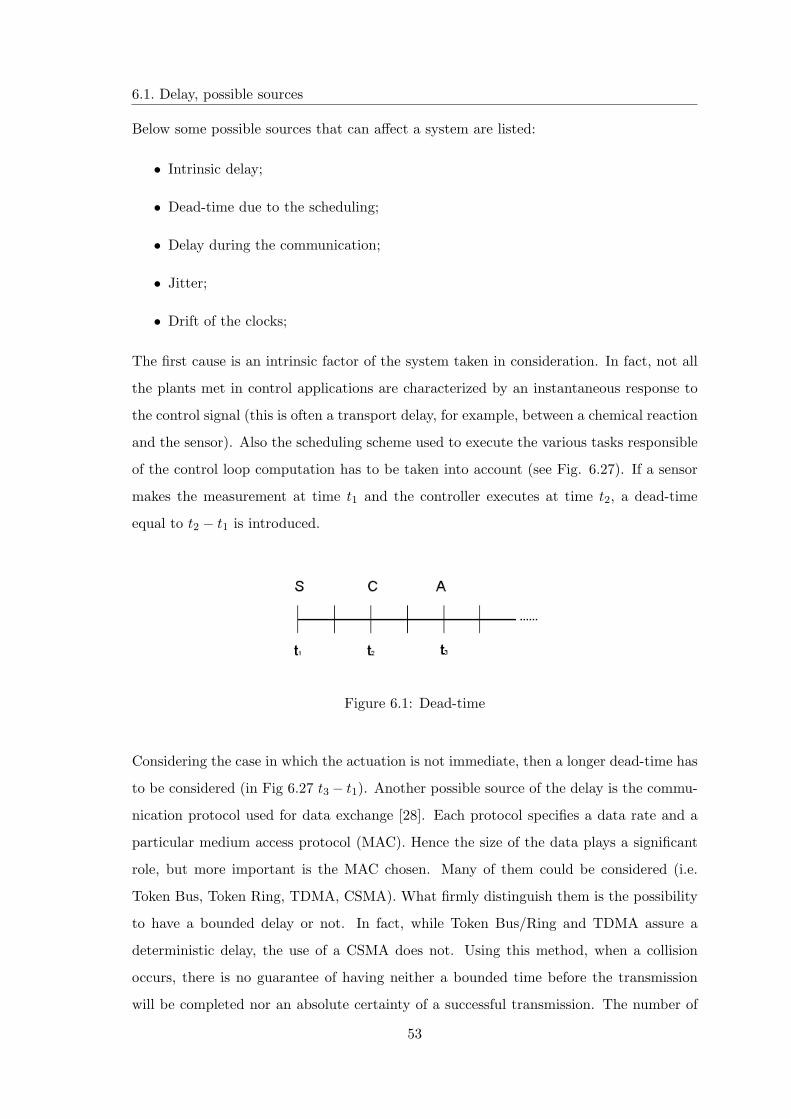
Chapter 6
Delay compensation
In this chapter will be described how the most common industrial model can be affected by
delay and some possible solutions to overcome this problem. In section 6.1 is introduced the
problem of the delay in a control loop and the possible sources. In 6.2 is investigated how
the performance of a control loop could be influenced by a delay considering some typical
industrial systems. Section 6.3 investigates some possible solutions that the controller can
adopt to improve its performance. A brief description of the controller AC800M is given
in 6.5. In Section 6.6 the problem of delay due to the clock drift in controllers like the
AC800M will be treated.
6.1 Delay, possible sources
The effects of delays in control loops can be really annoying and, in extreme case, bring
the system to instability. For these reasons it is of great importance to study the type of
delays presents in the plant that has to be controlled. The possible causes of delay in a
control system can be many.
52
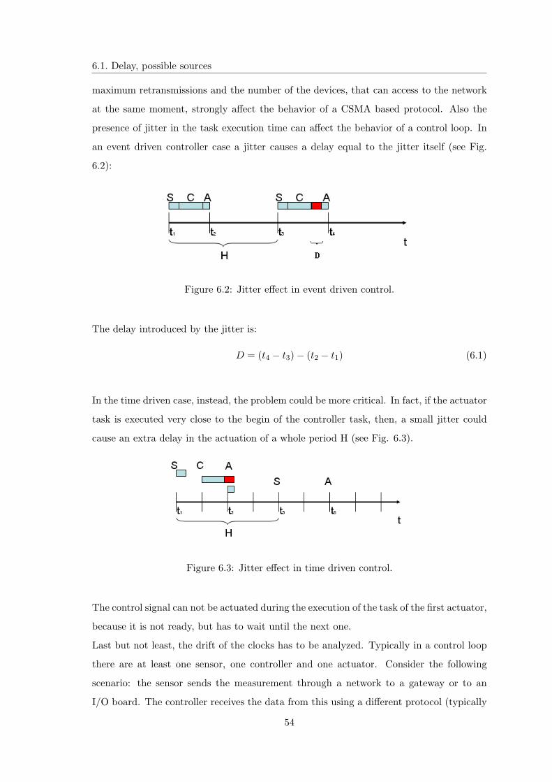
6.1. Delay, possible sources
Below some possible sources that can affect a system are listed:
• Intrinsic delay;
• Dead-time due to the scheduling;
• Delay during the communication;
• Jitter;
• Drift of the clocks;
The first cause is an intrinsic factor of the system taken in consideration. In fact, not all
the plants met in control applications are characterized by an instantaneous response to
the control signal (this is often a transport delay, for example, between a chemical reaction
and the sensor). Also the scheduling scheme used to execute the various tasks responsible
of the control loop computation has to be taken into account (see Fig. 6.27). If a sensor
makes the measurement at time t1 and the controller executes at time t2, a dead-time
equal to t2 − t1 is introduced.
Figure 6.1: Dead-time
Considering the case in which the actuation is not immediate, then a longer dead-time has
to be considered (in Fig 6.27 t3 − t1). Another possible source of the delay is the commu-
nication protocol used for data exchange [28]. Each protocol specifies a data rate and a
particular medium access protocol (MAC). Hence the size of the data plays a significant
role, but more important is the MAC chosen. Many of them could be considered (i.e.
Token Bus, Token Ring, TDMA, CSMA). What firmly distinguish them is the possibility
to have a bounded delay or not. In fact, while Token Bus/Ring and TDMA assure a
deterministic delay, the use of a CSMA does not. Using this method, when a collision
occurs, there is no guarantee of having neither a bounded time before the transmission
will be completed nor an absolute certainty of a successful transmission. The number of
53
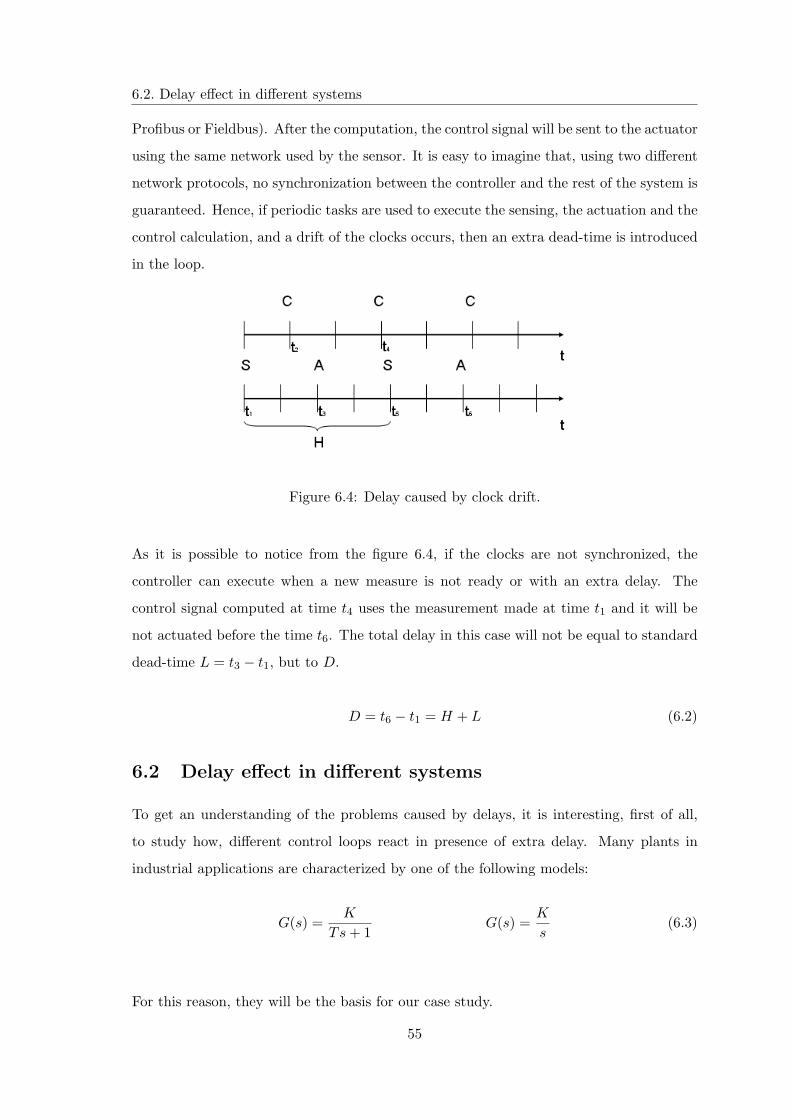
6.1. Delay, possible sources
maximum retransmissions and the number of the devices, that can access to the network
at the same moment, strongly affect the behavior of a CSMA based protocol. Also the
presence of jitter in the task execution time can affect the behavior of a control loop. In
an event driven controller case a jitter causes a delay equal to the jitter itself (see Fig.
6.2):
Figure 6.2: Jitter effect in event driven control.
The delay introduced by the jitter is:
D = (t4 − t3)− (t2 − t1) (6.1)
In the time driven case, instead, the problem could be more critical. In fact, if the actuator
task is executed very close to the begin of the controller task, then, a small jitter could
cause an extra delay in the actuation of a whole period H (see Fig. 6.3).
Figure 6.3: Jitter effect in time driven control.
The control signal can not be actuated during the execution of the task of the first actuator,
because it is not ready, but has to wait until the next one.
Last but not least, the drift of the clocks has to be analyzed. Typically in a control loop
there are at least one sensor, one controller and one actuator. Consider the following
scenario: the sensor sends the measurement through a network to a gateway or to an
I/O board. The controller receives the data from this using a different protocol (typically
54
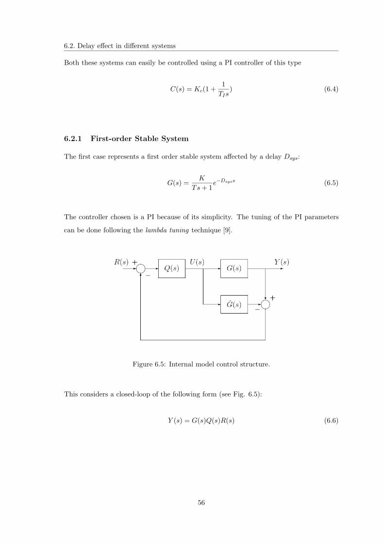
6.2. Delay effect in different systems
Profibus or Fieldbus). After the computation, the control signal will be sent to the actuator
using the same network used by the sensor. It is easy to imagine that, using two different
network protocols, no synchronization between the controller and the rest of the system is
guaranteed. Hence, if periodic tasks are used to execute the sensing, the actuation and the
control calculation, and a drift of the clocks occurs, then an extra dead-time is introduced
in the loop.
Figure 6.4: Delay caused by clock drift.
As it is possible to notice from the figure 6.4, if the clocks are not synchronized, the
controller can execute when a new measure is not ready or with an extra delay. The
control signal computed at time t4 uses the measurement made at time t1 and it will be
not actuated before the time t6. The total delay in this case will not be equal to standard
dead-time L = t3 − t1, but to D.
D = t6 − t1 = H + L (6.2)
6.2 Delay effect in different systems
To get an understanding of the problems caused by delays, it is interesting, first of all,
to study how, different control loops react in presence of extra delay. Many plants in
industrial applications are characterized by one of the following models:
G(s) =K
Ts + 1G(s) =
K
s(6.3)
For this reason, they will be the basis for our case study.
55
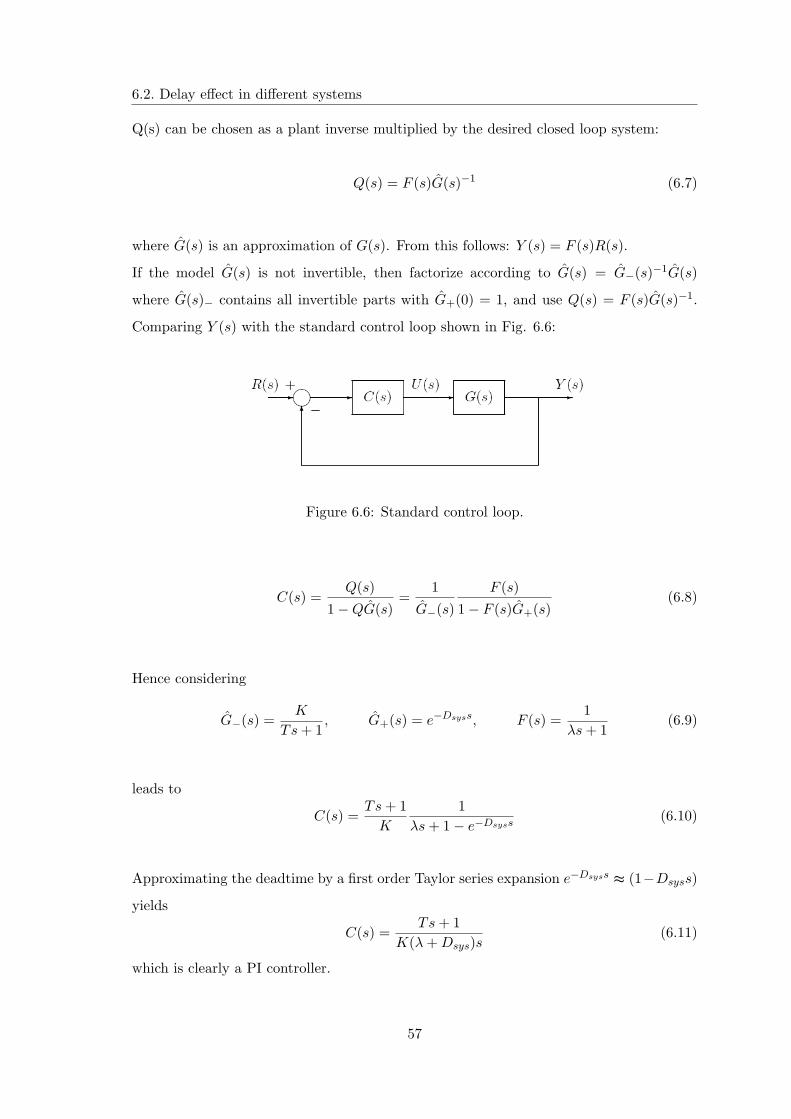
6.2. Delay effect in different systems
Both these systems can easily be controlled using a PI controller of this type
C(s) = Kc(1 +1
TIs) (6.4)
6.2.1 First-order Stable System
The first case represents a first order stable system affected by a delay Dsys:
G(s) =K
Ts + 1e−Dsyss (6.5)
The controller chosen is a PI because of its simplicity. The tuning of the PI parameters
can be done following the lambda tuning technique [9].
Figure 6.5: Internal model control structure.
This considers a closed-loop of the following form (see Fig. 6.5):
Y (s) = G(s)Q(s)R(s) (6.6)
56
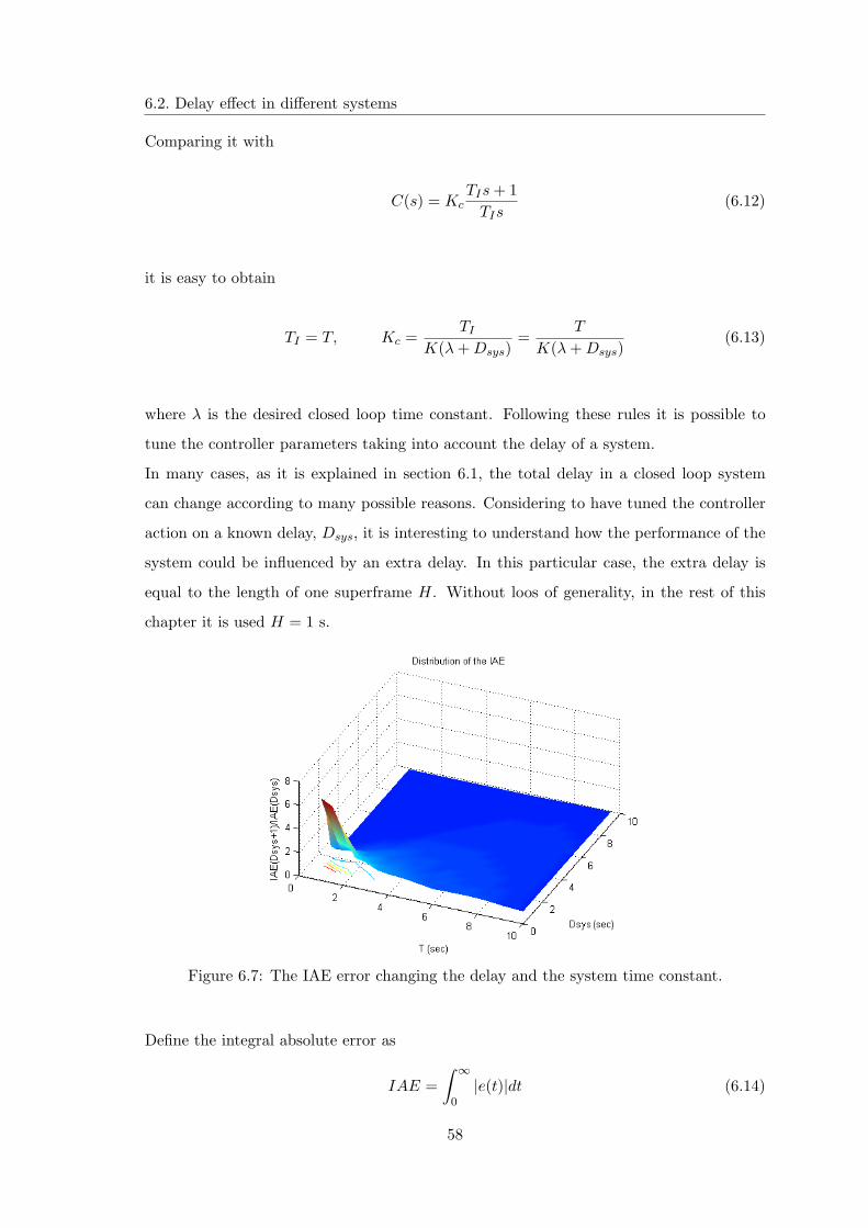
6.2. Delay effect in different systems
Q(s) can be chosen as a plant inverse multiplied by the desired closed loop system:
Q(s) = F (s)G(s)−1 (6.7)
where G(s) is an approximation of G(s). From this follows: Y (s) = F (s)R(s).
If the model G(s) is not invertible, then factorize according to G(s) = G−(s)−1G(s)
where G(s)− contains all invertible parts with G+(0) = 1, and use Q(s) = F (s)G(s)−1.
Comparing Y (s) with the standard control loop shown in Fig. 6.6:
Figure 6.6: Standard control loop.
C(s) =Q(s)
1−QG(s)=
1G−(s)
F (s)1− F (s)G+(s)
(6.8)
Hence considering
G−(s) =K
Ts + 1, G+(s) = e−Dsyss, F (s) =
1λs + 1
(6.9)
leads to
C(s) =Ts + 1
K
1λs + 1− e−Dsyss
(6.10)
Approximating the deadtime by a first order Taylor series expansion e−Dsyss ≈ (1−Dsyss)
yields
C(s) =Ts + 1
K(λ + Dsys)s(6.11)
which is clearly a PI controller.
57
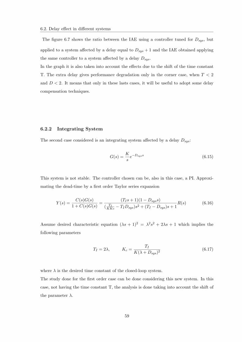
6.2. Delay effect in different systems
Comparing it with
C(s) = KcTIs + 1
TIs(6.12)
it is easy to obtain
TI = T, Kc =TI
K(λ + Dsys)=
T
K(λ + Dsys)(6.13)
where λ is the desired closed loop time constant. Following these rules it is possible to
tune the controller parameters taking into account the delay of a system.
In many cases, as it is explained in section 6.1, the total delay in a closed loop system
can change according to many possible reasons. Considering to have tuned the controller
action on a known delay, Dsys, it is interesting to understand how the performance of the
system could be influenced by an extra delay. In this particular case, the extra delay is
equal to the length of one superframe H. Without loos of generality, in the rest of this
chapter it is used H = 1 s.
Figure 6.7: The IAE error changing the delay and the system time constant.
Define the integral absolute error as
IAE =∫ ∞
0|e(t)|dt (6.14)
58
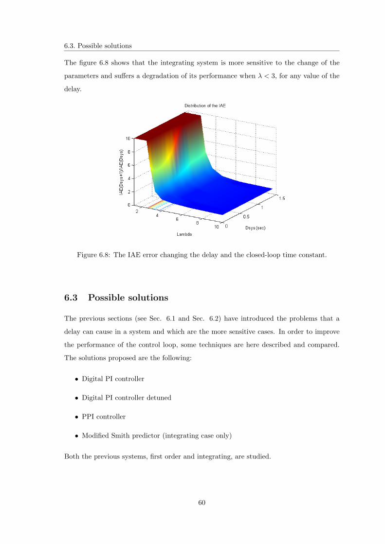
6.2. Delay effect in different systems
The figure 6.7 shows the ratio between the IAE using a controller tuned for Dsys, but
applied to a system affected by a delay equal to Dsys + 1 and the IAE obtained applying
the same controller to a system affected by a delay Dsys.
In the graph it is also taken into account the effects due to the shift of the time constant
T. The extra delay gives performance degradation only in the corner case, when T < 2
and D < 2. It means that only in these lasts cases, it will be useful to adopt some delay
compensation techniques.
6.2.2 Integrating System
The second case considered is an integrating system affected by a delay Dsys:
G(s) =K
se−Dsyss (6.15)
This system is not stable. The controller chosen can be, also in this case, a PI. Approxi-
mating the dead-time by a first order Taylor series expansion
Y (s) =C(s)G(s)
1 + C(s)G(s)=
(TIs + 1)(1−Dsyss)( TI
KKc − TIDsys)s2 + (TI −Dsys)s + 1R(s) (6.16)
Assume desired characteristic equation (λs + 1)2 = λ2s2 + 2λs + 1 which implies the
following parameters
TI = 2λ, Kc =TI
K(λ + Dsys)2(6.17)
where λ is the desired time constant of the closed-loop system.
The study done for the first order case can be done considering this new system. In this
case, not having the time constant T, the analysis is done taking into account the shift of
the parameter λ.
59
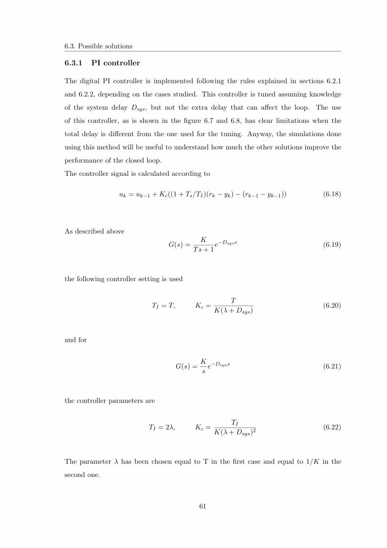
6.3. Possible solutions
The figure 6.8 shows that the integrating system is more sensitive to the change of the
parameters and suffers a degradation of its performance when λ < 3, for any value of the
delay.
Figure 6.8: The IAE error changing the delay and the closed-loop time constant.
6.3 Possible solutions
The previous sections (see Sec. 6.1 and Sec. 6.2) have introduced the problems that a
delay can cause in a system and which are the more sensitive cases. In order to improve
the performance of the control loop, some techniques are here described and compared.
The solutions proposed are the following:
• Digital PI controller
• Digital PI controller detuned
• PPI controller
• Modified Smith predictor (integrating case only)
Both the previous systems, first order and integrating, are studied.
60
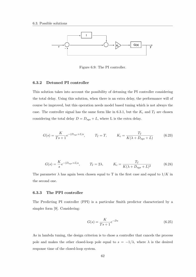
6.3. Possible solutions
6.3.1 PI controller
The digital PI controller is implemented following the rules explained in sections 6.2.1
and 6.2.2, depending on the cases studied. This controller is tuned assuming knowledge
of the system delay Dsys, but not the extra delay that can affect the loop. The use
of this controller, as is shown in the figure 6.7 and 6.8, has clear limitations when the
total delay is different from the one used for the tuning. Anyway, the simulations done
using this method will be useful to understand how much the other solutions improve the
performance of the closed loop.
The controller signal is calculated according to
uk = uk−1 + Kc((1 + Ts/TI)(rk − yk)− (rk−1 − yk−1)) (6.18)
As described above
G(s) =K
Ts + 1e−Dsyss (6.19)
the following controller setting is used
TI = T, Kc =T
K(λ + Dsys)(6.20)
and for
G(s) =K
se−Dsyss (6.21)
the controller parameters are
TI = 2λ, Kc =TI
K(λ + Dsys)2(6.22)
The parameter λ has been chosen equal to T in the first case and equal to 1/K in the
second one.
61
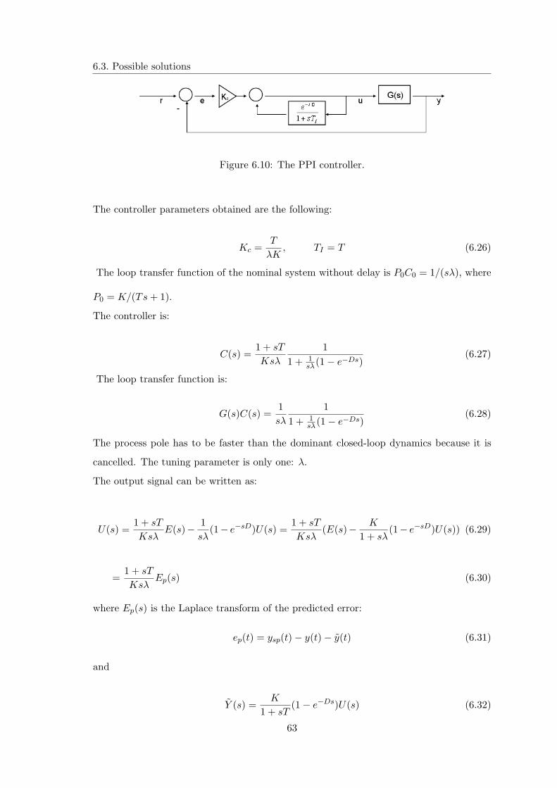
6.3. Possible solutions
Figure 6.9: The PI controller.
6.3.2 Detuned PI controller
This solution takes into account the possibility of detuning the PI controller considering
the total delay. Using this solution, when there is an extra delay, the performance will of
course be improved, but this operation needs model based tuning which is not always the
case. The controller signal has the same form like in 6.3.1, but the Kc and TI are chosen
considering the total delay D = Dsys + L, where L is the extra delay.
G(s) =K
Ts + 1e−(Dsys+L)s, TI = T, Kc =
TI
K(λ + Dsys + L)(6.23)
G(s) =K
se−(Dsys+L)s, TI = 2λ, Kc =
TI
K(λ + Dsys + L)2(6.24)
The parameter λ has again been chosen equal to T in the first case and equal to 1/K in
the second one.
6.3.3 The PPI controller
The Predicting PI controller (PPI) is a particular Smith predictor characterized by a
simpler form [9]. Considering:
G(s) =K
Ts + 1e−Ds (6.25)
As in lambda tuning, the design criterion is to chose a controller that cancels the process
pole and makes the other closed-loop pole equal to s = −1/λ, where λ is the desired
response time of the closed-loop system.
62
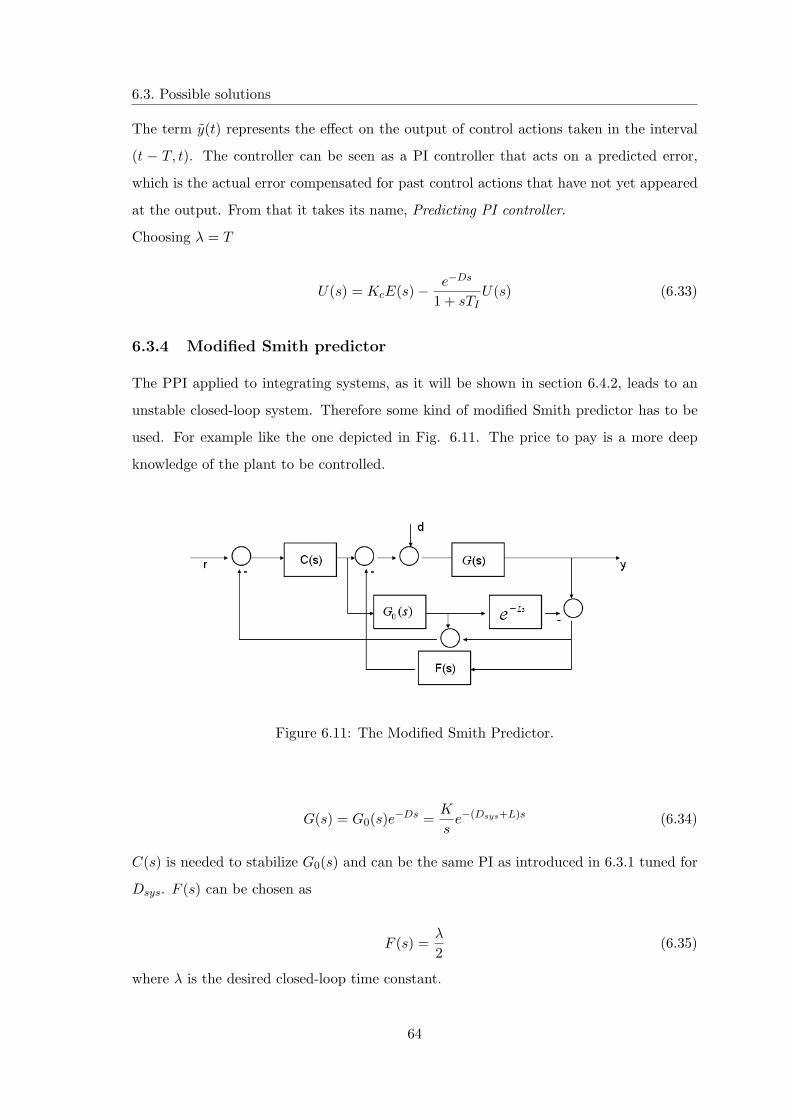
6.3. Possible solutions
Figure 6.10: The PPI controller.
The controller parameters obtained are the following:
Kc =T
λK, TI = T (6.26)
The loop transfer function of the nominal system without delay is P0C0 = 1/(sλ), where
P0 = K/(Ts + 1).
The controller is:
C(s) =1 + sT
Ksλ
11 + 1
sλ(1− e−Ds)(6.27)
The loop transfer function is:
G(s)C(s) =1sλ
11 + 1
sλ(1− e−Ds)(6.28)
The process pole has to be faster than the dominant closed-loop dynamics because it is
cancelled. The tuning parameter is only one: λ.
The output signal can be written as:
U(s) =1 + sT
KsλE(s)− 1
sλ(1− e−sD)U(s) =
1 + sT
Ksλ(E(s)− K
1 + sλ(1− e−sD)U(s)) (6.29)
=1 + sT
KsλEp(s) (6.30)
where Ep(s) is the Laplace transform of the predicted error:
ep(t) = ysp(t)− y(t)− y(t) (6.31)
and
Y (s) =K
1 + sT(1− e−Ds)U(s) (6.32)
63
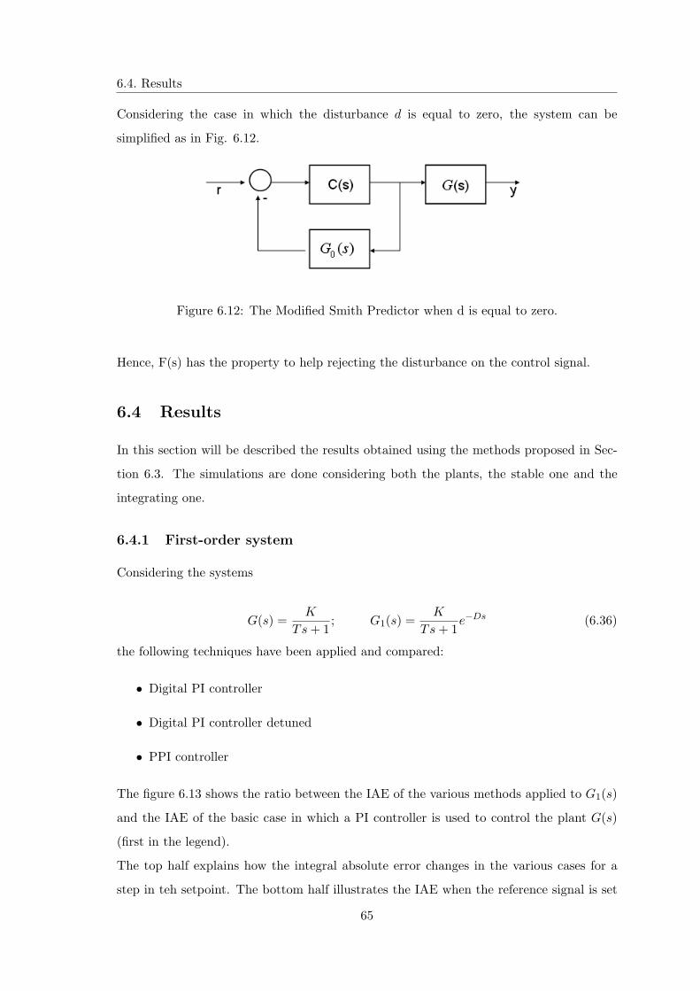
6.3. Possible solutions
The term y(t) represents the effect on the output of control actions taken in the interval
(t − T, t). The controller can be seen as a PI controller that acts on a predicted error,
which is the actual error compensated for past control actions that have not yet appeared
at the output. From that it takes its name, Predicting PI controller.
Choosing λ = T
U(s) = KcE(s)− e−Ds
1 + sTIU(s) (6.33)
6.3.4 Modified Smith predictor
The PPI applied to integrating systems, as it will be shown in section 6.4.2, leads to an
unstable closed-loop system. Therefore some kind of modified Smith predictor has to be
used. For example like the one depicted in Fig. 6.11. The price to pay is a more deep
knowledge of the plant to be controlled.
Figure 6.11: The Modified Smith Predictor.
G(s) = G0(s)e−Ds =K
se−(Dsys+L)s (6.34)
C(s) is needed to stabilize G0(s) and can be the same PI as introduced in 6.3.1 tuned for
Dsys. F (s) can be chosen as
F (s) =λ
2(6.35)
where λ is the desired closed-loop time constant.
64
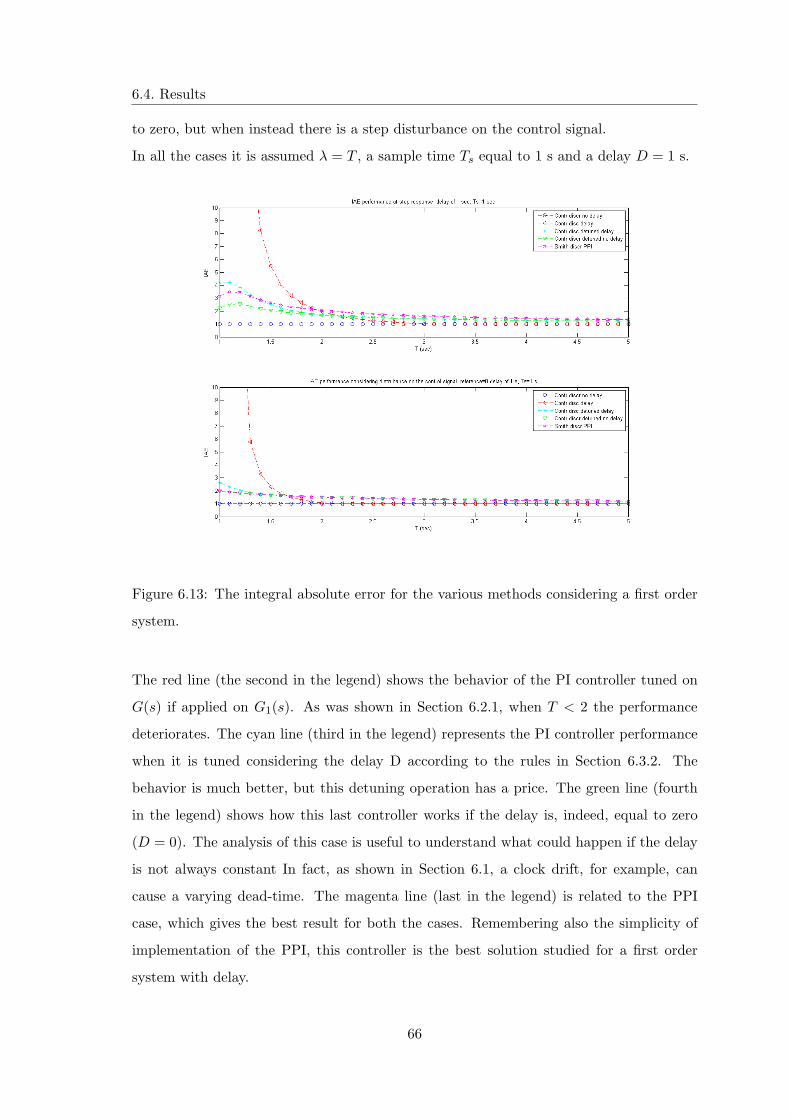
6.4. Results
Considering the case in which the disturbance d is equal to zero, the system can be
simplified as in Fig. 6.12.
Figure 6.12: The Modified Smith Predictor when d is equal to zero.
Hence, F(s) has the property to help rejecting the disturbance on the control signal.
6.4 Results
In this section will be described the results obtained using the methods proposed in Sec-
tion 6.3. The simulations are done considering both the plants, the stable one and the
integrating one.
6.4.1 First-order system
Considering the systems
G(s) =K
Ts + 1; G1(s) =
K
Ts + 1e−Ds (6.36)
the following techniques have been applied and compared:
• Digital PI controller
• Digital PI controller detuned
• PPI controller
The figure 6.13 shows the ratio between the IAE of the various methods applied to G1(s)
and the IAE of the basic case in which a PI controller is used to control the plant G(s)
(first in the legend).
The top half explains how the integral absolute error changes in the various cases for a
step in teh setpoint. The bottom half illustrates the IAE when the reference signal is set
65
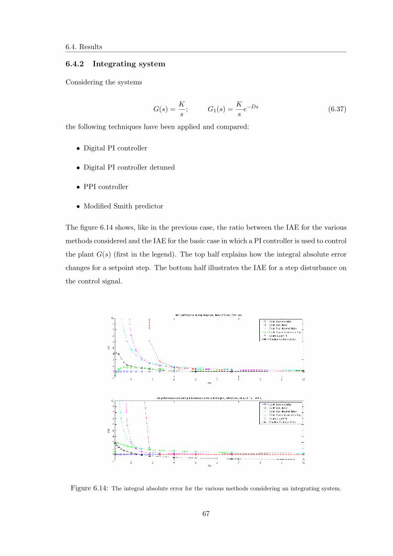
6.4. Results
to zero, but when instead there is a step disturbance on the control signal.
In all the cases it is assumed λ = T , a sample time Ts equal to 1 s and a delay D = 1 s.
Figure 6.13: The integral absolute error for the various methods considering a first order
system.
The red line (the second in the legend) shows the behavior of the PI controller tuned on
G(s) if applied on G1(s). As was shown in Section 6.2.1, when T < 2 the performance
deteriorates. The cyan line (third in the legend) represents the PI controller performance
when it is tuned considering the delay D according to the rules in Section 6.3.2. The
behavior is much better, but this detuning operation has a price. The green line (fourth
in the legend) shows how this last controller works if the delay is, indeed, equal to zero
(D = 0). The analysis of this case is useful to understand what could happen if the delay
is not always constant In fact, as shown in Section 6.1, a clock drift, for example, can
cause a varying dead-time. The magenta line (last in the legend) is related to the PPI
case, which gives the best result for both the cases. Remembering also the simplicity of
implementation of the PPI, this controller is the best solution studied for a first order
system with delay.
66
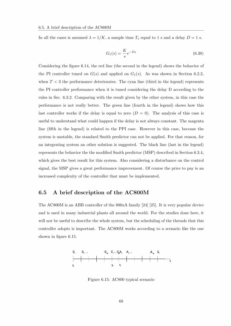
6.4. Results
6.4.2 Integrating system
Considering the systems
G(s) =K
s; G1(s) =
K
se−Ds (6.37)
the following techniques have been applied and compared:
• Digital PI controller
• Digital PI controller detuned
• PPI controller
• Modified Smith predictor
The figure 6.14 shows, like in the previous case, the ratio between the IAE for the various
methods considered and the IAE for the basic case in which a PI controller is used to control
the plant G(s) (first in the legend). The top half explains how the integral absolute error
changes for a setpoint step. The bottom half illustrates the IAE for a step disturbance on
the control signal.
Figure 6.14: The integral absolute error for the various methods considering an integrating system.
67
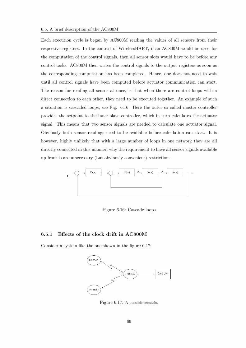
6.5. A brief description of the AC800M
In all the cases is assumed λ = 1/K, a sample time Ts equal to 1 s and a delay D = 1 s.
G1(s) =K
se−Ds (6.38)
Considering the figure 6.14, the red line (the second in the legend) shows the behavior of
the PI controller tuned on G(s) and applied on G1(s). As was shown in Section 6.2.2,
when T < 3 the performance deteriorates. The cyan line (third in the legend) represents
the PI controller performance when it is tuned considering the delay D according to the
rules in Sec. 6.3.2. Comparing with the result given by the other system, in this case the
performance is not really better. The green line (fourth in the legend) shows how this
last controller works if the delay is equal to zero (D = 0). The analysis of this case is
useful to understand what could happen if the delay is not always constant. The magenta
line (fifth in the legend) is related to the PPI case. However in this case, becouse the
system is unstable, the standard Smith predictor can not be applied. For that reason, for
an integrating system an other solution is suggested. The black line (last in the legend)
represents the behavior the the modified Smith predictor (MSP) described in Section 6.3.4,
which gives the best result for this system. Also considering a disturbance on the control
signal, the MSP gives a great performance improvement. Of course the price to pay is an
increased complexity of the controller that must be implemented.
6.5 A brief description of the AC800M
The AC800M is an ABB controller of the 800xA family [24] [25]. It is very popular device
and is used in many industrial plants all around the world. For the studies done here, it
will not be useful to describe the whole system, but the scheduling of the threads that this
controller adopts is important. The AC800M works according to a scenario like the one
shown in figure 6.15.
Figure 6.15: AC800 typical scenario
68
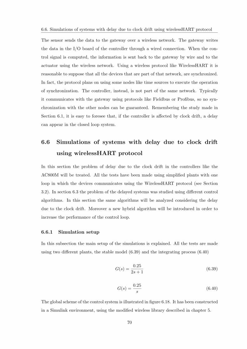
6.5. A brief description of the AC800M
Each execution cycle is began by AC800M reading the values of all sensors from their
respective registers. In the context of WirelessHART, if an AC800M would be used for
the computation of the control signals, then all sensor slots would have to be before any
control tasks. AC800M then writes the control signals to the output registers as soon as
the corresponding computation has been completed. Hence, one does not need to wait
until all control signals have been computed before actuator communication can start.
The reason for reading all sensor at once, is that when there are control loops with a
direct connection to each other, they need to be executed together. An example of such
a situation is cascaded loops, see Fig. 6.16. Here the outer so called master controller
provides the setpoint to the inner slave controller, which in turn calculates the actuator
signal. This means that two sensor signals are needed to calculate one actuator signal.
Obviously both sensor readings need to be available before calculation can start. It is
however, highly unlikely that with a large number of loops in one network they are all
directly connected in this manner, why the requirement to have all sensor signals available
up front is an unnecessary (but obviously convenient) restriction.
Figure 6.16: Cascade loops
6.5.1 Effects of the clock drift in AC800M
Consider a system like the one shown in the figure 6.17:
Figure 6.17: A possible scenario.
69
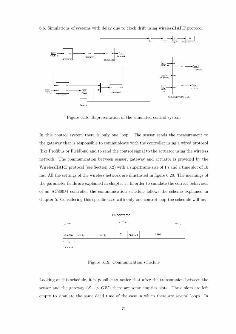
6.6. Simulations of systems with delay due to clock drift using wirelessHART protocol
The sensor sends the data to the gateway over a wireless network. The gateway writes
the data in the I/O board of the controller through a wired connection. When the con-
trol signal is computed, the information is sent back to the gateway by wire and to the
actuator using the wireless network. Using a wireless protocol like WirelessHART it is
reasonable to suppose that all the devices that are part of that network, are synchronized.
In fact, the protocol plans on using some nodes like time sources to execute the operation
of synchronization. The controller, instead, is not part of the same network. Typically
it communicates with the gateway using protocols like Fieldbus or Profibus, so no syn-
chronization with the other nodes can be guaranteed. Remembering the study made in
Section 6.1, it is easy to foresee that, if the controller is affected by clock drift, a delay
can appear in the closed loop system.
6.6 Simulations of systems with delay due to clock drift
using wirelessHART protocol
In this section the problem of delay due to the clock drift in the controllers like the
AC800M will be treated. All the tests have been made using simplified plants with one
loop in which the devices communicates using the WirelessHART protocol (see Section
3.2). In section 6.3 the problem of the delayed systems was studied using different control
algorithms. In this section the same algorithms will be analyzed considering the delay
due to the clock drift. Moreover a new hybrid algorithm will be introduced in order to
increase the performance of the control loop.
6.6.1 Simulation setup
In this subsection the main setup of the simulations is explained. All the tests are made
using two different plants, the stable model (6.39) and the integrating process (6.40)
G(s) =0.25
2s + 1(6.39)
G(s) =0.25s
(6.40)
The global scheme of the control system is illustrated in figure 6.18. It has been constructed
in a Simulink environment, using the modified wireless library described in chapter 5.
70
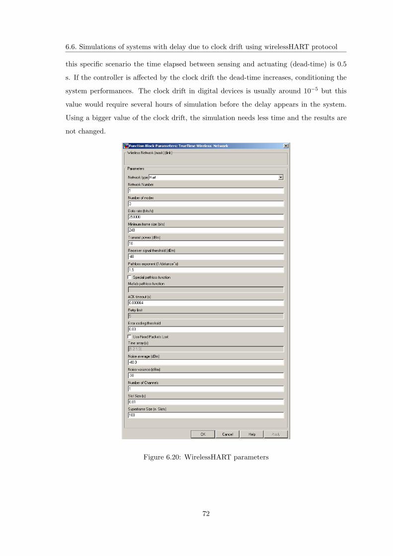
6.6. Simulations of systems with delay due to clock drift using wirelessHART protocol
Figure 6.18: Representation of the simulated control system
In this control system there is only one loop. The sensor sends the measurement to
the gateway that is responsible to communicate with the controller using a wired protocol
(like Profibus or Fieldbus) and to send the control signal to the actuator using the wireless
network. The communication between sensor, gateway and actuator is provided by the
WirelessHART protocol (see Section 3.2) with a superframe size of 1 s and a time slot of 10
ms. All the settings of the wireless network are illustrated in figure 6.20. The meanings of
the parameter fields are explained in chapter 3. In order to simulate the correct behaviour
of an AC800M controller the communication schedule follows the scheme explained in
chapter 5. Considering this specific case with only one control loop the schedule will be:
Figure 6.19: Communication schedule
Looking at this schedule, it is possible to notice that after the transmission between the
sensor and the gateway (S− > GW ) there are some empties slots. These slots are left
empty to simulate the same dead time of the case in which there are several loops. In
71
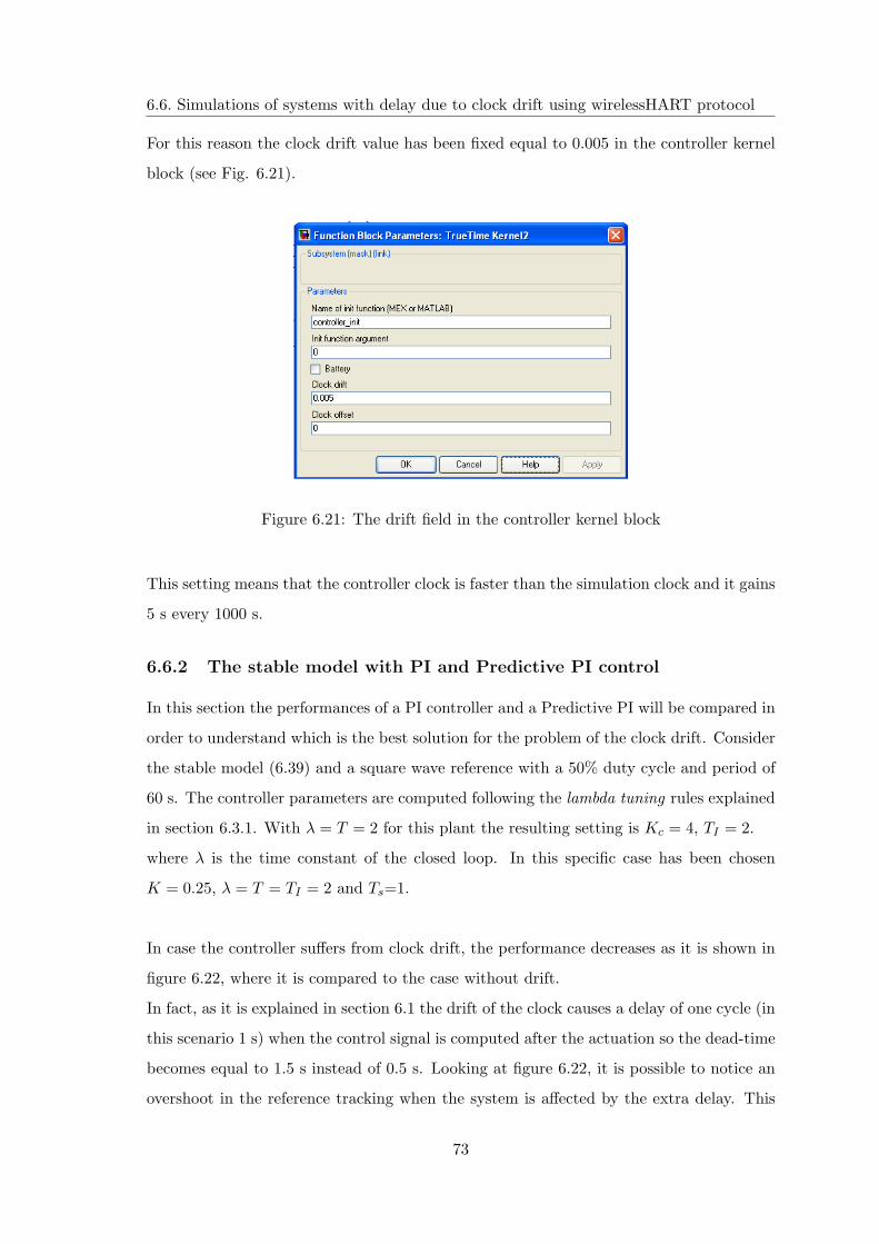
6.6. Simulations of systems with delay due to clock drift using wirelessHART protocol
this specific scenario the time elapsed between sensing and actuating (dead-time) is 0.5
s. If the controller is affected by the clock drift the dead-time increases, conditioning the
system performances. The clock drift in digital devices is usually around 10−5 but this
value would require several hours of simulation before the delay appears in the system.
Using a bigger value of the clock drift, the simulation needs less time and the results are
not changed.
Figure 6.20: WirelessHART parameters
72
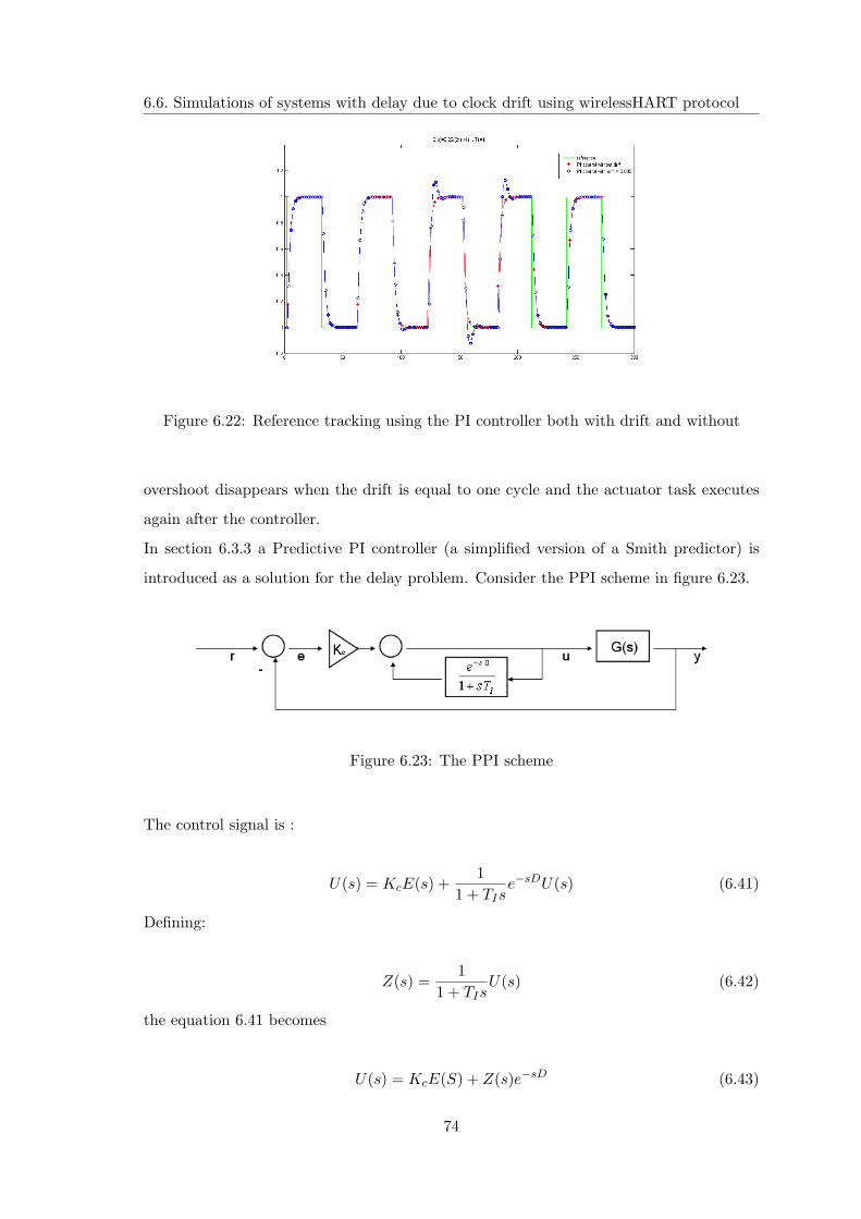
6.6. Simulations of systems with delay due to clock drift using wirelessHART protocol
For this reason the clock drift value has been fixed equal to 0.005 in the controller kernel
block (see Fig. 6.21).
Figure 6.21: The drift field in the controller kernel block
This setting means that the controller clock is faster than the simulation clock and it gains
5 s every 1000 s.
6.6.2 The stable model with PI and Predictive PI control
In this section the performances of a PI controller and a Predictive PI will be compared in
order to understand which is the best solution for the problem of the clock drift. Consider
the stable model (6.39) and a square wave reference with a 50% duty cycle and period of
60 s. The controller parameters are computed following the lambda tuning rules explained
in section 6.3.1. With λ = T = 2 for this plant the resulting setting is Kc = 4, TI = 2.
where λ is the time constant of the closed loop. In this specific case has been chosen
K = 0.25, λ = T = TI = 2 and Ts=1.
In case the controller suffers from clock drift, the performance decreases as it is shown in
figure 6.22, where it is compared to the case without drift.
In fact, as it is explained in section 6.1 the drift of the clock causes a delay of one cycle (in
this scenario 1 s) when the control signal is computed after the actuation so the dead-time
becomes equal to 1.5 s instead of 0.5 s. Looking at figure 6.22, it is possible to notice an
overshoot in the reference tracking when the system is affected by the extra delay. This
73
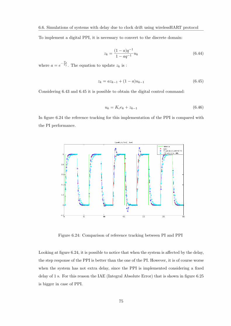
6.6. Simulations of systems with delay due to clock drift using wirelessHART protocol
Figure 6.22: Reference tracking using the PI controller both with drift and without
overshoot disappears when the drift is equal to one cycle and the actuator task executes
again after the controller.
In section 6.3.3 a Predictive PI controller (a simplified version of a Smith predictor) is
introduced as a solution for the delay problem. Consider the PPI scheme in figure 6.23.
Figure 6.23: The PPI scheme
The control signal is :
U(s) = KcE(s) +1
1 + TIse−sDU(s) (6.41)
Defining:
Z(s) =1
1 + TIsU(s) (6.42)
the equation 6.41 becomes
U(s) = KcE(S) + Z(s)e−sD (6.43)
74
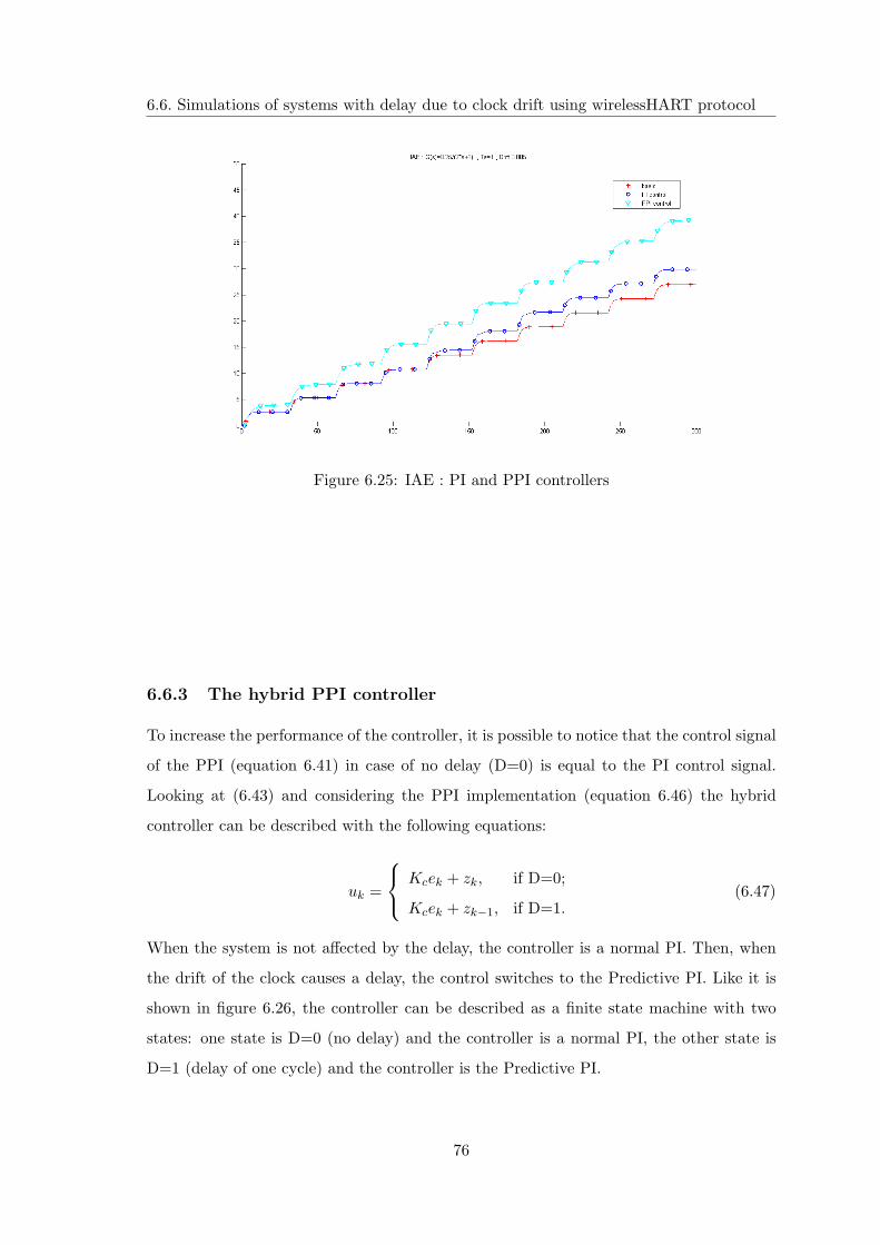
6.6. Simulations of systems with delay due to clock drift using wirelessHART protocol
To implement a digital PPI, it is necessary to convert to the discrete domain:
zk =(1− a)q−1
1− aq−1uk (6.44)
where a = e− Ts
TI . The equation to update zk is :
zk = azk−1 + (1− a)uk−1 (6.45)
Considering 6.43 and 6.45 it is possible to obtain the digital control command:
uk = Kcek + zk−1 (6.46)
In figure 6.24 the reference tracking for this implementation of the PPI is compared with
the PI performance.
Figure 6.24: Comparison of reference tracking between PI and PPI
Looking at figure 6.24, it is possible to notice that when the system is affected by the delay,
the step response of the PPI is better than the one of the PI. However, it is of course worse
when the system has not extra delay, since the PPI is implemented considering a fixed
delay of 1 s. For this reason the IAE (Integral Absolute Error) that is shown in figure 6.25
is bigger in case of PPI.
75
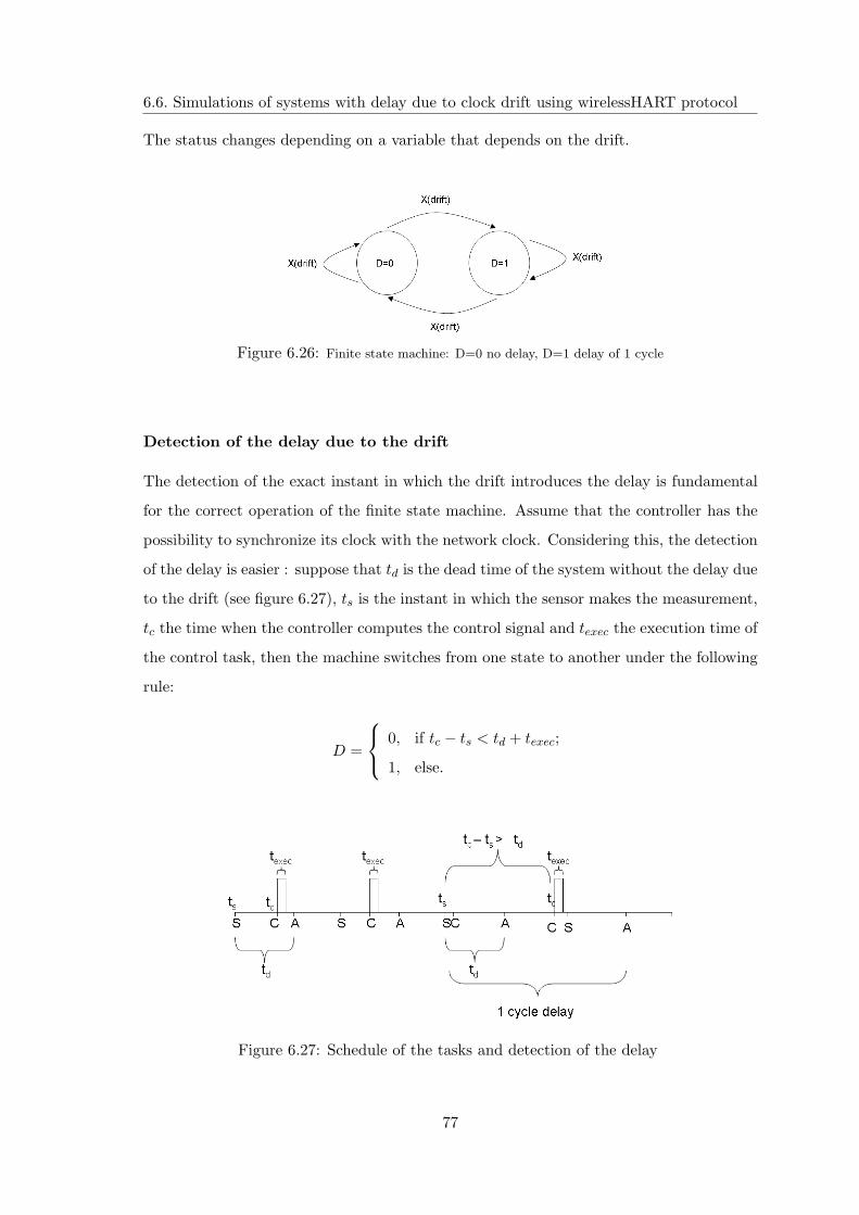
6.6. Simulations of systems with delay due to clock drift using wirelessHART protocol
Figure 6.25: IAE : PI and PPI controllers
6.6.3 The hybrid PPI controller
To increase the performance of the controller, it is possible to notice that the control signal
of the PPI (equation 6.41) in case of no delay (D=0) is equal to the PI control signal.
Looking at (6.43) and considering the PPI implementation (equation 6.46) the hybrid
controller can be described with the following equations:
uk =
Kcek + zk, if D=0;
Kcek + zk−1, if D=1.(6.47)
When the system is not affected by the delay, the controller is a normal PI. Then, when
the drift of the clock causes a delay, the control switches to the Predictive PI. Like it is
shown in figure 6.26, the controller can be described as a finite state machine with two
states: one state is D=0 (no delay) and the controller is a normal PI, the other state is
D=1 (delay of one cycle) and the controller is the Predictive PI.
76
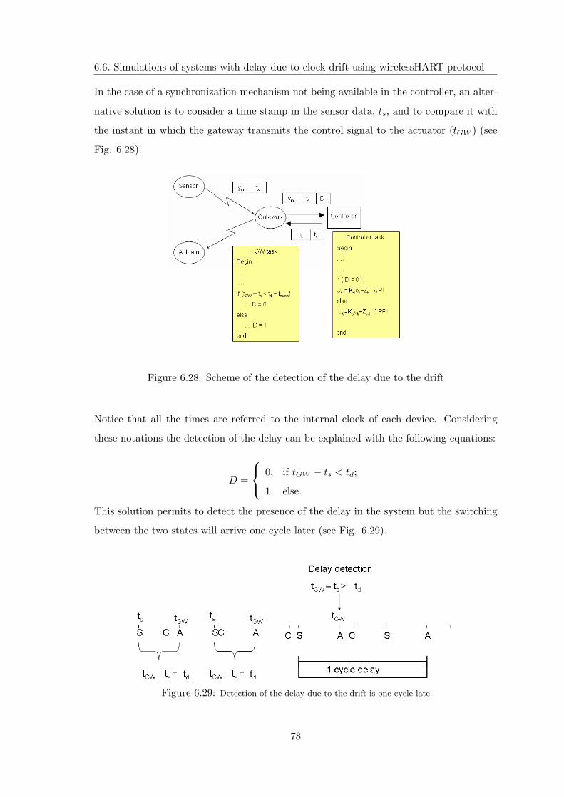
6.6. Simulations of systems with delay due to clock drift using wirelessHART protocol
The status changes depending on a variable that depends on the drift.
Figure 6.26: Finite state machine: D=0 no delay, D=1 delay of 1 cycle
Detection of the delay due to the drift
The detection of the exact instant in which the drift introduces the delay is fundamental
for the correct operation of the finite state machine. Assume that the controller has the
possibility to synchronize its clock with the network clock. Considering this, the detection
of the delay is easier : suppose that td is the dead time of the system without the delay due
to the drift (see figure 6.27), ts is the instant in which the sensor makes the measurement,
tc the time when the controller computes the control signal and texec the execution time of
the control task, then the machine switches from one state to another under the following
rule:
D =
0, if tc − ts < td + texec;
1, else.
Figure 6.27: Schedule of the tasks and detection of the delay
77
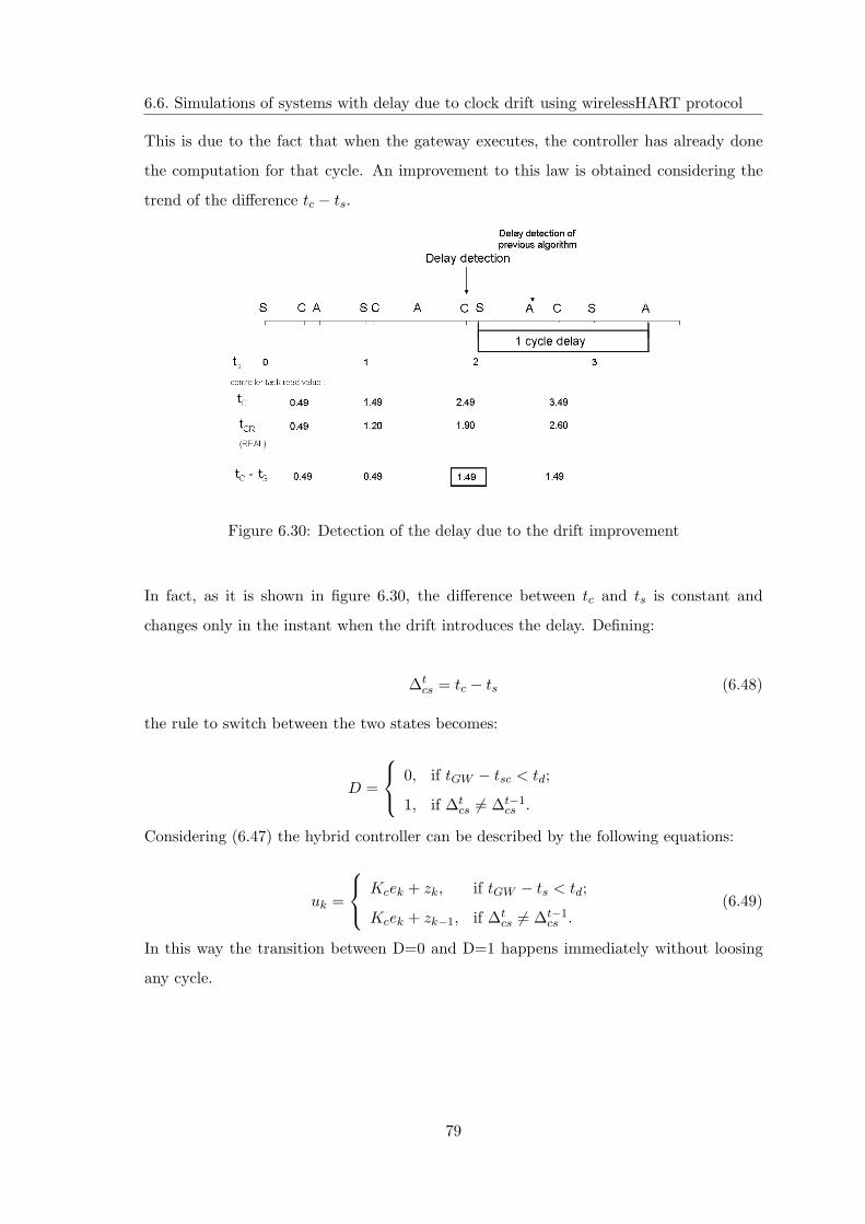
6.6. Simulations of systems with delay due to clock drift using wirelessHART protocol
In the case of a synchronization mechanism not being available in the controller, an alter-
native solution is to consider a time stamp in the sensor data, ts, and to compare it with
the instant in which the gateway transmits the control signal to the actuator (tGW ) (see
Fig. 6.28).
Figure 6.28: Scheme of the detection of the delay due to the drift
Notice that all the times are referred to the internal clock of each device. Considering
these notations the detection of the delay can be explained with the following equations:
D =
0, if tGW − ts < td;
1, else.
This solution permits to detect the presence of the delay in the system but the switching
between the two states will arrive one cycle later (see Fig. 6.29).
Figure 6.29: Detection of the delay due to the drift is one cycle late
78
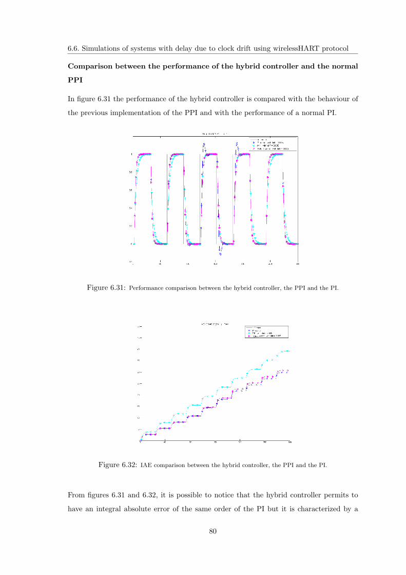
6.6. Simulations of systems with delay due to clock drift using wirelessHART protocol
This is due to the fact that when the gateway executes, the controller has already done
the computation for that cycle. An improvement to this law is obtained considering the
trend of the difference tc − ts.
Figure 6.30: Detection of the delay due to the drift improvement
In fact, as it is shown in figure 6.30, the difference between tc and ts is constant and
changes only in the instant when the drift introduces the delay. Defining:
∆tcs = tc − ts (6.48)
the rule to switch between the two states becomes:
D =
0, if tGW − tsc < td;
1, if ∆tcs 6= ∆t−1
cs .
Considering (6.47) the hybrid controller can be described by the following equations:
uk =
Kcek + zk, if tGW − ts < td;
Kcek + zk−1, if ∆tcs 6= ∆t−1
cs .(6.49)
In this way the transition between D=0 and D=1 happens immediately without loosing
any cycle.
79
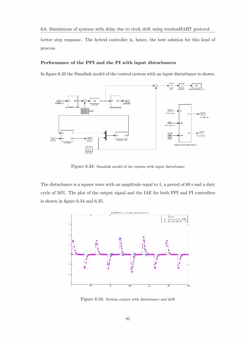
6.6. Simulations of systems with delay due to clock drift using wirelessHART protocol
Comparison between the performance of the hybrid controller and the normal
PPI
In figure 6.31 the performance of the hybrid controller is compared with the behaviour of
the previous implementation of the PPI and with the performance of a normal PI.
Figure 6.31: Performance comparison between the hybrid controller, the PPI and the PI.
Figure 6.32: IAE comparison between the hybrid controller, the PPI and the PI.
From figures 6.31 and 6.32, it is possible to notice that the hybrid controller permits to
have an integral absolute error of the same order of the PI but it is characterized by a
80
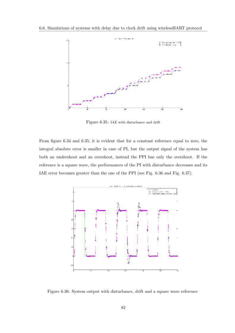
6.6. Simulations of systems with delay due to clock drift using wirelessHART protocol
better step response. The hybrid controller is, hence, the best solution for this kind of
process.
Performance of the PPI and the PI with input disturbances
In figure 6.33 the Simulink model of the control system with an input disturbance is shown.
Figure 6.33: Simulink model of the system with input disturbance
The disturbance is a square wave with an amplitude equal to 1, a period of 60 s and a duty
cycle of 50%. The plot of the output signal and the IAE for both PPI and PI controllers
is shown in figure 6.34 and 6.35.
Figure 6.34: System output with disturbance and drift
81
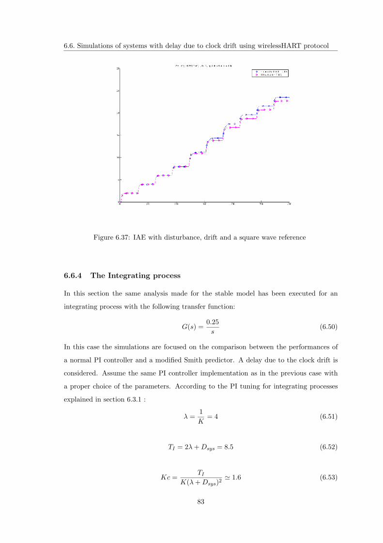
6.6. Simulations of systems with delay due to clock drift using wirelessHART protocol
Figure 6.35: IAE with disturbance and drift
From figure 6.34 and 6.35, it is evident that for a constant reference equal to zero, the
integral absolute error is smaller in case of PI, but the output signal of the system has
both an undershoot and an overshoot, instead the PPI has only the overshoot. If the
reference is a square wave, the performances of the PI with disturbance decreases and its
IAE error becomes greater than the one of the PPI (see Fig. 6.36 and Fig. 6.37).
Figure 6.36: System output with disturbance, drift and a square wave reference
82
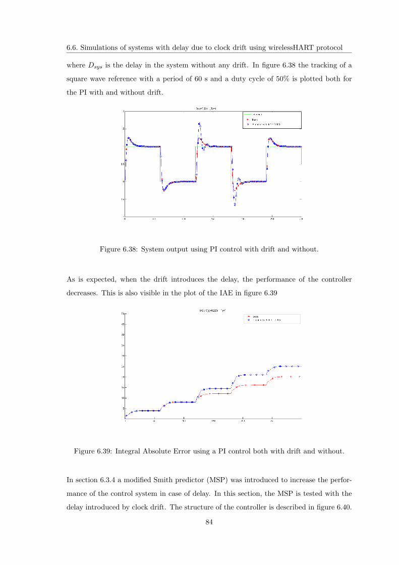
6.6. Simulations of systems with delay due to clock drift using wirelessHART protocol
Figure 6.37: IAE with disturbance, drift and a square wave reference
6.6.4 The Integrating process
In this section the same analysis made for the stable model has been executed for an
integrating process with the following transfer function:
G(s) =0.25s
(6.50)
In this case the simulations are focused on the comparison between the performances of
a normal PI controller and a modified Smith predictor. A delay due to the clock drift is
considered. Assume the same PI controller implementation as in the previous case with
a proper choice of the parameters. According to the PI tuning for integrating processes
explained in section 6.3.1 :
λ =1K
= 4 (6.51)
TI = 2λ + Dsys = 8.5 (6.52)
Kc =TI
K(λ + Dsys)2' 1.6 (6.53)
83
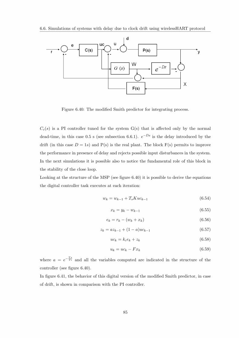
6.6. Simulations of systems with delay due to clock drift using wirelessHART protocol
where Dsys is the delay in the system without any drift. In figure 6.38 the tracking of a
square wave reference with a period of 60 s and a duty cycle of 50% is plotted both for
the PI with and without drift.
Figure 6.38: System output using PI control with drift and without.
As is expected, when the drift introduces the delay, the performance of the controller
decreases. This is also visible in the plot of the IAE in figure 6.39
Figure 6.39: Integral Absolute Error using a PI control both with drift and without.
In section 6.3.4 a modified Smith predictor (MSP) was introduced to increase the perfor-
mance of the control system in case of delay. In this section, the MSP is tested with the
delay introduced by clock drift. The structure of the controller is described in figure 6.40.
84
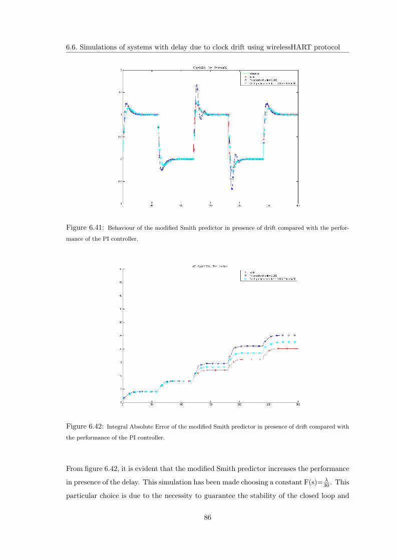
6.6. Simulations of systems with delay due to clock drift using wirelessHART protocol
Figure 6.40: The modified Smith predictor for integrating process.
Cc(s) is a PI controller tuned for the system G(s) that is affected only by the normal
dead-time, in this case 0.5 s (see subsection 6.6.1). e−Ds is the delay introduced by the
drift (in this case D = 1s) and P(s) is the real plant. The block F(s) permits to improve
the performance in presence of delay and rejects possible input disturbances in the system.
In the next simulations it is possible also to notice the fundamental role of this block in
the stability of the close loop.
Looking at the structure of the MSP (see figure 6.40) it is possible to derive the equations
the digital controller task executes at each iteration:
wk = wk−1 + TsKuck−1 (6.54)
xk = yk − wk−1 (6.55)
ek = rk − (wk + xk) (6.56)
zk = azk−1 + (1− a)uck−1 (6.57)
uck = kcek + zk (6.58)
uk = uck − Fxk (6.59)
where a = e−TsTi and all the variables computed are indicated in the structure of the
controller (see figure 6.40).
In figure 6.41, the behavior of this digital version of the modified Smith predictor, in case
of drift, is shown in comparison with the PI controller.
85
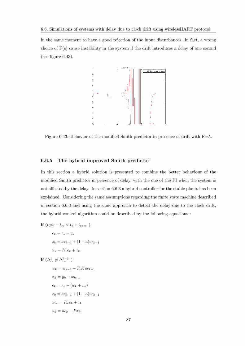
6.6. Simulations of systems with delay due to clock drift using wirelessHART protocol
Figure 6.41: Behaviour of the modified Smith predictor in presence of drift compared with the perfor-
mance of the PI controller.
Figure 6.42: Integral Absolute Error of the modified Smith predictor in presence of drift compared with
the performance of the PI controller.
From figure 6.42, it is evident that the modified Smith predictor increases the performance
in presence of the delay. This simulation has been made choosing a constant F(s)= λ30 . This
particular choice is due to the necessity to guarantee the stability of the closed loop and
86
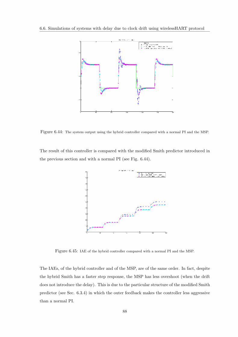
6.6. Simulations of systems with delay due to clock drift using wirelessHART protocol
in the same moment to have a good rejection of the input disturbances. In fact, a wrong
choice of F(s) cause instability in the system if the drift introduces a delay of one second
(see figure 6.43).
Figure 6.43: Behavior of the modified Smith predictor in presence of drift with F=λ.
6.6.5 The hybrid improved Smith predictor
In this section a hybrid solution is presented to combine the better behaviour of the
modified Smith predictor in presence of delay, with the one of the PI when the system is
not affected by the delay. In section 6.6.3 a hybrid controller for the stable plants has been
explained. Considering the same assumptions regarding the finite state machine described
in section 6.6.3 and using the same approach to detect the delay due to the clock drift,
the hybrid control algorithm could be described by the following equations :
if (tGW − tsc < td + texec )
ek = rk − yk
zk = azk−1 + (1− a)uck−1
uk = Kcek + zk
if (∆kcs 6= ∆k−1
cs )
wk = wk−1 + TsKuck−1
xk = yk − wk−1
ek = rk − (wk + xk)
zk = azk−1 + (1− a)uck−1
uck = Kcek + zk
uk = uck − Fxk
87
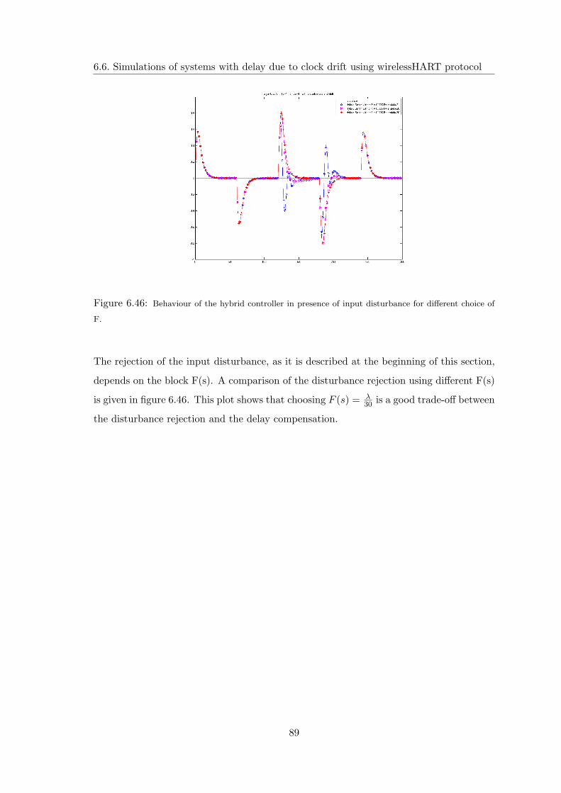
6.6. Simulations of systems with delay due to clock drift using wirelessHART protocol
Figure 6.44: The system output using the hybrid controller compared with a normal PI and the MSP.
The result of this controller is compared with the modified Smith predictor introduced in
the previous section and with a normal PI (see Fig. 6.44).
Figure 6.45: IAE of the hybrid controller compared with a normal PI and the MSP.
The IAEs, of the hybrid controller and of the MSP, are of the same order. In fact, despite
the hybrid Smith has a faster step response, the MSP has less overshoot (when the drift
does not introduce the delay). This is due to the particular structure of the modified Smith
predictor (see Sec. 6.3.4) in which the outer feedback makes the controller less aggressive
than a normal PI.
88
6.6. Simulations of systems with delay due to clock drift using wirelessHART protocol
Figure 6.46: Behaviour of the hybrid controller in presence of input disturbance for different choice of
F.
The rejection of the input disturbance, as it is described at the beginning of this section,
depends on the block F(s). A comparison of the disturbance rejection using different F(s)
is given in figure 6.46. This plot shows that choosing F (s) = λ30 is a good trade-off between
the disturbance rejection and the delay compensation.
89
Chapter 7
Conclusions
7.1 Results
The WirelessHART simulator made in this thesis work is a useful tool. It has permitted to
do all the simulations studied in this project and will give a great help in the future analysis.
The other modifications introduced in the TrueTime simulator give the possibility to have
more detailed and realistic simulations. Considering the delay compensation study, it has
been shown that the delay introduced by the clock drift of the controller is a problem.
However, also having to work with these particular processes, there are many techniques
to compensate this delay. These methods have been introduced and studied. For the first
order case, a PPI controller with a hybrid solution has shown to give the best results. It
is a very simple solution because it does not need the knowledge of all the plant model,
but only the controller parameters. In the integrating case, the situation is a bit more
complex. The PPI is not applicable and a modified Smith predictor is needed. It requires
a model of the plant that has to be controlled. It is something not always easy or cheap to
have. The results obtained for both the cases are, anyway, very positives and show that,
when a synchronization between all the devices, which is of course the preferred solution,
is not possible, the problem considered can be solved.
90
7.2. Open problems
7.2 Open problems
Future work of this project will be the study of different processes and of different delay
compensation methods. Considering the modified Smith predictor, the study of how the
stability of the closed-loop system could be affected by different values of the parameter
F is interesting. Considering, instead, the WirelessHART simulator, the implementation
of the higher levels of the WirelessHART protocol and of the various commands that
characterize it will be the aim of future studies. Also the implementation of a Network
Manager, able to modified at run-time the devices table of WirelessHART, could open
new possibility of study. It permits to modify dynamically the scheduling of the devices,
making possible a more reliable structure of the network.
91
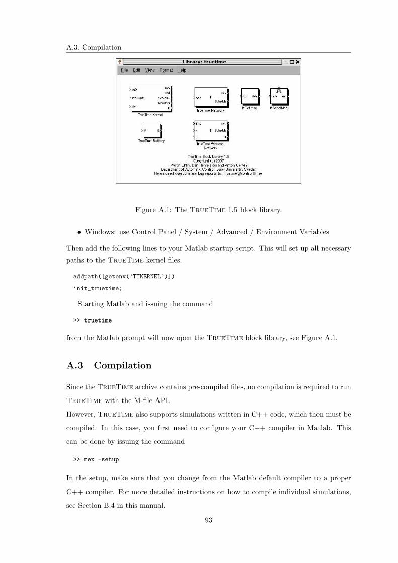
Appendix A
How to install the tool
A.1 Software Requirements
TrueTime currently supports Matlab 7.x (R14 and later) with Simulink 6.x and Matlab
6.5.1 (R13.1) with Simulink 5.1. Support for Matlab 6.1 (R12.1) with Simulink 4.1 was
dropped in TrueTime 1.3.
A C++ compiler is required to run TrueTime in the C++ version. For the Matlab ver-
sion, pre-compiled files are provided in the archive that is downloaded from the TrueTime
web site. The following compilers are currently supported (it may, of course, also work
using other compilers):
• Visual Studio C++ 7.0 (for all supported Matlab versions) for Windows
• gcc, g++ - GNU project C and C++ Compiler for LINUX and UNIX
A.2 Installation
Download and extract the compressed archive (truetime-1.5.zip), available at
http://www.control.lth.se/truetime
Extracting the file creates a truetime-1.5 directory, which will be referred to as $DIR in
the sequel.
Before starting Matlab, you must set the environment variable TTKERNEL to point to
the directory with the TrueTime kernel files, $DIR/kernel. This is typically done in the
following manner:
• Unix/Linux: export TTKERNEL=$DIR/kernel
92
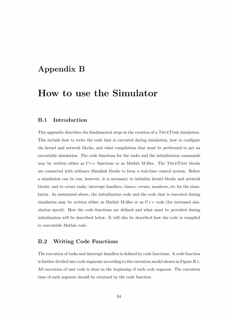
A.3. Compilation
Figure A.1: The TrueTime 1.5 block library.
• Windows: use Control Panel / System / Advanced / Environment Variables
Then add the following lines to your Matlab startup script. This will set up all necessary
paths to the TrueTime kernel files.
addpath([getenv(’TTKERNEL’)])
init_truetime;
Starting Matlab and issuing the command
>> truetime
from the Matlab prompt will now open the TrueTime block library, see Figure A.1.
A.3 Compilation
Since the TrueTime archive contains pre-compiled files, no compilation is required to run
TrueTime with the M-file API.
However, TrueTime also supports simulations written in C++ code, which then must be
compiled. In this case, you first need to configure your C++ compiler in Matlab. This
can be done by issuing the command
>> mex -setup
In the setup, make sure that you change from the Matlab default compiler to a proper
C++ compiler. For more detailed instructions on how to compile individual simulations,
see Section B.4 in this manual.
93
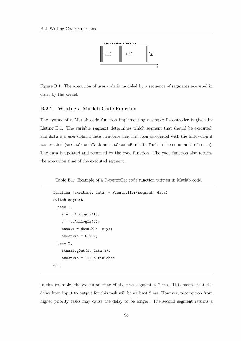
Appendix B
How to use the Simulator
B.1 Introduction
This appendix describes the fundamental steps in the creation of a TrueTime simulation.
This include how to write the code that is executed during simulation, how to configure
the kernel and network blocks, and what compilation that must be performed to get an
executable simulation. The code functions for the tasks and the initialization commands
may be written either as C++ functions or as Matlab M-files. The TrueTime blocks
are connected with ordinary Simulink blocks to form a real-time control system. Before
a simulation can be run, however, it is necessary to initialize kernel blocks and network
blocks, and to create tasks, interrupt handlers, timers, events, monitors, etc for the simu-
lation. As mentioned above, the initialization code and the code that is executed during
simulation may be written either as Matlab M-files or as C++ code (for increased sim-
ulation speed). How the code functions are defined and what must be provided during
initialization will be described below. It will also be described how the code is compiled
to executable Matlab code.
B.2 Writing Code Functions
The execution of tasks and interrupt handlers is defined by code functions. A code function
is further divided into code segments according to the execution model shown in Figure B.1.
All execution of user code is done in the beginning of each code segment. The execution
time of each segment should be returned by the code function.
94
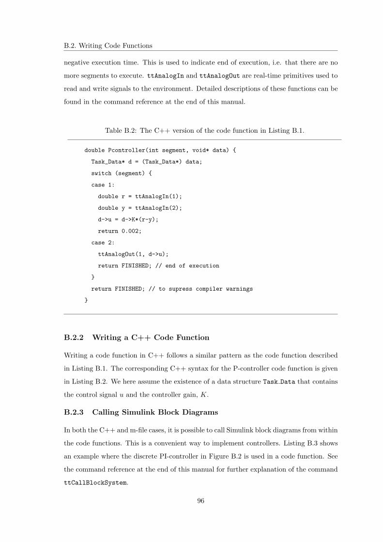
B.2. Writing Code Functions
Figure B.1: The execution of user code is modeled by a sequence of segments executed in
order by the kernel.
B.2.1 Writing a Matlab Code Function
The syntax of a Matlab code function implementing a simple P-controller is given by
Listing B.1. The variable segment determines which segment that should be executed,
and data is a user-defined data structure that has been associated with the task when it
was created (see ttCreateTask and ttCreatePeriodicTask in the command reference).
The data is updated and returned by the code function. The code function also returns
the execution time of the executed segment.
Table B.1: Example of a P-controller code function written in Matlab code.
function [exectime, data] = Pcontroller(segment, data)
switch segment,
case 1,
r = ttAnalogIn(1);
y = ttAnalogIn(2);
data.u = data.K * (r-y);
exectime = 0.002;
case 2,
ttAnalogOut(1, data.u);
exectime = -1; % finished
end
In this example, the execution time of the first segment is 2 ms. This means that the
delay from input to output for this task will be at least 2 ms. However, preemption from
higher priority tasks may cause the delay to be longer. The second segment returns a
95
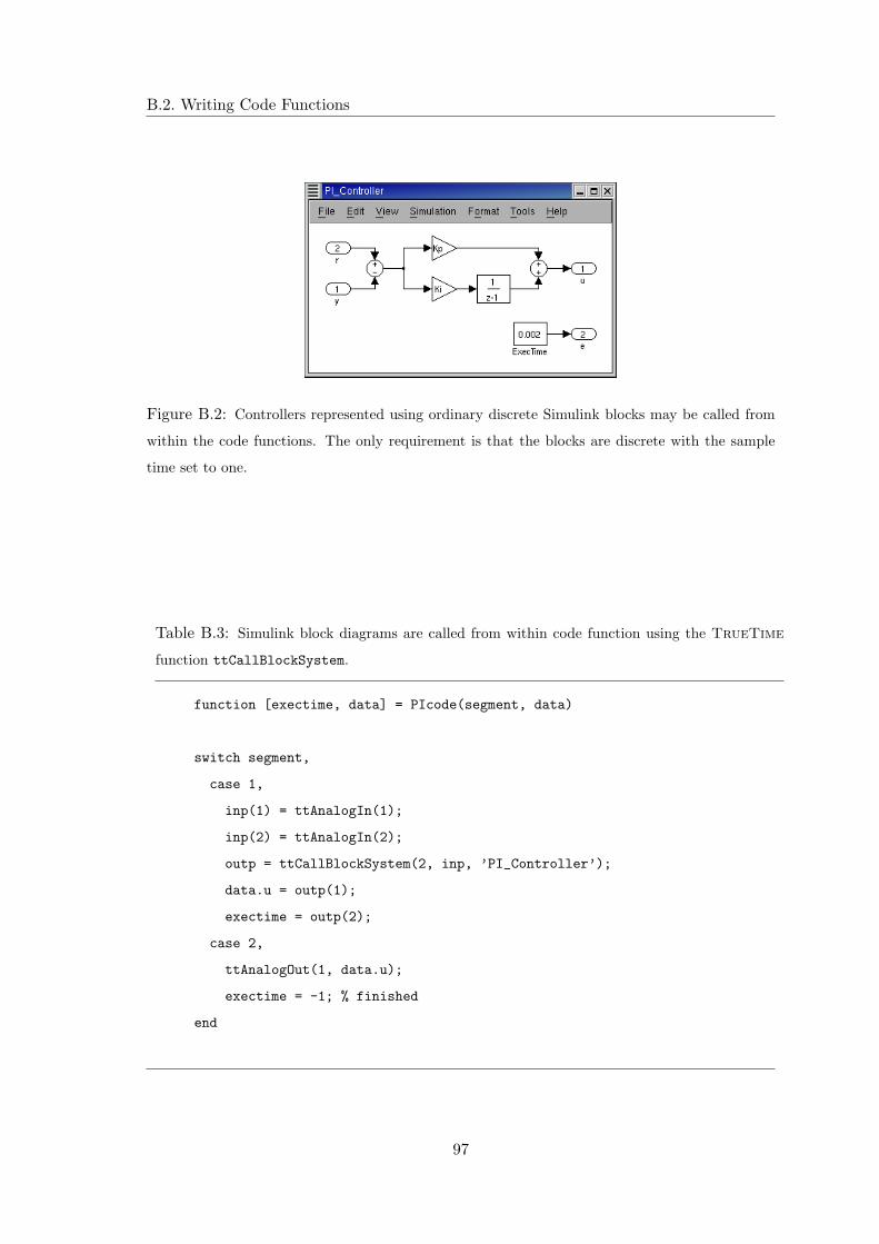
B.2. Writing Code Functions
negative execution time. This is used to indicate end of execution, i.e. that there are no
more segments to execute. ttAnalogIn and ttAnalogOut are real-time primitives used to
read and write signals to the environment. Detailed descriptions of these functions can be
found in the command reference at the end of this manual.
Table B.2: The C++ version of the code function in Listing B.1.
double Pcontroller(int segment, void* data) {
Task_Data* d = (Task_Data*) data;
switch (segment) {
case 1:
double r = ttAnalogIn(1);
double y = ttAnalogIn(2);
d->u = d->K*(r-y);
return 0.002;
case 2:
ttAnalogOut(1, d->u);
return FINISHED; // end of execution
}
return FINISHED; // to supress compiler warnings
}
B.2.2 Writing a C++ Code Function
Writing a code function in C++ follows a similar pattern as the code function described
in Listing B.1. The corresponding C++ syntax for the P-controller code function is given
in Listing B.2. We here assume the existence of a data structure Task Data that contains
the control signal u and the controller gain, K.
B.2.3 Calling Simulink Block Diagrams
In both the C++ and m-file cases, it is possible to call Simulink block diagrams from within
the code functions. This is a convenient way to implement controllers. Listing B.3 shows
an example where the discrete PI-controller in Figure B.2 is used in a code function. See
the command reference at the end of this manual for further explanation of the command
ttCallBlockSystem.
96
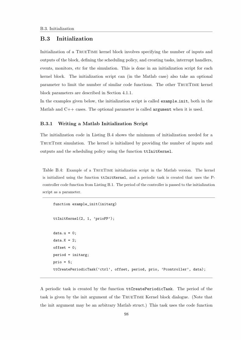
B.2. Writing Code Functions
Figure B.2: Controllers represented using ordinary discrete Simulink blocks may be called from
within the code functions. The only requirement is that the blocks are discrete with the sample
time set to one.
Table B.3: Simulink block diagrams are called from within code function using the TrueTime
function ttCallBlockSystem.
function [exectime, data] = PIcode(segment, data)
switch segment,
case 1,
inp(1) = ttAnalogIn(1);
inp(2) = ttAnalogIn(2);
outp = ttCallBlockSystem(2, inp, ’PI_Controller’);
data.u = outp(1);
exectime = outp(2);
case 2,
ttAnalogOut(1, data.u);
exectime = -1; % finished
end
97
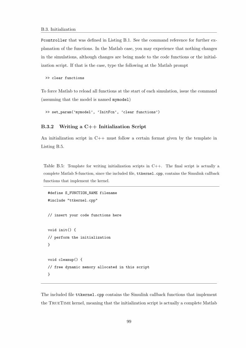
B.3. Initialization
B.3 Initialization
Initialization of a TrueTime kernel block involves specifying the number of inputs and
outputs of the block, defining the scheduling policy, and creating tasks, interrupt handlers,
events, monitors, etc for the simulation. This is done in an initialization script for each
kernel block. The initialization script can (in the Matlab case) also take an optional
parameter to limit the number of similar code functions. The other TrueTime kernel
block parameters are described in Section 4.1.1.
In the examples given below, the initialization script is called example init, both in the
Matlab and C++ cases. The optional parameter is called argument when it is used.
B.3.1 Writing a Matlab Initialization Script
The initialization code in Listing B.4 shows the minimum of initialization needed for a
TrueTime simulation. The kernel is initialized by providing the number of inputs and
outputs and the scheduling policy using the function ttInitKernel.
Table B.4: Example of a TrueTime initialization script in the Matlab version. The kernel
is initialized using the function ttInitKernel, and a periodic task is created that uses the P-
controller code function from Listing B.1. The period of the controller is passed to the initialization
script as a parameter.
function example_init(initarg)
ttInitKernel(2, 1, ’prioFP’);
data.u = 0;
data.K = 2;
offset = 0;
period = initarg;
prio = 5;
ttCreatePeriodicTask(’ctrl’, offset, period, prio, ’Pcontroller’, data);
A periodic task is created by the function ttCreatePeriodicTask. The period of the
task is given by the init argument of the TrueTime Kernel block dialogue. (Note that
the init argument may be an arbitrary Matlab struct.) This task uses the code function
98
B.3. Initialization
Pcontroller that was defined in Listing B.1. See the command reference for further ex-
planation of the functions. In the Matlab case, you may experience that nothing changes
in the simulations, although changes are being made to the code functions or the initial-
ization script. If that is the case, type the following at the Matlab prompt
>> clear functions
To force Matlab to reload all functions at the start of each simulation, issue the command
(assuming that the model is named mymodel)
>> set_param(’mymodel’, ’InitFcn’, ’clear functions’)
B.3.2 Writing a C++ Initialization Script
An initialization script in C++ must follow a certain format given by the template in
Listing B.5.
Table B.5: Template for writing initialization scripts in C++. The final script is actually a
complete Matlab S-function, since the included file, ttkernel.cpp, contains the Simulink callback
functions that implement the kernel.
#define S_FUNCTION_NAME filename
#include "ttkernel.cpp"
// insert your code functions here
void init() {
// perform the initialization
}
void cleanup() {
// free dynamic memory allocated in this script
}
The included file ttkernel.cpp contains the Simulink callback functions that implement
the TrueTime kernel, meaning that the initialization script is actually a complete Matlab
99
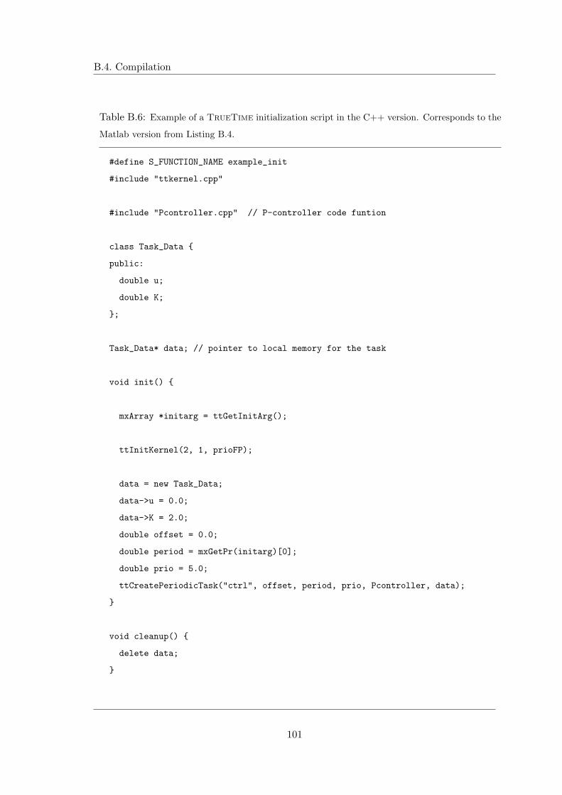
B.4. Compilation
S-function. filename should be the name of the source file, e.g. if the source file is called
example init.cpp, S FUNCTION NAME should be defined to example init.
The init()-function is called at the start of simulation (from the Simulink callback func-
tion mdlInitializeSizes), and it is here all initialization should be performed. Any dy-
namic memory allocated from the init()-function can be deallocated from the cleanup()-
function, which is called at the end of simulation. The initial argument supplied in the
TrueTime Kernel block dialogue can be retrieved using the function ttGetInitArg. The
C++ version of the Matlab initialization script of Listing B.4 is given in Listing B.6.
B.4 Compilation
Compilation requires that a proper C++ compiler has been configured in Matlab as de-
scribed in Section A.3. If needed, the TrueTime kernel may be re-compiled by issuing
the command
>> make_truetime
from the Matlab prompt. This script compiles the kernel and network S-functions and the
MEX-files for the TrueTime primitives.
In the C++ case, the initialization script (example init.cpp in the example from the
previous section) must be compiled to produce a Matlab MEX-file for the simulation.
This is done by the command
>> ttmex example_init.cpp
The initialization file needs to be recompiled each time changes are made to the code
functions or to the initialization functions.
Note: The ttmex command is the same as the ordinary mex command but includes
the path to the kernel files (ttkernel.cpp) automatically.
100
B.4. Compilation
Table B.6: Example of a TrueTime initialization script in the C++ version. Corresponds to the
Matlab version from Listing B.4.
#define S_FUNCTION_NAME example_init
#include "ttkernel.cpp"
#include "Pcontroller.cpp" // P-controller code funtion
class Task_Data {
public:
double u;
double K;
};
Task_Data* data; // pointer to local memory for the task
void init() {
mxArray *initarg = ttGetInitArg();
ttInitKernel(2, 1, prioFP);
data = new Task_Data;
data->u = 0.0;
data->K = 2.0;
double offset = 0.0;
double period = mxGetPr(initarg)[0];
double prio = 5.0;
ttCreatePeriodicTask("ctrl", offset, period, prio, Pcontroller, data);
}
void cleanup() {
delete data;
}
101
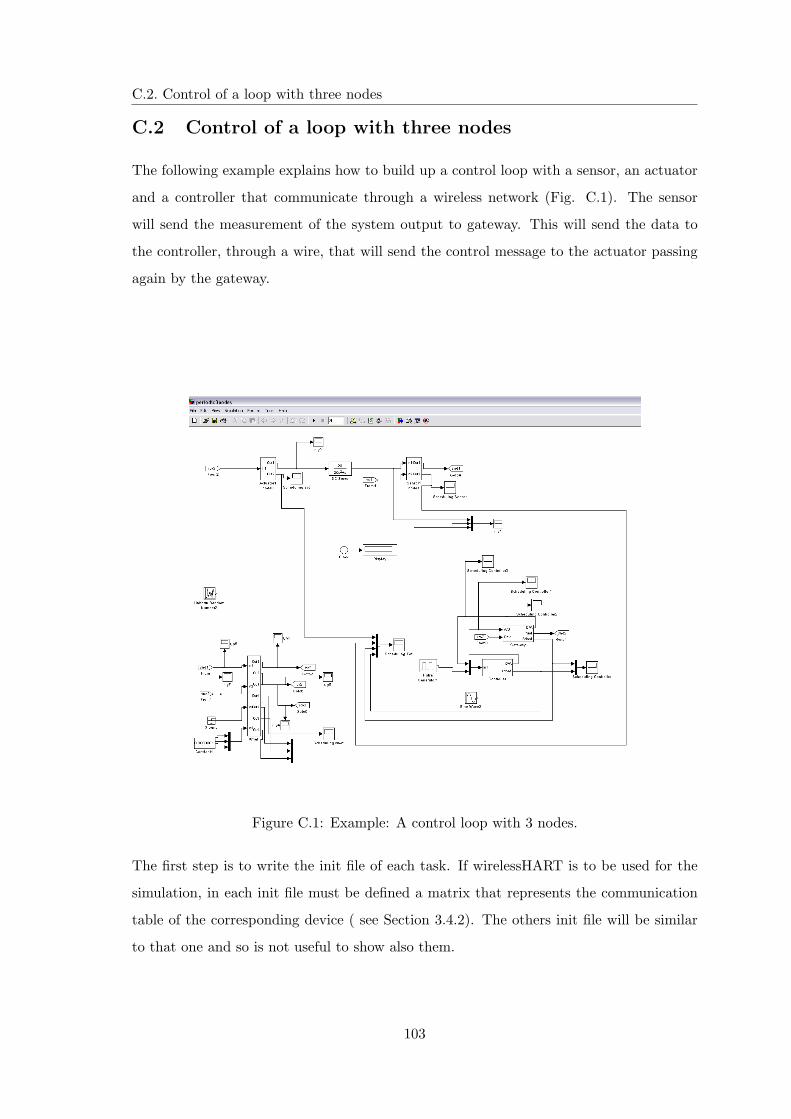
Appendix C
Examples
C.1 Introduction
This appendix presents some examples of different control loops that can be tested with
TrueTime and its new functions. In the first example will be described a simple loop in
which a system is controlled using a sensor, an actuator and controller that communicate
through a wireless network. The second shows how to control two different loops using
sensors, actuators and a controller with wirelessHART, using once shared slots and once
multi-hop strategy. The last example introduces a simple strategy to compensate the
packets loss problem. More examples are described in [5].
102
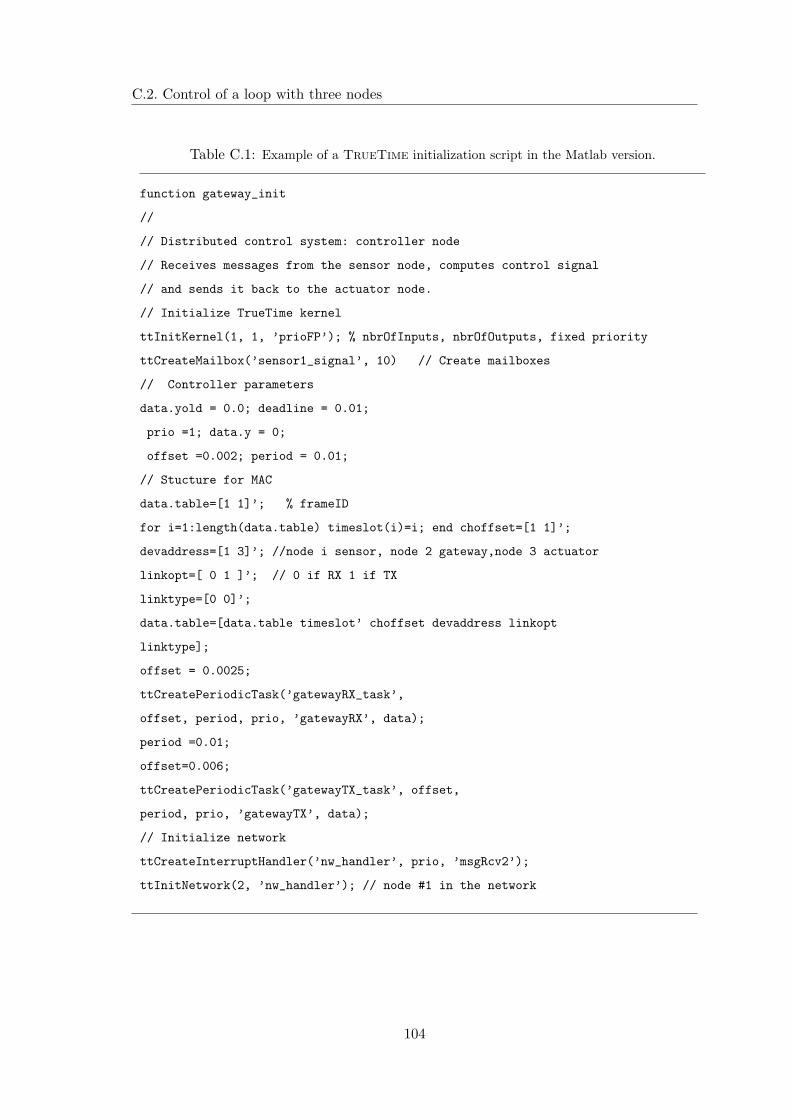
C.2. Control of a loop with three nodes
C.2 Control of a loop with three nodes
The following example explains how to build up a control loop with a sensor, an actuator
and a controller that communicate through a wireless network (Fig. C.1). The sensor
will send the measurement of the system output to gateway. This will send the data to
the controller, through a wire, that will send the control message to the actuator passing
again by the gateway.
Figure C.1: Example: A control loop with 3 nodes.
The first step is to write the init file of each task. If wirelessHART is to be used for the
simulation, in each init file must be defined a matrix that represents the communication
table of the corresponding device ( see Section 3.4.2). The others init file will be similar
to that one and so is not useful to show also them.
103
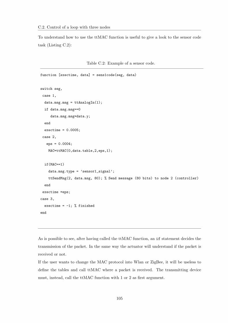
C.2. Control of a loop with three nodes
Table C.1: Example of a TrueTime initialization script in the Matlab version.
function gateway_init
//
// Distributed control system: controller node
// Receives messages from the sensor node, computes control signal
// and sends it back to the actuator node.
// Initialize TrueTime kernel
ttInitKernel(1, 1, ’prioFP’); % nbrOfInputs, nbrOfOutputs, fixed priority
ttCreateMailbox(’sensor1_signal’, 10) // Create mailboxes
// Controller parameters
data.yold = 0.0; deadline = 0.01;
prio =1; data.y = 0;
offset =0.002; period = 0.01;
// Stucture for MAC
data.table=[1 1]’; % frameID
for i=1:length(data.table) timeslot(i)=i; end choffset=[1 1]’;
devaddress=[1 3]’; //node i sensor, node 2 gateway,node 3 actuator
linkopt=[ 0 1 ]’; // 0 if RX 1 if TX
linktype=[0 0]’;
data.table=[data.table timeslot’ choffset devaddress linkopt
linktype];
offset = 0.0025;
ttCreatePeriodicTask(’gatewayRX_task’,
offset, period, prio, ’gatewayRX’, data);
period =0.01;
offset=0.006;
ttCreatePeriodicTask(’gatewayTX_task’, offset,
period, prio, ’gatewayTX’, data);
// Initialize network
ttCreateInterruptHandler(’nw_handler’, prio, ’msgRcv2’);
ttInitNetwork(2, ’nw_handler’); // node #1 in the network
104
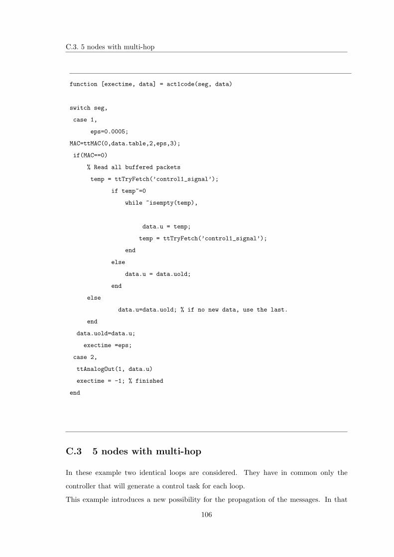
C.2. Control of a loop with three nodes
To understand how to use the ttMAC function is useful to give a look to the sensor code
task (Listing C.2):
Table C.2: Example of a sensor code.
function [exectime, data] = sens1code(seg, data)
switch seg,
case 1,
data.msg.msg = ttAnalogIn(1);
if data.msg.msg==0
data.msg.msg=data.y;
end
exectime = 0.0005;
case 2,
eps = 0.0004;
MAC=ttMAC(0,data.table,2,eps,1);
if(MAC==1)
data.msg.type = ’sensor1_signal’;
ttSendMsg(2, data.msg, 80); % Send message (80 bits) to node 2 (controller)
end
exectime =eps;
case 3,
exectime = -1; % finished
end
As is possible to see, after having called the ttMAC function, an if statement decides the
transmission of the packet. In the same way the actuator will understand if the packet is
received or not.
If the user wants to change the MAC protocol into Wlan or ZigBee, it will be useless to
define the tables and call ttMAC where a packet is received. The transmitting device
must, instead, call the ttMAC function with 1 or 2 as first argument.
105
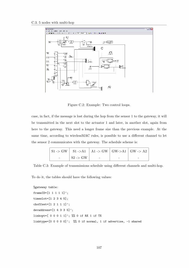
C.3. 5 nodes with multi-hop
function [exectime, data] = act1code(seg, data)
switch seg,
case 1,
eps=0.0005;
MAC=ttMAC(0,data.table,2,eps,3);
if(MAC==0)
% Read all buffered packets
temp = ttTryFetch(’control1_signal’);
if temp~=0
while ~isempty(temp),
data.u = temp;
temp = ttTryFetch(’control1_signal’);
end
else
data.u = data.uold;
end
else
data.u=data.uold; % if no new data, use the last.
end
data.uold=data.u;
exectime =eps;
case 2,
ttAnalogOut(1, data.u)
exectime = -1; % finished
end
C.3 5 nodes with multi-hop
In these example two identical loops are considered. They have in common only the
controller that will generate a control task for each loop.
This example introduces a new possibility for the propagation of the messages. In that
106
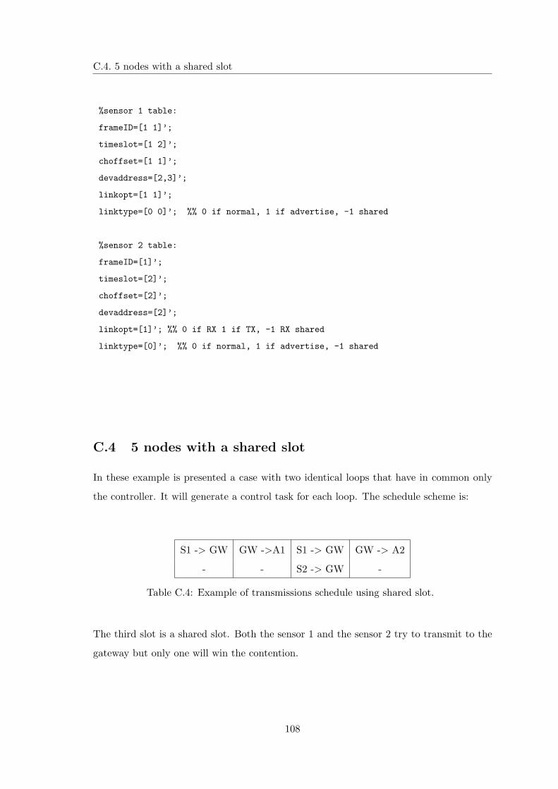
C.3. 5 nodes with multi-hop
Figure C.2: Example: Two control loops.
case, in fact, if the message is lost during the hop from the sensor 1 to the gateway, it will
be transmitted in the next slot to the actuator 1 and later, in another slot, again from
here to the gateway. This need a longer frame size than the previous example. At the
same time, according to wirelessMAC rules, is possible to use a different channel to let
the sensor 2 communicates with the gateway. The schedule scheme is:
S1 -> GW S1 ->A1 A1 -> GW GW->A1 GW -> A2
- S2 -> GW - - -
Table C.3: Example of transmissions schedule using different channels and multi-hop.
To do it, the tables should have the following values:
%gateway table:
frameID=[1 1 1 1 1]’;
timeslot=[1 2 3 4 5];
choffset=[1 2 1 1 1]’;
devaddress=[1 4 3 3 5]’;
linkopt=[ 0 0 0 1 1]’; %% 0 if RX 1 if TX
linktype=[0 0 0 0 0]’; %% 0 if normal, 1 if advertise, -1 shared
107
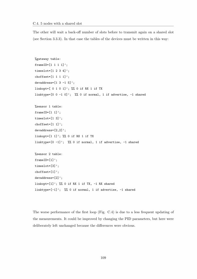
C.4. 5 nodes with a shared slot
%sensor 1 table:
frameID=[1 1]’;
timeslot=[1 2]’;
choffset=[1 1]’;
devaddress=[2,3]’;
linkopt=[1 1]’;
linktype=[0 0]’; %% 0 if normal, 1 if advertise, -1 shared
%sensor 2 table:
frameID=[1]’;
timeslot=[2]’;
choffset=[2]’;
devaddress=[2]’;
linkopt=[1]’; %% 0 if RX 1 if TX, -1 RX shared
linktype=[0]’; %% 0 if normal, 1 if advertise, -1 shared
C.4 5 nodes with a shared slot
In these example is presented a case with two identical loops that have in common only
the controller. It will generate a control task for each loop. The schedule scheme is:
S1 -> GW GW ->A1 S1 -> GW GW -> A2
- - S2 -> GW -
Table C.4: Example of transmissions schedule using shared slot.
The third slot is a shared slot. Both the sensor 1 and the sensor 2 try to transmit to the
gateway but only one will win the contention.
108
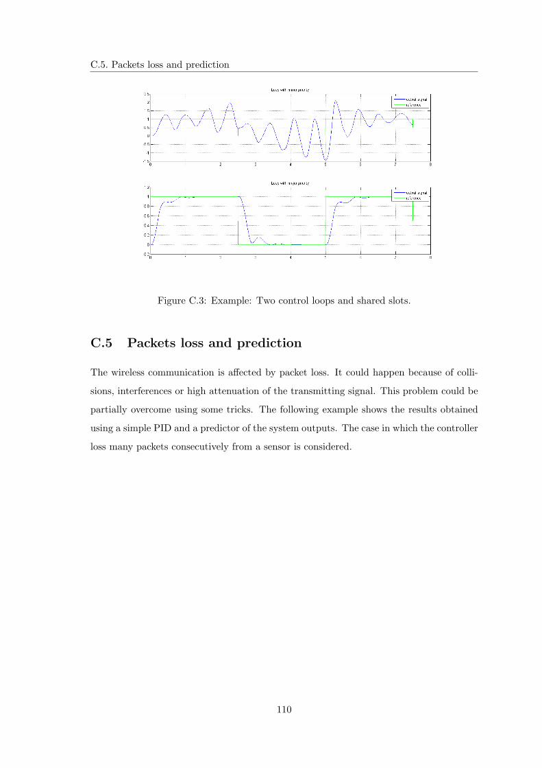
C.4. 5 nodes with a shared slot
The other will wait a back-off number of slots before to transmit again on a shared slot
(see Section 3.3.3). In that case the tables of the devices must be written in this way:
%gateway table:
frameID=[1 1 1 1]’;
timeslot=[1 2 3 4]’;
choffset=[1 1 1 1]’;
devaddress=[1 3 -1 5]’;
linkopt=[ 0 1 0 1]’; %% 0 if RX 1 if TX
linktype=[0 0 -1 0]’; %% 0 if normal, 1 if advertise, -1 shared
%sensor 1 table:
frameID=[1 1]’;
timeslot=[1 3]’;
choffset=[1 1]’;
devaddress=[2,2]’;
linkopt=[1 1]’; %% 0 if RX 1 if TX
linktype=[0 -1]’; %% 0 if normal, 1 if advertise, -1 shared
%sensor 2 table:
frameID=[1]’;
timeslot=[3]’;
choffset=[1]’;
devaddress=[2]’;
linkopt=[1]’; %% 0 if RX 1 if TX, -1 RX shared
linktype=[-1]’; %% 0 if normal, 1 if advertise, -1 shared
The worse performance of the first loop (Fig. C.4) is due to a less frequent updating of
the measurements. It could be improved by changing the PID parameters, but here were
deliberately left unchanged because the differences were obvious.
109
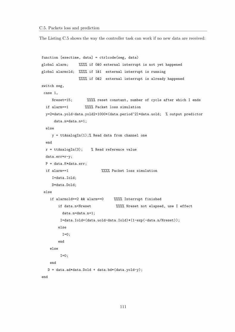
C.5. Packets loss and prediction
Figure C.3: Example: Two control loops and shared slots.
C.5 Packets loss and prediction
The wireless communication is affected by packet loss. It could happen because of colli-
sions, interferences or high attenuation of the transmitting signal. This problem could be
partially overcome using some tricks. The following example shows the results obtained
using a simple PID and a predictor of the system outputs. The case in which the controller
loss many packets consecutively from a sensor is considered.
110
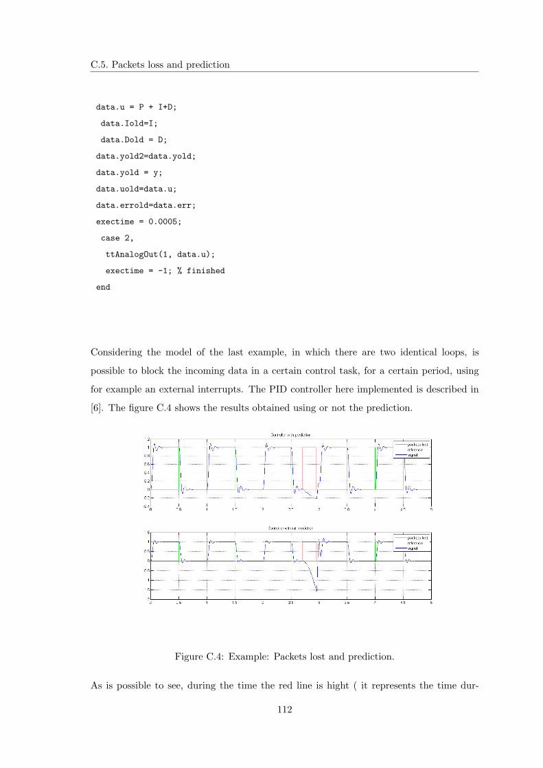
C.5. Packets loss and prediction
The Listing C.5 shows the way the controller task can work if no new data are received:
function [exectime, data] = ctrlcode(seg, data)
global alarm; %%%% if 0&0 external interrupt is not yet happened
global alarmold; %%%% if 1&1 external interrupt is running
%%%% if 0&2 external interrupt is already happened
switch seg,
case 1,
Nreset=15; %%%% reset constant, number of cycle after which I ends
if alarm==1 %%%% Packet loss simulation
y=2*data.yold-data.yold2+1000*(data.period^2)*data.uold; % output predictor
data.n=data.n+1;
else
y = ttAnalogIn(1);% Read data from channel one
end
r = ttAnalogIn(3); % Read reference value
data.err=r-y;
P = data.K*data.err;
if alarm==1 %%%% Packet loss simulation
I=data.Iold;
D=data.Dold;
else
if alarmold==2 && alarm==0 %%%% Interrupt finished
if data.n<Nreset %%%% Nreset not elapsed, use I effect
data.n=data.n+1;
I=data.Iold+(data.uold-data.Iold)*(1-exp(-data.n/Nreset));
else
I=0;
end
else
I=0;
end
D = data.ad*data.Dold + data.bd*(data.yold-y);
end
111

C.5. Packets loss and prediction
data.u = P + I+D;
data.Iold=I;
data.Dold = D;
data.yold2=data.yold;
data.yold = y;
data.uold=data.u;
data.errold=data.err;
exectime = 0.0005;
case 2,
ttAnalogOut(1, data.u);
exectime = -1; % finished
end
Considering the model of the last example, in which there are two identical loops, is
possible to block the incoming data in a certain control task, for a certain period, using
for example an external interrupts. The PID controller here implemented is described in
[6]. The figure C.4 shows the results obtained using or not the prediction.
Figure C.4: Example: Packets lost and prediction.
As is possible to see, during the time the red line is hight ( it represents the time dur-
112
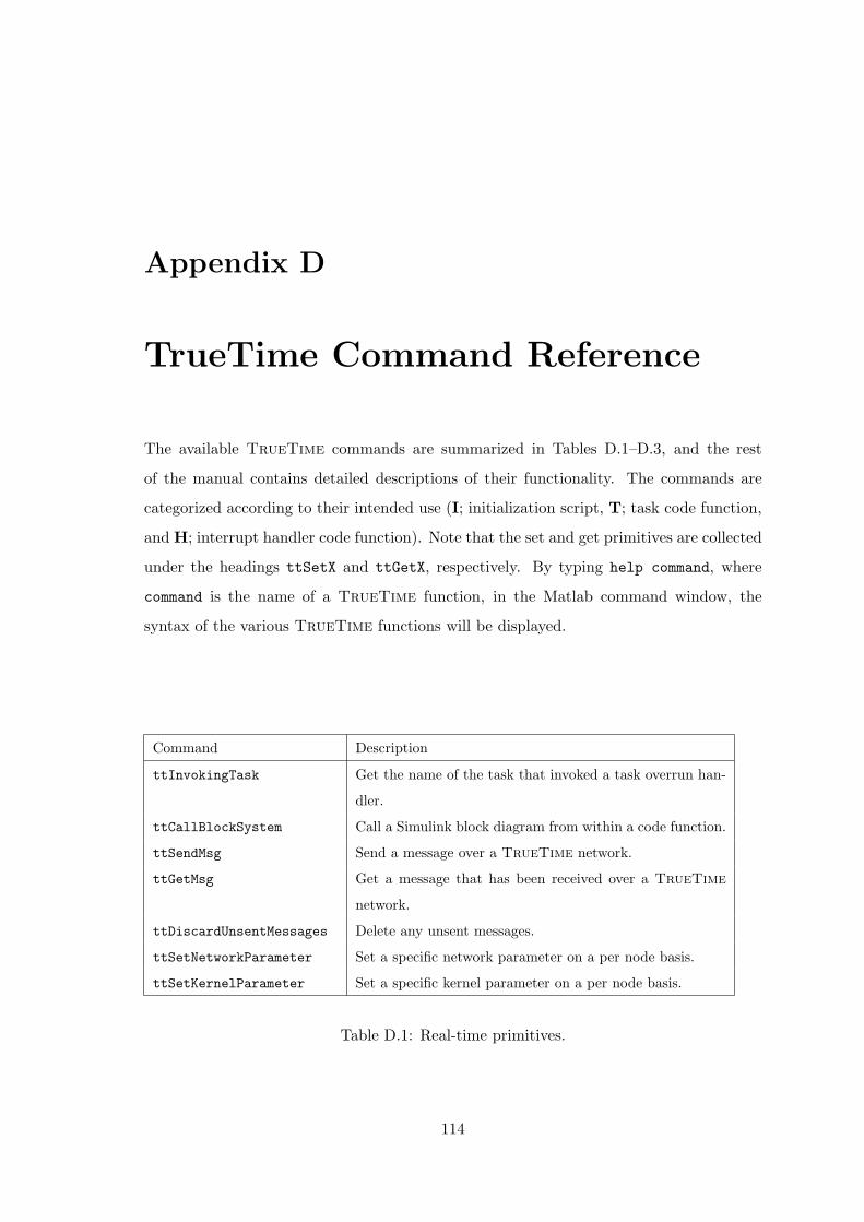
C.5. Packets loss and prediction
ing which new data aren’t received by the controller), using an output predictor, the
performance of the loop can be improved.
113
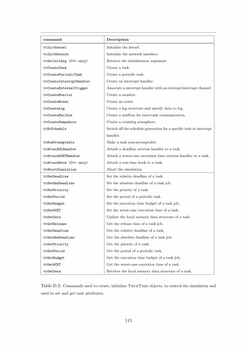
Appendix D
TrueTime Command Reference
The available TrueTime commands are summarized in Tables D.1–D.3, and the rest
of the manual contains detailed descriptions of their functionality. The commands are
categorized according to their intended use (I; initialization script, T; task code function,
and H; interrupt handler code function). Note that the set and get primitives are collected
under the headings ttSetX and ttGetX, respectively. By typing help command, where
command is the name of a TrueTime function, in the Matlab command window, the
syntax of the various TrueTime functions will be displayed.
Command Description
ttInvokingTask Get the name of the task that invoked a task overrun han-
dler.
ttCallBlockSystem Call a Simulink block diagram from within a code function.
ttSendMsg Send a message over a TrueTime network.
ttGetMsg Get a message that has been received over a TrueTime
network.
ttDiscardUnsentMessages Delete any unsent messages.
ttSetNetworkParameter Set a specific network parameter on a per node basis.
ttSetKernelParameter Set a specific kernel parameter on a per node basis.
Table D.1: Real-time primitives.
114
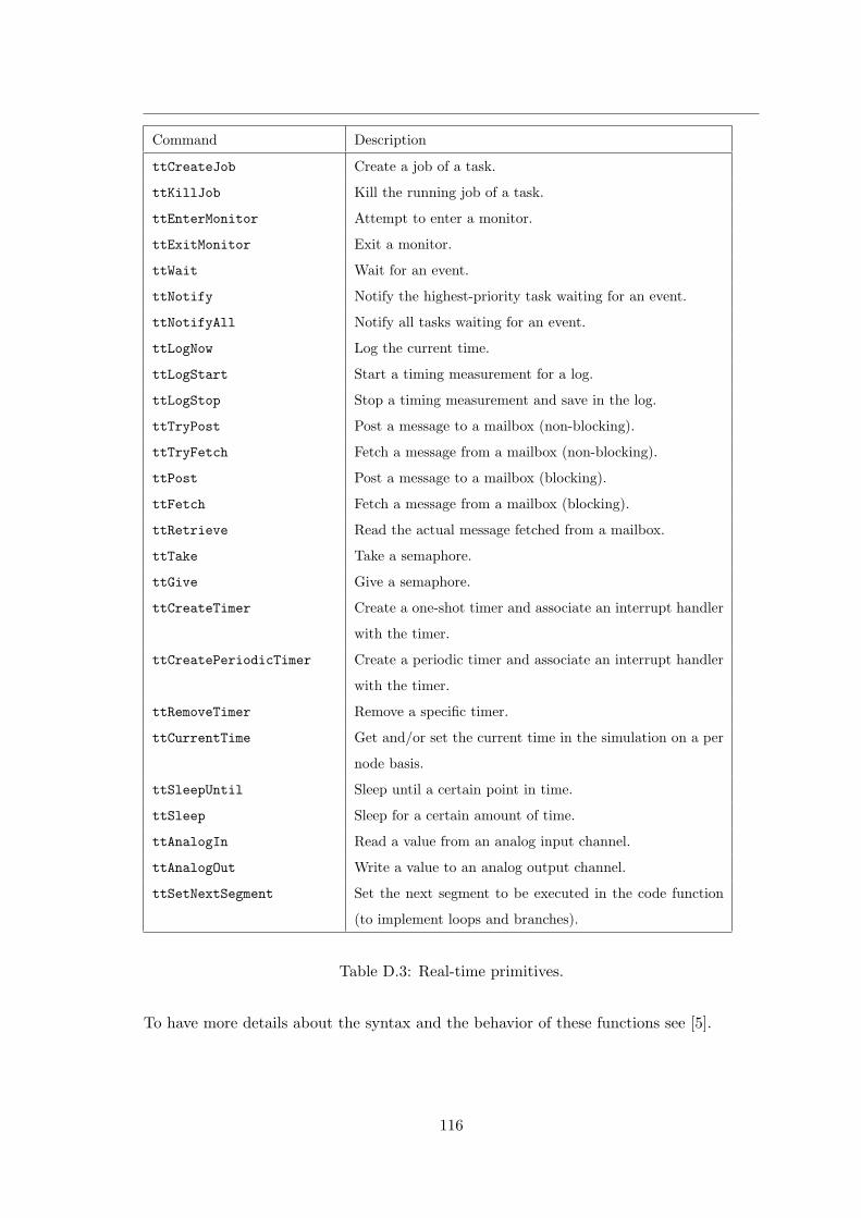
command Description
ttInitKernel Initialize the kernel.
ttInitNetwork Initialize the network interface.
ttGetInitArg (C++ only) Retrieve the initialization argument.
ttCreateTask Create a task.
ttCreatePeriodicTask Create a periodic task.
ttCreateInterruptHandler Create an interrupt handler.
ttCreateExternalTrigger Associate a interrupt handler with an external interrupt channel.
ttCreateMonitor Create a monitor.
ttCreateEvent Create an event.
ttCreateLog Create a log structure and specify data to log.
ttCreateMailbox Create a mailbox for inter-task communication.
ttCreateSempahore Create a counting semaphore.
ttNoSchedule Switch off the schedule generation for a specific task or interrupt
handler.
ttNonPreemptable Make a task non-preemptable.
ttAttachDLHandler Attach a deadline overrun handler to a task.
ttAttachWCETHandler Attach a worst-case execution time overrun handler to a task.
ttAttachHook (C++ only) Attach a run-time hook to a task.
ttAbortSimulation Abort the simulation.
ttSetDeadline Set the relative deadline of a task.
ttSetAbsDeadline Set the absolute deadline of a task job.
ttSetPriority Set the priority of a task.
ttSetPeriod Set the period of a periodic task.
ttSetBudget Set the execution time budget of a task job.
ttSetWCET Set the worst-case execution time of a task.
ttSetData Update the local memory data structure of a task.
ttGetRelease Get the release time of a task job.
ttGetDeadline Get the relative deadline of a task.
ttGetAbsDeadline Get the absolute deadline of a task job.
ttGetPriority Get the priority of a task.
ttGetPeriod Get the period of a periodic task.
ttGetBudget Get the execution time budget of a task job.
ttGetWCET Get the worst-case execution time of a task.
ttGetData Retrieve the local memory data structure of a task.
Table D.2: Commands used to create, initialize TrueTime objects, to control the simulation and
used to set and get task attributes.
115
Command Description
ttCreateJob Create a job of a task.
ttKillJob Kill the running job of a task.
ttEnterMonitor Attempt to enter a monitor.
ttExitMonitor Exit a monitor.
ttWait Wait for an event.
ttNotify Notify the highest-priority task waiting for an event.
ttNotifyAll Notify all tasks waiting for an event.
ttLogNow Log the current time.
ttLogStart Start a timing measurement for a log.
ttLogStop Stop a timing measurement and save in the log.
ttTryPost Post a message to a mailbox (non-blocking).
ttTryFetch Fetch a message from a mailbox (non-blocking).
ttPost Post a message to a mailbox (blocking).
ttFetch Fetch a message from a mailbox (blocking).
ttRetrieve Read the actual message fetched from a mailbox.
ttTake Take a semaphore.
ttGive Give a semaphore.
ttCreateTimer Create a one-shot timer and associate an interrupt handler
with the timer.
ttCreatePeriodicTimer Create a periodic timer and associate an interrupt handler
with the timer.
ttRemoveTimer Remove a specific timer.
ttCurrentTime Get and/or set the current time in the simulation on a per
node basis.
ttSleepUntil Sleep until a certain point in time.
ttSleep Sleep for a certain amount of time.
ttAnalogIn Read a value from an analog input channel.
ttAnalogOut Write a value to an analog output channel.
ttSetNextSegment Set the next segment to be executed in the code function
(to implement loops and branches).
Table D.3: Real-time primitives.
To have more details about the syntax and the behavior of these functions see [5].
116
Bibliography
[1] HART communication foundation - TDMA Data Link Layer - HCF SPEC − 075
Revision 1.0, 2007.
[2] HART communication foundation - Wireless Devices Specification - HCF SPEC −290 Revision 1.0, 2007.
[3] HART communication foundation - Network Management Specification -
HCF SPEC − 085, Revision 1.0, 2007.
[4] J. Song, S. Han, A, K, Mok, D. Chen, M. Lucas, M. Nixon, W. Pratt - WirelessHART:
Applying Wireless Technology in Real-Time Industrial Process Control - 14th IEEE
Real-Time and Embedded Technology and Applications Symposium (RTAS), 2007
[5] M. Ohlin, D. Henriksson, A. Cervin - TRUETIME 1.5-Reference Manual - Depart-
ment of Automatic Control Lund University, 2007.
[6] J. Song, A. K. Mork, D. Chen, Mark Nixon, T. Blevins, W. Wojsznis - Improving
PID Control with Unreliable Communications - ISA EXPO 2006, 17-19 October 2006
[7] D. Chen, M. Nixon, T. Aneweer, A. K. Mok, R. Shepard, T. Blevins, Greg McMillan
- Similarity-Based Traffic Reduction to Increase Battery Life in a Wireless Process
Control Network - ISA EXPO 2005, 2005
[8] K. J.Astrom, Tore Hagglund: PID control - Theory, Design, and Tuning- ISA, 1995
[9] K. J. Astrom, T. Hagglund, Advanced PID control - ISA, 2006
[10] J.P. Hespanha , P. Naghshtabrizi , Xu Yonggang -A Survey of Recent Results in
Networked Control Systems - Proceedings of the IEEE, Volume: 95, pages: 138-162,
2007
117
BIBLIOGRAPHY
[11] J. Nilsson, B. Bernhardsson, B. Wittenmark, Department of Automatic Control, Lund
Institute of Technology -Stochastic Analysis and Control of Real-Time Systems with
Random Time Delays - Automatica (Journal of IFAC) archive, Volume 34, pages:
57-64, 1998
[12] A. Ingimundarson , T. Hagglund - Performance comparison between PID and dead-
time compensating controllers - Journal of Process Control, Volume 12, Number 8,
pages: 887-895(9), 2002
[13] T. Keller J. Modelski - Experimental results of testing interferences in 2.4 GHz ISM
band - In Proc. 33rd European Microwave Conference, Munich, pages 1043-1046, 2003
[14] J.-A. Park, S.-K. Park, D.-H. Kim, P.-D. Cho and K.-R. Cho - Experiments on radio
interference between wireless lan and other radio devices on a 2.4 GHz ISM band -
57th IEEE Semiannual Vehicular Technology Conference. VTC 2003, Volume 3, pages
1798-1801, 2003
[15] M.V.S. Chandrashekhar, P. Choi, K. Maver, R. Sieber and K.Pahlavan - Evaluation
of interference between IEEE 802.11b and bluetooth in a typical office environment
- Proceedings 12th IEEE International Symposium on Personal, Indoor and Mobile
Radio Communications. PIMRC 2001, Volume 1, pages D71-D75, 2001
[16] V. E. Makensen and W. Kuntz - Bluetooth ZigBee and nanoNE Comparison of short-
range wireless personal area networks - Elektronik/Automotive, Volume 54, part 24,
pages 70-77
[17] A. C. Davies - An overview of Bluetooth Wireless TechnologyTMand some competing
LAN Standards - ICCSC 02, pages 206-211, 2002
[18] N. Abeamson -The ALOHA system - Another alternative for computer communica-
tions - AFIPS Conference Proceedings, Vol. 36, pages 295-298, 1970.
[19] A. S. Tanenbaum - Computer Networks - Fourth Edition, 2003
[20] A. Willig, K. Matheus, A. Wolisz - Wireless Technology in Industrial Networks -
Proceedings of the IEEE, Vol. 93, pages 1130-1151, 2005
[21] G. Olsson, C. Rosen - Industrial Automation - Lund Universtity, 2004
118

BIBLIOGRAPHY
[22] SOCRADES documents - Service-Oriented Cross-layer infRAstructure for Distributed
smart Embedded devices - www.socrades.eu
[23] S. Mangold, S. Choi, N. Esseling - An Error for Radio Transmitting Of Wireless
LANs at 5GHz - Proc. 10th Aachen Symposium on Signal Theory, pages 209-214,
2001
[24] IndustrialIT 800xA - System ( version 5.0) - System guide: Technical data and con-
figuration information- ABB Automation Technology Products
[25] IndustrialIT 800xA - Control and I/O ( System version 5.0) - Application programming
introduction and design- ABB Automation Technology Products
[26] R. Tjoa, K.L Chee, P. K. Sivaprasad, S.V. Rao and J.G. Lim - Clock Drift Reduction
for Relative Time Slot TDMA-based Sensor Networks - PIMRC 2004, 15-th IEEE
symposium, Volume 2, pages 1042-1047, 2004.
[27] http://www.ZigBee.org
[28] J. R. Moyne, D. M. Tilbury - The Emergence of Industrial Control Networks for Man-
ufacturing Control, Diagnostic, and Safety Data - Proceedings of the IEEE, Volume:
95, pages: 29-47, 2007
119