Embed Size (px)
Citation preview
Design of an Image-based FuzzyController for Parking Problems of a
Car-like Mobile Robot
YIN YIN AYE
Department of Intelligent Mechanical SystemsOkayama University
This dissertation is submitted for the degree ofDoctor of Philosophy in Engineering
March 2017


Acknowledgements
The success of research work in this thesis became possible due to a lot of help from manypeople during my Ph.D. study at Okayama University.
Firstly, I would like to express my deepest gratitude to my advisor, Professor KeigoWatanabe, for his valuable guidance, encouragement, patience, motivation and support incompleting the research work in this thesis. His teaching and guidelines have served as a rolemodel for me not only in academic but also in personal life.
I wish to express my thanks to Associate Professor Shoichi Maeyama and AssistantProfessor Isaku Nagai for their suggestions and comments throughout my Ph.D. reserach.Their kind guidance, encouragement, and patience have been great support throughout myresearch.
I would like to thank my thesis committee members, Professor Mamoru Minami andProfessor Akio Gofuku, for their encouragement, insightful comments and reviewing thisdissertation. I feel proud and honoured that you have accepted to be on my committee.
My sincere thanks also go to all my friends and colleagues at our laboratory for thepleasant atmosphere. Everyone has been open-minded to discussions which were contributedto this dissertation. This thesis could not have been done without the help and support ofnumerous people. Especially, I would like to thank Dr. Kimiko Motonaka and Mr. MaierdanMaimaitimin for their fruitful discussions and invaluable assistant they provided me in allphases of my work, especially in image-based fuzzy control and optimization of fuzzycontroller using a genetic algorithm.
I am deeply grateful to Mr. Junya Ukida , Mr. Hikaru Fujioka, and Mr. Toshiyuki Kageyufor their providing deep insights and cooperation on the development of image-based fuzzycontrol and for their technical support in the experiments.
Due to the support from people around me, I survived in Japan, in both academicand personal life. I also would like to thank all previous and current student members ofMechatronic Systems Laboratory, who have been very helpful not only in laboratory butalso in personal matters. I also would like to thanks the staff from Department of IntelligentMechanical Systems and Centre of Global Partnerships and Education for their kind helpduring my stay in Okayama University.
iv
The writing of this dissertation became possible due to the financial support by JapanInternational Cooperation Agency (JICA), Mechatronic Systems Laboratory and OkayamaUniversity.
Finally, I would like to offer my special thanks to my parents, brother and sister, whoalways give encouragement, support and good advices.
Abstract
With increasing number of vehicles over years, parking systems have become an importantissue in commercial environments such as shopping malls and airports. For this reason, theautomatic parking systems of car-like mobile robots have attracted a great deal of attentionfrom research organization and automobile industry. In many recent works, a number ofdifferent approaches have been developed to build an automatic parking system. Most ofthem are still expensive for commercialization.
In the middle of 80-th, the first ideas of automatic parking systems were developed.Under this topic, a fuzzy algorithm for garage parking system, a first nonlinear algorithm forparking control, and the main statements for parallel parking problem, were proposed as earlyresearches. Most of the researches related to a parking problem are usually to find a path thatconnects the initial configuration to the final one by considering the nonholonomic constraints.On the other hand, a skill-based approach that used the fuzzy logic, was developed. Thereis no reference path to be followed by a robot and the control command is generated byconsidering the position and orientation of the robot relative to the parking space. An exactvehicle pose relative to the parking space is required in this approach. The automatic parkingsystem consists of a parking lot detection module and an automatic parking algorithm. In therecent works on parking control systems, a method for detecting camera vision-based parkinglots and a method which used the ultrasonic sensors to detect the parking lots, were discussed.For the experimental study of fuzzy garage parking control, the CCD camera was utilized todetect the overall vision of the parking lot, the six infrared sensors were adopted to measurethe distances between the robot and the surroundings, and the sensor fusion techniques thatcombine the ultrasonic sensors, encoders, and gyroscopes with a differential GPS systemwere used to detect and estimate the dimensions of the parking lot in recent works. However,all are the expensive methods.
This thesis aims to build an automatic parking system of a car-like mobile robot. Theautomatic parking system that corresponds to the posture stabilization problem of car-likemobile robot, is presented in the first part of this dissertation. The goal is to stabilize thecar-like mobile robot to a desired final posture starting from any initial posture (posturemeans the combination of the position and orientation of the robot). The switching and
vi
non-switching controllers have been developed for stabilizing the car-like mobile robot thatwas a nonholonomic underactuated system with two inputs and four outputs. Since thissystem cannot be stabilized by a static continuous feedback with constant gains, there areseveral control methods by using a canonical form up to now such as chained form, a powerform, a Goursat normal form and a double integrator model. In the first part of this thesis,after obtaining a chained form, the invariant manifold technique was applied for stabilizingthe car-like mobile robot in the desired posture. The performances of the proposed controllersfor parking problem were verified through some computer simulations.
An image-based fuzzy controller for autonomous parking of a car-like mobile robotis presented in the second part of this thesis. In recent past, vision sensor and digitalimage processing technology become easily available with the development of computertechnology. Moreover, a vision sensor can be used to measure the environment withoutphysical contact. Visual servoing, which control the motion of the robot using one or morecameras, are conventionally classified in four groups: position-based visual servoing (PBVS),image-based visual servoing (IBVS), hybrid visual servoing (HVS), and motion-based visualservoing (MBVS). The aim of the second part of this thesis is to build a parking controllerupon the concepts of IBVS. In the IBVS, both of the control objective and the control lawdesign are directly performed in the image feature parameter space and thus the full model ofthe object need not be known accurately. To combine the behavior of the robot with the imagefeatures, a model-free fuzzy controller was designed without estimating the image depthin this work. The second part of thesis presents an automatic parking system of a car-likemobile robot using image-based fuzzy control. The proposed system receives the imageinformation about the parking frame from a web camera which is equipped on the top of therobot, and then generates the desired target line to be followed by the robot using Houghtransform. A fuzzy controller is designed with a reasoning mechanism composed of twoinputs, which are the slope and intercept of the target line, and one output that is the steeringangle of the robot. The results of both simulation and real robot experiments confirmed thatour image-based fuzzy controller is effective and feasible for parking problem.
In the third part of this thesis, a genetic algorithm (GA) was used to optimize theparameters of membership functions of an image-based fuzzy parking controller. It is wellknown that the process of manually tuning a fuzzy logic controller is a very complex task,which consists of choosing the type of fuzzy logic controller, the number and shape ofmembership functions of inputs and outputs, and the rule base. The image-based fuzzycontroller for parking problem of the car-like mobile robot was developed in the secondpart of this thesis, where the membership functions and fuzzy rules were tuned manuallyby trial and error. The aim of the last part of this thesis is to optimize the parameters of the
vii
membership functions by using the GA against the complicated tuning of the controller. Thefuzzy rules are constructed based on the skills of the experienced human drivers in advanceand the GA was not used to optimize the rules set of the fuzzy controller. Simulation resultsare given to demonstrate the effectiveness of the optimized image-based fuzzy controller byGA.

Table of contents
List of figures xiii
List of tables xvii
1 Introduction 11.1 Motivation . . . . . . . . . . . . . . . . . . . . . . . . . . . . . . . . . . . 11.2 Aims of the Thesis . . . . . . . . . . . . . . . . . . . . . . . . . . . . . . 21.3 Major Contributions . . . . . . . . . . . . . . . . . . . . . . . . . . . . . . 21.4 Organization . . . . . . . . . . . . . . . . . . . . . . . . . . . . . . . . . . 31.5 Publications . . . . . . . . . . . . . . . . . . . . . . . . . . . . . . . . . . 4
2 Background Research 72.1 Stabilizing Control Using Invariant Manifolds . . . . . . . . . . . . . . . . 72.2 Visual Servoing . . . . . . . . . . . . . . . . . . . . . . . . . . . . . . . . 9
2.2.1 Position-based visual servoing (PBVS) . . . . . . . . . . . . . . . 102.2.2 Image-based visual servoing (IBVS) . . . . . . . . . . . . . . . . . 112.2.3 Hybrid visual servoing . . . . . . . . . . . . . . . . . . . . . . . . 132.2.4 Motion-based visual servoing . . . . . . . . . . . . . . . . . . . . 13
2.3 Mobile Robot Control Using Fuzzy Logic . . . . . . . . . . . . . . . . . . 142.4 Optimized Fuzzy Controller by Genetic Algorithms . . . . . . . . . . . . . 162.5 Summary . . . . . . . . . . . . . . . . . . . . . . . . . . . . . . . . . . . 18
3 Invariant Manifold-based Stabilizing Controllers for Parking Problems 193.1 Problem Setting . . . . . . . . . . . . . . . . . . . . . . . . . . . . . . . . 203.2 Derivation of Invariant Manifold . . . . . . . . . . . . . . . . . . . . . . . 233.3 Attractive Control to the Manifold . . . . . . . . . . . . . . . . . . . . . . 25
3.3.1 Switching controller I . . . . . . . . . . . . . . . . . . . . . . . . 253.3.2 Switching controller II . . . . . . . . . . . . . . . . . . . . . . . . 263.3.3 Switching controller III . . . . . . . . . . . . . . . . . . . . . . . . 26
x Table of contents
3.3.4 Non-switching controller . . . . . . . . . . . . . . . . . . . . . . . 273.4 Simulation Experiments . . . . . . . . . . . . . . . . . . . . . . . . . . . . 293.5 Summary . . . . . . . . . . . . . . . . . . . . . . . . . . . . . . . . . . . 33
4 Image-based Fuzzy Parking Control of a Car-like Mobile Robot 394.1 Problem Setting . . . . . . . . . . . . . . . . . . . . . . . . . . . . . . . . 404.2 Generation of the Target Line Based on Image Processing . . . . . . . . . . 43
4.2.1 Thresholding of the parking space . . . . . . . . . . . . . . . . . . 434.2.2 Extraction of the parking lines using Hough transformation . . . . . 43
4.3 Fuzzy Parking Control . . . . . . . . . . . . . . . . . . . . . . . . . . . . 464.3.1 Fuzzification of state variables . . . . . . . . . . . . . . . . . . . . 474.3.2 Calculation of grade of each rule . . . . . . . . . . . . . . . . . . . 484.3.3 Defuzzification of input values . . . . . . . . . . . . . . . . . . . . 49
4.4 Experiments . . . . . . . . . . . . . . . . . . . . . . . . . . . . . . . . . . 524.4.1 Simulation experiments . . . . . . . . . . . . . . . . . . . . . . . 524.4.2 Real robot experiments . . . . . . . . . . . . . . . . . . . . . . . . 55
4.5 Summary . . . . . . . . . . . . . . . . . . . . . . . . . . . . . . . . . . . 57
5 Optimization of an Image-based Fuzzy Controller by a Genetic Algorithm 655.1 Problem Setting . . . . . . . . . . . . . . . . . . . . . . . . . . . . . . . . 655.2 Image-based Fuzzy Parking Controller . . . . . . . . . . . . . . . . . . . . 685.3 Optimization of Membership Functions by GA . . . . . . . . . . . . . . . 70
5.3.1 Chromosome and initialization . . . . . . . . . . . . . . . . . . . . 715.3.2 Evaluation function . . . . . . . . . . . . . . . . . . . . . . . . . . 725.3.3 GA operators . . . . . . . . . . . . . . . . . . . . . . . . . . . . . 73
5.4 Simulation Experiment . . . . . . . . . . . . . . . . . . . . . . . . . . . . 735.5 Summary . . . . . . . . . . . . . . . . . . . . . . . . . . . . . . . . . . . 76
6 Conclusion and Future Work 796.1 Concluding Remarks . . . . . . . . . . . . . . . . . . . . . . . . . . . . . 796.2 Future Work . . . . . . . . . . . . . . . . . . . . . . . . . . . . . . . . . . 80
References 81
Appendix A Mamdani Fuzzy Inference System 91
Appendix B Sugeno Fuzzy Inference System 93

Table of contents xi
Appendix C Genetic Algorithms 95

List of figures
2.1 Wheeled mobile robots: (a) Pinoneer 3-AT, (b) 4WD aluminum, (c) 3WD100 mm omni wheel mini, and (d) Ris-RSummit . . . . . . . . . . . . . . . 9
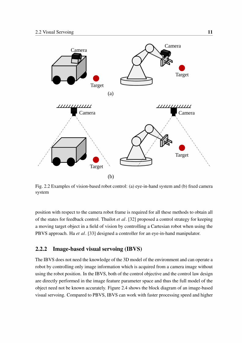
2.2 Examples of vision-based robot control: (a) eye-in-hand system and (b) fixedcamera system . . . . . . . . . . . . . . . . . . . . . . . . . . . . . . . . . 11
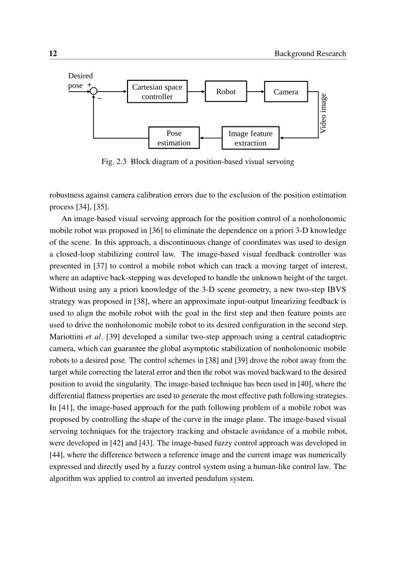
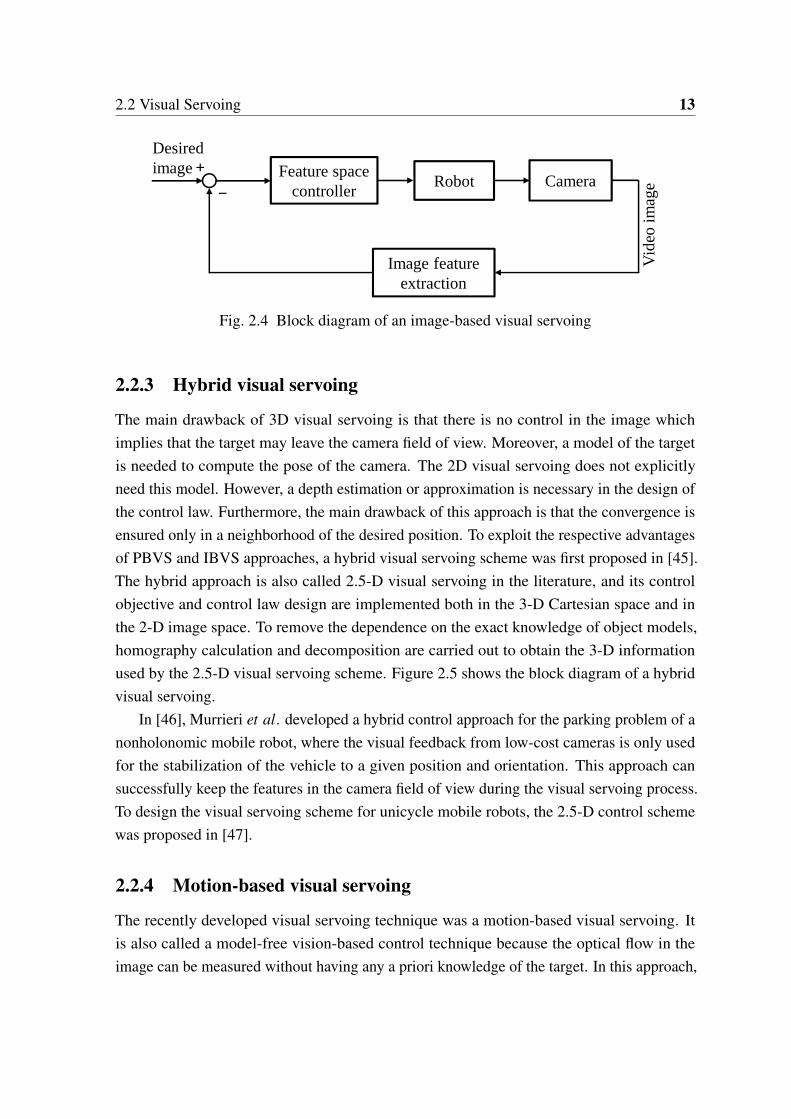
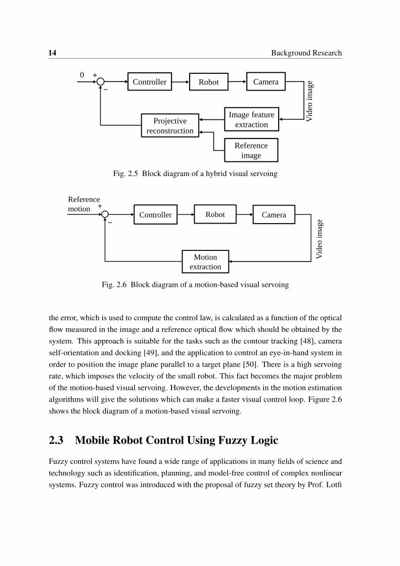
2.3 Block diagram of a position-based visual servoing . . . . . . . . . . . . . . 122.4 Block diagram of an image-based visual servoing . . . . . . . . . . . . . . 132.5 Block diagram of a hybrid visual servoing . . . . . . . . . . . . . . . . . . 142.6 Block diagram of a motion-based visual servoing . . . . . . . . . . . . . . 142.7 Basic fuzzy mobile robot control loop . . . . . . . . . . . . . . . . . . . . 152.8 Genetic algorithm flowchart . . . . . . . . . . . . . . . . . . . . . . . . . 17
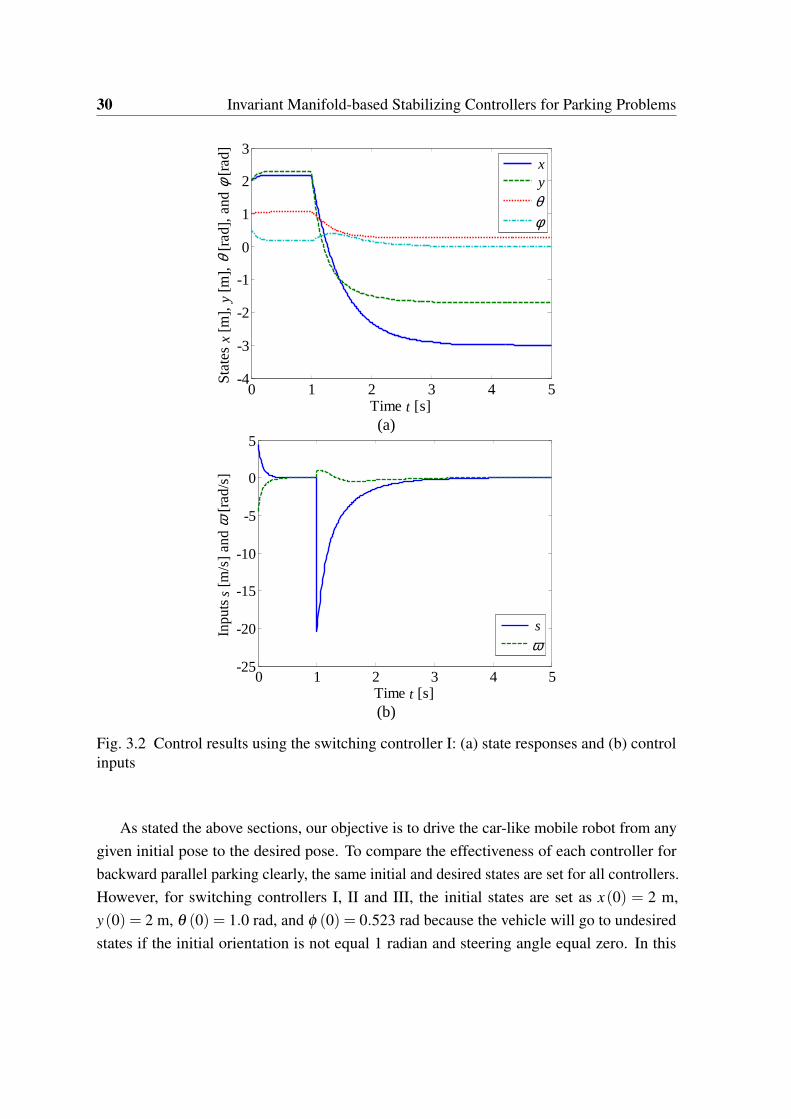
3.1 Configuration of a car-like mobile robot . . . . . . . . . . . . . . . . . . . 203.2 Control results using the switching controller I: (a) state responses and (b)
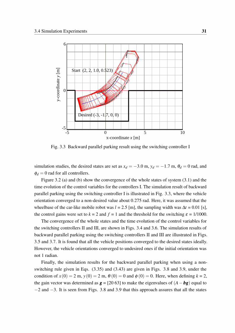
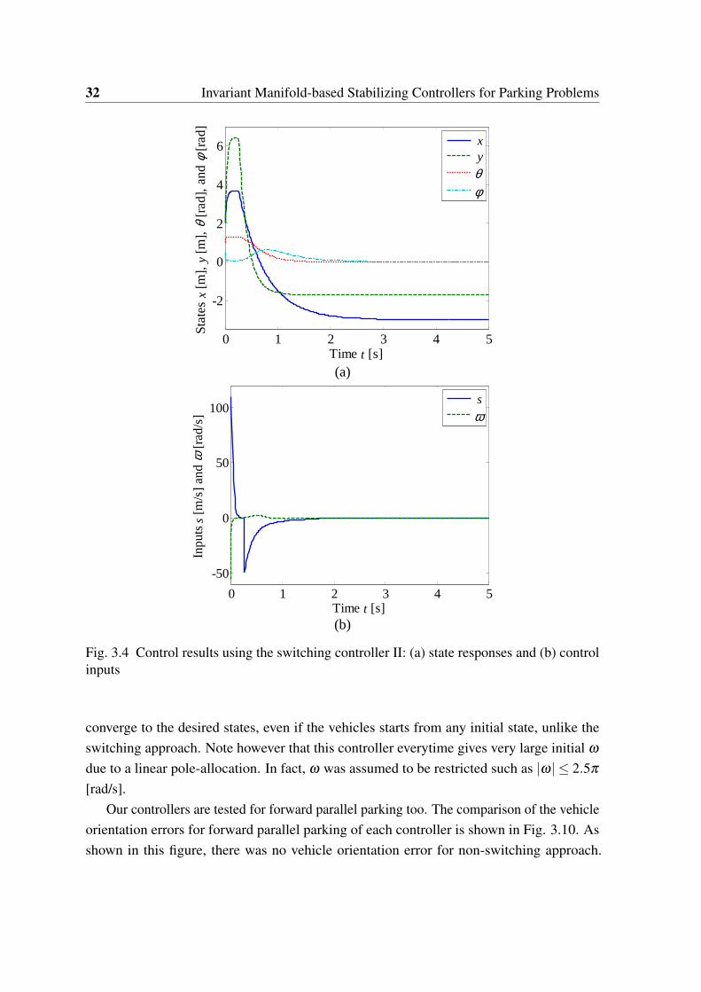
control inputs . . . . . . . . . . . . . . . . . . . . . . . . . . . . . . . . . 303.3 Backward parallel parking result using the switching controller I . . . . . . 313.4 Control results using the switching controller II: (a) state responses and (b)
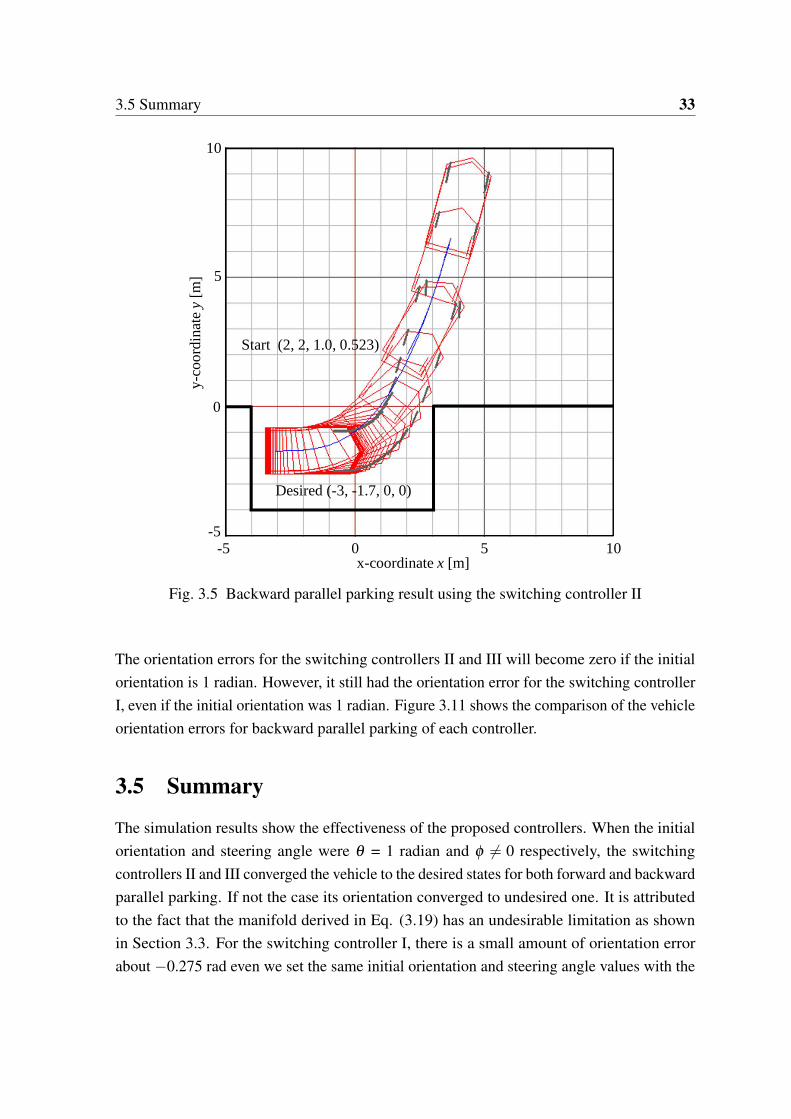
control inputs . . . . . . . . . . . . . . . . . . . . . . . . . . . . . . . . . 323.5 Backward parallel parking result using the switching controller II . . . . . . 333.6 Control results using the switching controller III: (a) state responses and (b)
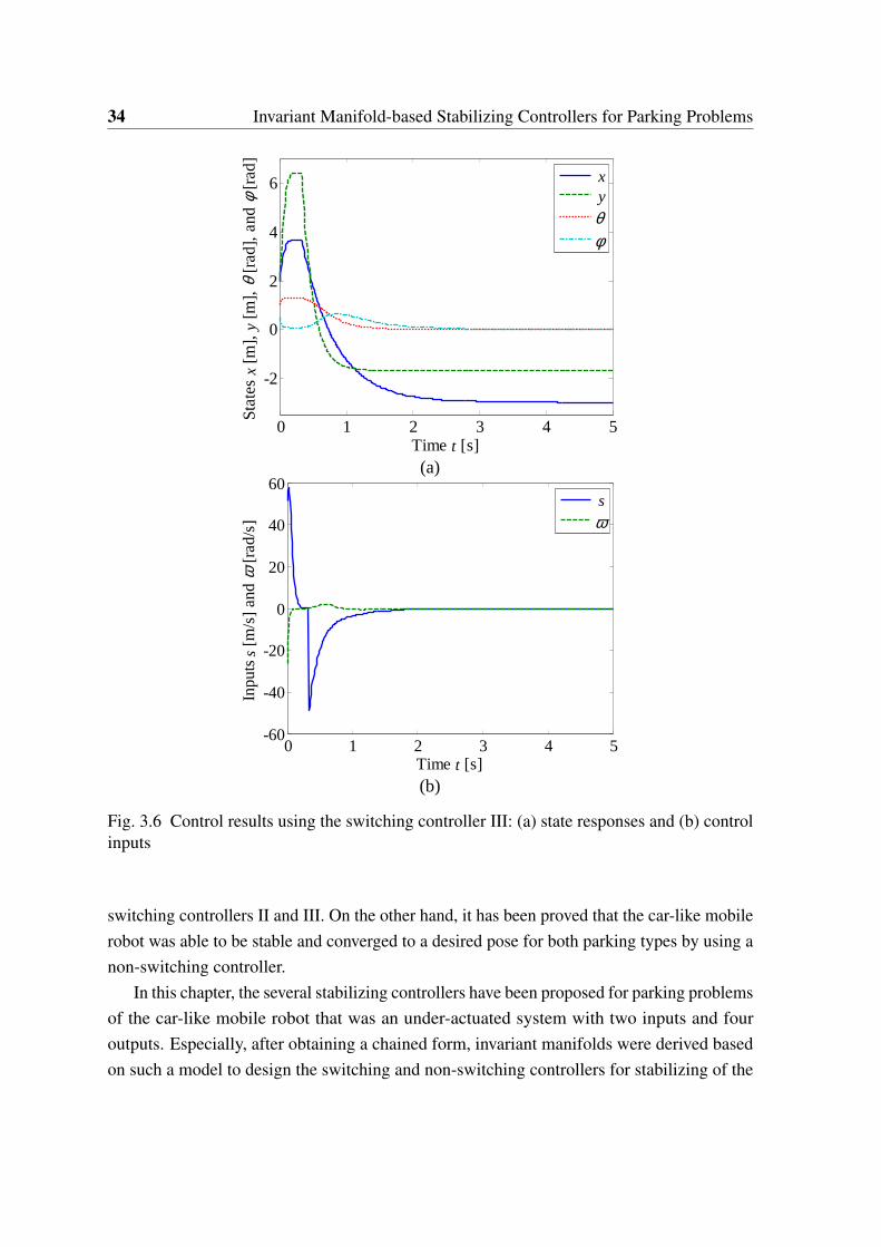
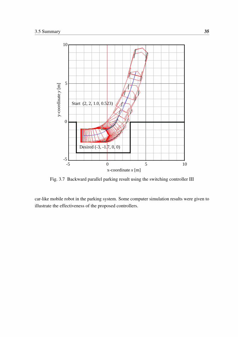
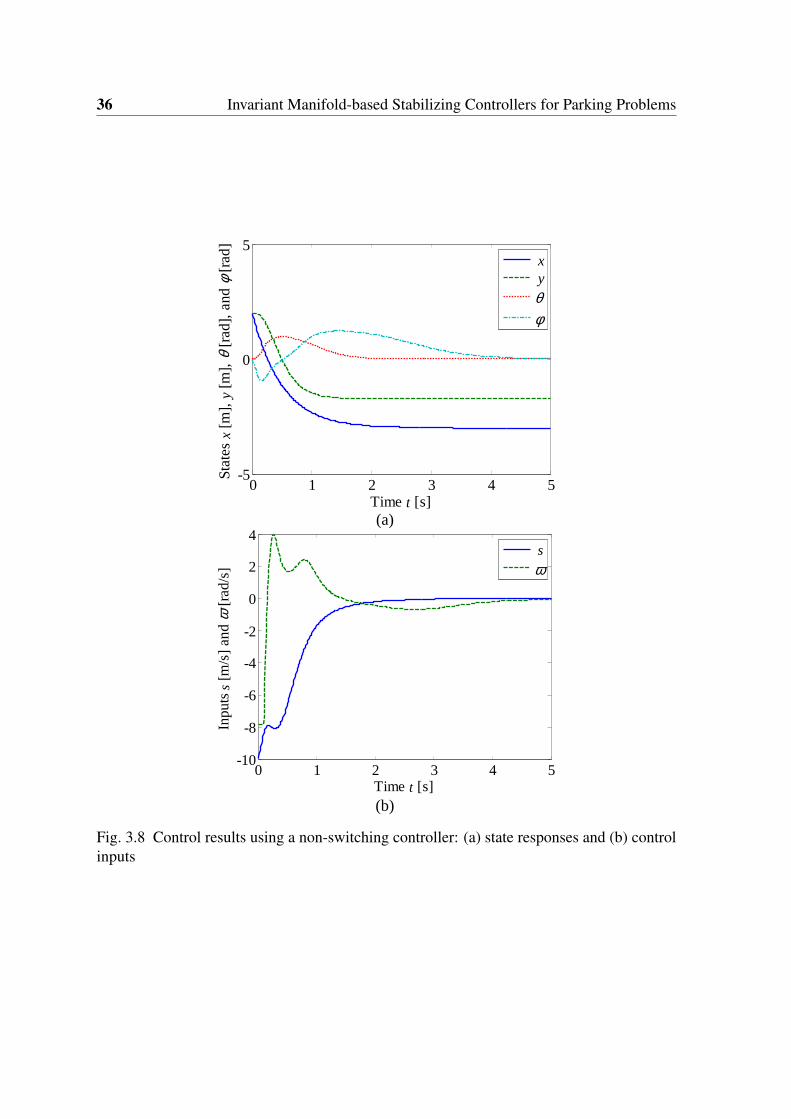
control inputs . . . . . . . . . . . . . . . . . . . . . . . . . . . . . . . . . 343.7 Backward parallel parking result using the switching controller III . . . . . 353.8 Control results using a non-switching controller: (a) state responses and (b)
control inputs . . . . . . . . . . . . . . . . . . . . . . . . . . . . . . . . . 363.9 Backward parallel parking result using a non-switching controller . . . . . 373.10 Comparison of vehicle orientation errors for forward parallel parking . . . 373.11 Comparison of vehicle orientation errors for backward parallel parking . . 38
4.1 Experimental overview . . . . . . . . . . . . . . . . . . . . . . . . . . . . 40
xiv List of figures
4.2 Coordinate systems used for the automatic parking system: (a) world coordi-nate and (b) image coordinate . . . . . . . . . . . . . . . . . . . . . . . . . 41
4.3 Block diagram of the image-based fuzzy parking control . . . . . . . . . . 424.4 Image processing algorithm . . . . . . . . . . . . . . . . . . . . . . . . . . 434.5 Image of the parking frame: (a) the original image and (b) the preprocessed
image . . . . . . . . . . . . . . . . . . . . . . . . . . . . . . . . . . . . . 444.6 Canny edge detection: (a) binary image and (b) result image after hough
transform . . . . . . . . . . . . . . . . . . . . . . . . . . . . . . . . . . . 444.7 Center line of the parking frame: (a) result image after grouping and (b)
result of the center line . . . . . . . . . . . . . . . . . . . . . . . . . . . . 454.8 Line representations: (a) when using parameters ρ and δ and (b) when using
the starting and ending points ((u0,v0) and (u1,v1)) of a line on the image plane 454.9 Desired target line started from (a) left side and (b) right side, of the parking
frame . . . . . . . . . . . . . . . . . . . . . . . . . . . . . . . . . . . . . 464.10 Structure of the image-based fuzzy controller . . . . . . . . . . . . . . . . 464.11 Membership functions: (a) for the input variables αt and βt , and (b) for the
output variable φ . . . . . . . . . . . . . . . . . . . . . . . . . . . . . . . 484.12 Min-max algorithm . . . . . . . . . . . . . . . . . . . . . . . . . . . . . . 504.13 Notations for the angle and perpendicular parking . . . . . . . . . . . . . . 514.14 History of parameters related to angle parking . . . . . . . . . . . . . . . . 514.15 Simulation result of angle parking . . . . . . . . . . . . . . . . . . . . . . 524.16 History of parameters related to perpendicular parking, case 1 . . . . . . . 534.17 Simulation result of perpendicular parking, case 1 . . . . . . . . . . . . . . 534.18 History of parameters related to perpendicular parking, case 2 . . . . . . . 544.19 Simulation result of perpendicular parking, case 2 . . . . . . . . . . . . . . 554.20 Membership functions: (a) for the input variables αt and βt , and (b) for the
output variable φ for the 25 fuzzy rules . . . . . . . . . . . . . . . . . . . . 574.21 History of the parameters related to perpendicular parking (case 1), when
used the 25 fuzzy rules . . . . . . . . . . . . . . . . . . . . . . . . . . . . 584.22 Simulation result of perpendicular parking (case 1), when used the 25 fuzzy
rules . . . . . . . . . . . . . . . . . . . . . . . . . . . . . . . . . . . . . . 594.23 Experimental robot . . . . . . . . . . . . . . . . . . . . . . . . . . . . . . 594.24 Experimental results that used the 52 degree AOV camera, when started with
initial conditions (x, y, θ ) = (0.49 [m], 0.54 [m], −135 [deg]) . . . . . . . . 604.25 Experimental results that used the 52 degree AOV camera, when started with
initial conditions (x, y, θ ) = (−0.49 [m], 0.54 [m], −45 [deg]) . . . . . . . 61
List of figures xv
4.26 Experimental results of case 1, where the 120 degree AOV camera was used 624.27 Experimental results of case 2, where the 120 degree AOV camera was used 63
5.1 Overview of the environment and the definition of the coordinate . . . . . . 665.2 Controlled object . . . . . . . . . . . . . . . . . . . . . . . . . . . . . . . 665.3 Block diagram of an image-based fuzzy parking control method . . . . . . 675.4 Membership functions . . . . . . . . . . . . . . . . . . . . . . . . . . . . 695.5 Process to determine the control inputs, s and φ . . . . . . . . . . . . . . . 695.6 Chromosome-encoded membership function parameters and consequent . . 725.7 Score of the best individual . . . . . . . . . . . . . . . . . . . . . . . . . . 735.8 The desired target trajectory for perpendicular parking system . . . . . . . 745.9 Optimized trajectory path, when started with initial conditions (x, y, θ ) = (0,
−1, 0◦) . . . . . . . . . . . . . . . . . . . . . . . . . . . . . . . . . . . . 755.10 Simulation result after optimization process . . . . . . . . . . . . . . . . . 75
B.1 The Sugeno fuzzy model . . . . . . . . . . . . . . . . . . . . . . . . . . . 94
C.1 Illustration of parental crossover in genetic reproduction . . . . . . . . . . 96C.2 Illustration of mutation of a chromosome on the fifth gene . . . . . . . . . 97

List of tables
4.1 Fuzzy rules for the steering angle, φ . . . . . . . . . . . . . . . . . . . . . 494.2 Parameters of parking frame and initial postures of the vehicle . . . . . . . 514.3 Fuzzy rules for φ . . . . . . . . . . . . . . . . . . . . . . . . . . . . . . . 564.4 Specifications of the real robot experiments . . . . . . . . . . . . . . . . . 56
5.1 Important parameters of GA . . . . . . . . . . . . . . . . . . . . . . . . . 725.2 Optimized membership function parameters . . . . . . . . . . . . . . . . . 74

Chapter 1
Introduction
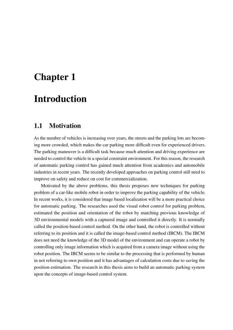
1.1 Motivation
As the number of vehicles is increasing over years, the streets and the parking lots are becom-ing more crowded, which makes the car parking more difficult even for experienced drivers.The parking maneuver is a difficult task because much attention and driving experience areneeded to control the vehicle in a special constraint environment. For this reason, the researchof automatic parking control has gained much attention from academics and automobileindustries in recent years. The recently developed approaches on parking control still need toimprove on safety and reduce on cost for commercialization.
Motivated by the above problems, this thesis proposes new techniques for parkingproblem of a car-like mobile robot in order to improve the parking capability of the vehicle.In recent works, it is considered that image based localization will be a more practical choicefor automatic parking. The researches used the visual robot control for parking problem,estimated the position and orientation of the robot by matching previous knowledge of3D environmental models with a captured image and controlled it directly. It is normallycalled the position-based control method. On the other hand, the robot is controlled withoutreferring to its position and it is called the image-based control method (IBCM). The IBCMdoes not need the knowledge of the 3D model of the environment and can operate a robot bycontrolling only image information which is acquired from a camera image without using therobot position. The IBCM seems to be similar to the processing that is performed by humanin not referring to own position and it has advantages of calculation costs due to saving theposition estimation. The research in this thesis aims to build an automatic parking systemupon the concepts of image-based control system.
2 Introduction
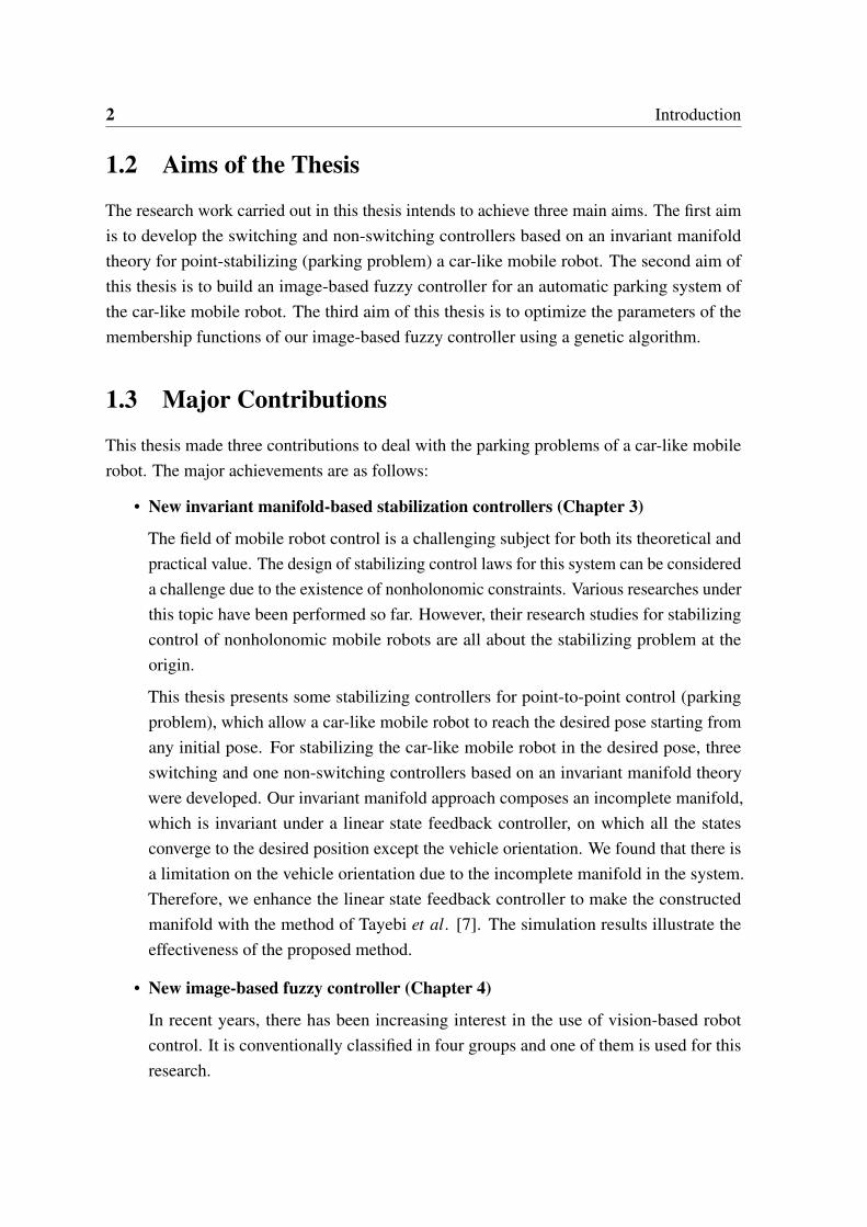
1.2 Aims of the Thesis
The research work carried out in this thesis intends to achieve three main aims. The first aimis to develop the switching and non-switching controllers based on an invariant manifoldtheory for point-stabilizing (parking problem) a car-like mobile robot. The second aim ofthis thesis is to build an image-based fuzzy controller for an automatic parking system ofthe car-like mobile robot. The third aim of this thesis is to optimize the parameters of themembership functions of our image-based fuzzy controller using a genetic algorithm.
1.3 Major Contributions
This thesis made three contributions to deal with the parking problems of a car-like mobilerobot. The major achievements are as follows:
• New invariant manifold-based stabilization controllers (Chapter 3)
The field of mobile robot control is a challenging subject for both its theoretical andpractical value. The design of stabilizing control laws for this system can be considereda challenge due to the existence of nonholonomic constraints. Various researches underthis topic have been performed so far. However, their research studies for stabilizingcontrol of nonholonomic mobile robots are all about the stabilizing problem at theorigin.
This thesis presents some stabilizing controllers for point-to-point control (parkingproblem), which allow a car-like mobile robot to reach the desired pose starting fromany initial pose. For stabilizing the car-like mobile robot in the desired pose, threeswitching and one non-switching controllers based on an invariant manifold theorywere developed. Our invariant manifold approach composes an incomplete manifold,which is invariant under a linear state feedback controller, on which all the statesconverge to the desired position except the vehicle orientation. We found that there isa limitation on the vehicle orientation due to the incomplete manifold in the system.Therefore, we enhance the linear state feedback controller to make the constructedmanifold with the method of Tayebi et al. [7]. The simulation results illustrate theeffectiveness of the proposed method.
• New image-based fuzzy controller (Chapter 4)
In recent years, there has been increasing interest in the use of vision-based robotcontrol. It is conventionally classified in four groups and one of them is used for thisresearch.
1.4 Organization 3
This thesis presents an automatic parking system of the car-like mobile robot usingan image-based fuzzy controller. To the best of our knowledge, there is no IBVScontroller developed for automatic parking system of car-like mobile robots. Theimage-based control method was able to reduce the amount of calculations becauseit did not need to perform the position estimation processes. The proposed systemenabled the car-like mobile robot to park towards the red color parking frame drawnon the floor. The results of simulation and real robot experiments are given to provethe effectiveness of the proposed control scheme.
• New optimized fuzzy controller by GA (Chapter 5)
In many recent works, the GA has been applied to optimize the fuzzy logic controllerand some self-tuning methods using GA have been proposed to reduce the requiredtuning efforts by human operators. To obtain a better performance of our image-basedfuzzy controller, it is very important to adjust the widths of membership functions ofinput and output variables.
This thesis presents an automatic parking system using an optimized image-based fuzzycontroller by a GA. It was proved that tuning of the shape of membership functions ofinput and output variables, can be automated by using the GA to optimize the proposedfuzzy controller in this thesis. The GA is not used to tune the fuzzy reasoning rules andthese are constructed based on the skills of the experienced human drivers in advance.In our research, genetic algorithm has introduced to reduce the required tuning effortsof the 81 fuzzy control rules by a human operator. The simulation results illustrate theeffectiveness of the developed schemes.
1.4 Organization
The chapter contents of this dissertation can be briefly summarized as follows:
Chapter 2 describes the background information that leads to conduct the research in thisthesis.
Chapter 3 proposes new switching and non-switching controllers based on an invariantmanifold theory for parking problems of a car-like mobile robot.
Chapter 4 devotes a novel method to design a car-like mobile robot that possesses au-tonomous angle parking and perpendicular parking capability by using an image-based fuzzycontroller.
Chapter 5 presents GA optimized image-based fuzzy controller for an automatic parking of
4 Introduction
a car-like mobile robot.
Chapter 6 concludes this thesis with a summary of the work carried out.
1.5 Publications
The research work presented in this thesis has resulted in the following publications.
Journals
1. Yin Yin Aye, Keigo Watanabe, Shoichi Maeyama, and Isaku Nagai, “Invariant manifold-based stabilizing controllers for nonholonomic mobile robots,” Artificial Life andRobotics, vol. 20, no. 3, pp. 276–284, 2015.
2. Yin Yin Aye, Keigo Watanabe, Shoichi Maeyama, and Isaku Nagai, “Image-basedfuzzy parking control of a car-like mobile robot,” International Journal on SmartMaterial and Mechatronics, vol. 3, no. 1, pp.160–164, 2016.
3. Yin Yin Aye, Keigo Watanabe, Shoichi Maeyama, and Isaku Nagai, “Design of animage-based fuzzy controller for autonomous parking of four-wheeled mobile robots,”International Journal of Applied Electromagnetics and Mechanics, vol. 52, no. 3-4,pp. 859–865, 2016.
4. Yin Yin Aye, Keigo Watanabe, Shoichi Maeyama, and Isaku Nagai, “An intelligentparking system for vehicles using an image-based fuzzy controller,” InternationalJournal on Smart Material and Mechatronics, (Accepted: 30, Dec. 2016).
5. Yin Yin Aye, Keigo Watanabe, Shoichi Maeyama, and Isaku Nagai, “An automaticparking system using an optimized image-based fuzzy controller by genetic algorithms,”Artificial Life and Robotics, vol. 22, no. 1, pp. 139–144, 2017.
International Conferences
1. Yin Yin Aye, Keigo Watanabe, Shoichi Maeyama, and Isaku Nagai, “Controllers basedon an invariant manifold approach for stabilizing a nonholonomic mobile robot,” inProceedings of the 7th International Conference on Soft Computing and IntelligentSystems and the 15th International Symposium on Advanced Intellligent Systems (SCIS& ISIS), pp. 134–139, Fukuoka, Japan, Dec. 2014.
2. Yin Yin Aye, Keigo Watanabe, Shoichi Maeyama, and Isaku Nagai, “Invariant manifold-based stabilizing controllers for nonholonomic mobile robot ,” in Proceedings of the
1.5 Publications 5
5th International Conference on Science and Engineering (ICSE), Yangon, Myanmar,Dec. 2014.
3. Yin Yin Aye, Keigo Watanabe, Shoichi Maeyama, and Isaku Nagai, “ Stabilization ofnonholonomic mobile robot using controllers based on an invariant manifold theory,”in Proceedings of the 20th International Symposium on Artificial Life and Robotics(AROB), pp. 537–542, Beppu, Japan, Jan. 2015.
4. Yin Yin Aye, Keigo Watanabe, Shoichi Maeyama, and Isaku Nagai, “Design of animage-based fuzzy controller for autonomous parking of four-wheeled mobile robots,”in Proceedings of the 17th International Symposium on Applied Electromagnetics andMechanics (ISEM), 2P1-D-1 isem2015-076.pdf, Kobe, Japan, Sept. 2015.
5. Yin Yin Aye, Keigo Watanabe, Shoichi Maeyama, and Isaku Nagai, “Automatic parkingof a car-like mobile robot using an image-based fuzzy controller,” in Proceedings ofthe 2nd International Conference on Smart Material and Mechatronics (ISSMM),pp. 62–66, Makassar, Indonesia, Oct. 2015.
6. Yin Yin Aye, Keigo Watanabe, Shoichi Maeyama, and Isaku Nagai, “Generation oftime-varying target lines for an automatic parking system using image-based process-ing,” in Proceedings of International Conference on Robotics and Biomimetics (IEEEROBIO), pp. 423–427, Zhuhai, China, Dec. 2015.
7. Yin Yin Aye, Keigo Watanabe, Shoichi Maeyama, and Isaku Nagai, “Optimizationof an image-based fuzzy controller for an automatic parking system using a geneticalgorithm,” in Proceedings of the 21th International Symposium on Artificial Life andRobotics (AROB), pp. 354–357, Beppu, Japan, Jan. 2016.
8. Yin Yin Aye, Keigo Watanabe, Shoichi Maeyama, and Isaku Nagai, “Image-basedfuzzy control of a car-like mobile robot for parking problems,” in Proceedings ofInternational Conference on Mechatronics and Automation (IEEE ICMA), pp. 502–507, Harbin, China, Aug. 2016.
9. Yin Yin Aye, Keigo Watanabe, Shoichi Maeyama, and Isaku Nagai, “An intelligentparking system for vehicles using an image-based fuzzy controller,” in Proceedingsof the 3rd International Conference on Smart Material and Mechatronics (ISSMM),pp. 66–70, Makassar, Indonesia, Nov. 2016.
10. Kyaw Thiha, Yin Yin Aye, Keigo Watanabe, and Isaku Nagai, “Autonomous parkingsystem of a car-like mobile robot using an image-based fuzzy controller,” in Proceed-
6 Introduction
ings of the 7th International Conference on Science and Engineering (ICSE), Yangon,Myanmar, Dec. 2016.
National Conferences
1. Yin Yin Aye, Keigo Watanabe, Shoichi Maeyama, and Isaku Nagai, “ Image-basedfuzzy parking control of nonholonomic vehicles,” in Proceedings of Symposium onFuzzy, Artificial Intelligence, Neural Networks and Computational Intelligence, Osaka,Japan, Oct. 2016.
2. Yin Yin Aye, Keigo Watanabe, Shoichi Maeyama, and Isaku Nagai, “Image-basedfuzzy garage parking control of a car-like mobile robot,” in Proceedings of the 17thSICE System Integration Division Annual Conference, Sapporo, Japan, Dec. 2016.
Chapter 2
Background Research
The objective of this chapter is to conduct a thorough background research on the areas ofinterest of this thesis. Since the thesis focuses on an image-based fuzzy parking control ofa car-like mobile robot, the contents of this chapter can be divided into the following fourmain sections.
• Stabilizing Control Using Invariant Manifolds: This section introduces about themobile robots and discusses about the point-stabilization problem of nonholonomicmobile robots.
• Visual Servoing: This section discusses the importance of the visual servoing in thecurrent research on mobile robotics. Four types of visual servoing, position-based,image-based, hybrid, and motion-based visual servoing problems are also given.
• Mobile Robot Control Using Fuzzy Logic: The recent developments of fuzzy sys-tems used in the mobile robot control problems are discussed. Fuzzy logic controllersfor parking problem of car-like mobile robots are given the major focus.
• Optimized Fuzzy Controller by Genetic Algorithms: This section presents thefundamental concept of genetic algorithms and discusses about the genetic fuzzycontrollers in mobile robotics.
2.1 Stabilizing Control Using Invariant Manifolds
The field of mobile robot control has been the focus of active research in the past decades.Mobile robots, which are omnidirectional or nonholonomic, are highly nonlinear, andespecially nonholonomic constraints have motivated the development of highly nonlinear
8 Background Research
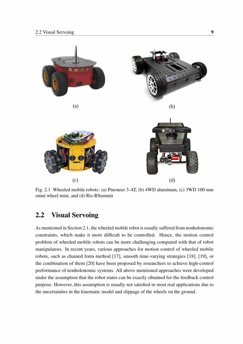
control techniques. Mobile robots are devices that can move from one place to anotherautonomously within a predefined workspace to achieve their desired goals. The mostpopular one among the mobile robots is the wheeled-mobile robot because it is appropriatefor typical applications with relatively low mechanical complexity and energy consumption.Figure 2.1 shows the wheeled mobile robots which are commercially available mobile robotsfor current research.
Despite the simplicity of the kinematic model of a wheeled mobile robot, the design ofstabilizing control laws for this system can be considered a challenge due to the existenceof nonholonomic constraints. The two principal approaches for the problem of controllingnonholonomic systems have been described in [1]. The first approach uses the open-loopcontrol strategies to generate the feasible trajectories and the second one uses the feedbackcontrol strategies to solve the path-following and stabilizing problems. The stabilizingproblem consists in finding adequate feedback control laws that allow the mobile robotto reach a desired state starting from any initial state. Moreover, it needs more elaboratenonlinear techniques. The stabilization problem is a challenging one, because it has beenproven that the kinematic model of a nonholonomic vehicle is open-loop controllable, butnot stabilizable by pure smooth, time-invariant feedback law [2]. This fact makes the controlof nonholonomic systems extremely challenging and stimulates researchers to constructtime-varying or discontinuous feedback controllers for the control of nonholonomic systems.
Many control strategies, such as smooth time-varying strategies [3], [4] and discontinuoustime-invariant control laws have been proposed for various nonholonomic systems [5], [6].Moreover, Tayebi et al. [7] constructed a discontinuous time-invariant feedback controlmethod for n-dimensional nonholonomic chained systems. The switching control and quasi-continuous control based on invariant manifold are proposed for a power system with twoinputs and three states or two inputs and n-states [8], [9]. The quasi-continuous exponentialstabilizing controller that can be applied to both a kinematic-based model and a dynamic-based model was extended [10] to a double integrator form with two inputs and three statesor five states. The switching control based on the invariant manifold assures that all the statessmoothly converge to the origin [11]. Moreover, references [12], [13], [14], and [15] alsoproposed the invariant manifold techniques to control underactuated systems. Lee et al. [16]investigated a parking problem with the point stabilization problem of nonholonomic car-likemobile robots. The algorithm is divided into two steps: stabilization to a desired line andstabilization to a desired point. By using a nonlinear state feedback control law, the steeringoperation is determined.
2.2 Visual Servoing 9
�
(a) (b)
(c) (d)
Fig. 2.1 Wheeled mobile robots: (a) Pinoneer 3-AT, (b) 4WD aluminum, (c) 3WD 100 mmomni wheel mini, and (d) Ris-RSummit
2.2 Visual Servoing
As mentioned in Section 2.1, the wheeled mobile robot is usually suffered from nonholonomicconstraints, which make it more difficult to be controlled. Hence, the motion controlproblem of wheeled mobile robots can be more challenging compared with that of robotmanipulators. In recent years, various approaches for motion control of wheeled mobilerobots, such as chained form method [17], smooth time-varying strategies [18], [19], orthe combination of them [20] have been proposed by researchers to achieve high-controlperformance of nonholonomic systems. All above mentioned approaches were developedunder the assumption that the robot states can be exactly obtained for the feedback controlpurpose. However, this assumption is usually not satisfied in most real applications due tothe uncertainties in the kinematic model and slippage of the wheels on the ground.
10 Background Research
An alternative approach, which can make the feedback loop directly closed at the sensorlayer, has been developed to handle the uncertainties in real environments and improve thecontrol performance of mobile robot systems. Such a strategy is known as the sensor basedcontrol of mobile robots. According to this motivation, a lot of attention has been focused onthe research of visual servoing approaches for mobile robots. In recent years, vision sensorand digital image processing technology become easily available with the development ofcomputer technology. Moreover, vision is an important robotic sensor because it can be usedfor environmental measurements without physical contact. Visual robot control or visualservoing is a feedback control methodology which uses one or more sensors (cameras) tocontrol the motion of the robot. Specifically, the control inputs for the motors used in robotsare produced by processing image data, i.e., they are normally given by extracting contours,features, corners, and other visual primitives. Vision-based control is classified into fourgroups: position-based, image-based, hybrid, and motion-based control system in [21].
The purpose of visual control in robotic manipulators is to control the pose of the robot’send-effector relative to a target object or a set of target features. In mobile robots, the visioncontroller’s task is to control the vehicle’s pose with respect to some landmarks. As shownin Fig. 2.2, there are two basic configurations to perform a visual servoing task in the areaof visual servoing for mobile robots as well as robot manipulators. The camera is rigidlyattached to the mobile base in the eye-in-hand configuration and the camera is fixed on theceiling in the fixed camera configuration.
2.2.1 Position-based visual servoing (PBVS)
The PBVS estimates the position and posture of the robot by matching previous knowledge of3D environmental models with a captured image and controls it directly. Therefore, both ofthe control objective and the control law design are performed in the 3-D Cartesian space inthe PBVS approach. Figure 2.3 shows the block diagram of a position-based visual servoing.
The problems of pose stabilization, following paths, wall following, and vehicle leader-follower were treated by using the position-based visual control in [22], [23], [24], [25], [26]and [27], where the vision systems provide the estimations of the parameters that are neededto implement conventional controllers. The PBVS approach for nonholonomic wheeledmobile robots was presented to reduce the visual servoing task to a control problem in theCartesian space [28], [29], where a pan-tilt camera was used to increase the degrees offreedom of the camera sensor. A piecewise smooth visual feedback control scheme wasproposed to control a nonholonomic cart without the capabilities of dead reckoning [30].A stable vision-based control scheme for nonholonomic vehicle was developed to keepa landmark in the camera field of view [31]. The metrical information about the feature
2.2 Visual Servoing 11
Target
Target
Target
(a)
(b)
Camera
Camera Camera
Target
Camera
Fig. 2.2 Examples of vision-based robot control: (a) eye-in-hand system and (b) fixed camerasystem
position with respect to the camera robot frame is required for all these methods to obtain allof the states for feedback control. Thuilot et al. [32] proposed a control strategy for keepinga moving target object in a field of vision by controlling a Cartesian robot when using thePBVS approach. Ha et al. [33] designed a controller for an eye-in-hand manipulator.
2.2.2 Image-based visual servoing (IBVS)
The IBVS does not need the knowledge of the 3D model of the environment and can operate arobot by controlling only image information which is acquired from a camera image withoutusing the robot position. In the IBVS, both of the control objective and the control law designare directly performed in the image feature parameter space and thus the full model of theobject need not be known accurately. Figure 2.4 shows the block diagram of an image-basedvisual servoing. Compared to PBVS, IBVS can work with faster processing speed and higher
12 Background Research
Cartesian space controller
Robot Camera
Image feature extraction
Desired pose
−
+
Pose estimation
Vid
eo im
age
�
Fig. 2.3 Block diagram of a position-based visual servoing
robustness against camera calibration errors due to the exclusion of the position estimationprocess [34], [35].
An image-based visual servoing approach for the position control of a nonholonomicmobile robot was proposed in [36] to eliminate the dependence on a priori 3-D knowledgeof the scene. In this approach, a discontinuous change of coordinates was used to designa closed-loop stabilizing control law. The image-based visual feedback controller waspresented in [37] to control a mobile robot which can track a moving target of interest,where an adaptive back-stepping was developed to handle the unknown height of the target.Without using any a priori knowledge of the 3-D scene geometry, a new two-step IBVSstrategy was proposed in [38], where an approximate input-output linearizing feedback isused to align the mobile robot with the goal in the first step and then feature points areused to drive the nonholonomic mobile robot to its desired configuration in the second step.Mariottini et al. [39] developed a similar two-step approach using a central catadioptriccamera, which can guarantee the global asymptotic stabilization of nonholonomic mobilerobots to a desired pose. The control schemes in [38] and [39] drove the robot away from thetarget while correcting the lateral error and then the robot was moved backward to the desiredposition to avoid the singularity. The image-based technique has been used in [40], where thedifferential flatness properties are used to generate the most effective path following strategies.In [41], the image-based approach for the path following problem of a mobile robot wasproposed by controlling the shape of the curve in the image plane. The image-based visualservoing techniques for the trajectory tracking and obstacle avoidance of a mobile robot,were developed in [42] and [43]. The image-based fuzzy control approach was developed in[44], where the difference between a reference image and the current image was numericallyexpressed and directly used by a fuzzy control system using a human-like control law. Thealgorithm was applied to control an inverted pendulum system.
2.2 Visual Servoing 13
�
Feature space controller
Robot Camera
Image feature extraction
Desired image
−
+
Vid
eo im
age
Fig. 2.4 Block diagram of an image-based visual servoing
2.2.3 Hybrid visual servoing
The main drawback of 3D visual servoing is that there is no control in the image whichimplies that the target may leave the camera field of view. Moreover, a model of the targetis needed to compute the pose of the camera. The 2D visual servoing does not explicitlyneed this model. However, a depth estimation or approximation is necessary in the design ofthe control law. Furthermore, the main drawback of this approach is that the convergence isensured only in a neighborhood of the desired position. To exploit the respective advantagesof PBVS and IBVS approaches, a hybrid visual servoing scheme was first proposed in [45].The hybrid approach is also called 2.5-D visual servoing in the literature, and its controlobjective and control law design are implemented both in the 3-D Cartesian space and inthe 2-D image space. To remove the dependence on the exact knowledge of object models,homography calculation and decomposition are carried out to obtain the 3-D informationused by the 2.5-D visual servoing scheme. Figure 2.5 shows the block diagram of a hybridvisual servoing.
In [46], Murrieri et al. developed a hybrid control approach for the parking problem of anonholonomic mobile robot, where the visual feedback from low-cost cameras is only usedfor the stabilization of the vehicle to a given position and orientation. This approach cansuccessfully keep the features in the camera field of view during the visual servoing process.To design the visual servoing scheme for unicycle mobile robots, the 2.5-D control schemewas proposed in [47].
2.2.4 Motion-based visual servoing
The recently developed visual servoing technique was a motion-based visual servoing. Itis also called a model-free vision-based control technique because the optical flow in theimage can be measured without having any a priori knowledge of the target. In this approach,
14 Background Research
�
Controller Robot Camera
Image feature extraction
−
+
Projective reconstruction
Vid
eo im
age
Reference image
0
Fig. 2.5 Block diagram of a hybrid visual servoing
Controller Robot Camera
Motion extraction
Reference motion
−
+
Vid
eo im
age
�
Fig. 2.6 Block diagram of a motion-based visual servoing
the error, which is used to compute the control law, is calculated as a function of the opticalflow measured in the image and a reference optical flow which should be obtained by thesystem. This approach is suitable for the tasks such as the contour tracking [48], cameraself-orientation and docking [49], and the application to control an eye-in-hand system inorder to position the image plane parallel to a target plane [50]. There is a high servoingrate, which imposes the velocity of the small robot. This fact becomes the major problemof the motion-based visual servoing. However, the developments in the motion estimationalgorithms will give the solutions which can make a faster visual control loop. Figure 2.6shows the block diagram of a motion-based visual servoing.
2.3 Mobile Robot Control Using Fuzzy Logic
Fuzzy control systems have found a wide range of applications in many fields of science andtechnology such as identification, planning, and model-free control of complex nonlinearsystems. Fuzzy control was introduced with the proposal of fuzzy set theory by Prof. Lotfi
2.3 Mobile Robot Control Using Fuzzy Logic 15
Fuzzy inference mechanism
Fuzzy rule
Fuzz
ific
atio
n
Def
uzzi
fica
tion
Mobile robot
ReferenceInputr(t)
Errore(t)
Control signalu(t)
Outputy(t)
−
+
Fig. 2.7 Basic fuzzy mobile robot control loop
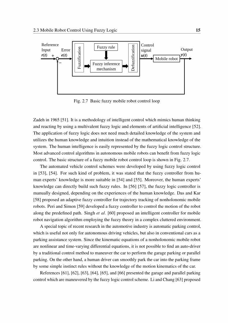
Zadeh in 1965 [51]. It is a methodology of intelligent control which mimics human thinkingand reacting by using a multivalent fuzzy logic and elements of artificial intelligence [52].The application of fuzzy logic does not need much detailed knowledge of the system andutilizes the human knowledge and intuition instead of the mathematical knowledge of thesystem. The human intelligence is easily represented by the fuzzy logic control structure.Most advanced control algorithms in autonomous mobile robots can benefit from fuzzy logiccontrol. The basic structure of a fuzzy mobile robot control loop is shown in Fig. 2.7.
The automated vehicle control schemes were developed by using fuzzy logic controlin [53], [54]. For such kind of problem, it was stated that the fuzzy controller from hu-man experts’ knowledge is more suitable in [54] and [55]. Moreover, the human experts’knowledge can directly build such fuzzy rules. In [56] [57], the fuzzy logic controller ismanually designed, depending on the experiences of the human knowledge. Das and Kar[58] proposed an adaptive fuzzy controller for trajectory tracking of nonholonomic mobilerobots. Peri and Simon [59] developed a fuzzy controller to control the motion of the robotalong the predefined path. Singh et al. [60] proposed an intelligent controller for mobilerobot navigation algorithm employing the fuzzy theory in a complex cluttered environment.
A special topic of recent research in the automotive industry is automatic parking control,which is useful not only for autonomous driving vehicles, but also in conventional cars as aparking assistance system. Since the kinematic equations of a nonholonomic mobile robotare nonlinear and time-varying differential equations, it is not possible to find an auto-driverby a traditional control method to maneuver the car to perform the garage parking or parallelparking. On the other hand, a human driver can smoothly park the car into the parking frameby some simple instinct rules without the knowledge of the motion kinematics of the car.
References [61], [62], [63], [64], [65], and [66] presented the garage and parallel parkingcontrol which are maneuvered by the fuzzy logic control scheme. Li and Chang [63] proposed
16 Background Research
the experimental studies on fuzzy garage-parking control and fuzzy parallel-parking controlusing a car-like mobile robot, where the CCD camera was used for the overall vision of thecar park, but it is an expensive method. For the experimental study of fuzzy garage parkingcontrol, Li et al. [64] adopted the six infrared sensors to measure the distances betweenthe robot and the surroundings, and [65] used the sensor fusion techniques to combine theultrasonic sensors, encoders, and gyroscopes with a differential GPS system to detect andestimate the dimensions of the parking lot. The new intelligent auto-parking system wasdescribed in [67], where the fuzzy-logic based trajectory generation algorithm was used forparallel parking without collisions. The problem of parallel and diagonal parking of wheeledvehicles was developed in [68], where the fuzzy logic was used to select the most suitablemanoeuvre from the solution set according to the environment, dealing with optimality, pathtracking performance and collision avoidance trade-off.
Daxwanger [69] proposed a skilled-based visual parking control using neural networksand fuzzy, where two control architectures, the direct neural control and the fuzzy hybridcontrol, were used to generate the automatic parking commands. A video sensor was used tomeasure the environment and the control architectures were validated by experiments withan autonomous mobile robot. For parking control, the state evaluation fuzzy control and thepredictive fuzzy control were exploited to achieve the drive knowledge in [70]. In [71], thefuzzy traveling control of a mobile robot with the six supersonic sensors has been proposed,where the flush problem was considered. For maneuvering the vehicle in the parking lot, thedevelopment of a near-optimal fuzzy controller has been provided in [72]. The membershipfunctions and rules of the fuzzy controller were generated by using the statistical propertiesof the individual trajectory groups. For parallel parking control of the car-like mobile robot,a fuzzy gain scheduling controller was investigated in [73], where a fuzzy sliding modecontroller was firstly used to locally track a typical path. Several typical paths were formedto complete the parallel parking procedure.
2.4 Optimized Fuzzy Controller by Genetic Algorithms
In most fuzzy systems, membership functions, fuzzy reasoning rules and scaling factorsare determined through trial and error by human operators, and it takes many iterations toconverge to desirable parameters. Many researchers have explored the use of GAs to tunefuzzy logic controllers in order to optimize the parameters of them [74], [75]. The basicconcepts of GA were introduced in [76] and his work was developed in the several researchworks [77]. GA is a robust optimization technique and does not need any prior information
2.4 Optimized Fuzzy Controller by Genetic Algorithms 17
Chromosome
Chromosome
Evaluation
Solutions
Selection
Crossover
Mutation
Best chromosome
Best solution
End i = i+1N
Y
decoding
encoding
Nex
t gen
erat
ion
ith population
�
Fig. 2.8 Genetic algorithm flowchart
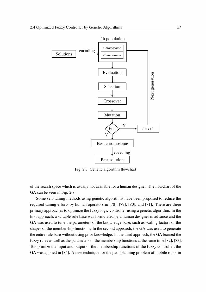
of the search space which is usually not available for a human designer. The flowchart of theGA can be seen in Fig. 2.8.
Some self-tuning methods using genetic algorithms have been proposed to reduce therequired tuning efforts by human operators in [78], [79], [80], and [81]. There are threeprimary approaches to optimize the fuzzy logic controller using a genetic algorithm. In thefirst approach, a suitable rule base was formulated by a human designer in advance and theGA was used to tune the parameters of the knowledge base, such as scaling factors or theshapes of the membership functions. In the second approach, the GA was used to generatethe entire rule base without using prior knowledge. In the third approach, the GA learned thefuzzy rules as well as the parameters of the membership functions at the same time [82], [83].To optimize the input and output of the membership functions of the fuzzy controller, theGA was applied in [84]. A new technique for the path planning problem of mobile robot in
18 Background Research
static environment was developed by using the combination of fuzzy logic, GA and NeuralNetworks (NN) in [85].
In order to improve the automatic parallel parking performance, Azadi and Taherkhani[86] optimized the fuzzy membership functions using a GA based on heuristic rules. In [87],the GA was used to optimize the parameters of the membership functions and scaling factorsof fuzzy systems for parallel parking. To improve the conventional GAs in designing fuzzycontrollers, a new context-dependent coding technique, chromosome reordering operators,and the coevolution of controller testing sets, were developed in [88]. The algorithm wasapplied to the parallel parking control of a mobile robot.
2.5 Summary
This chapter presented a thorough investigation in the areas of controlling of the car-likemobile robot. Several research gaps in the areas of designing parking controllers wereidentified through detailed examination.
Chapter 3
Invariant Manifold-based StabilizingControllers for Parking Problems
The car-like mobile robots are highly nonlinear, and especially nonholonomic constraintshave motivated the development of highly nonlinear control techniques. A system withnonholonomic constraints attracts its attention from the viewpoint of control theory becauseno conventional control can be applied directly to such a system. Since it cannot be stabilizedby a static continuous feedback with gains, there are several control methods by using achained form up to now. The point-stabilizing controllers for various nonholonomic systemshave been proposed in many recent works. However, their research studies are all about thestabilizing problem at the origin.
This chapter presents the new stabilizing controllers based on invariant manifold theoryfor point-to-point control (parking problems), which allow the car-like mobile robot toreach the desired pose starting from any initial pose. Note here that the combination of theposition and orientation is referred to as the pose of the robot. The stability of the proposedcontrol system is analyzed using Lyapunov theory. The car-like mobile robot which is anunderactuated system with two inputs is considered as a controlled object. The switchingand non-switching control methods based on an invariant manifold theory are proposed forstabilizing it in the desired pose, where a chained form model is assumed to be used as acanonical model.
The rest of this chapter is organized as follows. Section 3.1 describes the problem settingwe are concerned with and Section 3.2 provides the construction of invariant manifoldtheory. Section 3.3 provides the attractive control based on this as well as the switching andnon-switching control laws. The several simulation results are presented to demonstrate ourtheoretical results in Section 3.4. Section 3.5 summarizes the chapter.
20 Invariant Manifold-based Stabilizing Controllers for Parking Problems
3.1 Problem Setting
x
y
θ
ϕ
l
s
(x, y)
Fig. 3.1 Configuration of a car-like mobile robot
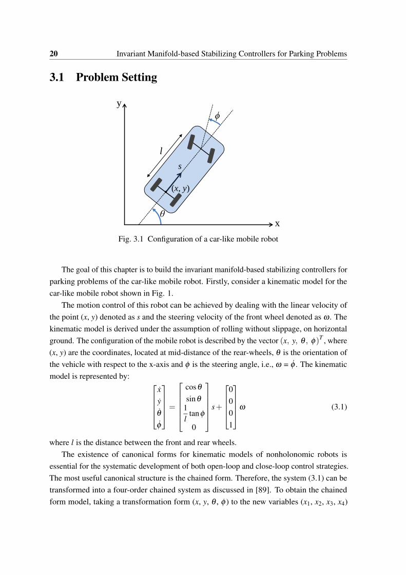
The goal of this chapter is to build the invariant manifold-based stabilizing controllers forparking problems of the car-like mobile robot. Firstly, consider a kinematic model for thecar-like mobile robot shown in Fig. 1.
The motion control of this robot can be achieved by dealing with the linear velocity ofthe point (x, y) denoted as s and the steering velocity of the front wheel denoted as ω . Thekinematic model is derived under the assumption of rolling without slippage, on horizontalground. The configuration of the mobile robot is described by the vector (x, y, θ , φ)T , where(x, y) are the coordinates, located at mid-distance of the rear-wheels, θ is the orientation ofthe vehicle with respect to the x-axis and φ is the steering angle, i.e., ω = φ . The kinematicmodel is represented by:
xyθ
φ
=
cosθ
sinθ
1l
tanφ
0
s+
0001
ω (3.1)
where l is the distance between the front and rear wheels.The existence of canonical forms for kinematic models of nonholonomic robots is
essential for the systematic development of both open-loop and close-loop control strategies.The most useful canonical structure is the chained form. Therefore, the system (3.1) can betransformed into a four-order chained system as discussed in [89]. To obtain the chainedform model, taking a transformation form (x, y, θ , φ ) to the new variables (x1, x2, x3, x4)
3.1 Problem Setting 21
throughx1 = x
x2 =tanφ
lcos3θ
x3 = tanθ
x4 = y
(3.2)
together with the input transformation.
s =u1
cosθ
ω =−3cos2φ tanθ tan2φ
l cosθu1 + lcos2
φcos3θu2
(3.3)
The (2,4) chained model becomesx1 = u1
x2 = u2
x3 = x2u1
x4 = x3u1
(3.4)
where u1 and u2 are the control inputs for the canonical model.Since our aim of this chapter is to derive the controllers for stabilizing the car-like mobile
robot in the desired pose, the robot is assumed that it can move from any given initial pose tothe desired pose. The desired variables (x1d , x2d , x3d , x4d) in the chained form are defined asfollows:
x1d = xd
x2d =tanφd
lcos3θdx3d = tanθd
x4d = yd
(3.5)
where (xd,yd,θd,φd)T denotes the desired state vector in the original model. Firstly, define
the error signal e such as:e1 , x1 − x1d
e2 , x2 − x2d
e3 , x3 − x3d +α
e4 , x4 − x4d +β
(3.6)
22 Invariant Manifold-based Stabilizing Controllers for Parking Problems
Then, it is easy to note that the time derivatives of the error signals e1 and e2 are given by
e1 = x1 = u1
e2 = x2 = u2
(3.7)
and the derivative of e3 becomes
e3 = x3 + α
= x2u1 + α = x2u1 − x2du1 + x2du1 + α
= e2u1 + x2du1 + α
(3.8)
We want to satify α =−x2du1 to obtain e3 = e2u1. Then, u1 = e1 and α =−x2d e1, so thatwe choose α =−x2de1 and then
e3 = x3 − x3d − x2de1 (3.9)
Along the same way as made in above, it follows that
e4 = x4 + β
= x3u1 + β = u1 (e3 + x3d −α)+ β
= e3u1 + x3du1 + x2de1u1 + β
(3.10)
We choose β = −(x3d + x2de1)u1 from Eq. (3.10) to obtain e4 = e3u1. Then u1 = e1 and
β =−(x3d + x2de1) e1, finally we choose β =−x3de1 −12
x2de21 and then
e4 = x4 − x4d − x3de1 −12
x2de21 (3.11)
In this chapter, three types of switching controllers which perform two steps of control byan invariant manifold, and the non-switching controller are derived for parking problems ofthe car-like mobile robot. In the switching control technique, attractive control to an invariantmanifold is performed first in the first step, and each state on the invariant manifold is stabi-lized in the second step. In the non-switching approach, the manifold will be automaticallyattractive by means of an additional state feedback, namely, v.
3.2 Derivation of Invariant Manifold 23
3.2 Derivation of Invariant Manifold
Firstly, recall the definition of invariant manifold. According to the introduction to a mobilerobot control’s book [90].
DEFINITION 1. An invariant manifold is an invariant set that happens to be a differ-entiable manifold. More specially, let S : Rn → Rm be a smooth map. A manifold M =
{xxx ∈ Rn : S (xxx) = 0} is invariant for the dynamic system xxx = f (xxx, uuu) if all system trajecto-ries in M at t = t0 remain in this manifold for all t ≥ t0. In other words, the Lie derivativeof S along the vector field f is zero (L f S (xxx) = 0) for all xxx ∈ M.
DEFINITION 2. An invariant manifold M = {xxx ∈ Rn : S (xxx) = 0} is said to be an attractivemanifold in an open domain X of Rn, where X ∈ M, if for all such that t0 ≥ 0 such thatx(t0) ∈ X , then limt→∞ x(t) ∈ M which implies that any x(t0) outside M is always attractedtoward M.
Note, however, that invariant manifold M of xxx = f (xxx, uuu) should be held for stabilizinginput uuu which is assumed to be linear state feedback control uuu =−kxxx. Our aim is to derive astable invariant manifold which stabilizes the following controlled object:
e1 = u1
e2 = u2
e3 = e2u1
e4 = e3u1
(3.12)
and consider a stabilizing control problem such that eee(t) = [e1, e2, e3, e4]T become zero as
t → ∞. Here, all the states are assumed to be measurable.To derive a stable invariant manifold, the following linear feedback is applied to Eq. (3.12):
u1 =−ke1
u2 =−ke2
(3.13)
where k > 0 is a linear feedback gain.The closed-loop time response e1 (t) and e2 (t) are derived as follows:
e1 (t) = e1 (0)e−kt
e2 (t) = e2 (0)e−kt(3.14)

24 Invariant Manifold-based Stabilizing Controllers for Parking Problems
so thate3 (t) =−e2 (0)e−ktke1 (t) =−ke2 (0)e−kte1 (0)e−kt
=−ke1 (0)e2 (0)e−2kt(3.15)
e3 (t) = e3 (0)+[
12
e1 (0)e2 (0)e−2kt]t
0
= e3 (0)−12
e1 (0)e2 (0)+12
e1 (0)e2 (0)e−2kt(3.16)
and
e4 =−[
e3 (0)−12
e1 (0)e2 (0)+12
e1 (0)e2 (0)e−2kt]
ke1
=−[
e3 (0)−12
e1 (0)e2 (0)+12
e1 (0)e2 (0)× e−2kt]
ke1 (0)e−kt
=−k[
e1 (0)e3 (0)e−kt − 12
e21 (0)e2 (0)e−kt +
12
e21 (0)e2 (0)e−3kt
] (3.17)
e4 (t) = e4 (0)+[
e1 (0)e3 (0)e−kt − 12
e21 (0)e2 (0)e−kt +
16
e21 (0)e2 (0)e−3kt
]t
0
= e4 (0)− e1 (0)e3 (0)+12
e21 (0)e2 (0)−
16
e21 (0)e2 (0)+ e1 (0)e3 (0)e−kt
−12
e21 (0)e2 (0)e−kt +
12
e21 (0)e2 (0)e−3kt
(3.18)
As one candidate of the invariant manifold, S (eee) can be selected from the constant terms ofe4 (t) such as
S (eee) = e4 (t)− e1 (t)e3 (t)+13
e21 (t)e2 (t) (3.19)
In fact, S (eee) can be reduced, under the feedback control given by Eq. (3.12), to
S (eee) = e4 (t)− e1 (t)e3 (t)− e1 (t) e3 (t)+23
e1 (t)e1 (t)e2 (t)+13
e21 (t) e2 (t)
= e3u1 −u1e3 − e1e2u1 +23
e1e2u1 +13
e21u2
=−13
e1e2u1 +13
e21u2 =
13
ke21e2 −
13
ke21e2
≡ 0
(3.20)
That is S (eee) = constant. Clearly, once error of the system state reaches a manifold with aconstant = 0 (i.e., S (eee) = 0) then by Eq. (3.19) the entire error of state eee(t) = [e1, e2, e3, e4]
T
tends to zero exponentially. Therefore, S (eee) is an invariant manifold for our controlled systemEq. (3.12) under the feedback control law Eq. (3.13). Furthermore, from Eq. (3.12) and
3.3 Attractive Control to the Manifold 25
Eq. (3.13), it follows that
e1 (t) =−ke1, e2 (t) =−ke2
so that e1 (t) and e2 (t) are asymptotically stable, i.e., e1 → 0 and e2 → 0 as t → ∞. Then, itis true that e4 → 0 because of S (eee) = 0. Additionally, it is found from Eq. (3.16) that e3 → 0if e2 (0) = e3 (0) = 0 for ∀e1 (0).
3.3 Attractive Control to the Manifold
An attractive controller is described here to the manifold derived in the previous section. Toobtain the first-step control law for realizing S (eee) = 0, we select the Lyapunov function ofS (eee) as
V (eee) = 12S2 (eee) (3.21)
3.3.1 Switching controller I
First, set the control input as
u1 = f S (eee(t))e2 (t)e1 (t)
u2 =− f S (eee(t))(3.22)
where f denotes the feedback gain for the attractive control. Then, it follows that
V (eee) = SS = S(−1
3e1e2u1 +
13
e21u2
)=−1
3S(
f Se22 + f Se2
1)
=−13
f S2W (eee)≤ 0
(3.23)
where,W (eee), e2
1 (t)+ e22 (t) (3.24)
Note here that, under the control law of Eq. (3.22), this W (eee) becomes
W = 2e2e2 +2e1e1
= 2e2u2 +2e1u1 ≡ 0(3.25)
26 Invariant Manifold-based Stabilizing Controllers for Parking Problems
Namely, it is seen that W (eee(t)) =W (eee(0)). Therefore, Eq. (3.23) becomes negative definite,so that S (eee)→ 0 as t → ∞, as long as W (eee(0)) = 0.This controller is not implementable forthe case of e1 (0) = 0 and e2 (0) = 0 , in which the controller makes the system unstable.
3.3.2 Switching controller II
As the second candidate, set the control input as
u1 = f S (eee)e1 (t)e2 (t)
u2 =− f S (eee)e22 (t)
(3.26)
Along the same way as made in above, it follows that
V (eee) = SS = S(−1
3e1e2u1 +
13
e21u2
)=−1
3S(
f Se21e2
2 + f Se21e2
2)
=−23
f S2W (eee)≤ 0
(3.27)
where,W (eee), e2
1 (t)e22 (t) (3.28)
Note here that, under the control law of Eq. (3.26), this W (eee) becomes
W = 2(e21e2e2 + e2
2e1e1)
= 2(e21e2u2 + e2
2e1u1)≡ 0(3.29)
Namely, it is seen that W (eee(t)) =W (eee(0)). Therefore, Eq. (3.27) becomes negative definite,so that S (eee)→ 0 as t → ∞, as long as W (eee(0)) = 0.This controller is not implementable forthe case of e1 (0) = 0 or e2 (0) = 0 , in which the controller makes the system unstable.
3.3.3 Switching controller III
As the third candidate, set the control input as
u1 = f S (eee)e1 (t)e2 (t)
u2 =− f S (eee) , f > 0(3.30)
3.3 Attractive Control to the Manifold 27
It follows that
V (eee) = SS = S(−1
3e1e2u1 +
13
e21u2
)=−1
3S(
f Se21 + f Se2
1)
=−23
f S2W (eee)≤ 0
(3.31)
where,W (eee), e2
1 (t) , e1 (0) = 0 (3.32)
3.3.4 Non-switching controller
In the previous section, we found that there is a limitation for vehicle orientation due to theincomplete manifold in the system. Therefore we enhance the linear state feedback controllerto make the constructed manifold attractive with the method of Tayebi et al [7], where notethat they originally dealt with the stabilization of a three-wheeled mobile robot at the origin.
In this subsection, we design the stabilizing controller for parking problems which allowthe car-like mobile robot to reach a desired pose starting from any initial pose. Here, twomanifolds are introduced: one is coming from the non-zero constants of the solution to e3 (t),whereas the other is coming from those of the solution to e4 (t). That is, the following twomanifolds are defined:
S1 (t) = e3 (t)−12
e1 (t)e2 (t)
S2 (t) = e4 (t)− e1 (t)e3 (t)+13
e21 (t)e2 (t)
(3.33)
where S2 (t)≡ S (t). It is easy to see that S1 (t) is an invariant manifold under the control lawgiven in Eq. (3.13).
The transformation from (e1,e2,e3,e4) to (e1,e2,S1,S2) is a diffeomorphism, so that thestabilization of (e1,e2,e3,e4) is equivalent to the stabilization of (e1,e2,S1,S2). Therefore,to stabilize the system (3.12), it is sufficient to lend (e1,e2,e3, e4) into a manifold by anadditional state feedback, that is, to make the manifold attractive. In the sequel, a new
28 Invariant Manifold-based Stabilizing Controllers for Parking Problems
controlled objective is reconsidered by
e1 = u1
e2 = u2
S1 =12
e2u1 −12
e1u2
S2 =−13
e1e2u1 +13
e21u2
(3.34)
The enhanced controller to be used in Eq. (3.34) is assumed to be given by
u1 =−ke1, u2 =−ke2 + v (3.35)
where v is a control term added to the u2 channel. Then, the closed-loop system is reduced to
e1 =−ke1
e2 =−ke2 + v
S1 =−12
ke1e2 +12
ke1e2 −12
e1v
=−12
e1v
S2 =13
ke21e2 −
13
ke21e2 +
13
e21v
=13
e21v
(3.36)
The system of the last two equations in Eq. (3.36) can be written as:
SSS = E (e1)bbbv, SSS =[S1 S2
]T(3.37)
where,
E (e1) =
[e1 0
0 e21
], bbb =
−12
13
(3.38)
Now, introducing a transformed variable zzz:
zzz = E−1 (e1)SSS (3.39)
3.4 Simulation Experiments 29
which is valid for e1 = 0, it is found that
zzz =ddt
E−1 (e1)SSS+E−1 (e1) SSS
=
−e1
e21
0
0 −2e1
e31
E (e1)zzz+bbbv
=
ke1
0
02ke2
1
E (e1)zzz+bbbv
(3.40)
that iszzz = Azzz+bbbv (3.41)
where,
A =
[k 0
0 2k
](3.42)
The system given by Eq. (3.41) can be stabilized by using a feedback controller of the form:
v =−gggzzz, ggg =[g1 g2
](3.43)
Using Eq. (3.43), the closed-loop system becomes
zzz = Aczzz (3.44)
whereAc , A−bbbggg (3.45)
In this approach, the manifold will be automatically attractive by means of an additional statefeedback, namely, v.
3.4 Simulation Experiments
Simulation results are presented here to demonstrate the ability of the proposed controllers toconverge the car-like mobile robot to the desired poses. All the controllers I to IV derived inthe previous section were set in the first step, but the linear controllers given in Eq. (3.13)were set in the second step as a switching approach.
30 Invariant Manifold-based Stabilizing Controllers for Parking Problems
(a)
(b)
0 1 2 3 4 5-4
-3
-2
-1
0
1
2
3
Time t [s]
Stat
es x
[m
], y
[m
], θ
[ra
d], a
nd φ
[ra
d]
x yθφ
0 1 2 3 4 5-25
-20
-15
-10
-5
0
5
Time t [s]
Inpu
ts s
[m/s
] an
d ω
[ra
d/s]
s
ω
Fig. 3.2 Control results using the switching controller I: (a) state responses and (b) controlinputs
As stated the above sections, our objective is to drive the car-like mobile robot from anygiven initial pose to the desired pose. To compare the effectiveness of each controller forbackward parallel parking clearly, the same initial and desired states are set for all controllers.However, for switching controllers I, II and III, the initial states are set as x(0) = 2 m,y(0) = 2 m, θ (0) = 1.0 rad, and φ (0) = 0.523 rad because the vehicle will go to undesiredstates if the initial orientation is not equal 1 radian and steering angle equal zero. In this
3.4 Simulation Experiments 31
-5 0 5 10x-coordinate x [m]
Desired (-3, -1.7, 0, 0)
Start (2, 2, 1.0, 0.523)
y-co
ordi
nate
y [
m]
-5
0
6
Fig. 3.3 Backward parallel parking result using the switching controller I
simulation studies, the desired states are set as xd =−3.0 m, yd =−1.7 m, θd = 0 rad, andφd = 0 rad for all controllers.
Figure 3.2 (a) and (b) show the convergence of the whole states of system (3.1) and thetime evolution of the control variables for the controllers I. The simulation result of backwardparallel parking using the switching controller I is illustrated in Fig. 3.3, where the vehicleorientation converged to a non-desired value about 0.275 rad. Here, it was assumed that thewheelbase of the car-like mobile robot was l = 2.5 [m], the sampling width was ∆t = 0.01 [s],the control gains were set to k = 2 and f = 1 and the threshold for the switching ε = 1/1000.
The convergence of the whole states and the time evolution of the control variables forthe switching controllers II and III, are shown in Figs. 3.4 and 3.6. The simulation results ofbackward parallel parking using the switching controllers II and III are illustrated in Figs.3.5 and 3.7. It is found that all the vehicle positions converged to the desired states ideally.However, the vehicle orientations converged to undesired ones if the initial orientation wasnot 1 radian.
Finally, the simulation results for the backward parallel parking when using a non-switching rule given in Eqs. (3.35) and (3.43) are given in Figs. 3.8 and 3.9, under thecondition of x(0) = 2 m, y(0) = 2 m, θ (0) = 0 and φ (0) = 0. Here, when defining k = 2,the gain vector was determined as ggg = [20 63] to make the eigenvalues of (A−bbbggg) equal to−2 and −3. It is seen from Figs. 3.8 and 3.9 that this approach assures that all the states
32 Invariant Manifold-based Stabilizing Controllers for Parking Problems
(a)
(b)
0 1 2 3 4 5
-2
0
2
4
6
Time t [s]
Stat
es x
[m
], y
[m
], θ
[ra
d], a
nd φ
[ra
d]
x yθφ
0 1 2 3 4 5
-50
0
50
100
Time t [s]
Inpu
ts s
[m/s
] an
d ω
[ra
d/s]
s
ω
Fig. 3.4 Control results using the switching controller II: (a) state responses and (b) controlinputs
converge to the desired states, even if the vehicles starts from any initial state, unlike theswitching approach. Note however that this controller everytime gives very large initial ω
due to a linear pole-allocation. In fact, ω was assumed to be restricted such as |ω| ≤ 2.5π
[rad/s].Our controllers are tested for forward parallel parking too. The comparison of the vehicle
orientation errors for forward parallel parking of each controller is shown in Fig. 3.10. Asshown in this figure, there was no vehicle orientation error for non-switching approach.
3.5 Summary 33
�
Desired (-3, -1.7, 0, 0)
Start (2, 2, 1.0, 0.523)
-5 0 5 10x-coordinate x [m]
y-co
ordi
nate
y [
m]
-5
0
5
10
Fig. 3.5 Backward parallel parking result using the switching controller II
The orientation errors for the switching controllers II and III will become zero if the initialorientation is 1 radian. However, it still had the orientation error for the switching controllerI, even if the initial orientation was 1 radian. Figure 3.11 shows the comparison of the vehicleorientation errors for backward parallel parking of each controller.
3.5 Summary
The simulation results show the effectiveness of the proposed controllers. When the initialorientation and steering angle were θ = 1 radian and φ = 0 respectively, the switchingcontrollers II and III converged the vehicle to the desired states for both forward and backwardparallel parking. If not the case its orientation converged to undesired one. It is attributedto the fact that the manifold derived in Eq. (3.19) has an undesirable limitation as shownin Section 3.3. For the switching controller I, there is a small amount of orientation errorabout −0.275 rad even we set the same initial orientation and steering angle values with the
34 Invariant Manifold-based Stabilizing Controllers for Parking Problems
(a)
(b)
0 1 2 3 4 5
-2
0
2
4
6
Time t [s]
Stat
es x
[m
], y
[m
], θ
[ra
d], a
nd φ
[ra
d]
x yθφ
0 1 2 3 4 5-60
-40
-20
0
20
40
60
Time t [s]
Inpu
ts s
[m/s
] an
d ω
[ra
d/s]
s
ω
Fig. 3.6 Control results using the switching controller III: (a) state responses and (b) controlinputs
switching controllers II and III. On the other hand, it has been proved that the car-like mobilerobot was able to be stable and converged to a desired pose for both parking types by using anon-switching controller.
In this chapter, the several stabilizing controllers have been proposed for parking problemsof the car-like mobile robot that was an under-actuated system with two inputs and fouroutputs. Especially, after obtaining a chained form, invariant manifolds were derived basedon such a model to design the switching and non-switching controllers for stabilizing of the
3.5 Summary 35
�
Desired (-3, -1.7, 0, 0)
Start (2, 2, 1.0, 0.523)
-5 0 5 10x-coordinate x [m]
y-co
ordi
nate
y [
m]
-5
0
5
10
Fig. 3.7 Backward parallel parking result using the switching controller III
car-like mobile robot in the parking system. Some computer simulation results were given toillustrate the effectiveness of the proposed controllers.
36 Invariant Manifold-based Stabilizing Controllers for Parking Problems
(a)
(b)
0 1 2 3 4 5-5
0
5
Time t [s]
Stat
es x
[m
], y
[m
], θ
[ra
d], a
nd φ
[ra
d]
x yθφ
0 1 2 3 4 5-10
-8
-6
-4
-2
0
2
4
Time t [s]
Inpu
ts s
[m/s
] an
d ω
[ra
d/s]
s
ω
Fig. 3.8 Control results using a non-switching controller: (a) state responses and (b) controlinputs
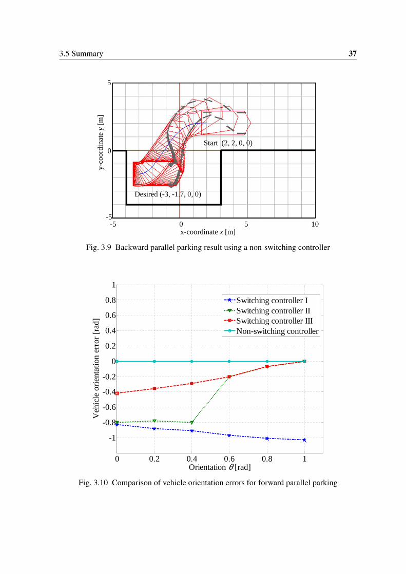
3.5 Summary 37
�
-5 0 5 10x-coordinate x [m]
Desired (-3, -1.7, 0, 0)
Start (2, 2, 0, 0)
y-co
ordi
nate
y [
m]
-5
0
5
Fig. 3.9 Backward parallel parking result using a non-switching controller
0 0.2 0.4 0.6 0.8 1
-1
-0.8
-0.6
-0.4
-0.2
0
0.2
0.4
0.6
0.8
1
Orientation θ [rad]
Veh
icle
ori
enta
tion
erro
r [r
ad]
Switching controller ISwitching controller IISwitching controller IIINon-switching controller
Fig. 3.10 Comparison of vehicle orientation errors for forward parallel parking
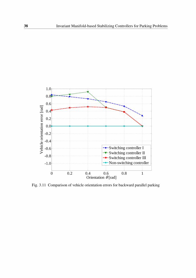
38 Invariant Manifold-based Stabilizing Controllers for Parking Problems
0 0.2 0.4 0.6 0.8 1
-1.0
-0.8
-0.6
-0.4
-0.2
0.0
0.2
0.4
0.6
0.8
1.0
Orientation θ [rad]
Veh
icle
ori
enta
tion
erro
r [r
ad]
Switching controller ISwitching controller IISwitching controller IIINon-switching controller
Fig. 3.11 Comparison of vehicle orientation errors for backward parallel parking
Chapter 4
Image-based Fuzzy Parking Control of aCar-like Mobile Robot
The stabilizing controllers for the parking problems of a car-like mobile robot were consideredin the previous chapter. However, it was assumed that the robot states can be exactly obtainedfor the feedback control purpose. In most real applications, it will not be satisfied due tothe uncertainties in the kinematic model and slippage of the wheels on the ground. For thisreason, we are interested in a vision-based control method in our future tasks.
Automatic parking system is one of the interesting topics in developing intelligentvehicles. However, if the parking controller is not designed properly, it may endanger thevehicle and the driver. This chapter presents a novel image-based fuzzy controller whichcan automatically drive the car-like mobile robot equipped with a web camera toward aparking frame which is drawn on the floor. The image-based control method can operate amobile robot by controlling only image information acquired from camera images withoutusing the robot states. The proposed system consists of two parts. In the first part, a robotequipped with a web camera detects a red color parking frame which are drawn on the floorand generates the desired target line to be followed by the robot using a Hough transform. Afuzzy controller is designed with two inputs, which are the slope and intercept of the targetline, and one output that is the steering angle of the robot to complete a parking task, in thesecond part.
The rest of this chapter is organized as follows. In Section 4.1, the problem setting isassigned. In Section 4.2, the parking lines on the floor are detected from a robot equippedwith a web camera and a target line for an automatic parking system is generated from acaptured image by using an image processing technique with a Progressive ProbabilisticHough Transform (PPHT). Section 4.3 provides the fuzzy controller to follow such a target
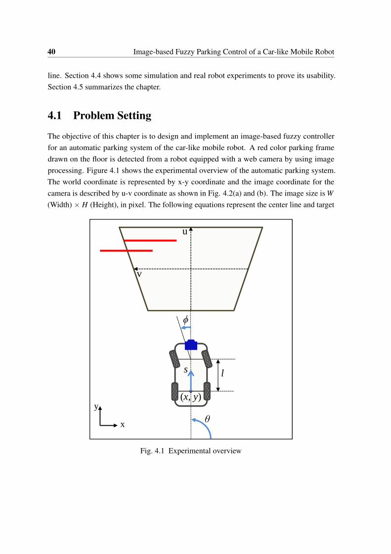
40 Image-based Fuzzy Parking Control of a Car-like Mobile Robot
line. Section 4.4 shows some simulation and real robot experiments to prove its usability.Section 4.5 summarizes the chapter.
4.1 Problem Setting
The objective of this chapter is to design and implement an image-based fuzzy controllerfor an automatic parking system of the car-like mobile robot. A red color parking framedrawn on the floor is detected from a robot equipped with a web camera by using imageprocessing. Figure 4.1 shows the experimental overview of the automatic parking system.The world coordinate is represented by x-y coordinate and the image coordinate for thecamera is described by u-v coordinate as shown in Fig. 4.2(a) and (b). The image size is W(Width) × H (Height), in pixel. The following equations represent the center line and target
�
ϕ
θ
u
v
x
y
l
(x, y)
s
Fig. 4.1 Experimental overview
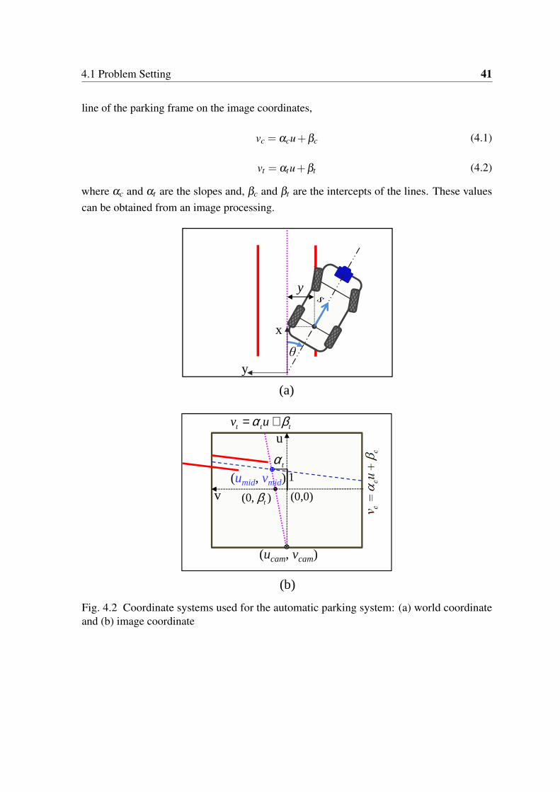
4.1 Problem Setting 41
line of the parking frame on the image coordinates,
vc = αcu+βc (4.1)
vt = αtu+βt (4.2)
where αc and αt are the slopes and, βc and βt are the intercepts of the lines. These valuescan be obtained from an image processing.
�
x
y
y
θ
v (0,0)
u
1tα
(0, )tβ
t t tv uα β= +
(a)
(b)
(umid, vmid)
(ucam, vcam)
Fig. 4.2 Coordinate systems used for the automatic parking system: (a) world coordinateand (b) image coordinate
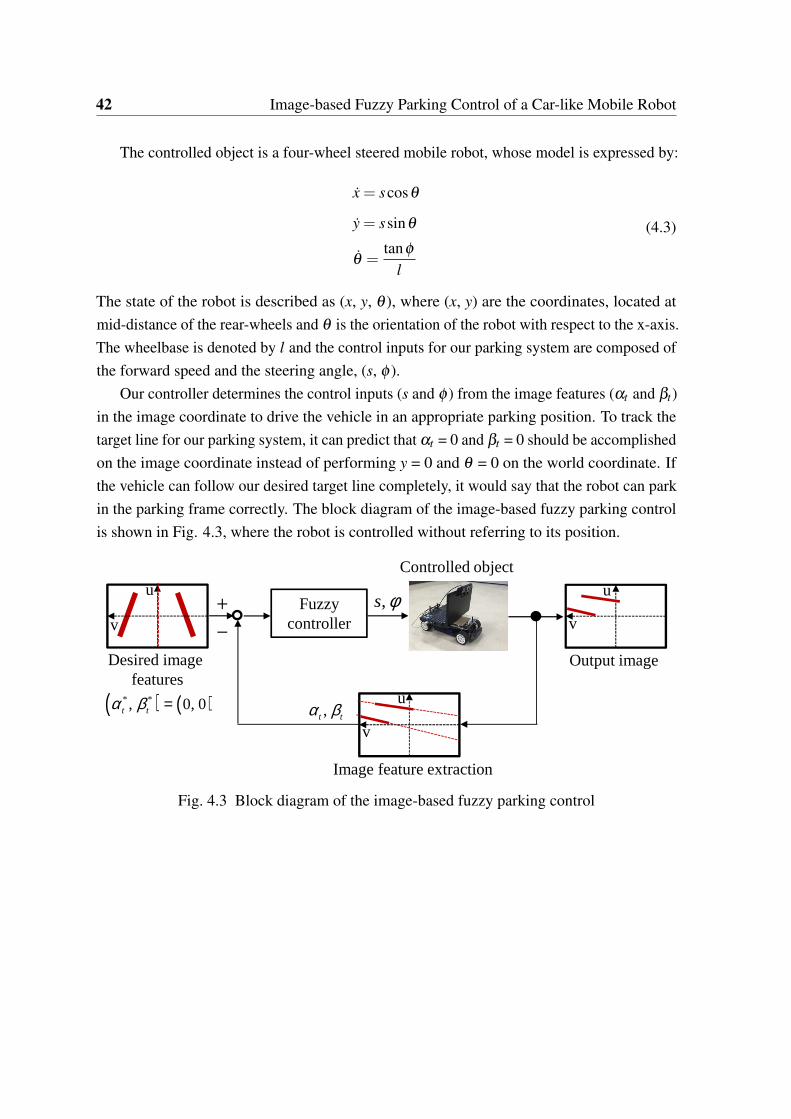
42 Image-based Fuzzy Parking Control of a Car-like Mobile Robot
The controlled object is a four-wheel steered mobile robot, whose model is expressed by:
x = scosθ
y = ssinθ
θ =tanφ
l
(4.3)
The state of the robot is described as (x, y, θ ), where (x, y) are the coordinates, located atmid-distance of the rear-wheels and θ is the orientation of the robot with respect to the x-axis.The wheelbase is denoted by l and the control inputs for our parking system are composed ofthe forward speed and the steering angle, (s, φ ).
Our controller determines the control inputs (s and φ ) from the image features (αt and βt)in the image coordinate to drive the vehicle in an appropriate parking position. To track thetarget line for our parking system, it can predict that αt = 0 and βt = 0 should be accomplishedon the image coordinate instead of performing y = 0 and θ = 0 on the world coordinate. Ifthe vehicle can follow our desired target line completely, it would say that the robot can parkin the parking frame correctly. The block diagram of the image-based fuzzy parking controlis shown in Fig. 4.3, where the robot is controlled without referring to its position.
,s φ�
�
,t tα β( ) ( )* *, 0, 0t tα β =
Image feature extraction
Desired imagefeatures
Fuzzy controller
u
v
u
v
u
v
Output image
Controlled object
Fig. 4.3 Block diagram of the image-based fuzzy parking control
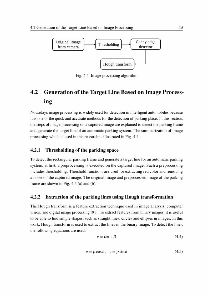
4.2 Generation of the Target Line Based on Image Processing 43
�
Original image from camera
Thresholding
Hough transform
Canny edge detector
Fig. 4.4 Image processing algorithm
4.2 Generation of the Target Line Based on Image Process-ing
Nowadays image processing is widely used for detection in intelligent automobiles becauseit is one of the quick and accurate methods for the detection of parking place. In this section,the steps of image processing on a captured image are explained to detect the parking frameand generate the target line of an automatic parking system. The summarization of imageprocessing which is used in this research is illustrated in Fig. 4.4.
4.2.1 Thresholding of the parking space
To detect the rectangular parking frame and generate a target line for an automatic parkingsystem, at first, a preprocessing is executed on the captured image. Such a preprocessingincludes thresholding. Threshold functions are used for extracting red color and removinga noise on the captured image. The original image and preprocessed image of the parkingframe are shown in Fig. 4.5 (a) and (b).
4.2.2 Extraction of the parking lines using Hough transformation
The Hough transform is a feature extraction technique used in image analysis, computervision, and digital image processing [91]. To extract features from binary images, it is usefulto be able to find simple shapes, such as straight lines, circles and ellipses in images. In thiswork, Hough transform is used to extract the lines in the binary image. To detect the lines,the following equations are used:
v = αu+β (4.4)
u = ρ cosδ , v = ρ sinδ (4.5)
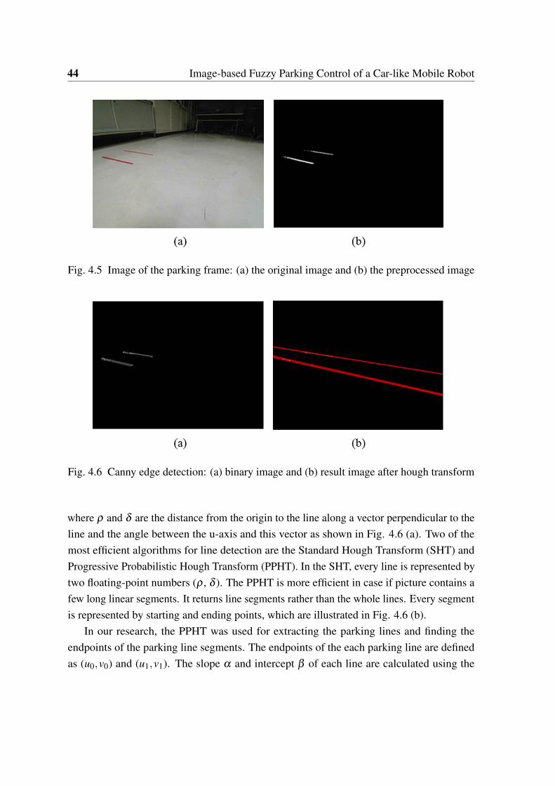
44 Image-based Fuzzy Parking Control of a Car-like Mobile Robot
Fig. 4.5 Image of the parking frame: (a) the original image and (b) the preprocessed image
Fig. 4.6 Canny edge detection: (a) binary image and (b) result image after hough transform
where ρ and δ are the distance from the origin to the line along a vector perpendicular to theline and the angle between the u-axis and this vector as shown in Fig. 4.6 (a). Two of themost efficient algorithms for line detection are the Standard Hough Transform (SHT) andProgressive Probabilistic Hough Transform (PPHT). In the SHT, every line is represented bytwo floating-point numbers (ρ , δ ). The PPHT is more efficient in case if picture contains afew long linear segments. It returns line segments rather than the whole lines. Every segmentis represented by starting and ending points, which are illustrated in Fig. 4.6 (b).
In our research, the PPHT was used for extracting the parking lines and finding theendpoints of the parking line segments. The endpoints of the each parking line are definedas (u0,v0) and (u1,v1). The slope α and intercept β of each line are calculated using the
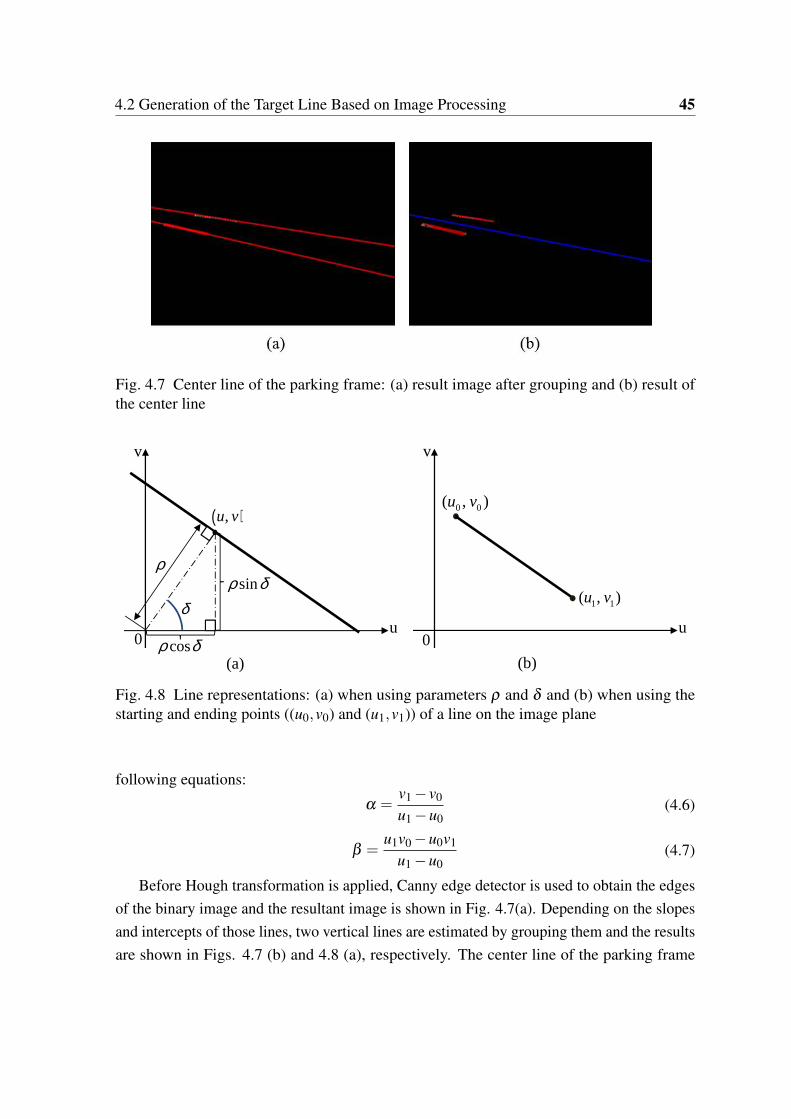
4.2 Generation of the Target Line Based on Image Processing 45
Fig. 4.7 Center line of the parking frame: (a) result image after grouping and (b) result ofthe center line
δ
cosρ δ
sinρ δ
( ),u v
v
u
ρ
0
�
(a)
v
u0
0 0( , )u v
1 1( , )u v
(b)
Fig. 4.8 Line representations: (a) when using parameters ρ and δ and (b) when using thestarting and ending points ((u0,v0) and (u1,v1)) of a line on the image plane
following equations:
α =v1 − v0
u1 −u0(4.6)
β =u1v0 −u0v1
u1 −u0(4.7)
Before Hough transformation is applied, Canny edge detector is used to obtain the edgesof the binary image and the resultant image is shown in Fig. 4.7(a). Depending on the slopesand intercepts of those lines, two vertical lines are estimated by grouping them and the resultsare shown in Figs. 4.7 (b) and 4.8 (a), respectively. The center line of the parking frame
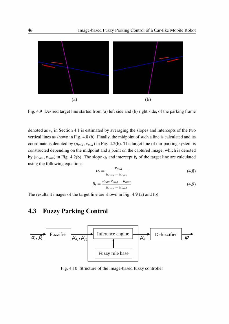
46 Image-based Fuzzy Parking Control of a Car-like Mobile Robot
Fig. 4.9 Desired target line started from (a) left side and (b) right side, of the parking frame
denoted as vc in Section 4.1 is estimated by averaging the slopes and intercepts of the twovertical lines as shown in Fig. 4.8 (b). Finally, the midpoint of such a line is calculated and itscoordinate is denoted by (umid , vmid) in Fig. 4.2(b). The target line of our parking system isconstructed depending on the midpoint and a point on the captured image, which is denotedby (ucam, vcam) in Fig. 4.2(b). The slope αt and intercept βt of the target line are calculatedusing the following equations:
αt =−vmid
ucam −ucam(4.8)
βt =ucamvmid −umid
ucam −umid(4.9)
The resultant images of the target line are shown in Fig. 4.9 (a) and (b).
4.3 Fuzzy Parking Control
�
Inference engine
Fuzzy rule base
Fuzzifier Defuzzifier,t tα βµ µ φµ φ,t tα β
Fig. 4.10 Structure of the image-based fuzzy controller
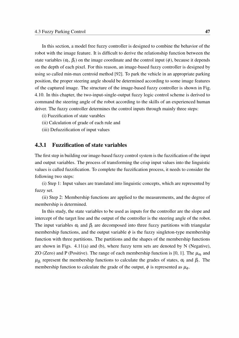
4.3 Fuzzy Parking Control 47
In this section, a model free fuzzy controller is designed to combine the behavior of therobot with the image feature. It is difficult to derive the relationship function between thestate variables (αt , βt) on the image coordinate and the control input (φ ), because it dependson the depth of each pixel. For this reason, an image-based fuzzy controller is designed byusing so called min-max centroid method [92]. To park the vehicle in an appropriate parkingposition, the proper steering angle should be determined according to some image featuresof the captured image. The structure of the image-based fuzzy controller is shown in Fig.4.10. In this chapter, the two-input-single-output fuzzy logic control scheme is derived tocommand the steering angle of the robot according to the skills of an experienced humandriver. The fuzzy controller determines the control inputs through mainly three steps:
(i) Fuzzification of state varables(ii) Calculation of grade of each rule and(iii) Defuzzification of input values
4.3.1 Fuzzification of state variables
The first step in building our image-based fuzzy control system is the fuzzification of the inputand output variables. The process of transforming the crisp input values into the linguisticvalues is called fuzzification. To complete the fuzzification process, it needs to consider thefollowing two steps:
(i) Step 1: Input values are translated into linguistic concepts, which are represented byfuzzy set.
(ii) Step 2: Membership functions are applied to the measurements, and the degree ofmembership is determined.
In this study, the state variables to be used as inputs for the controller are the slope andintercept of the target line and the output of the controller is the steering angle of the robot.The input variables αt and βt are decomposed into three fuzzy partitions with triangularmembership functions, and the output variable φ is the fuzzy singleton-type membershipfunction with three partitions. The partitions and the shapes of the membership functionsare shown in Figs. 4.11(a) and (b), where fuzzy term sets are denoted by N (Negative),ZO (Zero) and P (Positive). The range of each membership function is [0, 1]. The µαt andµβt represent the membership functions to calculate the grades of states, αt and βt . Themembership function to calculate the grade of the output, φ is represented as µφ .
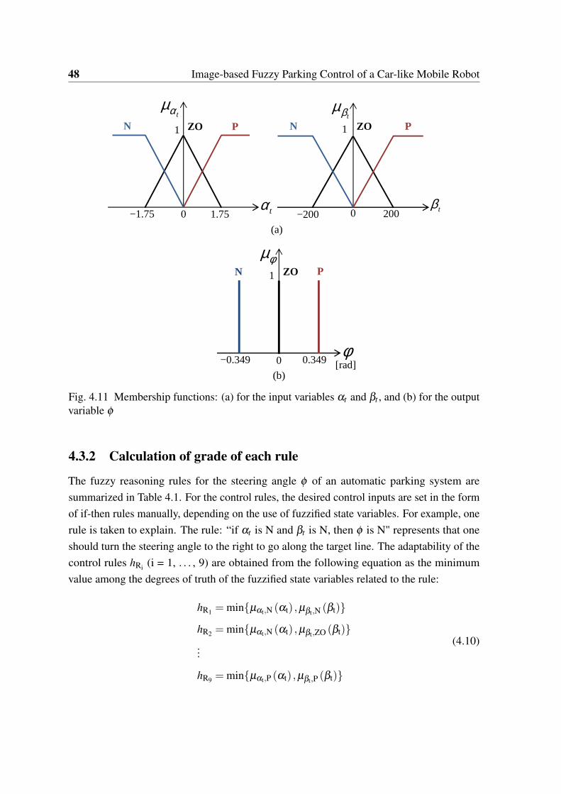
48 Image-based Fuzzy Parking Control of a Car-like Mobile Robot
�
0
N ZO P
tβ
1
0
N ZO P1
φ[rad]
1
0
ZO P
tα
Ntαµ
tβµ
φµ
−1.75 1.75 −200
−0.349
200
0.349
(a)
(b)
Fig. 4.11 Membership functions: (a) for the input variables αt and βt , and (b) for the outputvariable φ
4.3.2 Calculation of grade of each rule
The fuzzy reasoning rules for the steering angle φ of an automatic parking system aresummarized in Table 4.1. For the control rules, the desired control inputs are set in the formof if-then rules manually, depending on the use of fuzzified state variables. For example, onerule is taken to explain. The rule: “if αt is N and βt is N, then φ is N" represents that oneshould turn the steering angle to the right to go along the target line. The adaptability of thecontrol rules hRi (i = 1, . . . , 9) are obtained from the following equation as the minimumvalue among the degrees of truth of the fuzzified state variables related to the rule:
hR1 = min{µαt,N (αt) ,µβt,N (βt)}
hR2 = min{µαt,N (αt) ,µβt,ZO (βt)}...
hR9 = min{µαt,P (αt) ,µβt,P (βt)}
(4.10)
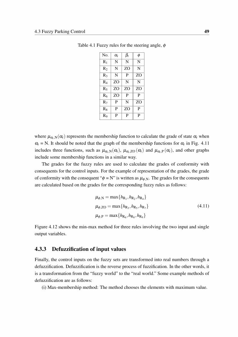
4.3 Fuzzy Parking Control 49
Table 4.1 Fuzzy rules for the steering angle, φ
No. αt βt φ
R1 N N N
R2 N ZO N
R3 N P ZO
R4 ZO N N
R5 ZO ZO ZO
R6 ZO P P
R7 P N ZO
R8 P ZO P
R9 P P P
where µαt ,N(αt) represents the membership function to calculate the grade of state αt whenαt = N. It should be noted that the graph of the membership functions for αt in Fig. 4.11includes three functions, such as µαt ,N(αt), µαt ,ZO (αt) and µαt ,P (αt), and other graphsinclude some membership functions in a similar way.
The grades for the fuzzy rules are used to calculate the grades of conformity withconsequents for the control inputs. For the example of representation of the grades, the gradeof conformity with the consequent “φ = N” is written as µφ ,N. The grades for the consequentsare calculated based on the grades for the corresponding fuzzy rules as follows:
µφ ,N = max{hR1,hR2,hR4}
µφ ,ZO = max{hR3 ,hR5,hR7}
µφ ,P = max{hR6,hR8,hR9}
(4.11)
Figure 4.12 shows the min-max method for three rules involving the two input and singleoutput variables.
4.3.3 Defuzzification of input values
Finally, the control inputs on the fuzzy sets are transformed into real numbers through adefuzzification. Defuzzification is the reverse process of fuzzification. In the other words, itis a transformation from the “fuzzy world” to the “real world.” Some example methods ofdefuzzification are as follows:
(i) Max-membership method: The method chooses the elements with maximum value.
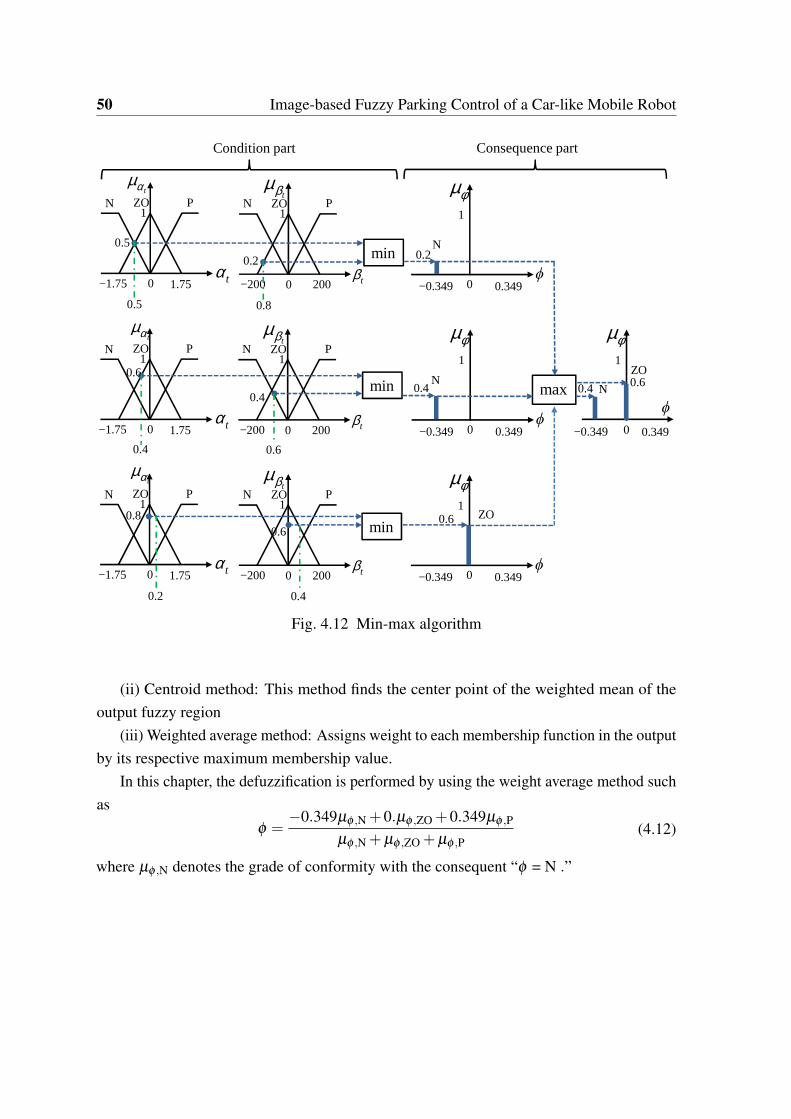
50 Image-based Fuzzy Parking Control of a Car-like Mobile Robot
�
tαµ
0−1.75 1.75 tα
1N ZO P
0−1.75 1.75 tα
1N ZO P
PZON1
−200 2000 tβ
tβµ
PZON1
−200 2000 tβ
tβµ
0.349−0.349ϕ
φµ
0
1
0.349−0.349ϕ
φµ
0
1
0.349−0.349
ϕ
φµ
0
1
tαµ
min
min
max
0−1.75 1.75 tα
1N ZO P PZON
1
−200 2000 tβ
tβµ
0.349−0.349ϕ
φµ
0
1
minN
N
ZO
ZO
N
0.5
0.2 0.2
0.6
0.40.4
0.60.8 0.6
0.60.4
0.5 0.8
0.4 0.6
0.2 0.4
Consequence partCondition part
tαµ
Fig. 4.12 Min-max algorithm
(ii) Centroid method: This method finds the center point of the weighted mean of theoutput fuzzy region
(iii) Weighted average method: Assigns weight to each membership function in the outputby its respective maximum membership value.
In this chapter, the defuzzification is performed by using the weight average method suchas
φ =−0.349µφ ,N +0.µφ ,ZO +0.349µφ ,P
µφ ,N +µφ ,ZO +µφ ,P(4.12)
where µφ ,N denotes the grade of conformity with the consequent “φ = N .”
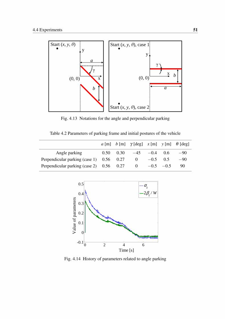
4.4 Experiments 51
�
a
b
γ
y
x(0, 0)
Start (x, y, θ)
γ
b
a
x
y
(0, 0)
Start (x, y, θ), case 1
Start (x, y, θ), case 2
Fig. 4.13 Notations for the angle and perpendicular parking
Table 4.2 Parameters of parking frame and initial postures of the vehicle
a [m] b [m] γ [deg] x [m] y [m] θ [deg]
Angle parking 0.50 0.30 −45 −0.4 0.6 −90Perpendicular parking (case 1) 0.56 0.27 0 −0.5 0.5 −90Perpendicular parking (case 2) 0.56 0.27 0 −0.5 −0.5 90
0 2 4 6-0.1
0
0.1
0.2
0.3
0.4
0.5
Time [s]
Val
ue o
f pa
ram
eter
s
αt
2βt / W
Fig. 4.14 History of parameters related to angle parking
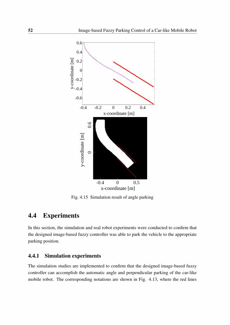
52 Image-based Fuzzy Parking Control of a Car-like Mobile Robot
0
0.
6
x-coordinate [m] -0.4 0 0.5
y-co
ordi
nate
[m
]
-0.4 -0.2 0 0.2 0.4
-0.6
-0.4
-0.2
0
0.2
0.4
0.6
x-coordinate [m]
y-co
ordi
nate
[m
]
Fig. 4.15 Simulation result of angle parking
4.4 Experiments
In this section, the simulation and real robot experiments were conducted to confirm thatthe designed image-based fuzzy controller was able to park the vehicle to the appropriateparking position.
4.4.1 Simulation experiments
The simulation studies are implemented to confirm that the designed image-based fuzzycontroller can accomplish the automatic angle and perpendicular parking of the car-likemobile robot. The corresponding notations are shown in Fig. 4.13, where the red lines
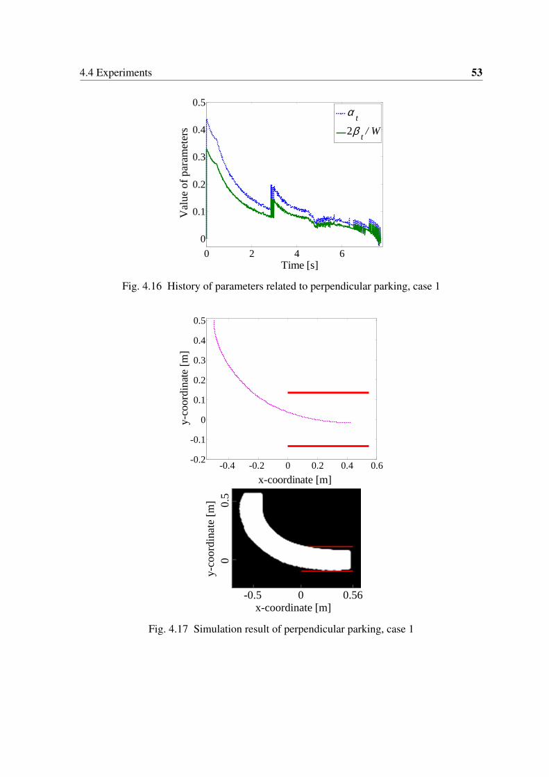
4.4 Experiments 53
0 2 4 6
0
0.1
0.2
0.3
0.4
0.5
Time [s]
Val
ue o
f pa
ram
eter
s
α t
2β t
/ W
Fig. 4.16 History of parameters related to perpendicular parking, case 1
-0.5 0 0.56
0
0.5
x-coordinate [m]
y-co
ordi
nate
[m
]
-0.4 -0.2 0 0.2 0.4 0.6-0.2
-0.1
0
0.1
0.2
0.3
0.4
0.5
x-coordinate [m]
y-co
ordi
nate
[m
]
Fig. 4.17 Simulation result of perpendicular parking, case 1
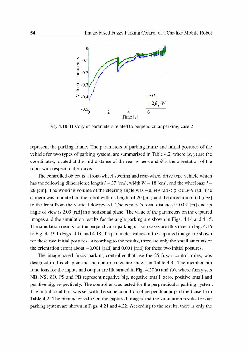
54 Image-based Fuzzy Parking Control of a Car-like Mobile Robot
0 2 4 6-0.5
-0.4
-0.3
-0.2
-0.1
0
Time [s]
Val
ue o
f pa
ram
eter
s
α t
2β t
/W
Fig. 4.18 History of parameters related to perpendicular parking, case 2
represent the parking frame. The parameters of parking frame and initial postures of thevehicle for two types of parking system, are summarized in Table 4.2, where (x, y) are thecoordinates, located at the mid-distance of the rear-wheels and θ is the orientation of therobot with respect to the x-axis.
The controlled object is a front-wheel steering and rear-wheel drive type vehicle whichhas the following dimensions: length l = 37 [cm], width W = 18 [cm], and the wheelbase l =26 [cm]. The working volume of the steering angle was −0.349 rad < φ < 0.349 rad. Thecamera was mounted on the robot with its height of 20 [cm] and the direction of 60 [deg]to the front from the vertical downward. The camera’s focal distance is 0.02 [m] and itsangle of view is 2.09 [rad] in a horizontal plane. The value of the parameters on the capturedimages and the simulation results for the angle parking are shown in Figs. 4.14 and 4.15.The simulation results for the perpendicular parking of both cases are illustrated in Fig. 4.16to Fig. 4.19. In Figs. 4.16 and 4.18, the parameter values of the captured image are shownfor these two initial postures. According to the results, there are only the small amounts ofthe orientation errors about −0.001 [rad] and 0.001 [rad] for these two initial postures.
The image-based fuzzy parking controller that use the 25 fuzzy control rules, wasdesigned in this chapter and the control rules are shown in Table 4.3. The membershipfunctions for the inputs and output are illustrated in Fig. 4.20(a) and (b), where fuzzy setsNB, NS, ZO, PS and PB represent negative big, negative small, zero, positive small andpositive big, respectively. The controller was tested for the perpendicular parking system.The initial condition was set with the same condition of perpendicular parking (case 1) inTable 4.2. The parameter value on the captured images and the simulation results for ourparking system are shown in Figs. 4.21 and 4.22. According to the results, there is only the
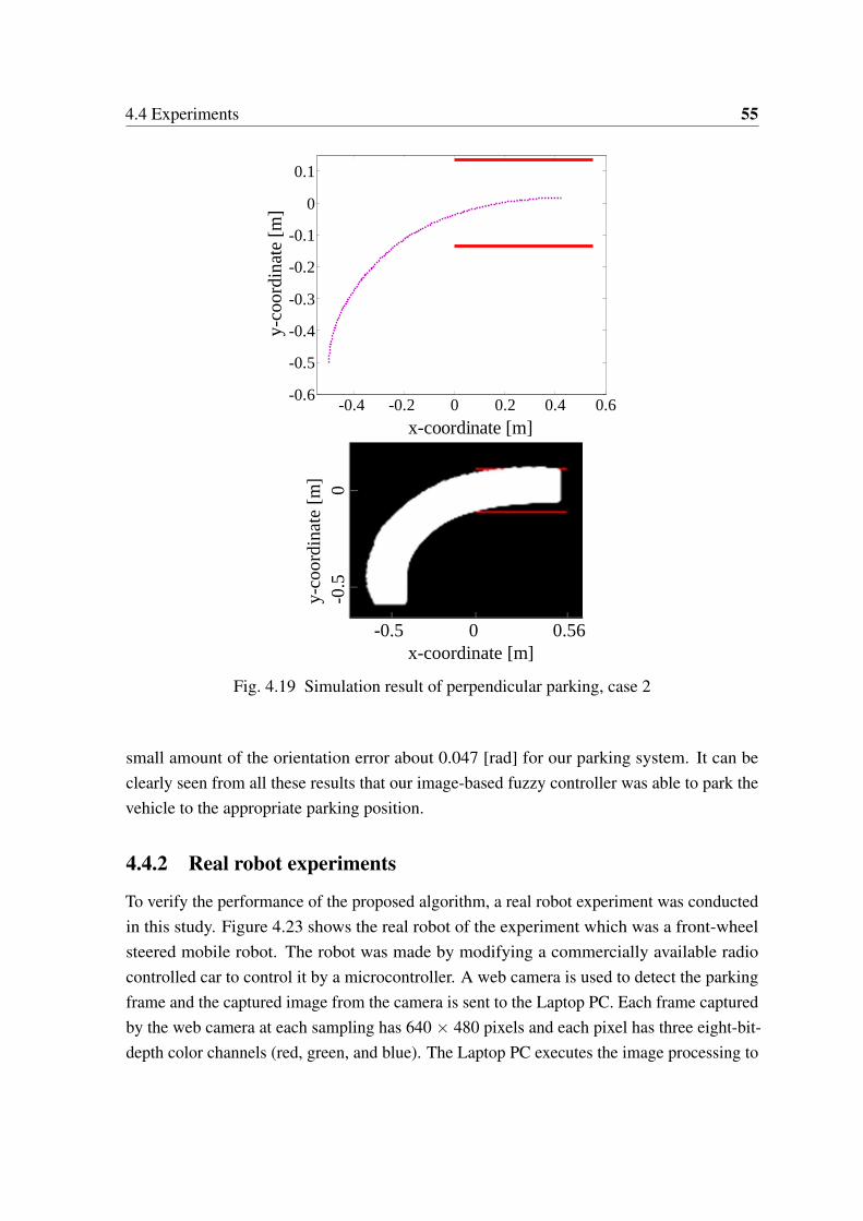
4.4 Experiments 55
-0.5 0 0.56
-0.5
0
x-coordinate [m]
y-co
ordi
nate
[m
]
-0.4 -0.2 0 0.2 0.4 0.6-0.6
-0.5
-0.4
-0.3
-0.2
-0.1
0
0.1
x-coordinate [m]
y-co
ordi
nate
[m
]
Fig. 4.19 Simulation result of perpendicular parking, case 2
small amount of the orientation error about 0.047 [rad] for our parking system. It can beclearly seen from all these results that our image-based fuzzy controller was able to park thevehicle to the appropriate parking position.
4.4.2 Real robot experiments
To verify the performance of the proposed algorithm, a real robot experiment was conductedin this study. Figure 4.23 shows the real robot of the experiment which was a front-wheelsteered mobile robot. The robot was made by modifying a commercially available radiocontrolled car to control it by a microcontroller. A web camera is used to detect the parkingframe and the captured image from the camera is sent to the Laptop PC. Each frame capturedby the web camera at each sampling has 640 × 480 pixels and each pixel has three eight-bit-depth color channels (red, green, and blue). The Laptop PC executes the image processing to
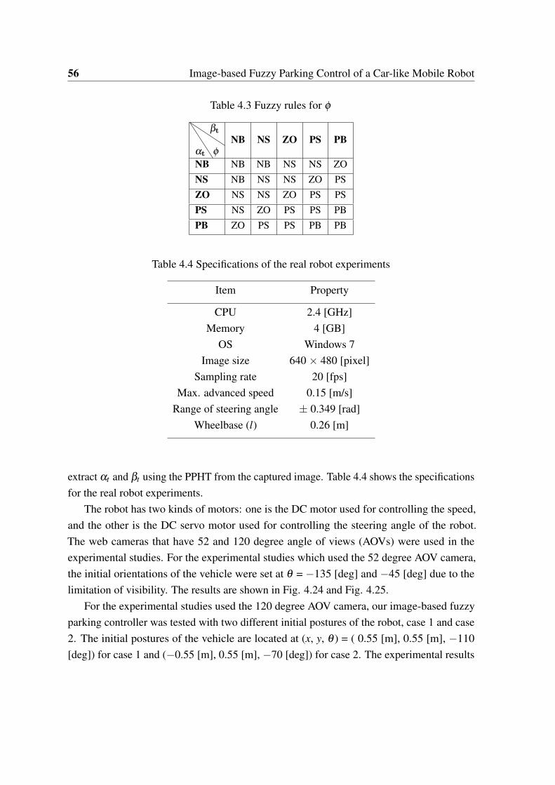
56 Image-based Fuzzy Parking Control of a Car-like Mobile Robot
Table 4.3 Fuzzy rules for φ
αt φ
βt
NB NS ZO PS PB
NB NB NB NS NS ZONS NB NS NS ZO PSZO NS NS ZO PS PSPS NS ZO PS PS PBPB ZO PS PS PB PB
Table 4.4 Specifications of the real robot experiments
Item Property
CPU 2.4 [GHz]Memory 4 [GB]
OS Windows 7Image size 640 × 480 [pixel]
Sampling rate 20 [fps]Max. advanced speed 0.15 [m/s]
Range of steering angle ± 0.349 [rad]Wheelbase (l) 0.26 [m]
extract αt and βt using the PPHT from the captured image. Table 4.4 shows the specificationsfor the real robot experiments.
The robot has two kinds of motors: one is the DC motor used for controlling the speed,and the other is the DC servo motor used for controlling the steering angle of the robot.The web cameras that have 52 and 120 degree angle of views (AOVs) were used in theexperimental studies. For the experimental studies which used the 52 degree AOV camera,the initial orientations of the vehicle were set at θ = −135 [deg] and −45 [deg] due to thelimitation of visibility. The results are shown in Fig. 4.24 and Fig. 4.25.
For the experimental studies used the 120 degree AOV camera, our image-based fuzzyparking controller was tested with two different initial postures of the robot, case 1 and case2. The initial postures of the vehicle are located at (x, y, θ ) = ( 0.55 [m], 0.55 [m], −110[deg]) for case 1 and (−0.55 [m], 0.55 [m], −70 [deg]) for case 2. The experimental results
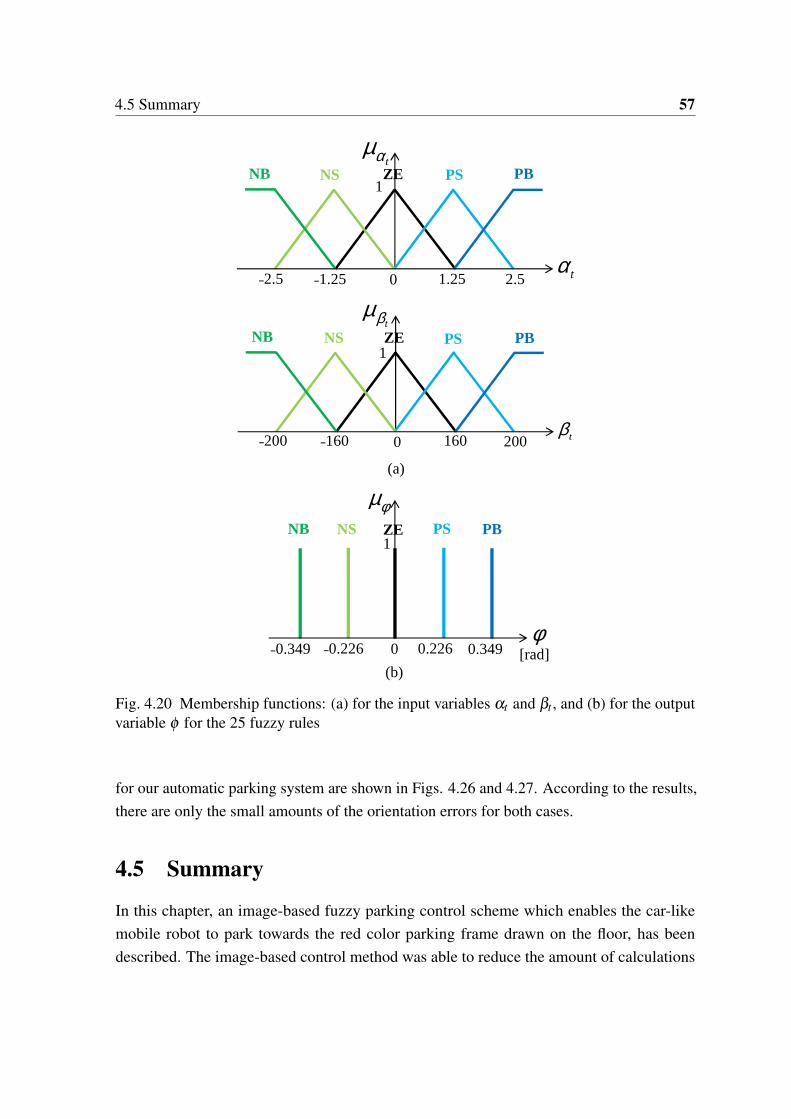
4.5 Summary 57
ZE PS PBNSNB
˗1.25˗2.5 1.25 2.5
1
0
ZE PS PBNSNB1
0 160 200˗160˗200
NB1
NS ZE PS PB
0˗0.349 ˗0.226 0.226 0.349 [rad]
tαµ
tβµ
φµ
tβ
tα
φ
(a)
(b)
Fig. 4.20 Membership functions: (a) for the input variables αt and βt , and (b) for the outputvariable φ for the 25 fuzzy rules
for our automatic parking system are shown in Figs. 4.26 and 4.27. According to the results,there are only the small amounts of the orientation errors for both cases.
4.5 Summary
In this chapter, an image-based fuzzy parking control scheme which enables the car-likemobile robot to park towards the red color parking frame drawn on the floor, has beendescribed. The image-based control method was able to reduce the amount of calculations
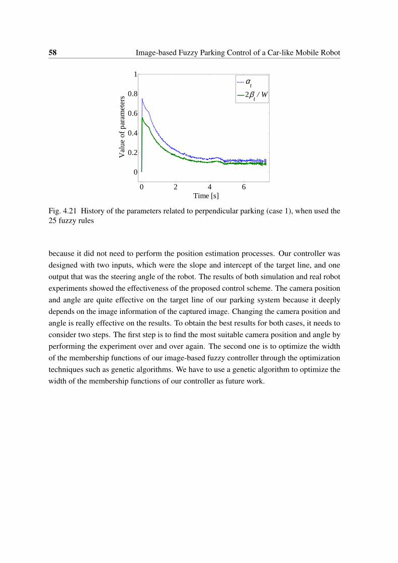
58 Image-based Fuzzy Parking Control of a Car-like Mobile Robot
0 2 4 6
0
0.2
0.4
0.6
0.8
1
Time [s]
Val
ue o
f pa
ram
eter
s
αt
2βt / W
Fig. 4.21 History of the parameters related to perpendicular parking (case 1), when used the25 fuzzy rules
because it did not need to perform the position estimation processes. Our controller wasdesigned with two inputs, which were the slope and intercept of the target line, and oneoutput that was the steering angle of the robot. The results of both simulation and real robotexperiments showed the effectiveness of the proposed control scheme. The camera positionand angle are quite effective on the target line of our parking system because it deeplydepends on the image information of the captured image. Changing the camera position andangle is really effective on the results. To obtain the best results for both cases, it needs toconsider two steps. The first step is to find the most suitable camera position and angle byperforming the experiment over and over again. The second one is to optimize the widthof the membership functions of our image-based fuzzy controller through the optimizationtechniques such as genetic algorithms. We have to use a genetic algorithm to optimize thewidth of the membership functions of our controller as future work.
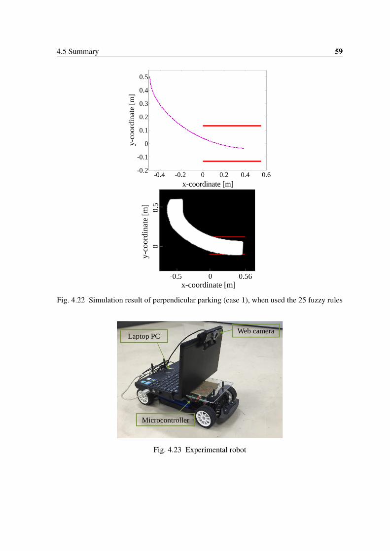
4.5 Summary 59
-0.5 0 0.56
0
0.5
x-coordinate [m]
y-co
ordi
nate
[m
]
-0.4 -0.2 0 0.2 0.4 0.6-0.2
-0.1
0
0.1
0.2
0.3
0.4
0.5
x-coordinate [m]
y-co
ordi
nate
[m
]
Fig. 4.22 Simulation result of perpendicular parking (case 1), when used the 25 fuzzy rules
Web cameraLaptop PC
Microcontroller
Fig. 4.23 Experimental robot
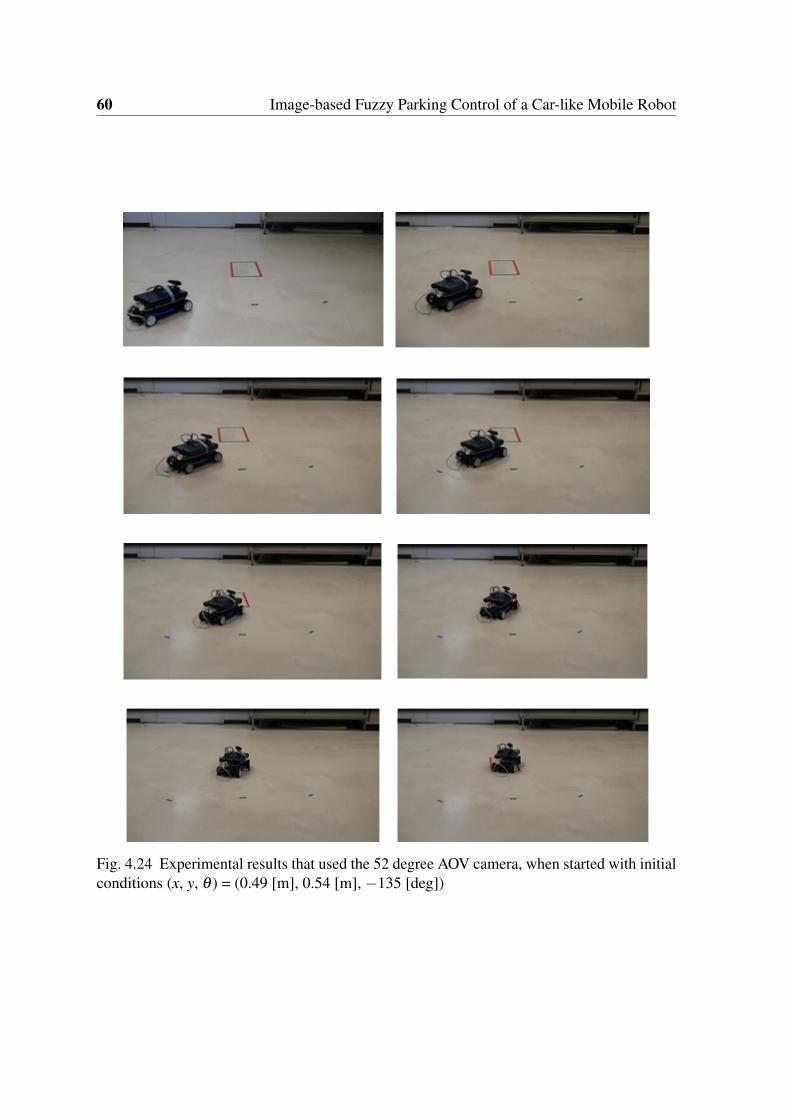
60 Image-based Fuzzy Parking Control of a Car-like Mobile Robot
Fig. 4.24 Experimental results that used the 52 degree AOV camera, when started with initialconditions (x, y, θ ) = (0.49 [m], 0.54 [m], −135 [deg])
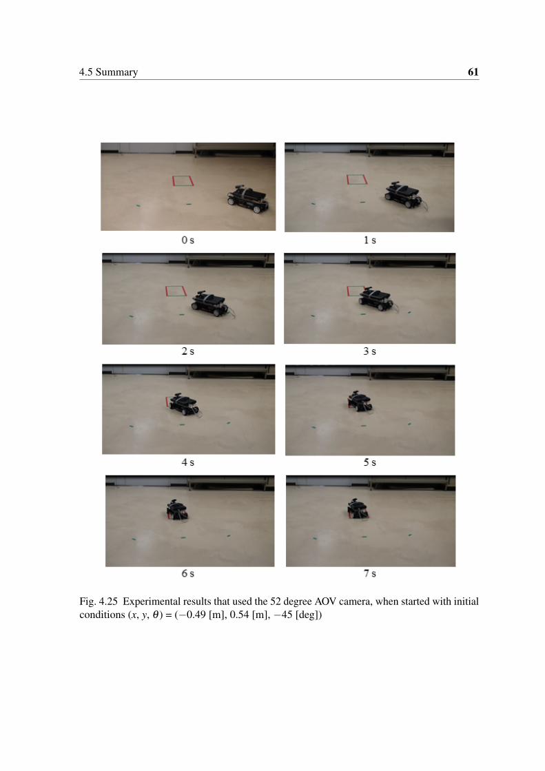
4.5 Summary 61
Fig. 4.25 Experimental results that used the 52 degree AOV camera, when started with initialconditions (x, y, θ ) = (−0.49 [m], 0.54 [m], −45 [deg])
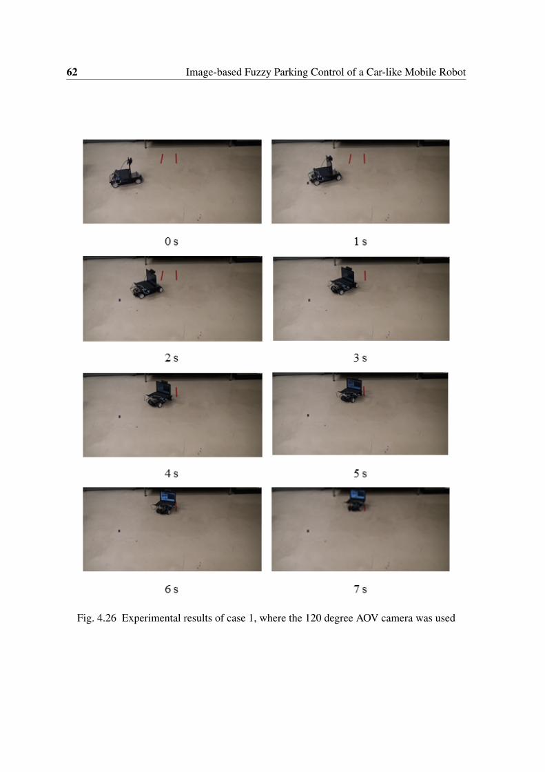
62 Image-based Fuzzy Parking Control of a Car-like Mobile Robot
Fig. 4.26 Experimental results of case 1, where the 120 degree AOV camera was used
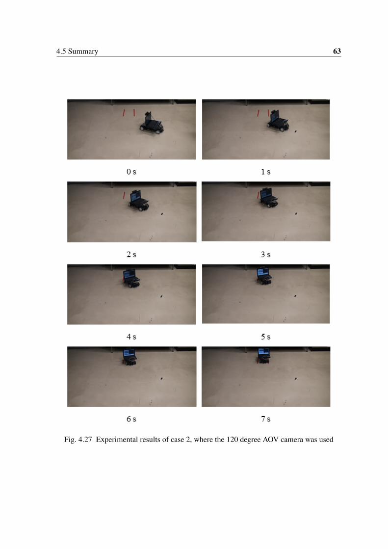
4.5 Summary 63
Fig. 4.27 Experimental results of case 2, where the 120 degree AOV camera was used

Chapter 5
Optimization of an Image-based FuzzyController by a Genetic Algorithm
An automatic parking system of a car-like mobile robot is an important issue in commercialapplications. An image-based fuzzy controller for an automatic parking system of a car-likemobile robot was presented in Chapter 4, where the membership functions were tuned bymanually. However, we know usually that it is not easy to obtain suitable fuzzy membershipfunctions and its rules of a fuzzy controller. For this reason, a genetic algorithm (GA) wasused to optimize the width of the membership functions of our image-based fuzzy controller.
The goal of this chapter is to optimize the parameters of the membership functions, whichwere discussed in previous chapter, by using a GA against the complicated tuning of thecontroller. It is not used to tune the fuzzy reasoning rules because the rules are constructedbased on the skills of the experienced human drivers in advance. The fuzzy rules are verystandard rules and there is not much room to modify them. Adjusting these rules leads toinefficient tuning efforts.
The rest of this chapter is organized as follows. Section 5.1 describes the problem settingand Section 5.2 presents the image-based fuzzy controller to follow the desired trajectory ofour parking system. A method for optimizing the fuzzy controller by GA is developed inSection 5.3. In Section 5.4, some simulation results are given to demonstrate the effectivenessof the proposed method. Section 5.5 summarizes the chapter.
5.1 Problem Setting
An image-based fuzzy parking controller of a car-like mobile robot was developed in ourprevious chapter. In this chapter, the parameters of the membership functions were optimized
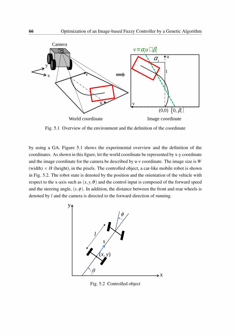
66 Optimization of an Image-based Fuzzy Controller by a Genetic Algorithm
�
World coordinate
u
v(0,0)
t tv uα β= +
tα
1
( )0, tβImage coordinate
v
u
y
x
Camera
Fig. 5.1 Overview of the environment and the definition of the coordinate
by using a GA. Figure 5.1 shows the experimental overview and the definition of thecoordinates. As shown in this figure, let the world coordinate be represented by x-y coordinateand the image coordinate for the camera be described by u-v coordinate. The image size is W(width) × H (height), in the pixels. The controlled object, a car-like mobile robot is shownin Fig. 5.2. The robot state is denoted by the position and the orientation of the vehicle withrespect to the x-axis such as (x,y,θ) and the control input is composed of the forward speedand the steering angle, (s,φ). In addition, the distance between the front and rear wheels isdenoted by l and the camera is directed to the forward direction of running.
x
y
θ
ls
(x��y)
Fig. 5.2 Controlled object
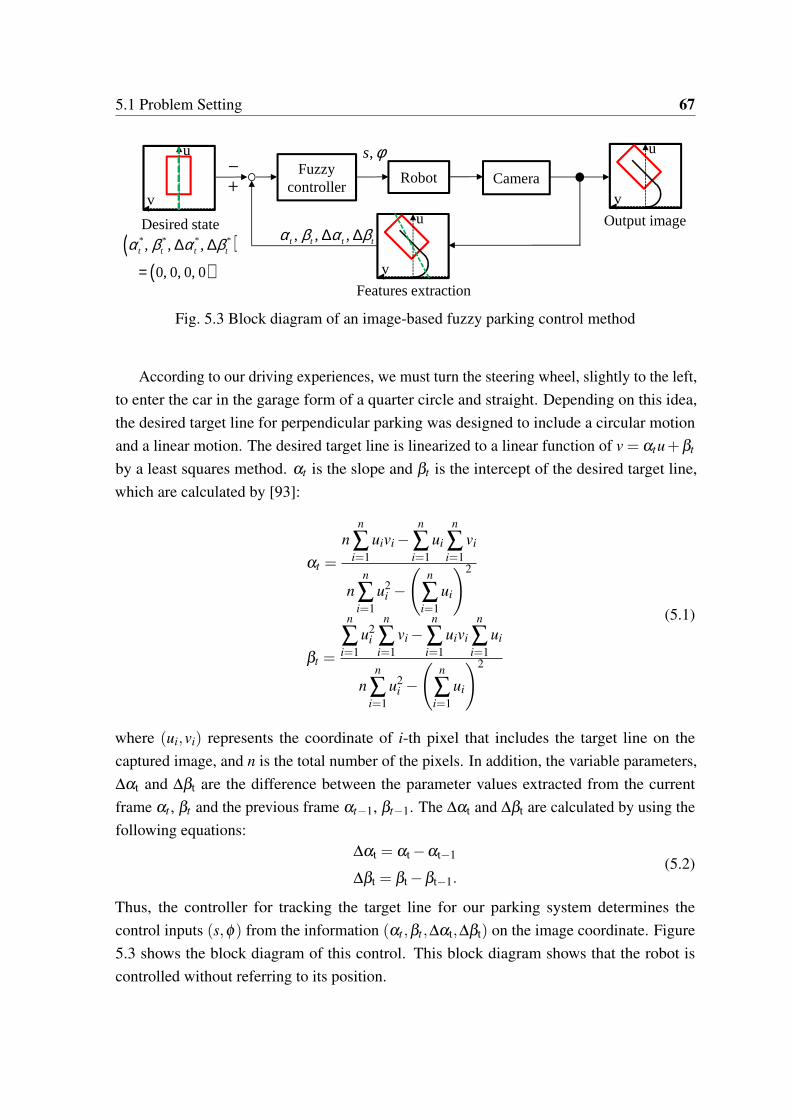
5.1 Problem Setting 67
Fuzzy controller
Robot Camera
Features extraction
�
�
Desired state, , ,t t t tα β α β∆ ∆( )
( )
* * * *, , ,
0, 0, 0, 0
t t t tα β α β∆ ∆
=
,s φu
vOutput image
u
vu
v
Fig. 5.3 Block diagram of an image-based fuzzy parking control method
According to our driving experiences, we must turn the steering wheel, slightly to the left,to enter the car in the garage form of a quarter circle and straight. Depending on this idea,the desired target line for perpendicular parking was designed to include a circular motionand a linear motion. The desired target line is linearized to a linear function of v = αtu+βt
by a least squares method. αt is the slope and βt is the intercept of the desired target line,which are calculated by [93]:
αt =
nn
∑i=1
uivi −n
∑i=1
ui
n
∑i=1
vi
nn
∑i=1
u2i −
(n
∑i=1
ui
)2
βt =
n
∑i=1
u2i
n
∑i=1
vi −n
∑i=1
uivi
n
∑i=1
ui
nn
∑i=1
u2i −
(n
∑i=1
ui
)2
(5.1)
where (ui,vi) represents the coordinate of i-th pixel that includes the target line on thecaptured image, and n is the total number of the pixels. In addition, the variable parameters,∆αt and ∆βt are the difference between the parameter values extracted from the currentframe αt , βt and the previous frame αt−1, βt−1. The ∆αt and ∆βt are calculated by using thefollowing equations:
∆αt = αt −αt−1
∆βt = βt −βt−1.(5.2)
Thus, the controller for tracking the target line for our parking system determines thecontrol inputs (s,φ) from the information (αt ,βt ,∆αt,∆βt) on the image coordinate. Figure5.3 shows the block diagram of this control. This block diagram shows that the robot iscontrolled without referring to its position.
68 Optimization of an Image-based Fuzzy Controller by a Genetic Algorithm
5.2 Image-based Fuzzy Parking Controller
Fuzzy logic control is one of the most successful areas in the application of intelligent control.The application of fuzzy logic does not need much detailed knowledge of the system andutilizes the human (expert) knowledge and intuition instead of the mathematical knowledgeof the system. It includes three components which are fuzzification, fuzzy inference anddefuzzification.
In this work, since the relationship between the parameters, (αt , βt , ∆αt, ∆βt) on theimage coordinate and the control inputs, (s,φ), depends on the depth of each pixel, it may notbe easy to derive the model relation accurately. Therefore, it was decided to use a model-freefuzzy controller. The fuzzified state variables are denoted by (αt , βt , ∆αt, ∆βt) and theirelements are defined by
αt = {N,ZO,P}βt = {N,ZO,P}∆α t = {N,ZO,P}∆β t = {N,ZO,P}
(5.3)
where N, ZO and P are the labels that mean Negative, Zero and Positive, respectively.Figure 5.4 shows the membership functions of each state variable. In the figure, aαt , aβt ,
a∆αt , a∆βt , ass, asb, aφs and aφb are the variables which represent the shape of the membershipfunctions of each state variable. It should be noted that the membership functions for βt
and ∆β t refer to the values of 2βtW and 2∆β t
W which are normalized by the width W of therespective images. The range of each membership function is [0, 1]. The µαt , µβt , µ∆αt , andµ∆βt represent the membership functions to calculate the grades of states, αt , βt , ∆α t , and∆β t . The membership functions to calculate the grade of the control inputs, s and φ , arerepresented as, µs and µφ . Figure 5.5 illustrates the procedure to determine the control inputs,s and φ .
Control rules are considered as 34 types from the four state variables that own three labelsrespectively, which are defined as IF-THEN rules as follows:
R1 : IF αt = N, βt = N, ∆αt = N, ∆βt = N THEN s = s1, φ = φ1
R2 : IF αt = N, βt = N, ∆αt = N, ∆βt = ZO THEN s = s2, φ = φ2
...
R80 : IF αt = P, βt = P, ∆αt = P, ∆βt = ZO THEN s = s80, φ = φ80
R81 : IF αt = P, βt = P, ∆αt = P, ∆βt = P THEN s = s81, φ = φ81
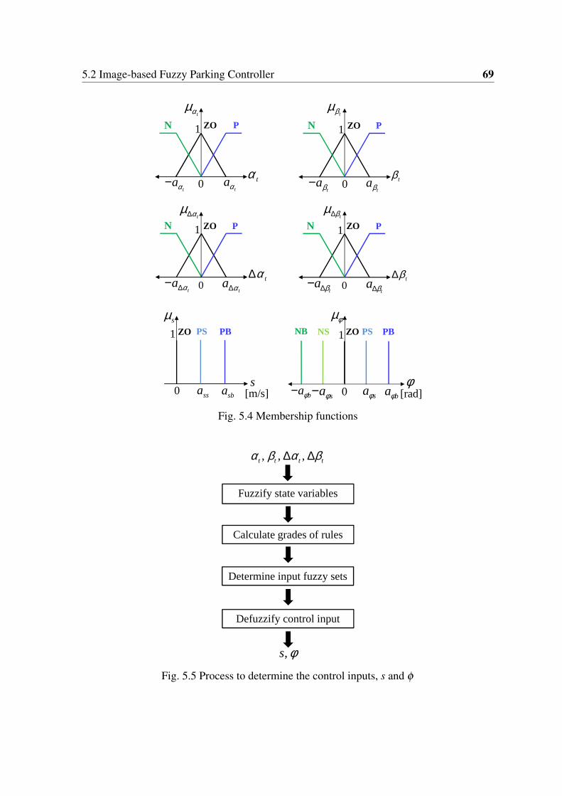
5.2 Image-based Fuzzy Parking Controller 69
1
0
N ZO P
tα
1
0
N ZO P
tβt
aαtaα−
taβt
aβ−
0
ZO PB1
s[m/s]
PS
ssa sba 0
ZO PB1
φ[rad]
PSNSNB
saφ baφsaφ−baφ−
tαµtβµ
1
0
N ZO P
tα∆
1
0
N ZO P
tβ∆t
a α∆ta α∆−
ta β∆t
a β∆−
tαµ∆ tβµ∆
sµ φµ
Fig. 5.4 Membership functions
Fuzzify state variables
Calculate grades of rules
Determine input fuzzy sets
Defuzzify control input
, , ,t t t tα β α β∆ ∆
,s φ
Fig. 5.5 Process to determine the control inputs, s and φ
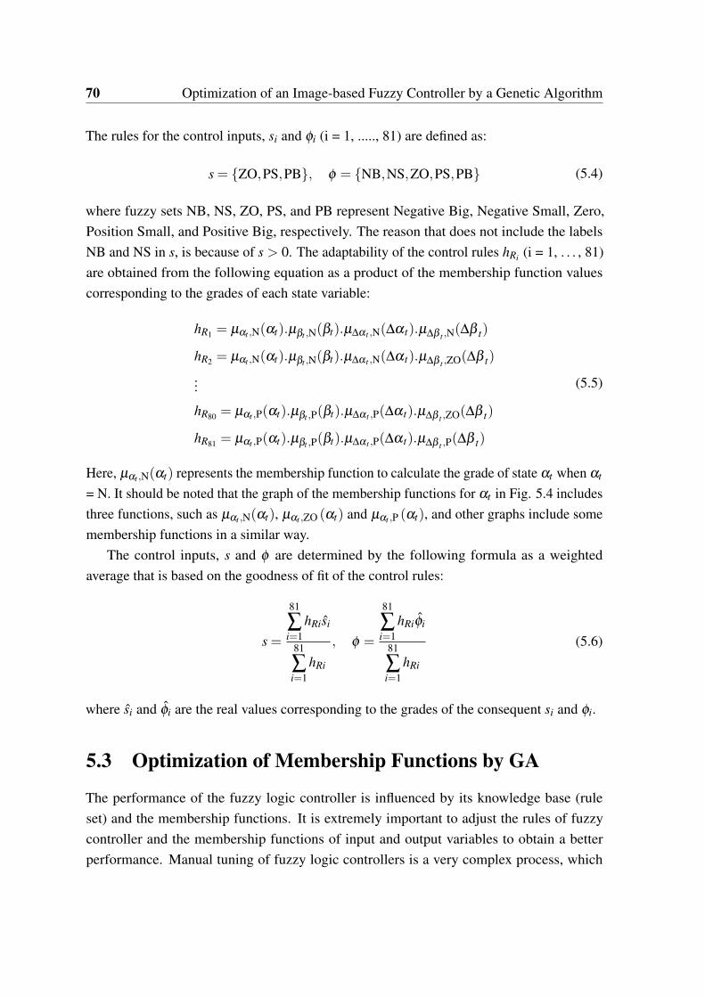
70 Optimization of an Image-based Fuzzy Controller by a Genetic Algorithm
The rules for the control inputs, si and φi (i = 1, ....., 81) are defined as:
s = {ZO,PS,PB}, φ = {NB,NS,ZO,PS,PB} (5.4)
where fuzzy sets NB, NS, ZO, PS, and PB represent Negative Big, Negative Small, Zero,Position Small, and Positive Big, respectively. The reason that does not include the labelsNB and NS in s, is because of s > 0. The adaptability of the control rules hRi (i = 1, . . . , 81)are obtained from the following equation as a product of the membership function valuescorresponding to the grades of each state variable:
hR1 = µαt ,N(αt).µβt ,N(βt).µ∆αt ,N(∆α t).µ∆β t ,N(∆β t)
hR2 = µαt ,N(αt).µβt ,N(βt).µ∆αt ,N(∆α t).µ∆β t ,ZO(∆β t)
...
hR80 = µαt ,P(αt).µβt ,P(βt).µ∆αt ,P(∆α t).µ∆β t ,ZO(∆β t)
hR81 = µαt ,P(αt).µβt ,P(βt).µ∆αt ,P(∆α t).µ∆β t ,P(∆β t)
(5.5)
Here, µαt ,N(αt) represents the membership function to calculate the grade of state αt when αt
= N. It should be noted that the graph of the membership functions for αt in Fig. 5.4 includesthree functions, such as µαt ,N(αt), µαt ,ZO (αt) and µαt ,P (αt), and other graphs include somemembership functions in a similar way.
The control inputs, s and φ are determined by the following formula as a weightedaverage that is based on the goodness of fit of the control rules:
s =
81
∑i=1
hRisi
81
∑i=1
hRi
, φ =
81
∑i=1
hRiφi
81
∑i=1
hRi
(5.6)
where si and φi are the real values corresponding to the grades of the consequent si and φi.
5.3 Optimization of Membership Functions by GA
The performance of the fuzzy logic controller is influenced by its knowledge base (ruleset) and the membership functions. It is extremely important to adjust the rules of fuzzycontroller and the membership functions of input and output variables to obtain a betterperformance. Manual tuning of fuzzy logic controllers is a very complex process, which
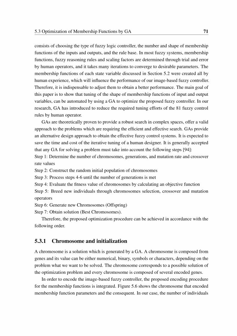
5.3 Optimization of Membership Functions by GA 71
consists of choosing the type of fuzzy logic controller, the number and shape of membershipfunctions of the inputs and outputs, and the rule base. In most fuzzy systems, membershipfunctions, fuzzy reasoning rules and scaling factors are determined through trial and errorby human operators, and it takes many iterations to converge to desirable parameters. Themembership functions of each state variable discussed in Section 5.2 were created all byhuman experience, which will influence the performance of our image-based fuzzy controller.Therefore, it is indispensable to adjust them to obtain a better performance. The main goal ofthis paper is to show that tuning of the shape of membership functions of input and outputvariables, can be automated by using a GA to optimize the proposed fuzzy controller. In ourresearch, GA has introduced to reduce the required tuning efforts of the 81 fuzzy controlrules by human operator.
GAs are theoretically proven to provide a robust search in complex spaces, offer a validapproach to the problems which are requiring the efficient and effective search. GAs providean alternative design approach to obtain the effective fuzzy control systems. It is expected tosave the time and cost of the iterative tuning of a human designer. It is generally acceptedthat any GA for solving a problem must take into account the following steps [94]:Step 1: Determine the number of chromosomes, generations, and mutation rate and crossoverrate valuesStep 2: Construct the random initial population of chromosomesStep 3: Process steps 4-6 until the number of generations is metStep 4: Evaluate the fitness value of chromosomes by calculating an objective functionStep 5: Breed new individuals through chromosomes selection, crossover and mutationoperatorsStep 6: Generate new Chromosomes (Offspring)Step 7: Obtain solution (Best Chromosomes).
Therefore, the proposed optimization procedure can be achieved in accordance with thefollowing order.
5.3.1 Chromosome and initialization
A chromosome is a solution which is generated by a GA. A chromosome is composed fromgenes and its value can be either numerical, binary, symbols or characters, depending on theproblem what we want to be solved. The chromosome corresponds to a possible solution ofthe optimization problem and every chromosome is composed of several encoded genes.
In order to encode the image-based fuzzy controller, the proposed encoding procedurefor the membership functions is integrated. Figure 5.6 shows the chromosome that encodedmembership function parameters and the consequent. In our case, the number of individuals
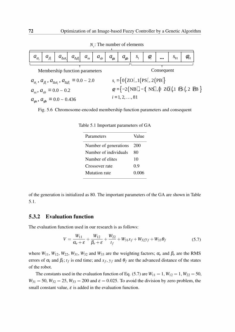
72 Optimization of an Image-based Fuzzy Controller by a Genetic Algorithm
�taα t
aβ ta α∆ t
a β∆ ssa sba saφ baφ 1s 1φ 81s 81φ
cN : The number of elements
ConsequentMembership function parameters
0.0 2.0
0.0 0.2
0.0 0.436
, , ,
,
,
t t t t
ss sb
s b
a a a a
a a
a a
α β α β
φ φ
∆ ∆ =
==
∼
∼
∼
( ) ( ) ( ){ }( ) ( ) ( ) ( ) ( ){ }
0 ZO ,1 PS , 2 PB
2 NB , 1 NS , 0 ZO ,1 PS , 2 PB
1, 2, , 81
i
i
s
i
φ
=
= − −
= …
Fig. 5.6 Chromosome-encoded membership function parameters and consequent
Table 5.1 Important parameters of GA
Parameters Value
Number of generations 200Number of individuals 80Number of elites 10Crossover rate 0.9Mutation rate 0.006
of the generation is initialized as 80. The important parameters of the GA are shown in Table5.1.
5.3.2 Evaluation function
The evaluation function used in our research is as follows:
V =W11
αe + ε+
W12
βe + ε+
W22
t f+W31x f +W32y f +W33θ f (5.7)
where W11, W12, W22, W31, W32 and W33 are the weighting factors; αe and βe are the RMSerrors of αt and βt ; t f is end time; and x f , y f and θ f are the advanced distance of the statesof the robot.
The constants used in the evaluation function of Eq. (5.7) are W11 = 1, W12 = 1, W22 = 50,W31 = 50, W32 = 25, W33 = 200 and ε = 0.025. To avoid the division by zero problem, thesmall constant value, ε is added in the evaluation function.
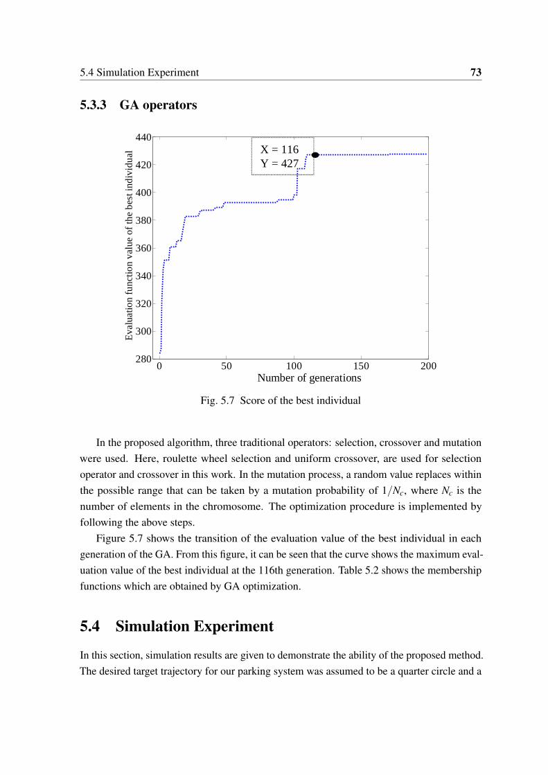
5.4 Simulation Experiment 73
5.3.3 GA operators
0 50 100 150 200280
300
320
340
360
380
400
420
440
Number of generations
Eva
luat
ion
func
tion
valu
e of
the
best
indi
vidu
al X = 116Y = 427
Fig. 5.7 Score of the best individual
In the proposed algorithm, three traditional operators: selection, crossover and mutationwere used. Here, roulette wheel selection and uniform crossover, are used for selectionoperator and crossover in this work. In the mutation process, a random value replaces withinthe possible range that can be taken by a mutation probability of 1/Nc, where Nc is thenumber of elements in the chromosome. The optimization procedure is implemented byfollowing the above steps.
Figure 5.7 shows the transition of the evaluation value of the best individual in eachgeneration of the GA. From this figure, it can be seen that the curve shows the maximum eval-uation value of the best individual at the 116th generation. Table 5.2 shows the membershipfunctions which are obtained by GA optimization.
5.4 Simulation Experiment
In this section, simulation results are given to demonstrate the ability of the proposed method.The desired target trajectory for our parking system was assumed to be a quarter circle and a
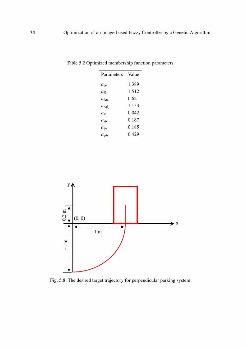
74 Optimization of an Image-based Fuzzy Controller by a Genetic Algorithm
Table 5.2 Optimized membership function parameters
Parameters Value
aαt 1.389aβt 1.512a∆αt 0.62a∆β t
1.153ass 0.042asb 0.187aφs 0.185aφb 0.429
1 m
−1
m
y
x(0, 0)0.
3 m
Fig. 5.8 The desired target trajectory for perpendicular parking system
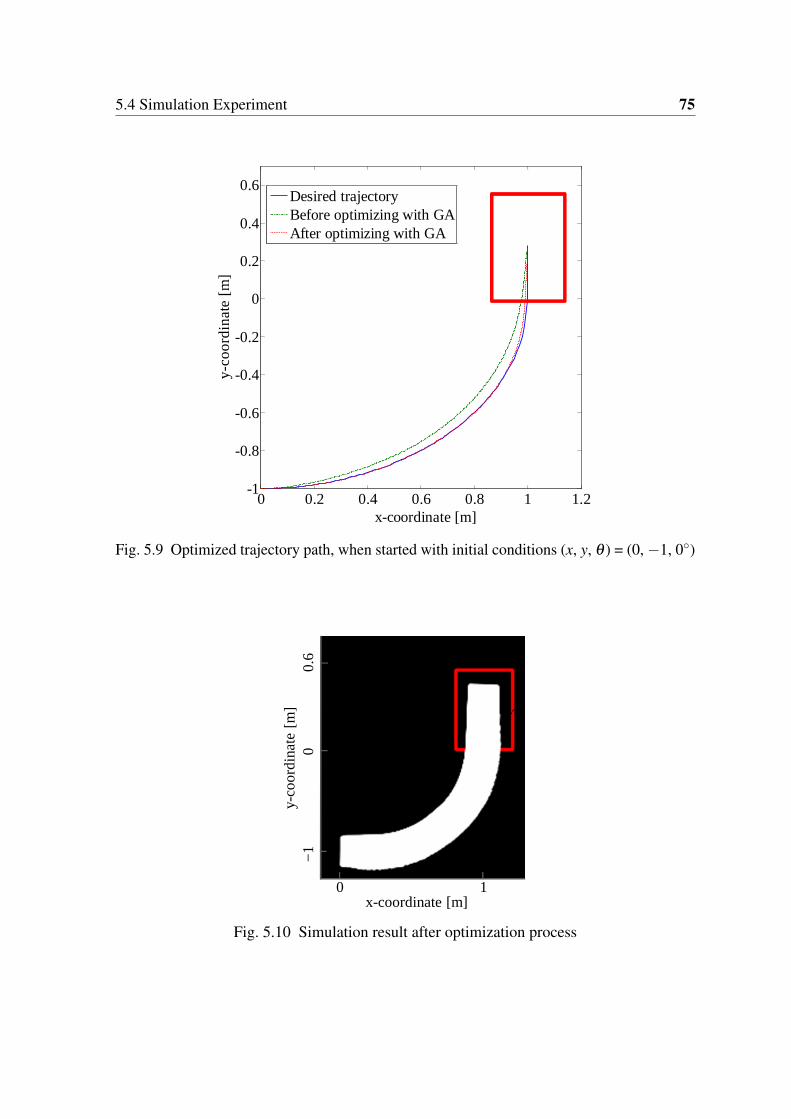
5.4 Simulation Experiment 75
0 0.2 0.4 0.6 0.8 1 1.2-1
-0.8
-0.6
-0.4
-0.2
0
0.2
0.4
0.6
x-coordinate [m]
y-co
ordi
nate
[m
]
Desired trajectoryBefore optimizing with GAAfter optimizing with GA
Fig. 5.9 Optimized trajectory path, when started with initial conditions (x, y, θ ) = (0, −1, 0◦)
x-coordinate [m]
y-co
ord
inat
e [m
]
0 1
−1
0
0.6
Fig. 5.10 Simulation result after optimization process
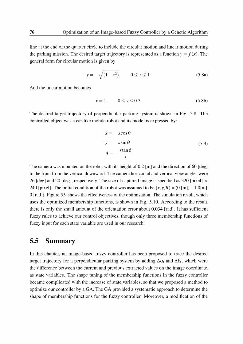
76 Optimization of an Image-based Fuzzy Controller by a Genetic Algorithm
line at the end of the quarter circle to include the circular motion and linear motion duringthe parking mission. The desired target trajectory is represented as a function y = f (x). Thegeneral form for circular motion is given by
y =−√(1− x2), 0 ≤ x ≤ 1. (5.8a)
And the linear motion becomes
x = 1, 0 ≤ y ≤ 0.3. (5.8b)
The desired target trajectory of perpendicular parking system is shown in Fig. 5.8. Thecontrolled object was a car-like mobile robot and its model is expressed by:
x = scosθ
y = ssinθ
θ =s tanφ
l
(5.9)
The camera was mounted on the robot with its height of 0.2 [m] and the direction of 60 [deg]to the front from the vertical downward. The camera horizontal and vertical view angles were26 [deg] and 20 [deg], respectively. The size of captured image is specified as 320 [pixel] ×240 [pixel]. The initial condition of the robot was assumed to be (x,y,θ) = (0 [m], −1.0[m],0 [rad]). Figure 5.9 shows the effectiveness of the optimization. The simulation result, whichuses the optimized membership functions, is shown in Fig. 5.10. According to the result,there is only the small amount of the orientation error about 0.034 [rad]. It has sufficientfuzzy rules to achieve our control objectives, though only three membership functions offuzzy input for each state variable are used in our research.
5.5 Summary
In this chapter, an image-based fuzzy controller has been proposed to trace the desiredtarget trajectory for a perpendicular parking system by adding ∆αt and ∆βt, which werethe difference between the current and previous extracted values on the image coordinate,as state variables. The shape tuning of the membership functions in the fuzzy controllerbecame complicated with the increase of state variables, so that we proposed a method tooptimize our controller by a GA. The GA provided a systematic approach to determine theshape of membership functions for the fuzzy controller. Moreover, a modification of the
5.5 Summary 77
image coordinate, i.e., changing of the v-axis, was able to reduce the y-direction errors. Forexample, even if βt was zero on the old image coordinate in Chapter 4, βt was positive on thenew modified coordinate. Therefore, our controller generated the control inputs to approachthe desired target trajectory more closely. The results confirmed that the proposed methodwas able to trace the desired target trajectory for our parking system.

Chapter 6
Conclusion and Future Work
6.1 Concluding Remarks
In this thesis, the switching and non-switching controllers based on an invariant manifoldtheory, an image-based fuzzy controller, and an optimized image-based fuzzy controller by aGA, have been described to solve the parking problem of a car-like mobile robot.
For stabilizing the car-like mobile robot in the desired posture, Chapter 3 has presentedthe switching and non-switching controllers based on an invariant manifold theory. It wasfound that our invariant manifold approach consists an incomplete manifold under a linearstate feedback controller, which makes all the states tend to the desired position except thevehicle orientation. For this reason, the linear state feedback controller was enhanced byan additional state feedback to make the constructed manifold with the method of Tayebiet al. [7]. It has been proved from the results that the switching controllers converged thevehicle to the desired states when the initial states were θ = 1 radian and φ = 0 . On the otherhand, the non-switching controller was able to make the vehicle to be stable and convergedto the desired states for both parking types.
In the above approach, it was assumed that the robot states can be exactly obtained for thefeedback control purpose. This assumption is usually not satisfied in a real parking systemdue to the uncertainties in the kinematic model and slippage of the wheels on the ground. Forthis reason, an image-based fuzzy controller for an automatic parking system of a car-likemobile robot has been presented in Chapter 4. In this approach, the image informationwhich was acquired from a camera image was used to control a robot without using the robotposition. A model-free fuzzy controller was designed to combine the behavior of the robotwith the image features without estimating the image depth. The results proved that ourimage-based fuzzy controller was able to park the vehicle to the appropriate parking position.
80 Conclusion and Future Work
It is well known that the performance of the fuzzy logic controller is influenced by itsknowledge base and the membership functions. To obtain the best performance of fuzzylogic controller, it is very important to optimize the rules and the widths of the membershipfunctions of input and output variables of fuzzy logic controller. However, the process ofmanually tuning the fuzzy logic controller is a very complex task. Chapter 5 has presentedthe process of optimizing the widths of membership functions of our image-based fuzzyparking controller by using a GA against the complicated tuning of the controller. It wasproved that the tuning of the shape of membership functions of input and output variablescan be automated by using the GA to optimize the proposed image-based fuzzy controller.The simulation results were given to confirm that our optimized image-based fuzzy controllerwas able to trace the desired target trajectory of the perpendicular parking system.
6.2 Future Work
We have to test the GA optimized image-based fuzzy controller on some real robot experi-ments for parking problem as a future work.
In this dissertation, our image-based fuzzy controller was tested only for forward parkingsystem and the backward parking system is left for future study. In the backward parkingsystem, the first task is to find a suitable path from the initial parking position to the switchingpoint, from where it is ensured that the vehicle is able to leave the parking spot.
The image-based fuzzy parking control system described in this thesis did not considerthe avoidance of unforeseen obstacles, but focused on the parking the vehicle in a constrainedparking lot. The parking system, which considers for obstacle environments should beinvestigated in the future study.
References
[1] I. Kolmanovsky and N. H. McClamroch, “Developments in nonholonomic controlproblems,” IEEE Control Systems Magazine, vol. 15, no. 6, pp. 20–36, 1995.
[2] R. W. Brockett, “Asympototic stability and feedback stabilization,” Differential Geo-metric Control Theory, vol. 27, no. 1, pp. 181–191, 1983.
[3] J. B. Pomet, “Explicit design of time-varying stabilizing control laws for a classof controllable systems without drift,” Systems and Control Letter, vol.18, no. 2,pp. 147–158, 1992.
[4] C. Samson, “Control of chained systems application to path following and time-varyingpoint-stabilization of mobile robots,” IEEE Transactions on Automatic Control, vol. 40,no. 1, pp. 64–77, 1995.
[5] A. Astolfi, “Discontinuous control of nonholonomic systems,” System and ControlLetters, vol. 27, no. 1, pp. 37–45, 1996.
[6] A. Tayebi, M. Tadjine, and A. Rachid, "Discontinuous control design for the stabi-lization of nonholonomic systems in chained form using the backstepping approach:Application to mobile robots,” in Proceedings of the 36th IEEE Conference on Deci-sion and Control, 1997, pp. 3089–3090.
[7] A. Tayebi, M. Tadjine, and A. Rachid, “Invariant manifold approach for the stabliza-tion of nonholonomic chained systems: Application to a mobile robot,” NonlinearDynamics, vol. 24, no. 2, pp. 167–181, 2001.
[8] H. Khennouf and C. C. De Wit, “Quasicantinuous exponential stabilizers for nonholo-nomic systems,” in Proceedings of IFAC 13th World Congress, 1996, pp. 49–54.
[9] H. Khennouf and C. Canudas de Wit, “On the construction of stabilizing discontinuouscontrollers for nonholonomic system,” in Proceedings of IFAC Nonlinear ControlSystems Design Symp. (NOLCOS’ 95), 1995, pp. 667–672.
82 References
[10] K. Watanabe, T. Yamamoto, K. Izumi, and S. Maeyama, “Underactuated control fornonholonomic mobile robots by using double integrator model and invariant manifoldtheory,” in Proceedings of 2010 IEEE/RSJ International Conference on IntelligentRobots and Systems (IROS), 2010, pp. 2862–2867.
[11] T. Yamamoto and K. Watanabe, “A switching control method for stabilizing a non-holonomic mobile robot using invariant manifold method,” in Proceedings of SICEAnnual Conference, 2010, pp. 3278–3284.
[12] K. Watanabe, Y. Ueda, and I. Nagai, “Underactuated control for a fire truck-type mo-bile robot using an invariant manifold theory,” in Proceedings of the 6th InternationalConference on Soft Computing and Intelligent Systems and the 13th InternationalSymposium on Advances Intelligent Systems (SCIS-ISIS), 2012, pp. 210–215.
[13] K. Watanabe, Y. Ueda, I. Nagai, and S. Maeyama, “Stabilization of a fire truck robotby an invariant manifold theory,” Procedia Engineering, vol. 41, pp. 1095–1104, 2012.
[14] K. Izumi and K. Watanabe, “Switching manifold control for an extended nonholonomicdouble integrator,” in Proceedings of International Conference on Control Automationand Systems (ICCAS), 2010, pp. 27–30.
[15] M. Reyhanoglu, “On the stabilization of a class of nonholonomic systems using invari-ant manifold technique,” in Proceedings of the 34th IEEE Conference On Decisionand Control, 1995, pp. 2125–2126.
[16] S. Lee, M. Kim, Y. Youm, and W. Chung, “Control of a car-like mobile robot forparking problem,” in Proceedings of IEEE International Conference Robotics andAutomation, 1990, pp. 1–6.
[17] N. Marchand and M. Alamir, “Discontinuous exponential stabilization of chainedform systems,” Automatica, vol. 39, no. 2, pp. 343–348, 2003.
[18] A. M. Bloch, M. Reyhanoglu, and N. H. McClamroch, “Control and stabilization ofnonholonomic dynamic systems,” IEEE Transactions on Automatic Control, vol. 37,no. 11, pp. 1746–1757, 1992.
[19] Y. P. Tian and S. Li, “Exponential stabilization of nonholonomic dynamic systems bysmooth time-varying control,” Automatica, vol. 38, no. 7, pp. 1139–1146, 2002.
[20] Y. Hu, S. S. Ge, and C. Y. Su, “Stabilization of uncertain nonholonomic systems viatime-varying sliding mode control,” IEEE Transactions on Automatic Control, vol. 49,no. 5, pp. 757–763, 2004.
References 83
[21] E. Malis, “Survey of vision-based control,” ENSIETA European Naval Ship DesignShort Course, Brest, France, 2002.
[22] D. Tsakiris, C. Samson, and P. Rives, “Vision-based time-varying stabilization ofa mobile manipulator,” in Proceedings of 6th International Conference on Control,Automation, Robotics and Vision (ICARV), 1996.
[23] I. Horswill, “Polly: A vision-based artificial agent,” in Proceedings of the 11thNational Conference on Artificial Intelligence (AAAI-93), 1993, pp. 824–829.
[24] A. K. Das, R. Fierro, V. Kumar, B. Southall, J. Spletzer, and C. J. Taylor, “Real-time vision-based control of a nonholonomic mobile robot,” in Proceedings of IEEEInternational Conference on Robotics and Automation, 2001, pp.1714–1719.
[25] R. Carelli, C. M. Soria, and B. Morales, “Vision-based tracking control for mobilerobots,” in Proceedings of 12th International Conference on Advanced Robotics(ICAR), 2005, pp. 148–152.
[26] N. R. Gans and S. A. Hutchinson, “A stable vision-based control scheme for non-holonomic vehicles to keep a landmark in the field of view,” in Proceedings of IEEEInternational Conference on Robotics and Automation, 2007, pp. 2196–2201.
[27] A. Cherubini, F. Chaumette, and G. Oriolo, “A position-based visual servoing schemefor following paths with nonholonomic robots,” in Proceedings of IEEE/RSJ Interna-tional Conference on Intelligent Robots and Systems (IROS), 2008, pp. 1648–1654.
[28] Y. Masutani, M. Mikawa, N. Maru, and F. Miyazaki, “Visual servoing for non-holonomic mobile robots,” in Proceedings of the IEEE/RSJ/GI International Confer-ence on Intelligent Robots and Systems, 1994, pp. 1133–1140.
[29] R. Pissard-Gibollet and P. Rives, “Applying visual servoing techniques to controla mobile hand-eye system,” in Proceedings of IEEE International Conference onRobotics and Automation, 1995, pp. 166–171.
[30] K. Hashimoto and T. Noritsugu, “Visual servoing of nonholonomic cart,” in Proceed-ings of IEEE International Conference on Robotics and Automation, vol. 2, 1997,pp. 1719–1724.
[31] N. R. Gans and S. A. Hutchinson, “A stable vision-based control scheme for non-holonomic vehicles to keep a landmark in the field of view,” in Proceedings of IEEEInternational Conference on Robotics and Automation, 2007, pp. 2196–2201.
84 References
[32] B. Thuilot, P. Martinet, L. Cordesses, and J. Gallice, “Position based visual servoing:Keeping the object in the field of vision,” in Proceedings of the IEEE InternationalConference on Robotics and Automation, vol. 2, 2002, pp. 1624–1629.
[33] I. J. Ha, D. H. Park, and J. H. Kwon, “A novel position-based visual servoing ap-proach for robust global stability with feature points kept within the field-of-view,” inProceedings of 11th International Conference on Control, Automation, Robotics andVision, 2010, pp. 1458–1465.
[34] B. Espiau, “Effect of camera calibration errors on visual servoing in robotics,” inProceedings of the 3rd International Symposium on Experimental Robotics III, 1994,pp. 182–192.
[35] S. Hutchinson, G. D. Hager, and P. I. Corke, “A tutorial on visual servo control,” IEEETransactions on Robotics and Automation, vol. 12, no. 5, pp. 651–670, 1996.
[36] F. Conticelli, B. Allotta, and P. K. Khosla, “Image-based visual servoing of non-holonomic mobile robots,” in Proceedings of the 38th IEEE Conference on DecisionControl, 1999, pp. 3496–3501.
[37] H. Y. Wang, S. Itani, T. Fukao, and N. Adachi, “Image-based visual adaptive trackingcontrol of nonholonomic mobile robots,” in Proceedings of IEEE/RSJ InternationalConference on Intelligent Robots and Systems, 2001, pp. 1–6.
[38] G. L. Mariottini, G. Oriolo, and D. Prattichizzo, “Image-based visual servoing for non-holonomic mobile robots using epipolar geometry,” IEEE Transactions on Robotics,vol. 23, no. 1, pp. 87–100, 2007.
[39] G. L. Mariottini, D. Prattichizzo, and G. Oriolo, “Image-based visual servoing fornonholonomic mobile robots with central catadioptric camera,” in Proceedings ofIEEE International Conference on Robotics and Automation, 2006, pp. 538–544.
[40] R. Rao, V. Kumar, and C. Taylor, “Visual servoing of a UGV from a UAV using differ-ential flatness,” in Proceedings of IEEE/RSJ International Conference on IntelligentRobots and Systems, 2003, pp. 743–748.
[41] Y. Ma, J. Kosecka, and S. S. Sastry, “Vision-guided navigation for a nonholonomicmobile robot,” IEEE Transactions on Robotics and Automation, vol. 15, no. 3,pp. 521–536, 1999.
References 85
[42] T. Kato, K. Watanabe, and S. Maeyama, “Image-based fuzzy trajectory trackingcontrol for four-wheel steered mobile robots,” Artificial Life and Robotics, vol. 17,no. 1, pp. 130–135, 2012.
[43] K. Watanabe, T. Kato, and S. Maeyama, “Obstacle avoidance for mobile robotsusing an image-based fuzzy controller,” in Proceedings of IECON 2013-39th AnnualConference of the IEEE Industrial Electronics Society, 2013, pp. 6392–6397.
[44] G. M. Chen, P. Z. Lin, W. Y. Wang, T. T. Lee, and C. H. Wang, “Image-based fuzzycontrol system,” Electronics Letters, vol. 44, no. 7, pp. 461–462, 2008.
[45] E. Malis, F. Chaumette, and S. Boudet, “2½D visual servoing,” IEEE Transactions onRobotics and Automation, vol. 15, no. 2, pp. 238–250, 1999.
[46] P. Murrieri, D. Fontanelli, and A. Bicchi, “A hybrid-control approach to the park-ing problem of a wheeled vehicle using limited view-angle visual feedback,” TheInternational Journal of Robotics Research, vol. 23, no. 4-5, pp. 437–448, 2004.
[47] Y. Fang, W. E. Dixon, D. M. Dawson, and P. Chawda, “Homography-based visualservo regulation of mobile robots,” IEEE Transactions on Systems, Man, and Cyber-netics, Part B (Cybernetics), vol. 35, no. 5, pp. 1041–1050, 2005.
[48] C. Colombo, B. Allotta, and P. Dario, “Affine visual servoing: A framework forrelative positioning with a robot,” in Proceedings of IEEE International Conferenceon Robotics and Automation, 1995, pp. 464–471.
[49] P. Questa, E. Grossmann, and G. Sandin, “Camera self orientation and dockingmaneuver using normal flow,” in Proceedings of the SPIE’s 1995 Symposium onOE/Aerospace Sensing and Dual Use Photonics, 1995, pp. 274–283.
[50] A. Cretual and F. Chaumette, “Positionning a camera parallel to a plane using dynamicvisual servoing,” in Proceedings of IEEE International Conference on IntelligentRobots and Systems, vol. 1, 1997, pp. 43–48.
[51] L. A. Zadeh, “Fuzzy sets,” Information Control, vol. 8, no. 3, pp. 338–353, 1965.
[52] S. S. Chang and L. A. Zadeh, “On fuzzy mapping and control,” IEEE Transactions onSystems, Man and Cybernetics, no. 1, pp. 30–34, 1972.
[53] K. Tanaka and M. Sano, “Trajectory stabilization of a model car via fuzzy control,”Fuzzy Sets and Systems, vol. 70, no. 2-3, pp. 155–170, 1995.
86 References
[54] Y. C. Chiou and L. W. Lan, “Genetic fuzzy logic controller: An iterative evolutionalgorithm with new encoding method,” Fuzzy Sets and Systems, vol. 152, no. 3,pp. 617–635, 2005.
[55] A. Homaifar and E. McCormick, “Simultaneous design of membership functions andrule sets for fuzzy controllers using genetic algorithms,” IEEE Transactions on FuzzySystems, vol. 3, no. 2, pp. 129–139, 1995.
[56] L. A. Zadeh, “Fuzzy algorithm,” Information Control, vol. 12, pp. 94–102, 1968.
[57] C. Von Altrock, B. Krause, and H. J. Zimmermann, “Advanced fuzzy logic con-trol technologies in automotive applications,” in Proceedings of IEEE InternationalConference on Fuzzy Systems, 1992, pp. 835–842.
[58] T. Das and I. N. Kar, “Design and implementation of an adaptive fuzzy logic-based con-troller for wheeled mobile robots,” IEEE Transactions on Control Systems Technology,vol. 14, no. 3, pp. 501–510, 2006.
[59] V. M. Peri and D. Simon, “Fuzzy logic controller for an autonomous robot,” inProceedings of NAFIPS 2005-2005 Annual Meeting of the North American FuzzyInformation Processing Society, pp. 337–342, 2005.
[60] M. K. Singh, D. R. Parhi, S. Bhowmik, and S. K. Kashyap, “Intelligent controllerfor mobile robot: Fuzzy logic approach,” in Proceedings of the 12th InternationalConference of International Association for Computer Methods and Advances inGeomechanics (IACMAG), 2008, pp. 1–6.
[61] J. Xu, G. Chen, and M. Xie, “Vision-guided automatic parking for smart car,” inProceedings of IEEE Intelligent Vehicle Symposium, 2000, pp. 725–730.
[62] Y. Zhao and E. G. Collin, “Robust automatic parallel parking in tight spaces via fuzzylogic,” Robotics and Autonomous Systems, vol. 51, no. 2, pp. 111–127, 2005.
[63] T. H. Li and S. J. Chang, “Autonomous fuzzy parking control of a car-like mobilerobot,” IEEE Transactions on Systems, Man, and Cybernetics-Part A: Systems andHumans, vol. 33, no. 4, pp. 451–465, 2003.
[64] T. H. Li, S. J. Chang, and Y. X. Chen, “Implementation of human-like driving skills byautonomous fuzzy behavior control on an FPGA-based car-like mobile robot,” IEEETransactions on Industrial Electronics, vol. 50, no. 5, pp. 867–880, 2003.
References 87
[65] I. Baturonel, F. J. Moreno-Velo, S. Sánchez-Solano, and A. Ollero, “Automatic designof fuzzy controllers for car-like autonomous robots,” IEEE Transacions on FuzzySystems, vol. 12, no. 4, pp. 447–465, 2004.
[66] M. Sugeno, “An experimental study on fuzzy parking control using a model car,”Industrial Applications of Fuzzy Control, pp. 105–124, 1985.
[67] A. Razinkova, H. C. Cho, and H. T. Jeon, “An intelligent auto parking system forvehicles,” International Journal of Fuzzy Logic and Intelligent Systems, vol. 12, no. 3,pp. 226–231, 2012.
[68] F. Gómez-Bravo, F. Cuesta, and A. Ollero, “Parallel and diagonal parking in non-holonomic autonomous vehicles,” Engineering Applications of Artificial Intelligence,vol. 14, no. 4, pp. 419–434, 2001.
[69] W. A. Daxwanger and G. K. Schmidt, “Skill-based visual parking control using neuraland fuzzy networks,” in Proceedings of IEEE International Conference on Systems,Man and Cybernetics, 1995, pp. 1659–1664.
[70] S. Yasunobu and Y. Murai, “Parking control based on predictive fuzzy control,” inProceedings of 1994 IEEE International Fuzzy Systems Conference, 1994, pp. 1338–1341.
[71] M. Ohkita, H. Miyata, M. Miura, and H. Kuono, “Traveling experiment of an au-tonomous mobile robot for a flush parking,” in Proceedings of 2nd IEEE InternationalConference on Fuzzy Systems, 1993, pp. 327–332.
[72] M. C. Leu and T. Q. Kim, “Cell mapping based fuzzy control of car parking,” inProceedings of 1998 IEEE International Conference on Robotics Automation, 1998,pp. 2494–2499.
[73] K. Y. Lian, C. S. Chin, and T. S. Chiang, “Parallel parking a car-like robot using fuzzygain scheduling,” in Proceedings of 1999 IEEE International Conference on ControlApplications, 1999, pp. 1686–1691.
[74] Q. Liu, Y. G. Lu, and C. X. Xie, “Fuzzy obstacle-avoiding controller of autonomousmobile robot optimized by genetic algorithm under multi-obstacles environment,” inProceedings of 2006 6th World Congress on Intelligent Control and Automation, 2006,pp. 3255–3259.
88 References
[75] C. Rekik, M. Jallouli, and N. Derbel, “Optimal trajectory of a mobile robot by a geneticdesign fuzzy logic controller,” in Proceedings of 2009 International Conference onAdvances in Computational Tools for Engineering Applications, 2009, pp. 107–111.
[76] J. H. Holland, Adaptation in Natural and Artificial Systems. MIT Press, Cambridge,MA, 1992.
[77] D. E. Goldberg, Genetic Algorithms in Search, Optimization and Machine Learning.Addison Wesley, New York, 1989.
[78] A. Homaifar and E. McCormick, “Simultaneous design of membership functions andrule sets for fuzzy controllers using genetic algorithms,” IEEE Transactions on FuzzySystems, vol. 3, no. 2, pp. 129–139, 1995.
[79] C. C. Wong, H. Y. Wang, S. A. Li, and C. T. Cheng, “Fuzzy controller designed byGA for two-wheeled mobile robots,” International Journal of Fuzzy Systems, vol. 9,no. 1, pp. 22–30, 2007.
[80] L. Renhou and Z. Yi, “Fuzzy logic controller based on genetic algorithms,” Fuzzy Setsand Systems, vol. 83, no. 1, pp. 1–10, 1996.
[81] A. Arslan and M. Kaya, “Determination of fuzzy logic membership functions usinggenetic algorithms,” Fuzzy Sets and Systems, vol. 118, no. 2, pp. 297–306, 2001.
[82] F. Hoffmann and G. Pfister, “Evolutionary design of a fuzzy knowledge base fora mobile robot,” International Journal of Approximate Reasoning, vol. 17, no. 4,pp. 447–469, 1997.
[83] R. Zhao, D. H. Lee, and H. K. Lee, “Mobile robot navigation using optimized fuzzycontroller by genetic algorithm,” International Journal of Fuzzy Logic and IntelligentSystems, vol. 15, no. 1, pp.12–19, 2015.
[84] I. Hassanzadeh and S. M. Sadigh, “Path planning for a mobile robot using fuzzylogic controller tuned by GA,” in Proceedings of the 6th International Symposium onMechatronics and its Applications (ISMA), 2009, pp. 1–5.
[85] T. Khelchandra, J. Huang, and S. Debnath, “Path planning of mobile robot withneuro-genetic-fuzzy technique in static environment,” International Journal of HybridIntelligent Systems, vol. 11, no. 2, pp. 71–80, 2014.
References 89
[86] S. H. Azadi and Z. Taherkhani, “Autonomous parallel parking of a car based onparking space detection and fuzzy controller,” International Journal of AutomotiveEngineering, vol. 2, no. 1, pp. 30–37, 2012.
[87] Y. Zhao, E. G. Collins, and D. Dunlap, “Design of genetic fuzzy parallel parking con-trol systems,” in Proceedings of IEEE American Control Conference, 2003, pp. 4107–4112.
[88] D. Leitch and P. J. Probert, “New techniques for genetic development of a class offuzzy controllers,” IEEE Transactions on Systems, Man, and Cybernetics, Part C(Applications and Reviews), vol. 28, no. 1, pp. 112–123, 1998.
[89] T. Mita, Introduction to Nonlinear Control. Shokodo, Tokyo, 2000.
[90] S. G. Tzafestas, Introduction to Mobile Robot Control. Elsevier, Athens, Greece, 2013.
[91] Wikipedia, “Hough transform,” https://en.wikipedia.org/wiki/Houghtransform, 2016.
[92] E. H. Mamdani, “Advances in the linguistic synthesis of fuzzy controllers," Interna-tional Journal of Man-Machine Studies, vol. 8, no. 6, pp. 669–678, 1976.
[93] Weisstein, Eric W. Least Squares Fitting. From MathWorld–A Wolfram Web Resource.http://mathworld.wolfram.com/LeastSquaresFitting.html
[94] M. Gen, R. Cheng, Genetic Algorithms And Engineering Design. John Wiley andSons, 1997.

Appendix A
Mamdani Fuzzy Inference System
The steps of Mamdani fuzzy system is as follows:
• Determining linguistic variables and fuzzy sets: Let the two inputs be representedas linguistic variables A and B; and the output a linguistic variable C. A1, A2 and A3
are linguistic values for A; B1, B2 and B3 are linguistic values for B; C1, C2 and C3 arelinguistic values for C with membership functions. Let us define three rules as follows:
R1: IF (A is A1) AND (B is B1) THEN (C is C1),
R2: IF (A is A2) AND (B is B2) THEN (C is C2),
R3: IF (A is A3) AND (B is B3) THEN (C is C3)
• Step 2- Fuzzification: This is the process of generating membership values for a fuzzyvariable using membership functions. The first step is to take the crisp inputs anddetermine the degree to which these inputs belong to each appropriate fuzzy set. Thiscrisp input is always a numeric value limited to the universe of discourse. Once thecrisp inputs are obtained, they are fuzzified against the appropriate linguistic fuzzysets.
• Step 3- Fuzzy Inferencing (Evaluate Rules): This is the third step where the fuzzifiedinputs are applied to the antecedents of the fuzzy rules. Since the fuzzy rule hasmultiple antecedents, fuzzy operator (AND or OR) is used to obtain a single numberthat represents the result of the antecedent evaluation.
In case of which several rules are active for the same output membership function, itis necessary that only one membership value is chosen. This process is called “fuzzyinference.” The Mamdani method is given below:
92 Mamdani Fuzzy Inference System
µc (y) = max [min [µA (input (i)) ,µB (input ( j)) , . . . ,µN (input (n))]] (A.1)
This expression determines an output membership function value for each active rule.When one rule is active, an AND operation is applied between inputs. The smallerinput value is chosen and its membership value is determined as membership value ofthe output for that rule. This method is repeated, so that output membership functionsare determined for each rule. To sum up, graphically AND (min) operation are appliedbetween inputs and OR (max) operations are between output.
• Step 4- Rules Output Aggregation: Aggregation is the process of unification ofthe outputs of all rules. In other words, take the membership functions of all ruleconsequents previously clipped or scaled and combine them into a single fuzzy set.Having evaluated all the rules, the final shape of the output is determined by combiningall of the activated rule consequents.
• Step 5- Defuzzification: This is the last step in the fuzzy inference process, which isthe process of transforming a fuzzy output of a fuzzy inference system into a crispoutput. The input for the defuzzification process is the aggregate output fuzzy set andthe output is a number.
Appendix B
Sugeno Fuzzy Inference System
A typical rule in a Sugeno fuzzy model has the form
R: IF Input1 = x AND Input2 = y, THEN Out put is z = ax+by+ c.
For a zero-order Sugeno model, the output level z is a constant (a = b = 0). The output levelzi of each rule is weighted by the firing strength wi of the rule. For example, for an AND rulewith Input1 = x and Input2 = y, the firing strength is:
wi = ANDMethod (F1(x), F2(y)),
where, F1,2(.) are the membership functions for Input1 and Input2. The final output of thesystem is the weighted average of all outputs, computed as:
Final Output =
N
∑i=1
wizi
N
∑i=1
wi
(B.1)
Figure B.1 shows the fuzzy reasoning procedure for a first-order Sugeno fuzzy model. Sinceeach rule has a crisp output, the overall output is obtained via weight average, thus avoidingthe time-consuming process of defuzzification requied in a Mamdani model. In practice, theweighted average operator is sometimes replaced with the weighted sum operator (that is,z = w1z1 +w2z2 in Fig. B.1) to reduce computation further, especially in the training of afuzzy inference system. However, this simplification could lead to the loss of MF linguisticmeanings unless the sum of firing strengths is close to unity. Since the only fuzzy part of aSugeno model is in its antecedent, it is easy to demonstrate the distinction between a set offuzzy rules and non-fuzzy ones.
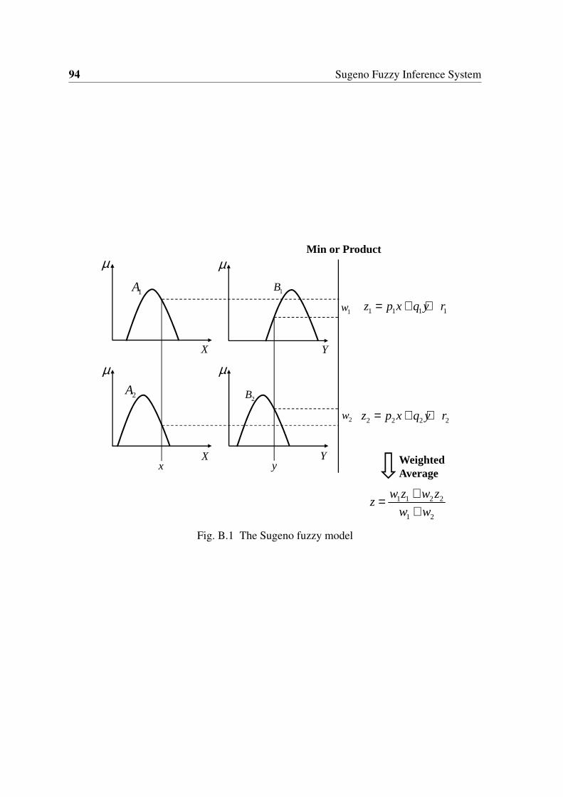
94 Sugeno Fuzzy Inference System
Min or Product
1 1 1 1z p x q y r= + +
2 2 2 2z p x q y r= + +
1w
2w
Y
Y
X
Xx y
µµ
µµ
1A 1B
2B2A
1 1 2 2
1 2
w z w zz
w w
+=+
Weighted Average
Fig. B.1 The Sugeno fuzzy model
Appendix C
Genetic Algorithms
A GA is a computational technique that simulates evolution in the search for solutions tocomplex problems. These are problems with large spaces of potential solutions, characterizedby nonlinearities. This means there is no linear relation between the performance of solutionsas classified along the dimensions used for characterizing them. If there were linear relations,the optimal solution could easily be found by a simple hill-climbing algorithm. A GAassesses the performance of different solutions in parallel and uses the information abouthow different solutions perform to direct the search towards promising areas of the searchspace. Adapting the search is done by simulating evolutionary processes.
Chromosome: A chromosome is the set of input variables for the GA. This can be consid-ered the genetic material constituting the solution you are solving for.
Population: The genetic population is a randomly generated group of chromosomes.
Fitness function: The fitness function is a performance index such that the fittest chromo-somes in the population will survive to the next generation. The fitter the parent, the greaterthe probability of selection for reproduction.
Fitness scaling: Fitness scaling converts the scores achieved from the fitness function to arange suitable for the function selected for reproduction.
Rank scaling: Rank scaling orders each individual according to their fitness, so that thestrongest comes first and the weakest last.
Fitness function tolerance: The fitness function tolerance defines the stopping conditionfor the genetic algorithm. When the change in the weighted fitness function value becomesless than the fitness function tolerance the genetic algorithm stops.
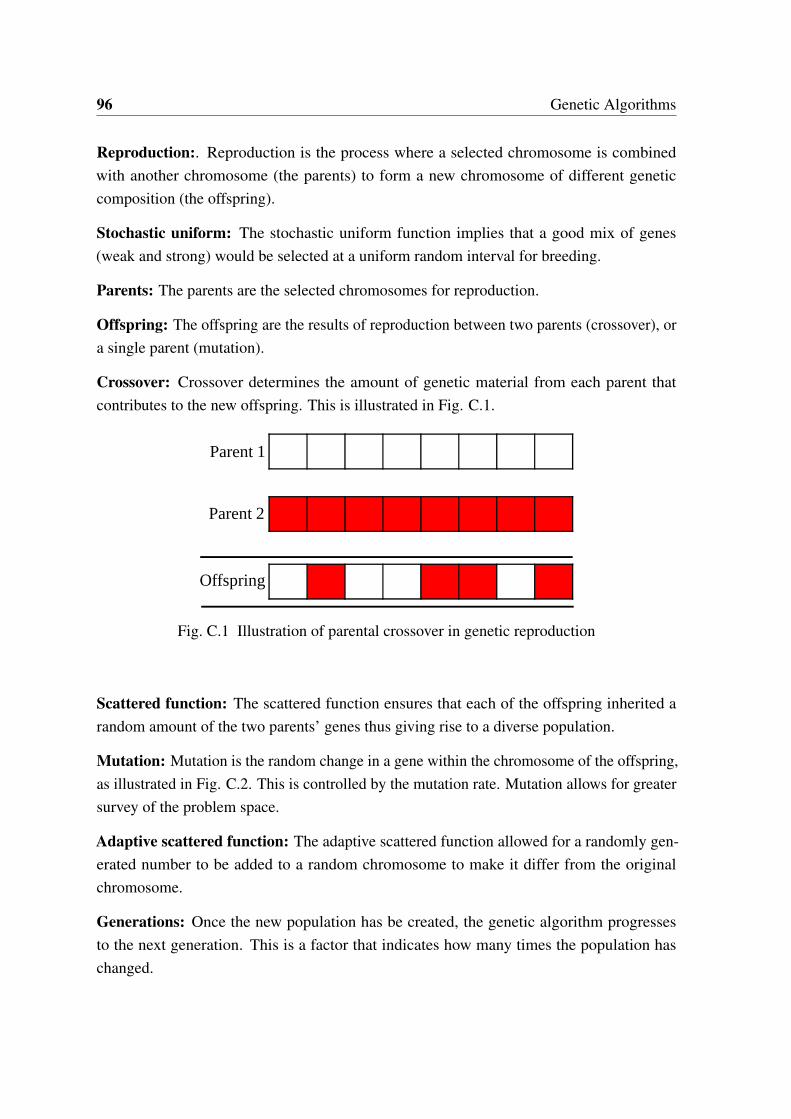
96 Genetic Algorithms
Reproduction:. Reproduction is the process where a selected chromosome is combinedwith another chromosome (the parents) to form a new chromosome of different geneticcomposition (the offspring).
Stochastic uniform: The stochastic uniform function implies that a good mix of genes(weak and strong) would be selected at a uniform random interval for breeding.
Parents: The parents are the selected chromosomes for reproduction.
Offspring: The offspring are the results of reproduction between two parents (crossover), ora single parent (mutation).
Crossover: Crossover determines the amount of genetic material from each parent thatcontributes to the new offspring. This is illustrated in Fig. C.1.
Parent 1
Parent 2
Offspring
Fig. C.1 Illustration of parental crossover in genetic reproduction
Scattered function: The scattered function ensures that each of the offspring inherited arandom amount of the two parents’ genes thus giving rise to a diverse population.
Mutation: Mutation is the random change in a gene within the chromosome of the offspring,as illustrated in Fig. C.2. This is controlled by the mutation rate. Mutation allows for greatersurvey of the problem space.
Adaptive scattered function: The adaptive scattered function allowed for a randomly gen-erated number to be added to a random chromosome to make it differ from the originalchromosome.
Generations: Once the new population has be created, the genetic algorithm progressesto the next generation. This is a factor that indicates how many times the population haschanged.
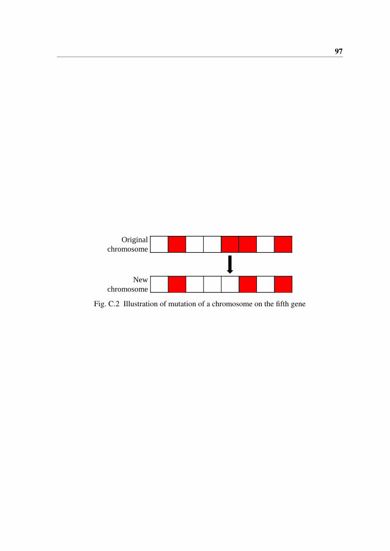
97
Original chromosome
New chromosome
Fig. C.2 Illustration of mutation of a chromosome on the fifth gene


![Learning a Fuzzy Controller by Genetic Algorithms · A fuzzy controller consists of a set of fuzzy control rules with appropriate inference mechanisms [1]. The fuzzy controller is](https://img.pdfslide.net/doc/110x75/5fdb09ef9cebd6099d5e2885/learning-a-fuzzy-controller-by-genetic-a-fuzzy-controller-consists-of-a-set-of-fuzzy.jpg)


![Medical Image Retrieval Using Fuzzy Connectedness Image ... · Medical Image Retrieval Using Fuzzy Connectedness Image Segmentation ... expectation maximization [4]-[6] algorithm](https://img.pdfslide.net/doc/110x75/5b7bb89f7f8b9a004b8d3109/medical-image-retrieval-using-fuzzy-connectedness-image-medical-image-retrieval.jpg)