Design of an Intelligent Manufacturing Scheduling and ... Yang Journal_Papers... · Design of an Intelligent Manufacturing Scheduling and Control System Using Fuzzy Logic: Sensitivity

M.A.S.Monfared/J.B.Yang

1

Design of an Intelligent Manufacturing Scheduling and Control System Using Fuzzy Logic: Sensitivity

Analysis and Parameter Optimization

M.A.S. Monfared Department of Industrial Engineering

The University of Alzahra, Tehran, Iran. [email protected]

J. B. Yang∗ Manchester School of Management, UMIST, Manchester M60 1QD, UK.

[email protected]

Abstract

In this paper techniques and concepts from fuzzy logic theory, control theory, and optimisation theory are integrated together, to provide a novel intelligent manufacturing control system that operates in real-time, and is capable of responding to both structural and order related disturbances in a fully automated manner. In this paper we further developed our previous research on a second order intelligent scheduling and control system by performing an extensive sensitivity analysis and parameter optimization in order to achieve a good and reliable control system.

Keywords

Intelligent Manufacturing, Fuzzy Predictive, Scheduling, Control System

∗

Corresponding author


2

1 Introduction

The complexity of a scheduling and control problem is to a great extent case specific

that is, it depends upon the given manufacturing system and also upon the level of detail

which is considered appropriate. Development of scheduling and control algorithms using

intelligent systems has recently attracted attentions from researchers in different disciplines

including operations researchers, control theorists and computer scientists.

Artiba and Aghezzaf [3] developed architecture of a multi-model based system for

production planning and scheduling. It integrates expert systems, discrete event simulation,

optimization algorithms and heuristics to support decision making for complex production

planning and scheduling problems. A chemical plant which produces herbicides from process

industry has been presented to illustrate the method. Once the aggregate plan is produced, the

scheduling level is then tackled. Here again some of the multi-model functionalities are

employed using different models (MILP, heuristics, rules, . . ). This loop is repeated until the

final result is satisfying or a fixed number of iterations is reached. The tools used to solve this

case are C+ + , SLAM II and Microsoft Excell. It takes about 5 minutes to get a solution on a

PC 486/66. The object- oriented approach is used for data modelling. The multi-model

approach is very promising for the solution of complex manufacturing problems.

Hong and Chuang [9] developed a new scheduling algorithm for a two-machine flow

shop manufacturing system where job processing time may vary dynamically. In the past, the

processing time for each job was usually assigned or estimated as a fixed value. In many real-

world applications, however, this is not practical. Fuzzy concepts were applied to Johnson

algorithm for managing uncertain process time scheduling. Given a set of jobs, each having

two tasks that must be executed on two machines, and their processing time membership

functions, the fuzzy Johnson algorithm can yield a scheduling result with a membership

function for the final completion time. The fuzzy Johnson algorithm can produce feasible

solutions for both deterministic and uncertain situations.


3

Devedzic and Radovic[7] developed a framework for building Intelligent

Manufacturing Systems (IMS). IMS contain software components using such techniques as

expert systems, fuzzy logic, neural networks, and machine learning. The number, the kind,

and the complexity of intelligent components of an IMS can vary a lot from one system to

another, and the components themselves can be combined in many ways, depending on the

application. Here again the emphasis is on software development similar to other cases

reviewed above.

Another important development is the emergence of Manufacturing Execution

System (MES). In the paradigm of a manufacturing automation hierarchy, MES is located in

the middle where Enterprise Resources Planning (ERP) system is located above and

Supervisory Control And Data Acquisition (SCADA) system is located below. SCADA

provides decision makings and control throughout the factory and controls Distributed

Control Systems (DCS) and Programmable Logic Controllers (PLC). See [5],[14],[22].

Shaout and McAuliffe [19] presented a batch job scheduler for a distributed system

which utilizes a fuzzy logic algorithm to balance the load on individual processors

maximizing throughput of the overall system. The fuzzy load balancing algorithm was

implemented in a real production setting showing improved performance and reliability

characteristics.

Hambaba [8] argued that the design and implementation of effective control of

manufacturing processes depends on the successful monitoring and recognition of process

signals and machine sensors. A hybrid architecture was developed to predict plasma etcher

outcome, etcher rate, selectivity, and uniformity. The architecture includes a robust model and

recurrent neural network with real-time recurrent learning. The residual errors were used to

tune the weights of the recurrent neural network.

Sapena and Onaindía [18] developed an integrated tool called SimPlanner for

planning and execution-monitoring in dynamic environment which allows to interleave


4

planning and execution. The on-line planner incorporated in SimPlanner is domain-

independent.

Researchers tend to agree that new tools, methods, and technologies must be

developed to address the specific situations and needs. Attempts to build general tools such as

MRP, ERP, MES (see [11], [14], [22]) and general methods (e.g., dispatching rules which

minimise multiple objectives) have essentially failed (see e.g., [1], [2], [4], [12], [13], [15],

[20], [23], [24]).

From the intensive research efforts that have been undertaken over the past 4 decades,

it is now evident that good tools, techniques and technologies need to be designed to fit the

specific system. However a methodology which is based on the integration of planning,

scheduling and control activities can be used to provide a platform for the design and

development of intelligent scheduling and control systems. An intelligent scheduling and

control system using queuing theory and fuzzy logic was developed in [16]. This paper

extends the results and develops the system further to include sensitivity analysis and

parameter optimization leading to new results.

The paper is organized as follows. In Section 2 an automated manufacturing system

configuration is described and a novel scheduling and control algorithm using fuzzy logic is

considered. The simulation results are also briefly reported to demonstrate the working

properties of the proposed algorithm. Section 3 provides sensitivity analysis and parameter

optimization for the proposed scheduling and control system. Performance analysis using

simulation experiments are reported in Section 4 and conclusions are drawn in Section 5.

2 Modelling an Automated Flow Shop System

A fully automated flow shop manufacturing system (or cell) is illustrated in Figure 1

which is considered for analysis and modelling purposes. This cell is formed by connecting

nine machines as follows: three robots for loading and unloading tasks, one conveyor belt for

handling incoming parts, three rotary spiral racks for storing parts, one heat treatment


5

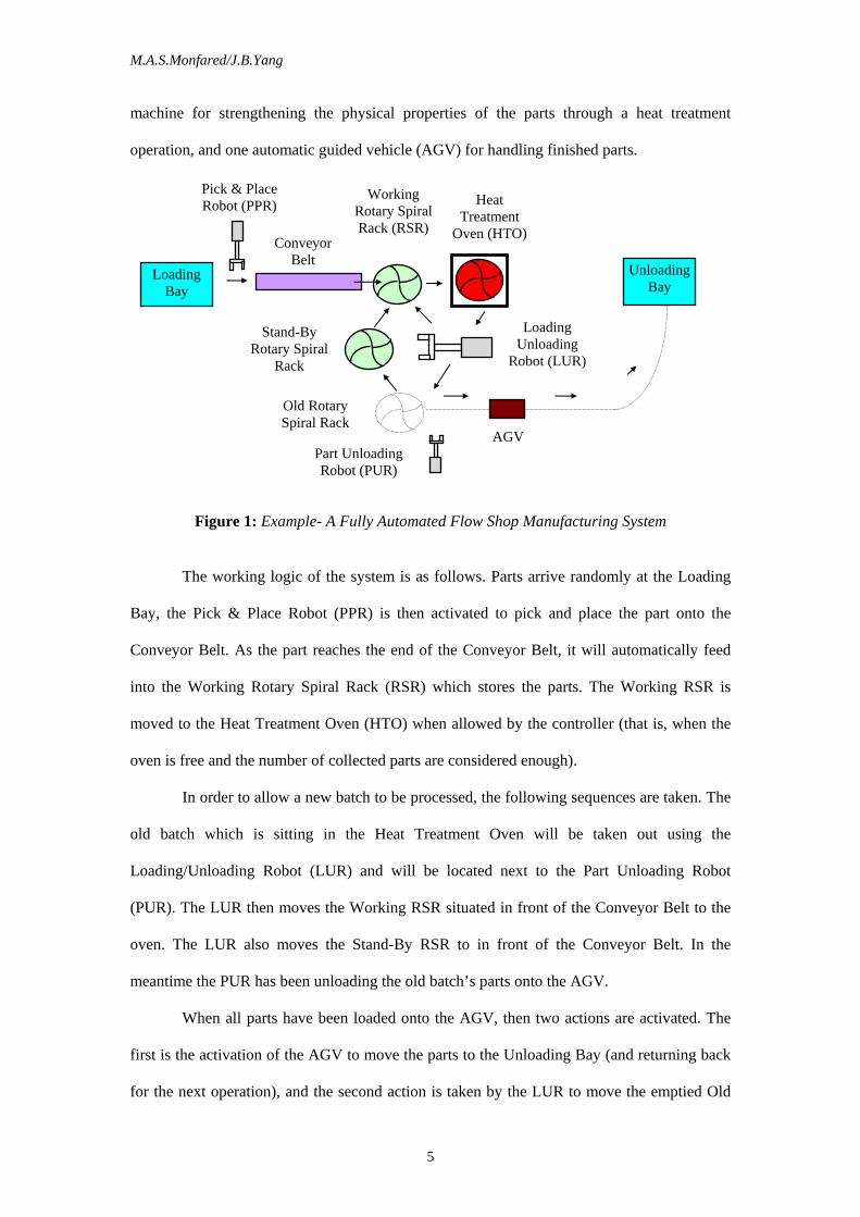
machine for strengthening the physical properties of the parts through a heat treatment

operation, and one automatic guided vehicle (AGV) for handling finished parts.

Figure 1: Example- A Fully Automated Flow Shop Manufacturing System

The working logic of the system is as follows. Parts arrive randomly at the Loading

Bay, the Pick & Place Robot (PPR) is then activated to pick and place the part onto the

Conveyor Belt. As the part reaches the end of the Conveyor Belt, it will automatically feed

into the Working Rotary Spiral Rack (RSR) which stores the parts. The Working RSR is

moved to the Heat Treatment Oven (HTO) when allowed by the controller (that is, when the

oven is free and the number of collected parts are considered enough).

In order to allow a new batch to be processed, the following sequences are taken. The

old batch which is sitting in the Heat Treatment Oven will be taken out using the

Loading/Unloading Robot (LUR) and will be located next to the Part Unloading Robot

(PUR). The LUR then moves the Working RSR situated in front of the Conveyor Belt to the

oven. The LUR also moves the Stand-By RSR to in front of the Conveyor Belt. In the

meantime the PUR has been unloading the old batch’s parts onto the AGV.

When all parts have been loaded onto the AGV, then two actions are activated. The

first is the activation of the AGV to move the parts to the Unloading Bay (and returning back

for the next operation), and the second action is taken by the LUR to move the emptied Old

Loading

Bay

Unloading Bay

Conveyor Belt

Pick & Place Robot (PPR)

Working Rotary Spiral Rack (RSR)

Heat Treatment

Oven (HTO)

Loading Unloading

Robot (LUR)

AGV Part Unloading Robot (PUR)

Stand-By Rotary Spiral

Rack

Old Rotary Spiral Rack


6

PSR to the stand-by position. All machines are of an on/off type except the Conveyor Belt,

which is permanently on. The times required for performing all operations are fixed except,

for the HTO processing time and the HTO part unloading time. These two operations are

variable because of the variations in the number of parts in a batch (that is a random variable).

It is this variability which makes the system different from so called conventional automated

systems. The system now is a stochastic dynamical system and is more sophisticated than a

conventional automated system due to the association of randomness.

2.1 A Stochastic Scheduling and Control System

The manufacturing system described in Figure 1 can be simplified as a queuing

system, where parts arrive randomly, accumulate in a queue and then receive service by a

single server. Since the parts are served in a batch wise fashion, this queuing system is

classified as a batch service queuing process (or single batch production system). The beauty

of the single batch processing system is that it provides a simple and straightforward

production control system whose control logic is very simple, while at the same time it poses

many challenges, as will be discussed in the following.

In a single batch production system, such as a heat treatment oven, parts arrive

dynamically in accordance to a certain distribution (e.g., Poisson). These parts are “collected”

in a batch form, to reach a level that is equal to a certain number (e.g., Q). The processing

time is defined by a certain distribution (e.g., negative exponential). Such a single batch

processing system can also be found in a transportation system, in the form of a shuttle

service between an airport terminal and a remote parking lot (or a transit bus station). In either

case, if the parts (or passengers) arrive deterministically, a scheduled service might be the

optimal policy.

An important contribution of Deb & Serfozo [6] was that they have shown that a

threshold structure in which at any given point in time and where X parts (or passengers) are

waiting in the system, a control limit offers an optimal scheduling and control policy. This, to


7

put it in simple terms, is that a batch of size X parts is processed if and only if X exceeds a

threshold limit, Q.

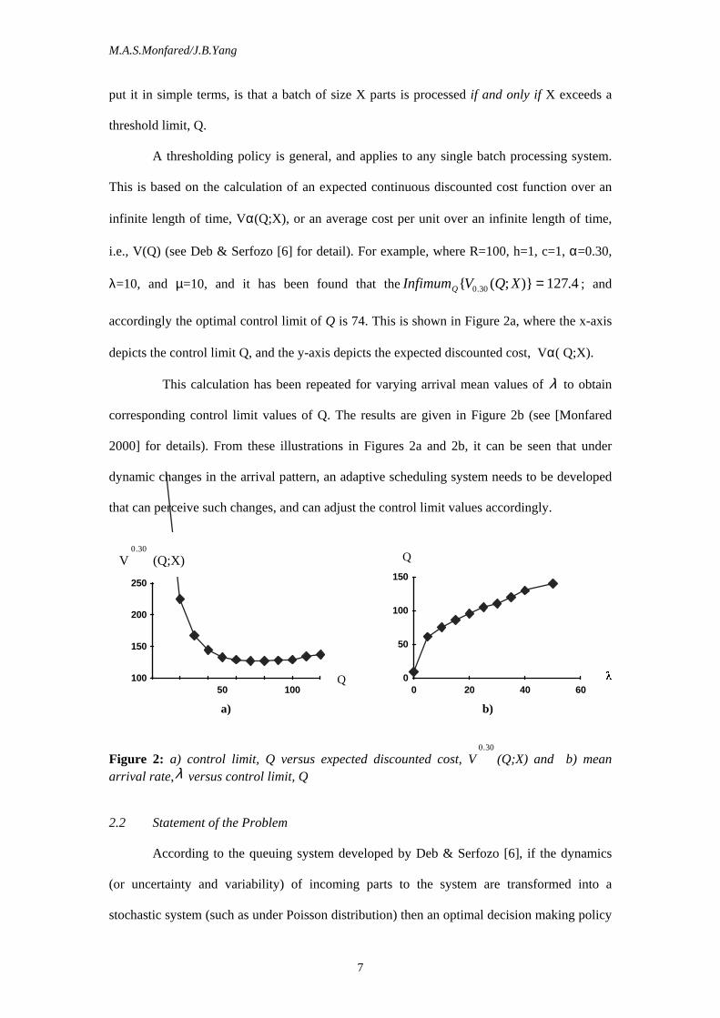
A thresholding policy is general, and applies to any single batch processing system.

This is based on the calculation of an expected continuous discounted cost function over an

infinite length of time, Vα(Q;X), or an average cost per unit over an infinite length of time,

i.e., V(Q) (see Deb & Serfozo [6] for detail). For example, where R=100, h=1, c=1, α=0.30,

λ=10, and µ=10, and it has been found that theInfimum V Q XQ ( ; ) .4.0 30 127= ; and

accordingly the optimal control limit of Q is 74. This is shown in Figure 2a, where the x-axis

depicts the control limit Q, and the y-axis depicts the expected discounted cost, Vα( Q;X).

This calculation has been repeated for varying arrival mean values of λ to obtain

corresponding control limit values of Q. The results are given in Figure 2b (see [Monfared

2000] for details). From these illustrations in Figures 2a and 2b, it can be seen that under

dynamic changes in the arrival pattern, an adaptive scheduling system needs to be developed

that can perceive such changes, and can adjust the control limit values accordingly.

100

150

200

250

50 100

0

50

100

150

0 20 40 60

Figure 2: a) control limit, Q versus expected discounted cost, V0 30.

(Q;X) and b) mean arrival rate,λ versus control limit, Q

2.2 Statement of the Problem

According to the queuing system developed by Deb & Serfozo [6], if the dynamics

(or uncertainty and variability) of incoming parts to the system are transformed into a

stochastic system (such as under Poisson distribution) then an optimal decision making policy

Q

Q

V0 30.

(Q;X)

a) b)


8

can be formulated. The question is, however, what if the dynamics available in this system

cannot be simplified to such a stochastic pattern.

It is clear that the validity of the optimal policy is conditioned by a number of

assumptions, one of which is that the population is stationary (i.e., the first and the second

moment are fixed in value). If stationary conditions are not met, then the optimality of the

policy will be lost. In the following, a non-stationary stochastic system is considered under

the following conditions:

1) the nature of the uncertainty in the incoming orders is random, i.e., no before-hand

information exists and an uncertainty structure, if there is any, must be only perceived

through the stream of data,

2) the frequency of non-stationary variability is considered low, so that for a certain

length of time the system under consideration is considered stationary (i.e., the system is

piece-wise stationary- in an analogy with piece-wise linear systems),

3) when the system is in its stationary mode, the incoming orders follow a Poisson

probability distribution.

Under these conditions, it is desired to develop an intelligent (i.e., adaptive) system,

where the control limit is not considered to be fixed. Instead, the control limit is considered as

a variable, to reflect the uncertainty in the pattern of part arrivals. The proposed intelligent

control system is presented next.

2.3 A New Scheduling and Control Algorithm

There are basically three forms of structuring planning, scheduling and control

systems: centralized, hierarchical, and heterarchical (also called distributed or cooperative).

The centralized structure employs a centralized computer to manage and maintain the records

of all planning, scheduling and control functions. Machines execute the commands released

from the centralized computer and then feed back the execution results.


9

In a hierarchical structure which might be strict or loose, there is a master/slave

relationship between two adjacent levels of systems. In strict sense, peer communication

between controllers at the same levels is not allowed. Within the hierarchy of systems, a

superior sees only its immediate subordinates and not the subordinates of its subordinates.

This concept gives each system a certain control authority within its realm.

Basically, loose hierarchical structure is similar to a strict hierarchical structure,

except that it allows peer communication. With this feature, the system structure has a loose

master/ slave relationship between system levels. A superior is responsible for initiating a

sequence of activities. The subordinates are able to cooperate to complete these activities in

sequence.

A heterarchical structure which is also called a distributed or cooperative structure

pursues the full local autonomy and a cooperative approach to global decision making. There

are no master/slave relationships between system components. Cooperation between

components is implemented via a negotiation and bidding procedure to accomplish tasks. The

heterarchical control architecture increases flexibility in operations at the price of higher

communication burden.

Meanwhile we consider that planning, scheduling and control functions can neither

be structured in centralized form nor in distributed form. This is due to inherent hierarchy

existed in such functions. It can therefore be considered as a collection of mechanisms for

treating system dynamics or disturbances is organized into a 3 level structure. At the lower

level the controller (i.e., C in Figure 3) is in direct contact with shop floor physical systems

such as machine centres, robots, and AGV’s, and controls these against disturbing events, Ω1.

At the middle layer, the scheduler (i.e., S in Figure 3) deals with order related events, Ω2.

Finally at the higher layer of the hierarchy, a planner (i.e., P in Figure 3) monitors long term

disturbing events, Ω3.

To treat a single disturbance, control theory has proposed a feedback control loop, as

illustrated in Figure 3, where the input to the controller is the desired schedule, and the


10

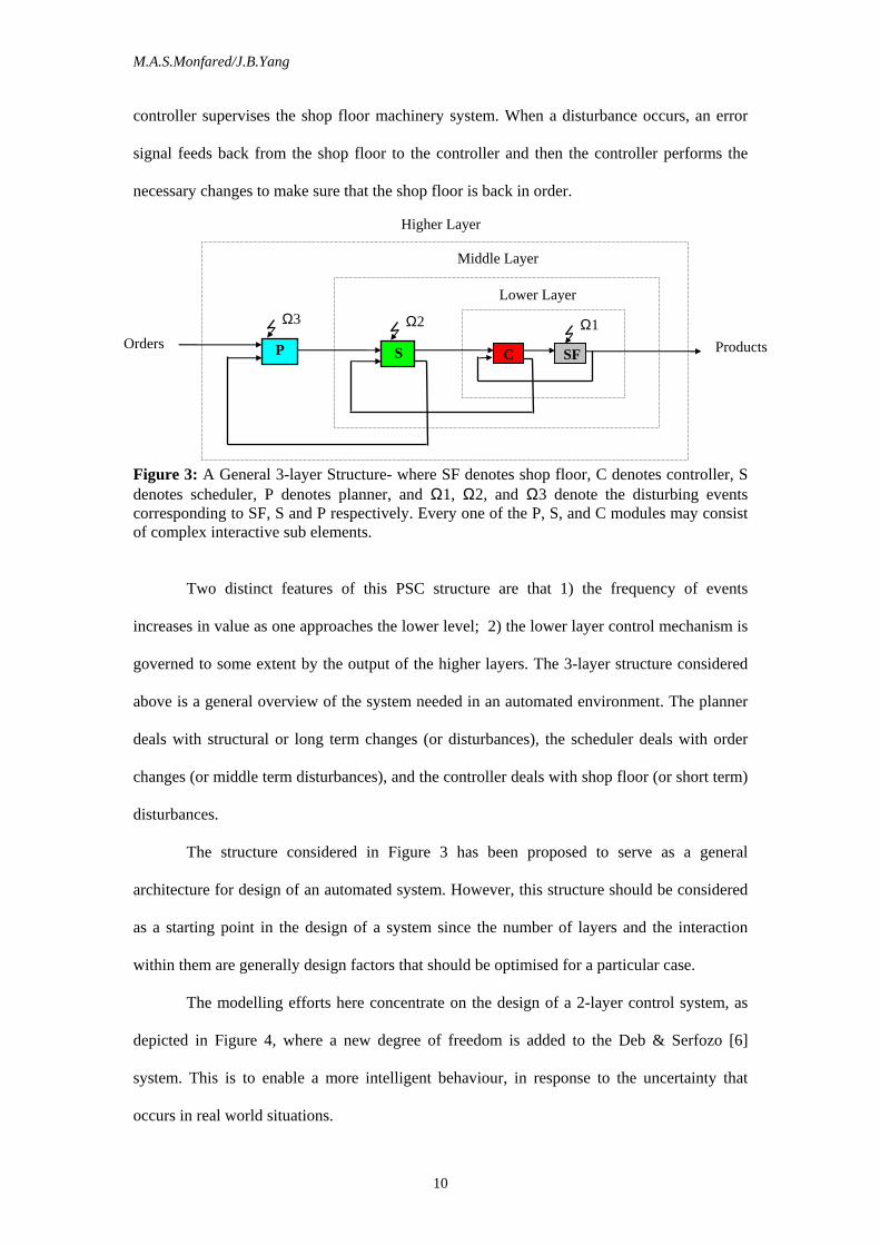
controller supervises the shop floor machinery system. When a disturbance occurs, an error

signal feeds back from the shop floor to the controller and then the controller performs the

necessary changes to make sure that the shop floor is back in order.

Figure 3: A General 3-layer Structure- where SF denotes shop floor, C denotes controller, S denotes scheduler, P denotes planner, and Ω1, Ω2, and Ω3 denote the disturbing events corresponding to SF, S and P respectively. Every one of the P, S, and C modules may consist of complex interactive sub elements.

Two distinct features of this PSC structure are that 1) the frequency of events

increases in value as one approaches the lower level; 2) the lower layer control mechanism is

governed to some extent by the output of the higher layers. The 3-layer structure considered

above is a general overview of the system needed in an automated environment. The planner

deals with structural or long term changes (or disturbances), the scheduler deals with order

changes (or middle term disturbances), and the controller deals with shop floor (or short term)

disturbances.

The structure considered in Figure 3 has been proposed to serve as a general

architecture for design of an automated system. However, this structure should be considered

as a starting point in the design of a system since the number of layers and the interaction

within them are generally design factors that should be optimised for a particular case.

The modelling efforts here concentrate on the design of a 2-layer control system, as

depicted in Figure 4, where a new degree of freedom is added to the Deb & Serfozo [6]

system. This is to enable a more intelligent behaviour, in response to the uncertainty that

occurs in real world situations.

C SF

Ω1

S

Ω2 Ω3

P

Lower Layer

Middle Layer

Higher Layer

Products Orders


11

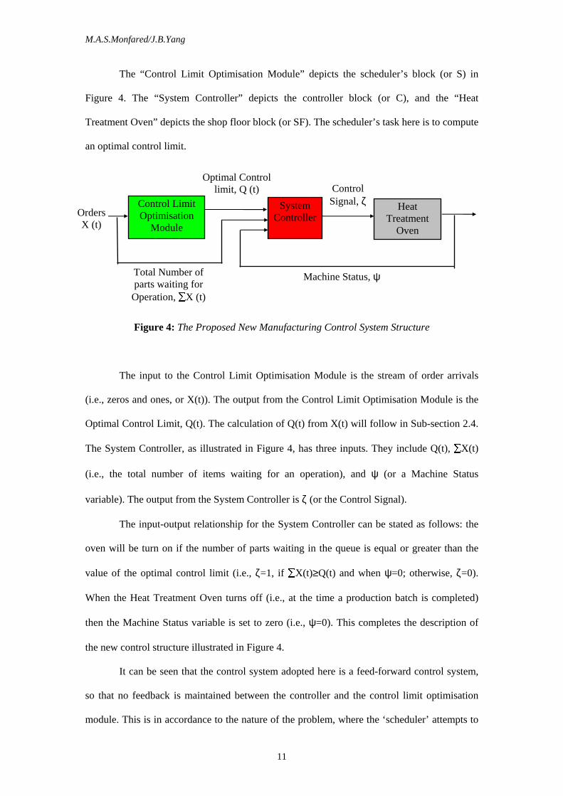
The “Control Limit Optimisation Module” depicts the scheduler’s block (or S) in

Figure 4. The “System Controller” depicts the controller block (or C), and the “Heat

Treatment Oven” depicts the shop floor block (or SF). The scheduler’s task here is to compute

an optimal control limit.

Figure 4: The Proposed New Manufacturing Control System Structure

The input to the Control Limit Optimisation Module is the stream of order arrivals

(i.e., zeros and ones, or X(t)). The output from the Control Limit Optimisation Module is the

Optimal Control Limit, Q(t). The calculation of Q(t) from X(t) will follow in Sub-section 2.4.

The System Controller, as illustrated in Figure 4, has three inputs. They include Q(t),

X(t)

(i.e., the total number of items waiting for an operation), and ψ (or a Machine Status

variable). The output from the System Controller is ζ (or the Control Signal).

The input-output relationship for the System Controller can be stated as follows: the

oven will be turn on if the number of parts waiting in the queue is equal or greater than the

value of the optimal control limit (i.e., ζ=1, if

X(t)≥Q(t) and when ψ=0; otherwise, ζ=0).

When the Heat Treatment Oven turns off (i.e., at the time a production batch is completed)

then the Machine Status variable is set to zero (i.e., ψ=0). This completes the description of

the new control structure illustrated in Figure 4.

It can be seen that the control system adopted here is a feed-forward control system,

so that no feedback is maintained between the controller and the control limit optimisation

module. This is in accordance to the nature of the problem, where the ‘scheduler’ attempts to

Control Signal, ζ

Optimal Control limit, Q (t)

Control Limit Optimisation

Module

System Controller

Heat Treatment

Oven

Orders X (t)

Total Number of parts waiting for Operation,

X (t)

Machine Status, ψ


12

find the optimal control limit policy based on the information acquired from the order

arrivals. The design of the Control Limit Optimisation Module, within the structure depicted

in Figure 4, improves the intelligence of the system. In fact, by deleting this module, the

system becomes the traditional control limit system of Deb & Serfozo [6].

2.4 Mathematical Structure of the Proposed System

The proposed adaptive system developed by the author can be considered as an

autonomous input-output function, whose input is the stream of parts (i.e., X(t)), and whose

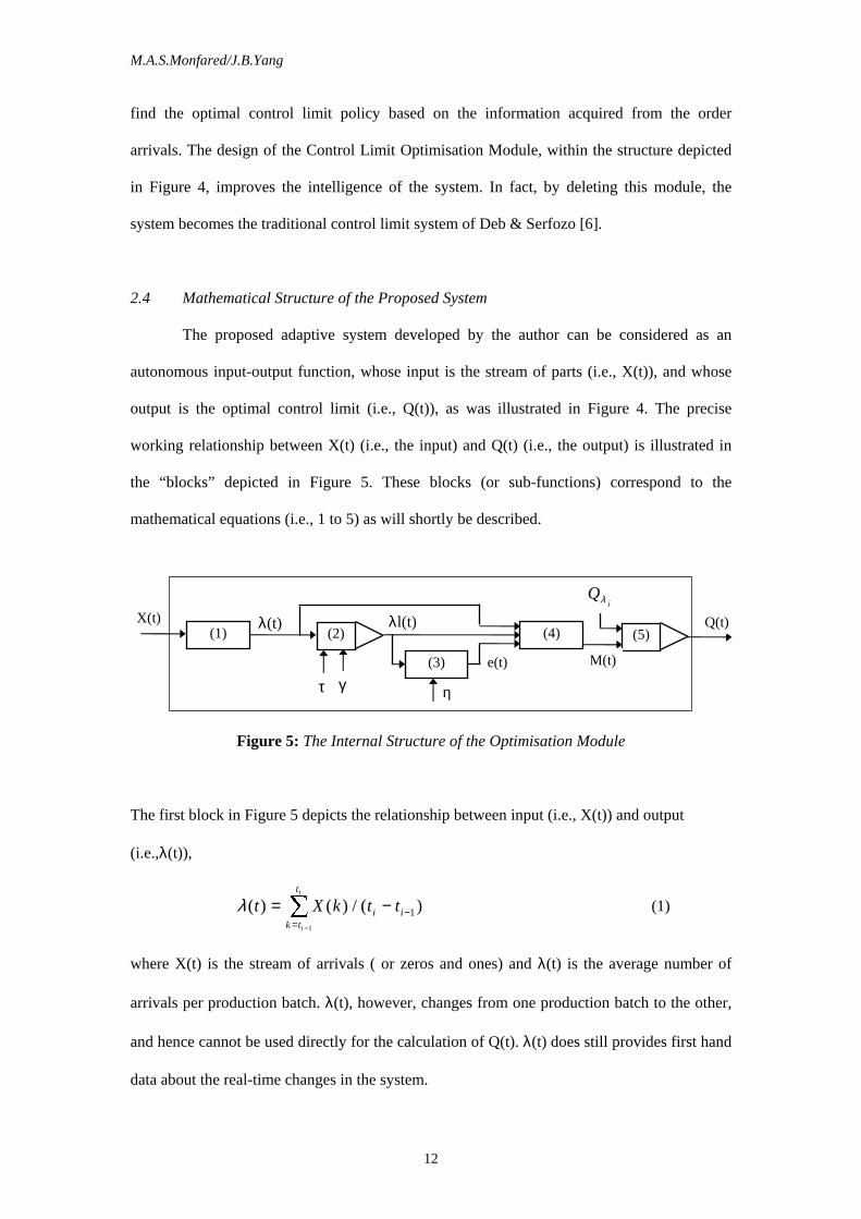
output is the optimal control limit (i.e., Q(t)), as was illustrated in Figure 4. The precise

working relationship between X(t) (i.e., the input) and Q(t) (i.e., the output) is illustrated in

the “blocks” depicted in Figure 5. These blocks (or sub-functions) correspond to the

mathematical equations (i.e., 1 to 5) as will shortly be described.

Figure 5: The Internal Structure of the Optimisation Module

The first block in Figure 5 depicts the relationship between input (i.e., X(t)) and output

(i.e.,λ(t)),

λ( ) ( ) / ( )t X k t tik t

t

i

i

i

= −=

−−

1

1 (1)

where X(t) is the stream of arrivals ( or zeros and ones) and λ(t) is the average number of

arrivals per production batch. λ(t), however, changes from one production batch to the other,

and hence cannot be used directly for the calculation of Q(t). λ(t) does still provides first hand

data about the real-time changes in the system.

(1) X(t) λ(t)

(2) λl(t)

(3)

(4) (5)

M(t)

Qjλ

e(t)

Q(t)

τ γ η


13

In order to estimate the actual λ, it is required to observe λ(t) for long enough a length

of time. This is the function of the second block in Figure 5, as defined in the following

equation;

λ λγ

γ

τ

τ

l t

e

e t nn

n t

tn

n t

t

i

i

i

i

( ) ( )= −−

=

−

=

−

−

1 (2)

If λ(t) is a simple moving average of the part arrivals within the batches i-1 and i,

then nλl(t), as in Equation (2), would represent an weighted moving average of the part

arrivals, X(t) as calculated over a longer period (τ periods or production batches), and when

the learning rate is γ. This weighted moving average has been derived by the author, and is re

termed to as an Exponential Filtering (EF) technique.

The term exponential has been adopted to depict the fact that weightings are not

equal, because they change exponentially. This is in contrast to the simple moving average

approach, in which all weightings are identical. The term filtering has been adopted to depict

two factors. The first factor is that this moving average is a low pass filter which filters out

most of the high frequencies exist in the signal (see [21]).

The second factor in calling this function an exponential filtering, is to distinguish it

from the classical exponential moving average (EMA) technique. It should be noted that the

EF technique is a moving average technique with two parameters (i.e.,γ and τ ), in comparison

with the EMA technique which is with one parameter, and hence EF presents more flexibility.

The reason for adopting an exponential weighted average as in Equation (2) is that it

gives more weight to recent information (i.e., λ(t)), and hence it helps to establish the actual λ

faster. This is an advantage when the underlying system is non-stationary.

The calculated value of λl(t) (as in Equation (2)) can be used now to estimate the

corresponding value for Q(t). This enables the control system to work adaptively with

changing λ. In order to increase the intelligence of the system and improve its adaptivity,

fuzzy theory is used, as illustrated in Equations (3) to (5) of Figure 5.


14

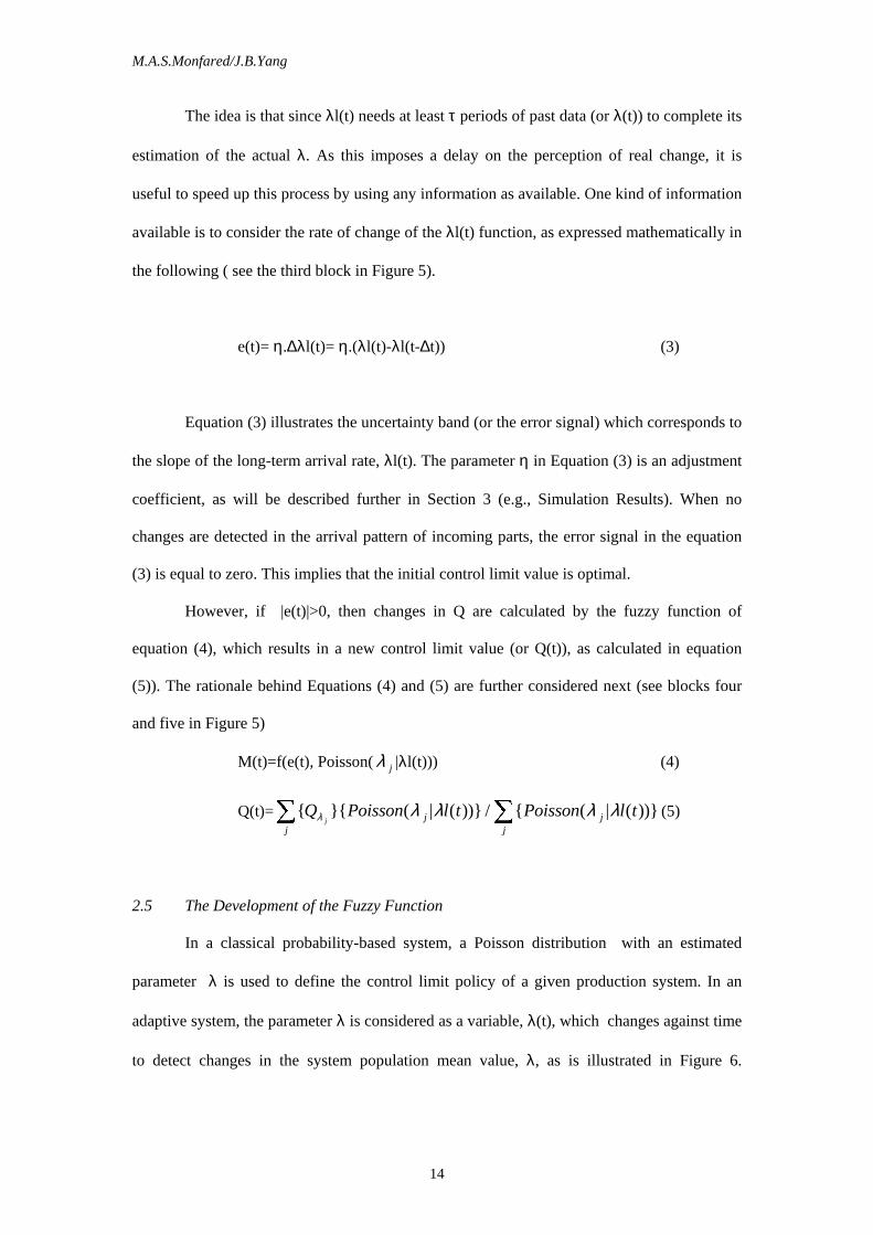
The idea is that since λl(t) needs at least τ periods of past data (or λ(t)) to complete its

estimation of the actual λ. As this imposes a delay on the perception of real change, it is

useful to speed up this process by using any information as available. One kind of information

available is to consider the rate of change of the λl(t) function, as expressed mathematically in

the following ( see the third block in Figure 5).

e(t)= η.∆λl(t)= η.(λl(t)-λl(t-∆t)) (3)

Equation (3) illustrates the uncertainty band (or the error signal) which corresponds to

the slope of the long-term arrival rate, λl(t). The parameter η in Equation (3) is an adjustment

coefficient, as will be described further in Section 3 (e.g., Simulation Results). When no

changes are detected in the arrival pattern of incoming parts, the error signal in the equation

(3) is equal to zero. This implies that the initial control limit value is optimal.

However, if |e(t)|>0, then changes in Q are calculated by the fuzzy function of

equation (4), which results in a new control limit value (or Q(t)), as calculated in equation

(5)). The rationale behind Equations (4) and (5) are further considered next (see blocks four

and five in Figure 5)

M(t)=f(e(t), Poisson( λ j |λl(t))) (4)

Q(t)= ( | ( )) / ( | ( ))Q Poisson l t Poisson l tj j j

jjλ λ λ λ λ

(5)

2.5 The Development of the Fuzzy Function

In a classical probability-based system, a Poisson distribution with an estimated

parameter λ is used to define the control limit policy of a given production system. In an

adaptive system, the parameter λ is considered as a variable, λ(t), which changes against time

to detect changes in the system population mean value, λ, as is illustrated in Figure 6.


15

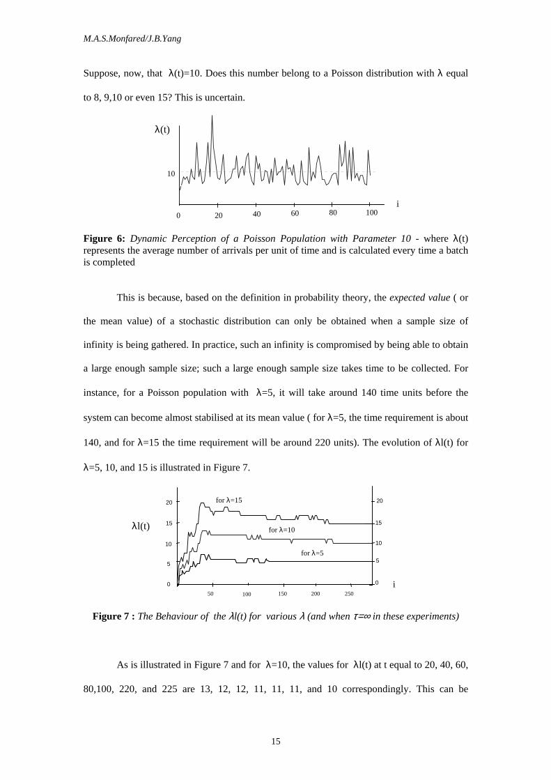
Suppose, now, that λ(t)=10. Does this number belong to a Poisson distribution with λ equal

to 8, 9,10 or even 15? This is uncertain.

0 20 40 60 80 100

10

Figure 6: Dynamic Perception of a Poisson Population with Parameter 10 - where λ(t) represents the average number of arrivals per unit of time and is calculated every time a batch is completed

This is because, based on the definition in probability theory, the expected value ( or

the mean value) of a stochastic distribution can only be obtained when a sample size of

infinity is being gathered. In practice, such an infinity is compromised by being able to obtain

a large enough sample size; such a large enough sample size takes time to be collected. For

instance, for a Poisson population with λ=5, it will take around 140 time units before the

system can become almost stabilised at its mean value ( for λ=5, the time requirement is about

140, and for λ=15 the time requirement will be around 220 units). The evolution of λl(t) for

λ=5, 10, and 15 is illustrated in Figure 7.

0

5

15

20

0

5

10

15

20

10

50 100 150 200 250

Figure 7 : The Behaviour of the λl(t) for various λ (and when τ=∞ in these experiments)

As is illustrated in Figure 7 and for λ=10, the values for λl(t) at t equal to 20, 40, 60,

80,100, 220, and 225 are 13, 12, 12, 11, 11, 11, and 10 correspondingly. This can be

λ(t)

λl(t)

i

for λ=15

for λ=10

for λ=5

i


16

considered as the first type of uncertainty that is available in this system. To obtain a stable

λl(t), enough time has to be spent in collecting data to be able to perceive the real mean value

of the given system. The validity of such a perception is, however, subject to the fact that the

system must not be exposed to any changes in its own mean value (i.e., it must be a stationary

system).

If the system is (in general) non-stationary, meaning that the population mean value is

changing from time to time, then it is almost impossible to collect data for a enough time, and

hence to perceive the mean value afterward. This uncertainty that originates from the

evolutionary nature of the situation can hardly be represented in the frame work of stochastic

theory.

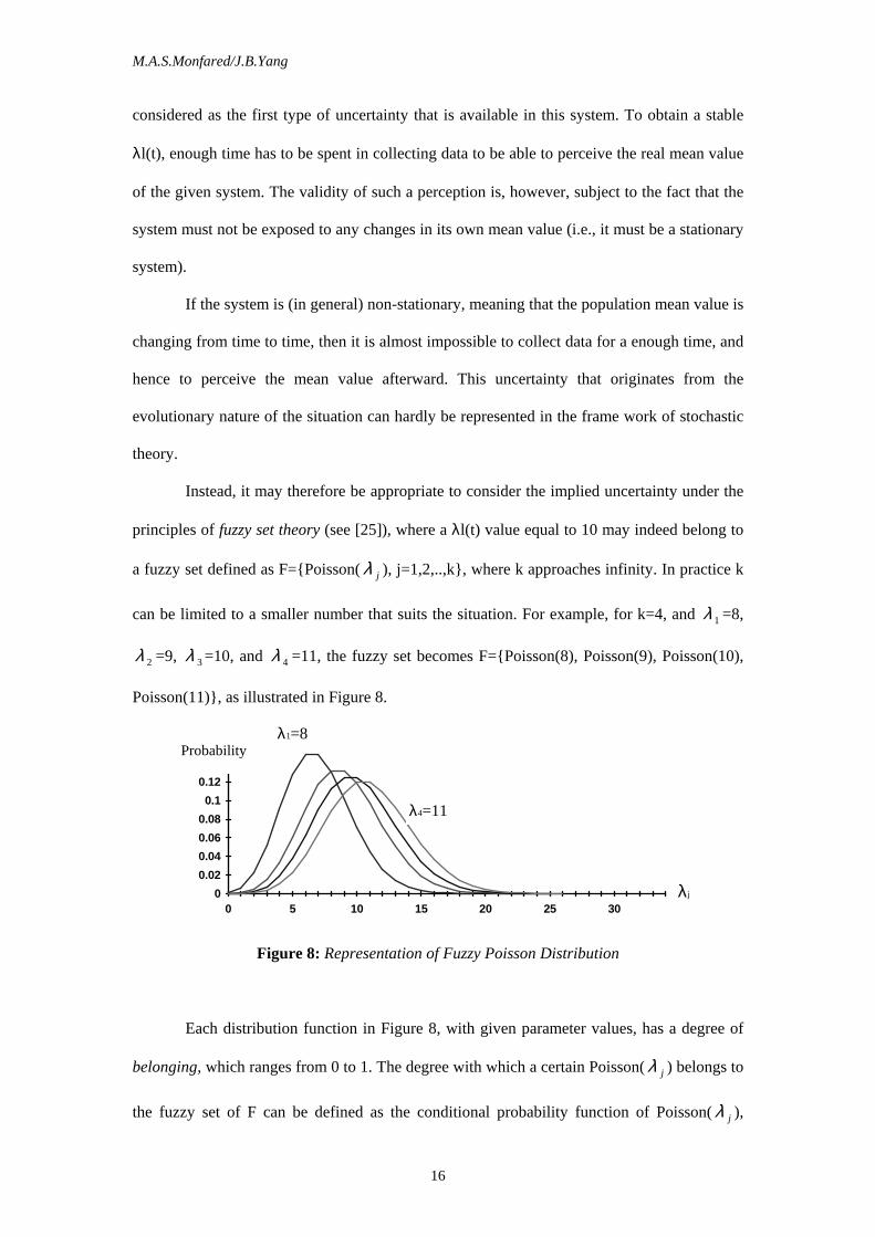
Instead, it may therefore be appropriate to consider the implied uncertainty under the

principles of fuzzy set theory (see [25]), where a λl(t) value equal to 10 may indeed belong to

a fuzzy set defined as F= Poisson( λ j ), j=1,2,..,k , where k approaches infinity. In practice k

can be limited to a smaller number that suits the situation. For example, for k=4, and λ 1 =8,

λ 2 =9, λ 3=10, and λ 4 =11, the fuzzy set becomes F= Poisson(8), Poisson(9), Poisson(10),

Poisson(11) , as illustrated in Figure 8.

0

0.02

0.04

0.06

0.08

0.1

0.12

0.14

0.16

0 5 10 15 20 25 30

Figure 8: Representation of Fuzzy Poisson Distribution

Each distribution function in Figure 8, with given parameter values, has a degree of

belonging, which ranges from 0 to 1. The degree with which a certain Poisson( λ j ) belongs to

the fuzzy set of F can be defined as the conditional probability function of Poisson( λ j ),

λj

Probability λ1=8

λ4=11


17

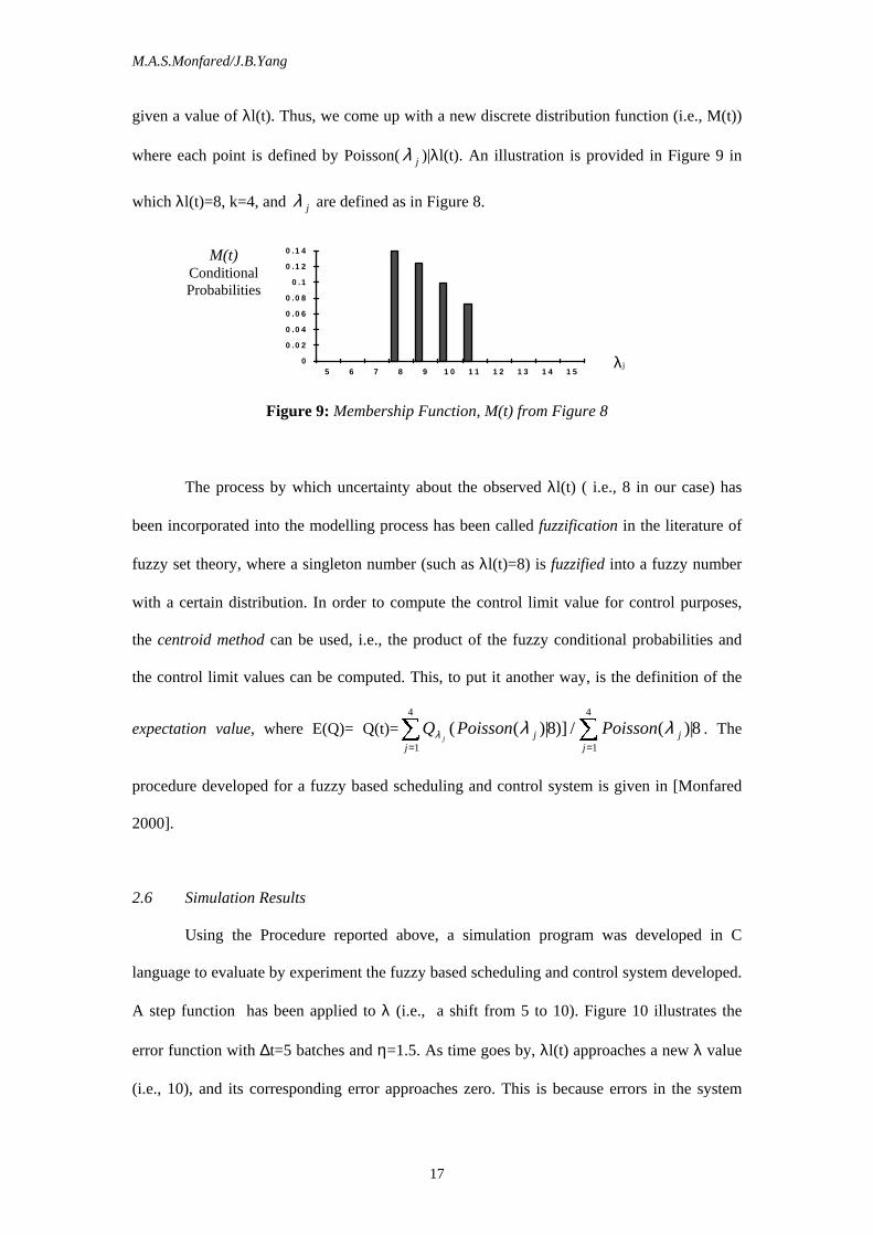
given a value of λl(t). Thus, we come up with a new discrete distribution function (i.e., M(t))

where each point is defined by Poisson( λ j )|λl(t). An illustration is provided in Figure 9 in

which λl(t)=8, k=4, and λ j are defined as in Figure 8.

0

0 .0 2

0 .0 4

0 .0 6

0 .0 8

0 .1

0 .1 2

0 .1 4

5 6 7 8 9 1 0 1 1 1 2 1 3 1 4 1 5

Figure 9: Membership Function, M(t) from Figure 8

The process by which uncertainty about the observed λl(t) ( i.e., 8 in our case) has

been incorporated into the modelling process has been called fuzzification in the literature of

fuzzy set theory, where a singleton number (such as λl(t)=8) is fuzzified into a fuzzy number

with a certain distribution. In order to compute the control limit value for control purposes,

the centroid method can be used, i.e., the product of the fuzzy conditional probabilities and

the control limit values can be computed. This, to put it another way, is the definition of the

expectation value, where E(Q)= Q(t)= Q Poisson Poissonj j j

jjλ λ λ( ( )| )] / ( )|8 8

1

4

1

4

==

. The

procedure developed for a fuzzy based scheduling and control system is given in [Monfared

2000].

2.6 Simulation Results

Using the Procedure reported above, a simulation program was developed in C

language to evaluate by experiment the fuzzy based scheduling and control system developed.

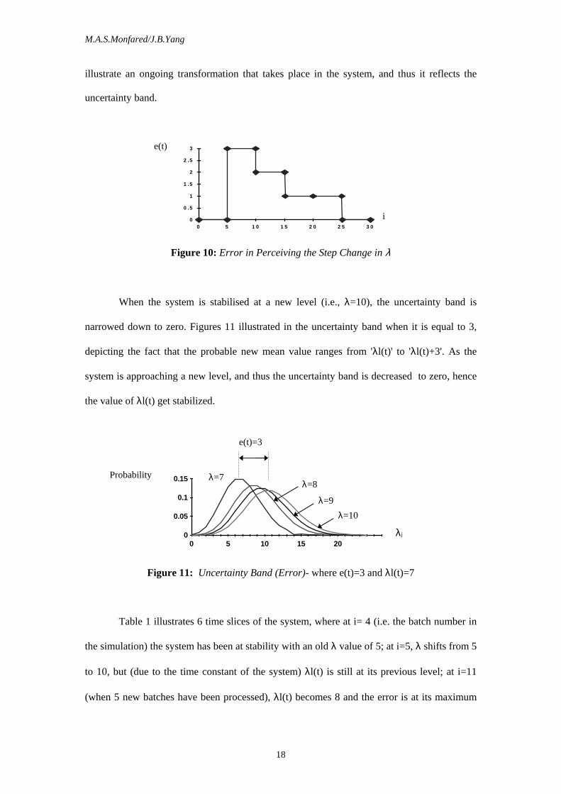
A step function has been applied to λ (i.e., a shift from 5 to 10). Figure 10 illustrates the

error function with ∆t=5 batches and η=1.5. As time goes by, λl(t) approaches a new λ value

(i.e., 10), and its corresponding error approaches zero. This is because errors in the system

M(t) Conditional Probabilities

λj


18

illustrate an ongoing transformation that takes place in the system, and thus it reflects the

uncertainty band.

0

0 .5

1

1 .5

2

2 .5

3

0 5 1 0 1 5 2 0 2 5 3 0

Figure 10: Error in Perceiving the Step Change in λ

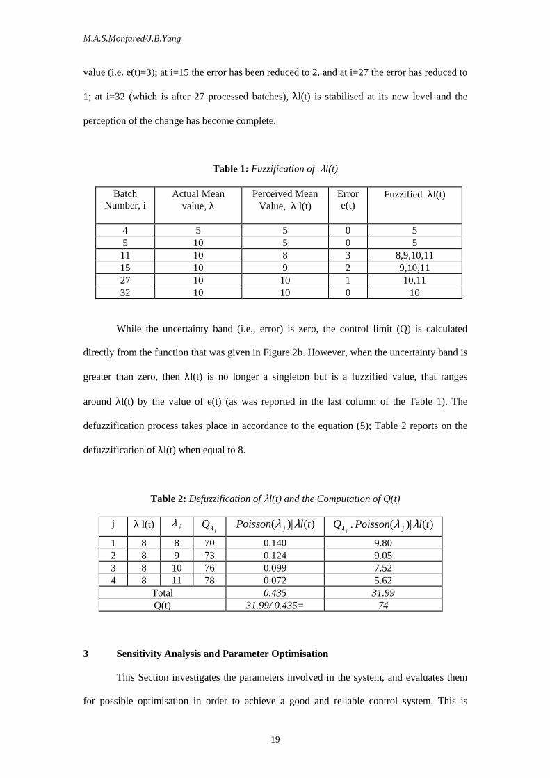
When the system is stabilised at a new level (i.e., λ=10), the uncertainty band is

narrowed down to zero. Figures 11 illustrated in the uncertainty band when it is equal to 3,

depicting the fact that the probable new mean value ranges from 'λl(t)' to 'λl(t)+3'. As the

system is approaching a new level, and thus the uncertainty band is decreased to zero, hence

the value of λl(t) get stabilized.

0

0.05

0.1

0.15

0 5 10 15 20

Figure 11: Uncertainty Band (Error)- where e(t)=3 and λl(t)=7

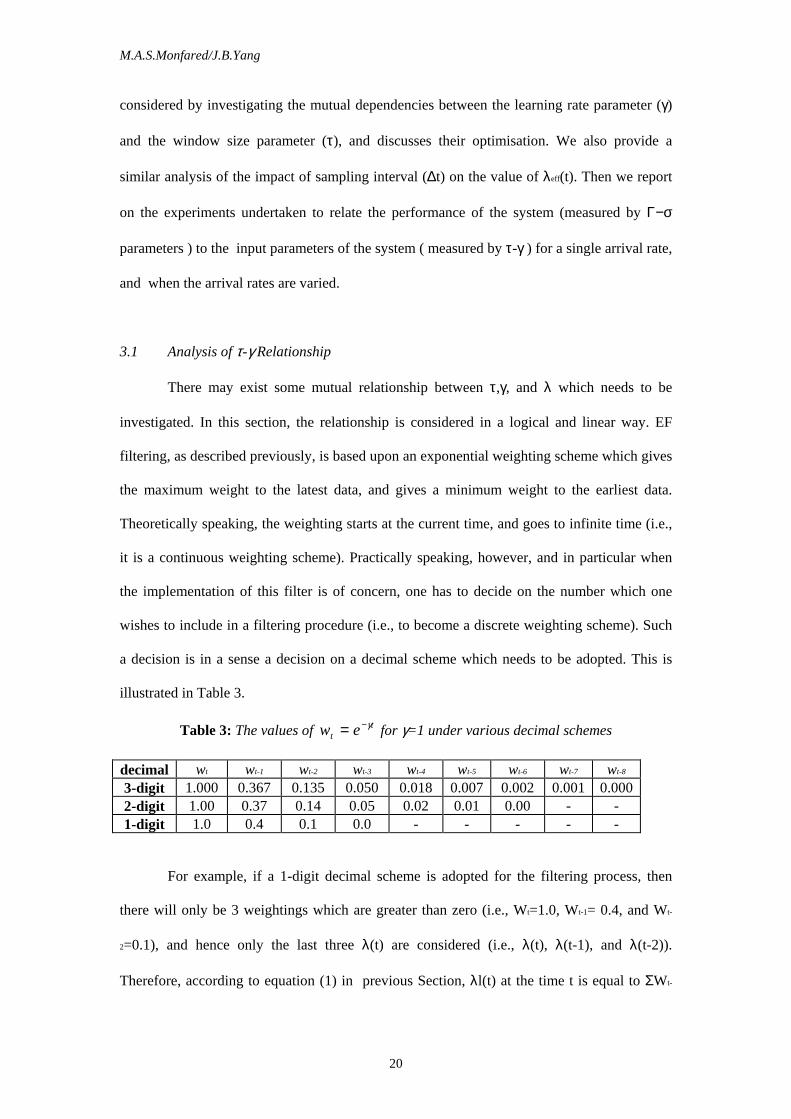
Table 1 illustrates 6 time slices of the system, where at i= 4 (i.e. the batch number in

the simulation) the system has been at stability with an old λ value of 5; at i=5, λ shifts from 5

to 10, but (due to the time constant of the system) λl(t) is still at its previous level; at i=11

(when 5 new batches have been processed), λl(t) becomes 8 and the error is at its maximum

λj

Probability

i

e(t)

λ=10

λ=9

λ=8 λ=7

e(t)=3


19

value (i.e. e(t)=3); at i=15 the error has been reduced to 2, and at i=27 the error has reduced to

1; at i=32 (which is after 27 processed batches), λl(t) is stabilised at its new level and the

perception of the change has become complete.

Table 1: Fuzzification of λl(t)

Batch Number, i

Actual Mean value, λ

Perceived Mean Value, λ l(t)

Error e(t)

Fuzzified λl(t)

4 5 5 0 5 5 10 5 0 5 11 10 8 3 8,9,10,11 15 10 9 2 9,10,11 27 10 10 1 10,11 32 10 10 0 10

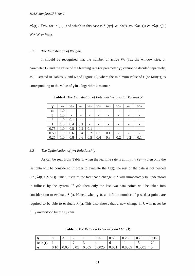
While the uncertainty band (i.e., error) is zero, the control limit (Q) is calculated

directly from the function that was given in Figure 2b. However, when the uncertainty band is

greater than zero, then λl(t) is no longer a singleton but is a fuzzified value, that ranges

around λl(t) by the value of e(t) (as was reported in the last column of the Table 1). The

defuzzification process takes place in accordance to the equation (5); Table 2 reports on the

defuzzification of λl(t) when equal to 8.

Table 2: Defuzzification of λl(t) and the Computation of Q(t)

j λ l(t) λ j Q

jλ Poisson l tj( )| ( )λ λ Qjλ . Poisson l tj( )| ( )λ λ

1 8 8 70 0.140 9.80 2 8 9 73 0.124 9.05 3 8 10 76 0.099 7.52 4 8 11 78 0.072 5.62

Total 0.435 31.99 Q(t) 31.99/ 0.435= 74

3 Sensitivity Analysis and Parameter Optimisation

This Section investigates the parameters involved in the system, and evaluates them

for possible optimisation in order to achieve a good and reliable control system. This is


20

considered by investigating the mutual dependencies between the learning rate parameter (γ)

and the window size parameter (τ), and discusses their optimisation. We also provide a

similar analysis of the impact of sampling interval (∆t) on the value of λeff(t). Then we report

on the experiments undertaken to relate the performance of the system (measured by Γ−σ

parameters ) to the input parameters of the system ( measured by τ-γ ) for a single arrival rate,

and when the arrival rates are varied.

3.1 Analysis of τ-γ Relationship

There may exist some mutual relationship between τ,γ, and λ which needs to be

investigated. In this section, the relationship is considered in a logical and linear way. EF

filtering, as described previously, is based upon an exponential weighting scheme which gives

the maximum weight to the latest data, and gives a minimum weight to the earliest data.

Theoretically speaking, the weighting starts at the current time, and goes to infinite time (i.e.,

it is a continuous weighting scheme). Practically speaking, however, and in particular when

the implementation of this filter is of concern, one has to decide on the number which one

wishes to include in a filtering procedure (i.e., to become a discrete weighting scheme). Such

a decision is in a sense a decision on a decimal scheme which needs to be adopted. This is

illustrated in Table 3.

Table 3: The values of w ett= −γ for γ=1 under various decimal schemes

decimal wt wt-1 wt-2 wt-3 wt-4 wt-5 wt-6 wt-7 wt-8 3-digit 1.000 0.367 0.135 0.050 0.018 0.007 0.002 0.001 0.000 2-digit 1.00 0.37 0.14 0.05 0.02 0.01 0.00 - - 1-digit 1.0 0.4 0.1 0.0 - - - - -

For example, if a 1-digit decimal scheme is adopted for the filtering process, then

there will only be 3 weightings which are greater than zero (i.e., Wt=1.0, Wt-1= 0.4, and Wt-

2=0.1), and hence only the last three λ(t) are considered (i.e., λ(t), λ(t-1), and λ(t-2)).

Therefore, according to equation (1) in previous Section, λl(t) at the time t is equal to ΣWt-


21

i*λ(t) / ΣWt-i for i=0,1,.. and which in this case is λl(t)=[ Wt *λ(t)+Wt-1*λ(t-1)+Wt-2*λ(t-2)]/(

Wt+ Wt-1+ Wt-2).

3.2 The Distribution of Weights

It should be recognised that the number of active Wt (i.e., the window size, or

parameter τ) and the value of the learning rate (or parameter γ ) cannot be decided separately,

as illustrated in Tables 5, and 6 and Figure 12, where the minimum value of τ (or Min(τ)) is

corresponding to the value of γ in a logarithmic manner.

Table 4: The Distribution of Potential Weights for Various γ

γγγγ wt wt-1 wt-2 wt-3 wt-4 wt-5 wt-6 wt-7 wt-8 ∞ 1.0 - - - - - - - - 3 1.0 - - - - - - - - 2 1.0 0.1 - - - - - - - 1 1.0 0.4 0.1 - - - - - -

0.75 1.0 0.5 0.2 0.1 - - - - - 0.50 1.0 0.6 0.4 0.2 0.1 0.1 - - - 0.25 1.0 0.8 0.6 0.5 0.4 0.3 0.2 0.2 0.1

3.3 The Optimisation of γ−τ Relationship

As can be seen from Table 5, when the learning rate is at infinity (γ=∞) then only the

last data will be considered in order to evaluate the λl(t); the rest of the data is not needed

(i.e., λl(t)= λ(t-1)). This illustrates the fact that a change in λ will immediately be understood

in fullness by the system. If γ=2, then only the last two data points will be taken into

consideration to evaluate λl(t). Hence, when γ=0, an infinite number of past data points are

required to be able to evaluate λl(t). This also shows that a new change in λ will never be

fully understood by the system.

Table 5: The Relation Between γ and Min(τ)

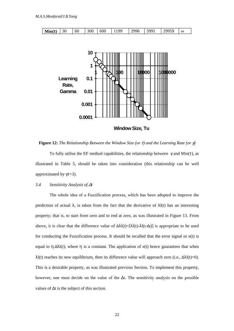
γγγγ ∞ 3 2 1 0.75 0.50 0.25 0.20 0.15 Min(ττττ) 1 1 2 3 4 6 11 15 20 γγγγ 0.10 0.05 0.01 0.005 0.0025 0.001 0.0005 0.0001 0


22

Min(ττττ) 30 60 300 600 1199 2996 5991 29959 ∞

Window Size, Tu

LearningRate,

Gamma

0.0001

0.001

0.01

0.1

1

10

1 100 10000 1000000

Figure 12: The Relationship Between the Window Size (or τ) and the Learning Rate (or γ)

To fully utilise the EF method capabilities, the relationship between γ and Min(τ), as

illustrated in Table 5, should be taken into consideration (this relationship can be well

approximated by γτ=3).

3.4 Sensitivity Analysis of ∆t

The whole idea of a Fuzzification process, which has been adopted to improve the

prediction of actual λ, is taken from the fact that the derivative of λl(t) has an interesting

property; that is, to start from zero and to end at zero, as was illustrated in Figure 13. From

above, it is clear that the difference value of ∆λl(t)=[λl(t)-λl(t-∆t)] is appropriate to be used

for conducting the Fuzzification process. It should be recalled that the error signal or e(t) is

equal to η.∆λl(t), where η is a constant. The application of e(t) hence guarantees that when

λl(t) reaches its new equilibrium, then its difference value will approach zero (i.e., ∆λl(t)=0).

This is a desirable property, as was illustrated previous Section. To implement this property,

however, one must decide on the value of the ∆t. The sensitivity analysis on the possible

values of ∆t is the subject of this section.


23

3.4 The Optimum ∆t

The purpose here is to examine whether a change in ∆t would have any impact on the

quality of the Fuzzification procedure. It is ideal to reproduce a derivative curve as smooth as

possible. This is practically impossible because of the nature of the dynamic system which is

random, and hence causes λl(t) to fluctuate. Although a proper selection of γ−τ will reduce

the fluctuation, it never cause the λl(t) to be a fully smooth curve.

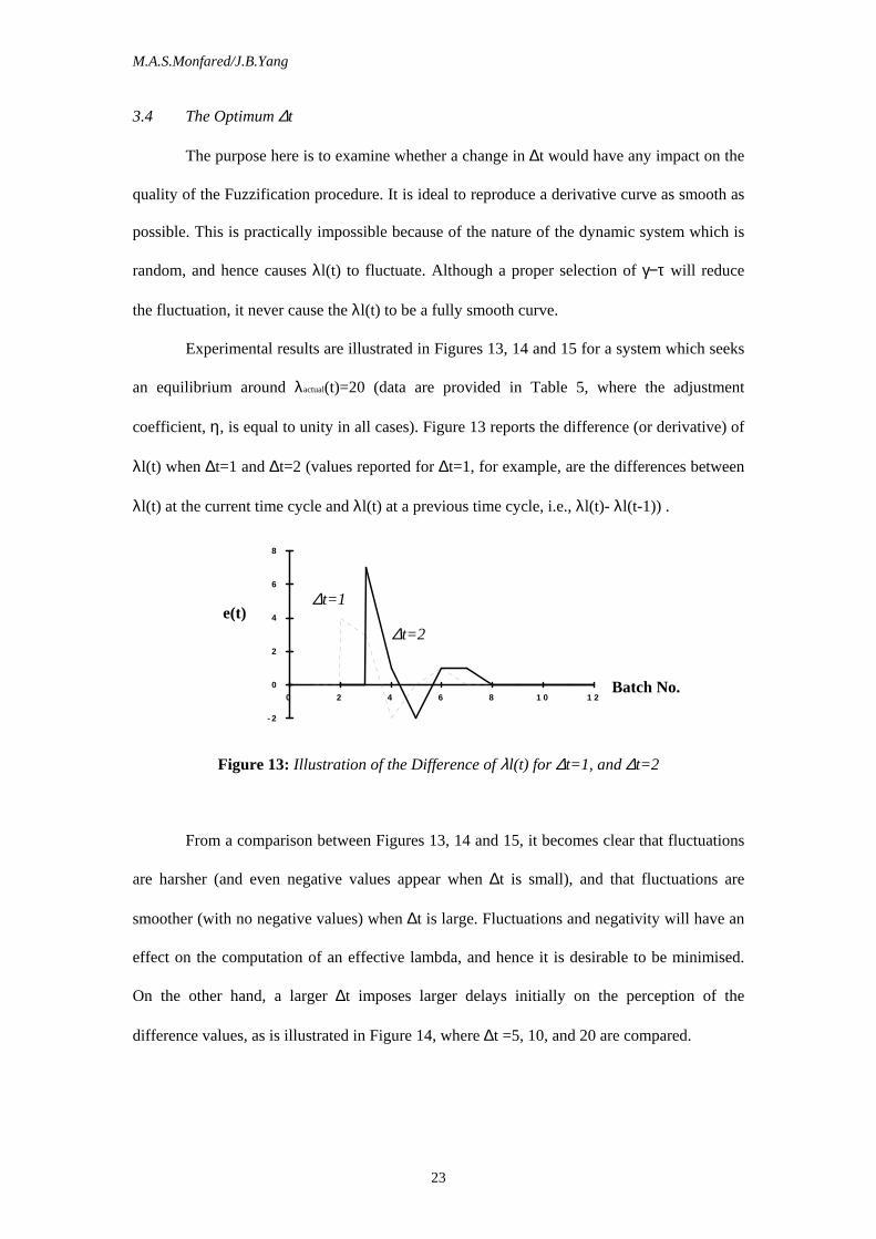
Experimental results are illustrated in Figures 13, 14 and 15 for a system which seeks

an equilibrium around λactual(t)=20 (data are provided in Table 5, where the adjustment

coefficient, η, is equal to unity in all cases). Figure 13 reports the difference (or derivative) of

λl(t) when ∆t=1 and ∆t=2 (values reported for ∆t=1, for example, are the differences between

λl(t) at the current time cycle and λl(t) at a previous time cycle, i.e., λl(t)- λl(t-1)) .

- 2

0

2

4

6

8

0 2 4 6 8 1 0 1 2

Figure 13: Illustration of the Difference of λl(t) for ∆t=1, and ∆t=2

From a comparison between Figures 13, 14 and 15, it becomes clear that fluctuations

are harsher (and even negative values appear when ∆t is small), and that fluctuations are

smoother (with no negative values) when ∆t is large. Fluctuations and negativity will have an

effect on the computation of an effective lambda, and hence it is desirable to be minimised.

On the other hand, a larger ∆t imposes larger delays initially on the perception of the

difference values, as is illustrated in Figure 14, where ∆t =5, 10, and 20 are compared.

∆t=1 e(t)

Batch No.

∆t=2


24

-2

0

2

4

6

8

10

0 10 20 30 40

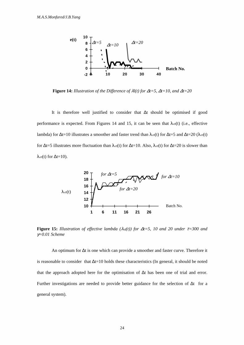
Figure 14: Illustration of the Difference of λl(t) for ∆t=5, ∆t=10, and ∆t=20

It is therefore well justified to consider that ∆t should be optimised if good

performance is expected. From Figures 14 and 15, it can be seen that λeff(t) (i.e., effective

lambda) for ∆t=10 illustrates a smoother and faster trend than λeff(t) for ∆t=5 and ∆t=20 (λeff(t)

for ∆t=5 illustrates more fluctuation than λeff(t) for ∆t=10. Also, λeff(t) for ∆t=20 is slower than

λeff(t) for ∆t=10).

10

12

14

16

18

20

1 6 11 16 21 26

Figure 15: Illustration of effective lambda (λeff(t)) for ∆t=5, 10 and 20 under τ=300 and γ=0.01 Scheme

An optimum for ∆t is one which can provide a smoother and faster curve. Therefore it

is reasonable to consider that ∆t=10 holds these characteristics (In general, it should be noted

that the approach adopted here for the optimisation of ∆t has been one of trial and error.

Further investigations are needed to provide better guidance for the selection of ∆t for a

general system).

Batch No.

λeff(t)

e(t)

Batch No.

∆t=5

for ∆t=10

∆t=10 ∆t=20

for ∆t=5

for ∆t=20


25

4 Performance Analysis Using Simulations

This section studies the impact of changes in system parameters on the performance

of the system. The parameters considered for analysis here include γ and τ, whose internal

relationship was considered in Section 3. The performance of the system is measured in

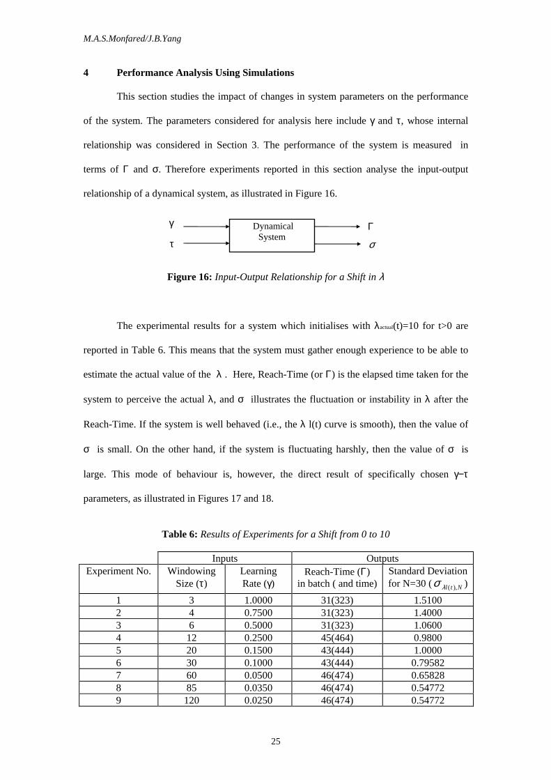
terms of Γ and σ. Therefore experiments reported in this section analyse the input-output

relationship of a dynamical system, as illustrated in Figure 16.

Figure 16: Input-Output Relationship for a Shift in λ

The experimental results for a system which initialises with λactual(t)=10 for t>0 are

reported in Table 6. This means that the system must gather enough experience to be able to

estimate the actual value of the λ . Here, Reach-Time (or Γ) is the elapsed time taken for the

system to perceive the actual λ, and σ illustrates the fluctuation or instability in λ after the

Reach-Time. If the system is well behaved (i.e., the λ l(t) curve is smooth), then the value of

σ is small. On the other hand, if the system is fluctuating harshly, then the value of σ is

large. This mode of behaviour is, however, the direct result of specifically chosen γ−τ

parameters, as illustrated in Figures 17 and 18.

Table 6: Results of Experiments for a Shift from 0 to 10

Inputs Outputs

Experiment No. Windowing Size (τ)

Learning Rate (γ)

Reach-Time (Γ) in batch ( and time)

Standard Deviation for N=30 (σ λl t N( ), )

1 3 1.0000 31(323) 1.5100 2 4 0.7500 31(323) 1.4000 3 6 0.5000 31(323) 1.0600 4 12 0.2500 45(464) 0.9800 5 20 0.1500 43(444) 1.0000 6 30 0.1000 43(444) 0.79582 7 60 0.0500 46(474) 0.65828 8 85 0.0350 46(474) 0.54772 9 120 0.0250 46(474) 0.54772

Dynamical System

γ

τ

Γ

σ


26

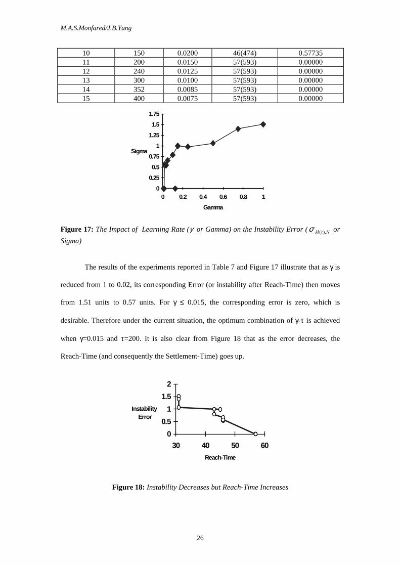
10 150 0.0200 46(474) 0.57735 11 200 0.0150 57(593) 0.00000 12 240 0.0125 57(593) 0.00000 13 300 0.0100 57(593) 0.00000 14 352 0.0085 57(593) 0.00000 15 400 0.0075 57(593) 0.00000

Gamma

Sigma

0

0.25

0.5

0.75

1

1.25

1.5

1.75

0 0.2 0.4 0.6 0.8 1

Figure 17: The Impact of Learning Rate (γ or Gamma) on the Instability Error (σ λl t N( ), or

Sigma)

The results of the experiments reported in Table 7 and Figure 17 illustrate that as γ is

reduced from 1 to 0.02, its corresponding Error (or instability after Reach-Time) then moves

from 1.51 units to 0.57 units. For γ ≤ 0.015, the corresponding error is zero, which is

desirable. Therefore under the current situation, the optimum combination of γ-τ is achieved

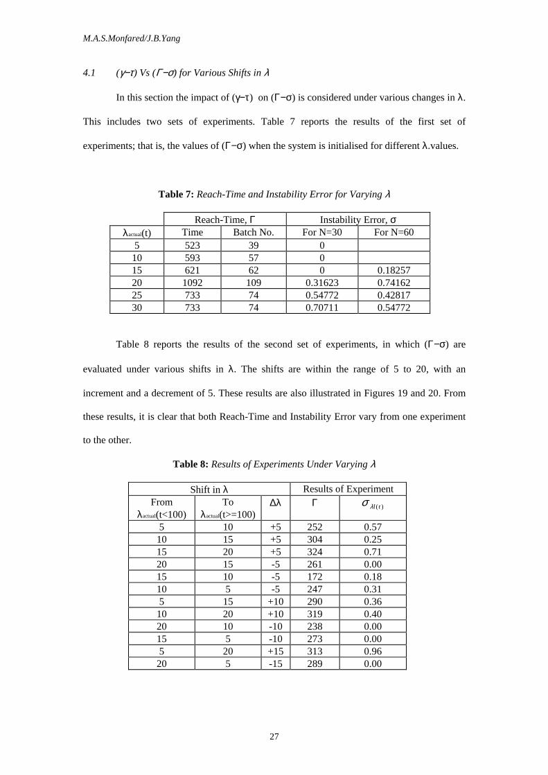
when γ=0.015 and τ=200. It is also clear from Figure 18 that as the error decreases, the

Reach-Time (and consequently the Settlement-Time) goes up.

0

0.5

1

1.5

2

30 40 50 60

Reach-Time

Instability Error

Figure 18: Instability Decreases but Reach-Time Increases


27

4.1 (γ−τ) Vs (Γ−σ) for Various Shifts in λ

In this section the impact of (γ−τ) on (Γ−σ) is considered under various changes in λ.

This includes two sets of experiments. Table 7 reports the results of the first set of

experiments; that is, the values of (Γ−σ) when the system is initialised for different λ.values.

Table 7: Reach-Time and Instability Error for Varying λ

Reach-Time, Γ Instability Error, σ λactual(t) Time Batch No. For N=30 For N=60

5 523 39 0 10 593 57 0 15 621 62 0 0.18257 20 1092 109 0.31623 0.74162 25 733 74 0.54772 0.42817 30 733 74 0.70711 0.54772

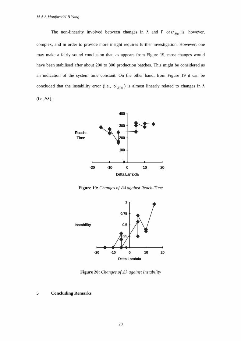
Table 8 reports the results of the second set of experiments, in which (Γ−σ) are

evaluated under various shifts in λ. The shifts are within the range of 5 to 20, with an

increment and a decrement of 5. These results are also illustrated in Figures 19 and 20. From

these results, it is clear that both Reach-Time and Instability Error vary from one experiment

to the other.

Table 8: Results of Experiments Under Varying λ

Shift in λ Results of Experiment From

λactual(t<100) To

λactual(t>=100) ∆λ Γ σ λl t( )

5 10 +5 252 0.57 10 15 +5 304 0.25 15 20 +5 324 0.71 20 15 -5 261 0.00 15 10 -5 172 0.18 10 5 -5 247 0.31 5 15 +10 290 0.36 10 20 +10 319 0.40 20 10 -10 238 0.00 15 5 -10 273 0.00 5 20 +15 313 0.96 20 5 -15 289 0.00


28

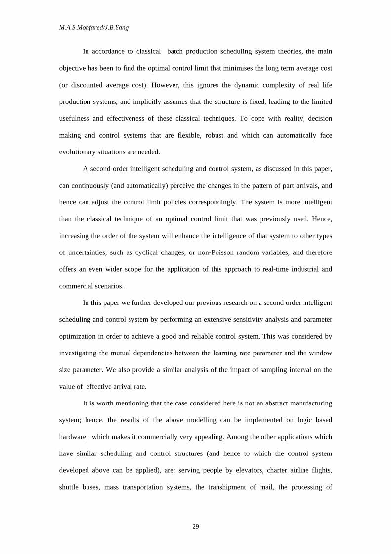
The non-linearity involved between changes in λ and Γ orσ λl t( ) is, however,

complex, and in order to provide more insight requires further investigation. However, one

may make a fairly sound conclusion that, as appears from Figure 19, most changes would

have been stabilised after about 200 to 300 production batches. This might be considered as

an indication of the system time constant. On the other hand, from Figure 19 it can be

concluded that the instability error (i.e., σ λl t( ) ) is almost linearly related to changes in λ

(i.e.,∆λ).

Delta Lambda

Reach-Time

0

100

200

300

400

-20 -10 0 10 20

Figure 19: Changes of ∆λ against Reach-Time

Delta Lambda

Instability

0

0.25

0.5

0.75

1

-20 -10 0 10 20

Figure 20: Changes of ∆λ against Instability

5 Concluding Remarks


29

In accordance to classical batch production scheduling system theories, the main

objective has been to find the optimal control limit that minimises the long term average cost

(or discounted average cost). However, this ignores the dynamic complexity of real life

production systems, and implicitly assumes that the structure is fixed, leading to the limited

usefulness and effectiveness of these classical techniques. To cope with reality, decision

making and control systems that are flexible, robust and which can automatically face

evolutionary situations are needed.

A second order intelligent scheduling and control system, as discussed in this paper,

can continuously (and automatically) perceive the changes in the pattern of part arrivals, and

hence can adjust the control limit policies correspondingly. The system is more intelligent

than the classical technique of an optimal control limit that was previously used. Hence,

increasing the order of the system will enhance the intelligence of that system to other types

of uncertainties, such as cyclical changes, or non-Poisson random variables, and therefore

offers an even wider scope for the application of this approach to real-time industrial and

commercial scenarios.

In this paper we further developed our previous research on a second order intelligent

scheduling and control system by performing an extensive sensitivity analysis and parameter

optimization in order to achieve a good and reliable control system. This was considered by

investigating the mutual dependencies between the learning rate parameter and the window

size parameter. We also provide a similar analysis of the impact of sampling interval on the

value of effective arrival rate.

It is worth mentioning that the case considered here is not an abstract manufacturing

system; hence, the results of the above modelling can be implemented on logic based

hardware, which makes it commercially very appealing. Among the other applications which

have similar scheduling and control structures (and hence to which the control system

developed above can be applied), are: serving people by elevators, charter airline flights,

shuttle buses, mass transportation systems, the transhipment of mail, the processing of


30

computer programs, the processing of job applications, the processing of library books, the

production, inventory control and shipment of commercial products, and any system where

the pattern of customer arrivals can be considered random, with non-stationary stochastic

properties (see [10], [17]) which are the subject of future research.

REFERENCES

[1] M.M. Abdelhameed, and Tolbah F.A. (2002), Design and Implementation of a Flexible

Manufacturing Control System Using Neural Network, Int. J. Flex. Manuf. Sys. 14: (3),

263-279.

[2] M.S. Akturk, and Ozkan, S. (2001), Integrated Scheduling and Tool Management in

Flexible Manufacturing Systems, Int. J. Production Research, 39: (12) 2697-2722.

[3] A. Artiba, Aghezzaf, E. H. (1997), An architecture of a multi-model system for planning

and scheduling, INT. J. COMPUTER INTEGRATED MANUFACTURING, VOL. 10,

NO. 5, 380± 393.

[4] R.G. Askin, Standridge C.R. (1993), Modelling And Analysis of Manufacturing Systems

(John Wiley & Sons).

[5] B. K. Choi, Kim, B. H. (2002), MES (manufacturing execution system) architecture for

FMS compatible to ERP (enterprise planning system), INT. J. COMPUTER

INTEGRATED MANUFACTURING, VOL. 15, NO. 3, 274–284.

[6] R.K. Deb, , Serfozo, R.F. (1973), Optimal Control of Batch Service Queues, Advances.

Appl. Probability, vol. 5, pp340-361.

[7] V. Devedzic, Radovic, D.(1999), A Framework for Building Intelligent Manufacturing

Systems IEEE Transactions on Systems, Man, and Cybernetics, Part C - Applications

and Reviews, Vol.29, No.3, August 1999, pp. 402-419.

[8] A. Hambaba (2000), Robust hybrid architecture to signals from manufacturing and

machine monitoring sensors, Journal of Intelligent and Fuzzy Systems, Vol. 9, Numbers

1-2, 29–41.

[9] T.P. Hong, Chuang, T.N. (1998), Fuzzy scheduling on two-machine flow shop Journal

of Intelligent and Fuzzy Systems, Volume 6, Number 4 ,471 – 481.


31

[10] R. Kalaputapu, Demetsky,M.J.(1995), Modeling Schedule Deviations of Buses Using

Automatic Vehicle Location Data and Artificial Neural Networks, no. 1497, July, pp 44-

52.

[11] Little, D., Rollins, R., Peck, M., and Porter, J.K. (2000), Integrated planning and

scheduling in the engineer-to-order sector, INT. J. COMPUTER INTEGRATED

MANUFACTURING, VOL. 13, NO. 6, 545–554.

[12] Lu, C. (2001), Feedback Control Real-Time Scheduling, PhD Thesis, Department of

Computer Science & Electrical Engineering, University of Virginia.

[13] K. N. Mckay, Safayeni R.R., J.A. Buzacott (1988), Job-shop shop scheduling theory:

what is relevant?, Interfaces vol. 18 , no.84, pp84-90.

[14] Mesa ( 1997), MES explained: a high level vision. White Paper 6, Manufacturing

Execution Systems Association, Pittsburgh, PA.

[15] F.H. Mitchell, Jr. (1991), CIM Systems, An Introduction to Computer-Integarted

Manufacturing, Prentice Hall.

[16] M.A.S. Monfared, , Steiner, S.J. (2000), Fuzzy Adaptive Scheduling and Control

Systems, Journal of Fuzzy Sets and Systems, No.115, pp.231-246.

[17] J. Nogami, Nakasuka, S., Tanabe, T. (1996), Real-Time Decision Support for Air Traffic

Management, Utilizing Machine Learning, Control Engineering Practice, vol. 4, no. 8,

pp 1129-1141.

[18] O. Sapena, Onaindía, E. (2002), A planning and monitoring system for dynamic

environments, Journal of Intelligent and Fuzzy Systems, Volume 12, Numbers 3-4 ,151

– 161.

[19] A. Shaout, McAuliffe, P. (2000), Fuzzy load balancing in an industrial distributed

system for job scheduling, Journal of Intelligent and Fuzzy Systems, Volume 8, Number

3, 191 – 199.

[20] F. A. Roadammer, and White, K. P.(1988), A Recent Survey of Production Scheduling,

IEEE Trans. on System, Man and Cybernetics, Vol. 18, No. 6, Nov./Dec., pp 841-851.

[21] K. Steiglitz, (1974), An Introduction to Discrete Systems, John Wiley & Sons, Inc.

[22] Tata (2002), Manufacturing Execution Systems, A Concept Note, TATA

CONSULTANCY SERVICES, India.

[23] D. Trentesaux, Pesin, P. and Tahan, C. (2000), Distributed Artificial Intelligence for

FMS Scheduling, Control and Design Support” , Journal of Intelligent Manufacturing, 11

:( 6), 573-589.

[24] J.B. Yang (2001), GA-Based Discrete Dynamic Programming Approach for Scheduling

in FMS Environments, IEEE TRANSACTIONS ON SYSTEMS, MAN, AND


32

CYBERNETICS—PART B: CYBERNETICS, VOL. 31, NO. 5, OCTOBER 2001,

pp824-835.

[25] H. J. Zimmermann (1988), Fuzzy Set Theory- and Inference Mechanism, Mathematical

Models for Decision Support, Edited by G. Mitra, NATO ASI Series, Springler-Verlag

Berlin, Heidelberg F48.

Documents

Design of an Intelligent Manufacturing Scheduling and ... Yang Journal_Papers... · Design of an Intelligent Manufacturing Scheduling and Control System Using Fuzzy Logic: Sensitivity