North Carolina Agricultural and Technical State University North Carolina Agricultural and Technical State University

Aggie Digital Collections and Scholarship Aggie Digital Collections and Scholarship

Theses Electronic Theses and Dissertations

2014

Design Of Feedback Control For Active Mass Dampers Of Excited Design Of Feedback Control For Active Mass Dampers Of Excited

Structures Structures

Sara Leona Bowen North Carolina Agricultural and Technical State University

Follow this and additional works at: https://digital.library.ncat.edu/theses

Recommended Citation Recommended Citation Bowen, Sara Leona, "Design Of Feedback Control For Active Mass Dampers Of Excited Structures" (2014). Theses. 350. https://digital.library.ncat.edu/theses/350

This Thesis is brought to you for free and open access by the Electronic Theses and Dissertations at Aggie Digital Collections and Scholarship. It has been accepted for inclusion in Theses by an authorized administrator of Aggie Digital Collections and Scholarship. For more information, please contact iyanna@ncat.edu.

Design of Feedback Control for Active Mass Dampers of Excited Structures

Sara Leona Bowen

North Carolina A&T State University

A thesis submitted to the graduate faculty

in partial fulfillment of the requirements for the degree of

MASTER OF SCIENCE

Department: Mechanical Engineering

Major: Mechanical Engineering

Major Professor: Dr. Sun Yi

Greensboro, North Carolina

2014

ii

The Graduate SchoolNorth Carolina Agricultural and Technical State University

This is to certify that the Master’s Thesis of

Sara Leona Bowen

has met the thesis requirements ofNorth Carolina Agricultural and Technical State University

Greensboro, North Carolina2014

Approved by:

Dr. Sun Yi Dr. Mannur Sundaresan

Major Professor Committee Member

Dr. Miguel Picornell-Darder Dr. Samuel Owusu-Ofori

Committee Member Department Chairperson

Dr. Sanjiv Sarin

Dean, The Graduate School

iii

c©Copyright by

Sara Leona Bowen

2014

iv

BIOGRAPHICAL SKETCH

Sara Leona Bowen was born December 5, 1989, in Greensboro, North Carolina. She

received a Bachelor of Science degree in Applied Mathematics and a minor in Physics from the

University of North Carolina Wilmington in 2012. Currently, she is a candidate for a Master of

Science degree in Mechanical Engineering at NC A&T State University.

v

DEDICATION

I dedicate this Master’s Thesis to God, who has been my provider and guidance through-

out my entire educational career. I also dedicate this work to my family and closest friends.

Without their love, support and motivational words, I would not have been able to grow into

the successful, educated woman that I am today.

vi

ACKNOWLEDGMENTS

I acknowledge and express great gratitude toward the highly acclaimed Dr. Sun Yi for

his professional guidance and support throughout my graduate studies at North Carolina A&T

State University.

vii

TABLE OF CONTENTS

LIST OF FIGURES . . . . . . . . . . . . . . . . . . . . . . . . . . . . . . . . . . . . x

LIST OF TABLES . . . . . . . . . . . . . . . . . . . . . . . . . . . . . . . . . . . . . xii

ABBREVIATIONS . . . . . . . . . . . . . . . . . . . . . . . . . . . . . . . . . . . . xiii

PHYSICAL CONSTANTS . . . . . . . . . . . . . . . . . . . . . . . . . . . . . . . . xiv

SYMBOLS . . . . . . . . . . . . . . . . . . . . . . . . . . . . . . . . . . . . . . . . . xv

ABSTRACT . . . . . . . . . . . . . . . . . . . . . . . . . . . . . . . . . . . . . . . . 1

CHAPTER 1 Introduction . . . . . . . . . . . . . . . . . . . . . . . . . . . . . . . 2

1.1 Motivation . . . . . . . . . . . . . . . . . . . . . . . . . . . . . . . . . . . . . 2

1.2 Solution and Concerns . . . . . . . . . . . . . . . . . . . . . . . . . . . . . . 4

1.3 Application . . . . . . . . . . . . . . . . . . . . . . . . . . . . . . . . . . . . 4

CHAPTER 2 Literature Review . . . . . . . . . . . . . . . . . . . . . . . . . . . . 6

2.1 Supplementary Damping Systems . . . . . . . . . . . . . . . . . . . . . . . . 6

2.2 Mass Damping Systems . . . . . . . . . . . . . . . . . . . . . . . . . . . . . . 7

2.3 Controller Design . . . . . . . . . . . . . . . . . . . . . . . . . . . . . . . . . 8

2.3.1 Eigenvalue Assignment . . . . . . . . . . . . . . . . . . . . . . . . . . 9

2.3.2 Linear Quadratic Regulator . . . . . . . . . . . . . . . . . . . . . . . . 11

2.3.3 Model Predictive Control . . . . . . . . . . . . . . . . . . . . . . . . . 13

2.3.4 Adaptive Control . . . . . . . . . . . . . . . . . . . . . . . . . . . . . 14

CHAPTER 3 Modeling . . . . . . . . . . . . . . . . . . . . . . . . . . . . . . . . . 16

3.1 AMD-1 Schematic and Design Specifications . . . . . . . . . . . . . . . . . . 16

3.2 Equation of Motion . . . . . . . . . . . . . . . . . . . . . . . . . . . . . . . . 17

3.2.1 Free Body Diagram . . . . . . . . . . . . . . . . . . . . . . . . . . . . 17

viii

3.2.2 Lagrange’s Method . . . . . . . . . . . . . . . . . . . . . . . . . . . . 20

CHAPTER 4 Simulation . . . . . . . . . . . . . . . . . . . . . . . . . . . . . . . . 24

4.1 MATLAB Simulations . . . . . . . . . . . . . . . . . . . . . . . . . . . . . . 25

4.1.1 Controllability and Observability . . . . . . . . . . . . . . . . . . . . . 26

4.1.2 State-Feedback Design . . . . . . . . . . . . . . . . . . . . . . . . . . 27

4.1.3 Full-Order State Observer Design . . . . . . . . . . . . . . . . . . . . 31

4.2 Simulink Simulations . . . . . . . . . . . . . . . . . . . . . . . . . . . . . . . 33

4.2.1 Open-Loop . . . . . . . . . . . . . . . . . . . . . . . . . . . . . . . . 33

4.2.2 Closed-Loop - Feedback Controller . . . . . . . . . . . . . . . . . . . 33

4.2.3 Closed-Loop - Feedback Controller with an Observer . . . . . . . . . . 34

CHAPTER 5 Parameter Estimation . . . . . . . . . . . . . . . . . . . . . . . . . . 38

5.1 Simulink Toolbox . . . . . . . . . . . . . . . . . . . . . . . . . . . . . . . . . 38

5.1.1 External Sensor Tests . . . . . . . . . . . . . . . . . . . . . . . . . . . 39

CHAPTER 6 Results . . . . . . . . . . . . . . . . . . . . . . . . . . . . . . . . . . . 43

6.1 Experimental Testing . . . . . . . . . . . . . . . . . . . . . . . . . . . . . . . 43

6.2 Estimated vs. Original Parameter Tests . . . . . . . . . . . . . . . . . . . . . . 44

6.3 Eigenvalue Assignment Results . . . . . . . . . . . . . . . . . . . . . . . . . . 45

6.4 Linear Quadratic Regulation . . . . . . . . . . . . . . . . . . . . . . . . . . . 56

CHAPTER 7 Conclusion . . . . . . . . . . . . . . . . . . . . . . . . . . . . . . . . 59

7.1 Discussion . . . . . . . . . . . . . . . . . . . . . . . . . . . . . . . . . . . . . 59

7.2 Future Research . . . . . . . . . . . . . . . . . . . . . . . . . . . . . . . . . . 60

REFERENCES . . . . . . . . . . . . . . . . . . . . . . . . . . . . . . . . . . . . . . . 62

APPENDIX A MATLAB Script for Simulating the AMD . . . . . . . . . . . . . . 67

APPENDIX B MATLAB Script for Eigenvalue Assignement . . . . . . . . . . . . . 70

ix

APPENDIX C MATLAB Script for LQR . . . . . . . . . . . . . . . . . . . . . . . . 72

APPENDIX D Simulink Diagrams . . . . . . . . . . . . . . . . . . . . . . . . . . . 74

D.1 State Observer . . . . . . . . . . . . . . . . . . . . . . . . . . . . . . . . . . . 74

D.2 Quanser AMD-1 plant with External QUARC CONTROL . . . . . . . . . . . 75

x

LIST OF FIGURES

1.1 Leading natural disasters by overall economic loss and human fatality, since 1980 [22]. 2

1.2 Global heat-map of active earthquake zones (green, yellow, red zones) and nuclear

power plant locations (purple dots) [26]. . . . . . . . . . . . . . . . . . . . . . . . 3

3.1 Experimental setup. . . . . . . . . . . . . . . . . . . . . . . . . . . . . . . . . . 16

3.2 AMD-1 free body diagram without structure viscous damping. . . . . . . . . . . . . 18

3.3 AMD-1 free body diagram with structure viscous damping. . . . . . . . . . . . . . . 19

4.1 The system’s natural step response (top) and impulse response (bottom). . . . . . . . 26

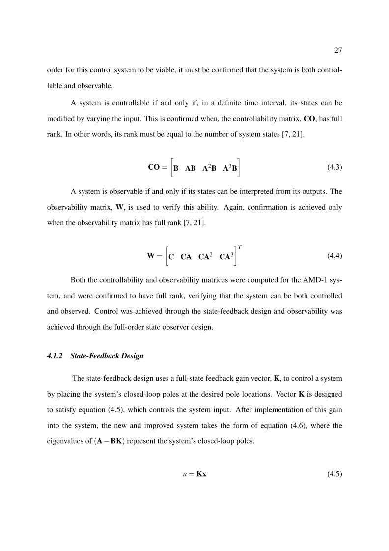
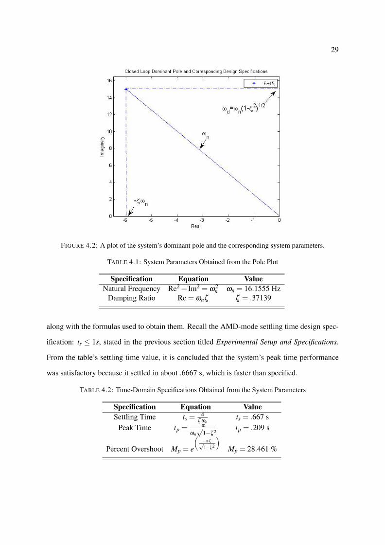
4.2 A plot of the system’s dominant pole and the corresponding system parameters. . . . . 29

4.3 The system’s controlled step response (top) and impulse response (bottom). . . . . . . 30

4.4 Open-loop Simulink diagram. . . . . . . . . . . . . . . . . . . . . . . . . . . . . 33

4.5 Open-loop scope of the system’s response. . . . . . . . . . . . . . . . . . . . . . . 34

4.6 Closed-loop Simulink diagram. . . . . . . . . . . . . . . . . . . . . . . . . . . . 34

4.7 Closed-loop scope of the system’s response. . . . . . . . . . . . . . . . . . . . 35

4.8 State observer Simulink - a comparison of the plant’s and observer plant’s state responses. 36

4.9 State observer Simulink - a comparison of the plant’s and observer plant’s output re-

sponses. . . . . . . . . . . . . . . . . . . . . . . . . . . . . . . . . . . . . . . 36

4.10 State observer Simulink - system’s error. . . . . . . . . . . . . . . . . . . . . . . . 37

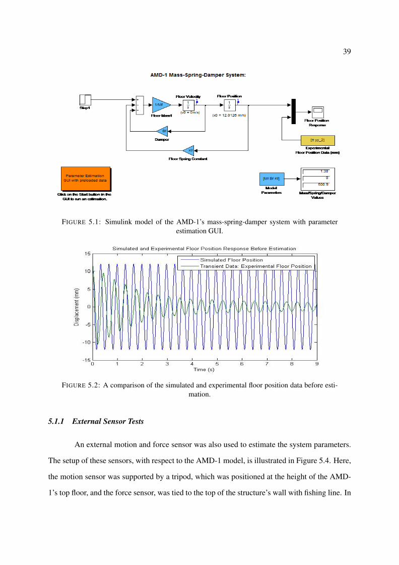
5.1 Simulink model of the AMD-1’s mass-spring-damper system with parameter

estimation GUI. . . . . . . . . . . . . . . . . . . . . . . . . . . . . . . . . . . 39

5.2 A comparison of the simulated and experimental floor position data before es-

timation. . . . . . . . . . . . . . . . . . . . . . . . . . . . . . . . . . . . . . . 39

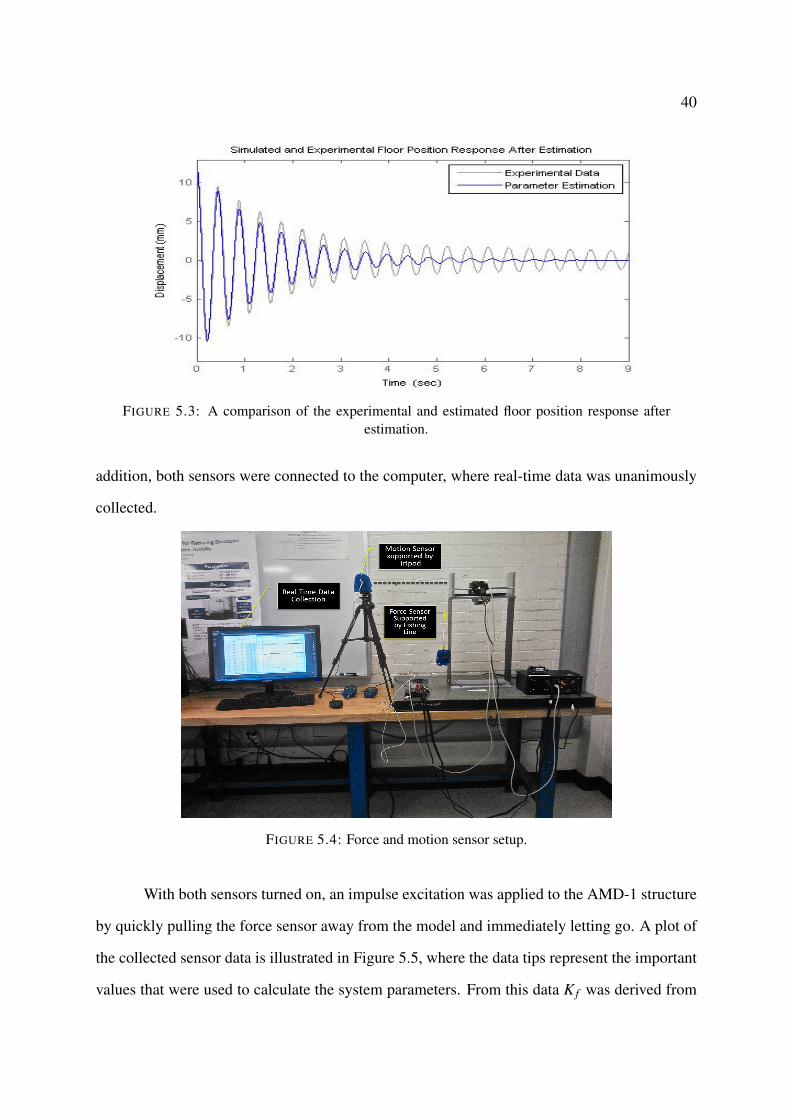
5.3 A comparison of the experimental and estimated floor position response after

estimation. . . . . . . . . . . . . . . . . . . . . . . . . . . . . . . . . . . . . . 40

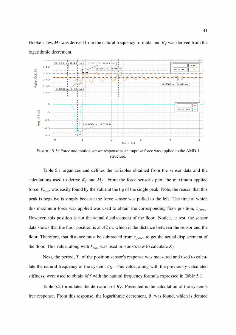
5.4 Force and motion sensor setup. . . . . . . . . . . . . . . . . . . . . . . . . . . 40

xi

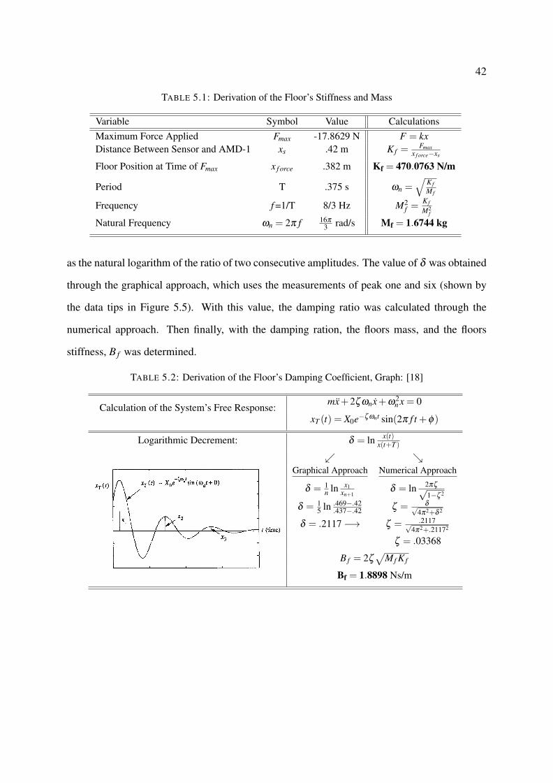
5.5 Force and motion sensor response as an impulse force was applied to the AMD-

1 structure. . . . . . . . . . . . . . . . . . . . . . . . . . . . . . . . . . . . . . 41

6.1 Floor position and acceleration, cart position, and cart motor voltage responses. 44

6.2 A comparison of the floor position (left) and cart motor voltage (right) data

obtained from the original vs. estimated parameters. . . . . . . . . . . . . . . . 45

6.3 A plot of the exponential function provided by the closed-loop poles. . . . . . . 46

6.4 Location of the poles considered for the eigenvalue assignment tests. . . . . . . 47

6.5 Eigenvalue Assignment Results: Simulated and experimental floor acceleration

peak trends, for both parameter tests. . . . . . . . . . . . . . . . . . . . . . . . 49

6.6 Eigenvalue Assignment Results: Simulated and experimental floor acceleration

RMS trends, for both parameter tests. . . . . . . . . . . . . . . . . . . . . . . . 50

6.7 Eigenvalue Assignment Results: Original parameter floor acceleration responses,

produced when the controller’s dominant pole locations were at −3 and −6. . . 51

6.8 Eigenvalue Assignment Results: Sensor parameter floor acceleration responses,

produced when the controller’s dominant pole locations were at −3 and −6. . . 51

6.9 Eigenvalue Assignment Results: Voltage peak trends. . . . . . . . . . . . . . . 53

6.10 Eigenvalue Assignment Results: Voltage RMS trends. . . . . . . . . . . . . . . 55

6.11 Eigenvalue Assignment Results: Filtered floor acceleration RMS trends. . . . . 55

6.12 LQR results: Filterend floor acceleration RMS trends. . . . . . . . . . . . . . . 58

6.13 LQR results: Voltage RMS trends. . . . . . . . . . . . . . . . . . . . . . . . . 58

D.1 State observer Simulink diagram. . . . . . . . . . . . . . . . . . . . . . . . . . 74

D.2 Simulink model of the active control design for seismically excited Nuclear

Power Plants [29]. . . . . . . . . . . . . . . . . . . . . . . . . . . . . . . . . . 75

xii

LIST OF TABLES

1.1 Leading Natural Disaster Deaths, Since 1980 [22] . . . . . . . . . . . . . . . . 3

1.2 Countries with the Most Nuclear Power Plant Locations [1, 26, 27] . . . . . . . 3

4.1 System Parameters Obtained from the Pole Plot . . . . . . . . . . . . . . . . . 29

4.2 Time-Domain Specifications Obtained from the System Parameters . . . . . . . 29

5.1 Derivation of the Floor’s Stiffness and Mass . . . . . . . . . . . . . . . . . . . 42

5.2 Derivation of the Floor’s Damping Coefficient, Graph: [18] . . . . . . . . . . . 42

6.1 The Sets of System Parameters Values Used for Testing . . . . . . . . . . . . . 44

6.2 RMS Values of the Original and Estimated Parameter Test Responses . . . . . . 45

6.3 Eigenvalue Assignment Results: Experimental and Simulated Floor Accelera-

tion Peak and RMS Data . . . . . . . . . . . . . . . . . . . . . . . . . . . . . 48

6.4 Eigenvalue Assignment Results: Floor Position Peak Ratio Data From Both

Parameter Tests . . . . . . . . . . . . . . . . . . . . . . . . . . . . . . . . . . 52

6.5 Eigenvalue Assignment Results: Experimental Voltage and Filtered Floor Ac-

celeration Peak Data . . . . . . . . . . . . . . . . . . . . . . . . . . . . . . . . 52

6.6 Eigenvalue Assignment Results: Experimental Filtered Floor Acceleration RMS

Data . . . . . . . . . . . . . . . . . . . . . . . . . . . . . . . . . . . . . . . . 54

6.7 LQR Results: Experimental Filtered Floor Acceleration RMS Data . . . . . . . 57

6.8 LQR Results: Experimental Voltage RMS Data . . . . . . . . . . . . . . . . . 57

xiii

ABBREVIATIONS

AMD-1 Active Mass Damper - One Floor

AR Auto-regressive

AWS Active Wireless Sensing

DOF Degree(s)-Of-Freedom

EMF ElectroMotive-Force

EOM Equation of Motion

FB Feedback

FF Feedforward

LSS Large Space Structures

LQR Linear Quadratic Regulation

MDS Mass Damper System

MIMO Multi-Input and Multi-Output

MPC Model Predictive Control

PEA Partial Eigenvalue Analysis

PID Proportional-Integrated-Derivative

PV Proportional-Velocity

RMS Root Mean Square

SDS Supplementary Damping Systems

SISO Single-Input and Single-Output

TLCD Tuned Liquid Column Damper

TMD Tuned Mass Damper

TSD Tuned Sloshing Damper

Y-W Yule-Walker

xiv

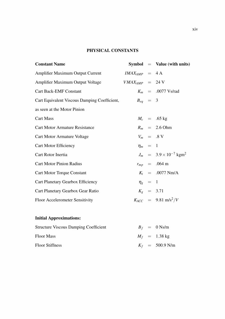
PHYSICAL CONSTANTS

Constant Name Symbol = Value (with units)

Amplifier Maximum Output Current IMAXAMP = 4 A

Amplifier Maximum Output Voltage V MAXAMP = 24 V

Cart Back-EMF Constant Km = .0077 Vs/rad

Cart Equivalent Viscous Damping Coefficient, Beq = 3

as seen at the Motor Pinion

Cart Mass Mc = .65 kg

Cart Motor Armature Resistance Rm = 2.6 Ohm

Cart Motor Armature Voltage Vm = .8 V

Cart Motor Efficiency ηm = 1

Cart Rotor Inertia Jm = 3.9×10−7 kgm2

Cart Motor Pinion Radius rmp = .064 m

Cart Motor Torque Constant Kt = .0077 Nm/A

Cart Planetary Gearbox Efficiency ηg = 1

Cart Planetary Gearbox Gear Ratio Kg = 3.71

Floor Accelerometer Sensitivity KACC = 9.81 m/s2/V

Initial Approximations:

Structure Viscous Damping Coefficient B f = 0 Ns/m

Floor Mass M f = 1.38 kg

Floor Stiffness K f = 500.9 N/m

xv

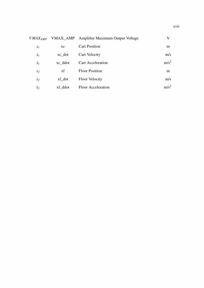
SYMBOLS

Symbol MATLAB Description Unit

J Cost Function

L Lagrangian J

Mp Percent Overshoot %

Qxc Generalized Force, N

Applied on the Generalized Coordinate xc

Qx f Generalized Force, N

Applied on the Generalized Coordinate x f

s Laplace Operator

tp Peak Time s

ts Settling Time s

Ttc Cart Translational Kinetic Energy J

Trc Cart Rotor Rotational Kinetic Energy J

Tt f Floor Translational Kinetic Energy J

TT Total Kinetic Energy of the AMD-1 System J

VT Total Potential Energy of the AMD-1 System J

A A System Matrix

B B Input Matrix

C C Output Matrix

CO CO Controllability Matrix

D D Input-Output Matrix

G G Full-Order State Observer Gain Matrix

K K Full-State Feedback Gain Vector

OP OP Closed-Loop Pole Vector,

xvi

due to the Observer Error Dynamics

P P Closed-Loop Pole Vector,

due to the State Feedback Law

W W Observability Matrix

X X Actual State Vector

X0 X0 Estimated State Vector

Y Y Actual Output Vector

Y0 Y0 Estimated Output Vector

B f Bf Structure Viscous Damping Coefficient Ns/m

Beq Beq Cart Equivalent Viscous Damping Coefficient,

as seen at the Motor Pinion

Fc Fc Cart Driving Force (produced by the DC motor) N

IMAXAMP IMAX_AMP Amplifier Maximum Output Current A

KACC K_ACC Floor Accelerometer Sensitivity m/s2/V

K f Kf Floor Stiffness N/m

Kg Kg Cart Planetary Gearbox Gear Ratio

Km Km Cart Back-EMF Constant V

Kt Kt Cart Motor Torque Constant Nm

Jm Jm Cart Rotor Inertia kgm2

Mc Mc Cart Mass kg

M f Mf Floor Mass kg

ηg Eff_g Cart Planetary Gearbox Efficiency

ηm Eff_m Cart Motor Efficiency

Rm Rm Cart Motor Resistance Ohm

rmp r_mp Cart Motor Pinion Radius mm

Vm Vm Cart Motor Voltage V

xvii

V MAXAMP VMAX_AMP Amplifier Maximum Output Voltage V

xc xc Cart Position m

xc xc_dot Cart Velocity m/s

xc xc_ddot Cart Acceleration m/s2

x f xf Floor Position m

x f xf_dot Floor Velocity m/s

x f xf_ddot Floor Acceleration m/s2

1

ABSTRACT

Annually, our world experiences thousands of seismic events that are the cause of hun-

dreds of structural disasters and human fatalities. The objective of the presented research is to

contribute to the world’s social, economic, and environmental needs by designing an optimized

feedback control for active mass dampers (AMDs) by reducing oscillations. The optimal de-

sign will meet the required specifications and maintain a structure’s quasi-ideal, static position

throughout a seismic event. The system’s equation of motion (EOM) is derived by using the

Lagrangian Method and the free-body diagram. All the simulated and experimental responses

of the AMD-1 system are obtained using MATLAB and Simulink. The experimental data is

collected from various tests performed on a single-story building model. The techniques uti-

lized for improvement of the AMD’s feedback control include parameter estimation, eigenvalue

assignment, and linear quadratic regulation (LQR). As success is achieved with the AMD feed-

back control, future research can focus on idealizing the AMD’s performance in a system with

multiple degrees of freedom.

2

CHAPTER 1

INTRODUCTION

1.1 Motivation

Annually, our world experiences thousands of natural disasters (seismic events) that

are the cause of hundreds of structural disasters and human fatalities. These disasters can

be the effect of high wind speeds or an excitation of the Earth’s crust. A map of the global

economic effect of leading natural disasters, since 1980, is portrayed in Figure 1.1 [22]. This

map recognizes China, Japan, United States, Thailand, Chile and the Caribbean Islands as the

primary world victims of natural disasters, and they are ranked in the order of most to least

number of casualties. The summed number of deaths, caused by each natural disaster, and

their percentages are organized into Table 1.1, where it clearly shows that earthquakes are the

leading cause of the world’s natural disaster related deaths.

FIGURE 1.1: Leading natural disasters by overall economic loss and human fatality,since 1980 [22].

With respect to structural disasters, earthquakes have a growing negative impact on

nuclear power plants. Figure 1.2 illustrates the worldwide location of both active earthquake

3

zones, based on the seismic data gathered from the United States Geological Survey, and nu-

clear power plants, based on the nuclear power station information gathered from the Interna-

tional Atomic Energy Agency [1, 26, 27]. The number of plants and the overall percentages of

the top five countries, home to the most amount of nuclear power plants in the world, are listed

in Table 1.2. It is observed that two of the top three natural disaster victims (United States and

Japan) are collectively home to over 35% of the world’s nuclear power plants. This leads to a

higher potential risk for social, economic, and environmental loss, particularly, but not limited

to, the United States and Japanese areas.

FIGURE 1.2: Global heat-map of active earthquake zones (green, yellow, red zones) and nu-clear power plant locations (purple dots) [26].

TABLE 1.1: Leading Natural DisasterDeaths, Since 1980 [22]

Earth Water WindEarthquakes Tsunamis & Floods Hurricanes

106,897 22,654 1,492

81.57 % 17.29 % 1.14 %

TABLE 1.2: Countries with the MostNuclear Power Plant Locations [1, 26, 27]

Country Plants Worldly %United States 79 31.73 %Germany 26 10.44 %France 22 8.84 %Japan 19 7.63 %United Kingdom 17 6.83 %

Total Plants 249 65.47 %

4

1.2 Solution and Concerns

A potential solution to this problem includes the installation of active mass dampers

(AMDs) into the buildings and plants at risk. In the 1980’s, researchers began considering the

use of AMDs to achieve structural control [38]. Yet in 2011, thirty years later, it was still rare

to hear about any such installations [32]. This hesitation, to commercially utilize AMDs, could

have been the result of several different limitations and concerns. When modeling large space

structures (LSS), the dynamics of the AMD system are nonlinear, and non-linearity can lead

to mathematical complexity and uncertainty. Unfortunately, the AWS (active wireless sensing)

units, used in wireless AMDs, have limited computational abilities that stem from the limited

availability of voltage, money, and resources. Consider the design of feedback controllers in

a MIMO (multi-input and multi-output) system, they require a vast amount of input voltage,

resulting in extremely high expenses. For this reason, restrictions must be put on the design

of the feedback control. These design specifications are made to decrease the effect of these

complications and lead to the design of a light weight device with a low power demand, a low

energy consumption rate, and the utilization a robust control scheme [3, 13, 32, 33, 38].

1.3 Application

The development and implementation of the feedback control design specifications

lead to an increased usage of AMDs. As of last year (2013), AMDs had been installed in fifty

Japanese buildings, one of which was a twenty four-story building in Tokyo, which survived the

2011 typhoon and earthquake. The AMD’s performance was closely monitored, and the results

suggested the AMD’s control performance and energy regeneration efforts were successful.

Analysis of this data provided evidence that the regeneration system saved as much as 35-65%

of the energy that the AMD was predicted to have consumed without it. Verification of this

success is presented in [39].

5

The objective of the presented research is to further contribute to the World’s social,

economic, and environmental needs by designing an ideal feedback control for AMDs. It is in-

tended that the optimized design will meet the required specifications and maintain a structure’s

quasi-ideal, static position throughout a seismic event. The system used in this work is a one

story building model with an installed AMD (AMD-1). To design the feedback control, the sys-

tem’s equation of motion (EOM) is derived by using the Lagrangian Method and the free body

diagram. Simulated and experimental AMD-1 responses are obtained from a variety of tests

using MATLAB and Simulink. The techniques used for improvement of the AMD’s feedback

control include parameter estimation, eigenvalue assignment, and linear quadratic regulation

(LQR). As success is achieved with the AMD feedback control, future research can focus on

idealizing the AMD’s performance in a MIMO system.

6

CHAPTER 2

LITERATURE REVIEW

Exceptional progress has been made in the field of system dynamics with respect to

structural control. Structural design techniques have evolved over the years to help structures

withstand seismic events and ensure safety to those in and around the structure. The use of

various supplementary damping systems (SDS) and mass damping systems (MDS) have been

widely studied and tested on structures susceptible to seismic excitation. Within these damping

systems, lies a controller that is used to increase the decay rate of the system. Depending

on the characteristics of the system-to-be-controlled, these controllers have the potential to be

highly complex and demand an intricate design. This section provides a brief background and

description for a variety of damping systems and controller design techniques.

2.1 Supplementary Damping Systems

A Supplementary Damping System (SDS) is a control system that is designed to absorb

structure vibrations [30]. Three of the main types of SDS are passive, semi-active, and active

control systems. Passive control is the simplest and cheapest form of an SDS. This type of

system uses mechanical control forces to oppose the motion of the structure, and requires no

external power. Consequently, its performance is always reliable, even in the event of a power

outage. The downfall is, a passive system is unable to adapt to the fluctuation of the system’s

parameters (mass, damping coefficient and stiffness) over time.

In a semi-active SDS, the system’s parameters can be modified to update the control

system. Control is achieved by counteracting the structure’s motion with controlled resis-

tive forces, which requires a small amount of external power. Since the system utilizes the

structure’s motion to develop these control forces, stability is always guaranteed; however, the

7

performance is limited. It achieves the highest efficiency in situations where the dynamic char-

acteristics and excitation conditions are well known.

Active control systems are the more modern form of control systems and are found to

be the most versatile. They possess the ability to both add and dissipate energy in the system

by the use of force generators. These generators have a high demand for power, which can lead

to high expenses, and if the system were to go into an out-of-control state, it can increase the

potential for system destabilization [17, 30]. Despite these concerns, an active control system

was chosen to be used in this study because it has the highest potential for increased success.

2.2 Mass Damping Systems

Mass damper systems (MDS) are specific types of SDSs that use the the weight of a

mass to dissipate the energy transferred to the structure by a seismic event. The most effective

location for such systems is at or near the area where the vibration is at the highest amplitude.

Typically, this is at the top or bottom of a structure, or at the outermost point of an overhang.

The four most popular types of dampers used in these systems are tuned liquid column dampers,

tuned sloshing dampers, tuned mass dampers, and active mass dampers [30].

Tuned liquid column dampers (TLCD) are one of the cheapest in cost. They use the

mass and motion of a liquid, stored in a U-shaped tank, to counteract the vibration of a struc-

ture. Further energy dissipation can be achieved simply by installing adjustable gates. The

Bernoulli’s equation is used to derive this system’s dynamics, and is shown to only achieve

effectiveness in one axis [11].

Tuned sloshing dampers (TSD) use the surface waves of a liquid to absorb a structure’s

vibration. The tank, used to hold the liquid, is specifically engineered so that the frequency of

the liquid’s surface wave matches the natural frequency of the structure. Similar to the TLCD,

the tank also incorporates baffles to further dissipate energy, but effectiveness can be achieved

in two orthogonal axes, simultaneously, when a rectangular tank is used [30].

8

Tuned Mass Dampers (TMD) use a mass (typically steel or concrete) suspended on

cables to counteract the force on a structure. In situations were minimum height requirements

become a variable in the problem, two masses, suspended by a combination of cables and struts,

are used. TMDs are tuned to be effective in two axes, simultaneously, and they incorporate

hydraulic cylinders to dissipate energy [20, 30].

Active Mass Dampers (AMD) are similar to TMDs, but they stabilize the system by

utilizing a driving mechanism instead of energy dissipators. Typically hydraulic actuators, with

their high durability and high cost performance rating, are used to drive the system, and are

based on the structure’s motion sensor input. The driving mechanism is controlled by a com-

puter, and therefore requires power, but it allows the control system to react to the structure’s

motion in real time [38]. It is For this reason that an AMD was chosen to be used in this study.

2.3 Controller Design

Within the AMD of this study’s active control system, there exists a controller. The

design of this controller must be unique to the provided system. Research suggests that the

most popular controller design methods include the eigenvalue assignment method and linear

quadratic regulator (LQR) design. Some newer controller design methods that have been uti-

lized in other studies include model predictive control (MPC) and adaptive control. It was

decided that the newness of these control methods imply there is still much to be learned about

them and they lack in reliability. For that reason, only the eigenvalue assignment method and

LQR design will be used in this study. Nonetheless, a brief background and description for

each of these controller design techniques is provided in this section for enlightening purposes.

9

2.3.1 Eigenvalue Assignment

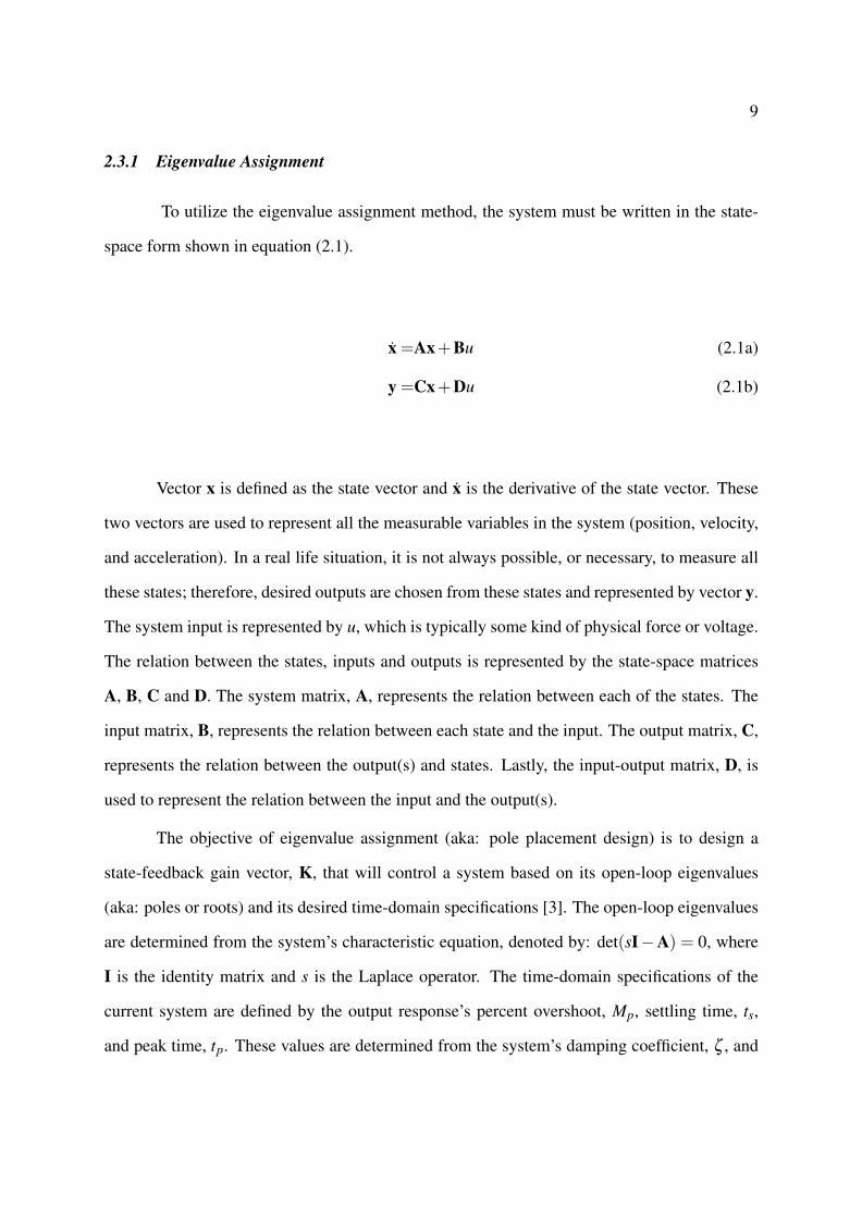
To utilize the eigenvalue assignment method, the system must be written in the state-

space form shown in equation (2.1).

x =Ax+Bu (2.1a)

y =Cx+Du (2.1b)

Vector x is defined as the state vector and x is the derivative of the state vector. These

two vectors are used to represent all the measurable variables in the system (position, velocity,

and acceleration). In a real life situation, it is not always possible, or necessary, to measure all

these states; therefore, desired outputs are chosen from these states and represented by vector y.

The system input is represented by u, which is typically some kind of physical force or voltage.

The relation between the states, inputs and outputs is represented by the state-space matrices

A, B, C and D. The system matrix, A, represents the relation between each of the states. The

input matrix, B, represents the relation between each state and the input. The output matrix, C,

represents the relation between the output(s) and states. Lastly, the input-output matrix, D, is

used to represent the relation between the input and the output(s).

The objective of eigenvalue assignment (aka: pole placement design) is to design a

state-feedback gain vector, K, that will control a system based on its open-loop eigenvalues

(aka: poles or roots) and its desired time-domain specifications [3]. The open-loop eigenvalues

are determined from the system’s characteristic equation, denoted by: det(sI−A) = 0, where

I is the identity matrix and s is the Laplace operator. The time-domain specifications of the

current system are defined by the output response’s percent overshoot, Mp, settling time, ts,

and peak time, tp. These values are determined from the system’s damping coefficient, ζ , and

10

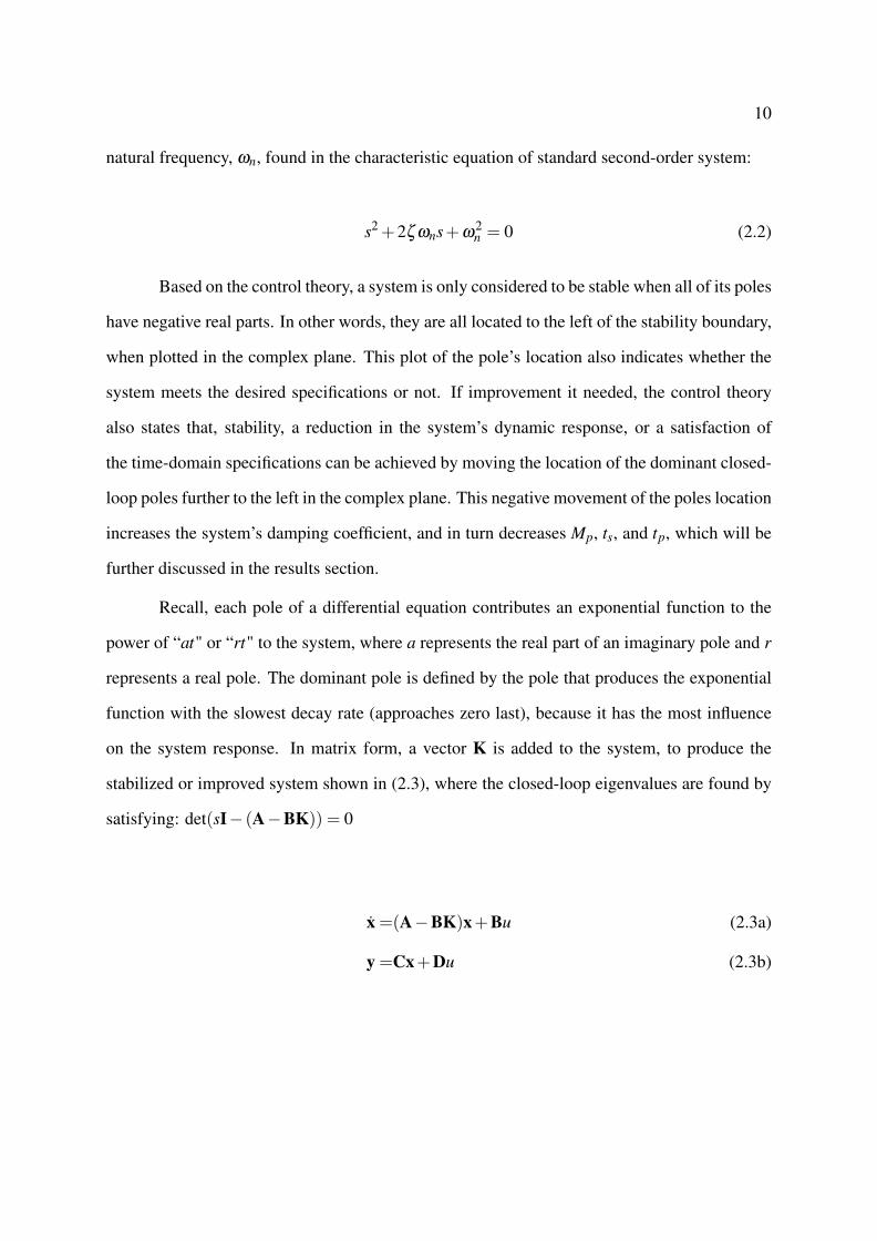
natural frequency, ωn, found in the characteristic equation of standard second-order system:

s2 +2ζ ωns+ω2n = 0 (2.2)

Based on the control theory, a system is only considered to be stable when all of its poles

have negative real parts. In other words, they are all located to the left of the stability boundary,

when plotted in the complex plane. This plot of the pole’s location also indicates whether the

system meets the desired specifications or not. If improvement it needed, the control theory

also states that, stability, a reduction in the system’s dynamic response, or a satisfaction of

the time-domain specifications can be achieved by moving the location of the dominant closed-

loop poles further to the left in the complex plane. This negative movement of the poles location

increases the system’s damping coefficient, and in turn decreases Mp, ts, and tp, which will be

further discussed in the results section.

Recall, each pole of a differential equation contributes an exponential function to the

power of “at" or “rt" to the system, where a represents the real part of an imaginary pole and r

represents a real pole. The dominant pole is defined by the pole that produces the exponential

function with the slowest decay rate (approaches zero last), because it has the most influence

on the system response. In matrix form, a vector K is added to the system, to produce the

stabilized or improved system shown in (2.3), where the closed-loop eigenvalues are found by

satisfying: det(sI− (A−BK)) = 0

x =(A−BK)x+Bu (2.3a)

y =Cx+Du (2.3b)

11

Since this world is imperfect, moving the poles too far to the left will cause discrep-

ancies. For this reason, it is important to determine and understand the limitations unique to

each system. For example, active control has the potential to introduce time delays in the con-

trol effort’s FB loop, and a MIMO system has a higher risk of asymptotic stability when using

low-gain controllers [2, 3, 5, 8, 9, 12, 28, 34].

Some of the newest background on the eigenvalue assignment method includes the ad-

dressing of the issue regarding the degrading performance in controllers, for systems with time

variant parameters, in 2007. This solution involved the utilization of eigenvalue assignment

techniques to stabilize the system with both, robust and adaptive controllers. It was found

that the robust pole placement controllers required lower actuator voltages than the adaptive

pole placement controllers. But it was also found that the adaptive controllers were found to

be noise tolerant, while the robust controllers were found to be noise sensitive. Furthermore,

studies show that robust stability and performance can only be achieved for a select range of

parameter uncertainties [14].

More recently, in 2011, a modified version of the eigenvalue assignment method was

discussed, and referred to as partial eigenvalue analysis (PEA). In PEA, only a selection of

the open-loop eigenvalues are modified in the FB controller. PEA was found to be effective

because it can keep a structure safely active under excitation, with minimal control effort [4, 8].

2.3.2 Linear Quadratic Regulator

In 2005, three numerical design techniques, used for optimizing active structural con-

trol during seismic activity, were presented. These techniques include LQR, discrete time-

dependent non-integral LQR, and generalized LQR. Reseach suggests that When designing an

LQR system, it should be taken into consideration that they require multiple sensors, integrat-

ing amplifiers and cables to achieve vibration control. However, it is also suggested that by

utilizing vibration control techniques that apply the robust control theory, the required equip-

ment may be minimized [36]. Nonetheless, this issue was not presented in the work of this

12

thesis.

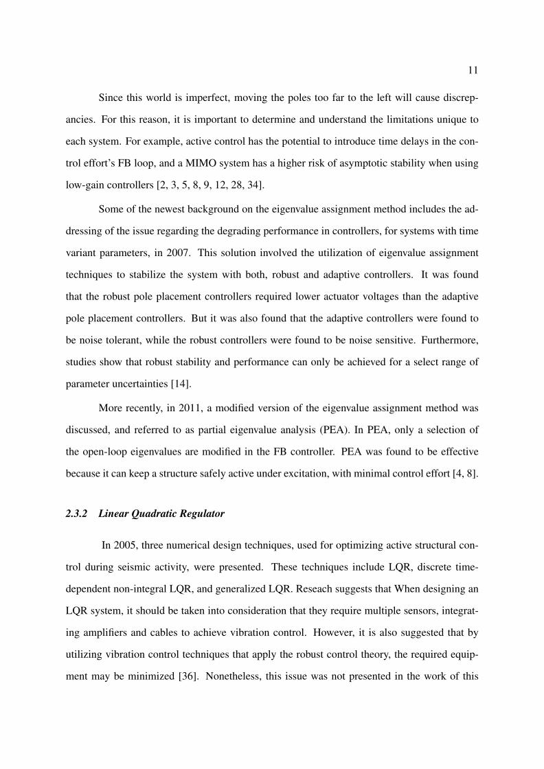
The objective of the LQR method is to obtain a control force, u : [0,T ]→ Rm, that

is proportional to the structural response and that minimizes the cost function, J [25]. This

is achieved by utilizing an integral performance index and selecting the appropriate feedback

gains and full-state observers, based on the input and output weight matrices [5, 10, 19, 35].

The cost function, for a continuous time system, is expressed by equation (2.4), where

R represents the input weight matrix and Q represents the output weight matrix.

J(u) =∫

∞

0

(xT Qx+uT Ru

)dt (2.4)

Given the system dynamics are described by equation (2.5), where x is the state vector, x is the

derivative of the state vector, A is the system matrix, and B is the input matrix.

x = Ax+Bu (2.5)

J gets minimized by the state feedback law, u = −kx. The minimized function returns the

solution, S, of the Riccati equation (2.6), and the closed loop poles, the determinant of (A−BK)

[5, 25].

AT S+SA−SBR−1BT S+Q = 0 (2.6)

Finally, the feedback gain vector, K, is derived from S by the use of the following expression:

K = R−1BT S (2.7)

The limitations of the LQR method include [25]:

• (A,B) must be stabilizable.

• R > 0 and definite.

13

• Q≥ 0 and semi-definite.

• (Q,A) must have no unobservable mode on the imaginary axis.

The discrete time-dependent non-integral LQR method is exactly the same as the LQR

method, but it is for a discrete-time state-space model. The discrete feedback control law,

u[n] = ˘Kx[n], minimizes the discrete cost function (2.8), given the system dynamics (2.9).

Since it is discrete, this method must reach optimality at every time instant and is used when

the control forces are set to be proportional to both, the structural response and the time step

[19, 25].

J =∞

∑n=0{xT Qx+uT Ru} (2.8)

x[n+1] = Ax[n]+Bu[n] (2.9)

Lastly, the generalized LQR, is simply defined as a generalization of the criteria from

both the LQR and the discrete time-dependent non-integral LQR [19].

2.3.3 Model Predictive Control

In 2001, a general formulation of the (MPC) scheme was introduced by Mei and et al.

The objective is to minimize both the trajectory deviation between the predicted and desired

responses as well as the control effort subjected to specific constraints. This is achieved by

using a prediction model of the system response, formulated using both feedforward (FF) and

feedback (FB) loops, to control the real-time response of a seismically excited structure. [23].

To obtain the FF loop, two types of inputs were used: the Kanai-Tajimi Type model

and an Auto-Regressive (AR) model. The Kanai-Tajimi model simulates an earthquake input

based on the concept of a random pulse train. It also possesses the potential to incorporate the

14

propagation, reflection, and refraction of seismic waves as they travel through the ground [16].

The Auto-Regressive model simulates the ground motion of an earthquake with a real-time

FF loop. It is constantly updated with real-time, on-line observations, which guarantees that

control actions of the system will be able to compensate for the unusual ground behavior by

employing both predictive and adaptive methods, despite time delays [23].

A year later, Mei and et al. formulated the prediction model with an acceleration FB

loop that records acceleration measurements from a variety of locations on the structure. From

the acceleration FB, the state observer estimates the system’s state variables with the Kalman-

Bucy filter. The effectiveness of the MPC scheme with the acceleration FB was validated from

the experimental results of an AMD used on both a single and a three story building model.

The results indicated that the MPC scheme, with the acceleration FB, performed just as good

or better than it did with the state FB [24].

In 2008, a numerical computation method for optimizing a control action, that took the

MPC scheme limitations into consideration, was devised [37]. Similar techniques had been

used in other fields of study; however, the high computational requirements of the MPC, re-

stricts its use to systems with slow dynamics. furthermore, it was concluded that, with the ba-

sic online quadratic programming methods, the MPC showed compelling control performance

when used at high sampling rates on inexpensive hardware [37].

2.3.4 Adaptive Control

Adaptive controllers maintain ideal performance under fluctuating conditions by incor-

porating a mechanism that estimates and updates the system with the time-varying parameters

[3]. Some frequently studied parameter estimation techniques include the Yule-Walker (Y-W)

estimation method and the least-squares method. The (Y-W) estimator is based on the assump-

tion that, by adjusting an asymptotic bias on the least-squares estimator, a continuous estimator

can be obtained. However, the least-squares method is considered to be the most common and

most efficient of these parameter estimation techniques. It sets up the system by starting with

15

the reference model output and following it with the output of the plant to be controlled. The

objective is to minimize the least squares criterion, shown in equation (2.10). This criteria

is described to be the sum of the squares of the differences between the two outputs, within a

specified time interval. This error, between the reference model and plant outputs, is minimized

by continuously updating the adaptation mechanism with the controller parameters [3, 15, 31].

min L(t) =t

∑i=1

[r(i)− y(i)]2 (2.10)

16

CHAPTER 3

MODELING

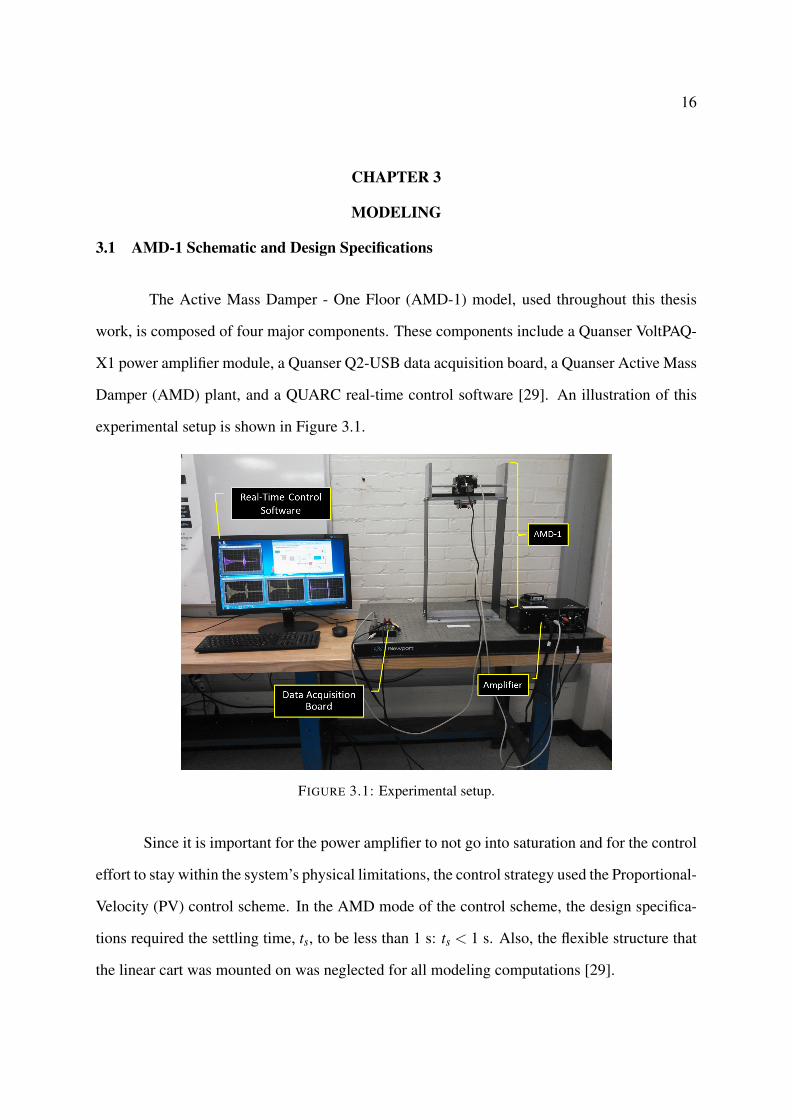
3.1 AMD-1 Schematic and Design Specifications

The Active Mass Damper - One Floor (AMD-1) model, used throughout this thesis

work, is composed of four major components. These components include a Quanser VoltPAQ-

X1 power amplifier module, a Quanser Q2-USB data acquisition board, a Quanser Active Mass

Damper (AMD) plant, and a QUARC real-time control software [29]. An illustration of this

experimental setup is shown in Figure 3.1.

FIGURE 3.1: Experimental setup.

Since it is important for the power amplifier to not go into saturation and for the control

effort to stay within the system’s physical limitations, the control strategy used the Proportional-

Velocity (PV) control scheme. In the AMD mode of the control scheme, the design specifica-

tions required the settling time, ts, to be less than 1 s: ts < 1 s. Also, the flexible structure that

the linear cart was mounted on was neglected for all modeling computations [29].

17

3.2 Equation of Motion

The equations of motion (EOM) for the (AMD-1) system are obtained from the free

body diagram. These EOM are validated by comparing them to Quanser’s EOM, which was

obtained through the Lagrange’s method. For both methods, in order to linearly model the

system, the Coulomb friction of the cart system is neglected.

When deriving the AMD-1’s dynamic model from the free body diagram method, there

were two sets of cases considered. The first set of cases considered the cart’s driving force,

Fc, produced by the motor, to be the system input. It included two cases; one ignored the

structure’s viscous damping coefficient and the other considered it as an important parameter

of the system. Since, Quanser’s derivation of the EOM also considered the system input to be

Fc and neglected the structure’s damping coefficient, the EOM obtained from this set were used

for the validating comparison.

The second set included the same cases, but the system input was considered to be the

cart motor voltage, Vm. Since all the experimental AMD-1 tests will be using the cart motor

voltage as the system input, the EOM obtained from this set were used for all the AMD-1

simulations and experimetnal tests in this thesis work.

3.2.1 Free Body Diagram

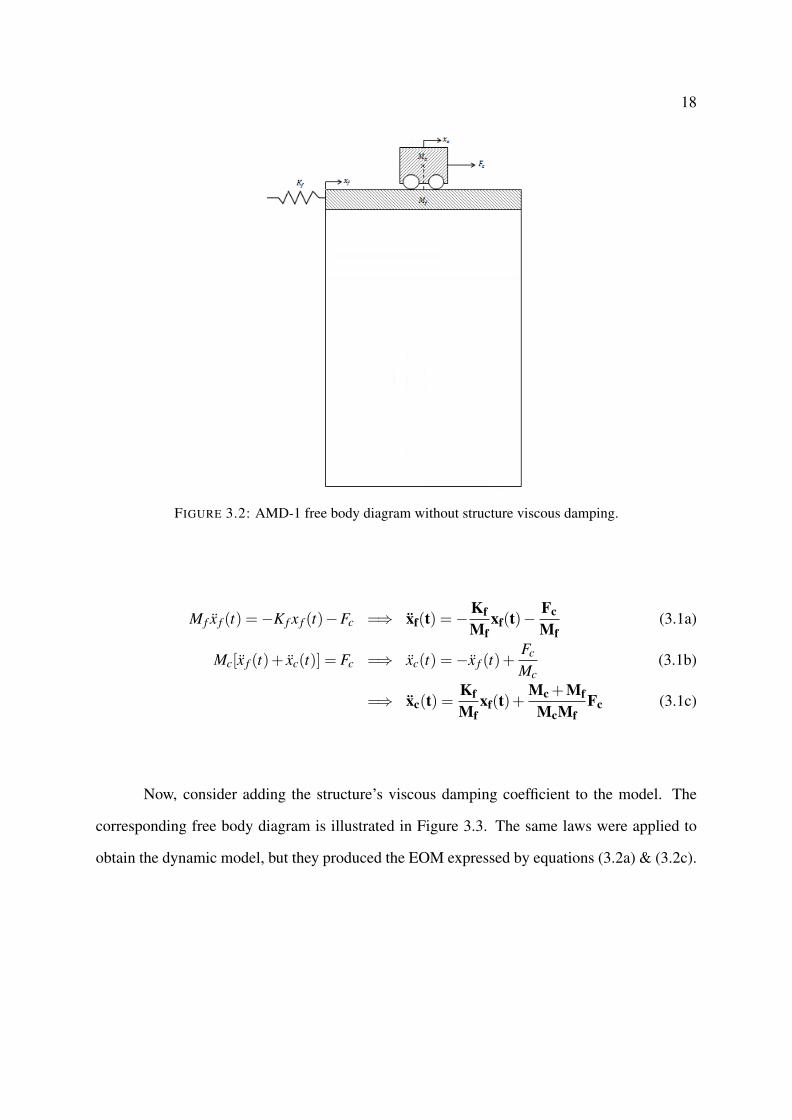
Consider the case where the structure’s viscous damping coefficient is ignored and Fc

is the system input, the corresponding AMD-1 free body diagram is illustrated in Figure 3.2.

With the application of Hooke’s law and Newton’s law of motion, the EOM in equation (3.1a)

& (3.1b) was obtained. For simplification, equation (3.1a) was substituted into equation (3.1b)

to obtain the EOM in (3.1c).

18

FIGURE 3.2: AMD-1 free body diagram without structure viscous damping.

M f x f (t) =−K f x f (t)−Fc =⇒ xf(t) =−KfMf

xf(t)−FcMf

(3.1a)

Mc[x f (t)+ xc(t)] = Fc =⇒ xc(t) =−x f (t)+Fc

Mc(3.1b)

=⇒ xc(t) =KfMf

xf(t)+Mc +Mf

McMfFc (3.1c)

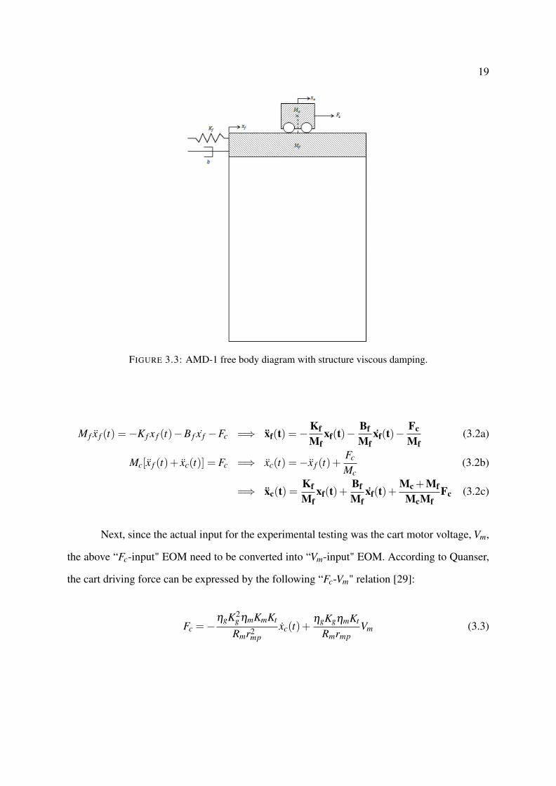
Now, consider adding the structure’s viscous damping coefficient to the model. The

corresponding free body diagram is illustrated in Figure 3.3. The same laws were applied to

obtain the dynamic model, but they produced the EOM expressed by equations (3.2a) & (3.2c).

19

FIGURE 3.3: AMD-1 free body diagram with structure viscous damping.

M f x f (t) =−K f x f (t)−B f x f −Fc =⇒ xf(t) =−KfMf

xf(t)−BfMf

xf(t)−FcMf

(3.2a)

Mc[x f (t)+ xc(t)] = Fc =⇒ xc(t) =−x f (t)+Fc

Mc(3.2b)

=⇒ xc(t) =KfMf

xf(t)+BfMf

xf(t)+Mc +Mf

McMfFc (3.2c)

Next, since the actual input for the experimental testing was the cart motor voltage, Vm,

the above “Fc-input" EOM need to be converted into “Vm-input" EOM. According to Quanser,

the cart driving force can be expressed by the following “Fc-Vm" relation [29]:

Fc =−ηgK2

g ηmKmKt

Rmr2mp

xc(t)+ηgKgηmKt

RmrmpVm (3.3)

20

After substitution and simplification, the “Vm-input" EOM for both cases were obtained. Equa-

tions (3.4a) & (3.4b) represent the EOM that ignored the structure viscous damping, and equa-

tions (3.5a) & (3.5b) represent the EOM that considered the structure viscous damping coeffi-

cient.

x f (t) =−K f

M fx f (t)+

ηgK2g ηmKmKt

Rmr2mpM f

xc(t)−ηgKgηmKt

RmrmpM fVm (3.4a)

xc(t) =K f

M fx f (t)−

ηgK2g ηmKmKt

(Mc +M f

)Rmr2

mpMcM fxc(t)+

ηgKgηmKt(Mc +M f

)RmrmpMcM f

Vm (3.4b)

x f (t) =−K f

M fx f (t)−

B f

M fx f (t)+

ηgK2g ηmKmKt

Rmr2mpM f

xc(t)−ηgKgηmKt

RmrmpM fVm (3.5a)

xc(t) =K f

M fx f (t)+

B f

M fx f (t)−

ηgK2g ηmKmKt

(Mc +M f

)Rmr2

mpMcM fxc(t)+

ηgKgηmKt(Mc +M f

)RmrmpMcM f

Vm

(3.5b)

3.2.2 Lagrange’s Method

Quanser’s Lagrangian approach was used to validate the EOM obtained from the free

body diagram. In this approach, the AMD-1 structure was modeled as a linear spring-mass

system with Fc as the single input to the system [29].

The Lagrangian, expressed as the difference between the system’s total kinetic and po-

tential energies, is expressed by equation (3.6).

L = TT −VT . (3.6)

Since the motorized linear cart’s translational direction is orthogonal to the rotor’s rotation,

the system’s total kinetic energy, TT , is expressed as the sum of the cart’s translational kinetic

21

energy, Ttc, the rotational kinetic energy of the cart motor, Trc, and the translational kinetic

energy of the flexible structure’s floor, Tt f . This summation is shown below:

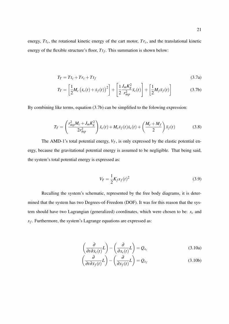
TT = Ttc +Trc +Tt f (3.7a)

TT =

[12

Mc(xc(t)+ x f (t)

)2]+

[12

JmK2g

r2mp

xc(t)

]+

[12

M f x f (t)]

(3.7b)

By combining like terms, equation (3.7b) can be simplified to the folowing expression:

TT =

(r2

mpMc + JmK2g

2r2mp

)xc(t)+Mcx f (t)xc(t)+

(Mc +M f

2

)x f (t) (3.8)

The AMD-1’s total potential energy, VT , is only expressed by the elastic potential en-

ergy, because the gravitational potential energy is assumed to be negligible. That being said,

the system’s total potential energy is expressed as:

VT =12

K f x f (t)2 (3.9)

Recalling the system’s schematic, represented by the free body diagrams, it is deter-

mined that the system has two Degrees-of-Freedom (DOF). It was for this reason that the sys-

tem should have two Lagrangian (generalized) coordinates, which were chosen to be: xc and

x f . Furthermore, the system’s Lagrange equations are expressed as:

(∂

∂ t∂ xc(t)L)−(

∂

∂xc(t)L)= Qxc (3.10a)(

∂

∂ t∂ x f (t)L)−(

∂

∂x f (t)L)= Qx f (3.10b)

22

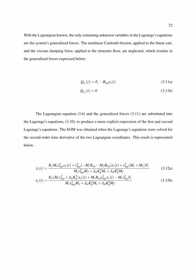
With the Lagrangian known, the only remaining unknown variables in the Lagrange’s equations

are the system’s generalized forces. The nonlinear Coulomb friction, applied to the linear cart,

and the viscous damping force, applied to the structure floor, are neglected, which resulsts in

the generalized forces expressed below:

Qxc(t) = Fc−Beqxc(t) (3.11a)

Qx f (t) = 0 (3.11b)

The Lagrangian equation (3.6) and the generalized forces (3.11) are substituted into

the Lagrange’s equations, (3.10), to produce a more explicit expression of the first and second

Lagrange’s equations. The EOM was obtained when the Lagrange’s equations were solved for

the second-order time derivative of the two Lagrangian coordinates. This result is represented

below.

xc(t) =K f Mcr2

mpx f (t)+ r2mp(−McBeq−M f Beq)xc(t)+ r2

mp(Mc +M f )Fc

Mcr2mpM f + JmK2

g Mc + JmK2g M f

(3.12a)

x f (t) =K f (Mcr2

mp + JmK2g )x f (t)+McBeqr2

mpxc(t)−Mcr2mpFc

Mcr2mpM f + JmK2

g Mc + JmK2g M f

(3.12b)

23

As a remark, when the equivalent viscous damping coefficient, Beq, as seen at the motor

pinion, and the cart rotor’s moment of inertia, Jm, are neglected, the EOM becomes:

xc(t) =K f

M fx f (t)+

Mc +M f

McM fFc (3.13a)

x f (t) =−K f

M fx f (t)−

1M f

Fc (3.13b)

Notice, when the above EOM, (3.13), is compared to the EOM in (3.1), obtained from

the first case of the free body diagram method, they are found to be identical! That being said,

validation is achieved for all EOM obtained from the free body diagram.

24

CHAPTER 4

SIMULATION

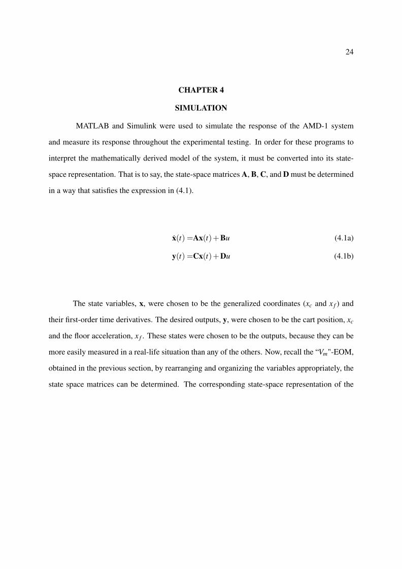
MATLAB and Simulink were used to simulate the response of the AMD-1 system

and measure its response throughout the experimental testing. In order for these programs to

interpret the mathematically derived model of the system, it must be converted into its state-

space representation. That is to say, the state-space matrices A, B, C, and D must be determined

in a way that satisfies the expression in (4.1).

x(t) =Ax(t)+Bu (4.1a)

y(t) =Cx(t)+Du (4.1b)

The state variables, x, were chosen to be the generalized coordinates (xc and x f ) and

their first-order time derivatives. The desired outputs, y, were chosen to be the cart position, xc

and the floor acceleration, x f . These states were chosen to be the outputs, because they can be

more easily measured in a real-life situation than any of the others. Now, recall the “Vm"-EOM,

obtained in the previous section, by rearranging and organizing the variables appropriately, the

state space matrices can be determined. The corresponding state-space representation of the

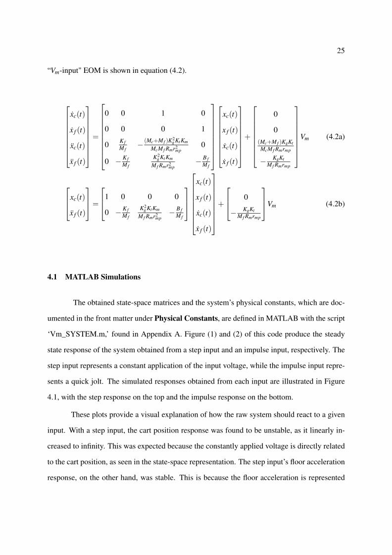
25

“Vm-input" EOM is shown in equation (4.2).

xc(t)

x f (t)

xc(t)

x f (t)

=

0 0 1 0

0 0 0 1

0 K fM f

− (Mc+M f )K2g KtKm

McM f Rmr2mp

0

0 − K fM f

K2g KtKm

M f Rmr2mp

− B fM f

xc(t)

x f (t)

xc(t)

x f (t)

+

0

0(Mc+M f )KgKtMcM f Rmrmp

− KgKtM f Rmrmp

Vm (4.2a)

xc(t)

x f (t)

=

1 0 0 0

0 − K fM f

K2g KtKm

M f Rmr2mp− B f

M f

xc(t)

x f (t)

xc(t)

x f (t)

+

0

− KgKtM f Rmrmp

Vm (4.2b)

4.1 MATLAB Simulations

The obtained state-space matrices and the system’s physical constants, which are doc-

umented in the front matter under Physical Constants, are defined in MATLAB with the script

‘Vm_SYSTEM.m,’ found in Appendix A. Figure (1) and (2) of this code produce the steady

state response of the system obtained from a step input and an impulse input, respectively. The

step input represents a constant application of the input voltage, while the impulse input repre-

sents a quick jolt. The simulated responses obtained from each input are illustrated in Figure

4.1, with the step response on the top and the impulse response on the bottom.

These plots provide a visual explanation of how the raw system should react to a given

input. With a step input, the cart position response was found to be unstable, as it linearly in-

creased to infinity. This was expected because the constantly applied voltage is directly related

to the cart position, as seen in the state-space representation. The step input’s floor acceleration

response, on the other hand, was stable. This is because the floor acceleration is represented

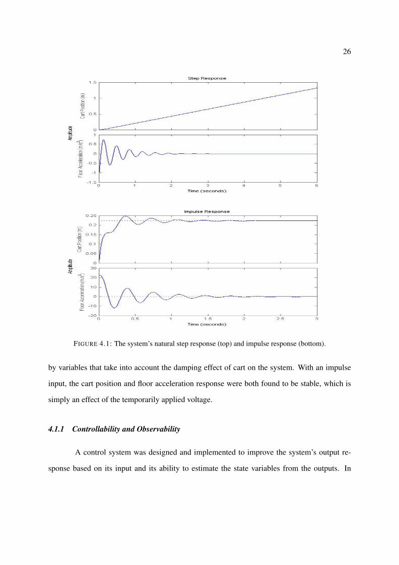
26

FIGURE 4.1: The system’s natural step response (top) and impulse response (bottom).

by variables that take into account the damping effect of cart on the system. With an impulse

input, the cart position and floor acceleration response were both found to be stable, which is

simply an effect of the temporarily applied voltage.

4.1.1 Controllability and Observability

A control system was designed and implemented to improve the system’s output re-

sponse based on its input and its ability to estimate the state variables from the outputs. In

27

order for this control system to be viable, it must be confirmed that the system is both control-

lable and observable.

A system is controllable if and only if, in a definite time interval, its states can be

modified by varying the input. This is confirmed when, the controllability matrix, CO, has full

rank. In other words, its rank must be equal to the number of system states [7, 21].

CO =

[B AB A2B A3B

](4.3)

A system is observable if and only if its states can be interpreted from its outputs. The

observability matrix, W, is used to verify this ability. Again, confirmation is achieved only

when the observability matrix has full rank [7, 21].

W =

[C CA CA2 CA3

]T

(4.4)

Both the controllability and observability matrices were computed for the AMD-1 sys-

tem, and were confirmed to have full rank, verifying that the system can be both controlled

and observed. Control was achieved through the state-feedback design and observability was

achieved through the full-order state observer design.

4.1.2 State-Feedback Design

The state-feedback design uses a full-state feedback gain vector, K, to control a system

by placing the system’s closed-loop poles at the desired pole locations. Vector K is designed

to satisfy equation (4.5), which controls the system input. After implementation of this gain

into the system, the new and improved system takes the form of equation (4.6), where the

eigenvalues of (A−BK) represent the system’s closed-loop poles.

u = Kx (4.5)

28

x = (A−BK)x (4.6)

The desired locations for these closed-loop pole are determined by the system’s de-

sired time-domain specifications. Due to the state-feedback law, these poles were placed at the

following locations:

P =

[−6+15 j −6−15 j −8 −16

]To show why these poles were chose, recal the characteristic equation of a standard second-

order system and its characteristic roots:

s2 +2ζ ωns+ω2n = 0 (4.7a)

s =−ζ ωn± jωn

√1−ζ 2 (4.7b)

The system’s damping ratio, ζ , and natural frequency, ωn, are used to determine whether

or not the system response is satisfactory, with respect to the desired time-domain specifica-

tions. With a plot of the system’s dominant pole, in the complex plane, these parameters can

be calculated. From vector P, it is established that “−6± 15 j" is the dominant pole because

e−6 has a slower decay rate than e−8 and e−16, thus having a greater influence on the system

response. The corresponding plot of this pole’s location is illustrated in Figure 4.2.

From this plot and With the use of trigonometry, the system’s parameters (ζ and ωn)

are determined from the pole’s location. Table 4.2 contains the calculated values of ζ and ωn,

along with the equations used to obtain those values.

Finally, the current system’s AMD-mode time-domain specifications can be determined

from these known parameters. Table 4.2 contains the calculated values for each specification

29

FIGURE 4.2: A plot of the system’s dominant pole and the corresponding system parameters.

TABLE 4.1: System Parameters Obtained from the Pole Plot

Specification Equation ValueNatural Frequency Re2 + Im2 = ω2

n ωn = 16.1555 HzDamping Ratio Re = ωnζ ζ = .37139

along with the formulas used to obtain them. Recall the AMD-mode settling time design spec-

ification: ts ≤ 1s, stated in the previous section titled Experimental Setup and Specifications.

From the table’s settling time value, it is concluded that the system’s peak time performance

was satisfactory because it settled in about .6667 s, which is faster than specified.

TABLE 4.2: Time-Domain Specifications Obtained from the System Parameters

Specification Equation ValueSettling Time ts = 4

ζ ωnts = .667 s

Peak Time tp =π

ωn√

1−ζ 2tp = .209 s

Percent Overshoot Mp = e

(−πζ√1−ζ 2

)Mp = 28.461 %

30

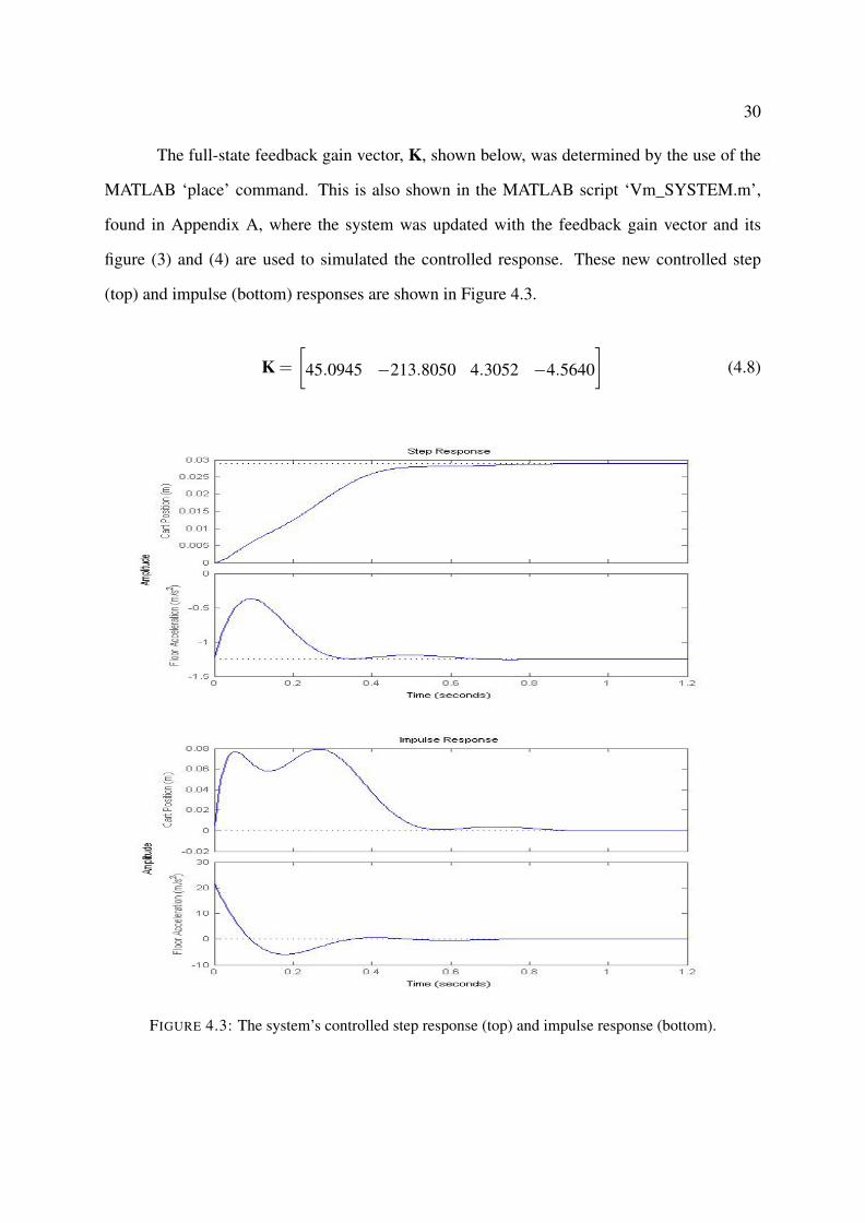
The full-state feedback gain vector, K, shown below, was determined by the use of the

MATLAB ‘place’ command. This is also shown in the MATLAB script ‘Vm_SYSTEM.m’,

found in Appendix A, where the system was updated with the feedback gain vector and its

figure (3) and (4) are used to simulated the controlled response. These new controlled step

(top) and impulse (bottom) responses are shown in Figure 4.3.

K =

[45.0945 −213.8050 4.3052 −4.5640

](4.8)

FIGURE 4.3: The system’s controlled step response (top) and impulse response (bottom).

31

A comparison of these controlled responses with the natural responses, of Figure 4.1,

indicates that the use of vector K was successful. First consider the responses obtained from

the step input (a constant voltage). The natural cart position response was unstable, but when

the feedback gain is applied to the system, its response is stabilized, leveling off at about .o3 m.

The floor acceleration response, although already stable in its natural state, showed an improved

decay rate with the application of the feedback gain. The natural floor acceleration response

took about 3 s to decay, but after the feedback gain was added, it decayed in less than 1 s.

Now consider the responses obtained from the impulse input (a voltage jolt). The natural

response of the cart position peaked at .25 m and only decayed to about .225 m. With the

feedback gain, the peak only reached .08 m and it decayed all the way to 0 m. Just as in the

step responses, the effect of the feedback gain, on the floor acceleration was an improved decay

rate. It decreased its decay time from 3 s to about .8 s.

4.1.3 Full-Order State Observer Design

According to the full-state feedback law, since only the floor acceleration is directly

measured, the AMD-1’s active control strategy should also incorporate a state observer. This

design specification was chosen to more accurately represent a full-scale application, where the

floor deflection or velocity are very difficult to measure. Accelerometers, provide affordable

and reliable means of sensing a structure’s dynamic behavior, and they produce measurements

that can be used to estimate the floor deflection and velocity.

The observer is designed to satisfy equation (4.9), and is essentially a replica of the

actual plant, but with a corrective term that gets multiplied by the full-order observer gain

32

matrix, G.

X0 =AX0 +BU+G(Y−Y0) (4.9a)

Y0 =CX0 +DU (4.9b)

Vector G was determined by placing the closed-loop poles at the locations specified by

vector OP. These locations were chosen based on the observer error dynamics. It ensures that

there will be no interference from the observer on the plant’s dynamics, and was chosen to

make the observer error dynamics over three times faster than the plant’s error dynamics.

OP =

[−20 −25 −30 −35

]The MATLAB script ‘Vm_SYSTEM.m’, found in Appendix A, was also used to de-

termine the value of the full-order observer gain matrix, G, and to update the system with the

observer gain. Visual plots illustrating the actual and estimated states will be provided in the

Simulink section.

G =

36.6829 0.0036

−4.7604 −0.1765

107.6736 −0.7844

−243.1164 −1.5950

(4.10)

33

4.2 Simulink Simulations

To accompany and support the above MATLAB responses, corresponding Simulink

diagrams were constructed for the system’s response to a step-input. The open-loop, closed-

loop, and state observer diagrams are presented and used to simulate and analyze the system’s

output responses.

4.2.1 Open-Loop

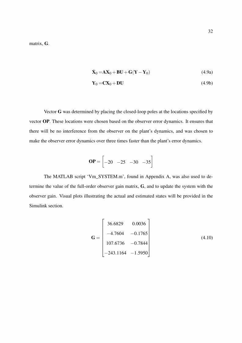
Figure 4.4 represents the open-loop model of the AMD-1 system. The state-space

matrices (A, B, C, and D) were uploaded, with the previously mentioned MATLAB scripts,

and the scope was used to plot its response.

FIGURE 4.4: Open-loop Simulink diagram.

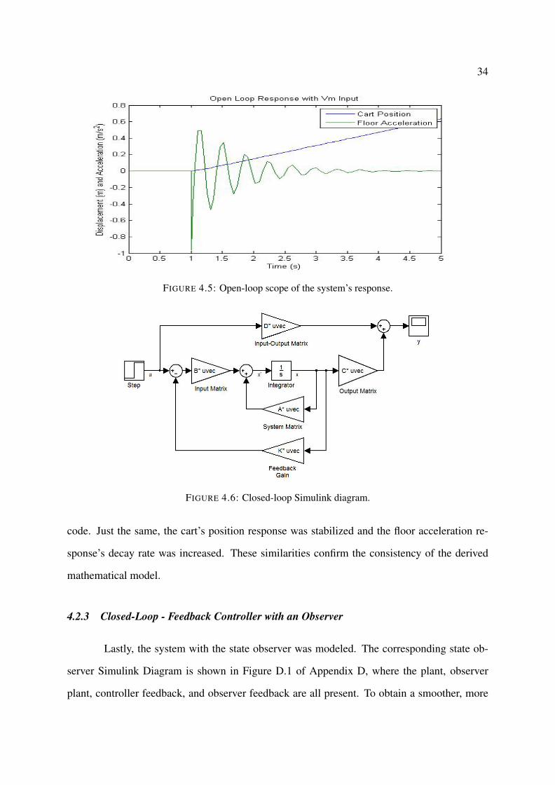
Figure 4.5 illustrates the response of the open-loop system. Notice, both the cart posi-

tion and floor acceleration responses perfectly match those obtained from the MATLAB code,

but they are plotted on the same graph. Just the same, the cart’s position response is unstable,

increasing toward infinity, and the floor acceleration response is stable, decaying over time.

4.2.2 Closed-Loop - Feedback Controller

Just as before, the system needs to be controlled. Control is achieved by adding the

feedback gain, K, to the system. Doing so, resulted in the closed-loop Simulink diagram,

illustrated in Figure 4.6. Again, the corresponding state space matrices and feedback gain

vector were uploaded, and the scope was used to plot the system’s response.

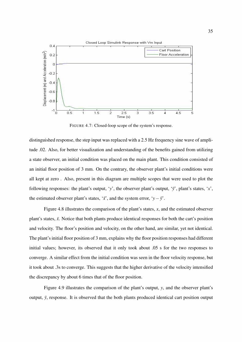
Figure 4.7 illustrates the controlled response obtained from the closed-loop system.

Again, both output responses were proved to be identical to those obtained from the MATLAB

34

FIGURE 4.5: Open-loop scope of the system’s response.

FIGURE 4.6: Closed-loop Simulink diagram.

code. Just the same, the cart’s position response was stabilized and the floor acceleration re-

sponse’s decay rate was increased. These similarities confirm the consistency of the derived

mathematical model.

4.2.3 Closed-Loop - Feedback Controller with an Observer

Lastly, the system with the state observer was modeled. The corresponding state ob-

server Simulink Diagram is shown in Figure D.1 of Appendix D, where the plant, observer

plant, controller feedback, and observer feedback are all present. To obtain a smoother, more

35

FIGURE 4.7: Closed-loop scope of the system’s response.

distinguished response, the step input was replaced with a 2.5 Hz frequency sine wave of ampli-

tude .02. Also, for better visualization and understanding of the benefits gained from utilizing

a state observer, an initial condition was placed on the main plant. This condition consisted of

an initial floor position of 3 mm. On the contrary, the observer plant’s initial conditions were

all kept at zero . Also, present in this diagram are multiple scopes that were used to plot the

following responses: the plant’s output, ‘y’, the observer plant’s output, ‘y’, plant’s states, ‘x’,

the estimated observer plant’s states, ‘x’, and the system error, ‘y− y’.

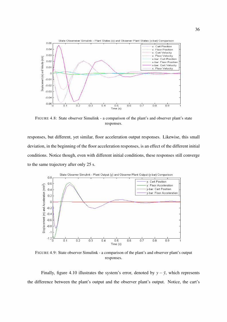
Figure 4.8 illustrates the comparison of the plant’s states, x, and the estimated observer

plant’s states, x. Notice that both plants produce identical responses for both the cart’s position

and velocity. The floor’s position and velocity, on the other hand, are similar, yet not identical.

The plant’s initial floor position of 3 mm, explains why the floor position responses had different

initial values; however, its observed that it only took about .05 s for the two responses to

converge. A similar effect from the initial condition was seen in the floor velocity response, but

it took about .3s to converge. This suggests that the higher derivative of the velocity intensified

the discrepancy by about 6 times that of the floor position.

Figure 4.9 illustrates the comparison of the plant’s output, y, and the observer plant’s

output, y, response. It is observed that the both plants produced identical cart position output

36

FIGURE 4.8: State observer Simulink - a comparison of the plant’s and observer plant’s stateresponses.

responses, but different, yet similar, floor acceleration output responses. Likewise, this small

deviation, in the beginning of the floor acceleration responses, is an effect of the different initial

conditions. Notice though, even with different initial conditions, these responses still converge

to the same trajectory after only 25 s.

FIGURE 4.9: State observer Simulink - a comparison of the plant’s and observer plant’s outputresponses.

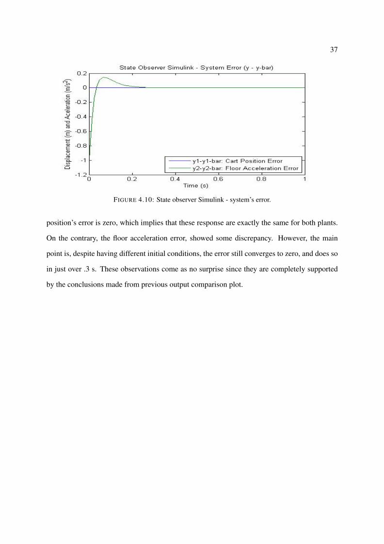
Finally, figure 4.10 illustrates the system’s error, denoted by y− y, which represents

the difference between the plant’s output and the observer plant’s output. Notice, the cart’s

37

FIGURE 4.10: State observer Simulink - system’s error.

position’s error is zero, which implies that these response are exactly the same for both plants.

On the contrary, the floor acceleration error, showed some discrepancy. However, the main

point is, despite having different initial conditions, the error still converges to zero, and does so

in just over .3 s. These observations come as no surprise since they are completely supported

by the conclusions made from previous output comparison plot.

38

CHAPTER 5

PARAMETER ESTIMATION

Since the viscous damping coefficient of the structure, B f , was neglected in all the

previous simulations, parameter estimation techniques were used to obtain a more accurate

model of the system. The two techniques considered for this estimation included a Simulink

Parameter Estimation Toolbox and an external motion and force sensor.

5.1 Simulink Toolbox

Figure 5.1 illustrates the Simulink diagram that incorporated the Simulink Parameter

Estimation Toolbox. It included a basic model of the AMD-1’s mass-spring-damper system,

a ‘Parameter Estimation GUI with preloaded data’ toolbox, a transient data block, and a sys-

tem parameter block, which contains their current values. Within the transient data block was

preloaded floor position data that was obtained from an experimental test on the AMD-1 struc-

ture. The scope, shown in Figure 5.2, illustrates the plots of the unstable simulated floor position

response and the preloaded experimental floor position data, both of which had an initial floor

position of 12.0126 mm.

The presented GUI toolbox contained a ‘Control and Estimation Tools Manager,’ which

is where the parameter estimation project was created. It performed a number of continuous

parameter estimation iterations until the simulated response converged to take a form similar

to response produced by the transient data. In this case, the estimation tool performed 100

iterations, where the final values of the estimated parameters were: M f = 2.509 kg, B f = 3.283

Ns/m, and K f = 511.9 N/m. The resultant plot of the estimator is plotted with the transient data

in Figure 5.3, where it is observed that the two responses very closely resemble each other.

39

FIGURE 5.1: Simulink model of the AMD-1’s mass-spring-damper system with parameterestimation GUI.

FIGURE 5.2: A comparison of the simulated and experimental floor position data before esti-mation.

5.1.1 External Sensor Tests

An external motion and force sensor was also used to estimate the system parameters.

The setup of these sensors, with respect to the AMD-1 model, is illustrated in Figure 5.4. Here,

the motion sensor was supported by a tripod, which was positioned at the height of the AMD-

1’s top floor, and the force sensor, was tied to the top of the structure’s wall with fishing line. In

40

FIGURE 5.3: A comparison of the experimental and estimated floor position response afterestimation.

addition, both sensors were connected to the computer, where real-time data was unanimously

collected.

FIGURE 5.4: Force and motion sensor setup.

With both sensors turned on, an impulse excitation was applied to the AMD-1 structure

by quickly pulling the force sensor away from the model and immediately letting go. A plot of

the collected sensor data is illustrated in Figure 5.5, where the data tips represent the important

values that were used to calculate the system parameters. From this data K f was derived from

41

Hooke’s law, M f was derived from the natural frequency formula, and B f was derived from the

logarithmic decrement.

FIGURE 5.5: Force and motion sensor response as an impulse force was applied to the AMD-1structure.

Table 5.1 organizes and defines the variables obtained from the sensor data and the

calculations used to derive K f and M f . From the force sensor’s plot, the maximum applied

force, Fmax, was easily found by the value at the tip of the single peak. Note, the reason that this

peak is negative is simply because the force sensor was pulled to the left. The time at which

this maximum force was applied was used to obtain the corresponding floor position, x f orce.

However, this position is not the actual displacement of the floor. Notice, at rest, the sensor

data shows that the floor position is at .42 m, which is the distance between the sensor and the

floor. Therefore, that distance must be subtracted from x f orce to get the actual displacement of

the floor. This value, along with Fmax was used in Hook’s law to calculate K f .

Next, the period, T , of the position sensor’s response was measured and used to calcu-

late the natural frequency of the system, ωn. This value, along with the previously calculated

stiffness, were used to obtain M f with the natural frequency formula expressed in Table 5.1.

Table 5.2 formulates the derivation of B f . Presented is the calculation of the system’s

free response. From this response, the logarithmic decrement, δ , was found, which is defined

42

TABLE 5.1: Derivation of the Floor’s Stiffness and Mass

Variable Symbol Value CalculationsMaximum Force Applied Fmax -17.8629 N F = kxDistance Between Sensor and AMD-1 xs .42 m K f =

Fmaxx f orce−xs

Floor Position at Time of Fmax x f orce .382 m Kf = 470.0763 N/m

Period T .375 s ωn =√

K fM f

Frequency f =1/T 8/3 Hz M2f =

K f

M2f

Natural Frequency ωn = 2π f 16π

3 rad/s Mf = 1.6744 kg

as the natural logarithm of the ratio of two consecutive amplitudes. The value of δ was obtained

through the graphical approach, which uses the measurements of peak one and six (shown by

the data tips in Figure 5.5). With this value, the damping ratio was calculated through the

numerical approach. Then finally, with the damping ration, the floors mass, and the floors

stiffness, B f was determined.

TABLE 5.2: Derivation of the Floor’s Damping Coefficient, Graph: [18]

Calculation of the System’s Free Response:mx+2ζ ωnx+ω2

n x = 0

xT (t) = X0e−ζ ωnt sin(2π f t +φ)

Logarithmic Decrement: δ = ln x(t)x(t+T )

↙ ↘Graphical Approach Numerical Approach

δ = 1n ln x1

xn+1δ = ln 2πζ√

1−ζ 2

δ = 15 ln .469−.42

.437−.42 ζ = δ√4π2+δ 2

δ = .2117−→ ζ = .2117√4π2+.21172

ζ = .03368

B f = 2ζ√

M f K f

Bf = 1.8898 Ns/m

43

CHAPTER 6

RESULTS

6.1 Experimental Testing

All the experimental tests were performed on a single story building model. Recall

Figure 3.1, where it shows the AMD-1 model connected to a computer installed with the real-

time control software, QUARC. This software was used in the Simulink Model, shown in Figure

D.2 of Appendix D, to run the experimental tests and collect the response data, which included

the floor’s position and acceleration, the cart motor voltage, and the cart position.

To obtain these responses, the necessary system parameter and state-space matrix values

were defined within the Simulink model with a provided set of MATLAB scripts [29]. As

improvements were made to the system, these scripts were updated and modified with the

MATLAB scripts documented in the Appendix.

Notice, the mode switching sequence incorporated in this model. It is used to alternate

between the structure excitation mode and the active mass damping mode. Initially, this se-

quence was programmed to excite the AMD-1 structure at 0 s, and again at 11.5 s, and then

also dampen it at 11.5 s. In other words, the controller was off during the first excitation, and

then turned on, at 11.5 s, for the second excitation. The purpose of this was to provide a clear

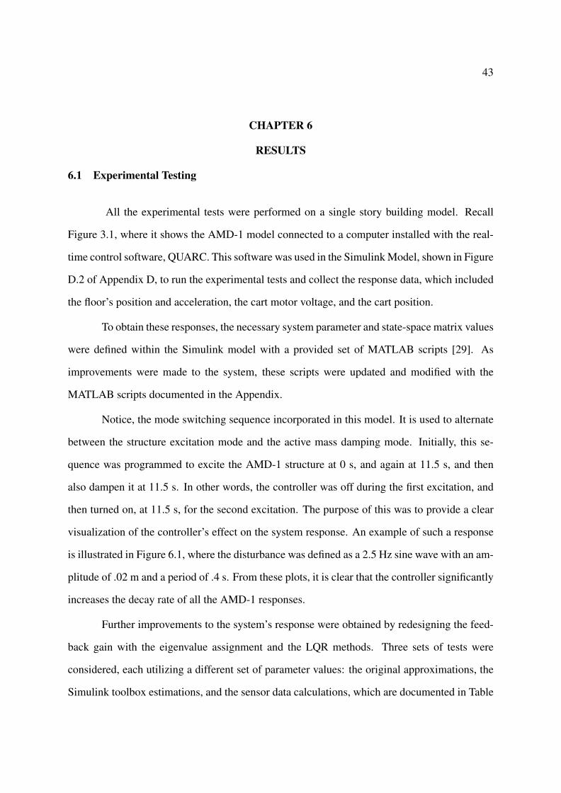
visualization of the controller’s effect on the system response. An example of such a response

is illustrated in Figure 6.1, where the disturbance was defined as a 2.5 Hz sine wave with an am-

plitude of .02 m and a period of .4 s. From these plots, it is clear that the controller significantly

increases the decay rate of all the AMD-1 responses.

Further improvements to the system’s response were obtained by redesigning the feed-

back gain with the eigenvalue assignment and the LQR methods. Three sets of tests were

considered, each utilizing a different set of parameter values: the original approximations, the

Simulink toolbox estimations, and the sensor data calculations, which are documented in Table

44

FIGURE 6.1: Floor position and acceleration, cart position, and cart motor voltage responses.

6.1. The corresponding gains for each set were determined and applied to the system, where

simulated and experimental tests were analyzed.

TABLE 6.1: The Sets of System Parameters Values Used for Testing

System Parameters Floor Mass M f Structure Damping B f Floor Stiffness K f

(kg) (Ns/m) (N/m)Original Approximations: 1.3800 0.0000 500.9000Simulink Estimations: 2.5090 3.2830 511.6000Sensor Calculations: 1.6744 1.8898 470.0763

6.2 Estimated vs. Original Parameter Tests

To test the validity of the Simulink parameter estimations, their responses were com-

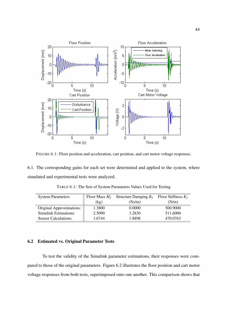
pared to those of the original parameters. Figure 6.2 illustrates the floor position and cart motor

voltage responses from both tests, superimposed onto one another. This comparison shows that

45

both sets of parameters seem to produce similar responses, but the estimated parameter test

does appear have a slightly wider range of fluctuation.

FIGURE 6.2: A comparison of the floor position (left) and cart motor voltage (right) dataobtained from the original vs. estimated parameters.

To further analyze this comparison, the RMS values were calculated for each response.

These values are displayed in Table 6.2, where it is observed that, for both the floor position and

cart motor voltage results, the RMS values were smaller for the results obtained from the orig-

inal parameter test. Furthermore, since the estimated parameter tests showed no improvement

in the system response, further use of them was concluded to be unnecessary.

TABLE 6.2: RMS Values of the Original and Estimated Parameter Test Responses

Parameters Floor Position RMS Cart Motor Voltage RMSOriginal 3.2197 0.4987Estimated 3.5818 0.5017

6.3 Eigenvalue Assignment Results

The first method used to redesign the feedback control was the eigenvalue assignment

method. This method improves the system response by focusing on increasing the response’s

46

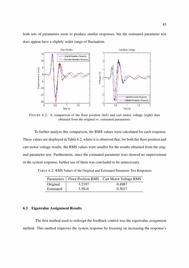
peak ratio reduction. As previously stated, the control theory says that this is done by mov-

ing the location of the system’s dominant poles further to the left in the complex plane, where

the dominant poles are the ones that produce the exponential function with the slowest de-

cay rate. Recall, the AMD-1 system’s pole locations, represented by: P = [−6+ 15 j,−6−

15 j,−8,−16]. Figure 6.3 illustrates the exponential functions produced by the real poles, -8

and -16, and the real part of the complex poles, -6. From this plot, it is evident that the dominant

poles are “−6±15".

FIGURE 6.3: A plot of the exponential function provided by the closed-loop poles.

Due to certain constraints, the range for which these roots can be varied is limited. The

lower variation limit is determined by the stability boundary, which is defined by the imaginary

(or vertical) axis of the complex plane. The upper variation limit is determined by Earthly

limitations, such as the availability of voltage, money, and resources. Figure 6.4 illustrates the

location of each set of poles considered for the eigenvalue assignment tests.

Investigation into the effect the pole location has on the feedback design, and the effect

the gain has on the AMD-1 system response, was analyzed through two sets of simulated and

experimental tests. One test modeled the system with the original parameters and the other used

the parameters calculated from the sensor tests. To update the plant and control system with

the appropriate parameters and modifications, the MATLAB script ‘EIGENVALUE.m,’ found

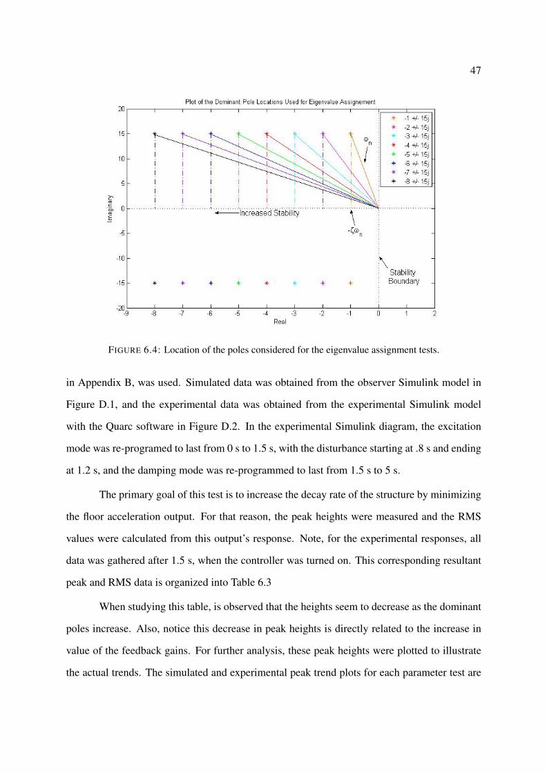
47

FIGURE 6.4: Location of the poles considered for the eigenvalue assignment tests.

in Appendix B, was used. Simulated data was obtained from the observer Simulink model in

Figure D.1, and the experimental data was obtained from the experimental Simulink model

with the Quarc software in Figure D.2. In the experimental Simulink diagram, the excitation

mode was re-programed to last from 0 s to 1.5 s, with the disturbance starting at .8 s and ending

at 1.2 s, and the damping mode was re-programmed to last from 1.5 s to 5 s.

The primary goal of this test is to increase the decay rate of the structure by minimizing

the floor acceleration output. For that reason, the peak heights were measured and the RMS

values were calculated from this output’s response. Note, for the experimental responses, all

data was gathered after 1.5 s, when the controller was turned on. This corresponding resultant

peak and RMS data is organized into Table 6.3

When studying this table, is observed that the heights seem to decrease as the dominant

poles increase. Also, notice this decrease in peak heights is directly related to the increase in

value of the feedback gains. For further analysis, these peak heights were plotted to illustrate

the actual trends. The simulated and experimental peak trend plots for each parameter test are

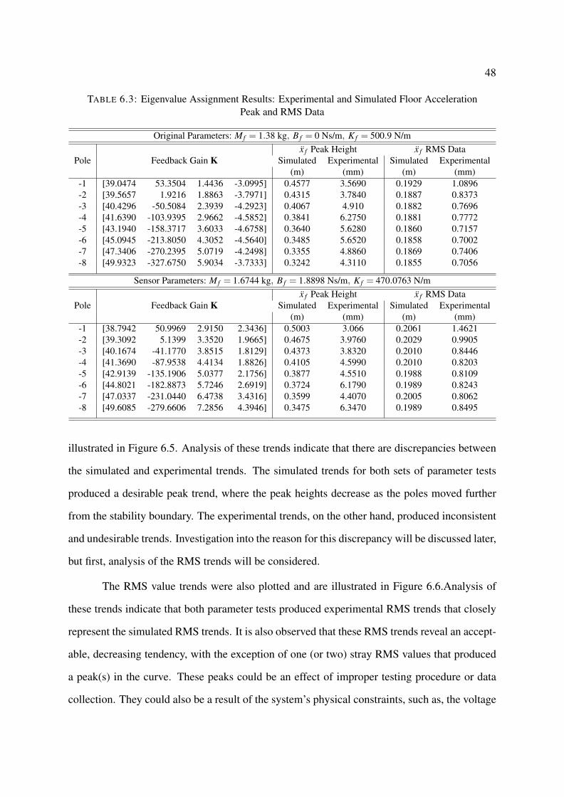
48

TABLE 6.3: Eigenvalue Assignment Results: Experimental and Simulated Floor AccelerationPeak and RMS Data

Original Parameters: M f = 1.38 kg, B f = 0 Ns/m, K f = 500.9 N/mx f Peak Height x f RMS Data

Pole Feedback Gain K Simulated Experimental Simulated Experimental(m) (mm) (m) (mm)

-1 [39.0474 53.3504 1.4436 -3.0995] 0.4577 3.5690 0.1929 1.0896-2 [39.5657 1.9216 1.8863 -3.7971] 0.4315 3.7840 0.1887 0.8373-3 [40.4296 -50.5084 2.3939 -4.2923] 0.4067 4.910 0.1882 0.7696-4 [41.6390 -103.9395 2.9662 -4.5852] 0.3841 6.2750 0.1881 0.7772-5 [43.1940 -158.3717 3.6033 -4.6758] 0.3640 5.6280 0.1860 0.7157-6 [45.0945 -213.8050 4.3052 -4.5640] 0.3485 5.6520 0.1858 0.7002-7 [47.3406 -270.2395 5.0719 -4.2498] 0.3355 4.8860 0.1869 0.7406-8 [49.9323 -327.6750 5.9034 -3.7333] 0.3242 4.3110 0.1855 0.7056

Sensor Parameters: M f = 1.6744 kg, B f = 1.8898 Ns/m, K f = 470.0763 N/mx f Peak Height x f RMS Data

Pole Feedback Gain K Simulated Experimental Simulated Experimental(m) (mm) (m) (mm)

-1 [38.7942 50.9969 2.9150 2.3436] 0.5003 3.066 0.2061 1.4621-2 [39.3092 5.1399 3.3520 1.9665] 0.4675 3.9760 0.2029 0.9905-3 [40.1674 -41.1770 3.8515 1.8129] 0.4373 3.8320 0.2010 0.8446-4 [41.3690 -87.9538 4.4134 1.8826] 0.4105 4.5990 0.2010 0.8203-5 [42.9139 -135.1906 5.0377 2.1756] 0.3877 4.5510 0.1988 0.8109-6 [44.8021 -182.8873 5.7246 2.6919] 0.3724 6.1790 0.1989 0.8243-7 [47.0337 -231.0440 6.4738 3.4316] 0.3599 4.4070 0.2005 0.8062-8 [49.6085 -279.6606 7.2856 4.3946] 0.3475 6.3470 0.1989 0.8495

illustrated in Figure 6.5. Analysis of these trends indicate that there are discrepancies between

the simulated and experimental trends. The simulated trends for both sets of parameter tests

produced a desirable peak trend, where the peak heights decrease as the poles moved further

from the stability boundary. The experimental trends, on the other hand, produced inconsistent

and undesirable trends. Investigation into the reason for this discrepancy will be discussed later,

but first, analysis of the RMS trends will be considered.

The RMS value trends were also plotted and are illustrated in Figure 6.6.Analysis of

these trends indicate that both parameter tests produced experimental RMS trends that closely

represent the simulated RMS trends. It is also observed that these RMS trends reveal an accept-

able, decreasing tendency, with the exception of one (or two) stray RMS values that produced

a peak(s) in the curve. These peaks could be an effect of improper testing procedure or data

collection. They could also be a result of the system’s physical constraints, such as, the voltage

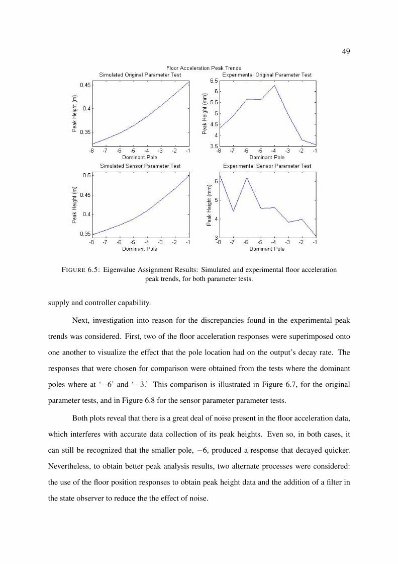
49

FIGURE 6.5: Eigenvalue Assignment Results: Simulated and experimental floor accelerationpeak trends, for both parameter tests.

supply and controller capability.

Next, investigation into reason for the discrepancies found in the experimental peak

trends was considered. First, two of the floor acceleration responses were superimposed onto

one another to visualize the effect that the pole location had on the output’s decay rate. The

responses that were chosen for comparison were obtained from the tests where the dominant

poles where at ‘−6’ and ‘−3.’ This comparison is illustrated in Figure 6.7, for the original

parameter tests, and in Figure 6.8 for the sensor parameter parameter tests.

Both plots reveal that there is a great deal of noise present in the floor acceleration data,

which interferes with accurate data collection of its peak heights. Even so, in both cases, it

can still be recognized that the smaller pole, −6, produced a response that decayed quicker.

Nevertheless, to obtain better peak analysis results, two alternate processes were considered:

the use of the floor position responses to obtain peak height data and the addition of a filter in

the state observer to reduce the the effect of noise.

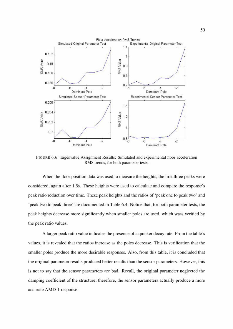
50

FIGURE 6.6: Eigenvalue Assignment Results: Simulated and experimental floor accelerationRMS trends, for both parameter tests.

When the floor position data was used to measure the heights, the first three peaks were

considered, again after 1.5s. These heights were used to calculate and compare the response’s

peak ratio reduction over time. These peak heights and the ratios of ‘peak one to peak two’ and

‘peak two to peak three’ are documented in Table 6.4. Notice that, for both parameter tests, the

peak heights decrease more significantly when smaller poles are used, which wass verified by

the peak ratio values.

A larger peak ratio value indicates the presence of a quicker decay rate. From the table’s

values, it is revealed that the ratios increase as the poles decrease. This is verification that the

smaller poles produce the more desirable responses. Also, from this table, it is concluded that

the original parameter results produced better results than the sensor parameters. However, this

is not to say that the sensor parameters are bad. Recall, the original parameter neglected the

damping coefficient of the structure; therefore, the sensor parameters actually produce a more

accurate AMD-1 response.

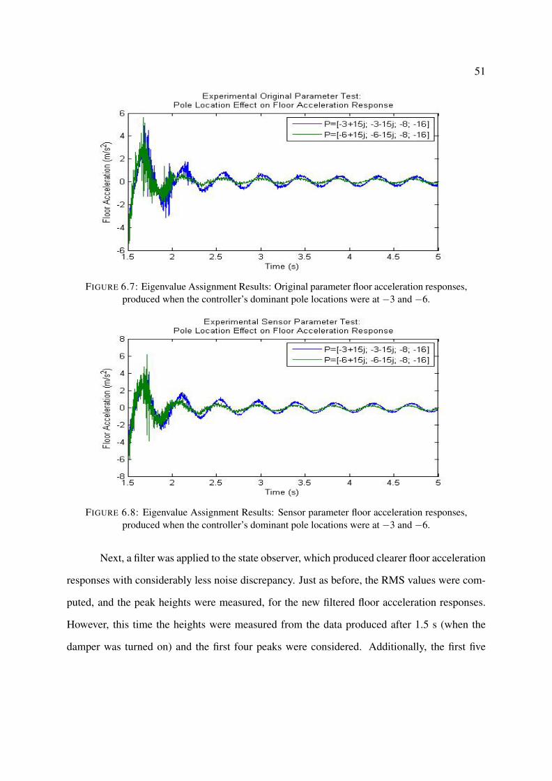
51

FIGURE 6.7: Eigenvalue Assignment Results: Original parameter floor acceleration responses,produced when the controller’s dominant pole locations were at −3 and −6.

FIGURE 6.8: Eigenvalue Assignment Results: Sensor parameter floor acceleration responses,produced when the controller’s dominant pole locations were at −3 and −6.

Next, a filter was applied to the state observer, which produced clearer floor acceleration

responses with considerably less noise discrepancy. Just as before, the RMS values were com-

puted, and the peak heights were measured, for the new filtered floor acceleration responses.

However, this time the heights were measured from the data produced after 1.5 s (when the

damper was turned on) and the first four peaks were considered. Additionally, the first five

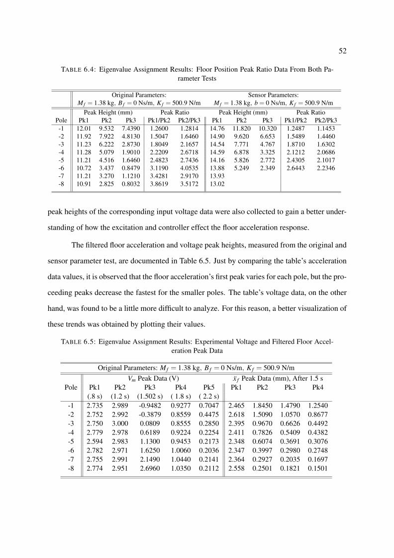
52

TABLE 6.4: Eigenvalue Assignment Results: Floor Position Peak Ratio Data From Both Pa-rameter Tests

Original Parameters: Sensor Parameters:M f = 1.38 kg, B f = 0 Ns/m, K f = 500.9 N/m M f = 1.38 kg, b = 0 Ns/m, K f = 500.9 N/m

Peak Height (mm) Peak Ratio Peak Height (mm) Peak RatioPole Pk1 Pk2 Pk3 Pk1/Pk2 Pk2/Pk3 Pk1 Pk2 Pk3 Pk1/Pk2 Pk2/Pk3-1 12.01 9.532 7.4390 1.2600 1.2814 14.76 11.820 10.320 1.2487 1.1453-2 11.92 7.922 4.8130 1.5047 1.6460 14.90 9.620 6.653 1.5489 1.4460-3 11.23 6.222 2.8730 1.8049 2.1657 14.54 7.771 4.767 1.8710 1.6302-4 11.28 5.079 1.9010 2.2209 2.6718 14.59 6.878 3.325 2.1212 2.0686-5 11.21 4.516 1.6460 2.4823 2.7436 14.16 5.826 2.772 2.4305 2.1017-6 10.72 3.437 0.8479 3.1190 4.0535 13.88 5.249 2.349 2.6443 2.2346-7 11.21 3.270 1.1210 3.4281 2.9170 13.93-8 10.91 2.825 0.8032 3.8619 3.5172 13.02

peak heights of the corresponding input voltage data were also collected to gain a better under-

standing of how the excitation and controller effect the floor acceleration response.

The filtered floor acceleration and voltage peak heights, measured from the original and

sensor parameter test, are documented in Table 6.5. Just by comparing the table’s acceleration

data values, it is observed that the floor acceleration’s first peak varies for each pole, but the pro-

ceeding peaks decrease the fastest for the smaller poles. The table’s voltage data, on the other

hand, was found to be a little more difficult to analyze. For this reason, a better visualization of

these trends was obtained by plotting their values.

TABLE 6.5: Eigenvalue Assignment Results: Experimental Voltage and Filtered Floor Accel-eration Peak Data

Original Parameters: M f = 1.38 kg, B f = 0 Ns/m, K f = 500.9 N/mVm Peak Data (V) x f Peak Data (mm), After 1.5 s

Pole Pk1 Pk2 Pk3 Pk4 Pk5 Pk1 Pk2 Pk3 Pk4(.8 s) (1.2 s) (1.502 s) ( 1.8 s) ( 2.2 s)

-1 2.735 2.989 -0.9482 0.9277 0.7047 2.465 1.8450 1.4790 1.2540-2 2.752 2.992 -0.3879 0.8559 0.4475 2.618 1.5090 1.0570 0.8677-3 2.750 3.000 0.0809 0.8555 0.2850 2.395 0.9670 0.6626 0.4492-4 2.779 2.978 0.6189 0.9224 0.2254 2.411 0.7826 0.5409 0.4382-5 2.594 2.983 1.1300 0.9453 0.2173 2.348 0.6074 0.3691 0.3076-6 2.782 2.971 1.6250 1.0060 0.2036 2.347 0.3997 0.2980 0.2748-7 2.755 2.991 2.1490 1.0440 0.2141 2.364 0.2927 0.2035 0.1697-8 2.774 2.951 2.6960 1.0350 0.2112 2.558 0.2501 0.1821 0.1501

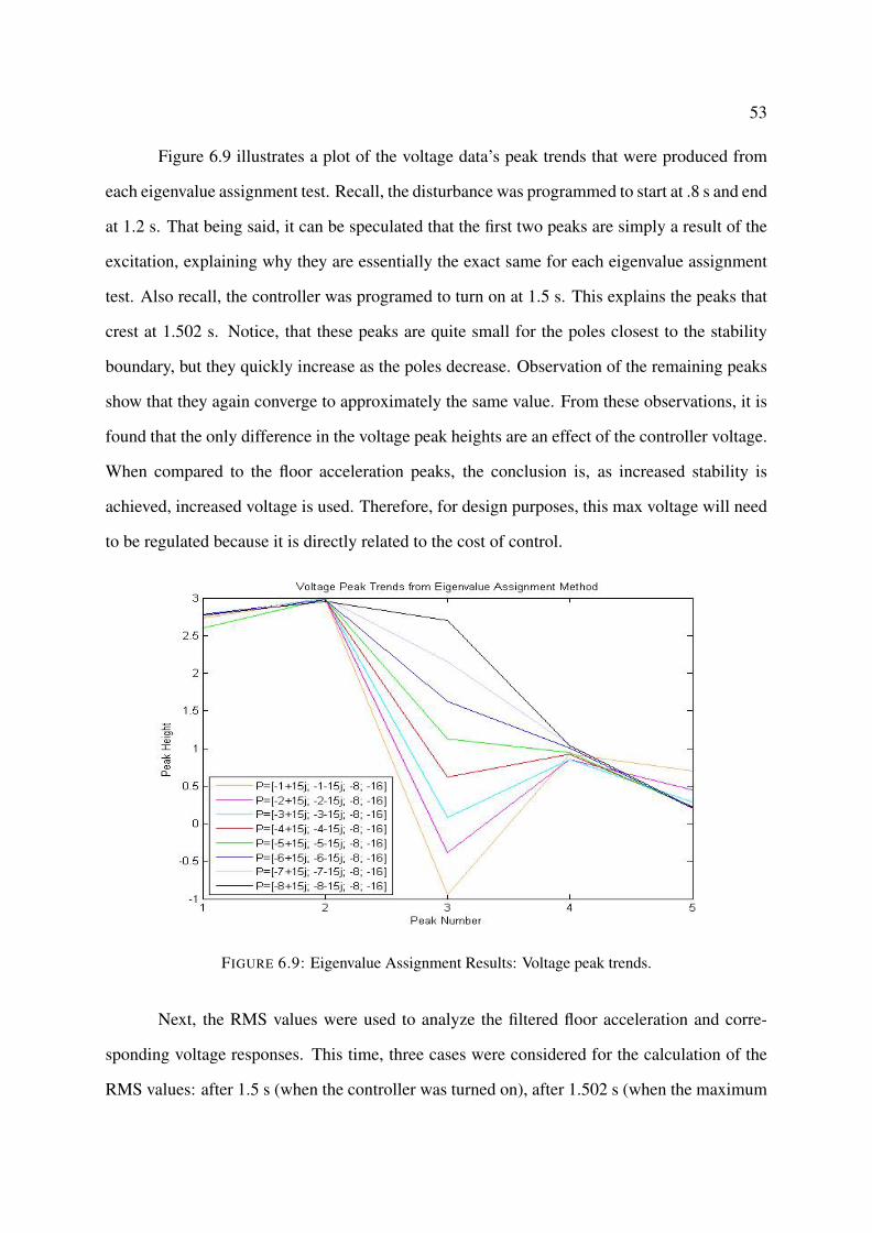
53

Figure 6.9 illustrates a plot of the voltage data’s peak trends that were produced from

each eigenvalue assignment test. Recall, the disturbance was programmed to start at .8 s and end

at 1.2 s. That being said, it can be speculated that the first two peaks are simply a result of the

excitation, explaining why they are essentially the exact same for each eigenvalue assignment

test. Also recall, the controller was programed to turn on at 1.5 s. This explains the peaks that

crest at 1.502 s. Notice, that these peaks are quite small for the poles closest to the stability

boundary, but they quickly increase as the poles decrease. Observation of the remaining peaks

show that they again converge to approximately the same value. From these observations, it is

found that the only difference in the voltage peak heights are an effect of the controller voltage.

When compared to the floor acceleration peaks, the conclusion is, as increased stability is

achieved, increased voltage is used. Therefore, for design purposes, this max voltage will need

to be regulated because it is directly related to the cost of control.

FIGURE 6.9: Eigenvalue Assignment Results: Voltage peak trends.

Next, the RMS values were used to analyze the filtered floor acceleration and corre-

sponding voltage responses. This time, three cases were considered for the calculation of the

RMS values: after 1.5 s (when the controller was turned on), after 1.502 s (when the maximum

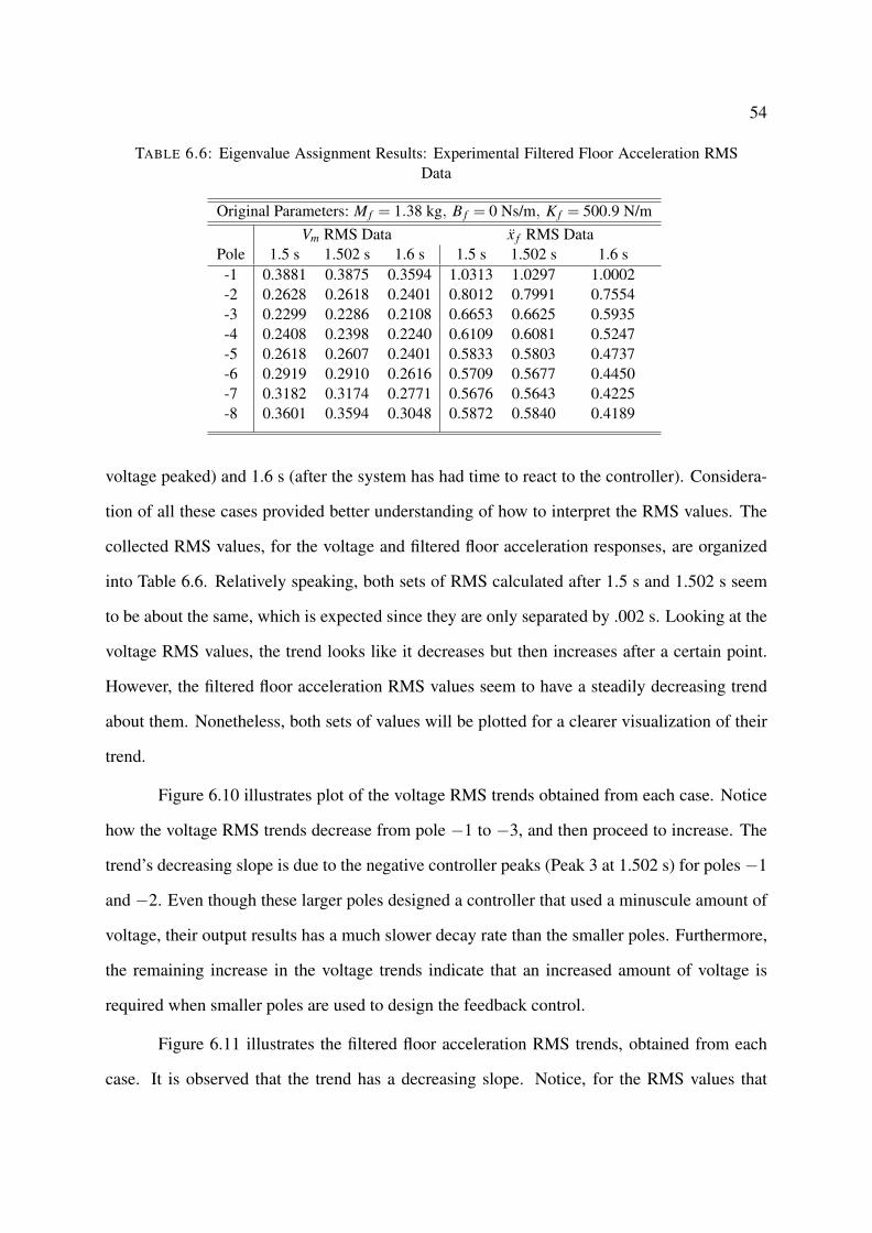
54

TABLE 6.6: Eigenvalue Assignment Results: Experimental Filtered Floor Acceleration RMSData

Original Parameters: M f = 1.38 kg, B f = 0 Ns/m, K f = 500.9 N/mVm RMS Data x f RMS Data

Pole 1.5 s 1.502 s 1.6 s 1.5 s 1.502 s 1.6 s-1 0.3881 0.3875 0.3594 1.0313 1.0297 1.0002-2 0.2628 0.2618 0.2401 0.8012 0.7991 0.7554-3 0.2299 0.2286 0.2108 0.6653 0.6625 0.5935-4 0.2408 0.2398 0.2240 0.6109 0.6081 0.5247-5 0.2618 0.2607 0.2401 0.5833 0.5803 0.4737-6 0.2919 0.2910 0.2616 0.5709 0.5677 0.4450-7 0.3182 0.3174 0.2771 0.5676 0.5643 0.4225-8 0.3601 0.3594 0.3048 0.5872 0.5840 0.4189

voltage peaked) and 1.6 s (after the system has had time to react to the controller). Considera-

tion of all these cases provided better understanding of how to interpret the RMS values. The

collected RMS values, for the voltage and filtered floor acceleration responses, are organized

into Table 6.6. Relatively speaking, both sets of RMS calculated after 1.5 s and 1.502 s seem

to be about the same, which is expected since they are only separated by .002 s. Looking at the

voltage RMS values, the trend looks like it decreases but then increases after a certain point.

However, the filtered floor acceleration RMS values seem to have a steadily decreasing trend

about them. Nonetheless, both sets of values will be plotted for a clearer visualization of their

trend.

Figure 6.10 illustrates plot of the voltage RMS trends obtained from each case. Notice

how the voltage RMS trends decrease from pole −1 to −3, and then proceed to increase. The

trend’s decreasing slope is due to the negative controller peaks (Peak 3 at 1.502 s) for poles −1

and −2. Even though these larger poles designed a controller that used a minuscule amount of

voltage, their output results has a much slower decay rate than the smaller poles. Furthermore,

the remaining increase in the voltage trends indicate that an increased amount of voltage is

required when smaller poles are used to design the feedback control.

Figure 6.11 illustrates the filtered floor acceleration RMS trends, obtained from each

case. It is observed that the trend has a decreasing slope. Notice, for the RMS values that

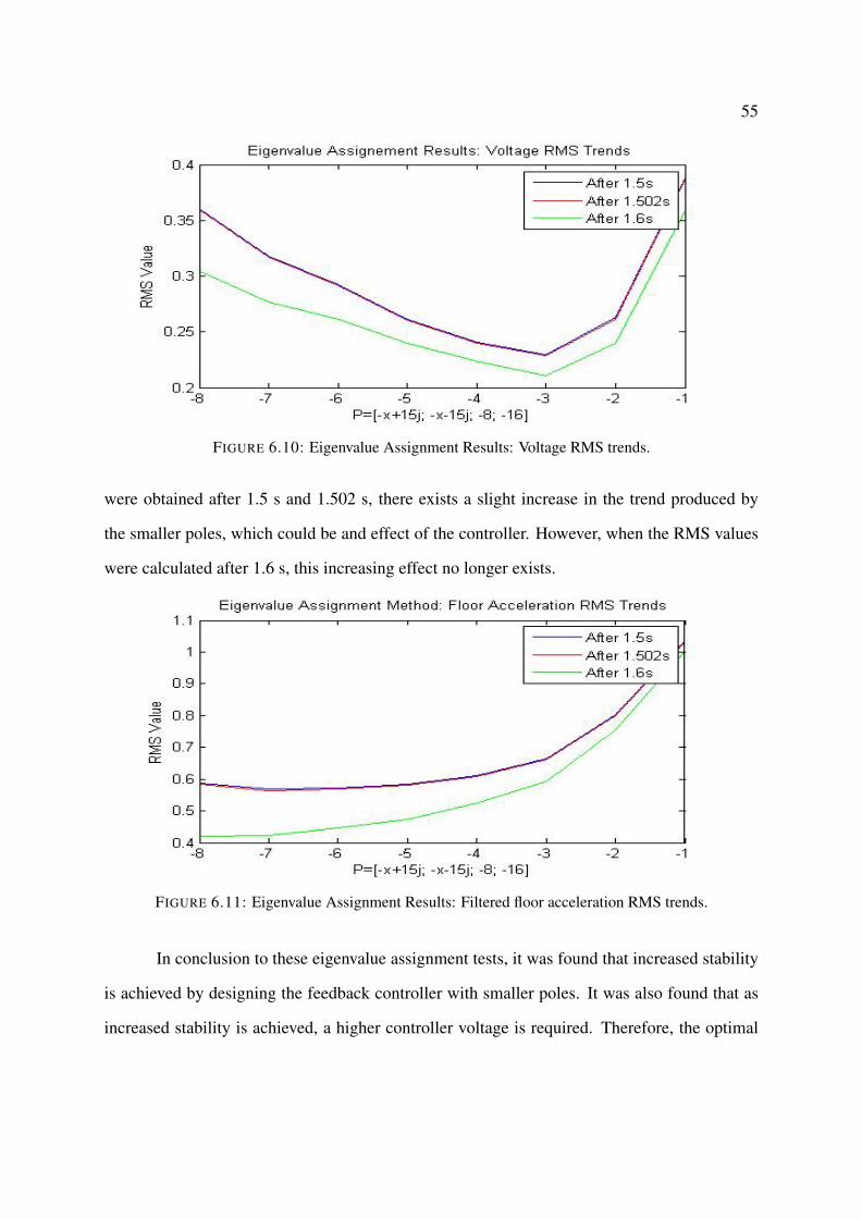
55

FIGURE 6.10: Eigenvalue Assignment Results: Voltage RMS trends.

were obtained after 1.5 s and 1.502 s, there exists a slight increase in the trend produced by

the smaller poles, which could be and effect of the controller. However, when the RMS values

were calculated after 1.6 s, this increasing effect no longer exists.

FIGURE 6.11: Eigenvalue Assignment Results: Filtered floor acceleration RMS trends.

In conclusion to these eigenvalue assignment tests, it was found that increased stability

is achieved by designing the feedback controller with smaller poles. It was also found that as

increased stability is achieved, a higher controller voltage is required. Therefore, the optimal

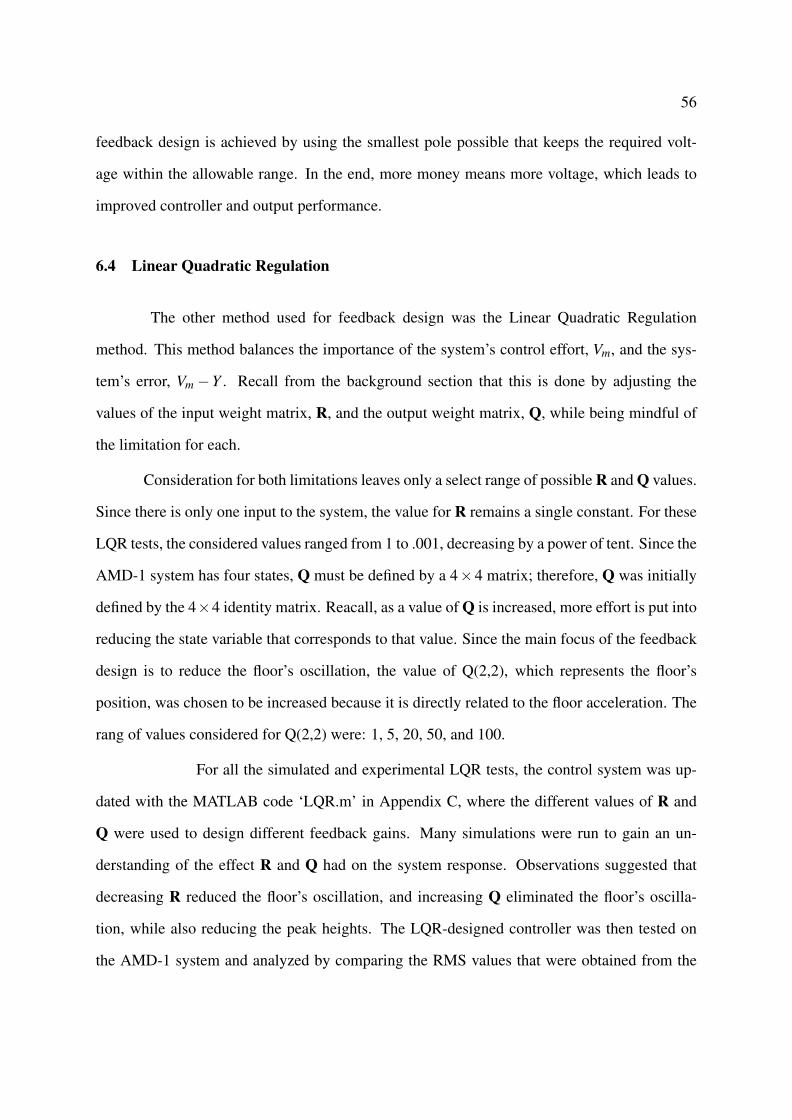
56

feedback design is achieved by using the smallest pole possible that keeps the required volt-

age within the allowable range. In the end, more money means more voltage, which leads to

improved controller and output performance.

6.4 Linear Quadratic Regulation

The other method used for feedback design was the Linear Quadratic Regulation

method. This method balances the importance of the system’s control effort, Vm, and the sys-

tem’s error, Vm−Y . Recall from the background section that this is done by adjusting the

values of the input weight matrix, R, and the output weight matrix, Q, while being mindful of

the limitation for each.

Consideration for both limitations leaves only a select range of possible R and Q values.

Since there is only one input to the system, the value for R remains a single constant. For these

LQR tests, the considered values ranged from 1 to .001, decreasing by a power of tent. Since the

AMD-1 system has four states, Q must be defined by a 4×4 matrix; therefore, Q was initially

defined by the 4×4 identity matrix. Reacall, as a value of Q is increased, more effort is put into

reducing the state variable that corresponds to that value. Since the main focus of the feedback

design is to reduce the floor’s oscillation, the value of Q(2,2), which represents the floor’s

position, was chosen to be increased because it is directly related to the floor acceleration. The

rang of values considered for Q(2,2) were: 1, 5, 20, 50, and 100.

For all the simulated and experimental LQR tests, the control system was up-

dated with the MATLAB code ‘LQR.m’ in Appendix C, where the different values of R and

Q were used to design different feedback gains. Many simulations were run to gain an un-

derstanding of the effect R and Q had on the system response. Observations suggested that

decreasing R reduced the floor’s oscillation, and increasing Q eliminated the floor’s oscilla-

tion, while also reducing the peak heights. The LQR-designed controller was then tested on

the AMD-1 system and analyzed by comparing the RMS values that were obtained from the

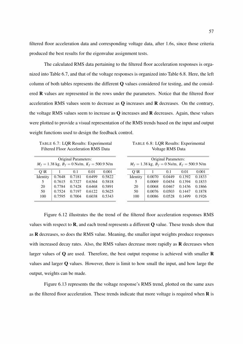
57

filtered floor acceleration data and corresponding voltage data, after 1.6s, since those criteria

produced the best results for the eigenvalue assignment tests.

The calculated RMS data pertaining to the filtered floor acceleration responses is orga-

nized into Table 6.7, and that of the voltage responses is organized into Table 6.8. Here, the left

column of both tables represents the different Q values considered for testing, and the consid-

ered R values are represented in the rows under the parameters. Notice that the filtered floor

acceleration RMS values seem to decrease as Q increases and R decreases. On the contrary,

the voltage RMS values seem to increase as Q increases and R decreases. Again, these values

were plotted to provide a visual representation of the RMS trends based on the input and output

weight functions used to design the feedback control.

TABLE 6.7: LQR Results: ExperimentalFiltered Floor Acceleration RMS Data

Original Parameters:M f = 1.38 kg, B f = 0 Ns/m, K f = 500.9 N/m

Q \R 1 0.1 0.01 0.001Identity 0.7648 0.7181 0.6499 0.5822

5 0.7615 0.7327 0.6364 0.581820 0.7784 0.7428 0.6468 0.589150 0.7524 0.7197 0.6122 0.5625

100 0.7595 0.7004 0.6038 0.5343

TABLE 6.8: LQR Results: ExperimentalVoltage RMS Data

Original Parameters:M f = 1.38 kg, B f = 0 Ns/m, K f = 500.9 N/m

Q \R 1 0.1 0.01 0.001Identity 0.0070 0.0449 0.1392 0.1833

5 0.0069 0.0454 0.1394 0.183320 0.0068 0.0467 0.1436 0.186650 0.0076 0.0503 0.1447 0.1878

100 0.0086 0.0528 0.1499 0.1926

Figure 6.12 illustrates the the trend of the filtered floor acceleration responses RMS

values with respect to R, and each trend represents a different Q value. These trends show that

as R decreases, so does the RMS value. Meaning, the smaller input weights produce responses

with increased decay rates. Also, the RMS values decrease more rapidly as R decreases when

larger values of Q are used. Therefore, the best output response is achieved with smaller R

values and larger Q values. However, there is limit to how small the input, and how large the

output, weights can be made.

Figure 6.13 represents the the voltage response’s RMS trend, plotted on the same axes

as the filtered floor acceleration. These trends indicate that more voltage is required when R is

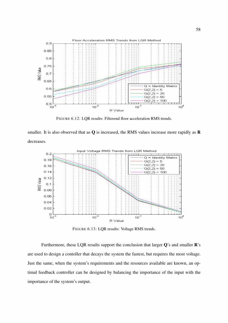
58

FIGURE 6.12: LQR results: Filterend floor acceleration RMS trends.

smaller. It is also observed that as Q is increased, the RMS values increase more rapidly as R

decreases.

FIGURE 6.13: LQR results: Voltage RMS trends.

Furthermore, these LQR results support the conclusion that larger Q’s and smaller R’s

are used to design a contoller that decays the system the fastest, but requires the most voltage.

Just the same, when the system’s requirements and the resources available are known, an op-

timal feedback controller can be designed by balancing the importance of the input with the

importance of the system’s output.

59

CHAPTER 7

CONCLUSION

This work presents an effective method for deriving the AMD-1 EOM, an improved

model of the AMD-1 system, and the design of a feedback control that successfully reduces

the oscillation of the AMD-1 structure upon excitation. The new derivation of the EOM used

the system’s free body diagram and its results were validated with Quanser’s EOM, which was

obtained from the Lagrange’s Method. This model was improved by considering the effect of

the structure’s viscous damping. The value of this damping coefficient, along with the corre-

sponding floor’s stiffness and mass, was determined through the force and motion sensor data

analysis.

Furthermore, two feedback design techniques were applied: eigenvalue assignment and

LQR. Analysis of both techniques were used to determine which method was more appropriate

and efficient. It was concluded that when the output’s primary focus is to satisfy the time-

domain specifications, then the eigenvalue assignment method is more effective. When the

output’s focus is to balance the importance of the control effort with the importance of reduced

vibration, then the LQR method becomes more effective.

7.1 Discussion

Simulated eigenvalue results indicated that the optimal floor acceleration responses

were obtained when the system’s feedback control was designed with the dominant pole’s that

were further from the stability boundary in the complex plane. However, the experimental

results, showed that little, to no, improvement was achieved once the poles moved past a certain

point. Comparison of the corresponding voltage responses showed that the demand for more

power increased more drastically as the dominant poles surpassed −6.

60

The LQR results indicated that the optimal response was achieved when Q(2,2) = 100

and R= .001, in other words, when Q was larger and R was smaller. This conclusion was made

from the RMS value trend analysis. Also, despite the fact that these Q and R values required

the highest amount of voltage out of all the LQR tests, comparison showed that there was no

alarming significance in the required voltage.

Furthermore, even though the feedback control that was designed in this work was made

specific to an AMD system, it could be applicable in any structure susceptible to wind or ground

excitation. As research continues, the efficiency and credibility of such a control system is sure

to grow, increasing the potential to save lives and preserve structures.

7.2 Future Research

Future research in this field could focus on the compensation for the presented sys-

tem’s limitations, or the derivation of a model that would reduce modeling error. Any time an

assumption is made, it increases the potential for error. When deriving the mathematical model

of the AMD-1 system, many parameters were neglected, or assumed to be negligible. Recall,

the nonlinear coulomb friction applied to the linear cart, the viscous damping force applied

to the floor, the friction between the cart and the structure, and the natural structure damping

were all neglected. In addition, the gravitational potential energy was assumed to be negligible.

Future research could develop a method that would include the loss due to these parameters or

verify their negligence.

With respect to resource availability, the accessibility to a larger power source and/or

higher accuracy amplifiers and sensors would guarantee the achievement of a higher degree of

stability. In addition, a method that would accurately estimate the system parameters (mass,

spring constant and damping coefficient) could be proposed, which would result in a even more

accurate model of the system.

61

It should also be considered that, in reality, the buildings and structures at the highest

risk have multiple degrees of freedom and their system parameters continually fluctuate over

time. A structure’s mass fluctuates daily as an effect of various personnel and merchandise

continually entering and leaving, and a structure’s stiffness and viscous damping fluctuates

over the years as an effect of aging and weathering. Therefore, some other ideal topics of study

would include the modeling of MIMO systems and the addition of an adaptation system that

would continuously estimate the system parameters and update the control system.

62

REFERENCES

[1] 4.5+ Magnitude Earthquakes since 1973. (n.d.). Google Fusion Tables. Retrieved March

4, 2014, from https://www.google.com/fusiontables/DataSource?dsrcid=579510.

[2] Agrawal, A. K., Yang, J. N., Schmitendorf, W. E., & Jabbari, F. (1997). Stability of Ac-

tively Controlled Structures with Actuator Saturation. Journal of Structural Engineering,

123(4), 505.

[3] Alkhatib, R., & Golnaraghi, M. F. (2003). Active Structural Vibration Control: A Review.

The Shock and Vibration Digest, 35(5), 367-383.

[4] Ashokkumar, C. R., & Iyengar, N. (2011). Partial Eigenvalue Assignment for Structural

Damage Mitigation. Journal of Sound and Vibration, 330(1), 9-16.

[5] Bdar, S., Prof. Shuyan, M., Saifullah, S., & Dr. Jie, H. (2013). Comparison of PID, Pole

Placement and LQR Controllers for Speed Ratio Control of Continuously Variable Trans-

mission (CVT). ICAMECE 2013, 149-153.

[6] Ding, Y. C., Weng, F. L., & Yu, Z. A. (2013). Actuator Saturation and Control Design for

Buildings Structural Systems with Improved Uncertainty Description. Shock and Vibra-

tion, 20(2), 297-308.

[7] Gajic, Z., & Lelic, M. (1996). Chapter 5: Controllability and Observability. Modern Con-

trol Systems Engineering. London: Prentice Hall.

[8] Guzzardo, C. A., (2012). Optimal Actuation in Active Vibration Control using Pole-

Placement. (Unpublished doctoral dissertation). Louisiana State University and Agricul-

tural and Mechanical College, Louisiana.

[9] Hanagan, L. M., & Murray, T. M. (1997). Active Control Approach for Reducing Floor

Vibrations. Journal of Structural Engineering, 123(11), 1497–1505.

63

[10] Hanagan, L. M., Kulasekere, E. C., Walgama, K. S., & Premaratne, K. (2000). Optimal

Placement of Actuators and Sensors for Floor Vibration Control. Journal of Structural

Engineering, 126(12), 1380-1387.

[11] Hochrainer, M. J. (2005). Tuned Liquid Column Damper for Structural Control. Acta

Mechanica, 175(1-4),57-76.

[12] Juang, J., & Maghami, P. G. (1990). Robust Eigensystem Assignment for Second-Order

Dynamic Systems. Mechanics and control of Large Flexible Structure, Progress in Astro-

nautics and Aeronautics, 129(14), 373-387.

[13] Junkins, J. L., & Kim, Y. (1990). Minimum Sensitivity Design Method for Output Feed-

back. Mechanics and Control of Large Flexible Structure, Progress in Astronautics and

Aeronautics, 129(15), 389-409.

[14] Kumar, R., & Khan, M. (2007). Pole Placement Techniques for Active Vibration Control

of Smart Structures: A Feasibility Study. Journal of Vibration and Acoustics, 129(5),

601-615.

[15] Landau, I. D., Lozano, R., M’Saad, M., & Karimi, A. (2011). Adaptive control algorithms,

analysis and applications (2nd ed.). London: Springer.

[16] Lin, Y. K., & Yong, Y. (1987). Evolutionary Kanai-Tajimi Type Earthquake Models. Jour-

nal of Engineering Mechanics, 113(8).

[17] Luca, S. G, Chira, F., & Rosca, V. O. (2005). Passive, Active and Semi-Active Control

Systems in Civil Engineering. Tomul LI (LV), Fasc. 3(4) 23-31.

[18] Manufacturing Education 1998. Free decay curve. [Plot]. Retrived from

http://www.mfg.mtu.edu/marc/primers/machtool/vibration/damping.html

[19] Marinova, D., & Marinov, V. (2005). Numerical Design of Optimal Active Control for

Seismically-Excited Building Structures. Numerical Analysis and Its Applications: Third

64

International Conference, NAA 2004, Rousse, Bulgaria, June 29-July 3, 2004: Revised

Selected Papers, Berlin: Springer, 408-415.

[20] Maurer Sohnoe - Innovation in Steel. (Since, 1876). Maurer Tuned Mass Dampers - Tech-

nical Information and Products. Retrieved May. 19, 2014,

[21] Meadows, H. E. (2006). Controllability and Observability in Time-Variable Linear Sys-

tems. SIAM Journal on Control, 5, 64-73.

[22] Munich Re. n.d. Leading natural disasters, by overall economic losses, since 1980. [Map].

Retrieved from http://www.economist.com/node/21542755

[23] Mei, G., Kareem, A., & Kantor, J. C. (2001). Real-Time Model Predictive Control of

Structures under Earthquakes. Earthquake Engineering & Structural Dynamics, 30(7),

995-1019.

[24] Mei, G., Kareem, A., & Kantor, J. C. (2002). Model Predictive Control of Structures Un-

der Earthquakes using Acceleration Feedback. Journal of Engineering Mechanics, 128(5),

574.

[25] No Author. Linear-Quadratic Regulator (LQR) Design. (2014, January 1). Retrieved June

2, 2014, from http://www.mathworks.com

[26] No Last Name, James. 2011. Worldwide map of nuclear power stations and earth-

quake zones. [Map]. Retrieved from http://maptd.com/worldwide-map-of-nuclear-power-

stations-and-earthquake-zones/

[27] Nuclear Power Stations Worldwide. (n.d.). Google Fusion Tables. Retrieved March 4,

2014, from https://www.google.com/fusiontables/DataSource?dsrcid=579353

[28] Ouyang, H., & Singh, K. V. (2010). Pole Assignment for Asymmetric Systems Using

State- feedback with Time Delay. Active Vibration Control, Proceedings of ISMA2010

Including USD2010, 383-390.

65

[29] Quanser. Active Mass Damper - One Floor. Linear Experiment #9: Vibration control,

1-19.

[30] Robinson, J. K., Gamble, S. L., & Myslimaj, B. M. (2007, June) Supplemental Damping

and Using Tuned Sloshing Dampers. STRUCTURE Magazine: Practical Solutions - Real

World Solutions for the Practicing Structural Engineer, 14-18.

[31] Sakai, H., & Arase, M. (1979). Recursive Parameter Estimation of an Autoregressive

Process Disturbed by White Noise. International Journal of Control, 30(6), 949-966.

[32] Scheller, J., & Starossek, U. (2011). A versatile active mass damper for structural vibra-

tion control. Proceedings of the 8th International Conference on Structural Dynamics,

EURODYN 2011: Leuven, Belgium, 4-6 July 2011, S.I: s.n.j., 1777-1784.

[33] Sivanadyan, T., & Sayeed, A. (2006). Active Wireless Sensing for Rapid Information

Retrieval in Sensor Networks, Information Processing in Sensor Networks, IPSN 2006.

The Fifth International Conference, 85-92.

[34] Slater, G. L., & Zhang, Q. (1990). Controller Design by Eigenspace Assignment. Mechan-

ics and Control of Large Flexible Structure, Progress in Astronautics and Aeronautics,

129(17), 435-462.

[35] Tinkir, M., Kalyoncu, M., & Sahin, Y. (2013). Experimental Investigation of Full-Order

Observer and LQR Controlled Building-Like Structure Under Seismic Excitation. Applied

Mechanics and Materials, 307, 316-320.

[36] Watakabe, M., Chiba, O., & Kamada, T. (2004). Vibration Control of a Large-scale Test

Building using Hybrid Mass Damper System Applied Robust Control Theory. 13th World

Conference on Earthquake Engineering Vancouver, B.C., Canada August 1-6, 2004.

66

[37] Willis, A. G., Bates, D., Fleming, A. J., Ninness, B., & Moheimani, S. O. (2008). Model

Predictive Control Applied to Constraint Handling in Active Noise and Vibration Control.

IEEE Transactions on Control Systems Technology, 16(1), 3-12.

[38] Yamamoto, M., Aizawa, S., Higashino, M., & Toyama, K. (2001). Practical Applications

of Active Mass Dampers with Hydraulic Actuator. Earthquake Engineering & Structural

Dynamics, 30(11), 1697-1717.

[39] Yamamoto, M., & Sone, T. (2013). Behavior of active mass damper (AMD) Installed in

High-Rise Building During 2011 Earthquake off Pacific Coast of Tohoku and Verification

of Regenerating System of AMD Based on Monitoring. Structural Control and Health

Monitoring. 1.

[40] Zahrai, S.M., & Shafieezadeh, A. (2009). Semi-Active Control of the Wind-Excited

Benchmark Tall Building using a Fuzzy Controller. Iranian Journal of Science & Tech-

nology, Transaction B, Engineering, 33(B1), 1-14.

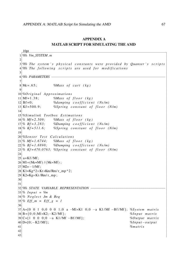
APPENDIX A: MATLAB Script for Simulating the AMD 67

APPENDIX AMATLAB SCRIPT FOR SIMULATING THE AMD

10pt1 %% Vm_SYSTEM .m23 %% The sys tem ’ s p h y s i c a l c o n s t a n t s were p r o v i d e d by Quanser ’ s s c r i p t s4 %% The f o l l o w i n g s c r i p t s are used f o r m o d i f i c a t i o n s56 %% PARAMETERS −−−−−−−−−−−−−−−−−−−−−−−−−−−−−−−−−−−−−−−−−−−−−−−−−−−−−−−78 Mc= . 6 5 ; %Mass o f c a r t ( kg )9

10 %O r i g i n a l A p p r o x i m a t i o n s11 Mf = 1 . 3 8 ; %Mass o f f l o o r ( kg )12 Bf =0; %damping c o e f f i c i e n t ( Ns /m)13 Kf = 5 0 0 . 9 ; %S p r i n g c o n s t a n t o f f l o o r (N /m)1415 %S i m u l i n k Toolbox E s t i m a t i o n s16 % Mf =2.509; %Mass o f f l o o r ( kg )17 % Bf =3.283; %Damping c o e f f i c i e n t ( Ns /m)18 % Kf =511 .6 ; %S p r i n g c o n s t a n t o f f l o o r (N /m)1920 %Se ns or T e s t C a l c u l a t i o n s21 % Mf =1.6744; %Mass o f f l o o r ( kg )22 % Bf =1.8898; %Damping c o e f f i c i e n t ( Ns /m)23 % Kf =470.0763; %S p r i n g c o n s t a n t o f f l o o r (N /m)2425 a=Kf / Mf ;26 M1=(Mc+Mf ) / ( Mc∗Mf ) ;27 M2=−1/Mf ;28 K1=Kg^2∗Kt∗Km/Rm/ r_mp ^ 2 ;29 K2=Kg∗Kt /Rm/ r_mp ;303132 %% STATE VARIABLE REPRESENTATION −−−−−−−−−−−−−−−−−−−−−−−−−−−−−−−−−−−−33 % I n p u t = Vm34 % N e g l e c t Jm & Beq35 % Eff_m = E f f _ g = 13637 A=[0 0 1 0 ; 0 0 0 1 ; 0 a −M1∗K1 0 ; 0 −a K1 / Mf −Bf / Mf ] ; %Sys tem m a t r i x38 B = [ 0 ; 0 ;M1∗K2;−K2 / Mf ] ; %I n p u t m a t r i x39 C=[1 0 0 0 ; 0 −a K1 / Mf −Bf / Mf ] ; %Outpu t m a t r i x40 D=[0;−K2 / Mf ] ; %I n p u t−o u t p u t41 %m a t r i x4243

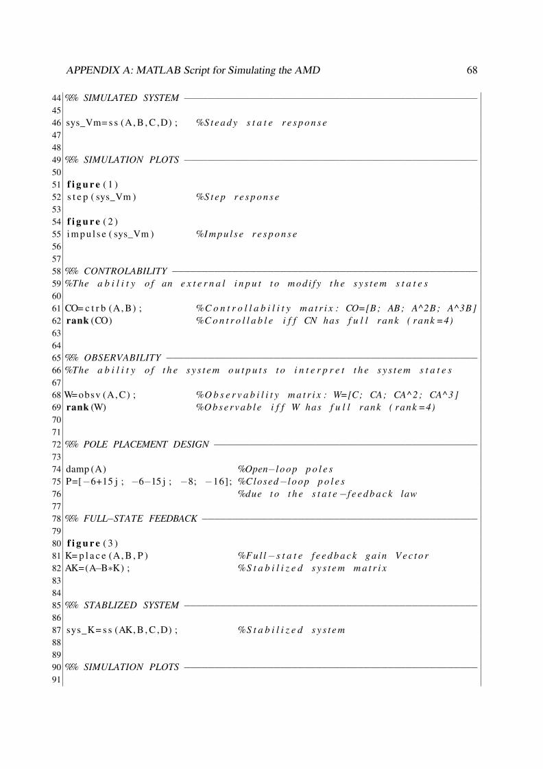
APPENDIX A: MATLAB Script for Simulating the AMD 68

44 %% SIMULATED SYSTEM −−−−−−−−−−−−−−−−−−−−−−−−−−−−−−−−−−−−−−−−−−−−−−−−−4546 sys_Vm= s s (A, B , C ,D) ; %S t e a d y s t a t e r e s p o n s e474849 %% SIMULATION PLOTS −−−−−−−−−−−−−−−−−−−−−−−−−−−−−−−−−−−−−−−−−−−−−−−−−5051 f i g u r e ( 1 )52 s t e p ( sys_Vm ) %S t e p r e s p o n s e5354 f i g u r e ( 2 )55 i m p u l s e ( sys_Vm ) %I m p u l s e r e s p o n s e565758 %% CONTROLABILITY −−−−−−−−−−−−−−−−−−−−−−−−−−−−−−−−−−−−−−−−−−−−−−−−−−−59 %The a b i l i t y o f an e x t e r n a l i n p u t t o m od i f y t h e s y s t e m s t a t e s6061 CO= c t r b (A, B) ; %C o n t r o l l a b i l i t y m a t r i x : CO=[B ; AB ; A^2B ; A^3B]62 rank (CO) %C o n t r o l l a b l e i f f CN has f u l l rank ( rank =4)636465 %% OBSERVABILITY −−−−−−−−−−−−−−−−−−−−−−−−−−−−−−−−−−−−−−−−−−−−−−−−−−−−66 %The a b i l i t y o f t h e s y s t e m o u t p u t s t o i n t e r p r e t t h e s y s t e m s t a t e s6768 W=obsv (A, C) ; %O b s e r v a b i l i t y m a t r i x : W=[C; CA; CA^ 2 ; CA^3]69 rank (W) %O b s e r v a b l e i f f W has f u l l rank ( rank =4)707172 %% POLE PLACEMENT DESIGN −−−−−−−−−−−−−−−−−−−−−−−−−−−−−−−−−−−−−−−−−−−−7374 damp (A) %Open−l oop p o l e s75 P=[−6+15 j ; −6−15 j ; −8; −16]; %Closed−l oop p o l e s76 %due t o t h e s t a t e−f e e d b a c k law7778 %% FULL−STATE FEEDBACK −−−−−−−−−−−−−−−−−−−−−−−−−−−−−−−−−−−−−−−−−−−−−−7980 f i g u r e ( 3 )81 K= p l a c e (A, B , P ) %Ful l−s t a t e f e e d b a c k ga in V e c t o r82 AK=(A−B∗K) ; %S t a b i l i z e d s y s t e m m a t r i x838485 %% STABLIZED SYSTEM −−−−−−−−−−−−−−−−−−−−−−−−−−−−−−−−−−−−−−−−−−−−−−−−−8687 sys_K= s s (AK, B , C ,D) ; %S t a b i l i z e d s y s t e m888990 %% SIMULATION PLOTS −−−−−−−−−−−−−−−−−−−−−−−−−−−−−−−−−−−−−−−−−−−−−−−−−91

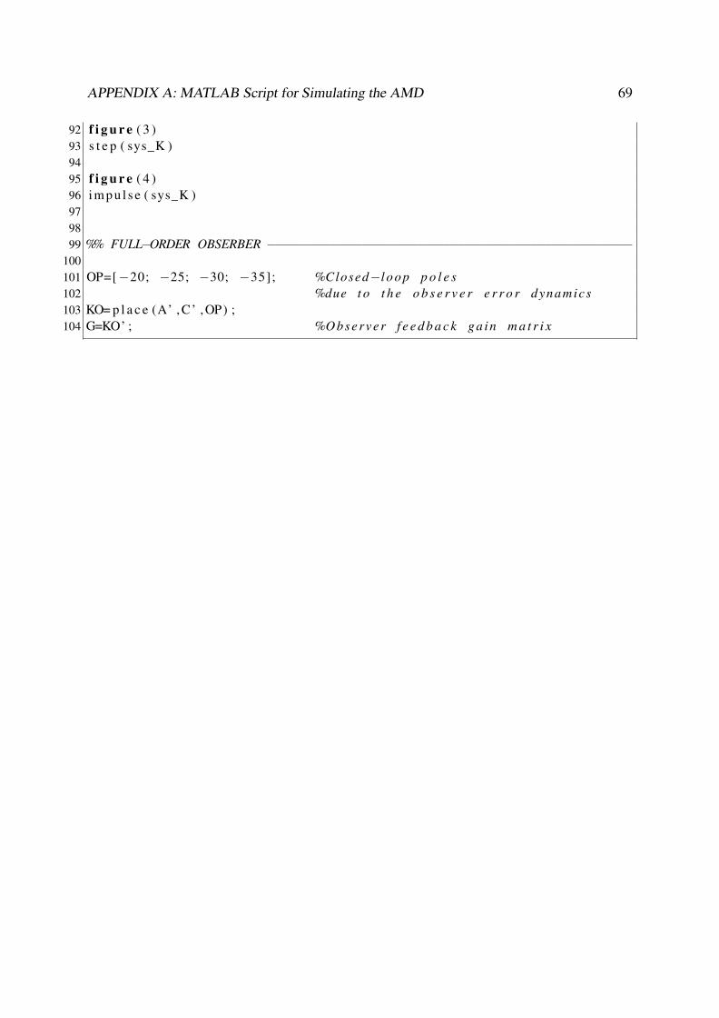
APPENDIX A: MATLAB Script for Simulating the AMD 69

92 f i g u r e ( 3 )93 s t e p ( sys_K )9495 f i g u r e ( 4 )96 i m p u l s e ( sys_K )979899 %% FULL−ORDER OBSERBER −−−−−−−−−−−−−−−−−−−−−−−−−−−−−−−−−−−−−−−−−−−−−−

100101 OP=[−20; −25; −30; −35]; %Closed−l oop p o l e s102 %due t o t h e o b s e r v e r e r r o r dynamics103 KO= p l a c e (A’ , C’ , OP) ;104 G=KO’ ; %Observer f e e d b a c k ga in m a t r i x

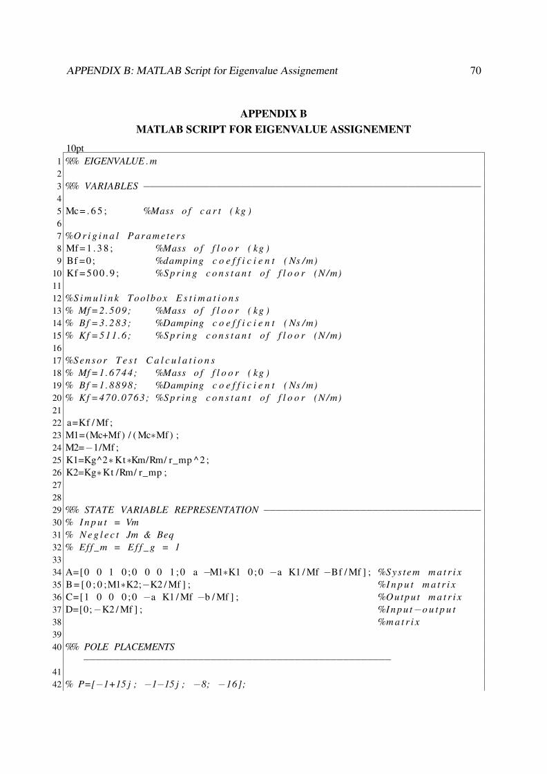
APPENDIX B: MATLAB Script for Eigenvalue Assignement 70

APPENDIX BMATLAB SCRIPT FOR EIGENVALUE ASSIGNEMENT

10pt1 %% EIGENVALUE .m23 %% VARIABLES −−−−−−−−−−−−−−−−−−−−−−−−−−−−−−−−−−−−−−−−−−−−−−−−−−−−−−−−45 Mc= . 6 5 ; %Mass o f c a r t ( kg )67 %O r i g i n a l Parame ter s8 Mf = 1 . 3 8 ; %Mass o f f l o o r ( kg )9 Bf =0; %damping c o e f f i c i e n t ( Ns /m)

10 Kf = 5 0 0 . 9 ; %S p r i n g c o n s t a n t o f f l o o r (N /m)1112 %S i m u l i n k Toolbox E s t i m a t i o n s13 % Mf =2.509; %Mass o f f l o o r ( kg )14 % Bf =3.283; %Damping c o e f f i c i e n t ( Ns /m)15 % Kf =511 .6 ; %S p r i n g c o n s t a n t o f f l o o r (N /m)1617 %Se ns or T e s t C a l c u l a t i o n s18 % Mf =1.6744; %Mass o f f l o o r ( kg )19 % Bf =1.8898; %Damping c o e f f i c i e n t ( Ns /m)20 % Kf =470.0763; %S p r i n g c o n s t a n t o f f l o o r (N /m)2122 a=Kf / Mf ;23 M1=(Mc+Mf ) / ( Mc∗Mf ) ;24 M2=−1/Mf ;25 K1=Kg^2∗Kt∗Km/Rm/ r_mp ^ 2 ;26 K2=Kg∗Kt /Rm/ r_mp ;272829 %% STATE VARIABLE REPRESENTATION −−−−−−−−−−−−−−−−−−−−−−−−−−−−−−−−−−−−30 % I n p u t = Vm31 % N e g l e c t Jm & Beq32 % Eff_m = E f f _ g = 13334 A=[0 0 1 0 ; 0 0 0 1 ; 0 a −M1∗K1 0 ; 0 −a K1 / Mf −Bf / Mf ] ; %Sys tem m a t r i x35 B = [ 0 ; 0 ;M1∗K2;−K2 / Mf ] ; %I n p u t m a t r i x36 C=[1 0 0 0 ; 0 −a K1 / Mf −b / Mf ] ; %Outpu t m a t r i x37 D=[0;−K2 / Mf ] ; %I n p u t−o u t p u t38 %m a t r i x3940 %% POLE PLACEMENTS

−−−−−−−−−−−−−−−−−−−−−−−−−−−−−−−−−−−−−−−−−−−−−−−−−−−4142 % P=[−1+15 j ; −1−15 j ; −8; −16];

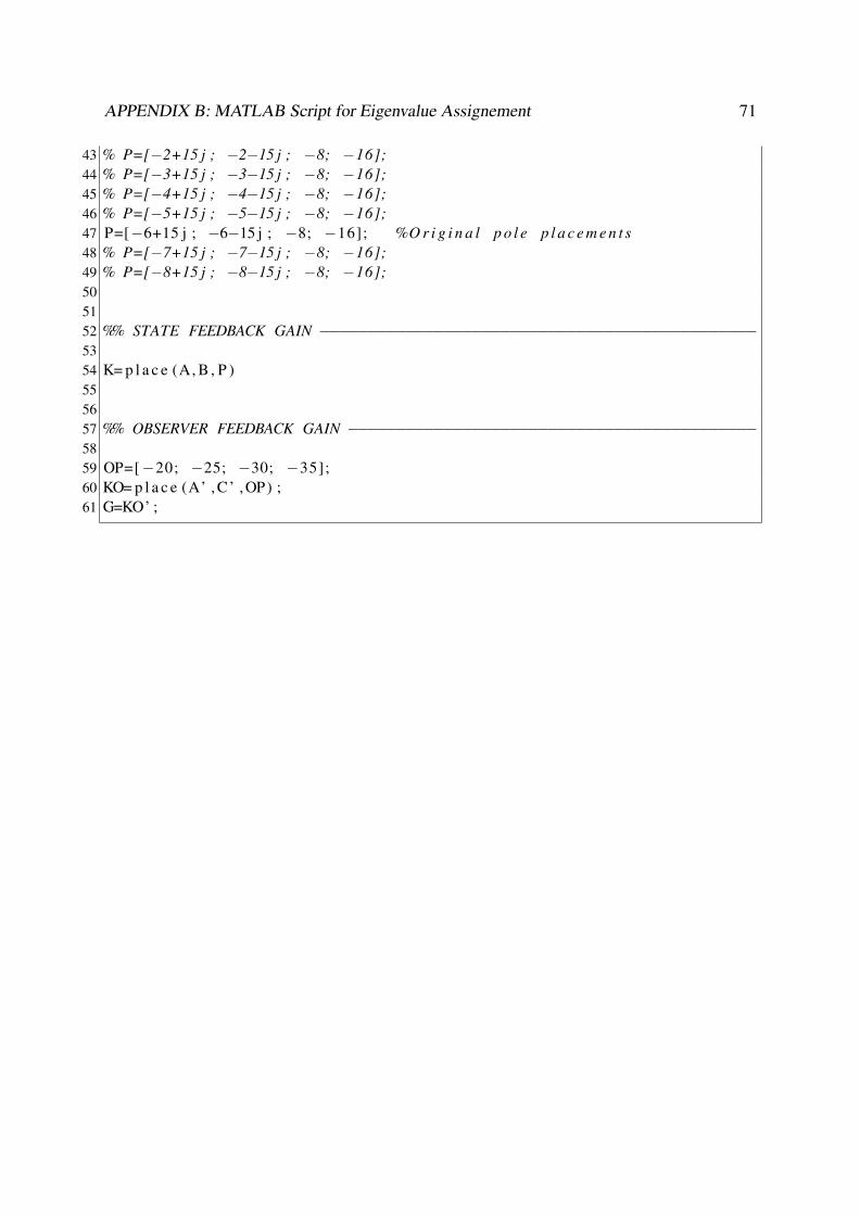
APPENDIX B: MATLAB Script for Eigenvalue Assignement 71

43 % P=[−2+15 j ; −2−15 j ; −8; −16];44 % P=[−3+15 j ; −3−15 j ; −8; −16];45 % P=[−4+15 j ; −4−15 j ; −8; −16];46 % P=[−5+15 j ; −5−15 j ; −8; −16];47 P=[−6+15 j ; −6−15 j ; −8; −16]; %O r i g i n a l p o l e p l a c e m e n t s48 % P=[−7+15 j ; −7−15 j ; −8; −16];49 % P=[−8+15 j ; −8−15 j ; −8; −16];505152 %% STATE FEEDBACK GAIN −−−−−−−−−−−−−−−−−−−−−−−−−−−−−−−−−−−−−−−−−−−−−−5354 K= p l a c e (A, B , P )555657 %% OBSERVER FEEDBACK GAIN −−−−−−−−−−−−−−−−−−−−−−−−−−−−−−−−−−−−−−−−−−−5859 OP=[−20; −25; −30; −35];60 KO= p l a c e (A’ , C’ , OP) ;61 G=KO’ ;

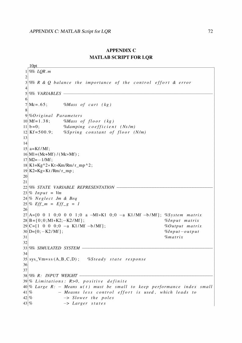
APPENDIX C: MATLAB Script for LQR 72

APPENDIX CMATLAB SCRIPT FOR LQR

10pt1 %% LQR .m23 %% R & Q b a l a n c e t h e i m p o r t a n c e o f t h e c o n t r o l e f f o r t & e r r o r45 %% VARIABLES −−−−−−−−−−−−−−−−−−−−−−−−−−−−−−−−−−−−−−−−−−−−−−−−−−−−−−−−67 Mc= . 6 5 ; %Mass o f c a r t ( kg )89 %O r i g i n a l Parame ter s

10 Mf = 1 . 3 8 ; %Mass o f f l o o r ( kg )11 b =0; %damping c o e f f i c i e n t ( Ns /m)12 Kf = 5 0 0 . 9 ; %S p r i n g c o n s t a n t o f f l o o r (N /m)131415 a=Kf / Mf ;16 M1=(Mc+Mf ) / ( Mc∗Mf ) ;17 M2=−1/Mf ;18 K1=Kg^2∗Kt∗Km/Rm/ r_mp ^ 2 ;19 K2=Kg∗Kt /Rm/ r_mp ;202122 %% STATE VARIABLE REPRESENTATION −−−−−−−−−−−−−−−−−−−−−−−−−−−−−−−−−−−−23 % I n p u t = Vm24 % N e g l e c t Jm & Beq25 % Eff_m = E f f _ g = 12627 A=[0 0 1 0 ; 0 0 0 1 ; 0 a −M1∗K1 0 ; 0 −a K1 / Mf −b / Mf ] ; %Sys tem m a t r i x28 B = [ 0 ; 0 ;M1∗K2;−K2 / Mf ] ; %I n p u t m a t r i x29 C=[1 0 0 0 ; 0 −a K1 / Mf −b / Mf ] ; %Outpu t m a t r i x30 D=[0;−K2 / Mf ] ; %I n p u t−o u t p u t31 %m a t r i x3233 %% SIMULATED SYSTEM −−−−−−−−−−−−−−−−−−−−−−−−−−−−−−−−−−−−−−−−−−−−−−−−−3435 sys_Vm= s s (A, B , C ,D) ; %S t e a d y s t a t e r e s p o n s e363738 %% R : INPUT WEIGHT −−−−−−−−−−−−−−−−−−−−−−−−−−−−−−−−−−−−−−−−−−−−−−−−−−39 % L i m i t a t i o n s : R>0 , p o s i t i v e d e f i n i t e40 % Large R : − Means u ( t ) must be s m a l l t o keep per fo rmance i n d e x s m a l l41 % − Measns l e s s c o n t r o l e f f o r t i s used , which l e a d s t o42 % −> Slower t h e p o l e s43 % −> Larger s t a t e s

APPENDIX C: MATLAB Script for LQR 73

4445 R=1;46 % R= . 1 ;47 % R=.01 ;48 % R=.001;495051 %% Q: OUTPUT WEIGHT −−−−−−−−−−−−−−−−−−−−−−−−−−−−−−−−−−−−−−−−−−−−−−−−−52 % L i m i t a t i o n s : Q−NR^(−1)N’ >0 , p o s i t i v e semi−d e f i n i t e53 % Large Q: − Means x ( t ) must be s m a l l t o keep per fo rmance i n d e x s m a l l5455 %S t a r t w i t h Q=eye ( 4 )56 Q=eye ( 4 ) ;5758 %I n c r e a s e v a l u e s c o r r e s p o n d i n g t o t h e s t a t e s you want t o p u t more59 %e f f o r t i n t o k e e p i n g s m a l l .60 % Q( 2 , 2 ) =5;61 % Q( 2 , 2 ) =10;62 % Q( 2 , 2 ) =20;63 % Q( 2 , 2 ) =50;64 Q( 2 , 2 ) =100;656667 %% STATE FEEDBACK GAIN −−−−−−−−−−−−−−−−−−−−−−−−−−−−−−−−−−−−−−−−−−−−−−6869 KL= l q r (A, B , Q, R) %LQR f e e d b a c k ga in70 AL=(A−B∗KL) ; %LQR s y s t e m m a t r i x7172 K=KL737475 %% SIMULATED SYSTEM −−−−−−−−−−−−−−−−−−−−−−−−−−−−−−−−−−−−−−−−−−−−−−−−−7677 sys_L= s s (AL, B , C ,D) ;7879 %% SIMULATION PLOTS −−−−−−−−−−−−−−−−−−−−−−−−−−−−−−−−−−−−−−−−−−−−−−−−−8081 f i g u r e ( 1 )82 s t e p ( sys_L )8384 f i g u r e ( 2 )85 i m p u l s e ( sys_L )

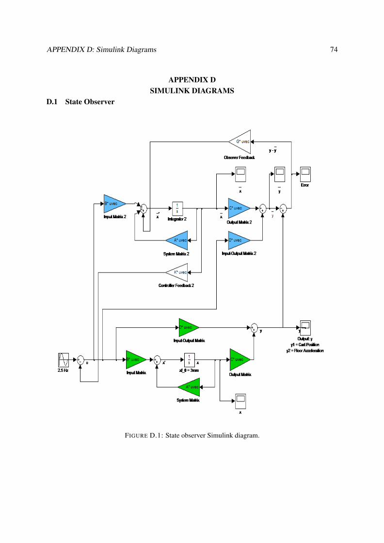
APPENDIX D: Simulink Diagrams 74

APPENDIX DSIMULINK DIAGRAMS

D.1 State Observer

FIGURE D.1: State observer Simulink diagram.

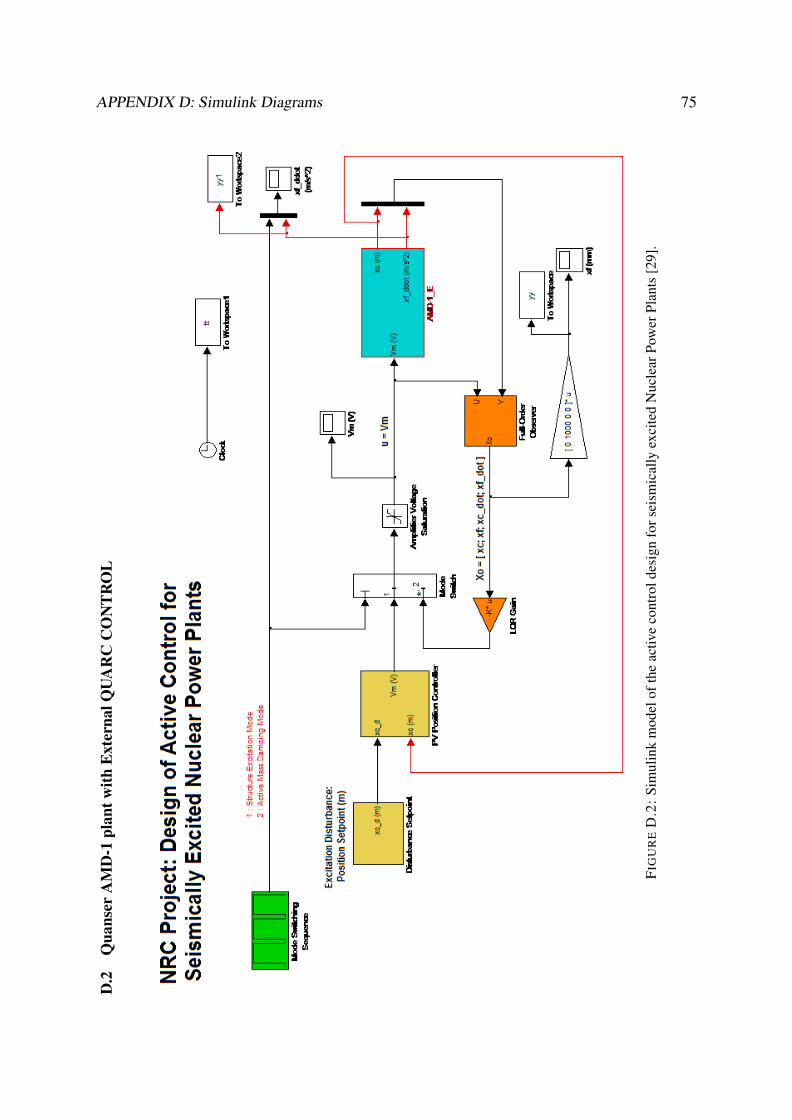
APPENDIX D: Simulink Diagrams 75D

.2Q

uans

erA

MD

-1pl

antw

ithE

xter

nalQ

UA

RC

CO

NT

RO

L

FIG

UR

ED

.2:

Sim

ulin

km

odel

ofth

eac

tive

cont

rold

esig

nfo

rsei

smic

ally

exci

ted

Nuc

lear

Pow

erPl

ants

[29]

.