Embed Size (px)
Citation preview

The Pennsylvania State University
The Graduate School
Department of Mechanical Engineering
DESIGN OF HORIZONTAL CURVES WITH DOWNGRADES USING LOW-ORDER
VEHICLE DYNAMICS MODELS
A Thesis in
Mechanical Engineering
by
Tejas Varunjikar
2011 Tejas Varunjikar
Submitted in Partial Fulfillment
of the Requirements
for the Degree of
Master of Science
May 2011

The thesis of Tejas Varunjikar was reviewed and approved* by the following:
Sean Brennan
Associate Professor, Department of Mechanical Engineering
Thesis Advisor
H. J. Sommer III
Professor, Department of Mechanical Engineering
Thesis Reader
Karen A. Thole
Professor, Department of Mechanical Engineering
Head of the Department of Mechanical Engineering
*Signatures are on file in the Graduate School

iii
ABSTRACT
Geometric design of highways is an important aspect of highway engineering, and in
particular, horizontal curves on highways have higher accident rates compared to straight roads.
Quantitative guidelines for horizontal curve design exist only for flat roads, but not downgrades.
This study uses a friction demand versus friction supply approach to check whether the current
horizontal curve design policies are acceptable for downgrades. Skid measurements combined
with a physics-based tire model are used to obtain the friction supply at various design speeds.
This thesis develops analytical as well as low-order simulation-based models for a vehicle
traveling on downgrade in order to find the friction demand of the vehicle. Results show that per-
axle friction demand can be significantly higher compared to the overall friction demand which is
basis of current design guidelines. The margins of safety are shown to significantly decrease with
design speed, and in the case of even moderate braking, go to a very low value at high speeds.

iv
TABLE OF CONTENTS
LIST OF FIGURES .................................................................................................. vi LIST OF TABLES ................................................................................................... x
Chapter 1 Introduction ............................................................................................................ 1
1.1 AASHTO Policy ........................................................................................................ 3 1.2 Motivation .................................................................................................................. 6 1.3 Proposed Vehicles Models ......................................................................................... 8 1.4 Thesis Overview ........................................................................................................ 10 References ........................................................................................................................ 11
Chapter 2 Literature Review ................................................................................................... 13
2.1 AASHTO Design Friction Factor .............................................................................. 13 2.2 Tire Pavement Friction Studies .................................................................................. 19 2.3 Friction Ellipse ........................................................................................................... 26 2.4 Tire Models ................................................................................................................ 29 2.5 Vehicle Dynamic Models ........................................................................................... 33
2.5.1 Two-axle Vehicle Models ............................................................................... 33 2.5.2 Bicycle Model Instabilities .............................................................................. 37 2.5.3 Multi-body Models .......................................................................................... 42
References ........................................................................................................................ 43
Chapter 3 Design Space and Tire-Pavement Friction Model .................................................. 46
3.1 Methodology .............................................................................................................. 46 3.2 Design Variables ........................................................................................................ 48 3.3 Vehicle Family ........................................................................................................... 52 3.4 Tire-Pavement Friction Model ................................................................................... 53 References ........................................................................................................................ 57
Chapter 4 Modified Point Mass Model and Static Rollover Model ........................................ 58
4.1 Coordinate System ..................................................................................................... 58 4.2 Equation of Motion .................................................................................................... 60 4.3 Friction Curves ........................................................................................................... 63 4.4 Static Rollover Model ................................................................................................ 68 References ........................................................................................................................ 72
Chapter 5 Steady-State Bicycle Model for 3D Terrain ........................................................... 73
5.1 Coordinate Transformations ....................................................................................... 74 5.2 Model Terminology ................................................................................................... 76 5.3 Equation of Motion .................................................................................................... 77 5.4 Brake Proportioning Model........................................................................................ 82 5.5 Friction Curves ........................................................................................................... 85 References ........................................................................................................................ 89

v
Chapter 6 Modified Transient Bicycle Model for 3D Terrain ................................................ 90
6.1 Coordinate Transformations ....................................................................................... 91 6.2 Equation of Motion .................................................................................................... 92 6.3 Extension using Linear Tire Model ............................................................................ 95 6.4 Vehicle Maneuver ...................................................................................................... 97 6.5 Friction Curves ........................................................................................................... 101 6.6 Lane Change Maneuver ............................................................................................. 104 References ........................................................................................................................ 108
Chapter 7 Multi-Body Simulations ......................................................................................... 109
7.1 CarSim Simulation Methodology .............................................................................. 109 7.1.1 Vehicle Assembly ........................................................................................... 110 7.1.2 3D Road .......................................................................................................... 111 7.1.3 Driver Path Follower ....................................................................................... 111 7.1.4 Speed Control .................................................................................................. 112
7.2 CarSim Simulation Comparison ................................................................................ 113 References ........................................................................................................................ 116
Chapter 8 Conclusions and Future Work ................................................................................ 117
8.1 Conclusions ................................................................................................................ 117 8.2 Future Work ............................................................................................................... 120
8.2.1 Tire-pavement friction ..................................................................................... 120 8.2.2 Crash Data Analysis ........................................................................................ 121 8.2.3 Road Geometries ............................................................................................. 122 8.2.4 Speed Studies .................................................................................................. 122 8.2.5 Heavy Vehicles ............................................................................................... 123 8.2.6 Low-Order Rollover Model ............................................................................ 123
References ........................................................................................................................ 124
Appendix A Glossary of Terms .............................................................................................. 125
Appendix B Vehicle Family Parameters ................................................................................. 130
vi
LIST OF FIGURES
Figure 1: Fatal crashes per year in the United States ([2]) ....................................................... 1
Figure 2: Percentage of fatalities by roadway alignment in 2002 ([3]) ................................... 2
Figure 3: A vehicle traveling on a superelevated road ............................................................. 3
Figure 4: Tire forces defining the (side) friction factor ([6]) ................................................... 4
Figure 5: AASHTO recommendation for design side friction factor vs. speed ([5]) ............... 5
Figure 6: Time response of a vehicle to a step steering input (CarSim simulation) ................ 8
Figure 7: Ball bank indicator ................................................................................................... 14
Figure 8: Ball bank indicator setup ([1]) .................................................................................. 14
Figure 9: Summary of various side friction studies ([1]) ......................................................... 17
Figure 10: Relationship between side friction demand and speed ([7]) ................................... 18
Figure 11: AASHTO recommendation for design side friction factor vs. speed ([1]) ............. 19
Figure 12: Relation between static, side skid and straight skid coefficients of friction on
wet Portland cement concrete ([4]) .................................................................................. 20
Figure 13: Side forces and brake forces generated by a tire ([12]) .......................................... 23
Figure 14: Effect of the speed on the coefficient of road adhesion ([11]) ............................... 23
Figure 15: Hydroplaning of a tire on flooded surfaces ([19]) .................................................. 24
Figure 16: Effect of tread design and surface conditions on the degradation of cornering
capability of tires on wet surfaces ([16]) .......................................................................... 25
Figure 17: Skid measurements vs. speed using ribbed tires on asphalt surface ([32]) ............ 26
Figure 18: Friction ellipse diagram ([15]) ................................................................................ 27
Figure 19: Effect of changing on the friction ellipse boundary ([11]) ................................. 28
Figure 20: Brake force characteristics fitted using magic tire model ([29]) ............................ 30
Figure 21: The friction interface is thought as a contact between bristles ([30]) ..................... 30

vii
Figure 22: Static view of distributed LuGre model under different values for v ( =1) and
(v=20 m/s) over full range of longitudinal slip ([31]) ................................................... 32
Figure 23: Calibrating LuGre model with the experimental data ([31]) .................................. 32
Figure 24: Bicycle model ......................................................................................................... 33
Figure 25: Bicycle model used by Bonneson ([7]) .................................................................. 36
Figure 26: Tractor-trailer jackknifing ...................................................................................... 38
Figure 27: Trailer wheel lock-up ............................................................................................. 38
Figure 28: Cornering force vs. normal load ([11]) ................................................................... 39
Figure 29: Cornering stiffness vs. normal load for different tires ([11]) ................................. 40
Figure 30: Side to side friction factor variation ([22]) ............................................................. 41
Figure 31: Methodology diagram ............................................................................................ 47
Figure 32: Superelevation distribution with inverse of curve radius ([1]) ............................... 49
Figure 33: Stopping sight deceleration vs. Grade .................................................................... 51
Figure 34: LuGre model calibrated using friction measurements ............................................ 55
Figure 35: Friction ellipse and operating point ........................................................................ 56
Figure 36: SAE coordinate system ([1]) .................................................................................. 59
Figure 37: Vehicle position and orientation in the global coordinate system .......................... 59
Figure 38: Side view and rear view of a point mass traveling on a 3D road ........................... 60
Figure 39: Vehicle velocity and acceleration ........................................................................... 61
Figure 40: Forces acting on a vehicle point mass (side view and rear view) ........................... 62
Figure 41: Friction curves for =-9% at 60 mph using modified point mass model (ax= 0
m/s2) ................................................................................................................................. 65
Figure 42: Margin of safety for =-9% at 60 mph using modified point mass model (ax =
0 m/s2) .............................................................................................................................. 65
Figure 43: Margin of safety vs. speed on all downgrades (ax= 0.85 m/s2) .............................. 66
Figure 44: Margin of safety for stopping sight deceleration case (60 mph) ............................ 67
Figure 45: Margin of safety for emergency braking (ax= 4.5 m/s2) ......................................... 68

viii
Figure 46: Rear view of a suspended vehicle model for static rollover prediction .................. 69
Figure 47: Bicycle model ......................................................................................................... 73
Figure 48: Top view of a car going on a turn ........................................................................... 75
Figure 49: Forces acting on a vehicle traveling on a curve with downgrade ........................... 79
Figure 50: Moment Balance about -axis for rear axle ........................................................... 81
Figure 51: Moment-balance about -axis ................................................................................ 81
Figure 52: Brake proportioning flowchart ............................................................................... 83
Figure 53: Friction factors per-axle for steady-state bicycle model (E-class Sedan)
compared with the point mass model (stopping sight deceleration case) ........................ 86
Figure 54: Friction factors per-axle for steady-state bicycle model (E-class SUV)
compared with the point mass model (stopping sight deceleration case) ........................ 87
Figure 55: Margins of safety per-axle for steady-state bicycle model (E-class SUV)
compared with the point mass model (stopping sight deceleration case) ........................ 88
Figure 56: Margins of safety per-axle for steady-state bicycle model (E-class SUV) for
emergency braking (ax= 4.5 m/s2) .................................................................................... 88
Figure 57: Bicycle model ......................................................................................................... 90
Figure 58: Change of vehicle orientation as it travels around a curve ..................................... 92
Figure 59: Moments and forces acting on the bicycle model .................................................. 94
Figure 60: Linear Tire Model .................................................................................................. 95
Figure 61: Cornering stiffness vs. normal load ........................................................................ 96
Figure 62: Top view of a vehicle maneuver on a curve ........................................................... 98
Figure 63: Rotation radius on a superelevated road ................................................................. 98
Figure 64: Brake application pressure vs. time for a tangent-to-curve vehicle maneuver ....... 99
Figure 65: Lateral friction demand (rear axle) vs. time for different braking times (E-class
SUV, ax= 0.85 m/s2, =0%, =-9%) ................................................................................ 101
Figure 66: Lateral friction demand (rear axle) vs. time for various superelevations (E-
class SUV, =9%, =60 mph, ax= 0.85 m/s2) ................................................................. 102
Figure 67: Lateral friction demand vs. time for various grades (E-class SUV, =0%, =60
mph, stopping sight deceleration case) ............................................................................ 103

ix
Figure 68: Margin of safety for each axle, transient vs. steady-state (E-class SUV, =0%,
stopping sight deceleration) ............................................................................................. 104
Figure 69: Margin of safety for each axle, transient vs. steady-state (E-class SUV,
=12%, stopping sight deceleration) ................................................................................ 104
Figure 70: Lane-change maneuver ........................................................................................... 105
Figure 71: Steering input for lane change maneuver ............................................................... 106
Figure 72: Lateral friction demand for common lane change maneuver ................................. 107
Figure 73: Lateral friction demand for emergency lane change maneuver.............................. 107
Figure 74: SGUI, home screen of CarSim ............................................................................... 110
Figure 75: Libraries under Vehicle Assembly ......................................................................... 111
Figure 76: Target speed vs. time for speed-controller in CarSim ............................................ 112
Figure 77: Per-axle forces for transient bicycle model and CarSim ........................................ 113
Figure 78: Longitudinal friction factor vs. time comparison ................................................... 114
Figure 79: Lateral friction factor vs. time comparison ............................................................ 115
Figure 80: Lateral friction factor vs. time comparison (with pitch dynamics included) .......... 115
Figure 81: Lateral friction demand comparison ( =-9%, =9%, Stopping sight
deceleration, =60 mph, E-class SUV parameters) ......................................................... 118
Figure 82: Steady-state bicycle model results for stopping sight deceleration ........................ 119
Figure 83: CarSim simulation for emergency braking on a 9% downgrade (ABS OFF, 0.5
seconds driver preview time) ........................................................................................... 119
Figure 84: Rear axle lateral friction demand comparison ( =-9%, =9%, Stopping sight
deceleration, =60 mph, E-class SUV parameters) ......................................................... 120
Figure 85: Tire axis system ([2]) ............................................................................................. 125

x
LIST OF TABLES
Table 1: Model inputs for different vehicle models according to level of complexity ............ 9
Table 2: Side friction factors for various speed ranges ............................................................ 15
Table 3: Comparison of side friction factors for various speed ranges .................................... 16
Table 4: Coefficient of friction vs. speed ([4]) ........................................................................ 21
Table 5: Olson's formula for forward friction coefficients ...................................................... 22
Table 6: Values of coefficient of road adhesion for truck tires on dry and wet concrete
pavement at 64 km/h ([11]) .............................................................................................. 24
Table 7: Utilized amount of total available friction supply for mini passenger car moving
on a curve (with downgrade) with Rmin for Vd= 80 km/h ([14]) ....................................... 34
Table 8: Demand values of fx for various speeds and grades, and remaining friction
reserve to be used in lateral direction fy (values from AASHTO-1990) ([17]) ................ 35
Table 9: Design space described using road geometry variables ............................................. 50
Table 10: Deceleration vales for each maneuver type ............................................................. 52
Table 11: List of symbols for static rollover model ................................................................. 70
Table 12: Rollover threshold for passenger car vehicles on 4% superelevated road ............... 71
Table 13: List of symbols for the steady-state bicycle model .................................................. 76
Table 14: Brake proportioning parameters for passenger cars ................................................. 83

xi
ACKNOWLEDGEMENTS
I would like to thank my parents and my sister for their never ending love, support and
encouragement throughout my life. Thanks to them, I was able to pursue the right direction in my
academics.
I want to thank Mechanical Engineering Department, Pennsylvania Transportation
Institute and National Cooperative Highway Research Program for providing me funds and
resources for my graduate school experience.
I also want to thank Dr. Darren Torbic for his valuable inputs for this thesis work. Special
thanks to Dr. Eric Donnell for providing his expert civil engineering feedback on highway design
related questions I had and also for his encouragement. Also, thanks to Dr. Sommer for being
reader for my thesis defense and his nice feedback.
A ton of thanks to all of my lab-mates. Jason, thanks for helping me to get started on the
highway research and also for being a super-nice person. Sittikorn, you were the only person who
would be around in the lab on late evenings to answer my vehicle dynamics questions with
patience. I am very thankful to you. Jesse, thanks for reminding me every day that I have one
lesser day left for my thesis. That really helped me to finish my thesis in time. Pramod, Alex,
Kshitij, Sneha and Mark, it was fun being with you guys in the lab and helped me getting through
this.
I am very grateful to my adviser, Dr. Sean Brennan, for his guidance and support over
past two years. I remember when I joined the group I had very little background but lots of
passion for working in the vehicle dynamics field. He was patient with my progress which
allowed me to acquire skills and to do some exciting research in the field of vehicle dynamics.
Working with him has helped me to be more focused and organized individual. The learning and
qualities that I have gained over my two-year stay will help me in my future career.

Chapter 1
Introduction
The construction of the United States highway system remains to this day the largest
infrastructure project in human history. Highway transportation has played an important role in
the industrial and economic development of the United States and other nations. However, the
mobility and opportunities that highway infrastructure provides also have a human cost [1]. Since
1994, there have been more than 30,000 fatal crashes per year in the United States [2] as shown in
Figure 1.
Figure 1: Fatal crashes per year in the United States ([2])
Although the number of vehicles on the road has been increasing, the total number of
fatal crashes has decreased significantly in the recent years. Technological advances in highway
engineering and automobile engineering contribute to this increase in safety of roadways. An
important aspect of highway engineering is the geometric design of highways, i.e. designing
three-dimensional road geometry for safe vehicle maneuvers. This study focuses on the geometric
design of horizontal curves which are the sections of road connecting two tangential strips.
0
5,000
10,000
15,000
20,000
25,000
30,000
35,000
40,000
45,000
19
94
19
95
19
96
19
97
19
98
19
99
20
00
20
01
20
02
20
03
20
04
20
05
20
06
20
07
20
08
20
09
Cra
she
s
Year
Fatal Crashes per Year
2
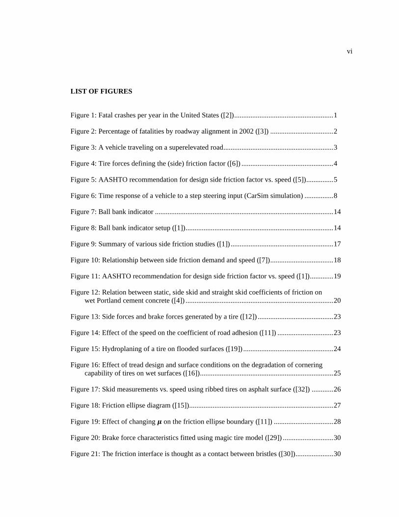
In 2002, approximately 25% of the fatalities that occurred in crashes occurred along
horizontal curves [3], as shown in Figure 2. Compared to highway tangents, the average accident
rate for horizontal curves is about three times higher [4]. Torbic et al. [3] characterized the types
of problems that occur at horizontal curves by analyzing crash data. The authors noted that the
most prevalent crash types at these locations are run-off-road (ROR) and head-on crashes.
Statistics from the Fatality Analysis Reporting System (FARS) [2] show that 76 percent of curve-
related crashes are single-vehicle crashes in which the vehicle left the roadway and struck a fixed
object or overturned, while 11 percent of curve-related fatal crashes were head-on crashes. Thus,
ROR and head-on crashes account for 87 percent of fatal crashes at horizontal curves. It is
important to determine whether the current design policy offers acceptable horizontal curve
design guidelines.
Figure 2: Percentage of fatalities by roadway alignment in 2002 ([3])
The basic physics of a vehicle traveling on a horizontal curve can be explained by a
centripetal acceleration towards the center. This acceleration is supported by the friction force
generated between the tires of the vehicle and the pavement as well as a component, of the
weight, , of the vehicle as shown in Figure 3. Superelevation or road banking is responsible for
this component of the weight of the vehicle acting parallel to the road surface and supporting the
centripetal acceleration.

3
The quantitative guidelines for the geometric curve design exist only for horizontal
curves on level roads but not for curves on downgrades. As shown later in this study, the vehicles
maneuvers on horizontal curves with downgrades are more critical than those without any grade.
This study is aimed at developing different physics-based vehicle models to determine the
acceptable road geometries for curves with downgrades. Vehicle models ranging from simple
analytical models to low-order simulation models are used and the results are verified with high-
fidelity multi-body simulations.
1.1 AASHTO Policy
American Society of State Highways and Transportation Officials (AASHTO) is the
body responsible for setting the standards and developing guidelines for highway design in the
United States. AASHTO‟s publication A Policy on Geometric Design of Highways and Streets
[5], often called the “Green Book”, gives the guidelines for horizontal curve design. A simple
model called as the point mass model, wherein a vehicle is approximated by a point mass
traveling around a curve, is the basis of these guidelines as will be shown in later chapters. The
frictional requirements of the vehicle during negotiation of a curve are represented by the side
friction factor or side friction demand. This side friction factor/demand, , is the ratio of
cornering force to normal reaction on a tire as shown in Figure 4.
Figure 3: A vehicle traveling on a superelevated road

4
Figure 4: Tire forces defining the (side) friction factor ([6])
A basic curve formula that governs vehicle operation on a curve is obtained from the
point mass model, whose derivation is shown later, is given by:
(1.1)
where is the vehicle speed in m/s, is the curve radius in m, and is the superelevation or
banking of the road expressed in meters drop per 100 meters of distance.
Using the basic side friction formula (1.1), one can find a minimum curve radius for a
given superelevation and a design speed if the limit on the side friction factor is known.
AASHTO recommends limits of the side friction factor, called the design side friction factor
( ) for each design speed as shown in Figure 5. More discussion on this follows in the
literature review of chapter 2.
Using equation (1.1) minimum curve radius for a particular design speed V is given by:
(
) (1.2)

5
where is minimum curve radius and is the maximum design side friction factor
Equation (1.2) is used in the Green Book [5] to develop quantitative guidelines for the
horizontal curves on flat roads. The basic side friction formula, (1.1) does not include the effect
of grade. AASHTO‟s policy statement [5] for horizontal curve design with downgrade reads as
follows:
On long or fairly steep grades, drivers tend to travel faster in the downgrade than
in the upgrade direction. Additionally, research has shown that the side friction demand is
greater on both downgrades (due to braking forces) and steep upgrades (due to the
tractive forces). Some adjustment in superelevation rates should be considered for grades
steeper than 5 percent. This adjustment is particularly important on facilities with high
truck volumes and on low-speed facilities with intermediate curves using high levels of
side friction demand.
In the case of a divided highway with each roadway independently superelevated,
or on a one-way ramp, such an adjustment can be readily made. In the simplest practical
form, values from Exhibits 3-25 to 3-29 can be used directly by assuming a slightly
higher design speed for the downgrade. Since vehicles tend to slow on steep upgrades,
the superelevation adjustment can be made by not reducing the design speed for the
upgrade. The appropriate variation in design speed depends on the particular conditions,
especially the rate and length of grade and the magnitude of the curve radius in
comparison to other curves on the approach highway section.
On two-lane and multilane undivided roadways, the adjustment for grade can be
made by assuming a slightly higher design speed for the downgrade and applying it to the
whole traveled way (both upgrade and downgrade sides). The added superelevation for
the upgrade can help counter the loss of available side friction due to tractive forces. On
Figure 5: AASHTO recommendation for design side friction factor vs. speed ([5])

6
long upgrades, the additional superelevation may cause negative side friction for slow
moving vehicles (such as large trucks). This effect is mitigated by the slow speed of the
vehicle, allowing time to counter steer, and the increased experience and training for
truck drivers.
There are no quantitative guidelines for adjustment in the geometry of a curve to include
the effect of downgrade. The goal of this study is to develop such design guidelines for the
possible combinations of downgrade and curvature.
1.2 Motivation
One of the main limitations of the point mass model used for horizontal curve design is
that it ignores force differences seen on different tires and axles of the same vehicle. It does not
account for the per-axle force generation capabilities of a vehicle. Nearly all vehicles have very
different tire loads on the front and rear axles caused by the center-of-gravity of a vehicle not
being located midway between the axles. For example, a typical passenger vehicle has a 60/40
weight split from front to rear. In a turn, this weight difference means that the lateral forces
required on the front axle are usually much different than the rear axle. In the case of passenger
vehicles the weight split may be 50 percent higher on the front axle. Classical vehicle dynamics
models like the bicycle model, in which the vehicle is represented as having front and rear tires
but no width, takes into account per-axle tire forces. This allows differentiation between
individual wheel friction factors which can differ from the simple point mass model [6].
Tire-pavement interaction generates friction forces that act on a vehicle during braking
and/or cornering operations and are called the friction demand. This is limited by the friction
supply, i.e. the maximum friction forces that can be generated between tire and road. When a
vehicle is braking on a curve it uses a part of the available tire-pavement friction for the braking
in longitudinal direction. As a result, less friction is available in the lateral direction for cornering.
Also, tire-pavement friction is known to decrease with speed on a wet road due to partial
hydroplaning [10]. It is not clear if these two phenomenon were explicitly considered in the

7
Green Book while developing the design side friction factors. This uncertainty is because the
Green Book [5] does not provide the friction supply values used for developing the horizontal
curve design policy. This study will make use of physics-based tire models as well as friction
measurements obtained from field experiments to determine the total available friction as a
function of speed on a wet road. These results will be used to determine whether vehicle
maneuvers on road geometries designed using current policies demand more or less friction than
the available friction supply.
Another limitation is that the point mass model is not capable of analyzing the transients
occurring before a vehicle reaches steady state. “Steady state” is the stage where all the states of a
vehicle are in equilibrium; while the behavior of the vehicle before it reaches the steady state is
called its “transient response”. Figure 6 depicts this by presenting time-response of vehicle yaw
rate to a step steering input, where one can see that before the vehicle reaches steady-state yaw
rate, it undergoes a few oscillations. The handling qualities of an automobile depend greatly upon
its transient response [7]. A transient vehicle model like the bicycle model may predict higher
friction demands compared to a steady-state model. Therefore, a horizontal curve designed for
steady-state behavior of a vehicle may prove insufficient for transient response of the vehicle.
In recent years there has been an increasing use of multi-body vehicle dynamics
simulations for highway design and safety [8, 9]. These multi-body simulations are highly
accurate and can be used to benchmark the low-order model simulation. This study uses low-
order vehicle dynamics models for their simplicity, but verifies the simulation results with the
multi-body simulations.

8
1.3 Proposed Vehicles Models
A range of models will be considered in this study for the analysis of maneuvers on
highway curves with steep grades and it is important to understand the reasons for using different
models of varying complexity for this study. These model families can be roughly classified as:
1) Modified point mass model
2) Bicycle model (Steady-state analysis)
3) Modified bicycle model (Transient analysis)
4) Multi-body simulation model
The selection of the model will require tradeoffs between simplicity, accuracy, and ease
of use. A more complex model means that a larger number of parameters are needed with higher
order differential equations. Table 1 lists the input parameters needed for each model. The grey
colored boxes indicate the input parameters considered for that particular model.
Figure 6: Time response of a vehicle to a step steering input (CarSim simulation)

9
Table 1: Model inputs for different vehicle models according to level of complexity
The most desirable model is one that is sufficiently complex to accurately describe the
behavior of interest but also the model should also be easily solved. The solution should avoid
unnecessary complexities which can slow down the simulation process and confuse the analysis
of the main effects. These competing principles require analysis-specific tradeoffs: a model useful
for a roadway study on friction limits may be wholly inappropriate for a study of vehicle rollover
on the same road surface.
The point mass model, which is a subset of the modified point mass model, is the basis of
current geometric curve design policy. The point mass model, despite its limitations, may turn out
to be sufficient to design acceptable roadway geometries. Sufficiency can be justified on the basis
of simulation results from other complex models. On the other hand, the simulation results from
the vehicle models may highlight areas of disagreement with the point mass model. The point
mass model may not be sufficient for certain road geometries and vehicle maneuvers. In that case,
more complex models may be needed to determine the acceptable road geometries.

10
1.4 Thesis Overview
The background, methodology, and results for horizontal curve design for downgrades
using low-order vehicle models are described in the following chapters. This section gives an
outline of the next chapters.
Chapter 2 presents the literature survey of highway design related studies in the past.
Tire-pavement friction studies and tire models are reviewed. The vehicle models used in literature
for the purpose of horizontal curve design are also discussed.
Chapter 3 presents the range of design variables and vehicle classes that will be used for
further analysis. The permutation levels for each road geometry parameter are stated. Chapter 3
also discusses the tire-pavement-friction model that will be used for finding friction supply
values. This model will help in determining if the friction demand is within the friction supply
limit.
Chapter 4 develops a modified analytical point mass model for three-dimensional road
geometry and also presents the static rollover models. Static rollover models will complement the
modified point mass model by adding rollover prediction capability, putting a limit on lateral
acceleration of the vehicle to ensure it does not roll over.
Chapters 5 and 6 are aimed at developing methodology for using a bicycle model for
steady-state and transient analysis of three-dimensional road geometries. The steady-state bicycle
model can predict the per-axle friction demand for a given road geometry and vehicle maneuver.
On the other hand, the transient model can predict the transients before the vehicle response
reaches the steady state.
Chapter 7 validates the simulations performed using low-order vehicle models with
CarSim simulations. Multi-body simulations were performed using high-fidelity vehicle
dynamics simulation software to validate the low-order model simulations.
Chapter 8 summarizes the results from this study and discusses the scope for future work
in highway design.

11
References
1. Mannering, F.L. et al., Principles of Highway Engineering and Traffic Analysis, John
Wiley & Sons, Inc., Third edition, 2005
2. Fatal Accident Reporting System (FARS). National Highway Traffic Safety
Administration, National Center for Statistics and Analysis. http://www-
fars.nhtsa.dot.gov/
3. Torbic, D. J. et al., Guidance for Implementation of the AASHTO Strategic Highway
Safety Plan, Volume 7: A Guide for Reducing Collisions on Horizontal Curves,
NCHRP Report 500, Volume 7, Transportation Research Board, Washington, D.C.,
2004
4. Glennon, J. C. et al., Safety and Operational Considerations for Design of Rural
Highway Curves, FHWA/RD-86/035. Federal Highway Administration, U.S.
Department of Transportation. 1985
5. American Association of State Highway and Transportation Officials, A Policy on
Geometric Design of Highways and Streets, Washington, D.C., 2004
6. MacAdam, C.C., et al., Side Friction for Superelevation on Horizontal Curves, Final
Technical Report Volume II, The University of Michigan Transportation Research
Institute, 1985
7. Bundorf R.T., A Primer on Vehicle Directional Control, Warren, Michigan: General
Motors Technical Center, 1968
8. Hamblin, B. et al., Utilization of Vehicle Dynamic Simulations as Predictors of
Highway Safety, Paper Number IMECE2007-42195, ASME IMECE, New York, NY
2007
9. Stine, J. et al., Analyzing the influence of median cross-section design on highway
safety using vehicle dynamics simulations, Accident Analysis and Prevention Volume
42, Issue 6, pp. 1769-1777, 2010

12
10. Wong, J.Y., Theory of Ground Vehicles, John Wiley and Sons, Inc. 2008
11. CarSim, Mechanical Simulation Corporation. 2006. http://www.carsim.com

Chapter 2
Literature Review
The basic side friction formula (1.1) gives an estimate of required side friction for a
vehicle maneuver on a horizontal curve. It can immediately be noted that one of the most
important factors in the horizontal curve design is , i.e. the design side friction factor from
minimum curve radius formula (1.2). It is thus critical to understand the literature supporting the
design side friction factors that are recommended by AASHTO, and the supporting studies
justifying these recommendations.
Additionally, different physics-based and semi-empirical tire models are widely used for
vehicle dynamics simulations and there is a large amount of literature available in this area. These
tire models will be reviewed since we need to use a tire-pavement friction model to develop
friction supply boundaries. Unfortunately, most of the vehicle dynamics research addresses
vehicle maneuvers on flat and dry roads/pavement, but even so, these pavement friction studies
provide data for available tire-pavement friction for wet roads.
Finally, previous efforts to use vehicle dynamics models for highway design will be
reviewed.
2.1 AASHTO Design Friction Factor
The Green Book [1] mentions that “(A) key consideration (in AASTO's policy) in
selecting maximum side friction factors for use in design is the level of centripetal or lateral
acceleration that is sufficient to cause drivers to experience a feeling of discomfort and to react
instinctively to avoid higher speeds”. It was assumed that at low speeds, drivers are more tolerant
to discomfort and hence higher values of design side friction are sought.

14
A number of studies were done in 40‟s and 50‟s on the driver behavior while driving
around the horizontal curves. These studies were focused on studying what drivers perceive as
“comfortable lateral acceleration” at different speeds. The findings from these studies became the
main factor in determining the design side friction factor ( ) in Green Book.
Barnett [2] defined the safe speed as “...the minimum speed, at which the centrifugal
force, created by the movement of the vehicle around the curve, causes the driver or passenger to
feel a side pitch outward.” In this early work, 900 road test reports were studied and side friction
factor (as calculated from the equation 1) was observed to lie in 0.10-0.20 range. Barnett assumed
a trend of the side friction factor of 0.16 for speeds of 60 mph and less, and a 0.01 decrease for
each 5 mph further increase in the speed. He also introduced an idea of the margin of safety as a
difference between the friction factor at impending skid and the friction factor when a side pitch
is first noticed.
Figure 7: Ball bank indicator
([3])
Figure 8: Ball bank indicator setup ([1])
The ball bank indicator (shown in Figure 7, setup shown in Figure 8) is typically used to
measure lateral accelerations to set the design speeds on the curves that will avoid a discomfort.

15
The ball bank indicator is a crude (by modern standards) inclinometer that measures the lateral
acceleration/side friction in degrees, on a vehicle negotiating a horizontal curve.
One of the earliest ball-bank indicator studies was done by Moyer & Berry [4] in 1940.
They investigated ball-bank indicator readings as a measure of “centrifugal force”,
superelevation, speed and curvature. They recommended the following criteria (Table 2).
Table 2: Side friction factors for various speed ranges
Speed (mph) Ball bank indicator reading
for safe speed
Design Side Friction
Factor(recommended)
14 degrees 0.21
25 and 30 12 degrees 0.18
10 degrees 0.15
Meyer (1949) recommended that a greater margin of safety should be used at higher
speeds than suggested by comfort considerations alone. Meyer recommended exponential curve
type variation for side friction vs. speed to empirically fit his data. He then used the following
relationship (2.1) to calculate corresponding ball bank angles for recommended side friction
factors.
(2.1)
( =Side friction factor, =Ball bank angle, =Body roll angle)
The ball bank angles were calculated and the body roll angles used were averages reported by
General Motors Proving Ground experiments.
During the same time period, Stonex and Noble [5] performed high speed tests on the
Pennsylvania turnpike. These tests were performed with skilled drivers and side friction values
were calculated for those tests. They suggest a lower design side friction factor than those

16
measured in the tests to ensure safety. They further recommended that the curve radii of highways
should be expanded to accommodate a design side friction factor of 0.10. At higher speeds, he
suggested the following relationship (2.2) to determine superelevation recommendations.
(2.2)
In more recent studies, Carlson [6] revisited methods to measure lateral acceleration in a
banked turn. He correlated ball-bank indicator readings with the unbalanced lateral acceleration
using regression method for speeds ranging up to 40 mph. He suggested the following
formulation (equation 4) to predict ball-bank angle indicator reading:
(2.3)
BBI= ball bank indicator reading (deg.)
ULA= unbalanced lateral acceleration or side friction factor (in ‟s)
Carlson also mentioned that the influence of body roll is negligible for passenger cars
while predicting the ball bank angle. Table 3 compares maximum side friction factors
recommended by Carlson with those from previous study by Moyer and Berry. Carlson
recommends slightly higher maximum side friction factors than Moyer & Berry based on his
studies. Again, these results appear to be based primarily on comfort.
Table 3: Comparison of side friction factors for various speed ranges
Ball bank indicator reading
for safe speed
by Moyer
& Berry
using Carlson
Model
14 degrees 0.21 0.24
12 degrees 0.18 0.21
10 degrees 0.15 0.17

17
From this past work, it should be clear that different studies have recommended different
upper limits on the design side friction factors. The Figure 9 summarizes these studies.
Figure 9: Summary of various side friction studies ([1])
A recent NCHRP study by Bonneson [7] estimated statistical models of curve speed and side
friction demand that could be used together to develop limiting values of side friction demand for
use in horizontal curve design. Bonneson made two observations: 1) Drivers appear to reduce
speed on curves and 2) they do not slow down to one common curve speed for a given radius.
Also, higher approach speed lowers side friction demand but higher speed reductions are
associated with higher side friction demand. Equation (2.4) represents the statistical model by
Bonneson calibrated using operating speed and curve geometry data that were collected at 55
sites in eight states.
(2.4)
: 85th percentile side friction demand factor, : 85th percentile approach speed (km/h), : 85th
percentile curve speed (km/h), : Calibration coefficients, : Indicator variable (=1.0 if
; 0 otherwise)

18
Based on this formula (2.4) and basic curve formula (1.1), a curve speed model was
proposed in this study. The relationship between maximum side friction demand and horizontal
curve approach speed mentioned above is shown in Figure 10. The model illustrates that side
friction demand decreases as the curve approach speed increases, while the side friction demand
increases as the speed reduction between the curve approach speed and the speed at the mid-point
of a horizontal curve ( – ) increases. The side friction demand related to no speed reduction
between the approach tangent and mid-point of a horizontal curve ( – ) was
proposed as the desirable upper limit on design side friction factors. However, a maximum
desirable speed reduction of was proposed to balance traffic flow and construction cost,
thus allowable maximum side friction demands corresponding to the – trend line
was recommended.
Figure 10: Relationship between side friction demand and speed ([7])
Based on these studies and some early pavement friction studies mentioned in the next
section, AASHTO‟s Green Book (2004) recommends use of Figure 11 to determine maximum
side friction factors for a given design speed. It is unclear that which of the studies were referred
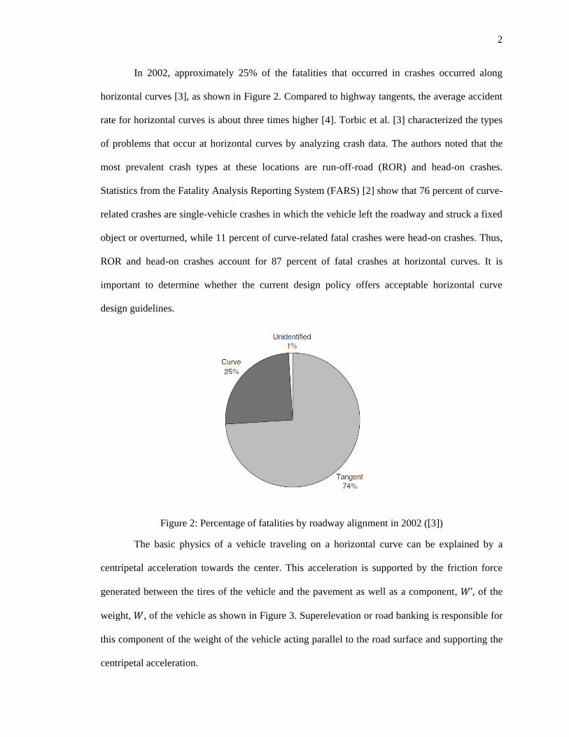
19
to for this final recommendation, but it is also clear that the AASHTO guidelines of Figure 5 form
a general fit to the previous recommendations in Figure 4. The trend of side friction factor (f) vs.
design speed (V) indicates that, at low speeds, design criteria arise from studies of comfortable
acceleration. And for speeds above 40 mph, the design side friction factor ( ) is simply
decreased at a constant rate, by a value of 0.01 for each additional 5 mph as recommended by
studies from the 1940‟s.
Figure 11: AASHTO recommendation for design side friction factor vs. speed ([1])
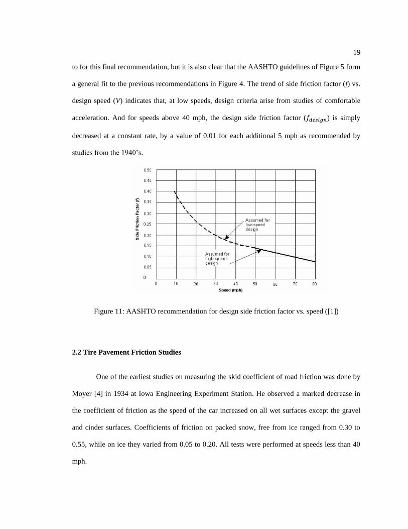
2.2 Tire Pavement Friction Studies
One of the earliest studies on measuring the skid coefficient of road friction was done by
Moyer [4] in 1934 at Iowa Engineering Experiment Station. He observed a marked decrease in
the coefficient of friction as the speed of the car increased on all wet surfaces except the gravel
and cinder surfaces. Coefficients of friction on packed snow, free from ice ranged from 0.30 to
0.55, while on ice they varied from 0.05 to 0.20. All tests were performed at speeds less than 40
mph.

20
Figure 12: Relation between static, side skid and straight skid coefficients of friction on
wet Portland cement concrete ([4])
Table 3 lists different coefficient of friction values recorded by Moyer and Figure 12
shows variation in friction levels (for different skid conditions) with respect to speed. In Table 3,
it is interesting to notice that side skid coefficients of friction reported are higher than straight
skid coefficients of friction, which is usually not the case in modern measurements of tire
behavior. The differences might be explained by Wong‟s explanation in “Theory of Ground
Vehicles,” [11] where he notes that modern passenger vehicles now use synthetic rubber which
has significantly different properties versus natural rubber, which is still sometimes used in truck
tires. The difference is that natural rubber has much better wear properties – ideal for trucks. But
the friction coefficient is lesser for the trucks compared to a passenger vehicle, assuming both had
high-grip tires of good condition [8].

21
Table 4: Coefficient of friction vs. speed ([4])
Type of Surface Type of
Skid Remarks
Coefficient of Friction
Speed in mph
5 10 15 20 25 30
P.c. concrete, 19
x 4.75 tires, no
chains
Side Dry Surface 1.01 1.01 0.97 0.95 0.92 0.89
Straight Dry Surface 0.94 0.90 0.86 0.83 0.80 0.77
Side Wet Surface 0.78 0.75 0.72 0.69 0.66 0.64
Straight Wet Surface 0.67 0.63 0.59 0.55 0.51 0.46
Ice on pavement,
no chains
Side Smooth tread 0.20 0.19 0.19 0.20 - -
Side New tread 0.19 0.19 0.22 0.19 - -
Ice on pavement,
16 x 7.00 tires, no
chains
Straight New tread 0.18 0.15 0.17 0.21 - -
Impending New tread 0.17 0.19 0.19 0.19 - -
Side New tread 0.19 0.19 0.19 0.18 - -
In latter sections, it will be seen that friction guidelines may be influenced by the required
stopping distance, and indeed it is common to see engineers incorrectly use the friction
measurements obtained from stopping distance interchangeably with the friction available for
lateral forces. Recent work examining stopping distance includes that of Olson [8] who did a
study on parameters affecting stopping distances for NCHRP 270. Based on the experimental data
and other results given in the previous studies, he proposed following equation (5) for skid
number for a given velocity (V)
(2.5)
where : Skid Number (=100 X coefficient of friction) at given speed, : Speed in mph, :
Normalized skid gradient (<0) etc.

22
Table 5 summarizes the formulae given by Olson for sliding friction & maximum rolling
(or peak) friction by passenger car tire & truck tire. The friction coefficients for the truck tires are
less than those for the passenger cars. Olson‟s study also indicates a decrease in friction with the
increasing speed.
Table 5: Olson's formula for forward friction coefficients
Passenger Car Tire Truck Tire
Sliding Friction ( )
Peak Friction ( )
Bonneson [7] uses these friction supply values given in Olson‟s study for the NCHRP
study. As explained further in this section, the tire-pavement friction depends on many factors
including road wetness, pavement properties etc. Hence, for this study, a different approach is
followed to get the friction supply values. The field measurements for specific tire-pavement
conditions are combined with the physics-based tire model to find the peak friction coefficients
rather than using empirical formulae like the ones in Table 5.
Figure 13 illustrates a typical tire curve showing the difference between peak and sliding
friction values. The peak value of braking force is usually around 1.3 times the skid
value of braking force for the dry roads, and thus the friction values in both directions
will be similarly different. In the lateral direction, in contrast, the sliding and peak tire forces are
usually about the same. Also, the lateral sliding friction usually matches the longitudinal sliding
friction, as expected since pure sliding of the tire does not differentiate the direction. However,
this situation of pure-sliding during braking is increasingly uncommon in practice due to
widespread deployment of anti-lock braking systems (ABS).

23
Figure 13: Side forces and brake forces generated by a tire ([12])
One of the most important factors affecting tire-pavement friction is the road wetness. It
has been observed that for the dry pavements there is no significant change in the tire-road
pavement friction with increasing speed, perhaps 10 to 20% at most. But there is a noticeable
decrease in friction on wet surfaces with increasing speeds. The friction is found to be decreasing
with increasing speeds as shown in Figure 14. This variation also depends on the type of road,
condition of tire treads, etc. Note that the shapes of these curves roughly match the “comfort”
curves empirically determined by civil engineers as noted in Section 2.1! It thus seems likely that
driver “comfort” may simply be a driver‟s perception of inferred friction available on wet roads.
Table 5 lists the values of peak and side coefficients of friction for different modern tires on dry
as well as wet road surfaces.
Figure 14: Effect of the speed on the coefficient of road adhesion ([11])

24
Table 6: Values of coefficient of road adhesion for truck tires on dry and wet concrete pavement
at 64 km/h ([11])
Hence, it seems appropriate to use wet road conditions for finding the friction supply
values. But challenge of wet roads is defining what the term “wet” implies in terms of surface
cover. On a wet road, at a particular speed, the hydrodynamic lift developed under the tire may
become equal to the vertical load, and tire rides completely on the fluid. This phenomenon is
referred to as the hydroplaning effect [11], shown in Figure 15.
Figure 15: Hydroplaning of a tire on flooded surfaces ([19])
At the limits of water depth, the tire-pavement friction force decreases to zero during
hydroplaning. The transition to hydroplaning (with respect to speed and water depth) causes a

25
decrease in the available friction, so that the hydroplaning effect is gradual, with increasing speed
and assuming constant water thickness on the road surface. However, if a vehicle suddenly
encounters standing water or similar near-instantaneous changes in surface water thickness, the
effect is a corresponding near instantaneous change in surface friction. For this reason, drivers
often associate hydroplaning as an “instant” effect rather than a gradual transition.
As mentioned previously, friction decreases with speed on wet pavements and this
decrease can be difficult to predict. The decrease in friction is dependent not only on the speed
and the tread conditions, but also on the water depth. As shown in the Figure 16, the available
lateral force can go to zero at 50 mph for 0.3 in. water depths. Also, for a relatively smaller
magnitude of the water depth (0.04 in.), the available side force can be significantly reduced due
to the smooth tread. However, highway agencies use 0.5 mm as the “just wet” level of water film
thickness. This can be supported by the fact that most of the modern friction measuring devices
perform measurements on surface with 0.5 mm (0.02 in.) water depth [33].
Figure 16: Effect of tread design and surface conditions on the degradation of cornering
capability of tires on wet surfaces ([16])
26
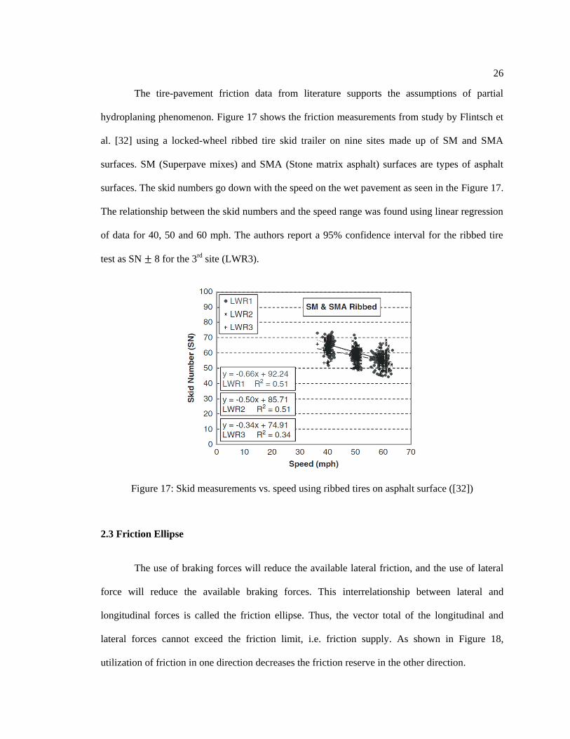
The tire-pavement friction data from literature supports the assumptions of partial
hydroplaning phenomenon. Figure 17 shows the friction measurements from study by Flintsch et
al. [32] using a locked-wheel ribbed tire skid trailer on nine sites made up of SM and SMA
surfaces. SM (Superpave mixes) and SMA (Stone matrix asphalt) surfaces are types of asphalt
surfaces. The skid numbers go down with the speed on the wet pavement as seen in the Figure 17.
The relationship between the skid numbers and the speed range was found using linear regression
of data for 40, 50 and 60 mph. The authors report a 95% confidence interval for the ribbed tire
test as SN 8 for the 3rd site (LWR3).
Figure 17: Skid measurements vs. speed using ribbed tires on asphalt surface ([32])
2.3 Friction Ellipse
The use of braking forces will reduce the available lateral friction, and the use of lateral
force will reduce the available braking forces. This interrelationship between lateral and
longitudinal forces is called the friction ellipse. Thus, the vector total of the longitudinal and
lateral forces cannot exceed the friction limit, i.e. friction supply. As shown in Figure 18,
utilization of friction in one direction decreases the friction reserve in the other direction.

27
Figure 18: Friction ellipse diagram ([15])
The friction ellipse equation represents the operating range of tire forces and is given as
[11]:
(
)
(
)
(2.6)
Since friction factor is force divided by vertical load, a modified version of the friction
ellipse equation is given as [14]:

28
(
)
(
)
(2.7)
As long as value of “ ” is less than 1, the operating point (i.e. tire forces in x and y
direction) lies inside the friction ellipse (Figure 12). The term “ ” in Equations 19 and 20, can be
referred to as the utilized amount of tire-pavement friction or the measure of friction reserve
typically used by vehicle dynamics community. One can usually infer that enough friction reserve
is available as long as . When , the friction reserve is exceeded.
It can be easily seen that the equation (2.6) represents inside of an ellipse on a
plot as shown in Figure 19. The boundary of this friction ellipse region are determined by the
(or ) and (or ). As seen previously in the section 2.2, the friction
supply goes down when a vehicles speeds up on a wet pavement. In that case the values of
and decrease, and that result in shrinking of the friction ellipse as shown in Figure 19.
Figure 19: Effect of changing on the friction ellipse boundary ([11])
To summarize the last two sections, the maximum lateral force acting on a tire or the
lateral friction supply depends on a number of factors. The main factors are summarized as:
1) The normal force on the tire (Fz), due to static weight and load transfer effects;

29
2) Longitudinal tire force (Fx), due to the friction ellipse;
3) Road surface condition (dry, wet, snow, ice etc.), due to hydroplaning and friction
reduction;
4) Vertical load acting on the tire (N);
5) Speed (mainly for wet surfaces) (V), due to hydroplaning effects;
6) Tire condition (new, worn-out); and
7) Tire composition
2.4 Tire Models
A tire model is essential for vehicle dynamics simulation and control design. There are
various tire models used is vehicle dynamics community. Tire models involve different level of
accuracy and complexity. Pacejka [12] classifies tire models as follows:
1) Empirical models: Fitting full scale tire test data by regression techniques e.g.
magic tire model
2) Similarity method based model: Using distortion, rescaling and multiplications
of one measured curve, new relationships are obtained to describe off-nominal
conditions
3) Simple physics-based model: Using simple mechanical representation,
possibly closed form solution e.g. Dugoff model, LuGre model
4) Complex physics-based model: Describing tire in great detail, computer
simulation and finite element method
Bakker et al. [29] performed a series of tire measurements and came up with a curve fit
formula. They used a special function Y(X) to fit characteristics of side force, brake force and
self-aligning torque as shown in equation (2. 8). X represents slip angle or longitudinal slip. This

30
curve fit formula is known as magic tire formula or Pacejka model and it is widely used in vehicle
dynamics simulation.
{ }
(2. 8)
Figure 20: Brake force characteristics fitted using magic tire model ([29])
De Wit et al. [30] developed a physics based friction model for control systems with
friction. Their model, called as LuGre model, takes into account Coulomb friction, viscous
friction and Stribeck effect. The interface between two surfaces was represented by bristles as
shown in Figure 21.
Figure 21: The friction interface is thought as a contact between bristles ([30])

31
The deflection of bristles was represented by a variable z. The bristle deflection dynamics
was given by:
| |
(2.9)
where |
⁄ |
And the longitudinal force per unit normal force was given by:
⁄ ⏟
⏟
⏟
(2.10)
where : relative velocity between 2 surfaces, : normalized coulomb friction, : normalized
static friction, : Stribeck velocity, =0.5 used for tire modeling, are model constants
The steady-state net force per unit normal force obtained by integrating along the tire contact
patch for a distributed model and assuming constant normal load distribution over tire patch is
given by:
⁄ ( [
(
)] ) (2.11)
where |
|
, L=contact patch length (0.2 m),
The equation (2.11) is a modified version of original steady-state solution and is given in
[31] where is pre-multiplied by a factor . accounts for the variations in pavement
characteristics, road wetness and other factors that are difficult to model directly. Figure 22 shows
plots of coefficient of friction in longitudinal direction for different velocities and values
obtained using modified equation of LuGre model. In section 2.2, we saw that tire-pavement
friction reduces on wet road. In this study, the parameter is be used to represent the partial
hydroplaning phenomenon. The parameters required to calculate friction coefficient in equation
(2.11) are found by calibration with field measurement data. Figure 23 shows an example of
using experimental data to calibrate LuGre model.

32
Figure 22: Static view of distributed LuGre model under different values for v ( =1) and (v=20
m/s) over full range of longitudinal slip ([31])
Figure 23: Calibrating LuGre model with the experimental data ([31])

33
2.5 Vehicle Dynamic Models
2.5.1 Two-axle Vehicle Models
Although the point-mass model serves as the basis for horizontal curve design, over the
past few decades some researchers have proposed two-axle models, (i.e., the “bicycle model”) for
horizontal curve design (Figure 24). The models in these studies represent modifications to the
classical bicycle model used in vehicle stability analysis, a model that is derived and discussed in
detail in subsequent sections. The modifications include factors such as aerodynamic forces, body
roll, grade, braking/acceleration, friction ellipse, etc.
Figure 24: Bicycle model
The advantage of the bicycle model versus the point mass model is that it examines not
only force balance, but also moment balance keeping the vehicle from “spinning out” on a
roadway. Further, it is useful to examine whether individual axles will exhibit skidding prior to
the entire vehicle exhibiting skidding. For example, Psarianos et al. [14] studied the influence of
vehicle parameters on horizontal curve design. Although their focus was primarily on passenger
cars, they compared their results with the corresponding values accepted by AASHTO (1990)
design policy as well as RAS-L-95 (German Highway) design policy. They used a friction ellipse
equation (Equation (2.7)) to check if the friction reserve (n) is exceeded. Additionally, they
developed a two-axle vehicle model (steady-state) for curves on grades and calculated the friction
factors. They considered the vehicle maneuvers at speeds exceeding design speed by 10-20 km/h

34
(6-12 mph). It is not clear if they considered different superelevation rates for their analysis on
vertical grades. Their analysis indicates that the friction reserve might be exceeded for a
passenger car traveling 20 km/h (12 mph) higher than the design speed of 80 km/h (on a
minimum curve radius obtained from basic point mass model analysis) for downgrades more than
5%. They pointed out that these maneuvers will be more critical for trucks since they have lower
maximum side friction factors. Table 7 lists the utilized amount of friction for a passenger car for
maneuvers 10 and 20 km/h (6 and 12 mph) above a design speed of 80 km/h (50 mph).
Table 7: Utilized amount of total available friction supply for mini passenger car moving on a
curve (with downgrade) with Rmin for Vd= 80 km/h ([14])
Downgrade (%)
Vd+ 10 km/h Vd+ 20 km/h
0 0.66 0.89
1 0.68 0.91
2 0.70 0.93
3 0.73 0.95
4 0.76 0.98
5 0.79 1.01
6 0.82 1.04
7 0.86 1.08
8 0.90 1.11
9 0.94 1.15
Kontaratos et al. ([17]) also developed an analytical two-axle vehicle model to determine
the minimum horizontal curve radius as a function of vertical grade. In their bicycle-like model,
the authors‟ added the effects of the grade and superelevation, front wheel vs. rear wheel drive,
air resistance, etc. Superelevation was assumed to be 7 percent for all cases analyzed. This
analysis considered only the driving mode of vehicle on grades, and not any braking situations
that would occur in downgrades. They suggest from this analysis a modified basic curve formula
for minimum curve radius:

35
⁄
(2.12)
The factor “ ” depends on air resistance, height of CG, mass of vehicle, grade angle etc. “ ” has
different expressions for front wheel drive and rear wheel drive case. is the maximum side
friction factor in the lateral (y) or side direction. The maximum longitudinal friction factor (in
direction of braking) was assumed to be maximum (peak) value of coefficient of friction and the
maximum lateral friction (in the side direction) was assumed to be the sliding value of the
coefficient of friction.
To illustrate how the available friction in the lateral (side) direction is reduced with an
increase in the grade for the same design speed, Kontaratos et al. used the friction ellipse equation
to check if the friction reserve is exceeded. Their results are shown in Table 8, and suggest that
the safety margins for the friction factor are lower on steeper grades. They note that a
comprehensive analysis is needed with a complete driver-vehicle-road system model for better
analysis of road features.
Table 8: Demand values of fx for various speeds and grades, and remaining friction reserve to be
used in lateral direction fy (values from AASHTO-1990) ([17])
Downgrade
(%)
V85=50 mph V85=60 mph V85=70 mph
fx fy fx fy fx fy
0 0.09 0.29 0.12 0.27 0.16 0.25
3 0.17 0.27 0.20 0.25 0.24 0.21
6 0.25 0.23 0.28 0.19 0.14 0.14
One of the key studies in horizontal curve design (without grade) using vehicle models
was done by MacAdam et al. [22] at UMTRI. They used steady-state and transient bicycle model
as well as tractor-trailer model for horizontal curve design and verified their simulations with the
field experiments. They concluded that point mass model based curve design can be sufficient for
nominal conditions. They noted that wheel to wheel friction can significantly vary on a turn. They

36
mention that on a low friction pavement, tractor-semitrailer requires approximately 10% higher
friction levels than those suggested by the point mass model.
Finally, Bonneson (2000) developed a two-axle vehicle model in NCHRP Report 439
(Figure 25). This is one of the most detailed (analytical) vehicle dynamics model used so far in
the literature on horizontal curve design. This model was based on the static analysis of forces
acting on a turning vehicle. Only mild braking (ax=0.85 m/s2) was considered (representative of
the speed reduction upon an entry to the curve). The decrease in margin of safety (for the side
friction factor) for trucks and passenger cars was reported on grades. Bonneson considered only
two-axle vehicles for the analysis (passenger car, single unit-truck etc.). He developed the slide
(skid) failure and roll failure models separately to check if vehicle maneuvers are safe at given
conditions.
Figure 25: Bicycle model used by Bonneson ([7])
Note that none of the studies mentioned above, except MacAdam [22], consider a multi-
axle vehicle model and thus omit all tractor trailers. Further, very few of these models consider a
tire model inclusive of the friction ellipse and representative combined braking/turning situations.
Many of them do not address load transfer, transient instabilities, and many steady-state
instabilities as well.

37
2.5.2 Bicycle Model Instabilities
In the vehicle dynamics literature, one finds many papers relevant to vehicle stability
while turning on a horizontal curve, although none of these are clearly used at present in
AASHTO policy. One class of bicycle model instabilities is often obtained under what is known
as “steady-state” conditions, e.g. constant steering inputs, constant road radii, etc. The results of
the steady-state analysis show strong similarity to the NCHRP Report 439 model [7]. These,
governing equations predict that stability will depend on velocity-squared terms. With
assumptions similar to those used in the point-mass model, constant radius curves, known vehicle
and road properties, etc., the bicycle model can be used to calculate the forces and moments on
each axle of the vehicle. These forces and moments can be used to obtain conditions for stability
or instability in terms of vehicle-specific understeer or oversteer factors called “understeer
gradients” [13]. For passenger vehicles, this determines the “critical speed” above which an
oversteer vehicle will become unstable.
For multi-axis vehicles, these stability derivations can be used to predict whether (and at
which speeds) the vehicle will exhibit a “trailer jackknife” type of instability. A front wheel lock-
up of the tractor trailer results in the loss of the directional control and the vehicle moves in a
straight line. A rear wheel lock-up results in the loss of the directional stability resulting in an
accidental folding of the articulated vehicle, called jackknifing (shown in Figure 26). This is most
likely to occur when the low normal force or excessive braking force is experienced by the rear
tractor wheels. The maximum lateral force that can be generated in a cornering by a tire depends
on the vertical load acting on the tire. A wheel locking of the trailer would result in the loss of the
directional stability of the trailer and results in the swinging of trailer outside the curve (as shown
in Figure 27).

38
Figure 26: Tractor-trailer jackknifing
Figure 27: Trailer wheel lock-up
If a driver applies a steady steering input (for example, during transition from a straight
road to a horizontal curve) and maintains it, the vehicle will enter a turn of constant radius after a
transition period. The behavior of the vehicle in this transition time period is called its “transient
response characteristics”. Bundorf [18] pointed out that such a behavior is quite important and
the handling qualities of an automobile depend greatly upon its transient response. Fortunately,
the bicycle model can predict curve onset transient behavior and other transient effects commonly
observed in driving, for example maneuvers such as a lane change where the radius of horizontal
curve is changing. This is important because road accidents are often caused by precipitating
events and rapid steering inputs that occur in addition to the steady-state forces and driver inputs
needed to negotiate a long sweeping turn. The transients associated with such maneuvers are
widely studied in the vehicle dynamics community and discussed in vehicle dynamics papers
([20], [21]) and textbooks ([15], [11], [13] and [12]). These transients are generally ignored in
roadway design guidelines based on point-mass models or even in steady-state bicycle models.
Although the classical bicycle model is very useful to address instabilities described in
the previous section, it has the following limitations [15]:
It does not include lateral load transfer effects;

39
It does not include longitudinal load transfer;
It assumes linear tire ranges (cornering less than 0.4g), and thus is not valid near friction
limits;
It assumes that there are no rolling or pitching motions;
It assumes quasi-constant forward velocity;
There are no suspension compliances; and
There is no aerodynamics (although this effect is readily added).
In terms of relevancy to this project, the primary critique of the bicycle model
assumptions above is the one ignoring a vehicle‟s roll dynamics and tire vertical loading. While a
vehicle is negotiating a turn, there can be a lateral load transfer due to lateral acceleration, torque
generated by engine, road geometry, or combination of these. Hence, the vertical forces acting on
inner and outer tires are not the same. The cornering (lateral) force produced by the tires usually
does not change linearly with the normal load (depending upon tire type and operating point on
the curve) as shown in Figure 28. Hence, the net lateral force provided by the left and right tires
might actually be less compared to the case where there is no lateral load transfer. Hence, higher
slip angles may be required to get the same net lateral force.
Figure 28: Cornering force vs. normal load ([11])

40
Figure 29 shows the cornering stiffness vs. normal load for different types of tires. Note
that passenger car tires might be more sensitive to lateral load transfer since they typically operate
near the peak of the curve, while truck tires operate in relatively linear range of the curve.
Figure 29: Cornering stiffness vs. normal load for different tires ([11])
To take the lateral load transfer into account, a roll angle model is needed in combination
with the bicycle model. In vehicle dynamics studies, low-order rollover models are considered to
take into account the effect of roll. A recent study by Hamblin et al. (2006) looked at various
vehicle models that include roll dynamics effects (e.g., a 3 DOF model with sprung mass). It was
observed that relatively simpler (low-order) models show good agreement with field experiments.
Figure 30 from a key study by UMTRI [22] illustrates importance of lateral load transfer effect on
the variation of side to side friction factor. Thus, determining whether roll stability and load
transfer are important considerations in the geometric design of high-speed curved roadways is an
important consideration.

41
Figure 30: Side to side friction factor variation ([22])
There is also a possibility of a longitudinal load transfer due to acceleration/braking or
road geometry (grades). This load transfer might be of concern since the cornering stiffness is
dependent on the normal load (Figure 29). During braking scenarios, if the lateral force on rear
tire(s) is saturated first (compared to that on front tire), the vehicle might oversteer. This case is
called a „Limit Oversteer‟ condition. A limit oversteer vehicle loses directional stability and
might be susceptible to a crash. If the front tires are saturated first, the vehicle will not lose
directional stability, but it might lose directional control (limit understeer). Vehicles contain brake
proportioning valves to prevent this type of instability; however, the geometric design of the
roadway may tax one axle of a vehicle to an extent that limit oversteer effects are observed.

42
2.5.3 Multi-body Models
A multi-body model representation of a vehicle requires use of numerical solvers to
calculate solutions of differential equations derived from laws of physics and kinematics of the
vehicle. A number of commercial vehicle simulation packages are available that allow one to
perform multi-body vehicle dynamics simulations; e.g. CarSim and TruckSim [23], HVOSM
[24], ADAMS [25] etc. A detailed history of vehicle simulation packages can be found in [26].
Some of the past highway design studies have used multi-body simulation packages. A
study by Glennon et al. [27] used HVOSM to conduct investigation on the effects of cross-slope
braking on highway curves. A study at UMTRI [22] used the Phase 4 simulation package of
UMTRI for horizontal curve design study. Bonneson [7] used HVOSM for a small part of his
study. A recent study by Stine et al. [28] used CarSim [23] to analyze influence of median cross
section design on the highway median safety using simulation.
In these simulations, models of the tire dynamics, tire vertical motion, the suspension
vertical motion, and body vertical/roll/pitch motion are included in addition to the typical
lateral/longitudinal/yaw motion included in a bicycle model. These multi-body simulations are
quite complex and can take several orders of magnitude more computations to simulate versus a
bicycle model formulation. However, they are also exceptionally accurate. Their errors are so
small, usually a few percent error for a well-calibrated model, that they are widely used in the
automotive industry as a replacement for field testing for chassis stability analysis.

43
References
1. American Association of State Highway and Transportation Officials, A Policy on
Geometric Design of Highways and Streets, Washington, D.C., 2004
2. Barnett, J., Safe Side Friction Factors and Superelevation Design, Highway Research
Board 16, Washington, DC, 1936
3. Ball Bank Indicator by Rieker manufactures,
http://www.riekerinc.com/ballbankindicators.htm
4. Moyer, R. A., and Berry, D. S., Marking highway curves with safe speed indicators,
HRB Proc. 20, page 399–428, 1940
5. Stonex, K.A., and Noble., C.A., Curve Design and Tests on the Pennsylvania
Turnpike, Highway Research Board 20, Washington DC, pp. 429-451, 1940
6. Carlson P.J., Correlation of Ball Bank Indicator Readings and Lateral Acceleration,
Ph.D. Thesis, The Pennsylvania State University, 1995
7. Bonneson, J. A., NCHRP Report 439: Superelevation Distribution Methods and
Transition Designs, Transportation Research Board, Washington, D.C., 2000
8. Olson, P. L. et al., Parameters Affecting Stopping Sight Distance, NCHRP Report
270, Transportation Research Board, National Research Council, 1984
9. Ervin, R.D., Mobile Measurement of Truck Tire Traction, in Proc. Symposium on
Commercial Vehicle Braking and Handling, Highway Safety Research Institute,
University of Michigan, Ann Arbor, 1975
10. Fancher, P.S. et al., A Fact Book of the Mechanical Properties of the Components for
Single-Unit and Articulated Heavy Trucks, Report No. DOT HS 807 125, National
Highway Traffic Safety Administration, U.S. Department of Transportation, 1986
11. Wong, J.Y., Theory of Ground Vehicles, John Wiley and Sons, Inc. 2008

44
12. Pacejka, H.B., Tire and Vehicle Dynamics, SAE International, 2006
13. Gillespie, T., Fundamentals of Vehicle Dynamics. SAE International Press, 1992
14. Psarianos, B. et al. Influence of Vehicle parameters on Horizontal Curve Design of
Rural Highways, Transportation Research Circular E-C003, p. 22:1-10,
Transportation Research Board, 1998
15. Milliken, W.F., and Milliken, D.L., Race Car Vehicle Dynamics, SAE International,
August 1995
16. Horne, W.B. et al., Pneumatic Tire Hydroplaning and Some Effects on Vehicle
Performance, Society of Automotive Engineers, Paper 650145, 1965
17. Kontaratos, M. et al., Minimum Horizontal Curve Radius as a Function of Grade
incurred by Vehicle Motion in the Driving Mode, Transportation Research Record
1445, TRB, National Research Council, Washington D.C., pp.86-93, 1994
18. Bundorf, R.T., A Primer on Vehicle Directional Control, Warren, Michigan: General
Motors Technical Center, 1968
19. Clark, S. K., Ed., Mechanics of Pneumatic Tires, Monograph 122, Washington, DC:
National Bureau of Standards, 1971
20. Dugoff, Howard, On the Influence of Aerodynamic Forces and Moments on the
Lateral Stability of Articulated Highway Vehicles Detroit, pg. 215-245, 1968
21. Ito, K. et al "Stability Analysis of Automatic Lateral Motion Controlled Vehicle with
Four Wheel Steering System" Proceedings of the 1990 American Control
Conference, San Diego, CA, pg. 801--808, May, 1990
22. MacAdam, C.C., et al., Side Friction for Superelevation on Horizontal Curves, Final
Technical Report Volume II, The University of Michigan Transportation Research
Institute, 1985
23. CarSim, Mechanical Simulation Corporation. 2006. http://www.carsim.com

45
24. HVOSM, McHenry Software. 2006. http://www.mchenrysoftware.com
25. ADAMS, MSC Software. 2006. http://www.mscsoftware.com
26. Bridget, H., Vehicle Rollover Prediction from Low Order Dynamic Models or
Varying Terrain Encountered During Median Traversal, M.S. Thesis, Mechanical
Engineering, The Pennsylvania State University, August 2007
27. Glennon, J.C. et al., HVOSM Studies of Cross-Slope Breaks on Highway Curves,
Final Report, FHWA, 1981
28. Stine, J.S., et al., Analyzing the Influence of Median Cross-Section Design on
Highway Median Safety Using Vehicle Dynamics Simulations, University Park: The
Pennsylvania State University 2009
29. Bakker, E. et al., A New Tyre Model with Applications in Vehicle Dynamics Studies,
4th Autotechnologies Conference, Monte Carlo 1989, SAE Paper 890087, P. 83-95
30. De Wit, C.C. et al., A New Model for Control of Systems with Friction, IEEE
transactions on Automatic Control, Vol. 40, no. 3, 1995
31. De Wit, C.C. et al, Dynamic Friction Models for Road/Tire Longitudinal Interaction,
Vehicle System Dynamics, Vol. 39, No. 3, P. 189-226, 2003
32. Flintsch, G.W. et al., Speed Adjustment Factors for Locked-Wheel Skid Trailer
Measurements, Transportation Research Record 2155, P. 117-13, Washington D.C.,
2010
33. Hall, J.W. et al., Guide for Pavement Friction, NCHRP project 1-43, Transportation
Research Board of the National Academics, Washington D.C., 2009

Chapter 3
Design Space and Tire-Pavement Friction Model
The geometric design of horizontal curves includes a number of elements like grade,
curve radius, superelevation etc., which affect the performance of a vehicle on a turn. The vehicle
performance methodology used in this study to evaluate the geometric curve design is presented.
Also, an explanation about the permutations of geometric design elements that are considered for
the subsequent analyses is given. Apart from the geometric design elements, the vehicle
performance also depends on the design of a vehicle and its maneuver on the curve. The vehicle
classes and the vehicle maneuvers that are used later in this thesis are given. This study uses a
friction demand versus friction supply analysis while evaluating curve design. Hence, a tire-
pavement friction model used to obtain the supply friction values is also described in the latter
part of the chapter.
3.1 Methodology
Current highway design policy [1] uses a simple point mass model along with design side
friction factors ( ) for the geometric design of horizontal curves. Figure 31 shows the point
mass model being used to find the minimum curve radius based on the design speed of the curve,
the superelevation and the design side friction factor. The formula for minimum curve radius is
given by equation (1.2). The design side friction factor is a function of the road design speed [1].
Hence, the minimum radius of a curve simply depends on the design speed and the road
superelevation. The design speed is thus used as an overall control in the design of highway
curves.

47
Figure 31: Methodology diagram
A curve may be referred to as a “sharp curve” if the curve has the minimum radius for a
given design speed. It is important to check if the sharp curves offer enough friction supply for a
vehicle cruising at a design speed, especially when the curves are combined with downgrades.
Vehicle dynamics models discussed in section 1.3 are used to check if sharp curves offer enough
friction supply. As seen in the friction comparison block of Figure 31, friction demand ( )
for a vehicle is calculated for various downgrades and deceleration levels on a sharp curve. The
friction demand for a particular scenario is compared with the friction supply value to find if the
road design is acceptable. The friction supply values are obtained using the field measurement
and a tire-pavement friction model as described later in section 3.4.
If the friction demand exceeds the friction supply for a curve (shown in the output of
friction block in Figure 31) modifications are to be made to the road geometry in order to provide
sufficient friction supply. One possible approach for ensuring adequate friction supply is to

48
modify the design friction factor ( ) for that particular downgrade and design speed
combinations.
The next few chapters are dedicated to developing the vehicle dynamics models which
are used to find the friction demand on sharp curves.
3.2 Design Variables
This study considers a range of superelevations, horizontal curve radii, design speeds,
grades, and deceleration levels. For a simple turn, the road geometry of a curve can be
represented by a superelevation rate, a horizontal curve radius and a grade. The basic vehicle
maneuver can be described in terms of a design speed and a constant (or zero) deceleration. These
parameters are referred to as “design variables” and affect the required friction for a vehicle to
travel around a sharp curve. The permutations of design variables considered for the simulations
are discussed in this section.
According to [1], design speeds of roadways vary from 10 to 80 mph in the intervals of 5
mph. The 10 to 40 mph range is considered to be the low speed range and the 40 to 80 mph range
is considered to be the high speed range. Only the high speed range is considered for this study in
order to focus on the curve design for highways.
Superelevation is an important geometric curve design factor since higher superelevation
rates allow for shaper curves (using equation (1.2)), and AASHTO recommends a maximum
superelevation value of 12%. Superelevation is generally not used for low-speed urban streets [1].
For high speed road designs, maximum superelevation rates of 4, 6, 8, 10 and 12 percent are used.
Note that superelevation rates of 4% or higher are considered because of the superelevation
distribution method used. This method (called as “Method 3” in Green book) is generally used for
high speeds and emphasizes the use of maximum superelevation rate for high speed curves

49
(Figure 32). Superelevation rates of 4% to 12% incremented at 1% interval are considered for this
study.
AASHTO recommends a maximum grade value of 9%. The Green book also mentions
that some adjustment in the current policy might be needed for grades greater than 5%. This
research investigates the impact of all the ranges of grades starting from 0%, i.e. flat roads, rather
than assuming the current superelevation criteria are sufficient for grades of 5% and below. To
allow the same tolerance levels for grade as those for superelevation, an interval of 1% is chosen
for the grades as well.
Only generic road designs are considered for this research, i.e. it is assumed that road
geometry variables (e, R, G) are constant for a turn. Cases such as a spiral road with varying
curve radius are not considered. The superelevation transition from a crown slope on the tangent
section to a superelevation on the curve section is also neglected. It is assumed that the lateral
slope of the road, i.e. superelevation remains constant from the end of the tangent section
throughout the curve.
Table 9 summarizes the discussion above and lists the values of road geometry variables.
Only sharp curves i.e. minimum radius curves are considered for analysis since they represent the
highest friction demands.
Figure 32: Superelevation distribution with inverse of curve radius ([1])

50
Table 9: Design space described using road geometry variables
Variable Input Parameter Range
v 40 to 60 mph (5 mph interval)
e 4% to 12% (1% interval)
G 0% to -9% (1% interval)
As mentioned in section 1.4, the use of braking increases the friction demanded by a
vehicle on a turn. It is thus important to highlight the deceleration levels that are considered in
this study. A vehicle cruising at a constant design speed, i.e. zero deceleration, is a basic scenario
for travel on a curve with downgrade. A recent study by Bonneson [2] mentions that drivers adopt
typical deceleration levels of around 0.85 m/s2 to reduce their speed while entering a curve. Both
of these cases are considered for this thesis.
During braking situations where vehicles must stop for an obstacle ahead of the vehicle,
AASHTO mentions that approximately 90% of the drivers decelerate at the rates greater than 3.4
m/s2. It is assumed by AASHTO that the friction available on most wet pavements and the
capabilities of most vehicle braking systems can provide braking friction that exceeds 3.4 m/s2
deceleration rate. The 3.4 m/s2 deceleration is used to find the “stopping sight distance”, i.e. the
minimum length of a road required for a vehicle to stop before reaching a stationary
object/obstacle in the path. The braking distance, , on a flat road is given by [1]:
(3.1)
where is the design speed in m/s and is the stopping sight deceleration, 3.4 m/s2.
The stopping sight distance for downgrades take into account the effect of downgrade. The
braking distance, , for downgrades is given by [1]:
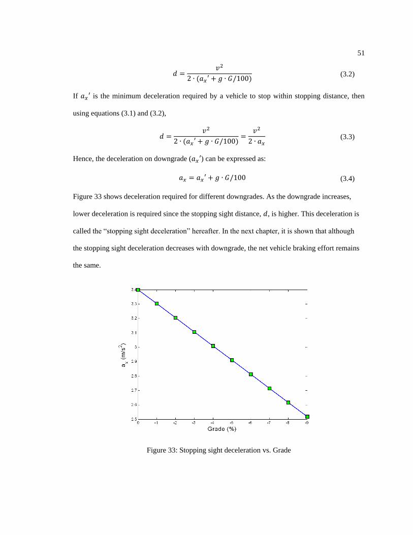
51
(3.2)
If is the minimum deceleration required by a vehicle to stop within stopping distance, then
using equations (3.1) and (3.2),
(3.3)
Hence, the deceleration on downgrade ( ) can be expressed as:
(3.4)
Figure 33 shows deceleration required for different downgrades. As the downgrade increases,
lower deceleration is required since the stopping sight distance, , is higher. This deceleration is
called the “stopping sight deceleration” hereafter. In the next chapter, it is shown that although
the stopping sight deceleration decreases with downgrade, the net vehicle braking effort remains
the same.
Figure 33: Stopping sight deceleration vs. Grade

52
In addition to these decelerations, an emergency deceleration situation is considered.
AASHTO mentions that most drivers decelerate at a rate greater than 4.5 m/s2 when confronted
with the need to stop for an unexpected object in the roadway. Hence, the 4.5 m/s2 is considered
as an emergency braking deceleration for this study. Table 10 summarizes the deceleration levels
used in this study.
Table 10: Deceleration vales for each maneuver type
Maneuver Type Deceleration Value (m/s2)
Cruising at constant speed 0
Speed reduction on curve entry 0.85
Stopping sight deceleration 3.4 +
Emergency braking 4.5
3.3 Vehicle Family
To simulate vehicle models other than the point mass model, one must know per axle or
per tire forces. The simulations may also depend on transient (curve-entry stability) and non-
planar motion (wheel lift) that is vehicle-specific. The family of the vehicles will be important
for subsequent analysis because each vehicle class can have different friction demands depending
upon the vehicle-specific parameters.
To “define” a vehicle, each of the models needs a number of vehicle input parameters,
such as the weight distributions between axles, the CG height, suspension properties, etc. A set of
vehicle parameters representative of general vehicle classes are needed for these analyses. For
many vehicles, representative parameters are defined in the literature as well as in commonly
used vehicle dynamics software, for example in CarSim. The input parameters needed for each
vehicle type are:

53
1) Inertia Properties: Mass (m), Z-axis mass moment of inertia about CG of total vehicle
(Izz)
2) Dimensions: Wheelbase (L), CG height (hCG), Distances from CG of sprung/unsprung
mass to front/rear axle along x-axis, Track Width (t), Roll center height (hroll)
Again, the intent is to define representative vehicles, yet ones that represents the most
deserving of attention for specific design of downgrade turn geometries. It is proposed to use the
following vehicle classes from the passenger car fleet: 1) E-class Sedan 2) E-class SUV. Vehicle
specific parameters are listed in Appendix B for each of the vehicle class.
3.4 Tire-Pavement Friction Model
It is important to define the longitudinal peak friction supply values since those truly
represent the maximum longitudinal friction supply when ABS is on. Tire-pavement friction
measurements on wet roads are usually available only for full skidding. The LuGre tire model is
one of the few physics-based tire models that consider effects of the road wetness. For this study,
the tire-pavement friction measurements from the literature [32] are combined with the modified
LuGre model [5] to find the longitudinal peak friction supply values ( ).
The tire-pavement friction measurements from a study by Flintsch et al. [32] are used as
the inputs to the LuGre tire model. Most of the friction measurements available in literature are
recorded for speeds below 60 mph. The friction measurements from this study were chosen since
skidding tests were performed on modern tire-pavement combination. Modern tire measurements
are performed on road with 0.5 mm water depth [33] which is described as the “just wet”
condition, by highway agencies (FHWA, AASHTO).
Based on the Flintsch‟s study [32], the skid coefficients for the 40 to 60 mph range can be
estimated by equation (3.5). These coefficients were obtained on asphalt surfaces using locked

54
wheel ribbed tire testing machine. The authors also report the 95% confidence interval for skid
measurements is . The lower limit of friction measurements is chosen for a conservative
design.
(3.5)
The relative velocity ( ) between tire surface and pavement can be assumed to be same
as vehicle speed ( ) when a tire skids on the road, i.e. in the case of locked wheel braking test.
The rotational velocity of the tire ( ) is zero in this case. The LuGre model review can be used to
express the longitudinal friction coefficient, , for this scenario. For the skidding case, the
longitudinal friction factor can be written (by referring to equation (2.11)) as follows
(3.6)
where | ⁄ |
The value of factor used can be found by solving equation (3.6).
(3.7)
The steady state longitudinal force per unit normal force can be obtained by substituting the value
of from equation (3.7) into equation (2.11),
⁄ (
[
(
)] )
(3.8)
Using equation (3.8), the longitudinal friction coefficient can then be obtained as a function of
longitudinal slip to find the peak friction factor(s) as shown in Figure 34. Note that the values of
LuGre parameters used here are found by calibration using field experiments in the study [5].
Once the longitudinal friction coefficient is known for all the slip conditions, the maximum/peak
longitudinal friction coefficient can be found.

55
The LuGre model combined with the friction measurements gives the peak longitudinal
friction values, i.e. longitudinal friction supply ( ). The lateral friction supply limit ( )
can be assumed to be same as the skid coefficients obtained in the field measurement.
Figure 34: LuGre model calibrated using friction measurements
The friction supply values obtained from this tire-pavement friction model are used for
the analysis of friction demand versus friction supply. A friction ellipse like the one shown in
Figure 35 can be generated using the friction supply values obtained from the tire-pavement
friction model. An operating point ( ) represents the friction demand. If the operating point is
within the friction ellipse, , then the corresponding road design would be
acceptable.

56
Figure 35: Friction ellipse and operating point

57
References
1. American Association of State Highway and Transportation Officials, A Policy on
Geometric Design of Highways and Streets, Washington, D.C., 2004
2. Bonneson, J. A. NCHRP Report 439: Superelevation Distribution Methods and
Transition Designs. Transportation Research Board, Washington, D.C., 2000
3. Flintsch, G.W. et al., Speed Adjustment Factors for Locked-Wheel Skid Trailer
Measurements, Transportation Research Record 2155, P. 117-13, Washington D.C.,
2010
4. Hall, J.W. et al., Guide for Pavement Friction, NCHRP project 1-43, Transportation
Research Board of the National Academics, Washington D.C., 2009
5. De Wit, C.C. et al, Dynamic Friction Models for Road/Tire Longitudinal Interaction,
Vehicle System Dynamics, Vol. 39, No. 3, P. 189-226, 2003
6. De Wit, C.C. et al., A New Model for Control of Systems with Friction, IEEE
transactions on Automatic Control, Vol. 40, no. 3, 1995
Chapter 4
Modified Point Mass Model and Static Rollover Model
The simplest vehicle model that can be considered for the horizontal curve design
problem and the basis of the AASHTO horizontal curve design recommendations is a point mass
model of a vehicle on a superelevated road of a constant curve radius. The point mass model
derivation is shown in this chapter, with a modification to include the effect of downgrades. By
treating an automobile as a point mass on three-dimensional road geometry and applying
Newton‟s laws of motion, such a model can be used for the friction demand versus friction supply
analysis. To complement the modified point mass model, a static rollover model is presented
towards the end of this chapter.
4.1 Coordinate System
An SAE axis system (Figure 36) will be used for developing equations of motion for all
the vehicle models in this study. This axis system ( ) is fixed to the vehicle (body) with -axis
pointing downwards. The origin is located at vehicle CG (center of gravity). Inertia values
relative to coordinate frame are assumed to be constant [1].
Since this is a steady-state analysis, it can be assumed that the global origin corresponds
to the local origin (vehicle CG) as shown in Figure 37. In the global coordinate system ( ),
plane corresponds to a flat terrain and -axis is pointed in a direction opposite to gravity. The
local (SAE) axes are at an angle to the global axes since the vehicle is going down on a curve
with superelevation and downgrade .

59
Figure 36: SAE coordinate system ([1])
Figure 38 shows the side view and rear view of a point mass traveling on a three
dimensional road. The superelevation, , is defined as rise (or drop) in meters per 100 meters of a
horizontal distance [3]. It can be clearly seen from the rear view of the vehicle point mass that the
superelevation, , is given by:
(4.1)
Figure 37: Vehicle position and orientation in the global coordinate system

60
The grade ( ) is the slope of a road along the direction of travel expressed in a manner similar to
the superelevation definition. For a downgrade, the numerical value of is negative. The side
view in Figure 38 shows a vehicle point mass traveling on a downgrade. The value of grade is
given by:
(4.2)
4.2 Equation of Motion
By Newton‟s second law we know that the equation of motion for a body in an inertial
frame is given by:
(4.3)
where =Force vector acting on the point mass, m= Mass of the vehicle point mass, = Velocity
of the point mass
Since the vehicle is traveling around a curve of constant radius , the body-fixed frame is
rotating with a constant angular velocity
in the local coordinate frame [1]. The derivative
of vector referred to a rotating body frame having angular velocity is given by following
identity [2]:
Figure 38: Side view and rear view of a point mass traveling on a 3D road

61
(4.4)
where the subscripts and refer to inertial and body fixed frames of reference respectively.
Using equations (4.3) and (4.4), we get:
(4.5)
For using equation (4.5), we need to find the acceleration in the body-fixed frame and the velocity
and forces in the SAE/local axis system. As shown in Figure 39, the velocity of the point mass is
given by and the acceleration is given by
. Hence, equation (4.5) can be
rewritten as
(4.6)
A small angle approximation is used while calculating forces in the subsequent analysis.
The superelevation angle ( ) and grade angle ( ) are assumed small enough such that:
Figure 39: Vehicle velocity and acceleration
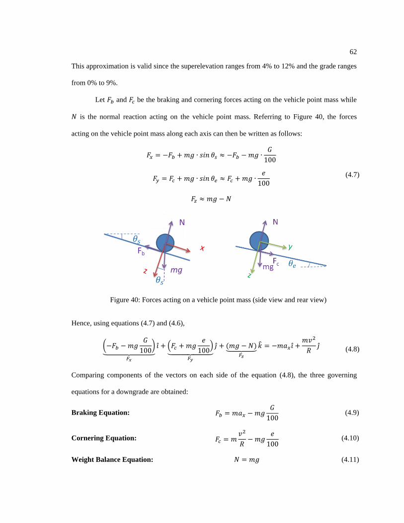
62
This approximation is valid since the superelevation ranges from 4% to 12% and the grade ranges
from 0% to 9%.
Let and be the braking and cornering forces acting on the vehicle point mass while
is the normal reaction acting on the vehicle point mass. Referring to Figure 40, the forces
acting on the vehicle point mass along each axis can then be written as follows:
(4.7)
Hence, using equations (4.7) and (4.6),
(
)
⏟
(
)
⏟
⏟
(4.8)
Comparing components of the vectors on each side of the equation (4.8), the three governing
equations for a downgrade are obtained:
Braking Equation:
(4.9)
Cornering Equation:
(4.10)
Weight Balance Equation: (4.11)
Figure 40: Forces acting on a vehicle point mass (side view and rear view)

63
The braking and cornering forces are provided by the tire-pavement friction. Highway
engineers typically use a ratio of friction force to normal reaction called as “friction factor”, to
indicate the friction demand. For this study, the friction factors are defined as follows:
Longitudinal Friction Factor
Side Friction Factor
Substituting expression for forces from braking equation (4.9) and cornering equation
(4.10), the friction factors demanded by a vehicle traversing a steady downgrade turn can be
given as follows:
(4.12)
The side friction factor ( ) is the friction factor used in the basic curve formula (1.1).
Since this study restricts itself only to sharp curve geometries, i.e. minimum radii curves, the side
friction factor can rewritten as:
(4.13)
Comparing equation (4.13) with equation (1.2), , i.e. the side friction demand is
independent of the superelevation on the sharp turns for the modified point mass analysis.
4.3 Friction Curves
The friction factors and together represent the friction demand of a vehicle point
mass. The friction supply values are available from the tire-pavement-friction model developed in
the previous chapter. In order to check if the friction demand is less than friction supply, equation
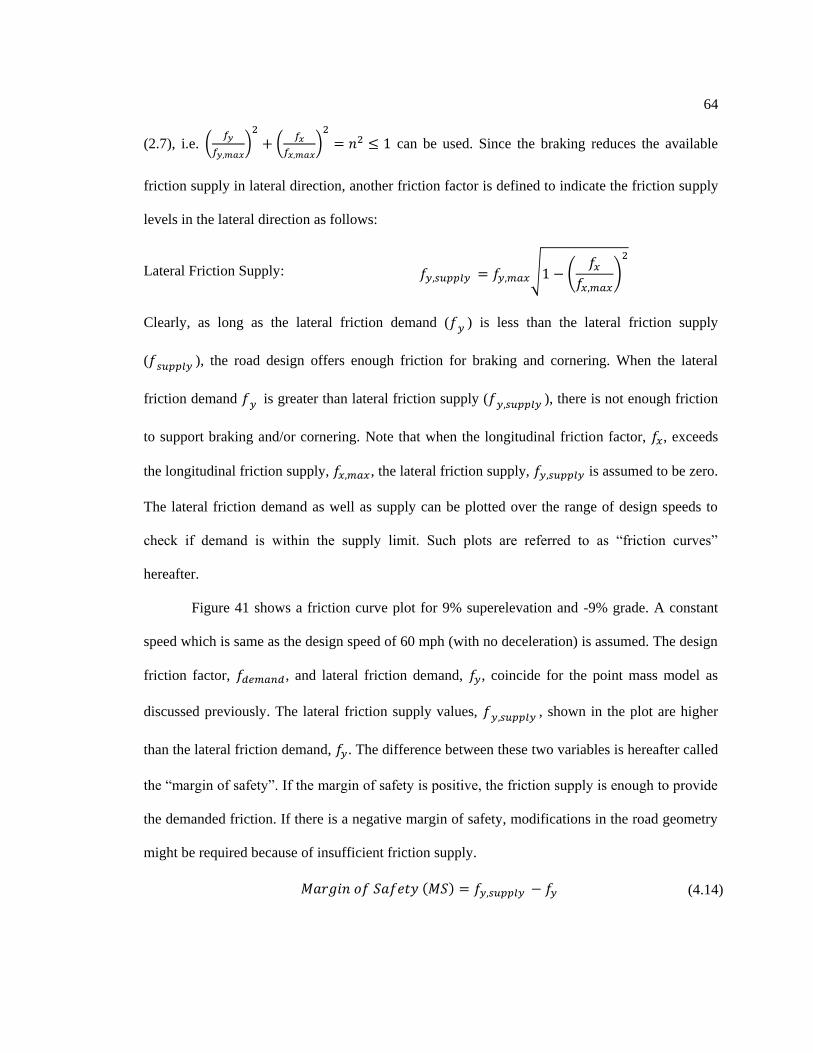
64
(2.7), i.e. (
)
(
)
can be used. Since the braking reduces the available
friction supply in lateral direction, another friction factor is defined to indicate the friction supply
levels in the lateral direction as follows:
Lateral Friction Supply: √ (
)
Clearly, as long as the lateral friction demand ( ) is less than the lateral friction supply
( ), the road design offers enough friction for braking and cornering. When the lateral
friction demand is greater than lateral friction supply ( ), there is not enough friction
to support braking and/or cornering. Note that when the longitudinal friction factor, , exceeds
the longitudinal friction supply, , the lateral friction supply, is assumed to be zero.
The lateral friction demand as well as supply can be plotted over the range of design speeds to
check if demand is within the supply limit. Such plots are referred to as “friction curves”
hereafter.
Figure 41 shows a friction curve plot for 9% superelevation and -9% grade. A constant
speed which is same as the design speed of 60 mph (with no deceleration) is assumed. The design
friction factor, , and lateral friction demand, , coincide for the point mass model as
discussed previously. The lateral friction supply values, , shown in the plot are higher
than the lateral friction demand, . The difference between these two variables is hereafter called
the “margin of safety”. If the margin of safety is positive, the friction supply is enough to provide
the demanded friction. If there is a negative margin of safety, modifications in the road geometry
might be required because of insufficient friction supply.
(4.14)

65
Figure 42 shows the margin of safety plot for the case shown in Figure 41. It can be seen that
margin of safety goes down as speed increases since the lateral friction supply decreases at a
faster rate than the lateral friction demand.
Figure 41: Friction curves for =-9% at 60 mph using modified point mass model (ax= 0 m/s2)
Figure 42: Margin of safety for =-9% at 60 mph using modified point mass model (ax = 0 m/s2)

66
Figure 43 shows a margin of safety plot for in the case of 0.85 m/s2 deceleration case.
The margin of safety goes down as the downgrade increases since the longitudinal friction
demand (braking) increases.
Figure 43: Margin of safety vs. speed on all downgrades (ax= 0.85 m/s2)
Figure 44 shows a margin of safety plot for the stopping sight deceleration case. This plot
is valid for all the superelevation rates as explained in the section 4.2. Also, the braking force in
the case of stopping sight deceleration can be obtained by combining equation (3.4) and braking
equation (4.9) as:
(
)
(4.15)
where =3.4 m/s2
Hence, the braking force for stopping sight deceleration case is independent of the grade
as well. The margin of safety in stopping sight deceleration case is least compared to other two
deceleration cases. Hence, it can be inferred that the stopping sight deceleration case is the

67
deciding factor among the three deceleration cases mentioned so far. Since the margins of safety
are all positive, it can be concluded that current horizontal curve design meets the stopping sight
distance requirements for 40 to 60 mph speed range based on the modified point mass model
analysis.
Figure 44: Margin of safety for stopping sight deceleration case (60 mph)
Figure 45 shows the margin of safety plots for “emergency braking case”. The margin of
safety goes negative for downgrades more than 6% at 60 mph. For a severe downgrade (9%), the
margin of safety goes negative even for a 50 mph speed. A negative margin of safety implies that
vehicle will skid in case of the deceleration required for the severe braking.

68
Figure 45: Margin of safety for emergency braking (ax= 4.5 m/s2)
4.4 Static Rollover Model
The point mass model developed above considers only the skid instabilities of a vehicle.
In precipitating events, a vehicle might skid or rollover depending upon the tire-pavement friction
supply and the rollover propensity of the vehicle. To complement the point mass model, a static
rollover model is developed to predict the occurrence of wheel-lift events. This model assumes
that a wheel-lift event is equivalent to a rollover event. The static rollover uses a steady-state
analysis to find the rollover threshold of a vehicle. The rollover threshold can be used as an upper
limit on the lateral acceleration experienced by a vehicle going on a turn. The static rollover
analysis considers a suspended vehicle model, meaning it considers the effects of sprung mass
roll. Although the suspension deflections are considered, the tire deflections are neglected. The
inertia of the unsprung mass is assumed negligible compared to the sprung mass. This model only
considers the lateral load transfer [13].

69
To derive the rollover model, the geometry of a wheel-lift condition is first considered.
Figure 46 shows the rear view of the suspended vehicle model for a vehicle taking a right hand
turn. Figure 46 shows the forces acting on the suspended vehicle model. Due to the lateral load
transfer the normal load on the outside wheel, , increases. This can be associated with the
sprung mass rolling with a lateral shift in the center of gravity (CG) towards the outside of the
turn. In fact, the sprung mass CG rotates about a point called the roll-center whose position
depends on the suspension geometry.
Figure 46: Rear view of a suspended vehicle model for static rollover prediction
Different parameters used for the static rollover model are listed in the Table 11.

70
Table 11: List of symbols for static rollover model
Symbol Meaning
Height of sprung mass CG
Height of roll center
Tread width
Roll angle
Normal load on inner tires
Normal load on outer tires
Lateral force on inner tires
Lateral force on outer tires
This model associates the rollover event with the normal load on the inside wheels going
to zero ( ). Hence, it can be assumed that just before rollover. Balancing the
moments about outer tire contact point,
∑ (
) (
) (4.16)
Substituting
into (4.16) and using the small angle approximation yields,
(
) (
)
(4.17)
For steady-state analysis, the roll angle can be written as the roll rate, in rad/ , multiplied
by the lateral acceleration in ‟s.
. Hence, equation (4.17) can be rewritten as

71
(
)
(4.18)
Equation (4.18) gives the rollover threshold for a vehicle. It can be easily observed that
the superelevation, , increases the rollover threshold of a vehicle, so a vehicle would be less
susceptible to rollover on a banked road. From equation (4.18), it can be seen that the lowest
rollover threshold (worst case) corresponds to the lowest superelevation of 4%. The rollover
threshold is calculated for both the Sedan and SUV vehicle class (Table 12) for a 4%
superelevation rate, the worst case. The choice of these two particular vehicle classes was made
because they have one of lowest rollover thresholds in the Sedan and SUV vehicle fleet. The
vehicle specific parameters are listed in Appendix B.
Table 12: Rollover threshold for passenger car vehicles on 4% superelevated road
Vehicle Class Rollover threshold in ’s
E-class Sedan 1.35
E-class SUV 1.13
The rollover threshold represents the lateral acceleration in ‟s that is required for a
rollover event to occur. Therefore, it is evident that if the lateral friction supply is less than the
rollover threshold value, a skidding event will occur before rollover. The friction supply values
for 40 to 60 mph are all below 0.7. For these vehicles skidding event is likely to occur first as the
lateral acceleration increases, especially when a superelevation greater than or equal to 4% is
being considered for high-speed horizontal curve design. Although this is true for passenger cars,
heavy trucks can have rollover thresholds as low as 0.35 [6]. This thesis considers only
passenger cars in the analysis and therefore, focuses on the skid events on horizontal curves rather
than rollovers.

72
References
1. Milliken, W.F. and Milliken D.L., Race Car Vehicle Dynamics, SAE International,
August 1995
2. Nelson R., Flight Stability and Automatic Control, McGraw Hill, 1998
3. Mannering F. L. et al, Principles of Highway Engineering and Traffic Analysis, John
Willey & Sons Inc., 2005
4. American Association of State Highway and Transportation Officials, A Policy on
Geometric Design of Highways and Streets, Washington, D.C., 2004
5. Gillespie, T., Fundamentals of Vehicle Dynamics. SAE International Press, 1992
6. Harwood, D.W. et al., Review of Truck Characteristics as Factors in Roadway
Design, NCHRP Report 505, Transportation Research Board, Washington, D.C.,
2003
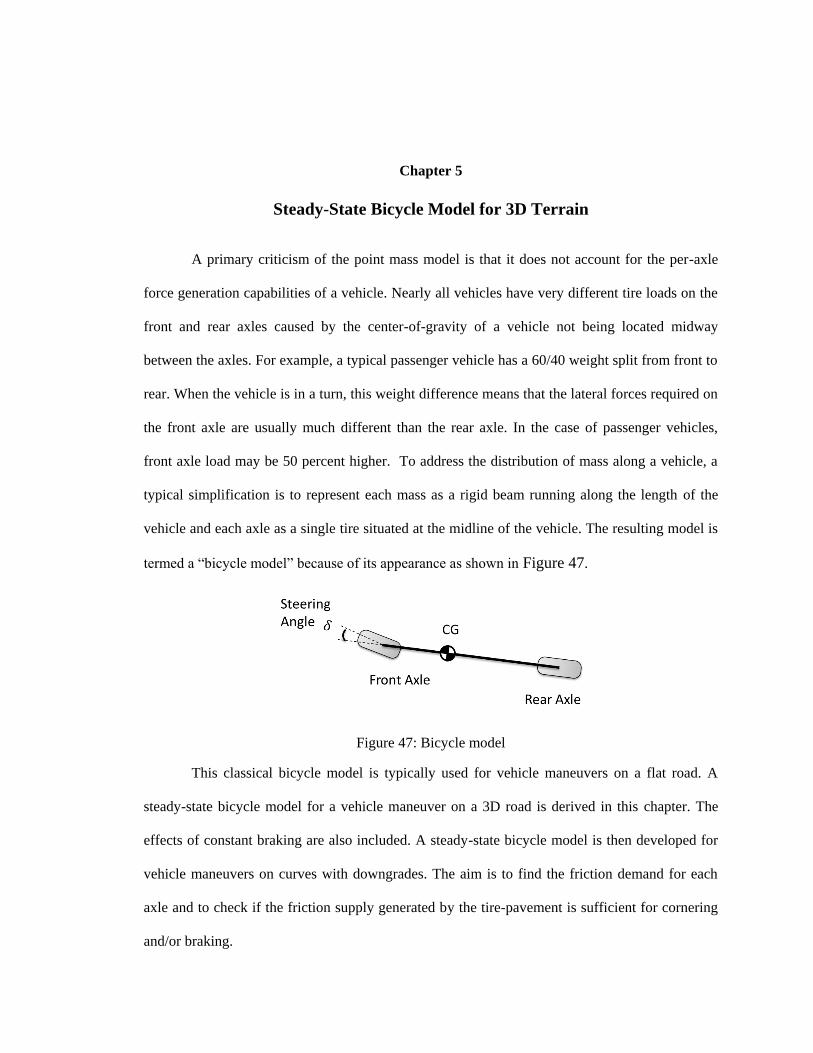
Chapter 5
Steady-State Bicycle Model for 3D Terrain
A primary criticism of the point mass model is that it does not account for the per-axle
force generation capabilities of a vehicle. Nearly all vehicles have very different tire loads on the
front and rear axles caused by the center-of-gravity of a vehicle not being located midway
between the axles. For example, a typical passenger vehicle has a 60/40 weight split from front to
rear. When the vehicle is in a turn, this weight difference means that the lateral forces required on
the front axle are usually much different than the rear axle. In the case of passenger vehicles,
front axle load may be 50 percent higher. To address the distribution of mass along a vehicle, a
typical simplification is to represent each mass as a rigid beam running along the length of the
vehicle and each axle as a single tire situated at the midline of the vehicle. The resulting model is
termed a “bicycle model” because of its appearance as shown in Figure 47.
Figure 47: Bicycle model
This classical bicycle model is typically used for vehicle maneuvers on a flat road. A
steady-state bicycle model for a vehicle maneuver on a 3D road is derived in this chapter. The
effects of constant braking are also included. A steady-state bicycle model is then developed for
vehicle maneuvers on curves with downgrades. The aim is to find the friction demand for each
axle and to check if the friction supply generated by the tire-pavement is sufficient for cornering
and/or braking.

74
5.1 Coordinate Transformations
The derivations for the bicycle model are performed in SAE (local) coordinate system.
For steady-state as well as transient bicycle models, it is useful to have coordinate
transformations defined between the local and global frames. The equations of motion can be
easily derived in a local coordinate frame, but the position and orientation of the vehicle is
realized in the global (earth fixed) coordinate frame. In this section, a rotation matrix is developed
to allow transformations from one frame to another.
To begin the description of transformations, let be a vector quantity. The components
of the vector along each axis of a Cartesian coordinate axis system depend on the orientation of
the coordinate system. Let the components of along the , and axes of the global
coordinate system be and . Similarly, let the components of along the , and axes
of the SAE body-fixed coordinate system be and . The orientation of a local frame with
respect to a global frame can be described using three Euler angles. The order in which the Euler
angles are applied is important. The following order of rotations is generally used to orient the
global frame, to the SAE local frame, .
1) Rotate frame about -axis through the yaw angle to the frame
2) Rotate frame about -axis through the pitch angle to the frame
3) Rotate frame about -axis through the roll angle to the frame
Then the transformation from local to global frame is given by [2]:
[
]
[
]
⏟
[
]
(5.1)
where etc.

75
The value of each Euler angle needs to be determined to find the rotation matrix . An
important property of the rotation matrix is that its inverse is same as its transpose [2]. Hence,
we can easily transform vectors in global frame to a local frame by pre-multiplication with .
Since this is steady-state bicycle model, it will be assumed that global and local origins coincide
at time =0. Grade and superelevation contribute to pitch angle and roll angle, respectively.
Figure 48 shows a top view of a car going around a right-hand turn. The velocity vector is along
the global -axis direction but the body-fixed -axis in the vehicle frame is at an angle with the
global -axis. This is because of the fact that the vehicle has a lateral component of velocity, ,
in addition to the longitudinal component, . The angle between the longitudinal velocity
component ( -axis) and the velocity vector is called the sideslip angle and denoted by .
Figure 48: Top view of a car going on a turn
The rotation sequence for the coordinate transformation is:
1) Yaw angle, =
2) Pitch angle, =
3) Roll angle, =

76
Using the small angle approximation, expression (5.1) can be simplified as:
[
]
[
⁄
⁄
]
⏟
[
]
(5.2)
5.2 Model Terminology
A number of vehicle specific parameters and motion variables are used in the derivation
of the equation of motion. Table 13 lists these parameters and variables.
Table 13: List of symbols for the steady-state bicycle model
Symbol Meaning
Roll rate
Pitch rate
Yaw rate
Rotational velocity
Mass of vehicle
Velocity of the vehicle
Longitudinal velocity
Lateral velocity
Deceleration along -axis
, Braking force (front and rear axle)
, Cornering force (front and rear axle)
, Normal load (front and rear axle)
Vehicle weight ( )
, CG to front and rear axle distance
Wheelbase
CG height

77
Application pressure
, Brake pressure (front and rear axle)
, Brake gain (front and rear axle)
Tire rolling radius
, Longitudinal friction factor (front and rear axle)
, Lateral friction factor (front and rear axle)
, Lateral friction supply (front and rear axle)
5.3 Equation of Motion
The equation of motion in a rotating frame as shown in section 4.2 is given by
(5.3)
A number of assumptions are being made for the steady-state bicycle model. The salient
assumptions are listed below.
Bicycle model assumptions:
1) No lateral load transfer, i.e. the vehicle compressed to a single-track (bicycle model)
2) Roll and pitch dynamics are ignored i.e. , , ,
3) is a plane of symmetry, i.e. and also
4)
5) Rolling resistance and aerodynamics are ignored
6) No chassis or suspension compliance effects
7) Pitch angle, , and roll angle, , in the rotation matrix, , are constant throughout a
vehicle maneuver
Steady-state assumptions:
1) and the deceleration, is constant
78
2)
3) and hence,
4) with ‖ ‖ and ‖ ‖
5) In the body frame,
6) A small angle approximation can be used for the grade angle, , and the
superelevation angle,
For a vehicle traveling on a curve, the local frame is a rotating frame which is a non-
Newtonian frame. For the steady-state analysis the rotational velocity can be assumed constant,
. To write the equation of motion for the steady-state bicycle model in the
form of equation (5.3), it is necessary to find velocity and acceleration vectors in the body frame
and write down the force vector in the inertial body coordinate system. To write the force vector
in the body frame, coordinate transformations will be used. Note that this derivation will be
useful later when doing transient analysis as well.
The velocity of the bicycle model in the body frame is given by
(5.4)
Assuming that the deceleration, , acts along the -axis, the acceleration vector in the body
frame is
(5.5)
The rotational velocity of the body frame is
. This analysis finds the
forces acting on the vehicle only at the beginning of braking, because the velocity of the vehicle
changes as the driver brakes. This will change the lateral forces as well as the rotational velocity
of the frame.
Combining equations (5.3) and (5.5),

79
( )
(5.6)
Referring to Figure 49, the forces acting on the vehicle in the body coordinate frame are
given as follows:
Normal Reactions:
Cornering Forces:
Braking Forces:
Weight: [
]
Combining the expressions for forces, the force vector acting on the vehicle body is given
by
(
)
⏟
(
)
⏟
⏟
(5.7)
Using equations (5.6) and (5.7), and approximating the velocity magnitude as ‖ ‖
and ‖ ‖ , the following equations are obtained:
Figure 49: Forces acting on a vehicle traveling on a curve with downgrade

80
Braking Equation:
(5.8)
Cornering Equation:
(5.9)
Weight Balance Equation: (5.10)
Note that these equations are similar to the equations (4.9), (4.10) and (4.11) obtained from the
modified point mass model. The only difference is that the steady-state bicycle model gives per-
axle forces whereas the modified point mass model gives net forces.
Since this study focuses on the sharp curves which have minimum curve radii, the
cornering equation (5.9) can be rewritten as
Combining the equation above with equation (1.2),
The design side friction factor, , depends on the design speed. Therefore, the only road
design variable affecting cornering forces is the design speed. This makes the lateral friction
demand independent of the superelevation for the steady-state analysis. The longitudinal friction
demand depends on the grade and deceleration levels as shown in braking equation (5.8).
Individual forces are obtained by the moment balance about the -axis and -axis. For the
moment balance equations, the accelerations are used as pseudo forces. Referring to Figure 50, a
moment balance about the -axis direction (at front and rear tire contact point) yields,
⁄ (
)
⁄
⁄ (
)
⁄
(5.11)

81
Figure 50: Moment Balance about -axis for rear axle
The moment-balance about the -axis gives the ratio of front and rear axle cornering
forces, shown in Figure 51.
(
⁄ )
(
⁄ )
(5.12)
Figure 51: Moment-balance about -axis
The friction factor expressions for each axle would be:
Side Friction Factors
Longitudinal Friction Factors
Using these definitions and equations (5.11) and (5.12), the side friction factors per axle are:

82
(
⁄ )
⁄ (
)
⁄
(
⁄ )
⁄ (
)
⁄
(5.13)
A model for brake proportioning is necessary for finding the longitudinal friction factors which is
discussed in the next section.
5.4 Brake Proportioning Model
The basic functions of a brake system are to slow down the speed of the vehicle, to
maintain its speed during downhill operation, and to hold the vehicle stationary after it has come
to a complete stop [4]. Passenger cars typically use hydraulic brakes which transfer braking
pressure from the controlling unit to the actual brake mechanism. Balancing the brake outputs on
the front and rear axles is achieved by “proportioning” the brake pressure appropriately for the
brakes installed on a vehicle [13]. As shown in the Figure 52, the braking torque is the product of
brake pressure and brake gain for each axle. The brake force can be obtained by dividing the
brake torque by tire rolling radius, .
(5.14)

83
Figure 52: Brake proportioning flowchart
It is well known that lock-up of the rear wheels should be avoided since this may result in
an oversteer vehicle. Hence, the brake outputs are balanced by “brake proportioning”,
appropriately adjusting the braking pressures at the front and rear axles. The brake pressure
output for the rear axle is reduced to 30% after a certain application pressure, .
for
(5.15) and for
The values of the parameters involved in this brake proportioning model are listed for the Sedan
and SUV vehicle classes in Table 14.
Table 14: Brake proportioning parameters for passenger cars
Vehicle class (N-m/MPa) (N-m/MPa) ’ (MPa) (m)
E-class Sedan 800 600 2.5 0.364
E-class SUV 800 600 2 0.385
The net braking force, required for a decelerating vehicle is given by the braking
equation (5.8) as:

84
The braking force distribution for the front versus rear axle depends on whether the application
pressure, , is greater or less than the quantity . The braking force, , when is
( )
The braking force distribution per axle can be found by considering two cases: I) and
II)
Case I)
In this case the braking forces per axle are simply:
and
.
And hence,
and
.
Case II)
In this case the braking forces per axle are given by
and
. The
values of and are different and can be found by obtaining value of the application brake
pressure, . The net braking force for this case is given by:
( )
Combining equation above with (5.15),
( )
( )
(5.16)

85
Once is known, the per-axle braking forces can be found by using equation (5.15). Using the
per-axle braking forces, the longitudinal friction factors can be found using their basic definitions,
.
The utilization of friction in the longitudinal direction reduces the friction supply in the
lateral direction and vice versa. The lateral friction supply factors are defined per axle as follows:
Front Axle: √ (
)
(5.17)
Rear Axle: √ (
)
Note that when the longitudinal friction factor exceeds the longitudinal friction supply, ,
the lateral friction supply is assumed to be zero.
5.5 Friction Curves
For steady-state bicycle model, the friction demand friction supply analysis is performed
for each individual axle. For example, if the lateral friction supply for the rear axle, , is
less than the lateral friction demand, , then the rear axle is likely to skid. This is the advantage
of using the bicycle model over the point mass model. For convenience, the difference between
lateral friction supply per axle and lateral friction per axle is defined as the “margin of safety”.
The margins of safety per-axle can be defined as:
Front Axle: ( )
(5.18) Rear Axle:

86
If lateral friction demand, , exceeds the lateral friction supply, , the margin of safety
will be less than zero. In other words, a positive margin of safety indicates acceptable road
design.
Figure 53 shows a comparison of the per-axle friction demand for a steady-state E-class
Sedan bicycle model with a point mass model for all grades and superelevation rates. The
longitudinal weight shift due to deceleration results in different per-axle friction demand. In case
of E-class SUV, this effect is more pronounced (shown in Figure 54) due to higher CG height, .
Also, like modified point-mass model, steady-state bicycle model results are independent of the
grade when stopping sight deceleration is considered.
Figure 53: Friction factors per-axle for steady-state bicycle model (E-class Sedan) compared with
the point mass model (stopping sight deceleration case)

87
Figure 54: Friction factors per-axle for steady-state bicycle model (E-class SUV) compared with
the point mass model (stopping sight deceleration case)
Figure 55 shows margins of safety for each axle of an E-class SUV compared with the
point mass model. The margin of safety for rear axle of E-class SUV goes as low as 0.12 at 60
mph but it is still positive. The brake proportioning model shows that the brake application
pressure, , is less than . This is alarming since the rear axle margin of safety is very low at
60 mph speed. This results occur because the normal load on the rear axle, , is less than the
usual which causes the lateral friction factor,
to go up and the margin of safety to go
down.
Figure 56 shows per-axle margins of safety for E-class SUV in an emergency braking
case. It can be seen that rear axle has a negative margin of safety at all the speeds on all the
grades. This implies that either the rear axle will skid for such a high deceleration or the vehicle
will not be able to achieve such a high deceleration. As the margins of safety for emergency
braking are negative even for the steady-state bicycle model analysis, the next chapter focuses on
the stopping sight deceleration case.

88
Figure 55: Margins of safety per-axle for steady-state bicycle model (E-class SUV) compared
with the point mass model (stopping sight deceleration case)
Figure 56: Margins of safety per-axle for steady-state bicycle model (E-class SUV) for
emergency braking (ax= 4.5 m/s2)
89
References
1. Milliken, W.F. and Milliken D.L., Race Car Vehicle Dynamics, SAE International
(August 1995)
2. Nelson, R.C., Flight Stability and Automatic Control, 2nd edition, McGraw Hill, 1998
3. Gillespie, T., Fundamentals of Vehicle Dynamics. SAE International Press, 1992
4. Limpert, R., Brake Design and Safety, 2nd edition, SAE, 1999
5. CarSim, Mechanical Simulation Corporation, 2006 http://www.carsim.com

Chapter 6
Modified Transient Bicycle Model for 3D Terrain
When a vehicle enters a curve from a straight road, it may slow down and/or abruptly
change its steering input. Hence it is important to consider the transient effects of constant
braking effects and abrupt steering changes. The basis of transient analysis for this study is
determining whether the driver‟s change in braking or steering inputs to the vehicle might
introduce temporarily oscillations in the vehicle motion (transient behavior) that could affect the
friction demand of each axle.
The goal of this chapter is to develop a bicycle model suitable for transient maneuver
analysis on 3D road geometry. A classical bicycle model, shown in Figure 47, is a two degree-
of-freedom model with yaw rate and lateral velocity as the motion variables. Input variables like
steering input, , and braking pressure input are under driver‟s control.
Figure 57: Bicycle model
The derivation of modified transient bicycle model involves the use of coordinate
transformations, equations of motion and a linear tire model. In the end, a vehicle maneuver is
described and the results are presented using friction curves.

6.1 Coordinate Transformations
Similar to the derivation of steady-state bicycle model, SAE coordinates are used to
derive the transient bicycle model. The coordinate transformation matrix, , is used to transform
vectors from one coordinate frame to another coordinate frame. Apart from yaw angle, the Euler
angles for transient bicycle model derivation are same as the Euler angles from the steady-state
model derivation. The Euler angles for coordinate transformation from the local coordinate frame
to global coordinate frame are:
1) Yaw angle = ∫
2) Pitch angle =
3) Roll angle =
The yaw angle, , for the transient bicycle model is different because the vehicle‟s
orientation changes in a global frame of reference as it travels around a curve, as shown in Figure
58. The yaw angle, , is summation of the vehicle‟s yaw angle (integration of yaw rate) and
sideslip angle in order to compensate for the change in orientation.
A velocity vector in local frame ( ) can be transformed to global frame
( ) using:
[
]
[
]
⏟
[
]
(6.1)
where etc. and = ∫ . The global position of the vehicle‟s center
of gravity at any time can be obtained by integrating the velocity, .

92
[ ]
∫ [
]
(6.2)
Figure 58: Change of vehicle orientation as it travels around a curve
6.2 Equation of Motion
Several of assumptions are used in the derivation of the transient bicycle model for
simplicity [1]. Most of the assumptions are similar to the steady-state bicycle model assumptions.
The additional assumptions are listed below.
1)
2) Grade ( ) and superelevation ( ) angles are constant throughout the curve
3) Linear tire range
4) Steer angle ( ) is small, i.e. the longitudinal and lateral tire forces in tire‟s axis
system are almost same as longitudinal and lateral forces in vehicle‟s body-fixed axis
system
5) Front wheel steering

93
6) Braking forces per-axle are obtained from the steady-state results
The equation of motion for a bicycle model in a rotating frame as shown in section 4.2 is
given by:
(6.3)
Velocity of the bicycle model in the body frame is given by:
(6.4)
The acceleration vector in the body frame is given by:
(6.5)
Substituting (6.3) and (6.4) into equation (6.5),
(6.6)
From steady-state model derivation in section 5.2,
(
)
⏟
(
)
⏟
⏟
(6.7)
Comparing equations (6.6) and (6.7):
Longitudinal Dynamics Equation:
(6.8)
Lateral Dynamics Equation: ( )
(6.9)
Weight Balance Equation: g (6.10)
For this study, a steady-state value of net braking force, , is used. The brake
proportioning model described in section 5.4 is used to find the per-axle braking forces, and
.

94
(6.11)
The values of normal loads acting on the front ( ) and the rear axle ( ) are found as shown in
section 5.2.
⁄ (
)
⁄
⁄ (
)
⁄
(6.12)
The yaw dynamics equation is found by balancing the moments acting along z-axis on
the bicycle model as shown in Figure 59.
Yaw Dynamics Equation: (6.13)
Figure 59: Moments and forces acting on the bicycle model
The bicycle model dynamics are represented by the equations (6.9), and (6.13) which are listed
below.
Lateral Dynamics Equation: ( )
(6.9)
Yaw Dynamics Equation:
(6.13)

95
6.3 Extension using Linear Tire Model
The tire will experience lateral slip as it rolls under cornering conditions in which the tire
must develop a lateral force, , [4]. The angle measured from the direction of heading (x‟-axis)
to direction of travel (wheel‟s velocity vector) is defined as the slip angle ( ) of the tire as shown
in Figure 60. The steer angle, δ, is the angle measured from the vehicle‟s direction of heading (x-
axis) to wheel‟s direction of heading (x‟-axis).
Figure 60: Linear Tire Model
The cornering force for a tire under a given normal load increases linearly with the slip
angle for small slip angles (5 degrees or less) [4]. The proportionality constant for the cornering
force to is called the “cornering stiffness”, . The linear tire model is used to find cornering
forces in the lateral dynamics equation (6.9). The cornering forces per axle are given by:
(6.14)
where and , are cornering stiffness for front and rear axle respectively.
The cornering stiffness strongly depends on normal load and is assumed to be linear as a
first approximation [4]. The “cornering coefficient” ( ) is defined as the ratio of cornering
stiffness to normal load ( ).

96
(6.15)
Figure 61 shows cornering stiffness at four different loads and a linear curve-fit using the least-
square method. The cornering stiffness values were obtained from [5]. The slope of the linear
curve-fit can be assumed to be the cornering coefficient ( ).
Figure 61: Cornering stiffness vs. normal load
The cornering coefficient, , is used to find cornering stiffness values per axle.
(6.16)
As seen in equation (6.14) cornering stiffness and slip angles are required to find the
cornering forces. The slip angle of the tire can be found using geometry as described in [6, 7].
(
) (
)
(
) (
)
(6.17)
Using small angle approximation, equation (6.17) is rewritten as:

97
(6.18)
Substituting (6.16) and (6.18) into (6.9),
( ) (
) (
)
(6.19)
6.4 Vehicle Maneuver
A vehicle already in steady-state cruising on a curved road was considered for the steady-
state bicycle model and a vehicle entering the curved section of a road from the tangent section
was considered for the transient bicycle model, as seen in Figure 62. The vehicle for the transient
bicycle model is assumed to be traveling at a constant speed which is same as the design speed
for the curve and it applies brakes and a step steering input as soon as it enters the curve.
Since the deceleration ( ) is assumed to be constant, braking inputs are found using the
brake proportioning model described in section 5.4. This analysis assumes that the weight shift
due to deceleration is sudden since the suspension dynamics is being ignored.
The steer angle for a vehicle going around a turn of radius ‟ in steady-state is given as
[4]:
(6.20)

98
Figure 62: Top view of a vehicle maneuver on a curve
The rotation radius, , in equation (6.20), represents the effective radius of the vehicle
maneuver path. For a superelevated road, the rotation radius, , is greater than the curve‟s radius
as seen in the Figure 63. The rotation radius, , can be found using Figure 63, which results in
equation (6.21).
(6.21)
Figure 63: Rotation radius on a superelevated road
The steering angle, , can be found by combining equation (6.20) with equations (6.14), (6.16),
and (5.12).

99
(
⁄ )
(
⁄ )
(6.22)
Now using equations (6.21) and (6.22) the steering angle input required for the curve section,
, can be written as,
(
⁄ )
(
⁄ )
(
) (
⁄ ) (6.23)
On the tangent section of road shown in Figure 62, the required steering input ( ) for a
vehicle can be found by setting the curve radius, , in (6.23) to infinity.
(
)
(6.24)
Figure 64 shows the variation in braking pressure for a vehicle that starts braking at = 4
seconds to maintain a constant deceleration rate of 0.85 m/s2. Since a steady-state model is used
for braking, the change is braking pressure/force is assumed to be instantaneous.
Figure 64: Brake application pressure vs. time for a tangent-to-curve vehicle maneuver

100
As mentioned earlier, the advantage of transient bicycle model over the steady-state
bicycle model is that it can analyze the transient effects. A set of simulations was performed
using a transient bicycle model for an E-class SUV cruising at design speed of 60 mph on the
tangent section and then entering the sharp curve around =2 seconds with a constant deceleration
of 0.85 m/s2. The steady-state brake proportioning model was used to find the per-axle braking
force, and . The steady braking for deceleration of 0.85 m/s2 was applied at different times
for each simulation. Figure 65 shows the lateral friction demand for each case. Case 1 represents
applying brakes after the vehicle enters a steady state on the curve. Case 3 corresponds to
applying brakes as soon as entering the curve, i.e. at the same time as steering input and case 2 is
applying brakes after entering the curve but before vehicle reaches steady state. It turns out that
the maximum lateral friction demand was obtained when vehicle brakes after reaching a steady
state (case 1). Hence, case 1, i.e. applying brakes after reaching steady-state on a curve is used to
find the worst case value of lateral friction demand for further analysis. The maximum lateral
friction demand is greater than the lateral friction demand predicted by the steady-state bicycle
model. This also implies a lesser margin of safety value.

101
Figure 65: Lateral friction demand (rear axle) vs. time for different braking times (E-class
SUV, ax= 0.85 m/s2, =0%, =-9%)
6.5 Friction Curves
Simulations were performed for different permutations of road design variables. The side
friction factor versus time obtained from transient bicycle model simulation was compared with
the steady-state bicycle model prediction. Some interesting facts evident from comparison of the
simulations results are listed below.
1) When a vehicle brakes as it enters the curve, the maximum lateral friction demand
slightly decreases for higher superelevation rates.
When a vehicle brakes after entering a steady state on the curve, the lateral friction
demand, , jumps to a maximum value and then decreases gradually since the centripetal
acceleration,
⁄ , decreases as the speed, , goes down. This phenomenon is shown in

102
Figure 66. The maximum lateral friction demand is higher for lower superelevation but
the difference from higher superelevation case is not significant.
Figure 66: Lateral friction demand (rear axle) vs. time for various superelevations (E-
class SUV, =9%, =60 mph, ax= 0.85 m/s2)
2) For stopping sight deceleration case, the maximum lateral friction demand can
differ significantly from the steady-state model prediction for zero superelevations.
Figure 67 shows lateral friction demand for stopping sight deceleration case on 0, -4%,
and -9% grades with no superelevation. The overshoot in lateral friction demand,
strongly depends on the deceleration rates. Although the speed drops quickly with time,
indicating less centripetal/lateral acceleration, the maximum lateral friction demand
exceeds the steady-state value for this particular case. Also, the maximum lateral friction
demand is highest for a flat road ( =0%) for this particular case.

103
Figure 67: Lateral friction demand vs. time for various grades (E-class SUV, =0%, =60
mph, stopping sight deceleration case)
3) Compared to the steady-state bicycle model, the transient bicycle model predicts
lower margins of safety for all the geometries in case of stopping sight deceleration.
Figure 68 and Figure 69 show the margins of safety predicted by transient bicycle model
and steady-state bicycle model for 0% and 12% superelevation rates, respectively. In both
the cases, steady-state bicycle model seems to predict slightly lower margins of safety
compared to the transient model.

104
Figure 68: Margin of safety for each axle, transient vs. steady-state (E-class SUV, =0%,
stopping sight deceleration)
Figure 69: Margin of safety for each axle, transient vs. steady-state (E-class SUV,
=12%, stopping sight deceleration)
6.6 Lane Change Maneuver
In addition to the vehicle maneuver described in section 6.4, two cases of lane change
maneuver were studied and are presented in this section.

105
A vehicle traveling at steady state on a curve ( =4%, =-9%) at a design speed of 60
mph is considered. It is assumed that for a lane change maneuver, the vehicle travels from a low-
speed lane to a high-speed lane at a constant speed as shown in Figure 70. A lane width, , of 3.6
m specified by AASHTO [5] is used. The distance, , covered during a lane change is the speed
of the vehicle, , times the time, , required to change the lane. The steering input used for the
lane-change simulations is one sine wave with a time period of . This sine wave steering input
is applied in addition to the nominal steering input, , required for traveling on a curve as
shown in Figure 71.
Figure 70: Lane-change maneuver

106
Figure 71: Steering input for lane change maneuver
Two types of lane-change simulations were performed as described below:
1) Common lane change: This maneuver represents a vehicle changing the lane to
overtake another vehicle. The distance covered while changing one lane is assumed
to be 84 m for 60 mph design speed [5].
2) Emergency lane change: This maneuver was used to represent an obstacle
avoidance situation. AASHTO [5] uses a perception-reaction time of 2.5 seconds for
the stopping sight distances. The lane change time, , was assumed to be the same as
the perception-reaction time to represent an emergency maneuver.
Transient bicycle model simulations were performed for both cases. The lateral friction
demand and friction supply were plotted for the rear axle because the rear axle has less margin of
safety. Figure 72 shows that the lateral friction demand on the rear axle is within the friction
supply limit for a common lane change. For an emergency lane change maneuver, the maximum
lateral friction demand exceeds the available friction supply as seen in Figure 73. Hence, there is
a chance of the vehicle skidding in the case of emergency lane change maneuver.

107
Figure 72: Lateral friction demand for common lane change maneuver
Figure 73: Lateral friction demand for emergency lane change maneuver

108
References
1. Milliken, W.F. and Milliken D.L., Race Car Vehicle Dynamics, SAE International
(August 1995)
2. Nelson, R.C., Flight Stability and Automatic Control, 2nd edition, McGraw Hill, 1998
3. Bridget, H., Vehicle Rollover Prediction from Low Order Dynamic Models or Varying
Terrain Encountered During Median Traversal, M.S. Thesis, Mechanical Engineering,
The Pennsylvania State University, August 2007
4. Gillespie, T. Fundamentals of Vehicle Dynamics. SAE International Press, 1992
5. CarSim, Mechanical Simulation Corporation. 2006. http://www.carsim.com
6. Bundorf, R.T., A Primer on Vehicle Directional Control, Warren, Michigan: General
Motors Technical Center, 1968
7. Pacejka, H.B., Tire and Vehicle Dynamics, SAE International, 2006
8. American Association of State Highway and Transportation Officials, A Policy on
Geometric Design of Highways and Streets, Washington, D.C., 2004

Chapter 7
Multi-Body Simulations
Multi-body simulations are performed to validate the transient bicycle model simulations.
There are various multi-body simulation packages available today including CarSim, HVOSM,
VDANL, ADAMS, PC-Crash [1-5] etc. The choice of software depends on the area of
application. Some of these packages focus on the accident reconstruction and FEA analysis while
others focus on vehicle dynamics simulation and stability analysis. CarSim is multi-body
simulation software that simulates the dynamic behavior of a vehicle with high accuracy. It also
handles 3D terrain geometries and pavement friction variations. CarSim has several nonlinear tire
models available and one can also construct their own tire models for the use in CarSim
simulations. For these reasons, CarSim was used to perform the multi-body simulations in this
thesis.
The CarSim libraries used to perform subsequent simulations are first described, followed
by the comparison of CarSim simulations with bicycle model simulations.
7.1 CarSim Simulation Methodology
The home screen of CarSim (SGUI) defines various datasets required for the simulation
of a vehicle. CarSim has a set of libraries for vehicle classes, vehicle maneuvers, road geometries
etc. The SGUI, as seen in Figure 74, shows various fields which are actually links to different
datasets (#1- #4 in Figure 74). Each of the datasets is briefly described in following subsections.

110
Figure 74: SGUI, home screen of CarSim
7.1.1 Vehicle Assembly
The vehicle assembly dataset defines the major systems and components of a vehicle.
Figure 75 shows various libraries under the vehicle assembly library. CarSim gives a wide choice
of vehicle classes. For this study, E-class Sedan and E-class SUV are used for simulations. The
CarSim simulations were performed with aerodynamics effects turned off so that results can be
compared with the transient bicycle model which ignores aerodynamics.
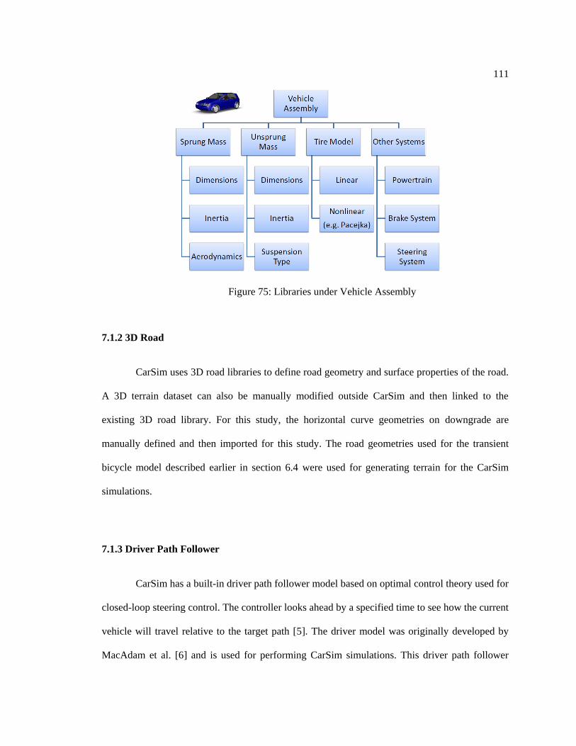
111
Figure 75: Libraries under Vehicle Assembly
7.1.2 3D Road
CarSim uses 3D road libraries to define road geometry and surface properties of the road.
A 3D terrain dataset can also be manually modified outside CarSim and then linked to the
existing 3D road library. For this study, the horizontal curve geometries on downgrade are
manually defined and then imported for this study. The road geometries used for the transient
bicycle model described earlier in section 6.4 were used for generating terrain for the CarSim
simulations.
7.1.3 Driver Path Follower
CarSim has a built-in driver path follower model based on optimal control theory used for
closed-loop steering control. The controller looks ahead by a specified time to see how the current
vehicle will travel relative to the target path [5]. The driver model was originally developed by
MacAdam et al. [6] and is used for performing CarSim simulations. This driver path follower

112
model with a 0.5 seconds preview time is used as steering control while performing the CarSim
simulations.
7.1.4 Speed Control
CarSim allows users to specify target speeds as a function of time or distance as shown in
Figure 76. It is difficult to control the speed of vehicle in CarSim using open-loop braking as the
CarSim braking system includes factors like ABS control and fluid dynamics time constants for
brake fluid. Hence, this thesis uses a built-in PID control in CarSim for tracking desired target
speed profiles. Also, since this study considers only constant decelerations, the target speed
profiles are linear. The speed, , of a vehicle obtained from bicycle model simulation is used as
target speed for CarSim speed controller.
Figure 76: Target speed vs. time for speed-controller in CarSim

113
7.2 CarSim Simulation Comparison
A simulation was performed for E-class SUV for stopping sight deceleration case using
transient bicycle model as well as CarSim. The vehicle applies brakes while traveling at 60 mph
speed on a curve with =4% and =-9%. Figure 77 shows the plots for vertical, longitudinal and
lateral forces acting on each axle of the vehicle using transient bicycle model and CarSim. The
transient bicycle model shows a good agreement with CarSim results except for the transients that
arise during braking at =15 seconds. This disagreement arises mainly because of using a steady-
state brake proportioning model and a simple linear tire model for transient bicycle model
simulations.
Figure 77: Per-axle forces for transient bicycle model and CarSim

114
Figure 78 shows the longitudinal friction factors for the bicycle model simulation and
CarSim simulation. The longitudinal friction demand from the transient bicycle model is different
from the CarSim simulation before the braking event. This is not significant since it is more
important to predict higher friction demand which occurs after the braking event. The steady-state
brake proportioning model predicts average value of friction demand reasonably well after the
braking event. The rear axle friction demand is higher than the front axle friction demand and
hence, it is the deciding factor in the friction demand versus friction supply analysis. The steady-
state brake proportioning model predicts longitudinal friction demand close to the CarSim results.
Figure 78: Longitudinal friction factor vs. time comparison
The bicycle model predicts higher maximum lateral friction demand for rear axle (0.18)
than the CarSim prediction (0.14) as seen in Figure 79. In order to show that the sudden
longitudinal weight transfer at braking is not the main reason for this difference, a simulation was
performed with a transfer function included accounting for the pitch dynamics of the vehicle. The
lateral friction demand for this case is shown in Figure 80. It can be seen that the effect of
longitudinal load transfer (pitch dynamics) on the lateral friction demand is negligible. Although

115
bicycle model has limitations, it gives close results when compared with the CarSim simulations,
if perhaps slightly conservative.
Figure 79: Lateral friction factor vs. time comparison
Figure 80: Lateral friction factor vs. time comparison (with pitch dynamics included)

116
References
1. CarSim, Mechanical Simulation Corporation, 2006. http://www.carsim.com
2. HVOSM, McHenry Software, 2006. http://www.mchenrysoftware.com
3. VDANL, Systems Technology Inc., 2006. http://www.systemstech.com
4. ADAMS, MSC Software, 2006. http://www.mscsoftware.com
5. PC-Crash, MEA Forensic Engineers and Scientists, 2006. http://www.maceng.com
6. MacAdam, C.C., Application of an Optimal Preview Control for Simulation of Closed-
Loop Automobile Driving, IEEE Transactions on Systems, Man, and Cybernetics, Vol.
11, June 1981

Chapter 8
Conclusions and Future Work
This chapter discusses the findings from the work in this thesis and suggests future work
that can be done to improve the analysis.
8.1 Conclusions
This study developed analytical and low-order simulation models for the horizontal curve
design analysis. It was observed that the vehicle parameters significantly affect the friction
demand of a vehicle going around a turn. The modified point mass model is independent of any
vehicle parameter and hence, it is unable to predict friction demands reasonably well. For
example, Figure 81 shows that the per-axle friction demands can be significantly different from
the net friction demand predicted by modified point mass model. In fact, the per-axle friction
demand is influenced by the vehicle parameters like CG height, CG position along vehicle‟s
length and brake-proportioning design.
In case of passenger cars, the rear-axle friction demand can be 40% higher than the front-
axle friction demand even for common braking cases. Hence, rear-axle friction demand is the
deciding factor while performing a friction demand versus friction supply analysis. Although the
rear-axle braking force is less than the front-axle in all cases, the normal load on rear axle is much
lower which causes the friction demand to increase and margin of safety to decrease. Since the
braking force requirement on rear-axle is lower, the brake proportioning model still operates at
brake application pressure, , less than ‟. Hence, unless the brake proportioning valve is load-

118
sensitive (which is usually not the case), the margins of safety can go below 0.1 at high speeds on
sharp curves with downgrades.
Figure 81: Lateral friction demand comparison ( =-9%, =9%, Stopping sight deceleration,
=60 mph, E-class SUV parameters)
Current horizontal curve design policy is mainly based on driver-comfort-based studies.
For such a design the margin of safety decreases as the design speed increases on wet roads as
seen in Figure 82. However, the margin of safety was found to be positive for passenger cars in
the event of stopping sight deceleration on all the grades. It was assumed that the stopping sight
distance is unaffected by the environmental conditions (like rain).
In case of emergency braking, even the steady-state model predicts a negative margin of
safety for E-class SUV for all road design variables. It must be noted that this prediction
corresponds to a worst case scenario and indicates that margin of safety can possibly go negative
for few seconds. A CarSim simulation was performed for emergency braking on a 9% downgrade
with an E-class SUV whose ABS controller is turned off. In Figure 83, it can be seen that the
vehicle shifts laterally by a lane-width from the time hits the brake until it comes to a stop for a
standard 12 feet lane-width design. Therefore, this might lead to a larger lane-width design for
horizontal curves on downgrades.

119
Figure 82: Steady-state bicycle model results for stopping sight deceleration
(E-class SUV, =-9%)
Figure 83: CarSim simulation for emergency braking on a 9% downgrade (ABS OFF, 0.5 seconds
driver preview time)
The rear-axle (peak) lateral friction demands for each model considered in this thesis are
shown in Figure 84. The overall trend indicates that as the transient model is the most

120
conservative model when compared with the multi-body simulations. Although the steady-state
bicycle model is also little conservative, it is not capable of handling transient maneuvers like
emergency lane-change maneuver described in this thesis. Hence, the transient bicycle model can
be a good choice for horizontal curve design.
Figure 84: Rear axle lateral friction demand comparison ( =-9%, =9%, Stopping sight
deceleration, =60 mph, E-class SUV parameters)
8.2 Future Work
8.2.1 Tire-pavement friction
The tire-pavement friction supply is a crucial factor in determining the margins of safety
for horizontal curve design. Friction measurements from the literature [1] were used for this
thesis for estimating tire-pavement friction supply. Although these measurements were presented
using a linear regression fit, the coefficient of friction on a wet road does not usually vary linearly
with the speed [2].

121
Also, friction measurements were recorded only for speeds of 40, 50, and 60 mph.
According to AASHTO the design speeds vary at an interval of 5 mph, and hence, the
measurements should be done at a 5 mph interval. Skid resistance measurements should be
performed at an interval of 5 mph at different sites. These sites should include asphalt as well as
concrete. The confidence intervals should be reported for each set of measurements. Also, skid
measurements on upgrades and downgrades will help to see if they significantly vary from the
friction measurements taken on a flat pavement. Skid measurements at different sections of a
single road segments will help to check for the homogeneity of friction supply within the
segment.
Modern skid measurement systems like the dynamic friction tester (DFT) measures skid
resistance up to 55 mph. For current highway design, the design speeds range up to 80 mph.
Hence, a physics-based tire model like LuGre model might be needed to find the friction supply
at higher design speeds. This will allow the friction demand versus friction supply analysis for
speeds above 60 mph.
Also, this thesis uses a linear tire model to predict the lateral tire forces. Ideally, a LuGre
model for wet roads should be used for lateral friction demand calculation.
8.2.2 Crash Data Analysis
Crash data on can help to identify concentration of crashes and then determine if they
occurred on sites with road geometry of interest, i.e. horizontal curves. Crash data for highways
can be obtained from different state departments of transportations for this purpose. Once such
data is obtained the relationship between margins of safety and crash statistics can be studied.

122
8.2.3 Road Geometries
This thesis assumes a constant superelevation rate for the tangent section and the curve
section. Typically a superelevation distribution is used to gradually transition from crown slope
on the tangent section to a full superelevation rate on the curve section. Road geometry should be
modeled in detail followed by comparing simulation results on these detailed geometries with the
simplified road geometries.
If field data is going to be used to validate the simulation, the road geometry of the curve
site should be measured. Primary measurements can include cross-slopes at different sections of
the curve. In order to record detailed road geometry, one can use an instrumented vehicle with
LIDAR to scan the road and to create digital terrain map of the road.
8.2.4 Speed Studies
This thesis used a curve entry deceleration on 0.85 m/s2 from Bonneson‟s study [3] to
represent typical driver behavior on the entry to a curve. Speed measurements for both passenger
cars and trucks will be helpful in order to calibrate analytical and simulation models. These
measurements will give statistics of typical speeds adopted by passenger cars and heavy trucks at
different segments of the curves on downgrade.
An instrumented vehicle can also be used for recording detailed speed profiles. The
instrumented vehicle will follow other vehicles starting at the tangent section of the road
throughout the curve section of the road. This manner of car-following experiment will provide
speed profiles of vehicles traveling on the curves which can be used in simulations.

123
8.2.5 Heavy Vehicles
This thesis only focused on the passenger car segment. The heavy vehicles like single-
unit trucks, tractor-semitrailer deserve particular attention while designing geometry of the roads.
Trucks have a much lower margin of safety on downgrades than a passenger car [3]. In this
thesis, it was observed that the margins of safety are very close to zero for stopping sight
deceleration case at 60 mph for passenger cars. Hence, a steady state model as well as a transient
vehicle model should be developed for heavy vehicles traveling on sharp curves with steep
grades, followed by a margin of safety analysis.
8.2.6 Low-Order Rollover Model
The transient vehicle model used in this study was developed for the per-axle skidding
analysis. The static rollover model developed in this thesis does not address transient maneuvers.
Heavy vehicles like trucks are known to exhibit lower values of rollover thresholds and hence, are
more susceptible to rollover. A low-order rollover model should be developed in order to predict
rollover or individual wheel lift events.

124
References
1. Flintsch, G.W. et al., Speed Adjustment Factors for Locked-Wheel Skid Trailer
Measurements, Transportation Research Record 2155, P. 117-13, Washington D.C., 2010
2. Wong, J.Y., Theory of Ground Vehicles, John Wiley and Sons, Inc. 2008
3. Bonneson, J.A., Side Friction and Speed as Controls for Horizontal Curve Design,
Journal of Transportation Engineering, Vol. 125, No. 6, American Society of Civil
Engineering, 1999
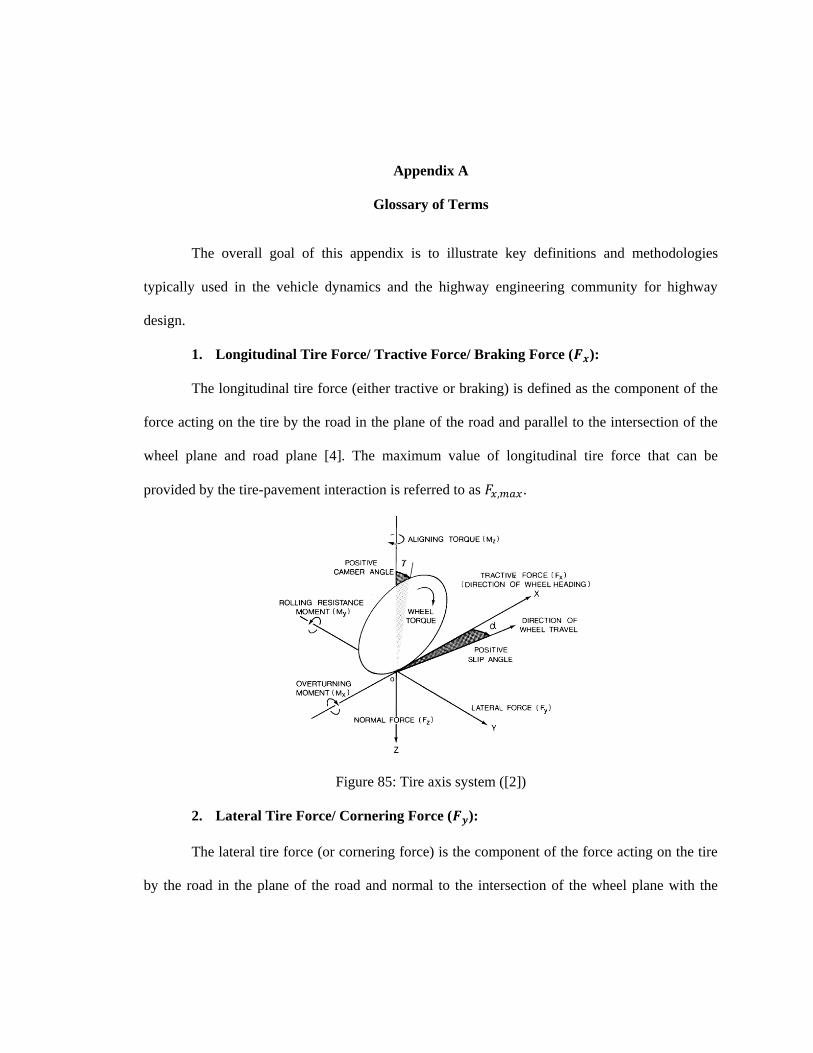
Appendix A
Glossary of Terms
The overall goal of this appendix is to illustrate key definitions and methodologies
typically used in the vehicle dynamics and the highway engineering community for highway
design.
1. Longitudinal Tire Force/ Tractive Force/ Braking Force ( ):
The longitudinal tire force (either tractive or braking) is defined as the component of the
force acting on the tire by the road in the plane of the road and parallel to the intersection of the
wheel plane and road plane [4]. The maximum value of longitudinal tire force that can be
provided by the tire-pavement interaction is referred to as .
Figure 85: Tire axis system ([2])
2. Lateral Tire Force/ Cornering Force ( ):
The lateral tire force (or cornering force) is the component of the force acting on the tire
by the road in the plane of the road and normal to the intersection of the wheel plane with the

126
road plane [4]. The maximum value of lateral tire force that can be provided by the tire-pavement
interaction is referred to as .
3. Side Friction Factor/ Side Friction Demand ( or ):
The side friction factor is the lateral tire force (Fy) divided by the vertical load (N) and is
represented by or .
The side friction factor also represents the friction demand created by lateral acceleration
that must be resisted or the vehicle will skid off the road.
4. Maximum Side Friction Supply ( ):
The maximum side friction supply is the maximum amount of side friction that can be
generated at the tire-pavement interface (to counteract lateral acceleration and prevent skidding).
This term is used by civil engineers, and it is unclear whether it is the same as the Peak Lateral
Coefficient of Road Adhesion or the Lateral Skid (or Sliding) Coefficient of Road Adhesion.
5. Design Side Friction Factor ( or ):
The maximum design side friction factor is the value of side friction factor corresponding
to the design speed and the minimum radius for a given superelevation rate as recommended by
the Green Book. This is set by AASHTO design policy. Note that this expression is not an actual
friction measurement.
The design side friction factor, is used to find minimum curve radius using the
simplified curve formula as shown in following equation:
In AASHTO‟s Green Book, this design side friction factor, is referred to as „side friction
factor‟ only.

127
6. Longitudinal Friction Factor/Demand ( ):
The longitudinal friction demand is the lateral tire force ( ) divided by the vertical load
( ) and is represented by .
7. Maximum Longitudinal Friction Supply ( ):
The maximum longitudinal friction supply is the maximum amount of longitudinal
friction that can be generated at the tire-pavement interface. This corresponds to the peak
coefficient of road adhesion ( ).
8. Peak Coefficient of Road Adhesion (or Friction) ( ):
The peak coefficient of road adhesion (or friction) ( ) is the maximum value of the ratio
of longitudinal force ( ) to the vertical load ( ). The same measurement can be obtained in the
lateral direction, in which case it is called the peak lateral coefficient of road adhesion.
9. Skid (or Sliding) Coefficient of Road Adhesion (or Friction) ( ):
Skid (or Sliding) coefficient of road adhesion (or friction) ( ) is the ratio of the
longitudinal force ( ) to the vertical load ( ) when the longitudinal slip is maximum (100%).
This is sometimes also called as skid resistance. Again, this can also be measured in the lateral
direction, in which case it is called the lateral skid coefficient of road adhesion.
10. Friction Ellipse:
The use of braking forces will reduce the available lateral friction, and the use of lateral
force will reduce the available braking forces. This interrelationship between lateral and
longitudinal forces is called the friction ellipse.
11. Friction Ellipse Equation:
The friction ellipse equation represents the operating range of tire forces and is given as
[2]:

128
(
)
(
)
Since friction factor is force divided by vertical load, a modified version of the friction
ellipse equation is given as [6]:
(
)
(
)
As long as value of “ ” is less than 1, the operating point (i.e. tire forces in longitudinal
& lateral directions) lies inside the friction ellipse and hence, the tire-pavement can generate
required friction force.
12. Friction Reserve:
The term “ ” in equations 9 and 10, can be referred to as the utilized amount of tire-
pavement friction or the measure of friction reserve. The friction reserve can be quantifies as
√ . One can usually infer that enough friction reserve is available as long as . When
, the friction reserve is exceeded.
13. Lateral Friction Supply ( ):
The lateral friction supply, , is available tire-pavement friction in the lateral
direction after satisfying the longitudinal friction demand.
√ (
)
14. Longitudinal Slip (λ):
The longitudinal slip (for braking) is defined as the ratio of longitudinal slip velocity
(which is the difference between the spin velocity of the braked tire and the spin velocity of the
straight free-rolling tire) to the spin velocity of the straight free-rolling tire. This ratio is generally
expressed as a percentage as follows (ref: [2]):

129
Where v is the linear speed of the tire center; is the rolling radius of the free-rolling
tire; ω is the angular speed of the tire. The resulting longitudinal slip number is dimensionless.
References:
1. American Association of State Highway and Transportation Officials, A Policy on
Geometric Design of Highways and Streets, Washington, D.C., 2004
2. Wong, J.Y., Theory of Ground Vehicles, John Wiley and Sons, Inc. 2008
3. Pacejka, H.B., Tire and Vehicle Dynamics, SAE International, 2006
4. Gillespie, T. Fundamentals of Vehicle Dynamics. SAE International Press, 1992
5. Milliken, W.F. and D.L. Milliken. Race Car Vehicle Dynamics, SAE International,
August 1995
6. Psarianos, B. et al. Influence of Vehicle parameters on Horizontal Curve Design of
Rural Highways, Transportation Research Circular E-C003, p. 22:1-10,
Transportation Research Board, 1998

Appendix B
Vehicle Family Parameters
Vehicle
Model
Vehicle Parameters (Metric Units)
(kg)
(kg-m2)
(m)
(m)
(m)
(m)
(m)
(rad/ )
(1/rad)
E-class
Sedan
1833 2765 1.414 1.634 0.567 1.600 0.107 0.093 23.754
E-class
SUV
1862 2488 1.247 1.704 0.670 1.575 0.005 0.073 13.827
Reference:
CarSim, Mechanical Simulation Corporation, 2006 http://www.carsim.com