Design of Maximum Power Point Tracker (MPPT) and … of Maximum Power Point Tracker (MPPT) and Phase ... despite that the solar irradiation and cell ... Four types of Maximum Power

Ofualagba Godswill, Onyan Aaron Okiemute, Igbinoba Kevwe Charles/ International Journal of Engineering

Research and Applications (IJERA) ISSN: 2248-9622 www.ijera.com

Vol. 2, Issue 3, May-Jun 2012, pp.1014-1025

1014 | P a g e

Design of Maximum Power Point Tracker (MPPT) and Phase

Locked Loop (PLL) in a PV-Inverter

Ofualagba Godswill 1*, Onyan Aaron Okiemute **, Igbinoba Kevwe Charles

*** * (Department of Electrical and Electronics Engineering, Federal University of Petroleum Resources, P.M.B. 1221,

Effurun, Delta State, Nigeria.)

** (Department of Electrical and Electronics Engineering, University of Benin, P.M.B. 1154, Benin City, Edo State,

Nigeria.)

*** (Department of Electrical and Electronics Engineering, University of Benin, P.M.B. 1154, Benin City, Edo

State, Nigeria)

ABSTRACT This paper deals with the design of the Maximum

Power Point Tracker (MPPT) and Phase Locked

Loop (PLL) controllers in a PV-Inverter. The

methods to optimizing the load of the PV module in

order to capture the highest amount of energy,

despite that the solar irradiation and cell

temperature never is constant. Four types of

Maximum Power Point Trackers (MPPT) have been

discussed and a novel MPPT algorithm has been

developed. The tracking of the fundamental grid

voltage, by means of a Phase Locked Loop (PLL)

was discussed. All the controllers have been

designed by standard design techniques, and

verified by simulation in MATLAB® /

SIMULINK® and PSIM®.

Keywords – Constant fill-factor, controllers,

incremental conductance, sweeping, tracking.

1. Introduction

The design of a power-electronic inverter depends on

many issues, such as silicon devices; magnetics;

capacitors; gate drives; grid performance; current-,

voltage- and temperature-sensing and -protection;

control strategies; and implementation, etc. This paper

discusses two of the controllers for a PV-Inverter, this

includes: Maximum Power Point Tracker (MPPT) for

the PV module, Phase Locked Loop (PLL) to track the

fundamental component of the grid voltage. There are

other controllers in a PV-Inverter but not discussed in

this paper. All the controllers needed in a PV-Inverter

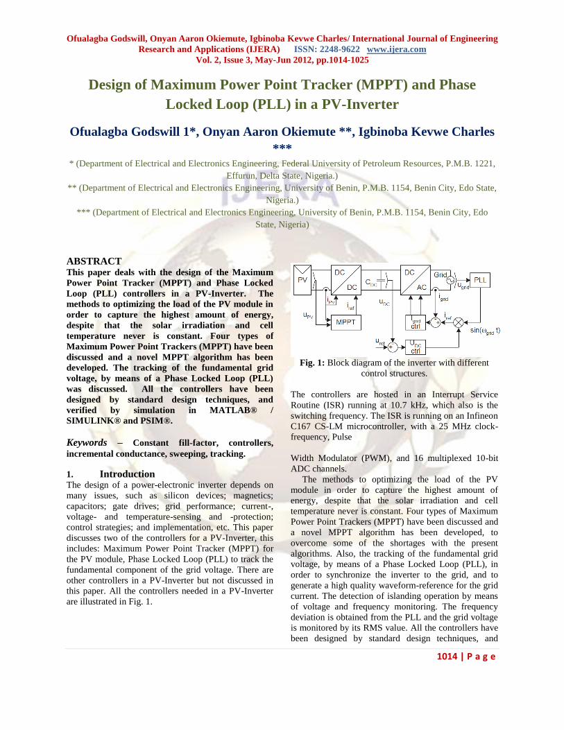
are illustrated in Fig. 1.

Fig. 1: Block diagram of the inverter with different

control structures.

The controllers are hosted in an Interrupt Service

Routine (ISR) running at 10.7 kHz, which also is the

switching frequency. The ISR is running on an Infineon

C167 CS-LM microcontroller, with a 25 MHz clock-

frequency, Pulse

Width Modulator (PWM), and 16 multiplexed 10-bit

ADC channels.

The methods to optimizing the load of the PV

module in order to capture the highest amount of

energy, despite that the solar irradiation and cell

temperature never is constant. Four types of Maximum

Power Point Trackers (MPPT) have been discussed and

a novel MPPT algorithm has been developed, to

overcome some of the shortages with the present

algorithms. Also, the tracking of the fundamental grid

voltage, by means of a Phase Locked Loop (PLL), in

order to synchronize the inverter to the grid, and to

generate a high quality waveform-reference for the grid

current. The detection of islanding operation by means

of voltage and frequency monitoring. The frequency

deviation is obtained from the PLL and the grid voltage

is monitored by its RMS value. All the controllers have

been designed by standard design techniques, and




1015 | P a g e

verified by simulation in MATLAB® / SIMULINK®

and PSIM®.

2. Maximum Power Point Tracker (MPPT) The operating point where the PV module generates the

most power is denoted the Maximum Power Point

(MPP) which co-ordinates are: UMPP, IMPP. The

available power from the PV module is a function of

solar irradiation, module temperature, and amount of

partial shadow. Thus, the MPP is never constant but

varies all the time. Sometimes it changes rapidly due to

fast changes in the weather conditions (The irradiance

can change as much as 500 W / (m2

s), or from zero to

bright sunlight in 2 seconds. This is measured during

springtime 2005 with a pyranometer). At other times, it

is fairly constant when no clouds are present. Four

major types of tracking algorithms (MPPT) are

available. They are (in order of complexity, simplest

first):

• Constant fill-factor (voltage or current)

• Sweeping

• Perturb and observe (hill-climbing)

• Incremental conductance

Other types of algorithms also exist, e.g. fuzzy-logic,

neural-networks, monitor/reference cells, etc. They are

however not reviewed here, due to their elevated

complexities, or the need for additional PV cells for

monitoring purpose.

2.1 Constant Fill-Factor

The constant fill-factor algorithms assume that the MPP

voltage is given as a constant fraction of the open

circuit module voltage, UOC, or that the MPP current is

given as a constant fraction of the short circuit module

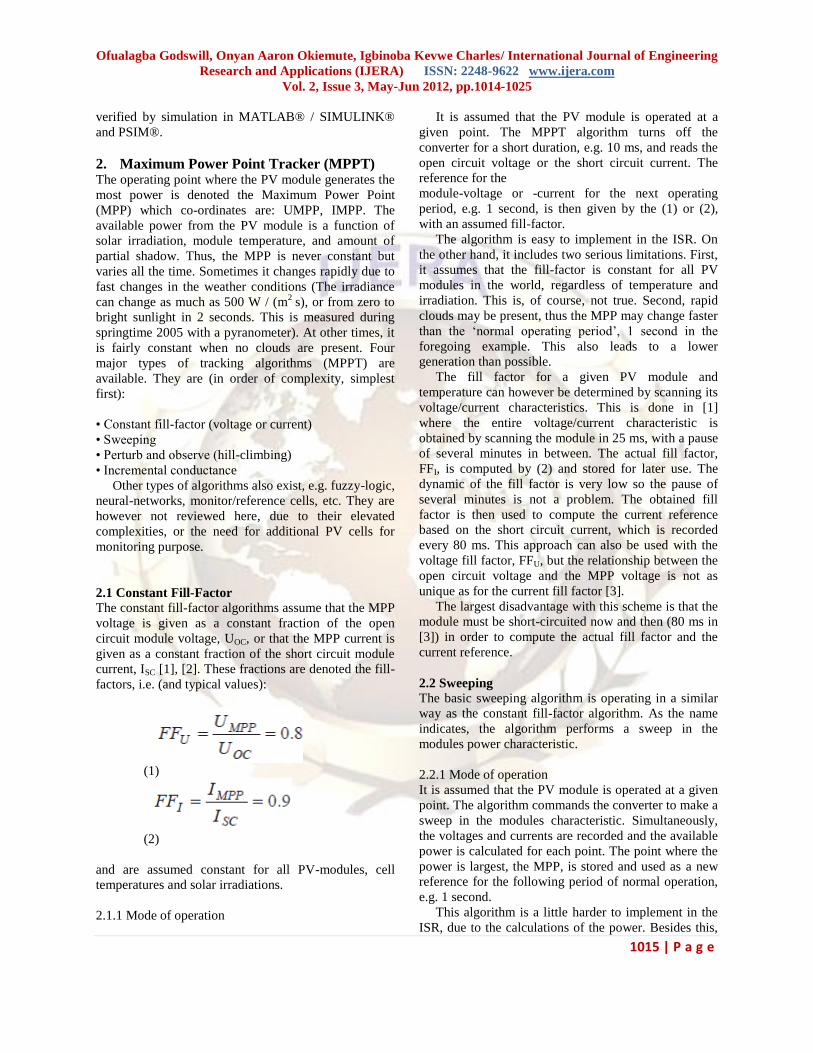
current, ISC [1], [2]. These fractions are denoted the fill-

factors, i.e. (and typical values):

(1)

(2)

and are assumed constant for all PV-modules, cell

temperatures and solar irradiations.

2.1.1 Mode of operation

It is assumed that the PV module is operated at a

given point. The MPPT algorithm turns off the

converter for a short duration, e.g. 10 ms, and reads the

open circuit voltage or the short circuit current. The

reference for the

module-voltage or -current for the next operating

period, e.g. 1 second, is then given by the (1) or (2),

with an assumed fill-factor.

The algorithm is easy to implement in the ISR. On

the other hand, it includes two serious limitations. First,

it assumes that the fill-factor is constant for all PV

modules in the world, regardless of temperature and

irradiation. This is, of course, not true. Second, rapid

clouds may be present, thus the MPP may change faster

than the ‘normal operating period’, 1 second in the

foregoing example. This also leads to a lower

generation than possible.

The fill factor for a given PV module and

temperature can however be determined by scanning its

voltage/current characteristics. This is done in [1]

where the entire voltage/current characteristic is

obtained by scanning the module in 25 ms, with a pause

of several minutes in between. The actual fill factor,

FFI, is computed by (2) and stored for later use. The

dynamic of the fill factor is very low so the pause of

several minutes is not a problem. The obtained fill

factor is then used to compute the current reference

based on the short circuit current, which is recorded

every 80 ms. This approach can also be used with the

voltage fill factor, FFU, but the relationship between the

open circuit voltage and the MPP voltage is not as

unique as for the current fill factor [3].

The largest disadvantage with this scheme is that the

module must be short-circuited now and then (80 ms in

[3]) in order to compute the actual fill factor and the

current reference.

2.2 Sweeping

The basic sweeping algorithm is operating in a similar

way as the constant fill-factor algorithm. As the name

indicates, the algorithm performs a sweep in the

modules power characteristic.


It is assumed that the PV module is operated at a given

point. The algorithm commands the converter to make a

sweep in the modules characteristic. Simultaneously,

the voltages and currents are recorded and the available

power is calculated for each point. The point where the

power is largest, the MPP, is stored and used as a new

reference for the following period of normal operation,

e.g. 1 second.

This algorithm is a little harder to implement in the

ISR, due to the calculations of the power. Besides this,




1016 | P a g e

it must also include a comparator function in order to

locate the MPP. The basic sweeping algorithm suffers

from the same limitation as the constant fill-factor

algorithm: Rapid clouds may be present, thus the MPP

may change faster than the ‘normal operating period’.

Besides, if the sweep-duration is too long, the

irradiance may have changed and the recorded curve

corresponds to two different irradiations. This can be

mitigated by starting the sweep at zero voltage, i.e.

measuring the actual short circuit current. The sweep is

then continued to open circuit conditions while all the

different operating points are investigated for available

power. Finally, the module is short circuited again and

the new short-circuit currents are measured. Following,

the irradiance has changed if the measured short-circuit

currents do not agree with each other, and nothing can

really be stated about the location of the MPP.

2.3 Perturb and Observer

The perturb-and-observe algorithm is also known as the

‘climbing hill’ approach. The reference is constantly

changed, and the resulting power is compared with the

previous power, and a decision about the direction of

MPP can thus be stated [4].



point. The voltage reference of the PV module is

initialized to UPV *[n]. After the reference has been

reached, the generated power PPV[n] is calculated and

stored. The reference is then changed to UPV*[n+1], and

the generated power, PPV[n+1], is computed and stored.

If PPV[n] > PPV[n+1], the MPP is located in the opposite

direction of which the reference was changed. Thus, the

new reference should be equal to: UPV*[n+2] =

UPV*[n+1] - ∆U. In the opposite case where PPV[n] <

PPV[n+1], the MPP is located in the same direction as

the change in the reference, and the new reference

should be in the same direction: UPV *[n+2] =

UPV*[n+1] + ∆U.

This way of searching in the MPP is fast when the

irradiance is constant. On the other hand, it includes

some limitations. First, the generated power is

fluctuating around the MPP, while the PV voltage is

alternating around the MPP. Making ∆U sufficiently

small can mitigate this. However, this is on the cost of

increasing the searching time when large variation in

the irradiance is present. It is preferred to make ∆U

large to catch the MPP during rapid changes, since the

power loss due to the oscillations around the MPP is

small. A large ∆U also enhances the signal-to-noise

ratio in the sensed current.

Second, rapidly changing in the irradiation can lead

to a wrong decision about the direction of the MPP [5].

This can however be solved by introducing a third

reference, UPV*[n+3], [6], [7]. Another solution is to

ensure that the change in power as function of the

change in the voltage-reference always is larger than

the change in power due to change in radiation [8].

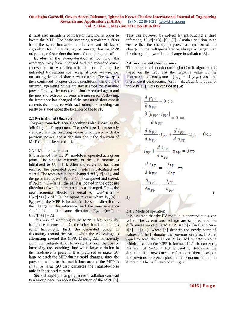
2.4 Incremental Conductance

The incremental conductance (IndCond) algorithm is

based on the fact that the negative value of the

instantaneous conductance (-sPV = -iPV/uPV) and the

incremental conductance (dsPV = diPV/duPV), is equal at

the MPP [5]. This is verified in (3):

(

3)



point. The current and voltage are sampled and the

differences are calculated as: ∆i = i[n] - i[n-1] and ∆u =

u[n] - u[n-1], where [n] denotes the newly sampled

values and [n-1] denotes the previous samples. If ∆u is

equal to zero, the sign on ∆i is used to determine in

which direction the MPP is located. If ∆u is non-zero,

the sign of ∆i/∆u + I/U is used to determine the

direction. The new current reference is then based on

the previous reference plus the information about the

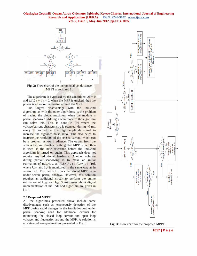
direction. This is illustrated in Fig. 2.




1017 | P a g e

Fig. 2: Flow chart of the incremental conductance

MPPT algorithm [5].

The algorithm is bypassed by the conditions: ∆i = 0

and ∆i/ ∆u + i/u = 0, when the MPP is tracked, thus the

power is no more fluctuating around the MPP.

The largest disadvantage with the IndCond

algorithm, as with the other algorithms, is the problem

of tracing the global maximum when the module is

partial shadowed. Adding a scan mode to the algorithm

can solve this. This is done in [9] where the

voltage/current characteristic is scanned, during 40 ms,

every 12 second, with a high amplitude signal to

increase the signal-to-noise ratio. This also helps to

increase the resolution of the sensed current, which can

be a problem at low irradiance. The output from the

scan is the co-ordinates for the global MPP, which then

is used as the new reference before the IndCond

algorithm is turned on again. This approach does not

require any additional hardware. Another solution

during partial shadowing is to make an initial

estimation of uMPP/iMPP as (0.8×UOC) / (0.9×ISC) [10],

where UOC and ISC is monitored in the same way as in

section 2.1. This helps to track the global MPP, even

under severe partial shadow. However, this solution

requires an additional circuit to perform the online

estimation of UOC and ISC. Some issues about digital

implementation of the IndCond algorithm are given in

[11].

2.5 Proposed MPPT

All the algorithms presented above include some

disadvantages such as: erroneously detection of the

MPP during rapid changes in the irradiation and under

partial shadow; need for additional circuits for

monitoring the closed loop current and open loop

voltage; and fluctuation around the MPP. A solution is

an extended sweep algorithm, presented in Fig. 3.

Fig. 3: Flow chart for the proposed MPPT.




1018 | P a g e



point. While this is on-going, the algorithm is

monitoring the instantaneous module voltage, which

should be equal to the recorded MPP voltage. Due to

changes in temperature and/or irradiation, the

instantaneous voltage will also change if the current is

kept constant. Thus, instead of performing a new sweep

every 10th

second or so, a new sweep is only initialized

when the module voltage has changed more than ∆U

from the original MPP voltage. Moreover, the sweeping

range is necessarily not equal to the entire module

current range (from open circuit operation to the short

circuit operation), but could be a fraction of the original

MPP current, e.g. ∆I. This ensures a fast sweep, where

only a little energy is lost.

The size of ∆U to start a new sweep is a tradeoff

between power lost due to deviation from the real MPP

during monitoring, and stability of the algorithm, i.e.

how often the characteristic is swept. The change in the

voltage across the module, ∆uPV, when the input current

to the DC-DC converter is constant and the short circuit

current is changed by an amount of ∆iSC, is:

(4)

when operated in the nearby region of the MPP. The

threshold value to initiate a new sweep is set to 3% of

the actual MPP current, which involves that sweep-

mode is entered when the voltage has changed more

than 3% from the previous MPP voltage.

The sweeping range is merely selected to be equal to

0.90×IMPP to 1.05×IMPP, but is increased by additional

0.03 if the recorded power in the last sweeping-point

exceeds the power in the next-last point. This is done to

ensure that the MPP always will be tracked during the

sweep. An Under-Voltage-Lock-Out (UVLO) is also

included in the algorithm, not illustrated in Fig. 3,

which decreases the current reference to 0.90 if the PV

module voltage decreases below 20.0 V and starts the

sweeping mode. This is to ensure than the voltage never

collapses.

Finally, the algorithm must be able to follow the

maximum rate-of-change-of-current, disc/dt, in order to

track the MPP during rapid changes in the irradiation.

The rate-of-change-of-current is proportional to the

rate-of-change-of-irradiation, which is assumed to have

a maximum value of 1000 W/(m2×s)

6. The STC short

circuit current for modules is measured at 1000 W/m2.

Thus, the duration of the sweep, from zero-current and

until the module voltage reached a predefined

minimum, should not be larger than 1 second.

2.6 Simulated Results

The proposed MPPT algorithm is simulated in

MATLAB/SIMULINK. The models of the PV module

and the DC-DC converter are implemented in

SIMULINK, together with the MPPT algorithm. The

algorithm is programmed in C-code and compiled into

an s-function for SIMULINK. The model of the PV

module is based on the Shell Ultra175 module, operated

at various irradiations but constant cell temperature.

The temperature is kept constant, in order to make a

simple prediction of the maximum available power for

a given amount of irradiation.

The following is applied to all simulations: The

function generating the normal distribution irradiation

is sampled every 0.5s. The output from the normal

distribution generator is multiplied with a noise-signal

with mean 1.0 and variance (0.01/3)2 (corresponds to a

signal within the range from approx. 0.99 to 1.01).

Finally, the irradiance is rate-limited to ± 1000

W/(m2×s), in order to keep realistic rate-of-change-of-

irradiance.

A simulation of increasing and decreasing

irradiation is depicted in Fig. 4. Another set of eight

simulations, with two different mean irradiations and

four different variances are also made in order to

evaluate the steady state efficiency of the MPPT

algorithm at low and high irradiation. The results are

presented in TABLE 1.




1019 | P a g e

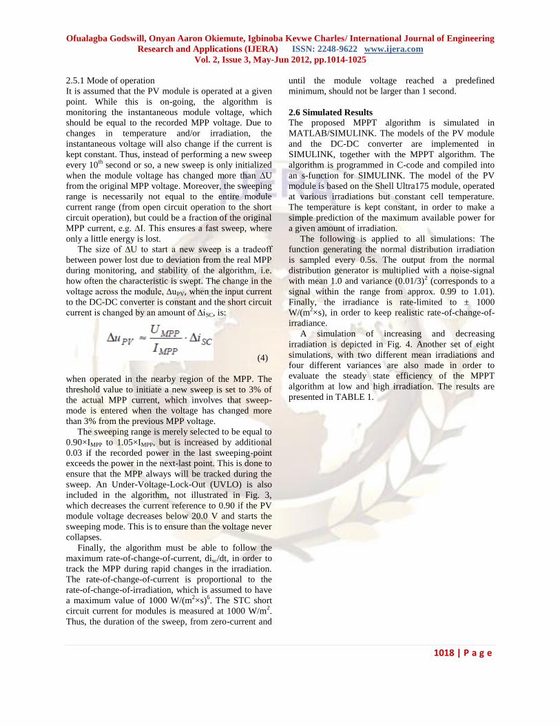
Fig. 4: Simulated results for the proposed MPPT

algorithm.

The total efficiency is evaluated to 98.0%. From top

and down: 1) Upper is shown the amount of solar

irradiation. The high-level irradiation is defined in the

span from 990 W/m2 to 1140 W/m2 in the time span

from 3.0s to 7.0s. The low-level irradiation is

approximately 60 W/m2. 2) Voltage across the PV

module. 3) Current drawn from the PV module. 4)

Power generated by the PV module.

The total MPPT efficiency (simulated) in Fig. 4 is

evaluated to 98.0%, and can be broken down to the

following intervals (PPV/PMPP):

• Low irradiation (approx. 60 W/m2): 28.5 J /

30.2 J = 94.3%,

• Increasing irradiation: 92.7 J /

99.5 J = 93.2%,

• High irradiation (approx. 1100 W/m2): 741 J / 748

J = 99.1%,

• Decreasing irradiation: 92.4 J /

96.6 J = 95.7%.

This shows that the efficiency is good; both for low,

high, increasing and decreasing irradiation.

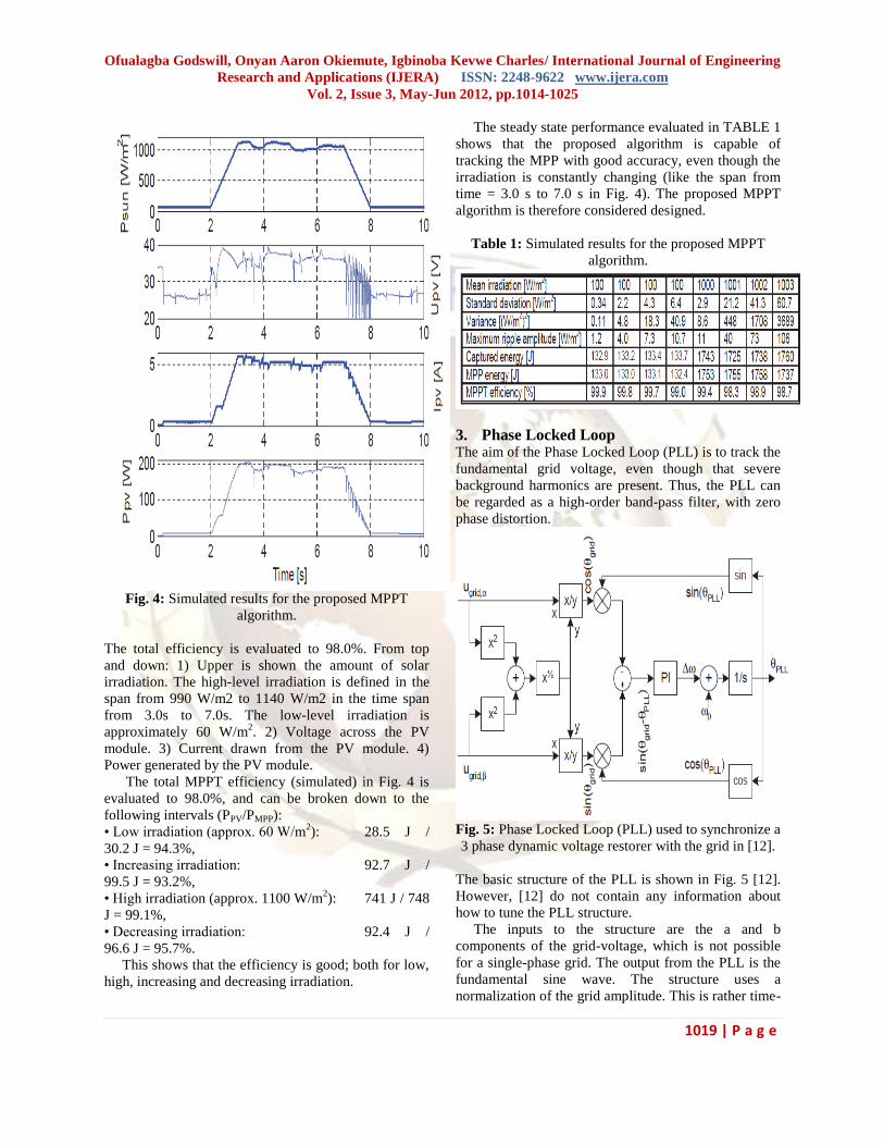
The steady state performance evaluated in TABLE 1

shows that the proposed algorithm is capable of

tracking the MPP with good accuracy, even though the

irradiation is constantly changing (like the span from

time = 3.0 s to 7.0 s in Fig. 4). The proposed MPPT

algorithm is therefore considered designed.

Table 1: Simulated results for the proposed MPPT

algorithm.

3. Phase Locked Loop The aim of the Phase Locked Loop (PLL) is to track the

fundamental grid voltage, even though that severe

background harmonics are present. Thus, the PLL can

be regarded as a high-order band-pass filter, with zero

phase distortion.

Fig. 5: Phase Locked Loop (PLL) used to synchronize a

3 phase dynamic voltage restorer with the grid in [12].

The basic structure of the PLL is shown in Fig. 5 [12].

However, [12] do not contain any information about

how to tune the PLL structure.

The inputs to the structure are the a and b

components of the grid-voltage, which is not possible

for a single-phase grid. The output from the PLL is the

fundamental sine wave. The structure uses a

normalization of the grid amplitude. This is rather time-




1020 | P a g e

consuming in the ISR, since it requires two

multiplications, two divisions and a square-root

operation. This is not necessary, since the amplitude is

otherwise just included as a part of the proportional

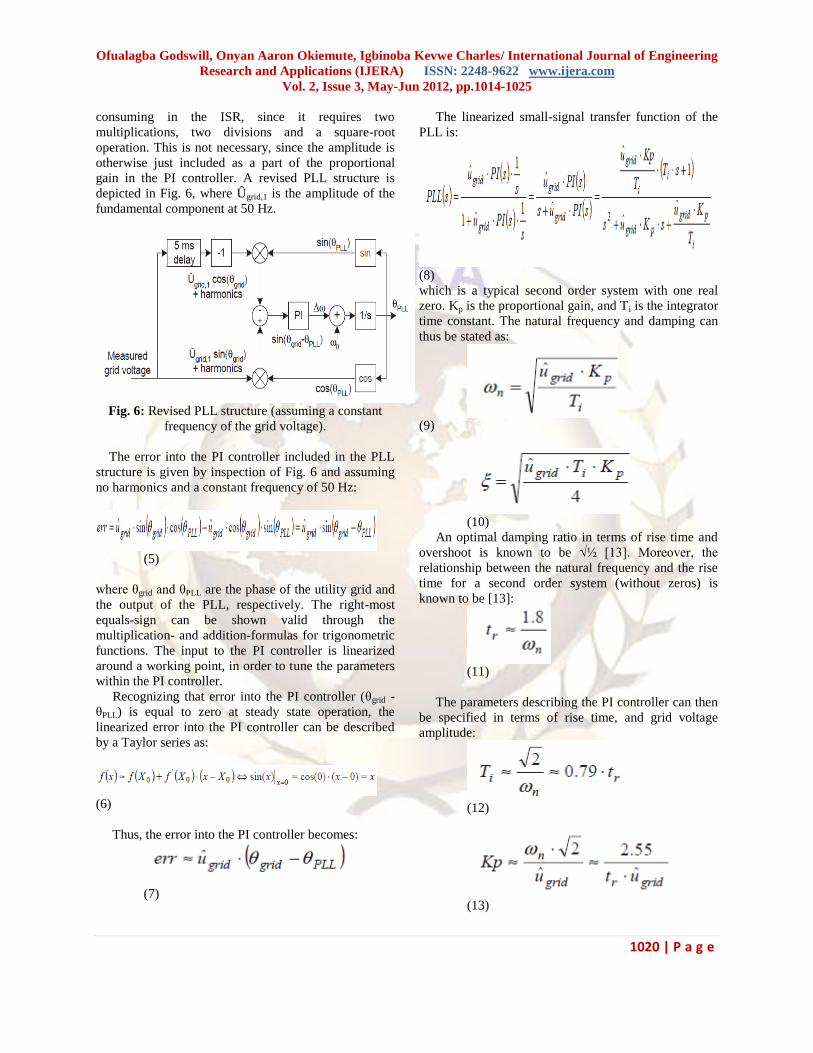
gain in the PI controller. A revised PLL structure is

depicted in Fig. 6, where Ûgrid,1 is the amplitude of the

fundamental component at 50 Hz.

Fig. 6: Revised PLL structure (assuming a constant

frequency of the grid voltage).

The error into the PI controller included in the PLL

structure is given by inspection of Fig. 6 and assuming

no harmonics and a constant frequency of 50 Hz:

(5)

where θgrid and θPLL are the phase of the utility grid and

the output of the PLL, respectively. The right-most

equals-sign can be shown valid through the

multiplication- and addition-formulas for trigonometric

functions. The input to the PI controller is linearized

around a working point, in order to tune the parameters

within the PI controller.

Recognizing that error into the PI controller (θgrid -

θPLL) is equal to zero at steady state operation, the

linearized error into the PI controller can be described

by a Taylor series as:

(6)

Thus, the error into the PI controller becomes:

(7)

The linearized small-signal transfer function of the

PLL is:

(8)

which is a typical second order system with one real

zero. Kp is the proportional gain, and Ti is the integrator

time constant. The natural frequency and damping can

thus be stated as:

(9)

(10)

An optimal damping ratio in terms of rise time and

overshoot is known to be √½ [13]. Moreover, the

relationship between the natural frequency and the rise

time for a second order system (without zeros) is

known to be [13]:

(11)

The parameters describing the PI controller can then

be specified in terms of rise time, and grid voltage

amplitude:

(12)

(13)




1021 | P a g e

For a rise time of 10 ms, with optimal damping and

European systems, the parameters of the PI controller

equals: Kp = 0.78, and Ti = 7.9×10-3

. A Bode plot is

shown in Fig. 7 for different values of the amplitude of

the grid voltage, ûgrid, and fixed controller parameters.

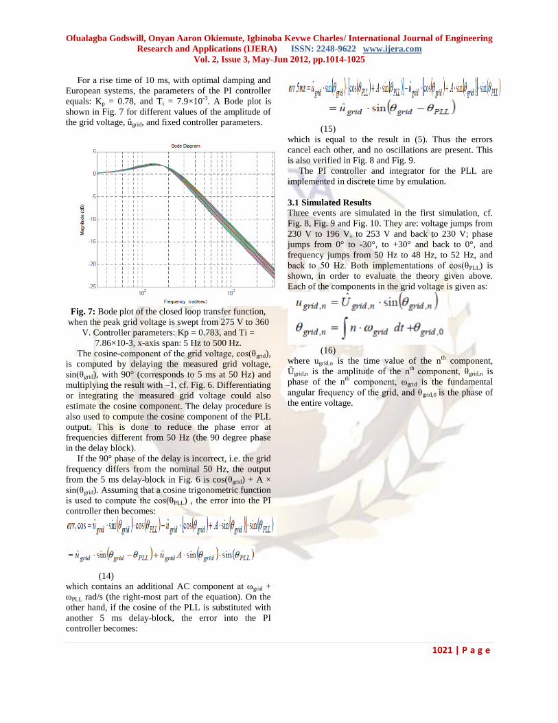
Fig. 7: Bode plot of the closed loop transfer function,

when the peak grid voltage is swept from 275 V to 360

V. Controller parameters: Kp = 0.783, and Ti =

7.86×10-3, x-axis span: 5 Hz to 500 Hz.

The cosine-component of the grid voltage, cos(θgrid),

is computed by delaying the measured grid voltage,

sin(θgrid), with 90° (corresponds to 5 ms at 50 Hz) and

multiplying the result with –1, cf. Fig. 6. Differentiating

or integrating the measured grid voltage could also

estimate the cosine component. The delay procedure is

also used to compute the cosine component of the PLL

output. This is done to reduce the phase error at

frequencies different from 50 Hz (the 90 degree phase

in the delay block).

If the 90° phase of the delay is incorrect, i.e. the grid

frequency differs from the nominal 50 Hz, the output

from the 5 ms delay-block in Fig. 6 is cos(θgrid) + A ×

sin(θgrid). Assuming that a cosine trigonometric function

is used to compute the cos(θPLL) , the error into the PI

controller then becomes:

(14)

which contains an additional AC component at ωgrid +

ωPLL rad/s (the right-most part of the equation). On the

other hand, if the cosine of the PLL is substituted with

another 5 ms delay-block, the error into the PI

controller becomes:

(15)

which is equal to the result in (5). Thus the errors

cancel each other, and no oscillations are present. This

is also verified in Fig. 8 and Fig. 9.

The PI controller and integrator for the PLL are

implemented in discrete time by emulation.

3.1 Simulated Results

Three events are simulated in the first simulation, cf.

Fig. 8, Fig. 9 and Fig. 10. They are: voltage jumps from

230 V to 196 V, to 253 V and back to 230 V; phase

jumps from 0° to -30°, to +30° and back to 0°, and

frequency jumps from 50 Hz to 48 Hz, to 52 Hz, and

back to 50 Hz. Both implementations of cos(θPLL) is

shown, in order to evaluate the theory given above.

Each of the components in the grid voltage is given as:

(16)

where ugrid,n is the time value of the nth

component,

Ûgrid,n is the amplitude of the nth

component, θgrid,n is

phase of the nth

component, ωgrid is the fundamental

angular frequency of the grid, and θgrid,0 is the phase of

the entire voltage.




1022 | P a g e

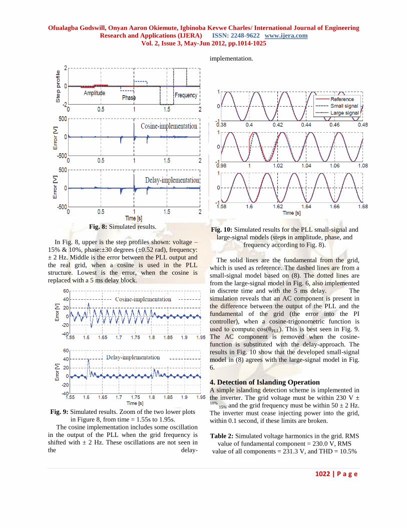
Fig. 8: Simulated results.

In Fig. 8, upper is the step profiles shown: voltage –

15% & 10%, phase:±30 degrees (±0.52 rad), frequency:

± 2 Hz. Middle is the error between the PLL output and

the real grid, when a cosine is used in the PLL

structure. Lowest is the error, when the cosine is

replaced with a 5 ms delay block.

Fig. 9: Simulated results. Zoom of the two lower plots

in Figure 8, from time = 1.55s to 1.95s.

The cosine implementation includes some oscillation

in the output of the PLL when the grid frequency is

shifted with ± 2 Hz. These oscillations are not seen in

the delay-

implementation.

Fig. 10: Simulated results for the PLL small-signal and

large-signal models (steps in amplitude, phase, and

frequency according to Fig. 8).

The solid lines are the fundamental from the grid,

which is used as reference. The dashed lines are from a

small-signal model based on (8). The dotted lines are

from the large-signal model in Fig. 6, also implemented

in discrete time and with the 5 ms delay. The

simulation reveals that an AC component is present in

the difference between the output of the PLL and the

fundamental of the grid (the error into the PI

controller), when a cosine-trigonometric function is

used to compute cos(θPLL). This is best seen in Fig. 9.

The AC component is removed when the cosine-

function is substituted with the delay-approach. The

results in Fig. 10 show that the developed small-signal

model in (8) agrees with the large-signal model in Fig.

6.

4. Detection of Islanding Operation A simple islanding detection scheme is implemented in

the inverter. The grid voltage must be within 230 V ± 10%

15% and the grid frequency must be within 50 ± 2 Hz.

The inverter must cease injecting power into the grid,

within 0.1 second, if these limits are broken.

Table 2: Simulated voltage harmonics in the grid. RMS

value of fundamental component = 230.0 V, RMS

value of all components = 231.3 V, and THD = 10.5%




1023 | P a g e

The grid voltage can be monitored in many different

ways: Average of the absolute grid voltage, Root

Means Square (RMS) of the grid voltage, amplitude

detection of the grid voltage by using the sin2(x) +

cos2(x) = 1 relationship, and Fourier sine-transform of

the grid voltage:

(17)

(18)

(19)

(20)

Simulations are used to evaluate all four algorithms.

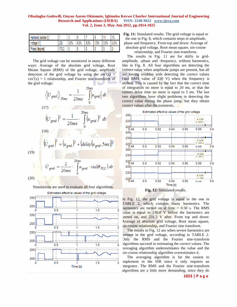
Fig. 11: Simulated results. The grid voltage is equal to

the one in Fig. 8, which contains steps in amplitude,

phase and frequency. From top and down: Average of

absolute grid voltage, Root mean square, sin-cosine

relationship, and Fourier sine-transform.

The results in Fig. 11 are for shifts in grid-

amplitude, -phase and -frequency, without harmonics,

like in Fig. 8. All four algorithms are detecting the

correct value when amplitude jumps are present, but all

are having troubles with detecting the correct values

(and RMS value of 230 V) when the frequency is

shifted. This is caused by the fact that the correct time

of integration no more is equal to 20 ms, or that the

correct delay time no more is equal to 5 ms. The last

two algorithms have slight problems in detecting the

correct value during the phase jump, but they obtain

correct values after the transients.

Fig. 12: Simulated results.

In Fig. 12, the grid voltage is equal to the one in

TABLE 2, which contains many harmonics. The

harmonics are turned on at time = 0.50 s. The RMS

value is equal to 230.0 V before the harmonics are

turned on, and 231.3 V after. From top and down:

Average of absolute grid voltage, Root mean square,

sin-cosine relationship, and Fourier sine transform.

The results in Fig. 12 are when severe harmonics are

present in the grid voltage, according to TABLE 2.

Only the RMS and the Fourier sine-transform

algorithms succeed in estimating the correct values. The

averaging algorithm underestimates the value and the

sin-cosine relationship algorithm overestimates it.

The averaging algorithm is far the easiest to

implement in the ISR since it only requires an

integrator. The RMS and the Fourier sine-transform

algorithms are a little more demanding, since they do




1024 | P a g e

also require a multiplication of two time-varying

signals. Finally, the sin-cosine relationship algorithm

requires a 5 ms delay of the sampled signal and two

multiplications (the delay is already included in the

PLL), or a 5 ms delay of the sampled signal, raised to

the second power (not included in the PLL). Taking all

these issues into consideration, the RMS algorithm

seems to be the best candidate for detecting the level of

voltage, both in term of precision and implementation.

The frequency of the grid is monitored by the output

of the PI controller included in the PLL structure. The

output of the PI controller is equal to the difference

between the actual frequency and the nominal

frequency (ω0 in Fig. 6). The output from the

calculation of the RMS value of the grid voltage, and

the output from the PI controller are both fed to a

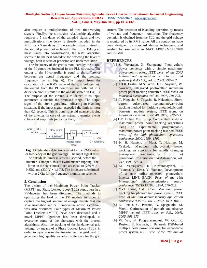
detection circuit similar to the one illustrated in Fig. 13.

The purpose of the circuit is to detect if its input

parameter is outside the premised range. The output

signal of the circuit goes low, indicating an islanding

situation, if the input signal exceeded the limit in more

than 0.1 second. This is done to avoid nuance tripping

of the inverter, in case of the normal dynamics events

(phase and amplitude jumps) in the grid.

Fig. 13: Islanding detection circuit for the RMS value

or frequency of the grid voltage. The input signal must

be outside its limits in least 0.1 second, before the

inverter is stopped, this to avoid nuance tripping. The

limits in the right-most block are equal to (230 V ×

0.85)2 and (230 V × 1.10)2. The limits are substituted

with ± 2×2π for the frequency monitoring scheme.

5. Conclusion The design of the Maximum Power Point Tracker

(MPPT) and Phase Locked Loop (PLL) controllers in a

PV-Inverter has been discussed. The methods to

optimizing the load of the PV module in order to

capture the highest amount of energy despite that the

solar irradiation and cell temperature never is constant

was also discussed. Four types of Maximum Power

Point Trackers (MPPT) have been discussed and a

novel MPPT algorithm has been developed, to

overcome some of the shortages with the present

algorithms. Also, the tracking of the fundamental grid

voltage, by means of a Phase Locked Loop (PLL), in

order to synchronize the inverter to the grid, and to

generate a high quality waveform-reference for the grid

current. The detection of islanding operation by means

of voltage and frequency monitoring. The frequency

deviation is obtained from the PLL and the grid voltage

is monitored by its RMS value. All the controllers have

been designed by standard design techniques, and

verified by simulation in MATLAB®/SIMULINK®

and PSIM®.

REFERENCES [1] S. Yuvarajan, X. Shanguang, Photo-voltaic

power converter with a simple maximum-

power-point-tracker, IEEE proc. of the 2003

international symposium on circuits and

systems (ISCAS '03), vol. 3, 2003, 399-402.

[2] J.H.R Enslin, M.S. Wolf, D.B. Snyman, W.

Swiegers, Integrated photovoltaic maximum

power point tracking converter, IEEE trans. on

industrial electronics, vol. 44, 1997, 769-773.

[3] T. Noguchi, S. Togashi, R. Nakamoto, Short-

current pulse-based maximumpower-point

tracking method for multiple photovoltaic-and-

converter module system, IEEE trans. on

industrial electronics, vol. 49, 2002, 217-223.

[4] D.P. Hohm, M.E. Ropp, Comparative study of

maximum power point tracking algorithms

using an experimental, programmable,

maximum power point tracking test bed, IEEE

proc. of the 28th photovoltaic specialists

conference, 2000, 1699- 1702.

[5] K. H. Hussein, I. Muta, T. Hoshino, M.

Osakada, Maximum photovoltaic power

tracking: an algorithm for rapidly changing

atmospheric conditions, IEE proc. of

generation, transmission and distribution, vol.

142, 1995, 59-64.

[6] M. Yamaguchi, K. Kawarabayashi, T.

Takuma, Y. Ueda, Y. Yamano, Development

of a new utility-connected photovoltaic

inverter LINE BACK, Proc. of the 16th

international telecommunications energy

conference (INTELEC'94), 1994, 676-682.

[7] Y.-T. Hsiao, C.-H. Chen, Maximum power

tracking for photovoltaic power system, IEEE

proc. of the 37th annual industry application

conference (IAS’02), vol. 2, 2002, 1035-1040.

[8] N. Femia, G. Petrone, G. Spagnuolo, M.

Vitelli, Optimization of perturb and observe

MPPT method, IEEE trans. on P.E., 20(4),

2005, 963-973.

[9] W. Wu, N. Pongratananukul, W. Qiu, K.

Rustom, K. Kasparis, I. Batarseh, DSP-based

multiple peak power tracking for expandable

power system, IEEE proc. of the 18th annual




1025 | P a g e

applied power electronics conference and

exposition (APEC'03), vol. 1, 2003, 525-530.

[10] K. Kobayashi, I. Takano, Y. Sawada, A study

on a two stage maximum power point tracking

control of a photovoltaic system under

partially shaded isolation conditions, IEEE

proc. of the power engineering society general

meeting, vol. 4, 2003, 2612-2617.

[11]T.-Y. Kim, H.-G. Ahn, S. K. Park, Y.-K. Lee,

A novel maximum power point tracking

control for photovoltaic power system under

rapidly changing solar radiation, IEEE proc. of

the international symposium on industrial

electronics (ISIE’01), vol. 2 , 2001, 1011-

1014.

[12] J.G. Nielsen, Design and Control of a

Dynamic Voltage Restorer, Ph.D. thesis,

Institute of Energy Technology, Aalborg

University, 2002.

[13] G.F. Franklin, J.D. Powell, A. Emami-Naeini,

Feedback control of dynamic systems 3rd

edition, (Addison Wesley) ISBN: 0-201-

53487-8.

[14] S.B. Kjaer, Design and Control of an Inverter

for Photovoltaic Applications, Ph.D. thesis,

Institute of Energy Technology, Aalborg

University, 2005.

Documents

Design of Maximum Power Point Tracker (MPPT) and … of Maximum Power Point Tracker (MPPT) and Phase ... despite that the solar irradiation and cell ... Four types of Maximum Power