Embed Size (px)
Citation preview

Design of optimal Runge-Kutta methods
David I. Ketcheson
King Abdullah University of Science & Technology(KAUST)
D. Ketcheson (KAUST) 1 / 36

Acknowledgments
Some parts of this are joint work with:
Aron Ahmadia
Matteo Parsani
D. Ketcheson (KAUST) 2 / 36

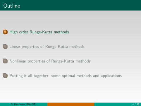
Outline
1 High order Runge-Kutta methods
2 Linear properties of Runge-Kutta methods
3 Nonlinear properties of Runge-Kutta methods
4 Putting it all together: some optimal methods and applications
D. Ketcheson (KAUST) 3 / 36
Outline
1 High order Runge-Kutta methods
2 Linear properties of Runge-Kutta methods
3 Nonlinear properties of Runge-Kutta methods
4 Putting it all together: some optimal methods and applications
D. Ketcheson (KAUST) 4 / 36
Solution of hyperbolic PDEs
The fundamental algorithmic barrier is the CFL condition:
∆t ≤ a∆x
Implicit methods don’t usually help (due to reduced accuracy)
Strong scaling limits the effectiveness of spatial parallelism alone
Strategy: keep ∆x as large as possible by using high order methods
But: high order methods cost more and require more memory
Can we develop high order methods that are as efficient as lowerorder methods?
D. Ketcheson (KAUST) 5 / 36
Time Integration
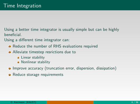
Using a better time integrator is usually simple but can be highlybeneficial.
Using a different time integrator can:
Reduce the number of RHS evaluations required
Alleviate timestep resrictions due to
Linear stabilityNonlinear stability
Improve accuracy (truncation error, dispersion, dissipation)
Reduce storage requirements
D. Ketcheson (KAUST) 6 / 36

Time Integration
Using a better time integrator is usually simple but can be highlybeneficial.Using a different time integrator can:
Reduce the number of RHS evaluations required
Alleviate timestep resrictions due to
Linear stabilityNonlinear stability
Improve accuracy (truncation error, dispersion, dissipation)
Reduce storage requirements
D. Ketcheson (KAUST) 6 / 36
Time Integration
Using a better time integrator is usually simple but can be highlybeneficial.Using a different time integrator can:
Reduce the number of RHS evaluations required
Alleviate timestep resrictions due to
Linear stability
Nonlinear stability
Improve accuracy (truncation error, dispersion, dissipation)
Reduce storage requirements
D. Ketcheson (KAUST) 6 / 36
Time Integration
Using a better time integrator is usually simple but can be highlybeneficial.Using a different time integrator can:
Reduce the number of RHS evaluations required
Alleviate timestep resrictions due to
Linear stabilityNonlinear stability
Improve accuracy (truncation error, dispersion, dissipation)
Reduce storage requirements
D. Ketcheson (KAUST) 6 / 36
Time Integration
Using a better time integrator is usually simple but can be highlybeneficial.Using a different time integrator can:
Reduce the number of RHS evaluations required
Alleviate timestep resrictions due to
Linear stabilityNonlinear stability
Improve accuracy (truncation error, dispersion, dissipation)
Reduce storage requirements
D. Ketcheson (KAUST) 6 / 36

Runge-Kutta Methods
To solve the initial value problem:
u′(t) = F (u(t)), u(0) = u0
a Runge-Kutta method computes approximations un ≈ u(n∆t):
y i = un + ∆ti−1∑j=1
aijF (y j)
un+1 = un + ∆ts−1∑j=1
bjF (y j)
The accuracy and stability of the method depend on the coefficient matrixA and vector b.
D. Ketcheson (KAUST) 7 / 36
Runge-Kutta Methods: a philosophical aside
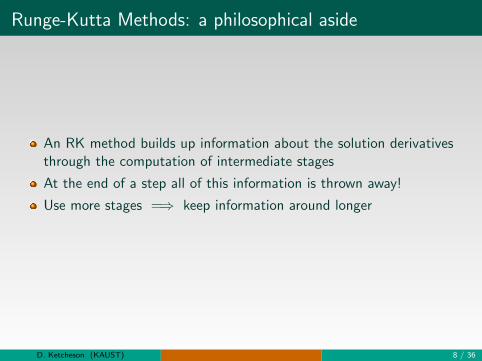
An RK method builds up information about the solution derivativesthrough the computation of intermediate stages
At the end of a step all of this information is thrown away!
Use more stages =⇒ keep information around longer
D. Ketcheson (KAUST) 8 / 36

Outline
1 High order Runge-Kutta methods
2 Linear properties of Runge-Kutta methods
3 Nonlinear properties of Runge-Kutta methods
4 Putting it all together: some optimal methods and applications
D. Ketcheson (KAUST) 9 / 36
The Stability Function
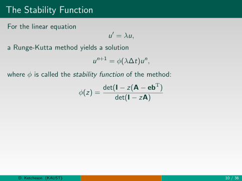
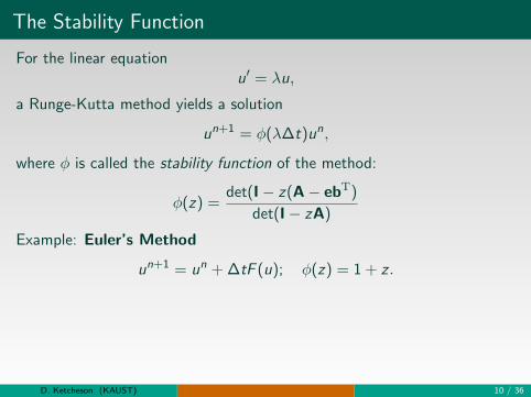
For the linear equationu′ = λu,
a Runge-Kutta method yields a solution
un+1 = φ(λ∆t)un,
where φ is called the stability function of the method:
φ(z) =det(I− z(A− ebT)
det(I− zA)
Example: Euler’s Method
un+1 = un + ∆tF (u); φ(z) = 1 + z .
For explicit methods of order p:
φ(z) =
p∑j=0
1
j!z j +
s∑j=p+1
αjzj .
D. Ketcheson (KAUST) 10 / 36
The Stability Function
For the linear equationu′ = λu,
a Runge-Kutta method yields a solution
un+1 = φ(λ∆t)un,
where φ is called the stability function of the method:
φ(z) =det(I− z(A− ebT)
det(I− zA)
Example: Euler’s Method
un+1 = un + ∆tF (u); φ(z) = 1 + z .
For explicit methods of order p:
φ(z) =
p∑j=0
1
j!z j +
s∑j=p+1
αjzj .
D. Ketcheson (KAUST) 10 / 36
Absolute Stability
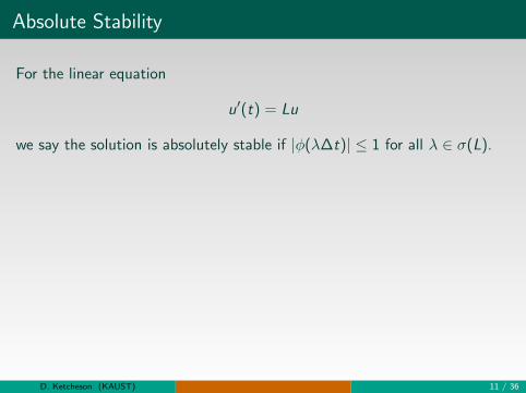
For the linear equation
u′(t) = Lu
we say the solution is absolutely stable if |φ(λ∆t)| ≤ 1 for all λ ∈ σ(L).
Example: Euler’s Method
un+1 = un + ∆tF (u); φ(z) = 1 + z .
−1
D. Ketcheson (KAUST) 11 / 36
Absolute Stability
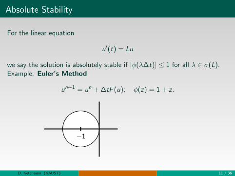
For the linear equation
u′(t) = Lu
we say the solution is absolutely stable if |φ(λ∆t)| ≤ 1 for all λ ∈ σ(L).Example: Euler’s Method
un+1 = un + ∆tF (u); φ(z) = 1 + z .
−1
D. Ketcheson (KAUST) 11 / 36
Stability optimization
This leads naturally to the following problem.
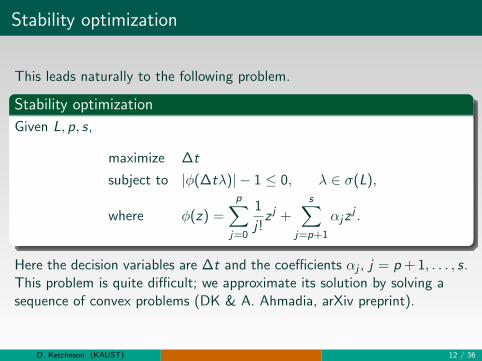
Stability optimization
Given L, p, s,
maximize ∆t
subject to |φ(∆tλ)| − 1 ≤ 0, λ ∈ σ(L),
where φ(z) =
p∑j=0
1
j!z j +
s∑j=p+1
αjzj .
Here the decision variables are ∆t and the coefficients αj , j = p + 1, . . . , s.This problem is quite difficult; we approximate its solution by solving asequence of convex problems (DK & A. Ahmadia, arXiv preprint).
D. Ketcheson (KAUST) 12 / 36
Accuracy optimization
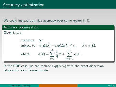
We could instead optimize accuracy over some region in C:
Accuracy optimization
Given L, p, s,
maximize ∆t
subject to |φ(∆tλ)− exp(∆tλ| ≤ ε, λ ∈ σ(L),
where φ(z) =
p∑j=0
1
j!z j +
s∑j=p+1
αjzj .
In the PDE case, we can replace exp(∆tλ) with the exact dispersionrelation for each Fourier mode.
D. Ketcheson (KAUST) 13 / 36

Stability Optimization: a toy example
As an example, consider the advection equation
ut + ux = 0
discretized in space by first-order upwind differencing with unit spatialmesh size
U ′i (t) = −(Ui (t)− Ui−1(t))
with periodic boundary condition U0(t) = UN(t).
4 3 2 10 18
6
4
2
0
2
4
6
8
D. Ketcheson (KAUST) 14 / 36
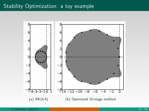
Stability Optimization: a toy example
4 3 2 10 18
6
4
2
0
2
4
6
8
(a) RK(4,4)
14 12 10 8 6 4 2 08
6
4
2
0
2
4
6
8
(b) Optimized 10-stage method
D. Ketcheson (KAUST) 15 / 36
Stability Optimization: a toy example
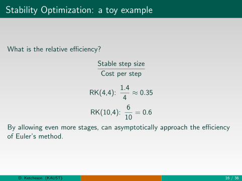
What is the relative efficiency?
Stable step size
Cost per step
RK(4,4):1.4
4≈ 0.35
RK(10,4):6
10= 0.6
By allowing even more stages, can asymptotically approach the efficiencyof Euler’s method.
D. Ketcheson (KAUST) 16 / 36
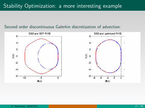
Stability Optimization: a more interesting example
Second order discontinuous Galerkin discretization of advection:
D. Ketcheson (KAUST) 17 / 36
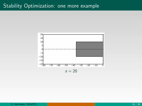
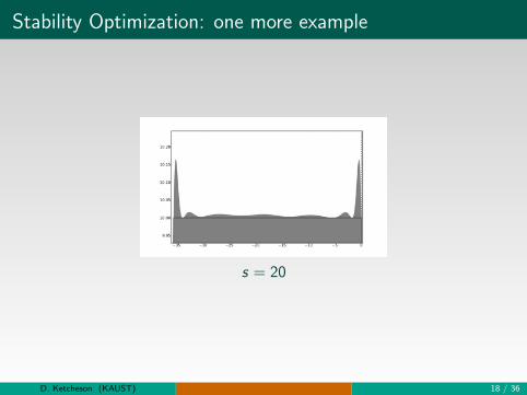
Stability Optimization: one more example
80 70 60 50 40 30 20 10 020
15
10
5
0
5
10
15
20
s = 20
D. Ketcheson (KAUST) 18 / 36
Stability Optimization: one more example
s = 20
D. Ketcheson (KAUST) 18 / 36

Stability Optimization: one more example
s = 20
D. Ketcheson (KAUST) 18 / 36

Outline
1 High order Runge-Kutta methods
2 Linear properties of Runge-Kutta methods
3 Nonlinear properties of Runge-Kutta methods
4 Putting it all together: some optimal methods and applications
D. Ketcheson (KAUST) 19 / 36
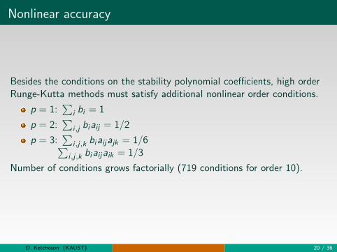
Nonlinear accuracy
Besides the conditions on the stability polynomial coefficients, high orderRunge-Kutta methods must satisfy additional nonlinear order conditions.
p = 1:∑
i bi = 1
p = 2:∑
i ,j biaij = 1/2
p = 3:∑
i ,j ,k biaijajk = 1/6∑i ,j ,k biaijaik = 1/3
Number of conditions grows factorially (719 conditions for order 10).
D. Ketcheson (KAUST) 20 / 36
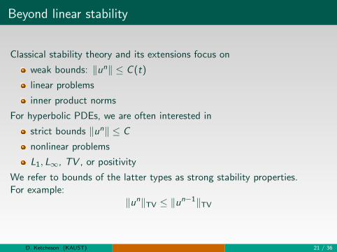
Beyond linear stability
Classical stability theory and its extensions focus on
weak bounds: ‖un‖ ≤ C (t)
linear problems
inner product norms
For hyperbolic PDEs, we are often interested in
strict bounds ‖un‖ ≤ C
nonlinear problems
L1, L∞, TV , or positivity
We refer to bounds of the latter types as strong stability properties.For example:
‖un‖TV ≤ ‖un−1‖TV
D. Ketcheson (KAUST) 21 / 36

Strong stability preservation
Designing fully-discrete schemes with strong stability properties isnotoriously difficult!
Instead, one often takes a method-of-lines approach and assumes explicitEuler time integration.
But in practice, we need to use higher order methods, for reasons of bothaccuracy and linear stability.Strong stability preserving methods provide higher order accuracy whilemaintaining any convex functional bound satisfied by Euler timestepping.
D. Ketcheson (KAUST) 22 / 36

Strong stability preservation
Designing fully-discrete schemes with strong stability properties isnotoriously difficult!Instead, one often takes a method-of-lines approach and assumes explicitEuler time integration.
But in practice, we need to use higher order methods, for reasons of bothaccuracy and linear stability.
Strong stability preserving methods provide higher order accuracy whilemaintaining any convex functional bound satisfied by Euler timestepping.
D. Ketcheson (KAUST) 22 / 36

Strong stability preservation
Designing fully-discrete schemes with strong stability properties isnotoriously difficult!Instead, one often takes a method-of-lines approach and assumes explicitEuler time integration.
But in practice, we need to use higher order methods, for reasons of bothaccuracy and linear stability.Strong stability preserving methods provide higher order accuracy whilemaintaining any convex functional bound satisfied by Euler timestepping.
D. Ketcheson (KAUST) 22 / 36
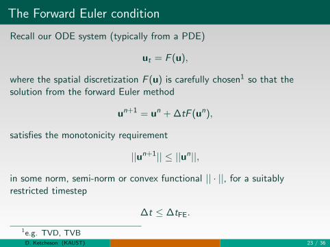
The Forward Euler condition
Recall our ODE system (typically from a PDE)
ut = F (u),
where the spatial discretization F (u) is carefully chosen1 so that thesolution from the forward Euler method
un+1 = un + ∆tF (un),
satisfies the monotonicity requirement
||un+1|| ≤ ||un||,
in some norm, semi-norm or convex functional || · ||, for a suitablyrestricted timestep
∆t ≤ ∆tFE.
1e.g. TVD, TVBD. Ketcheson (KAUST) 23 / 36
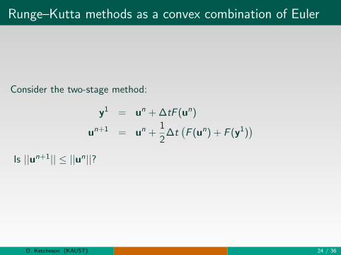
Runge–Kutta methods as a convex combination of Euler
Consider the two-stage method:
y1 = un + ∆tF (un)
un+1 = un +1
2∆t(F (un) + F (y1)
)Is ||un+1|| ≤ ||un||?
D. Ketcheson (KAUST) 24 / 36

Runge–Kutta methods as a convex combination of Euler
Consider the two-stage method:
y1 = un + ∆tF (un)
un+1 =1
2un +
1
2
(y1 + ∆tF (y1)
).
Take ∆t ≤ ∆tFE. Then ||y1|| ≤ ||un||, so
||un+1|| ≤ 1
2||un||+ 1
2||y1 + ∆tF (y1)|| ≤ ||un||.
||un+1|| ≤ ||un||
D. Ketcheson (KAUST) 24 / 36

Optimized SSP methods
In general, an SSP method preserves strong stability properties satisfied byEuler’s method, under a modified step size restriction:
∆t ≤ C∆tFE.
A fair metric for comparison is the effective SSP coefficient:
Ceff =C
# of stages
By designing high order methods with many stages, we can achieveCeff → 1.
D. Ketcheson (KAUST) 25 / 36
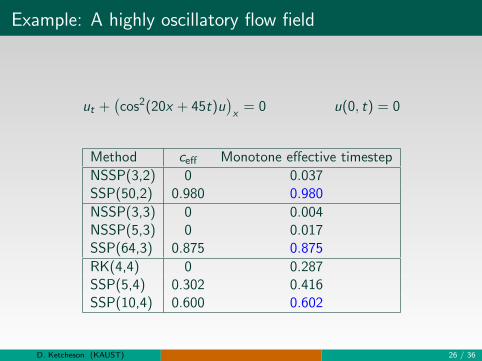
Example: A highly oscillatory flow field
ut +(cos2(20x + 45t)u
)x
= 0 u(0, t) = 0
Method ceff Monotone effective timestep
NSSP(3,2) 0 0.037SSP(50,2) 0.980 0.980
NSSP(3,3) 0 0.004NSSP(5,3) 0 0.017SSP(64,3) 0.875 0.875
RK(4,4) 0 0.287SSP(5,4) 0.302 0.416SSP(10,4) 0.600 0.602
D. Ketcheson (KAUST) 26 / 36
Low storage methods
Straightforward implementation of an s-stage RK method requiress + 1 memory locations per unknown
Special low-storage methods are designed so that each stage onlydepends on one or two most recent previous stages
Thus older stages can be discarded as the new ones are computed
It is often desirable to
Keep the previous solution around to be able to restart a stepCompute an error estimate
This requires a minimum of three storage locations per unknown
D. Ketcheson (KAUST) 27 / 36
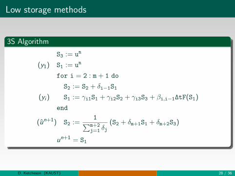
Low storage methods
3S Algorithm
S3 := un
(y1) S1 := un
for i = 2 : m + 1 do
S2 := S2 + δi−1S1
(yi ) S1 := γi1S1 + γi2S2 + γi3S3 + βi,i−1∆tF(S1)
end
(un+1) S2 :=1∑m+2
j=1 δj(S2 + δm+1S1 + δm+2S3)
un+1 = S1
D. Ketcheson (KAUST) 28 / 36

Outline
1 High order Runge-Kutta methods
2 Linear properties of Runge-Kutta methods
3 Nonlinear properties of Runge-Kutta methods
4 Putting it all together: some optimal methods and applications
D. Ketcheson (KAUST) 29 / 36
Two-step optimization process
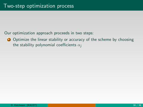
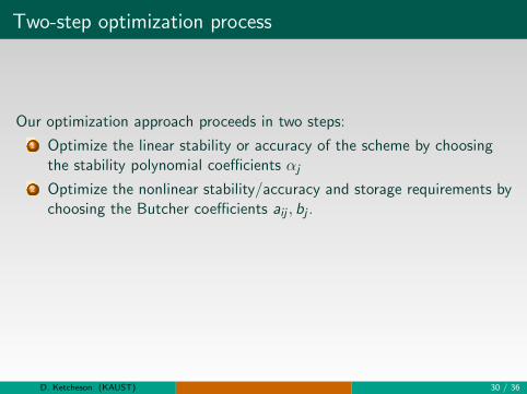
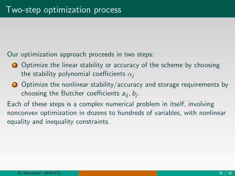
Our optimization approach proceeds in two steps:
1 Optimize the linear stability or accuracy of the scheme by choosingthe stability polynomial coefficients αj
2 Optimize the nonlinear stability/accuracy and storage requirements bychoosing the Butcher coefficients aij , bj .
Each of these steps is a complex numerical problem in itself, involvingnonconvex optimization in dozens to hundreds of variables, with nonlinearequality and inequality constraints.
D. Ketcheson (KAUST) 30 / 36
Two-step optimization process
Our optimization approach proceeds in two steps:
1 Optimize the linear stability or accuracy of the scheme by choosingthe stability polynomial coefficients αj
2 Optimize the nonlinear stability/accuracy and storage requirements bychoosing the Butcher coefficients aij , bj .
Each of these steps is a complex numerical problem in itself, involvingnonconvex optimization in dozens to hundreds of variables, with nonlinearequality and inequality constraints.
D. Ketcheson (KAUST) 30 / 36

Optimizing for the SD spectrum
On regular grids, SD leads to a block-Toeplitz operator
We perform a von Neumann-like analysis using a ”generating pattern”
i + 1, j ! 1
i + 1, ji ! 1, j
!g2
!g1
i, j + 1 i + 1, j + 1
i, j
i ! 1, j + 1
i ! 1, j ! 1 i, j ! 1
dWi ,j
dt+
a
∆g
(T0,0 Wi ,j + T−1,0 Wi−1,j + T0,−1 Wi ,j−1
+T+1,0 Wi+1,j + T0,+1 Wi ,j+1
)= 0
D. Ketcheson (KAUST) 31 / 36

Optimizing for the SD spectrum
Blue: eigenvalues; Red: RK stability boundary
The convex hull of the generated spectrum is used as a proxy toaccelerate the optimization process
D. Ketcheson (KAUST) 32 / 36
Optimizing for the SD spectrum
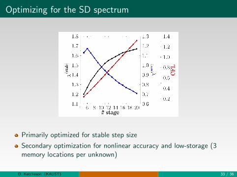
Primarily optimized for stable step size
Secondary optimization for nonlinear accuracy and low-storage (3memory locations per unknown)
D. Ketcheson (KAUST) 33 / 36
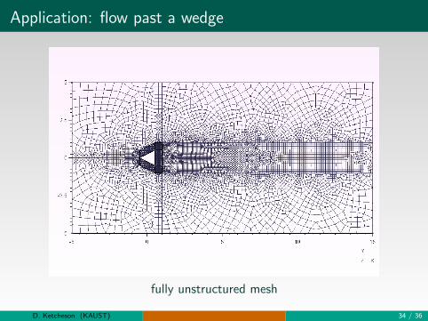
Application: flow past a wedge
fully unstructured mesh
D. Ketcheson (KAUST) 34 / 36

Application: flow past a wedge
Density at t = 100
62% speedup using optimized method
D. Ketcheson (KAUST) 35 / 36

Conclusions
Numerical optimization allows for flexible, targeted design of timeintegrators
Stability optimization based on spectra from a model (linear) problemon a uniform grid seems to work well even for nonlinear problems onfully unstructured grids
Significant speedup can be achieved in practice (greater for higherorder methods)
D. Ketcheson (KAUST) 36 / 36

![RUNGE-KUTTA METHODS FOR PARABOLIC …...ity properties with high order1 (cf. the discussion of Runge-Kutta vs. multistep methods in the stiff ODE case [9]). In 3 we study Runge-Kutta](https://img.pdfslide.net/doc/110x75/5e5ec0fd3371f85b7a4d4f58/runge-kutta-methods-for-parabolic-ity-properties-with-high-order1-cf-the-discussion.jpg)