Design of Parallel and High-PerformanceComputingFall 2017Lecture: distributed memory

Instructor: Torsten Hoefler & Markus Püschel

TA: Salvatore Di Girolamo

Motivational video: https://www.youtube.com/watch?v=PuCx50FdSic

Administrivia

Final project presentation: Monday 12/18 (next week)

Should have (pretty much) final results

Show us how great your project is

Some more ideas what to talk about:

Which architecture(s) did you test on?

How did you verify correctness of the parallelization?

Use bounds models for comparisons [1]!

(Somewhat) realistic use-cases and input sets?

Emphasize on the key concepts (may relate to theory of lecture)!

What are remaining issues/limitations?

Report will be due in January!

Still, starting to write early is very helpful --- write – rewrite – rewrite (no joke!)

2[1]: T. Hoefler, R. Belli: Scientific Benchmarking of Parallel Computing Systems, IEEE/ACM SC15

Review of last lecture

Practical lock properties

RW locks

Lock properties/issues (deadlock, priority inversion, blocking vs. spinning)

Competitive spinning

Locked and lock-free tricks

Fine-grained locking

RW locking

Optimistic synchronization

Lazy locking

Lock-free (& wait-free)

3

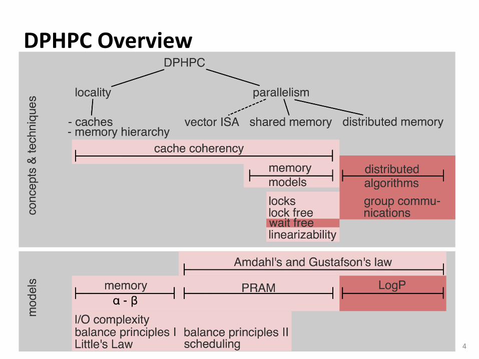
DPHPC Overview

4

Goals of this lecture Finish wait-free/lock-free

Consensus hierarchy

The promised proof!

Some glimpse of distributed memory

High-performance computing

Research topics

Parallel and distributed machine learning

5

Comments on the parallel patterns tricks

Correctness proof techniques

Establish invariants for initial state and transformations

E.g., head and tail are never removed, every node in the set has to be reachable from head, …

Proofs are similar to those we discussed for locks

Very much the same techniques (just trickier)

Using sequential consistency (or consistency model of your choice )

Lock-free gets somewhat tricky

Source-codes can be found in Chapter 9 of “The Art of Multiprocessor Programming”

6

Defining lock-free and wait-free

A lock-free method

guarantees that infinitely often some method call finishes in a finite number of steps

A wait-free method

guarantees that each method call finishes in a finite number of steps (implies lock-free)

Synchronization instructions are not equally powerful!

Indeed, they form an infinite hierarchy; no instruction (primitive) in level x can be used for lock-/wait-free implementations of primitives in level z>x.

7

Concept: Consensus Number

Each level of the hierarchy has a “consensus number” assigned.

Is the maximum number of threads for which primitives in level x can solve the consensus problem

The consensus problem:

Has single function: decide(v)

Each thread calls it at most once, the function returns a value that meets two conditions:

consistency: all threads get the same value

validity: the value is some thread’s input

Simplification: binary consensus (inputs in {0,1})

8

Understanding Consensus

Can a particular class solve n-thread consensus wait-free?

A class C solves n-thread consensus if there exists a consensus protocol using any number of objects of class C and any number of atomic registers

The protocol has to be wait-free (bounded number of steps per thread)

The consensus number of a class C is the largest n for which that class solves n-thread consensus (may be infinite)

Class question:

Assume we have a class D whose objects can be constructed from objects out of class C. If class C has consensus number n, what does class D have?

9

Starting simple …

Binary consensus with two threads (A, B)!

Each thread moves until it decides on a value

May update shared objects

Protocol state = state of threads + state of shared objects

Initial state = state before any thread moved

Final state = state after all threads finished

States form a tree, wait-free property guarantees a finite tree

Example with two threads and two moves each!

10

Atomic Registers

Theorem [Herlihy’91]: Atomic registers have consensus number one

I.e., they cannot be used to solve even two-thread consensus! Really?

Proof outline:

Assume arbitrary consensus protocol, thread A, B

Run until it reaches critical state where next action determines outcome (show that it must have a critical state first)

Show all options using atomic registers and show that they cannot be used to determine one outcome for all possible executions!

1) Any thread reads (other thread runs solo until end)

2) Threads write to different registers (order doesn’t matter)

3) Threads write to same register (solo thread can start after each write)

11

Atomic Registers

Theorem [Herlihy’91]: Atomic registers have consensus number one

Corollary: It is impossible to construct a wait-free implementation of any object with consensus number of >1 using atomic registers “perhaps one of the most striking impossibility results in Computer

Science” (Herlihy, Shavit) We need hardware atomics or Transactional Memory!

Proof technique borrowed from:

Very influential paper, always worth a read! Nicely shows proof techniques that are central to parallel and distributed

computing!

12

Other Atomic Operations

Simple RMW operations (Test&Set, Fetch&Op, Swap, basically all functions where the op commutes or overwrites) have consensus number 2!

Similar proof technique (bivalence argument)

CAS and TM have consensus number ∞

Constructive proof!

13

Compare and Set/Swap Consensus

CAS provides an infinite consensus number

Machines providing CAS are asynchronous computation equivalents of the Turing Machine

I.e., any concurrent object can be implemented in a wait-free manner (not necessarily fast!)

14

const int first = -1volatile int thread = -1;int proposed[n];

int decide(v) {proposed[tid] = v;if(CAS(thread, first, tid))

return v; // I won!else

return proposed[thread]; // thread won}

Now you know everything

Not really … ;-)

We’ll argue more about performance now!

But you have all the tools for:

Efficient locks

Efficient lock-based algorithms

Efficient lock-free algorithms (or even wait-free)

Reasoning about parallelism!

What now?

A different class of problems

Impact on wait-free/lock-free on actual performance is not well understood

Relevant to HPC, applies to shared and distributed memory

Group communications

15

Remember: A Simple Model for Communication

Transfer time T(s) = α+βs

α = startup time (latency)

β = cost per byte (bandwidth=1/β)

As s increases, bandwidth approaches 1/β asymptotically

Convergence rate depends on α

s1/2 = α/β

Assuming no pipelining (new messages can only be issued from a process after all arrived)

16

Bandwidth vs. Latency

s1/2 = α/β often used to distinguish bandwidth- and latency-

bound messages

s1/2 is in the order of kilobytes on real systems

17

asymptotic limitfor β=2

Quick Example

Simplest linear broadcast

One process has a data item to be distributed to all processes

Broadcasting s bytes among P processes:

T(s) = (P-1) * (α+βs) =

Class question: Do you know a faster method to accomplish the same?

18

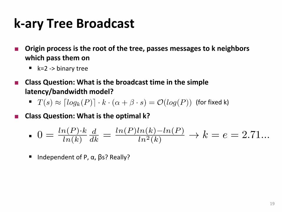
k-ary Tree Broadcast

Origin process is the root of the tree, passes messages to k neighbors which pass them on

k=2 -> binary tree

Class Question: What is the broadcast time in the simple latency/bandwidth model?

(for fixed k)

Class Question: What is the optimal k?

Independent of P, α, βs? Really?

19

Faster Trees?

Class Question: Can we broadcast faster than in a ternary tree?

Yes because each respective root is idle after sending three messages!

Those roots could keep sending!

Result is a k-nomial tree

For k=2, it’s a binomial tree

Class Question: What about the runtime?

Class Question: What is the optimal k here?

T(s) d/dk is monotonically increasing for k>1, thus kopt=2

Class Question: Can we broadcast faster than in a k-nomial tree?

is asymptotically optimal for s=1!

But what about large s?

20

Open Problems

Look for optimal parallel algorithms (even in simple models!)

And then check the more realistic models

Useful optimization targets are MPI collective operations

Broadcast/Reduce, Scatter/Gather, Alltoall, Allreduce, Allgather, Scan/Exscan, …

Implementations of those (check current MPI libraries )

Useful also in scientific computations

Barnes Hut, linear algebra, FFT, …

Lots of work to do!

Contact me for thesis ideas (or check SPCL) if you like this topic

Usually involve optimization (ILP/LP) and clever algorithms (algebra) combined with practical experiments on large-scale machines (10,000+ processors)

24

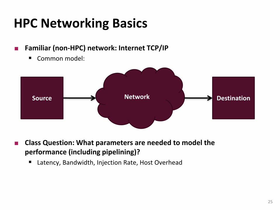
HPC Networking Basics

Familiar (non-HPC) network: Internet TCP/IP

Common model:

Class Question: What parameters are needed to model the performance (including pipelining)?

Latency, Bandwidth, Injection Rate, Host Overhead

25

Network DestinationSource

The LogP Model

Defined by four parameters:

L: an upper bound on the latency, or delay, incurred in communicating a message containing a word (or small number of words) from its source module to its target module.

o: the overhead, defined as the length of time that a processor is engaged in the transmission or reception of each message; during this time, the processor cannot perform other operations.

g: the gap, defined as the minimum time interval between consecutive message transmissions or consecutive message receptions at a processor. The reciprocal of g corresponds to the available per-processor communication bandwidth.

P: the number of processor/memory modules. We assume unit time for local operations and call it a cycle.

26

The LogP Model

27

Simple Examples

Sending a single message

T = 2o+L

Ping-Pong Round-Trip

TRTT = 4o+2L

Transmitting n messages

T(n) = L+(n-1)*max(g, o) + 2o

28

Simplifications

o is bigger than g on some machines

g can be ignored (eliminates max() terms)

be careful with multicore!

Offloading networks might have very low o

Can be ignored (not yet but hopefully soon)

L might be ignored for long message streams

If they are pipelined

Account g also for the first message

Eliminates “-1”

29

Benefits over Latency/Bandwidth Model

Models pipelining

L/g messages can be “in flight”

Captures state of the art (cf. TCP windows)

Models computation/communication overlap

Asynchronous algorithms

Models endpoint congestion/overload

Benefits balanced algorithms

30

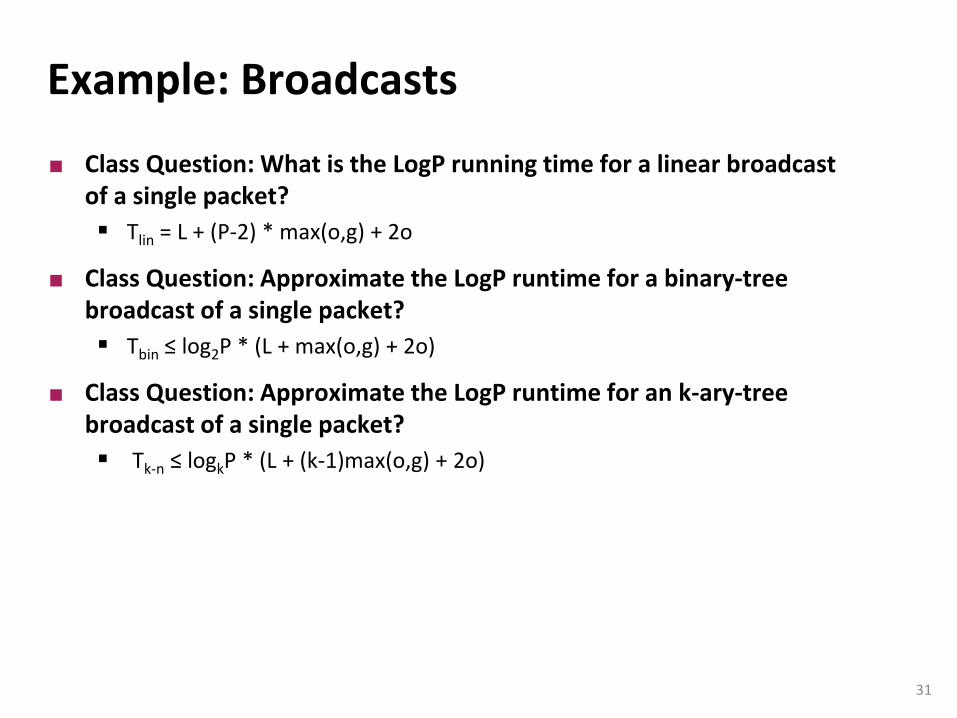
Example: Broadcasts

Class Question: What is the LogP running time for a linear broadcast of a single packet?

Tlin = L + (P-2) * max(o,g) + 2o

Class Question: Approximate the LogP runtime for a binary-tree broadcast of a single packet?

Tbin ≤ log2P * (L + max(o,g) + 2o)

Class Question: Approximate the LogP runtime for an k-ary-tree broadcast of a single packet?

Tk-n ≤ logkP * (L + (k-1)max(o,g) + 2o)

31

Example: Broadcasts

Class Question: Approximate the LogP runtime for a binomial tree broadcast of a single packet (assume L > g!)?

Tbin ≤ log2P * (L + 2o)

Class Question: Approximate the LogP runtime for a k-nomial tree broadcast of a single packet?

Tk-n ≤ logkP * (L + (k-2)max(o,g) + 2o)

Class Question: What is the optimal k (assume o>g)?

Derive by k: 0 = o * ln(kopt) – L/kopt + o (solve numerically)

For larger L, k grows and for larger o, k shrinks

Models pipelining capability better than simple model!

32

Example: Broadcasts

Class Question: Can we do better than kopt-ary binomial broadcast?

Problem: fixed k in all stages might not be optimal

We can construct a schedule for the optimal broadcast in practical settings

First proposed by Karp et al. in “Optimal Broadcast and Summation in the LogP Model”

33

Example: Optimal Broadcast

Broadcast to P-1 processes

Each process who received the value sends it on; each process receives exactly once

34

P=8, L=6, g=4, o=2

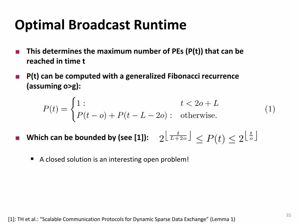
Optimal Broadcast Runtime

This determines the maximum number of PEs (P(t)) that can be reached in time t

P(t) can be computed with a generalized Fibonacci recurrence (assuming o>g):

Which can be bounded by (see [1]):

A closed solution is an interesting open problem!

35[1]: TH et al.: “Scalable Communication Protocols for Dynamic Sparse Data Exchange” (Lemma 1)

The Bigger Picture

We learned how to program shared memory systems

Coherency & memory models & linearizability

Locks as examples for reasoning about correctness and performance

List-based sets as examples for lock-free and wait-free algorithms

Consensus number

We learned about general performance properties and parallelism

Amdahl’s and Gustafson’s laws

Little’s law, Work-span, …

Balance principles & scheduling

We learned how to perform model-based optimizations

Distributed memory broadcast example with two models

What next? MPI? OpenMP? UPC?

Next-generation machines “merge” shared and distributed memory concepts → Partitioned Global Address Space (PGAS)

36