1

Design of Robust Higher Order Sliding ModeControl for Microgrids

Michele Cucuzzella, Gian Paolo Incremona, and Antonella Ferrara

Abstract—This paper deals with the design of advanced controlstrategies of sliding mode type for microgrids. Each distributedgeneration unit (DGu), constituting the considered microgrid,can work in both grid-connected operation mode (GCOM) andislanded operation mode (IOM). The DGu is affected by loadvariations, nonlinearities and unavoidable modelling uncertain-ties. This makes sliding mode control particularly suitable as asolution methodology for the considered problem. In particular, asecond order sliding mode (SOSM) control algorithm, belongingto the class of Suboptimal SOSM control, is proposed for bothGCOM and IOM, while a third-order sliding mode (3-SM)algorithm is designed only for IOM, in order to achieve, alsoin this case, satisfactory chattering alleviation. The microgridsystem controlled via the proposed sliding mode control lawsexhibits appreciable stability properties, which are formallyanalyzed in the paper. Simulation results also confirm thatthe obtained closed-loop performances comply with the IEEErecommendations for power systems.

Index Terms—Sliding modes, power systems, uncertain sys-tems.

I. INTRODUCTION

In recent years, the increasing of renewable energy sourceshas given rise to a new paradigm in power generation. There isa clear trend towards the realization of smaller DGus [1], whichenables to achieve economical and environmental benefits, interms of energy efficiency and reduced carbon emissions [2].DGus also improve the service continuity [3], by supplyinga portion of the load, even after being disconnected from themain grid [4].

In the literature, a set of interconnected DGus, which areusually strictly close to the energy consumers, is identified as a“microgrid” [5]–[7]. The latter, characterized by some intelligentcomputation and metering capability, can be considered as thebasic unit of the so-called “smart grid" [8]. Because of theintermittence and the uncertainty caused by meteorologicalfactors, it is difficult to integrate renewable energy sourcesdirectly into the main grid. This is the reason why voltagecontrol, power control, fault detection, reliability enforcement,and power losses minimization are among the issues to solve inorder to integrate DGus into the distribution network [9], [10].In recent years, several control strategies have been proposedto deal with DGus. Many of them are based on PI controllers

This is the final version of the accepted paper submitted to IEEE Journalon Emerging and Selected Topics in Circuits and Systems. Copyright (c)2015 IEEE. Personal use of this material is permitted. However, permissionto use this material for any other purposes must be obtained from theIEEE by sending an email to pubs-permissions@ieee.org. M.Cucuzzella, G. P. Incremona and A. Ferrara are with the Dipartimento diIngegneria Industriale e dell’Informazione, University of Pavia, via Ferrata1, 27100 Pavia, Italy (e-mail: michele.cucuzzella@gmail.com,gp.incremona@gmail.com, a.ferrara@unipv.it).

and consider the microgrid in IOM (see [11]–[15]). Othersadopt more advanced control methodologies such as droopmode control [16], [17], predictive control [18], [19], adaptivecontrol [20], [21], H∞ control [22], and Plug-and-Play (PnP)decentralized algorithms [23].

One of the crucial problems in microgrids is the presence ofthe voltage-sourced-converter (VSC) as interface element withthe main grid. The VSC can be viewed as a source of modellinguncertainty and disturbances. This fact makes the adoption ofa robust control design methodology mandatory. Sliding mode(SM) control [24], [25] is a well-known control approach partic-ularly appreciated for its robustness properties. Specifically, it isable to reject the so-called matched uncertainties, i.e., unknownterms which act on the same channel of the control variable,and not to amplify unmatched disturbances [26]. SM controlis easy to implement, yet, it requires the use of discontinuouscontrol laws, which can enforce the chattering effect, i.e., highfrequency oscillations of the controlled variable due to thediscontinuities of the control law, [27]–[29]. In the literature,several methods to alleviate chattering, such as boundary layercontrol or filtered control, have been proposed. Yet, in thesecases the robustness properties typical of SM control couldbe lost. An effective way to perform chattering alleviation isinstead to increase the order of the sliding mode. For thisreason Higher Order Sliding Mode (HOSM) control laws [30],in particular of the second order, have been studied.

In this paper, a master-slave scheme with advanced controlstrategies, which belong to the class of Suboptimal SOSMalgorithms [31]–[34] and of min−max Time-optimal third-order SM (3-SM) algorithms [30], is proposed. First, the useof SOSM control is investigated, observing how this approachcan provide satisfactory chattering alleviation only in case ofGCOM, since in that case the controlled system relative degreeis unitary, while in IOM it is equal to 2. Then, to attain achattering attenuation effect also in IOM, a 3-SM control lawis designed for that case. So, on the whole, it is possible todevise a control policy which switches from a SOSM controllaw to a 3-SM control law, i.e., changes the order of the slidingmodes which are generated, whenever a transition from GCOMto IOM occurs.

Note that, preliminary and partial versions of this work, notreporting the proofs of stability and robustness, have beenpublished in [35], [36].

II. PRELIMINARY ISSUES

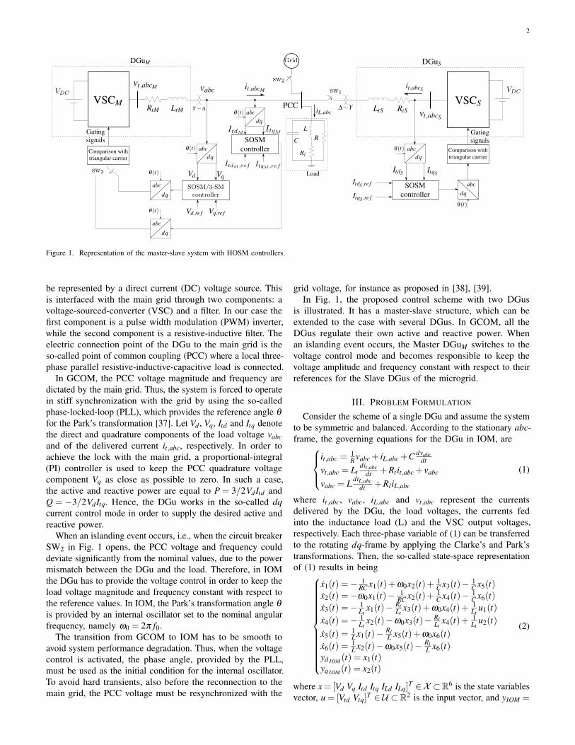
Consider the schematic electric single-line diagram of twointerconnected DGus in Fig. 1. The basic element of a DGuis usually an energy source of renewable type, which can

2

Figure 1. Representation of the master-slave system with HOSM controllers.

be represented by a direct current (DC) voltage source. Thisis interfaced with the main grid through two components: avoltage-sourced-converter (VSC) and a filter. In our case thefirst component is a pulse width modulation (PWM) inverter,while the second component is a resistive-inductive filter. Theelectric connection point of the DGu to the main grid is theso-called point of common coupling (PCC) where a local three-phase parallel resistive-inductive-capacitive load is connected.

In GCOM, the PCC voltage magnitude and frequency aredictated by the main grid. Thus, the system is forced to operatein stiff synchronization with the grid by using the so-calledphase-locked-loop (PLL), which provides the reference angle θ

for the Park’s transformation [37]. Let Vd , Vq, Itd and Itq denotethe direct and quadrature components of the load voltage vabcand of the delivered current it,abc, respectively. In order toachieve the lock with the main grid, a proportional-integral(PI) controller is used to keep the PCC quadrature voltagecomponent Vq as close as possible to zero. In such a case,the active and reactive power are equal to P = 3/2VdItd andQ = −3/2VdItq. Hence, the DGu works in the so-called dqcurrent control mode in order to supply the desired active andreactive power.

When an islanding event occurs, i.e., when the circuit breakerSW2 in Fig. 1 opens, the PCC voltage and frequency coulddeviate significantly from the nominal values, due to the powermismatch between the DGu and the load. Therefore, in IOMthe DGu has to provide the voltage control in order to keep theload voltage magnitude and frequency constant with respect tothe reference values. In IOM, the Park’s transformation angle θ

is provided by an internal oscillator set to the nominal angularfrequency, namely ω0 = 2π f0.

The transition from GCOM to IOM has to be smooth toavoid system performance degradation. Thus, when the voltagecontrol is activated, the phase angle, provided by the PLL,must be used as the initial condition for the internal oscillator.To avoid hard transients, also before the reconnection to themain grid, the PCC voltage must be resynchronized with the

grid voltage, for instance as proposed in [38], [39].In Fig. 1, the proposed control scheme with two DGus

is illustrated. It has a master-slave structure, which can beextended to the case with several DGus. In GCOM, all theDGus regulate their own active and reactive power. Whenan islanding event occurs, the Master DGuM switches to thevoltage control mode and becomes responsible to keep thevoltage amplitude and frequency constant with respect to theirreferences for the Slave DGus of the microgrid.

III. PROBLEM FORMULATION

Consider the scheme of a single DGu and assume the systemto be symmetric and balanced. According to the stationary abc-frame, the governing equations for the DGu in IOM, are

it,abc =1R vabc + iL,abc +C dvabc

dt

vt,abc = Ltdit,abc

dt +Rt it,abc + vabc

vabc = L diL,abcdt +Rl iL,abc

(1)

where it,abc, vabc, iL,abc and vt,abc represent the currentsdelivered by the DGu, the load voltages, the currents fedinto the inductance load (L) and the VSC output voltages,respectively. Each three-phase variable of (1) can be transferredto the rotating dq-frame by applying the Clarke’s and Park’stransformations. Then, the so-called state-space representationof (1) results in being

x1(t) =− 1RC x1(t)+ω0x2(t)+ 1

C x3(t)− 1C x5(t)

x2(t) =−ω0x1(t)− 1RC x2(t)+ 1

C x4(t)− 1C x6(t)

x3(t) =− 1Lt

x1(t)− RtLt

x3(t)+ω0x4(t)+ 1Lt

u1(t)x4(t) =− 1

Ltx2(t)−ω0x3(t)− Rt

Ltx4(t)+ 1

Ltu2(t)

x5(t) = 1L x1(t)− Rl

L x5(t)+ω0x6(t)x6(t) = 1

L x2(t)−ω0x5(t)− RlL x6(t)

yd IOM (t) = x1(t)yq IOM (t) = x2(t)

(2)

where x= [Vd Vq Itd Itq ILd ILq]T ∈X ⊂R6 is the state variables

vector, u = [Vtd Vtq]T ∈ U ⊂R2 is the input vector, and yIOM =

3

[Vd Vq]T ∈R2 is the output vector. Analogously, the state-space

model of the DGu in GCOM is

x1(t) =− 1RC x1(t)+ωx2(t)+ 1

C x3(t)− 1C x5(t)− 1

C x7(t)x2(t) =−ωx1(t)− 1

RC x2(t)+ 1C x4(t)− 1

C x6(t)− 1C x8(t)

x3(t) =− 1Lt

x1(t)− RtLt

x3(t)+ωx4(t)+ 1Lt

u1(t)x4(t) =− 1

Ltx2(t)−ωx3(t)− Rt

Ltx4(t)+ 1

Ltu2(t)

x5(t) = 1L x1(t)− Rl

L x5(t)+ωx6(t)x6(t) = 1

L x2(t)−ωx5(t)− RlL x6(t)

x7(t) = 1Ls

x1(t)− RsLs

x7(t)+ωx8(t)− 1Ls

u3(t)x8(t) = 1

Lsx2(t)−ωx7(t)− Rs

Lsx8(t)− 1

Lsu4(t)

yd GCOM (t) = x3(t)yqGCOM (t) = x4(t)

(3)

where x = [Vd Vq Itd Itq ILd ILq Igd Igq]T ∈ X ⊂R8 is the state

variables vector, u = [Vtd Vtq Vgd Vgq]T ∈ U ⊂ R4 is the input

vector, and yGCOM = [Itd Itq]T ∈R2 is the output vector, Igd , Igq,Vgd , Vgq being the dq-components of the currents exchangedwith the grid and the grid voltages.

The aim of this paper consists in designing a control schemecapable of guaranteeing that the tracking error between anycontrolled variable and the corresponding reference is steeredto zero in a finite time in spite of the uncertainties.

IV. THE PROPOSED SOLUTION: HIGHER ORDER SLIDINGMODE CONTROL SCHEME

In this section, the use of HOSM control to solve theaforementioned control problem is discussed.

A. Suboptimal SOSM ControllerConsider the IOM state-space model (2) and select the so-

called “sliding variables” as

σdIOM (t) = ydIOM ,re f − ydIOM (t) (4)σqIOM (t) = yqIOM ,re f − yqIOM (t) (5)

where yiIOM ,re f , i = d,q are assumed to be of class C2 and withsecond time derivative Lipschitz continuous. Denote with rthe relative degree of the system, i.e., the minimum order rof the time derivative σ (r) of the sliding variable in whichthe control u explicitly appears. With reference to (4)-(5), itappears that r is equal to 2. This implies that a SOSM controlnaturally applies [31], [32]. According to the SOSM controltheory, we need to define the so-called auxiliary variablesξd,1IOM =σdIOM and ξq,1IOM =σqIOM such that the correspondingauxiliary systems can be expressed as

ξi,1IOM (t) = ξi,2IOM (t)ξi,2IOM (t) = fiIOM (x(t))+giIOM uiIOM (t)

i = d,q (6)

where uiIOM are the dq-components of the VSC output voltages,ξi,2IOM are assumed to be unmeasurable, and

fdIOM (x(t)) = (ω20 −

1(RC)2 +

1LtC + 1

LC )x1(t)+2ω0RC x2(t)

+( 1RC2 +

RtLtC )x3(t)− 2ω0

C x4(t)−( 1

RC2 +RlLC )x5(t)+

2ω0C x6(t)+ x1,re f (t)

fqIOM (x(t)) =− 2ω0RC x1(t)+(ω2

0 −1

(RC)2 +1

LtC + 1LC )x2(t)

+ 2ω0C x3(t)+( 1

RC2 +Rt

LtC )x4(t)− 2ω0

C x5(t)− ( 1RC2 +

RlLC )x6(t)+ x2,re f (t)

giIOM =− 1LtC , i = d,q

(7)

are allowed to be uncertain with known bounds

| fiIOM (·)| ≤ FiIOM , Gi,mIOM ≤ |giIOM | ≤ Gi,MIOM (8)

FiIOM , Gi,mIOM and Gi,MIOM being positive constants. Note that,the existence of these bounds is true in practice due to thefact that fiIOM (·), i = d,q, depend on electric signals related tothe finite power of the system and giIOM , i = d,q, are constantvalues. The control laws, which are proposed to steer ξi,1IOM (t)and ξi,2IOM (t), i = d,q, to zero in a finite time in spite of theuncertainties, in analogy with [31], can be expressed as follows

uiIOM (t) =−αiIOMUiIOM,max sgn(

ξi,1IOM (t)−12 ξi,1IOM,max

)(9)

with bounds

UiIOM,max > max

(FiIOM

α∗iIOMGi,mIOM

;4FiIOM

3Gi,mIOM −α∗iIOMGi,MIOM

)(10)

α∗iIOM∈ (0,1]∩

(0,

3Gi,mIOM

Gi,MIOM

)(11)

Analogously, in GCOM, the sliding variables are selected as

σdGCOM (t) = ydGCOM ,re f − ydGCOM (t) (12)σqGCOM (t) = yqGCOM ,re f − yqGCOM (t) (13)

where yiGCOM ,re f , i = d,q are assumed to be of class C andwith first time derivative Lipschitz continuous. In this secondcase, the natural relative degree of the system is equal to 1.So, a first order sliding mode controller would be adequate.Yet, in order to alleviate the chattering phenomenon [27]–[29],[40], [41], which can be dangerous in terms of harmonicsaffecting the electric signals, SOSM control is used also in thiscase, by artificially increasing the relative degree of the system.Specifically, by defining the auxiliary variables ξd,1GCOM =σdGCOM and ξq,1GCOM = σqGCOM , one hasξi,1GCOM (t) = ξi,2GCOM (t)

ξi,2GCOM (t) = fiGCOM (x(t),u(t))+giGCOM wiGCOM (t)uiGCOM (t) = wiGCOM (t)

i = d,q

(14)

where uiGCOM , are the dq-components of the VSC outputvoltages, ξi,2GCOM are assumed to be unmeasurable, and

fdGCOM (x(t),u(t)) =−( 1RLtC + Rt

L2t)x1(t)+ 2ω

Ltx2(t)

+(ω2 + 1LtC −

R2t

L2t)x3(t)+

2ωRtLt

x4(t)

− 1LtC x5(t)− 1

LtC x7(t)+RtL2

tudGCOM (t)

− ω

LtuqGCOM (t)+ x3,re f (t)

fqGCOM (x(t),u(t)) =− 2ω

Ltx1(t)− ( 1

RLtC + RtL2

t)x2(t)

− 2ωRtLt

x3(t)+(ω2 + 1LtC −

R2t

L2t)x4(t)

− 1LtC x6(t)− 1

LtC x8(t)+ ω

LtudGCOM (t)

+ RtL2

tuqGCOM (t)+ x4,re f (t)

giGCOM =− 1Lt, i = d,q

(15)

are allowed to be uncertain with known bounds

| fiGCOM (·)| ≤ FiGCOM , Gi,mGCOM ≤ |giGCOM | ≤Gi,MGCOM (16)

FiGCOM , Gi,mGCOM and Gi,MGCOM being positive constants. The

4

control laws, which are proposed to steer ξi,1GCOM (t) andξi,2GCOM (t), i = d,q, to zero in a finite time in spite of theuncertainties, in this second case, can be expressed as follows

wiGCOM =−αiGCOMUiGCOM,max sgn(

ξi,1GCOM −12 ξi,1GCOM,max

)(17)

with bounds

UiGCOM,max > max

(FiGCOM

α∗iGCOMGi,mGCOM

;4FiGCOM

3Gi,mGCOM −α∗iGCOMGi,MGCOM

)(18)

α∗iGCOM

∈ (0,1]∩(

0,3Gi,mGCOM

Gi,MGCOM

)(19)

Note that, the discontinuity of the SOSM control laws wiGCOM ,i = d,q only affects σiGCOM . The actual control variables uiGCOM ,i = d,q, are continuous, so that the chattering is alleviated.

Moreover, in order to face some undesired overshoot on thecurrents, due to the reconnection to the main grid, as well asstep variations of the current references, a constrained SOSM(SOSMc) can be used in GCOM. According to [42], this isable to fulfil the constraints imposed on ξi,1GCOM and ξi,2GCOM .

B. 3-SM Controller for chattering attenuation in IOM

To provide a chattering attenuation also in IOM, theprocedure suggested in [31], consisting in artificially increasingthe system relative degree, is applied. Inspired by [30], in thispaper we propose a 3-SM control law to solve the microgridvoltage control problem in question with chattering attenuation.Since the 3-SM is applied only in IOM, the subscript IOM isomitted in this subsection.

By defining the auxiliary variables ξd,1 = σd and ξq,1 = σq,one has

ξi,1(t) = ξi,2(t)ξi,2(t) = ξi,3(t)ξi,3(t) = ϕi(x(t),u(t))+ γiwi(t)ui(t) = wi(t)

i = d,q (20)

where ξi,2, ξi,3 are assumed to be unmeasurable, and

ϕd(x(t),u(t)) = (ω20 −

1(RC)2 +

1LtC

+ 1LC )x1(t)+

2ω0RC x2(t)

+( 1RC2 +

RtLtC

)x3(t)− 2ω0C x4(t)

−( 1RC2 +

RlLC )x5(t)+

2ω0C x6(t)+ x(3)1,re f (t)

ϕq(x(t),u(t)) = − 2ω0RC x1(t)+(ω2

0 −1

(RC)2 +1

LtC

+ 1LC )x2(t)+

2ω0C x3(t)+( 1

RC2 +Rt

LtC)x4(t)

− 2ω0C x5(t)− ( 1

RC2 +RlLC )x6(t)+ x(3)2,re f (t)

γi =− 1LtC

, i = d,q(21)

are allowed to be uncertain with known bounds

|ϕi(·)| ≤Φi, Γi,m ≤ |γi| ≤ Γi,M (22)

Φi, Γi,m and Γi,M being positive known constants. The controllaws, proposed to steer ξi,1(t), ξi,2(t) and ξi,3(t), i = d,q,to zero in a finite time in spite of the uncertainties, can be

expressed as follows

wi(σi)=−αi

wi,1 = sgn(σi), σi ∈Mi,1/Mi,0

wi,2 = sgn(σi +σ2

i wi,12αi,r

), σi ∈Mi,2/Mi,1

wi,3 = sgn(si(σi)), else

(23)

where one has that σi = (σi, σi, σi)T and si(σi) = σi +

σ3i

3α2i,r+

wi,2

[1√αi,r

(wi,2σi +

σ2i

2αi,r

) 32 + σiσi

αi,r

], αi,r being the reduced con-

trol amplitude, such that

αi,r = αiΓi,m−Φi > 0 (24)

In (23), (24) there are no parameters to be tuned, exceptfor the control amplitudes αi, i = d,q. In (23) the manifoldsMi,0, Mi,1, Mi,2 are defined as

Mi,0 = σi ∈ R3 : σi = σi = σi = 0

Mi,1 =

σi ∈ R3 : σi−

σ3i

6α2i,r= 0, σi +

σi|σi|2αi,r

= 0

Mi,2 = σi ∈ R3 : si(σi) = 0

(25)

Note that, in this case, the 3-SM algorithm requires that thediscontinuous controls are wi(t), i = d,q, which only affectσ(3)i , but not σi, so that the controls actually fed into the plant

are continuous and the chattering is alleviated.

V. STABILITY ANALYSIS

With reference to the proposed SOSM control approach, thefollowing results can be proved.

Theorem 1: Given system (2) in IOM and system (3) inGCOM case, by applying the control laws (9)-(11) and (17)-(19), respectively, the sliding variables σdν

(t) and σqν(t) in (4)-

(5) and in (12)-(13), ν being the subscript IOM or GCOM,depending on the case, are steered to zero in a finite time.

Proof: This result directly follows from [31, Theorem 1]for the IOM and the GCOM case, by virtue of the choice of thecontrol laws (9)-(11) and (17)-(19). In brief, it can be provedthat, with the constraints (10)-(11) and (18)-(19), the controllaws (9) and (17) establish the generation of a sequence ofstates with coordinates featuring a contraction of the extremalvalues, i.e., |ξi,1ν ,max,k+1| < |ξi,1ν ,max,k|, where ξi,1ν ,max,k is thek-th extremal value of variable ξi,1ν

(t). Moreover, it can beproved that limk→∞ tiν ,max,k <

βiν1−γiν

+ tiν ,max,1 where tiν ,max,k,i = d,q, denote the sequences of the time instants when anextremal value of σdν

(t) and σqν(t) occurs and γiν < 1, with

βiν =√|ξi,1ν ,max,1|

(Gi,mν+α∗iν Gi,Mν

)Uiν ,max

(Gi,mνUiν ,max −Fiν )

√α∗iν Gi,Mν

Uiν ,max +Fiν

This allows one to conclude about the finite time convergenceof the sliding variables in both the operation modes.

Remark 1: Note that, in GCOM, from [42, Lemma 3], it canalso be proved that the convergence occurs while complyingwith state constraints.Now, consider the IOM case. Let e = [e1, e2, e3, e4, e5, e6]

T

denote the state of the error system, with

e j = x j,re f − x j j = 1, . . . ,6 (26)

x j being the state variables of (2).

5

Theorem 2: Consider system (2) in IOM and the slidingvariables (4)-(5), controlled via the SOSM algorithm in (9)-(11).∀ t ≥ tr, tr being the time instant when σiIOM , σiIOM , i = d,q,are identically zero, ∀x(tr) ∈ X , the origin of the error systemstate space is a finite time stable equilibrium point.

Proof: The auxiliary variables ξd,1IOM (t), ξq,1IOM (t) arezero ∀ t ≥ tr, since they coincide with the sliding variablesσdIOM (t),σqIOM (t), respectively. By comparing (26) with (4)and (5), taking into account system (2), one can concludethat also e1 and e2 are zero ∀ t ≥ tr. Since, by virtue of thegeneration of a SOSM, also σdIOM (t) and σqIOM (t) are zero∀ t ≥ tr, it also follows that e1(t) and e2(t) are equal to zero∀ t ≥ tr. Then, inspecting (2), one has that e3 = e5 and e4 = e6,so that it yields

−RtLt

e3(t)+ 1Lt

udIOM (t) =−RlL e3(t)

−RtLt

e4(t)+ 1Lt

uqIOM (t) =−RlL e4(t)

(27)

According to [34], one can compute the equivalent control incase of SOSM, ∀ t ≥ tr, by posing in (6) that ξi,2IOM (t), i = d,q,are equal to zero, i.e.,

ueq,iIOM =−fiIOM (x(t))

giIOM

i = d,q (28)

By substituting (28) into (27), one has that e j, j = 3, . . . ,6 arezero ∀ t ≥ tr, which proves the theorem.

Theorem 3: Consider system (3) in GCOM and the slidingvariables (12)-(13), controlled via the SOSM algorithm in (17)-(19). ∀ t ≥ tr, tr being the time instant when σiGCOM , σiGCOM , i =d,q, are identically zero, ∀x(tr) ∈ X , the origin of the errorsystem state space is a finite time stable equilibrium point.

Proof: The proof is analogous to that of Theorem 2.By virtue of the use of the Suboptimal SOSM control approach,the designed control system turns out to be naturally robust withrespect to any uncertainty included in fiIOM (·), fiGCOM (·), i =d,q. It is furthermore interesting to analyze the robustness of theproposed control approach versus disturbances or uncertainties,gathered in a signal udV SC(t), due to the presence of the VSC.Consider the system in IOM and in GCOM expressed as

xν(t) = Aν xν(t)+Bν uν(t)+udV SCν(t) (29)

where, we assume udV SCν(t) = Bν hV SC(t), ν being the sub-

script IOM or GCOM, depending on the case, and thephysical bound ‖hV SC(t)‖ ≤ hV SCmax , hV SCmax being a positiveconstant. Note that, the associated auxiliary systems canbe rewritten as in (6) and (14), replacing fiIOM (·), fiGCOM (·)with fiIOM (·), fiGCOM (·), i = d,q, to include the additive termudV SCν

(t), with bounds | fiIOM (·)| ≤ FiIOM and | fiGCOM (·)| ≤FiGCOM , FiIOM , FiGCOM , i = d,q, being positive constants.

Theorem 4: System (29) in IOM, controlled by applying (9)-(11), with UiIOM,max in (10) replaced by UiIOM,max , i = d,q, and

UiIOM,max > max

(FiIOM

α∗iIOMGi,mIOM

;4FiIOM

3Gi,mIOM −α∗iIOMGi,MIOM

)∀ t ≥ tr and ∀x(tr) ∈X , is robust with respect to the uncertain

term hV SC.

Proof: Consider the auxiliary systems (6) expressed asξi,1IOM (t) = ξi,2IOM (t)ξi,2IOM (t) = fiIOM (x(t))+giIOM uiIOM (t)

i = d,q (30)

According to [34], one can compute the equivalent control incase of SOSM, ∀ t ≥ tr, by posing in (30) that ξi,2IOM (t), i= d,q,are equal to zero, i.e.,

ueq,iIOM =−fiIOM (x(t))

giIOM

i = d,q (31)

Substituting (31) in (29), one can determine the equivalentdynamics in Filippov’s sense [43] of the error system, whichdoes not depend on the uncertain term hV SC(t). So, in spite ofits presence, for Theorem 2, the origin of the error system statespace results in being a finite time stable equilibrium point.

Theorem 5: System (29) in GCOM, controlled by apply-ing (17)-(19), with UiGCOM,max in (18) replaced by UiGCOM,max , i=d,q, and

UiGCOM,max > max

(FiGCOM

α∗iGCOMGi,mGCOM

;4FiGCOM

3Gi,mGCOM −α∗iGCOMGi,MGCOM

)∀ t ≥ tr and ∀x(tr) ∈X , is robust with respect to the uncertain

term hV SC.Proof: The proof is analogous to that of Theorem 4.

Now, with reference to the proposed 3-SM control, thefollowing results can be proved. Since the 3-SM is appliedonly in IOM, the subscript IOM is omitted in the following.

Theorem 6: Given system (2) in IOM, by applying the controllaw (23) with the constraint (24), the sliding variables σd(t)and σq(t) in (4)-(5), are steered to zero in a finite time.

Proof: In analogy with [30], the controlled system can beexpressed as a differential inclusion [44]

˙σi =

0 1 00 0 10 0 0

σi +

00

ϕi + γiwi

i = d,q (32)

with ϕi ∈ [−Φi,Φi] and γi ∈ [Γi,m,Γi,M], i = d,q. By applyingTheorem 2 in [30], it can be proved that the origin is anuniformly global finite-time stable equilibrium point for (32),controlled through (23). This allows one to conclude about thefinite time convergence of the sliding variables σd and σq.

Theorem 7: Consider system (2) in IOM and the slidingvariables (4)-(5), controlled via the 3-SM algorithm in (23).∀ t ≥ tr, tr being the time instant when σi, σi, σi, i = d,q, areidentically zero, ∀x(tr) ∈ X , the origin of the error systemstate space is a finite time stable equilibrium point.

Proof: As explained in the proof of Theorem 2, by virtueof the generation of a 3-SM, system (27) is obtained. Accordingto the so-called “equivalent control” concept [24], [34], onecan compute the continuous control equivalent in terms ofeffects to the discontinuous one, in case of 3-SM, ∀ t ≥ tr, byposing in (20) that ξi,3(t), i = d,q, are equal to zero, i.e.,

weq,i(t) =−ϕi(x(t))

γii = d,q (33)

Since the relative degree of the system is increased by virtueof the 3-SM algorithm, the control input fed into the plant is

6

ui. Its equivalent version can be determined from (33) as

ueq,i(t) =∫ t

trweq,i(ζ )dζ =− fi(x(t))

γii = d,q (34)

By substituting (34) into (27), it yields that e j, j = 3, . . . ,6are zero ∀ t ≥ tr, which proves the theorem.

By using the 3-SM control approach, the designed controlsystem turns out to be naturally robust with respect to anyuncertainty included in ϕi(·), i = d,q, while guaranteeingchattering alleviation. As for the SOSM case, it is worthanalyzing the robustness of the 3-SM control approach withrespect to matched disturbances or uncertainties captured bysignal udV SC(t) which acts on the same channel of the controlvariable. To this end, let us consider the perturbed systemversion (29) in IOM. Note that, the term hV SC,i(t), hV SC,i(t)being the i-th component of vector hV SC(t), can be includedinto ϕi in the auxiliary system (20). Then ϕi(·) is replaced withϕi(·), i = d,q, with known bounds |ϕi(·)| ≤ Φi, Φi, i = d,qbeing positive constants.

Theorem 8: System (29) in IOM, controlled by applying (23),with the reduced control amplitude αi,r =αiΓi,m−Φi > 0, ∀ t ≥tr and ∀x(tr) ∈ X , is robust with respect to the uncertain termhV SC.

Proof: Consider the auxiliary systems (20) expressed asξi,1(t) = ξi,2(t)ξi,2(t) = ξi,3(t) = fi(x(t))+giui(t)+gihV SC,i(t)ξi,3(t) = ϕi(x(t))+ γiwi(t)

(35)

where γi = gi = 1/(LtC) and fi(·), i = d,q, as in (7). At thispoint, one can compute that

ϕi(x(t)) = ϕi(x(t))+gihV SC,i(t) = fi(x(t))+gihV SC,i(t) (36)

According to the so-called “equivalent control” concept [24],[34], one can compute the continuous equivalent control incase of 3-SM, ∀ t ≥ tr, by posing in (35) that ξi,3(t), i = d,q,are equal to zero, i.e.,

weq,i(t) =−ϕi(x(t))

gi− hV SC,i(t) i = d,q (37)

Since the relative degree of the system is increased by virtueof the 3-SM algorithm, the control input fed into the plant isui. Its equivalent version can be determined from (37) as

ueq,i(t) =∫ t

trweq,i(ζ )dζ =− fi(x(t))

gi−hV SC,i(t) (38)

Substituting (38) in (29), one can determine the equivalentdynamics in Filippov’s sense [43] of the error system, whichdoes not depend on the uncertain term hV SC(t). So, in spite ofits presence, for Theorem 7, the origin of the error system statespace results in being a finite time stable equilibrium point.

VI. SIMULATION RESULTS

In this section the proposed HOSM control strategies, areverified in simulation by implementing the master-slave modelof a microgrid composed of three DGus. The electric parametersof the single DGu are reported in Table I. Note that, when threeDGus are considered, an additional load, which absorbs anactive and reactive power equal to P= 25 kW and Q= 1.5 kvar,

Table IELECTRIC PARAMETERS OF THE SINGLE DGU

Quantity Value Description

VDC 1000 V DC voltage sourcefc 10 kHz PWM carrier frequencyRt 40 mΩ VSC filter resistanceLt 10 mH VSC filter inductanceR 4.33 Ω Load resistanceL 100 mH Load inductanceC 1 pF Load capacityRs 0.1 Ω Grid resistancef0 60 Hz Nominal grid frequencyVn 120 V Nominal grid phase-voltage (RMS)

respectively, is introduced. For the GCOM case, the SOSMcontrol parameters Ui,max = 5.0×107 and α∗i = 0.9, have beenselected taking into account (18)-(19) and the upperbounds in(16), i.e., Fd = 4.5×109, Fq = 2.5×107 and Gi = 1.0×102,i = d,q. For the IOM case, the 3-SM control parameters αi =5.0×107, αrd = 1.0×1015 and αrq = 5.0×1015 have beenchosen taking into account (24) and the upperbounds in (22),i.e., Φd = 4.0×1015, Φq = 5.0×1013, and Γi = 1.0×108,i = d,q. For all the simulation tests the sampling time is Ts =1×10−6 s.

A. Transition To and From an Islanding Event

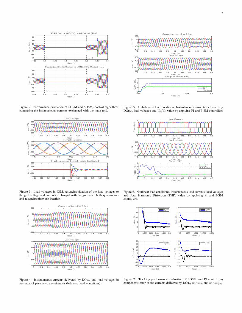
The transition time instants are imposed equal to tisl = 0.1 sand tgrid = 0.3 s, in which the microgrid is islanded fromand reconnected to the grid. Fig. 2 illustrates the currentsexchanged with the main grid, by applying both SOSM andSOSMc control, and it is apparent that the SOSMc algorithmbetter tracks the reference. Fig. 3 shows the three-phase loadvoltage and the resynchronization of the PCC voltage to thegrid voltage before reconnecting. Finally, the bottom of Fig.3 shows the currents exchanged with the main grid when boththe synchronization and resynchronization tools are inactive.

B. Unknown Load Dynamics

Consider the microgrid in IOM and in presence of balancedload condition. Then, from t = 0.15 s to t = 0.25 s a resistiveload, which absorbs an active power of 3 kW, is equally addedin the three phases, such that the resulting load is still balanced.Fig. 4 shows that during the load variation, the DGuM increasesthe delivered currents to supply the added load, while keepingthe load voltage equal to its reference value. Consider nowthat at t = 0.15 s the resulting load becomes unbalanced, i.e.,Ra = 5R, Rb = 4R, Rc = 2R and Lc = L are added in phasesa, b and c, respectively. In order to verify that the proposedcontrollers comply with the IEEE recommendations [45] forpower systems, the voltage imbalance ratio VN/VP (where VNand VP are the magnitudes of negative and positive sequencecomponents of load voltage) is calculated with the empiricalformula proposed in [46]. Fig. 5 shows that, when the 3-SM is applied, the voltage imbalance ratio settles to a valueapproximately equal to 2.5%, which is less than the maximum

7

0.05 0.1 0.15 0.2 0.25 0.3 0.35 0.4

−60

−40

−20

0

20

40

60

t is l tg r id

SOSM Control (GCOM), 3-SM Control (IOM)

time (s)

ig,abc(A

)

0.05 0.1 0.15 0.2 0.25 0.3 0.35 0.4

−60

−40

−20

0

20

40

60

t is l tg r id

Constrained SOSM Control (GCOM), 3-SM Control (IOM)

time (s)

ig,abc(A

)

Figure 2. Performance evaluation of SOSM and SOSMc control algorithms,comparing the instantaneous currents exchanged with the main grid.

0.1 0.12 0.14 0.16 0.18 0.2 0.22 0.24 0.26 0.28 0.3

−200

−100

0

100

200

Load Vol tages

t ime (s)

vabc(V

)

0.15 0.155 0.16 0.165 0.17 0.175 0.18−200

−100

0

100

200

Resynchroni zat i on

time (s)

vabc,vg,abc(V

)

0.25 0.26 0.27 0.28 0.29 0.3 0.31 0.32 0.33 0.34 0.35−200

−100

0

100

200

tg r id

Synchroni ze r and Resynchroni ze r deact ivated

time (s)

ig,abc(A

)

Figure 3. Load voltages in IOM, resynchronization of the load voltages tothe grid voltage and currents exchanged with the grid when both synchronizerand resynchronizer are inactive.

0.1 0.12 0.14 0.16 0.18 0.2 0.22 0.24 0.26 0.28 0.3−100

−50

0

50

100

Currents de l i ve red by DGuM

t ime (s)

it,abcM(A

)

0.1 0.12 0.14 0.16 0.18 0.2 0.22 0.24 0.26 0.28 0.3−200

−100

0

100

200

Load Vol tages

t ime (s)

vabc(V

)

Figure 4. Instantaneous currents delivered by DGuM and load voltages inpresence of parameter uncertainties (balanced load conditions).

0.1 0.12 0.14 0.16 0.18 0.2 0.22 0.24 0.26 0.28 0.3−100

−50

0

50

100

Currents de l i ve red by DGuM

t ime (s)

i t,a

bcM(A

)

0.1 0.12 0.14 0.16 0.18 0.2 0.22 0.24 0.26 0.28 0.3−200

−100

0

100

200

Load Vol tages

t ime (s)

vabc(V

)

0.15 0.2 0.25 0.30

2

4

6

t ime (s)

VN/VP

(%)

Vol tage imbalance rat i o

3 -SMP I(V N/V P )M

Figure 5. Unbalanced load condition. Instantaneous currents delivered byDGuM , load voltages and VN/VP value by applying PI and 3-SM controllers.

0.1 0.11 0.12 0.13 0.14 0.15 0.16 0.17 0.18 0.19 0.2−5

0

5Load Currents

t ime (s)

it,abcM(A

)

0.1 0.11 0.12 0.13 0.14 0.15 0.16 0.17 0.18 0.19 0.2−200

−100

0

100

200

Load Vol tages

t ime (s)

vabc(V

)

0.1 0.11 0.12 0.13 0.14 0.15 0.16 0.17 0.18 0.19 0.20

2

4

6

8

t ime (s)

THD

(%)

Vol tage THD

3 -SMP ITHDM

Figure 6. Nonlinear load conditions. Instantaneous load currents, load voltagesand Total Harmonic Distortion (THD) value by applying PI and 3-SMcontrollers.

0 0.002 0.004 0.006 0.008 0.01−5

0

5

10

15

20

t ime (s)

eItdM

(A)

SOSMP I

0.3 0.302 0.304 0.306 0.308−5

0

5

10

15

20

t ime (s)

eItdM

(A)

SOSMP I

0 0.002 0.004 0.006 0.008 0.01−15

−10

−5

0

5

10

15

20

25

t ime (s)

eItqM

(A)

SOSMP I

0.3 0.302 0.304 0.306 0.308−15

−10

−5

0

5

10

15

20

25

t ime (s)

eItqM

(A)

SOSMP I

Figure 7. Tracking performance evaluation of SOSM and PI control: dqcomponents error of the currents delivered by DGuM at t = t0 and at t = tgrid .

8

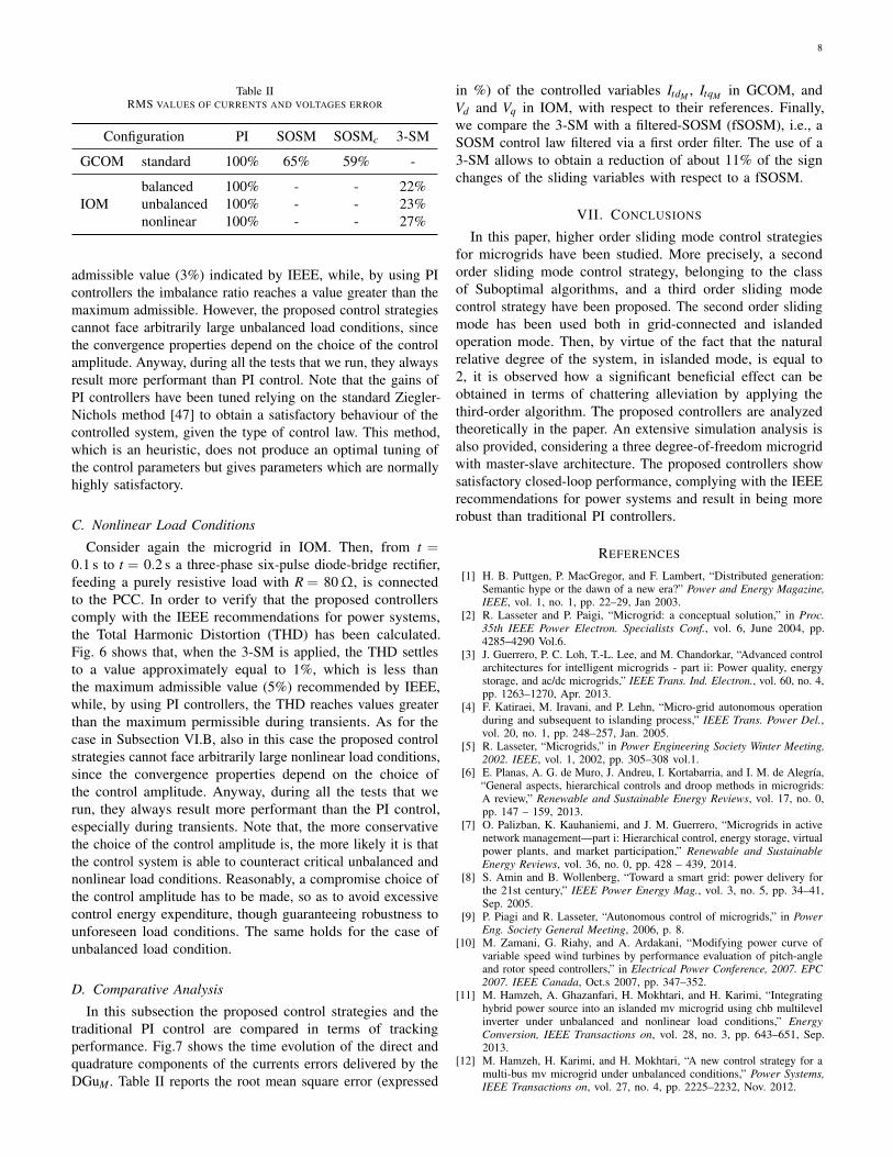
Table IIRMS VALUES OF CURRENTS AND VOLTAGES ERROR

Configuration PI SOSM SOSMc 3-SM

GCOM standard 100% 65% 59% -

IOMbalanced 100% - - 22%unbalanced 100% - - 23%nonlinear 100% - - 27%

admissible value (3%) indicated by IEEE, while, by using PIcontrollers the imbalance ratio reaches a value greater than themaximum admissible. However, the proposed control strategiescannot face arbitrarily large unbalanced load conditions, sincethe convergence properties depend on the choice of the controlamplitude. Anyway, during all the tests that we run, they alwaysresult more performant than PI control. Note that the gains ofPI controllers have been tuned relying on the standard Ziegler-Nichols method [47] to obtain a satisfactory behaviour of thecontrolled system, given the type of control law. This method,which is an heuristic, does not produce an optimal tuning ofthe control parameters but gives parameters which are normallyhighly satisfactory.

C. Nonlinear Load Conditions

Consider again the microgrid in IOM. Then, from t =0.1 s to t = 0.2 s a three-phase six-pulse diode-bridge rectifier,feeding a purely resistive load with R = 80Ω, is connectedto the PCC. In order to verify that the proposed controllerscomply with the IEEE recommendations for power systems,the Total Harmonic Distortion (THD) has been calculated.Fig. 6 shows that, when the 3-SM is applied, the THD settlesto a value approximately equal to 1%, which is less thanthe maximum admissible value (5%) recommended by IEEE,while, by using PI controllers, the THD reaches values greaterthan the maximum permissible during transients. As for thecase in Subsection VI.B, also in this case the proposed controlstrategies cannot face arbitrarily large nonlinear load conditions,since the convergence properties depend on the choice ofthe control amplitude. Anyway, during all the tests that werun, they always result more performant than the PI control,especially during transients. Note that, the more conservativethe choice of the control amplitude is, the more likely it is thatthe control system is able to counteract critical unbalanced andnonlinear load conditions. Reasonably, a compromise choice ofthe control amplitude has to be made, so as to avoid excessivecontrol energy expenditure, though guaranteeing robustness tounforeseen load conditions. The same holds for the case ofunbalanced load condition.

D. Comparative Analysis

In this subsection the proposed control strategies and thetraditional PI control are compared in terms of trackingperformance. Fig.7 shows the time evolution of the direct andquadrature components of the currents errors delivered by theDGuM . Table II reports the root mean square error (expressed

in %) of the controlled variables ItdM , ItqM in GCOM, andVd and Vq in IOM, with respect to their references. Finally,we compare the 3-SM with a filtered-SOSM (fSOSM), i.e., aSOSM control law filtered via a first order filter. The use of a3-SM allows to obtain a reduction of about 11% of the signchanges of the sliding variables with respect to a fSOSM.

VII. CONCLUSIONS

In this paper, higher order sliding mode control strategiesfor microgrids have been studied. More precisely, a secondorder sliding mode control strategy, belonging to the classof Suboptimal algorithms, and a third order sliding modecontrol strategy have been proposed. The second order slidingmode has been used both in grid-connected and islandedoperation mode. Then, by virtue of the fact that the naturalrelative degree of the system, in islanded mode, is equal to2, it is observed how a significant beneficial effect can beobtained in terms of chattering alleviation by applying thethird-order algorithm. The proposed controllers are analyzedtheoretically in the paper. An extensive simulation analysis isalso provided, considering a three degree-of-freedom microgridwith master-slave architecture. The proposed controllers showsatisfactory closed-loop performance, complying with the IEEErecommendations for power systems and result in being morerobust than traditional PI controllers.

REFERENCES

[1] H. B. Puttgen, P. MacGregor, and F. Lambert, “Distributed generation:Semantic hype or the dawn of a new era?” Power and Energy Magazine,IEEE, vol. 1, no. 1, pp. 22–29, Jan 2003.

[2] R. Lasseter and P. Paigi, “Microgrid: a conceptual solution,” in Proc.35th IEEE Power Electron. Specialists Conf., vol. 6, June 2004, pp.4285–4290 Vol.6.

[3] J. Guerrero, P. C. Loh, T.-L. Lee, and M. Chandorkar, “Advanced controlarchitectures for intelligent microgrids - part ii: Power quality, energystorage, and ac/dc microgrids,” IEEE Trans. Ind. Electron., vol. 60, no. 4,pp. 1263–1270, Apr. 2013.

[4] F. Katiraei, M. Iravani, and P. Lehn, “Micro-grid autonomous operationduring and subsequent to islanding process,” IEEE Trans. Power Del.,vol. 20, no. 1, pp. 248–257, Jan. 2005.

[5] R. Lasseter, “Microgrids,” in Power Engineering Society Winter Meeting,2002. IEEE, vol. 1, 2002, pp. 305–308 vol.1.

[6] E. Planas, A. G. de Muro, J. Andreu, I. Kortabarria, and I. M. de Alegría,“General aspects, hierarchical controls and droop methods in microgrids:A review,” Renewable and Sustainable Energy Reviews, vol. 17, no. 0,pp. 147 – 159, 2013.

[7] O. Palizban, K. Kauhaniemi, and J. M. Guerrero, “Microgrids in activenetwork management—part i: Hierarchical control, energy storage, virtualpower plants, and market participation,” Renewable and SustainableEnergy Reviews, vol. 36, no. 0, pp. 428 – 439, 2014.

[8] S. Amin and B. Wollenberg, “Toward a smart grid: power delivery forthe 21st century,” IEEE Power Energy Mag., vol. 3, no. 5, pp. 34–41,Sep. 2005.

[9] P. Piagi and R. Lasseter, “Autonomous control of microgrids,” in PowerEng. Society General Meeting, 2006, p. 8.

[10] M. Zamani, G. Riahy, and A. Ardakani, “Modifying power curve ofvariable speed wind turbines by performance evaluation of pitch-angleand rotor speed controllers,” in Electrical Power Conference, 2007. EPC2007. IEEE Canada, Oct.s 2007, pp. 347–352.

[11] M. Hamzeh, A. Ghazanfari, H. Mokhtari, and H. Karimi, “Integratinghybrid power source into an islanded mv microgrid using chb multilevelinverter under unbalanced and nonlinear load conditions,” EnergyConversion, IEEE Transactions on, vol. 28, no. 3, pp. 643–651, Sep.2013.

[12] M. Hamzeh, H. Karimi, and H. Mokhtari, “A new control strategy for amulti-bus mv microgrid under unbalanced conditions,” Power Systems,IEEE Transactions on, vol. 27, no. 4, pp. 2225–2232, Nov. 2012.

9

[13] M. Babazadeh and H. Karimi, “A robust two-degree-of-freedom controlstrategy for an islanded microgrid,” IEEE Trans. Power Del., vol. 28,no. 3, pp. 1339–1347, Jul. 2013.

[14] H. Karimi, H. Nikkhajoei, and R. Iravani, “Control of an electronically-coupled distributed resource unit subsequent to an islanding event,” IEEETrans. Power Del., vol. 23, no. 1, pp. 493–501, Jan. 2008.

[15] H. Karimi, E. Davison, and R. Iravani, “Multivariable servomechanismcontroller for autonomous operation of a distributed generation unit:Design and performance evaluation,” IEEE Trans. Power Syst., vol. 25,no. 2, pp. 853–865, May 2010.

[16] K. De Brabandere, B. Bolsens, J. Van den Keybus, A. Woyte, J. Driesen,and R. Belmans, “A voltage and frequency droop control method forparallel inverters,” IEEE Trans. Power Electronics, vol. 22, no. 4, pp.1107–1115, July 2007.

[17] C.-T. Lee, C.-C. Chu, and P.-T. Cheng, “A new droop control methodfor the autonomous operation of distributed energy resource interfaceconverters,” IEEE Trans. Power Electronics, vol. 28, no. 4, pp. 1980–1993,April 2013.

[18] R. Palma-Behnke, C. Benavides, F. Lanas, B. Severino, L. Reyes,J. Llanos, and D. Saez, “A microgrid energy management system basedon the rolling horizon strategy,” Smart Grid, IEEE Transactions on,vol. 4, no. 2, pp. 996–1006, June 2013.

[19] A. Parisio, E. Rikos, and L. Glielmo, “A Model Predictive ControlApproach to Microgrid Operation Optimization,” IIEEE Trans. ControlSyst. Techn., vol. 22, no. 5, pp. 1813–1827, 2014.

[20] D. Salomonsson, L. Soder, and A. Sannino, “An adaptive control systemfor a dc microgrid for data centers,” IEEE Trans. Industry Applications,vol. 44, no. 6, pp. 1910–1917, Nov 2008.

[21] A. Bidram, A. Davoudi, F. Lewis, and S. S. Ge, “Distributed adaptivevoltage control of inverter-based microgrids,” IEEE Trans. EnergyConversion, vol. 29, no. 4, pp. 862–872, Dec 2014.

[22] T. Hornik and Q.-C. Zhong, “A current-control strategy for voltage-sourceinverters in microgrids based on h∞ and repetitive control,” IEEE Trans.Power Electronics, vol. 26, no. 3, pp. 943–952, March 2011.

[23] S. Riverso, F. Sarzo, and G. Ferrari-Trecate, “Plug-and-play voltage andfrequency control of islanded microgrids with meshed topology,” CoRR,vol. abs/1405.2421, 2014.

[24] V. I. Utkin, Sliding Modes in Optimization and Control Problems. NewYork: Springer Verlag, 1992.

[25] C. Edwards and S. K. Spurgen, Sliding Mode Control: Theory andApplications. London, UK: Taylor and Francis, 1998.

[26] M. Rubagotti, A. Estrada, F. Castanos, A. Ferrara, and L. Fridman,“Integral sliding mode control for nonlinear systems with matched andunmatched perturbations,” Automatic Control, IEEE Transactions on,vol. 56, no. 11, pp. 2699–2704, Nov 2011.

[27] L. Fridman, “Singularly perturbed analysis of chattering in relay controlsystems,” IEEE Trans. Automat. Control, vol. 47, no. 12, pp. 2079 –2084, Dec. 2002.

[28] I. Boiko, L. Fridman, A. Pisano, and E. Usai, “Analysis of chattering insystems with second-order sliding modes,” IEEE Trans. Automat. Control,vol. 52, no. 11, pp. 2085 –2102, Nov. 2007.

[29] A. Levant, “Chattering analysis,” IEEE Trans. Automat. Control, vol. 55,no. 6, pp. 1380 –1389, Jun. 2010.

[30] F. Dinuzzo and A. Ferrara, “Higher order sliding mode controllers withoptimal reaching,” IEEE Trans. Automat. Control, vol. 54, no. 9, pp.2126 –2136, Sep. 2009.

[31] G. Bartolini, A. Ferrara, and E. Usai, “Chattering avoidance by second-order sliding mode control,” IEEE Trans. Automat. Control, vol. 43,no. 2, pp. 241–246, Feb. 1998.

[32] ——, “Output tracking control of uncertain nonlinear second-ordersystems,” Automatica, vol. 33, no. 12, pp. 2203 – 2212, Dec. 1997.

[33] G. Bartolini, A. Ferrara, E. Usai, and V. Utkin, “On multi-input chattering-free second-order sliding mode control,” IEEE Trans. Automat. Control,vol. 45, no. 9, pp. 1711–1717, Sep. 2000.

[34] G. Bartolini, A. Ferrara, and E. Usai, “On boundary layer dimensionreduction in sliding mode control of siso uncertain nonlinear systems,”in Proc. IEEE Int. Conf. Control Applications, vol. 1, Trieste, Italy, Sep.1998, pp. 242 –247 vol.1.

[35] M. Cucuzzella, G. P. Incremona, and A. Ferrara, “Master-slave secondorder sliding mode control for microgrids,” in Proc. IEEE AmericanControl Conf. (ACC), Jul. 2015.

[36] ——, “Third order sliding mode voltage control in microgrids,” in Proc.IEEE European Control Conf. (ECC), Jul. 2015.

[37] R. H. Park, “Two-reaction theory of synchronous machines - generalizedmethod of analysis - part i,” Trans. American Instit. Electr. Eng., vol. 48,no. 3, pp. 716 – 727, 1929.

[38] R. Vijayan, S. Ch, and R. Roy, “Dynamic modeling of microgrid forgrid connected and intentional islanding operation,” in Proc. Advancesin Power Conv. and Energy Techn. Int. Conf., Aug. 2012, pp. 1–6.

[39] I. Balaguer, Q. Lei, S. Yang, U. Supatti, and F. Z. Peng, “Control forgrid-connected and intentional islanding operations of distributed powergeneration,” IEEE Trans. Ind. Electron., vol. 58, no. 1, pp. 147–157, Jan.2011.

[40] I. Boiko, “Analysis of chattering in sliding mode control systems withcontinuous boundary layer approximation of discontinuous control,” inProc. American Control Conf., San Francisco, CA, USA, Jul. 2011, pp.757 –762.

[41] H. Lee and V. I. Utkin, “Chattering suppression methods in sliding modecontrol systems,” Annual Reviews in Control, vol. 31, no. 2, pp. 179 –188, Oct. 2007.

[42] M. Rubagotti and A. Ferrara, “Second order sliding mode control of aperturbed double integrator with state constraints,” in Proc. AmericanControl Conf., Baltimora, MD, USA, Jun. 2010, pp. 985–990.

[43] A. F. Filippov and F. M. Arscott, Differential Equations with Discontin-uous Right-hand Sides: Control Systems. Springer, 1988, vol. 18.

[44] J. Aubin and A. Cellina, Differential Inclusions. Springer Verlag Berlin/ Heidelberg, 1984.

[45] IEEE, “Recommended practice for monitoring electric power quality,”IEEE Std 1159-2009 (Revision of IEEE Std 1159-1995), pp. c1–81, Jun.2009.

[46] P. Pillay and M. Manyage, “Definitions of voltage unbalance,” IEEEPower Engineering Review, vol. 21, no. 5, pp. 50–51, 2001.

[47] J. G. Ziegler and N. B. Nichols, “Optimum settings for automaticcontrollers,” ASME. J. Dyn. Sys., vol. 64, no. 759, 1942.

Michele Cucuzzella received the Bachelor Degree(with honor) in Industrial Engineering and the MasterDegree (with honor) in electric Engineering fromthe University of Pavia, Italy in 2012 and 2014,respectively. Currently he is a Ph.D. Student inElectronics, Computer Science and electric Engineer-ing for the Identification and Control of DynamicSystems Laboratory at the University of Pavia underthe supervision of Professor Antonella Ferrara. Hisresearch activities are mainly in the area of VariableStructure and Sliding Mode Control and of Event-

Triggered Control with application to the Microgrids.

Gian Paolo Incremona received the Master Degree(with honor) in electric Engineering from the Uni-versity of Pavia, Italy in 2012. He was a student ofthe Almo Collegio Borromeo of Pavia, and of theclass of Science and Technology of the Institute forAdvanced Studies IUSS of Pavia. He is now a Ph.D.Candidate in Electronics, electric and ComputerEngineering at the Identification and Control ofDynamic Systems Laboratory of the University ofPavia under the supervision of Professor AntonellaFerrara. His research deals with industrial robotics,

real-time physical systems, optimal control and variable structure controlmethods of sliding mode type.

Antonella Ferrara is Full Professor of AutomaticControl at the University of Pavia. Her researchdeals with sliding mode and nonlinear control withapplication to traffic, automotive and robotics. Shehas authored/co-authored more than 300 papers,including more than 90 journal papers. She wasAssociate Editor of the IEEE Transactions on ControlSystems Technology and of the IEEE Transactionson Automatic Control. Since January 2014, sheis Associate Editor of the IEEE Control SystemsMagazine. She is Senior Member of the IEEE Control

Systems Society, and, among others, member of the IEEE Technical Committeeon Variable Structure and Sliding Mode Control, and of the IFAC TechnicalCommittee on Transportation Systems. Since July 2013 she is Chair of theWomen in Control Standing Committee of the Control Systems Society.