Design of the TELSIS trial

Martin BlandProfessor of Health Statistics

Department of Health SciencesUniversity of York

with Dawn Dowding and Helen Cheyne

www-users.york.ac.uk/~mb55/

TELSIS:

The Early Labour Study In Scotland

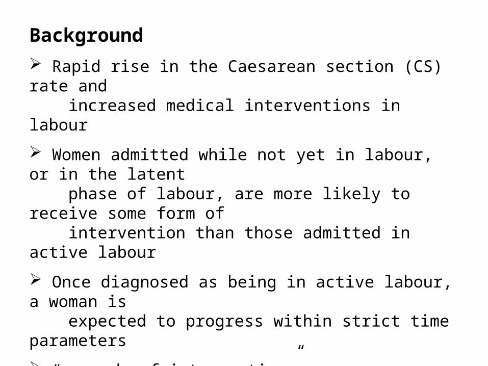
Background

Rapid rise in the Caesarean section (CS) rate and increased medical interventions in labour

Women admitted while not yet in labour, or in the latent phase of labour, are more likely to receive some form of intervention than those admitted in active labour

Once diagnosed as being in active labour, a woman is expected to progress within strict time parameters

“cascade of intervention”

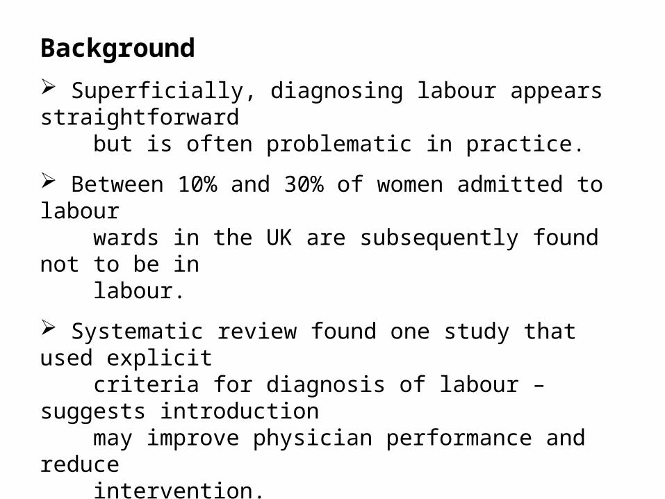
Background

Superficially, diagnosing labour appears straightforward but is often problematic in practice.

Between 10% and 30% of women admitted to labour wards in the UK are subsequently found not to be in labour.

Systematic review found one study that used explicit criteria for diagnosis of labour – suggests introduction may improve physician performance and reduce intervention.

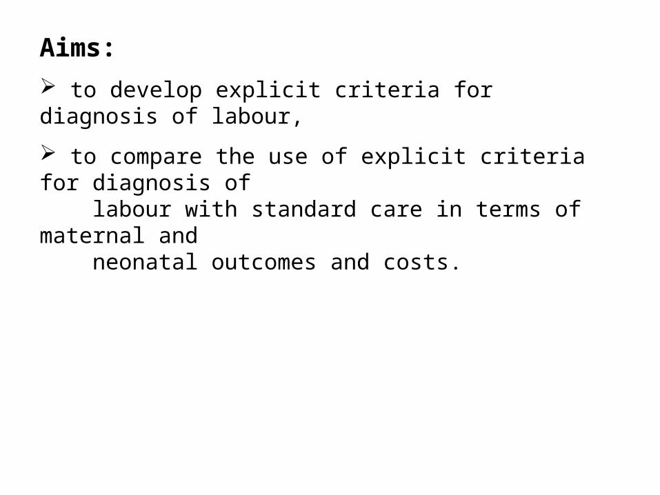
Aims:

to develop explicit criteria for diagnosis of labour,

to compare the use of explicit criteria for diagnosis of labour with standard care in terms of maternal and neonatal outcomes and costs.

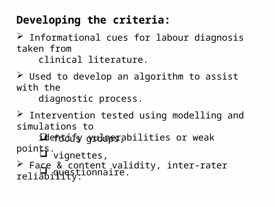
Developing the criteria:

Informational cues for labour diagnosis taken from clinical literature.

Used to develop an algorithm to assist with the diagnostic process.

Intervention tested using modelling and simulations to identify vulnerabilities or weak points.

Face & content validity, inter-rater reliability:

focus groups,

vignettes,

questionnaire.

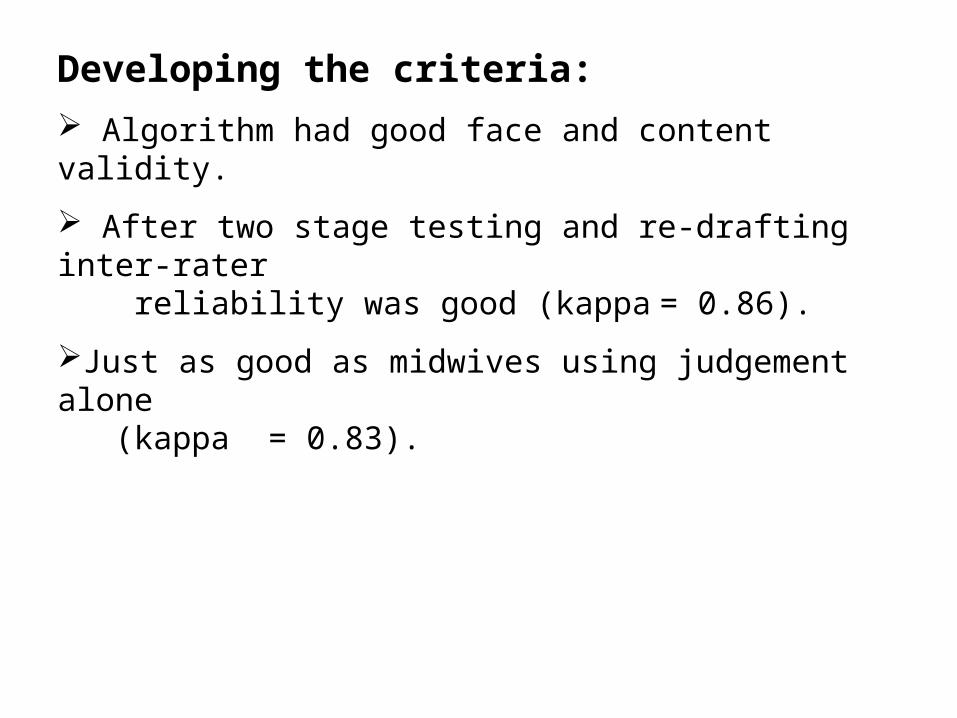
Developing the criteria:

Algorithm had good face and content validity.

After two stage testing and re-drafting inter-rater reliability was good (kappa = 0.86).

Just as good as midwives using judgement alone (kappa = 0.83).

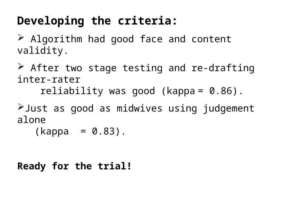
Developing the criteria:

Algorithm had good face and content validity.

After two stage testing and re-drafting inter-rater reliability was good (kappa = 0.86).

Just as good as midwives using judgement alone (kappa = 0.83).

Ready for the trial!

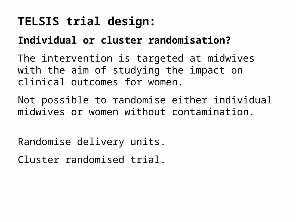
TELSIS trial design:

Individual or cluster randomisation?

The intervention is targeted at midwives with the aim of studying the impact on clinical outcomes for women.

Not possible to randomise either individual midwives or women without contamination.

Randomise delivery units.

Cluster randomised trial.

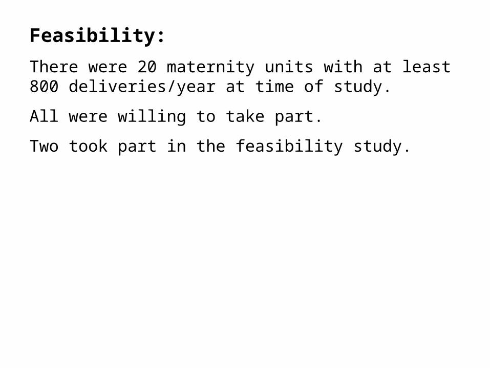
Feasibility:

There were 20 maternity units with at least 800 deliveries/year at time of study.

All were willing to take part.

Two took part in the feasibility study.

Feasibility:

Test of feasibility of key components of the main trial in two delivery units:

consent,

compliance,

study materials,

training needs.

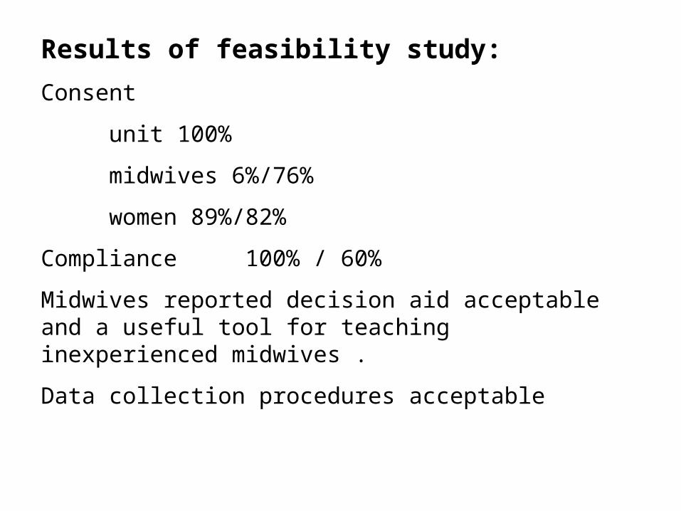
Results of feasibility study:

Consent

unit 100%

midwives 6%/76%

women 89%/82%

Compliance 100% / 60%

Midwives reported decision aid acceptable and a useful tool for teaching inexperienced midwives .

Data collection procedures acceptable

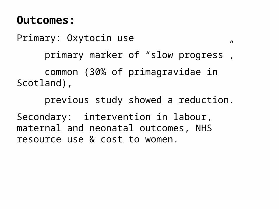
Outcomes:

Primary: Oxytocin use

primary marker of “slow progress”,

common (30% of primagravidae in Scotland),

previous study showed a reduction.

Secondary: intervention in labour, maternal and neonatal outcomes, NHS resource use & cost to women.

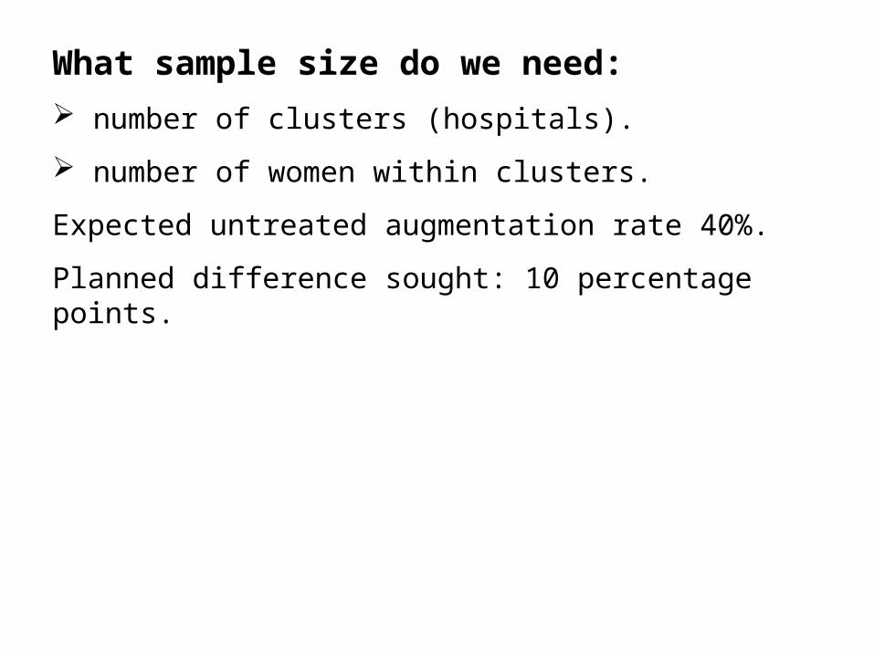
What sample size do we need:

number of clusters (hospitals).

number of women within clusters.

Expected untreated augmentation rate 40%.

Planned difference sought: 10 percentage points.

What sample size do we need?

number of clusters (hospitals).

number of women within clusters.

Expected untreated augmentation rate 40%.

Planned difference sought: 10 percentage points.

In an individually randomised trial, to detect a difference between 40% and 30% with power 0.90 would need 476 per group.

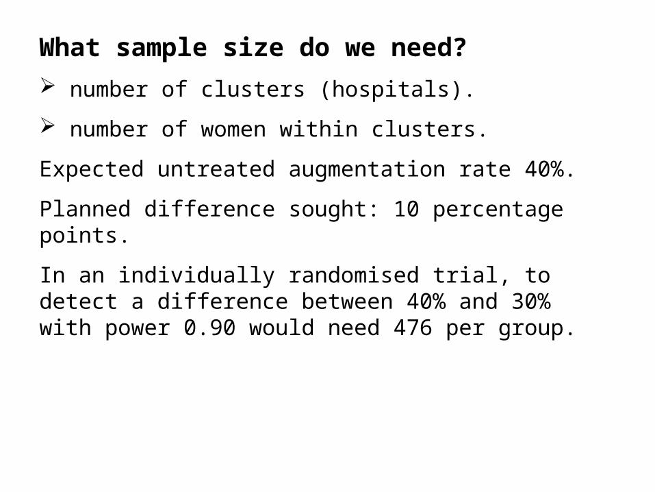
What sample size do we need?

number of clusters (hospitals).

number of women within clusters.

Expected untreated augmentation rate 40%.

Planned difference sought: 10 percentage points.

In an individually randomised trial, to detect a difference between 40% and 30% with power 0.90 would need 476 per group.

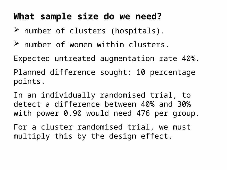
For a cluster randomised trial, we must multiply this by the design effect.

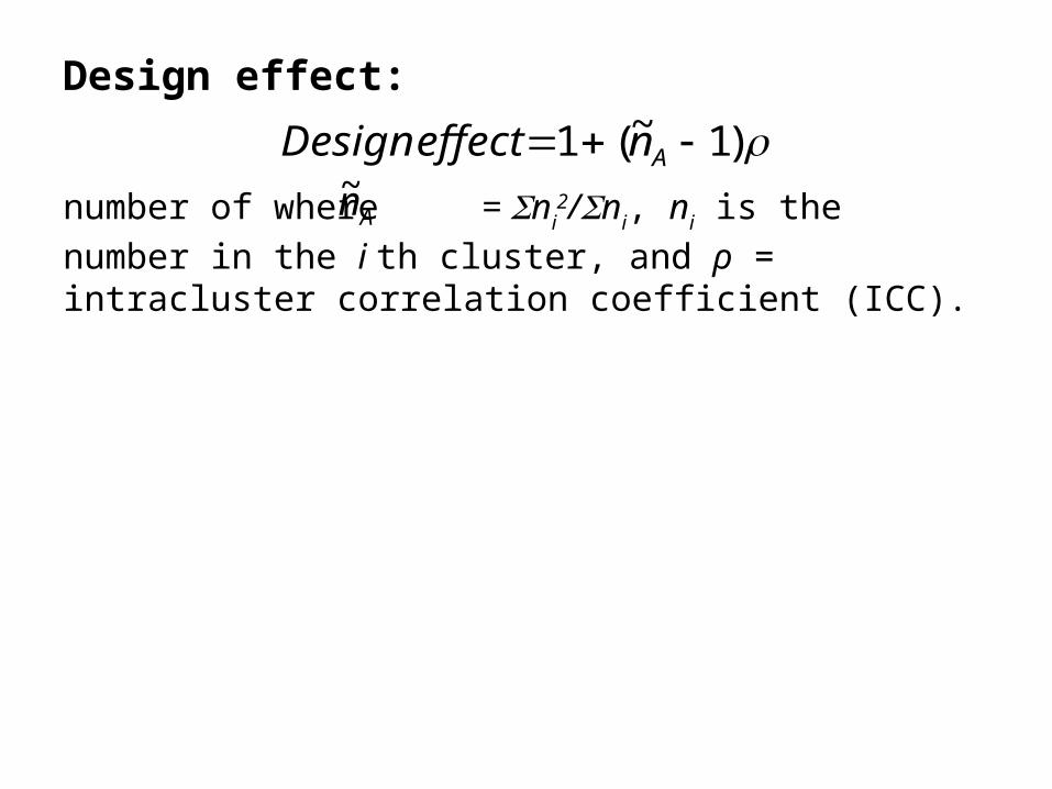
Design effect:

number of where = ni2/ni, ni is the number in the i th

cluster, and ρ = intracluster correlation coefficient (ICC).

)1~(1 AneffectDesign

An~

Design effect:

number of where = ni2/ni, ni is the number in the i th

cluster, and ρ = intracluster correlation coefficient (ICC).

Question: what value should we use for ICC?

)1~(1 AneffectDesign

An~

Design effect:

number of where = ni2/ni, ni is the number in the i th

cluster, and ρ = intracluster correlation coefficient (ICC).

Question: what value should we use for ICC?

Answer: pilot study data.

)1~(1 AneffectDesign

An~

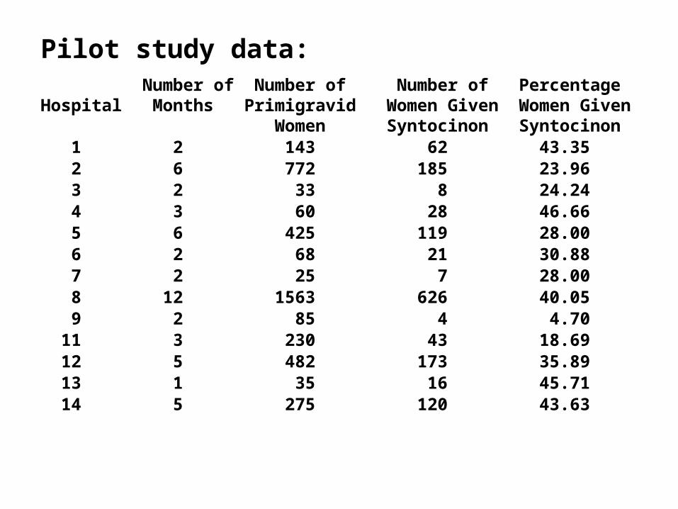
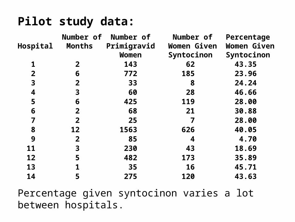
Pilot study data: Number of Number of Number of PercentageHospital Months Primigravid Women Given Women Given Women Syntocinon Syntocinon 1 2 143 62 43.35 2 6 772 185 23.96 3 2 33 8 24.24 4 3 60 28 46.66 5 6 425 119 28.00 6 2 68 21 30.88 7 2 25 7 28.00 8 12 1563 626 40.05 9 2 85 4 4.70 11 3 230 43 18.69 12 5 482 173 35.89 13 1 35 16 45.71 14 5 275 120 43.63

Pilot study data: Number of Number of Number of PercentageHospital Months Primigravid Women Given Women Given Women Syntocinon Syntocinon 1 2 143 62 43.35 2 6 772 185 23.96 3 2 33 8 24.24 4 3 60 28 46.66 5 6 425 119 28.00 6 2 68 21 30.88 7 2 25 7 28.00 8 12 1563 626 40.05 9 2 85 4 4.70 11 3 230 43 18.69 12 5 482 173 35.89 13 1 35 16 45.71 14 5 275 120 43.63

Percentage given syntocinon varies a lot between hospitals.

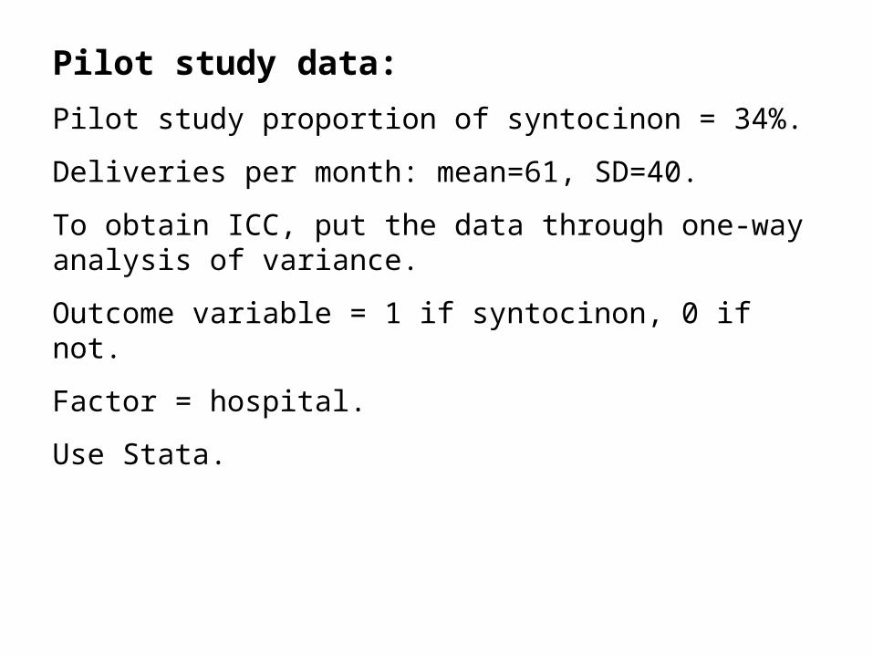
Pilot study data:

Pilot study proportion of syntocinon = 34%.

Deliveries per month: mean=61, SD=40.

To obtain ICC, put the data through one-way analysis of variance.

Outcome variable = 1 if syntocinon, 0 if not.

Factor = hospital.

Use Stata.

Pilot study data:. loneway usesyn hospital

One-way Analysis of Variance for usesyn: Number of obs = 4196 R-squared = 0.0358

Source SS df MS F Prob > F------------------------------------------------------------------Between hospital 33.550954 12 2.7959128 12.95 0.0000Within hospital 903.29557 4183 .21594443------------------------------------------------------------------Total 936.84652 4195 .22332456

Intraclass Asy. correlation S.E. [95% Conf. Interval] ------------------------------------------------ 0.04124 0.02588 0.00000 0.09196

Estimated SD of hospital effect .096372 Estimated SD within hospital .4646982 Est. reliability of a hospital mean 0.92276 (evaluated at n=277.79)

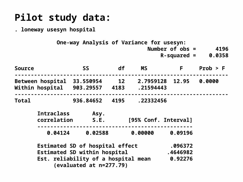
Pilot study data:. loneway usesyn hospital

One-way Analysis of Variance for usesyn: Number of obs = 4196 R-squared = 0.0358

Source SS df MS F Prob > F------------------------------------------------------------------Between hospital 33.550954 12 2.7959128 12.95 0.0000Within hospital 903.29557 4183 .21594443------------------------------------------------------------------Total 936.84652 4195 .22332456

Intraclass Asy. correlation S.E. [95% Conf. Interval] ------------------------------------------------ 0.04124 0.02588 0.00000 0.09196

Estimated SD of hospital effect .096372 Estimated SD within hospital .4646982 Est. reliability of a hospital mean 0.92276 (evaluated at n=277.79)

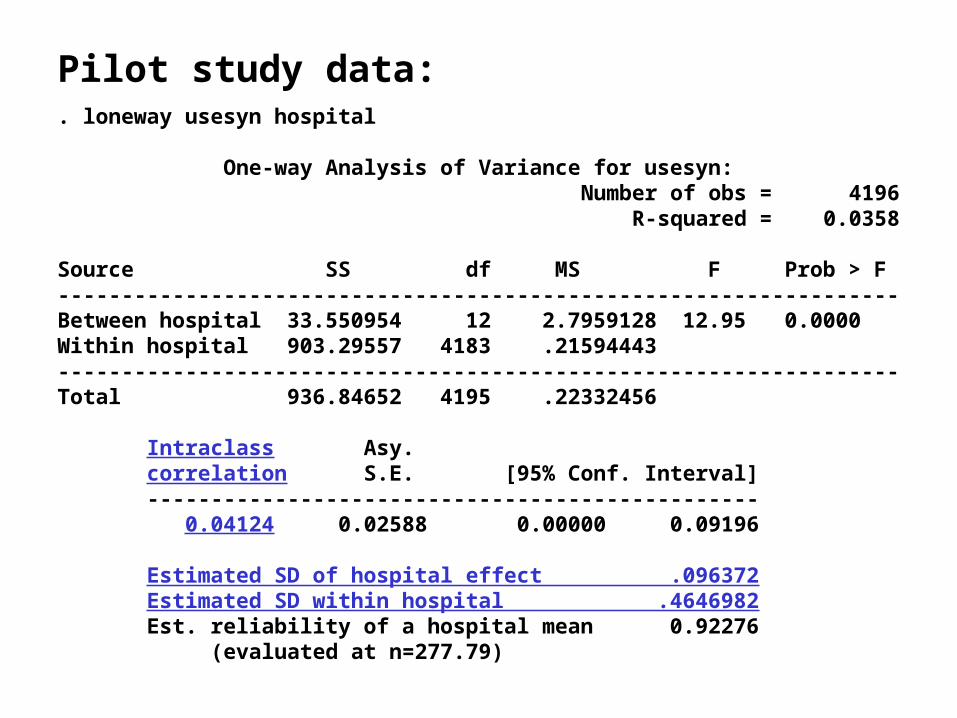
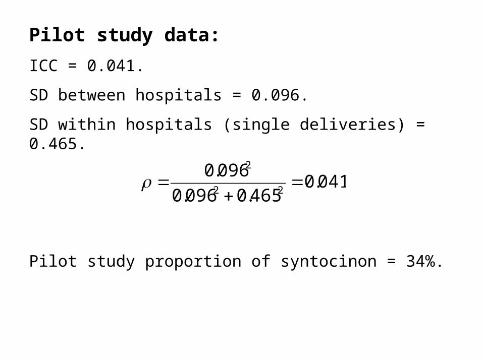
Pilot study data:

ICC = 0.041.

SD between hospitals = 0.096.

SD within hospitals (single deliveries) = 0.465.

Pilot study proportion of syntocinon = 34%.

041.0465.0096.0

096.022

2

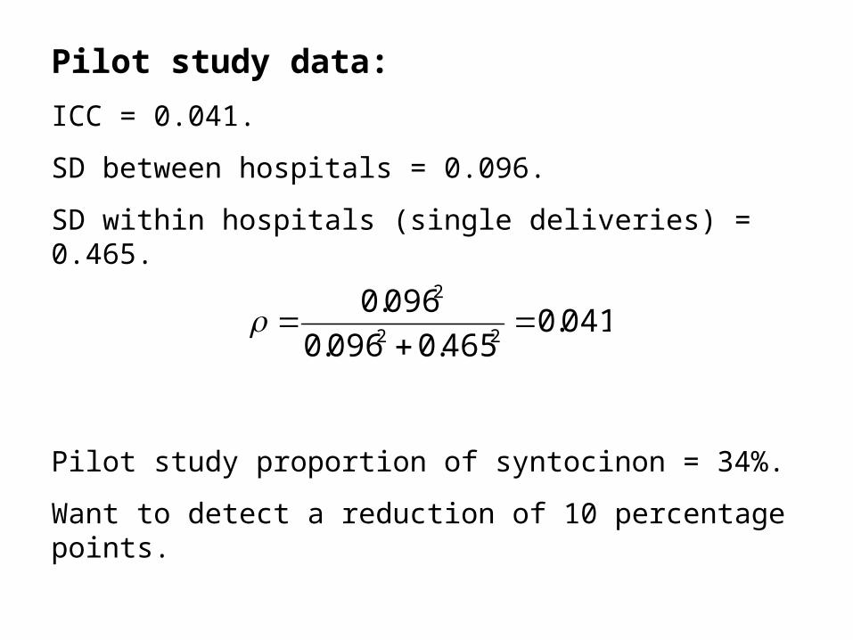
Pilot study data:

ICC = 0.041.

SD between hospitals = 0.096.

SD within hospitals (single deliveries) = 0.465.

Pilot study proportion of syntocinon = 34%.

Want to detect a reduction of 10 percentage points.

041.0465.0096.0

096.022

2

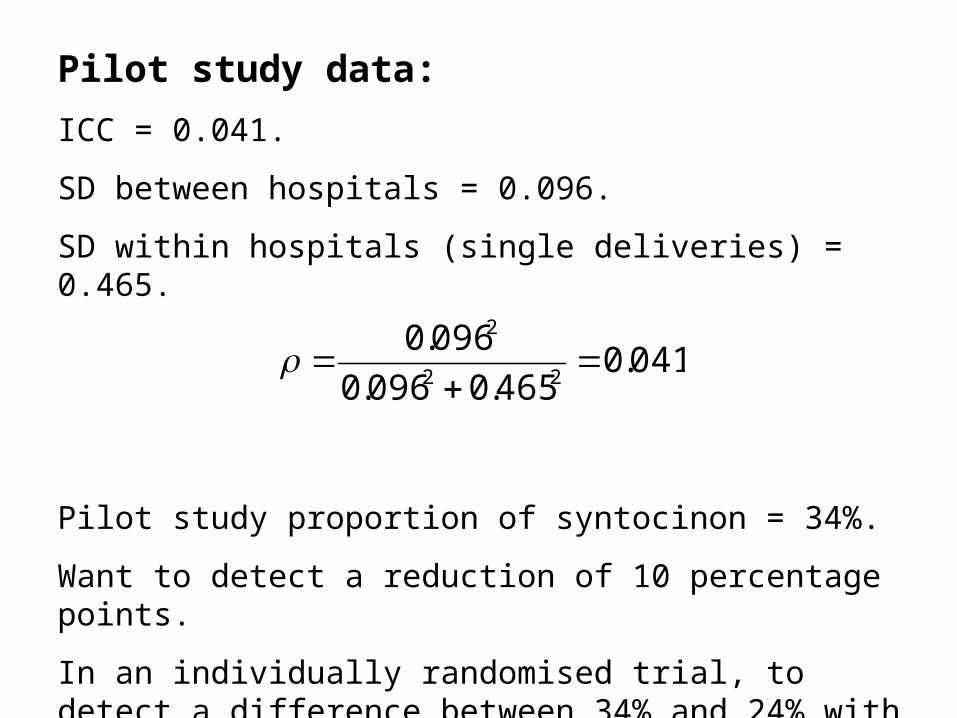
Pilot study data:

ICC = 0.041.

SD between hospitals = 0.096.

SD within hospitals (single deliveries) = 0.465.

Pilot study proportion of syntocinon = 34%.

Want to detect a reduction of 10 percentage points.

In an individually randomised trial, to detect a difference between 34% and 24% with power 0.90 would need 431 per group.

041.0465.0096.0

096.022

2

Pilot study data:

where = ni2/ni, ni is the number in the i th cluster, and ρ

= intracluster correlation coefficient (ICC).

We have ρ = 0.041.

For the design effect, we need . An~

)1~(1 AneffectDesign

An~

Pilot study data: Number of Number of Number of Number ofHospital months primigravid women per women per women month, ni month2, ni

2

1 2 143 71.50 5112.25 2 6 772 128.67 16555.11 3 2 33 16.50 272.25 4 3 60 20.00 400.00 5 6 425 70.83 5017.36 6 2 68 34.00 1156.00 7 2 25 12.50 156.25 8 12 1563 130.25 16965.06 9 2 85 42.50 1806.25 11 5 482 96.40 9292.96 12 1 35 35.00 1225.00 13 5 275 55.00 3025.00

Total 789.82 66861.28

Mean 65.8

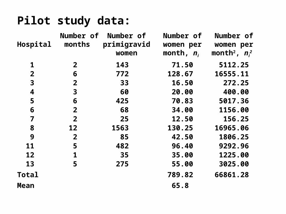
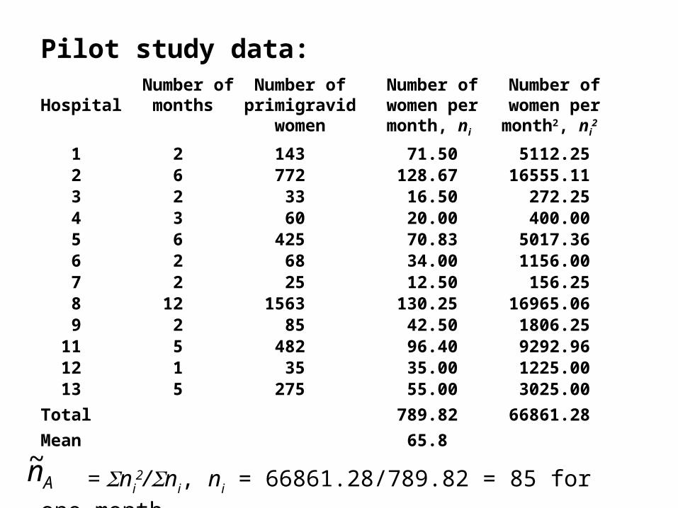
Pilot study data: Number of Number of Number of Number ofHospital months primigravid women per women per women month, ni month2, ni

2

1 2 143 71.50 5112.25 2 6 772 128.67 16555.11 3 2 33 16.50 272.25 4 3 60 20.00 400.00 5 6 425 70.83 5017.36 6 2 68 34.00 1156.00 7 2 25 12.50 156.25 8 12 1563 130.25 16965.06 9 2 85 42.50 1806.25 11 5 482 96.40 9292.96 12 1 35 35.00 1225.00 13 5 275 55.00 3025.00

Total 789.82 66861.28

Mean 65.8

= ni2/ni, ni = 66861.28/789.82 = 85 for one month.An~

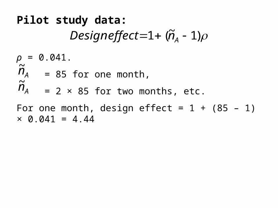
Pilot study data:

ρ = 0.041.

= 85 for one month,

= 2 × 85 for two months, etc.

For one month, design effect = 1 + (85 – 1) × 0.041 = 4.44

An~

)1~(1 AneffectDesign

An~

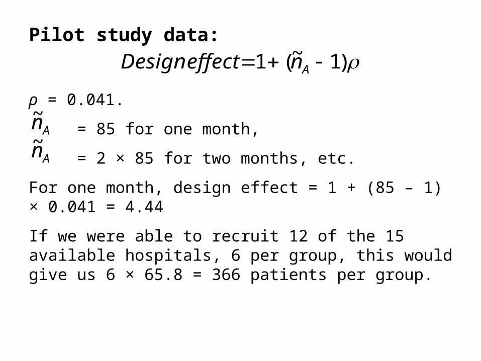
Pilot study data:

ρ = 0.041.

= 85 for one month,

= 2 × 85 for two months, etc.

For one month, design effect = 1 + (85 – 1) × 0.041 = 4.44

If we were able to recruit 12 of the 15 available hospitals, 6 per group, this would give us 6 × 65.8 = 366 patients per group.

An~

)1~(1 AneffectDesign

An~

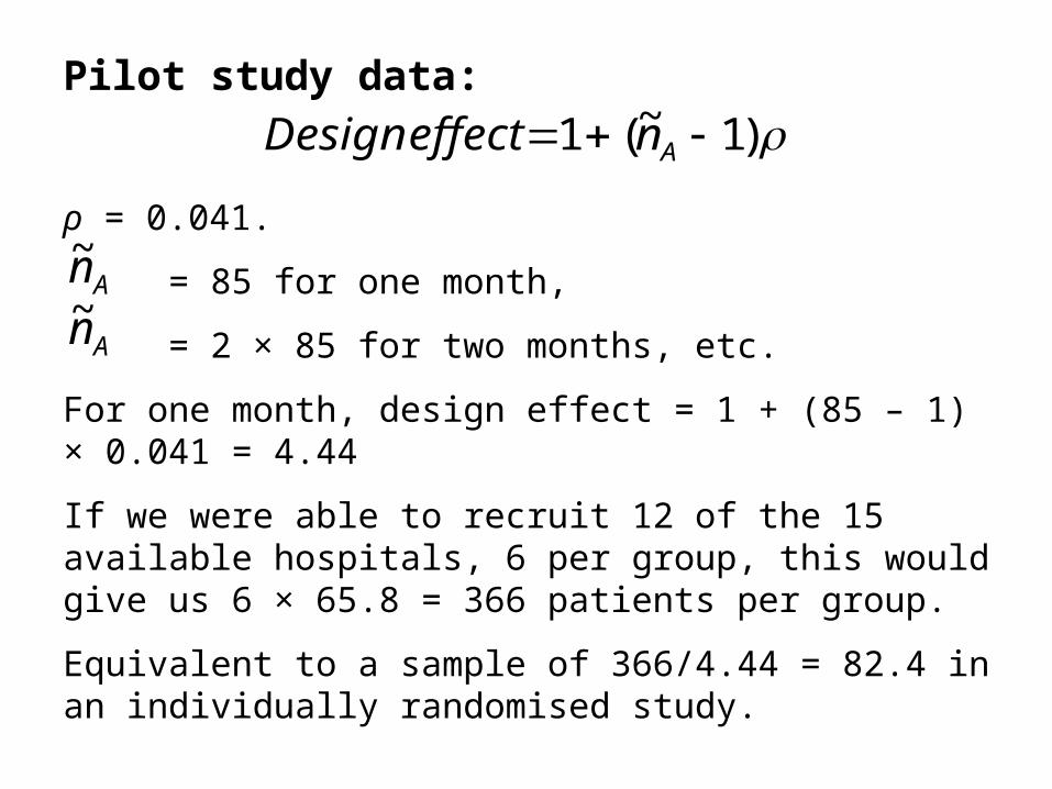
Pilot study data:

ρ = 0.041.

= 85 for one month,

= 2 × 85 for two months, etc.

For one month, design effect = 1 + (85 – 1) × 0.041 = 4.44

If we were able to recruit 12 of the 15 available hospitals, 6 per group, this would give us 6 × 65.8 = 366 patients per group.

Equivalent to a sample of 366/4.44 = 82.4 in an individually randomised study.

An~

)1~(1 AneffectDesign

An~

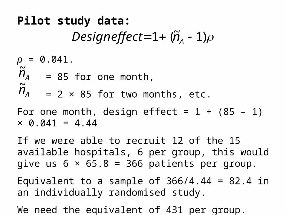
Pilot study data:

ρ = 0.041.

= 85 for one month,

= 2 × 85 for two months, etc.

For one month, design effect = 1 + (85 – 1) × 0.041 = 4.44

If we were able to recruit 12 of the 15 available hospitals, 6 per group, this would give us 6 × 65.8 = 366 patients per group.

Equivalent to a sample of 366/4.44 = 82.4 in an individually randomised study.

We need the equivalent of 431 per group.

An~

)1~(1 AneffectDesign

An~

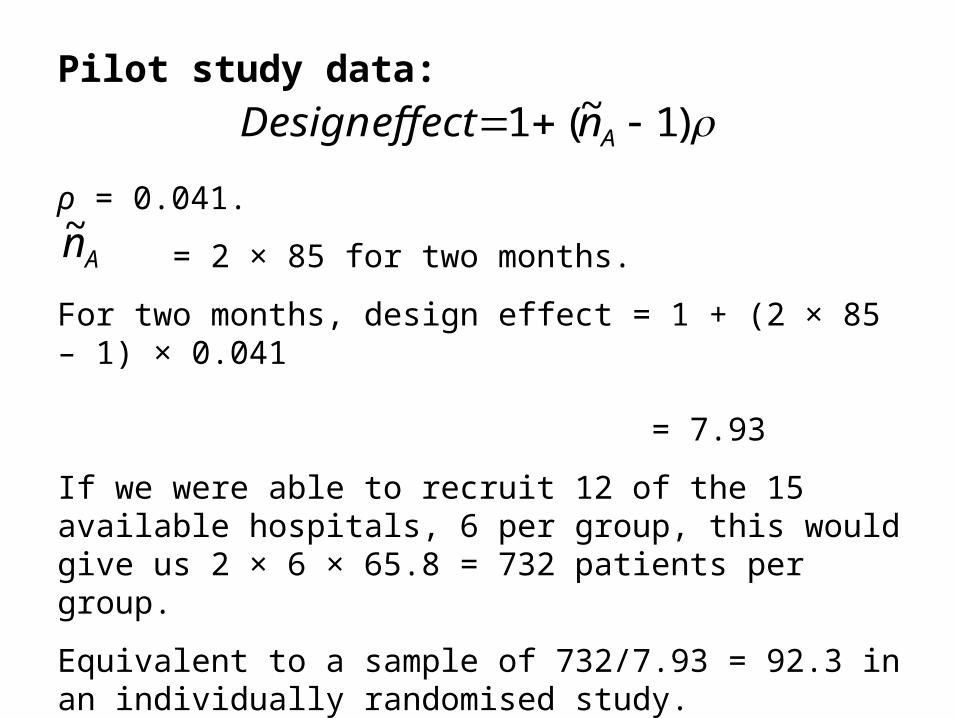
Pilot study data:

ρ = 0.041.

= 2 × 85 for two months.

For two months, design effect = 1 + (2 × 85 – 1) × 0.041 = 7.93

If we were able to recruit 12 of the 15 available hospitals, 6 per group, this would give us 2 × 6 × 65.8 = 732 patients per group.

Equivalent to a sample of 732/7.93 = 92.3 in an individually randomised study.

We need the equivalent of 431 per group.

An~

)1~(1 AneffectDesign

Design effect and sample size

Design effect increases as the sample size increases, because the number of clusters is fixed:

Design Number in EffectiveMonths effect each group sample size

1 4.444 366 82.4 2 7.929 732 92.3 3 11.414 1098 96.2 4 14.899 1464 98.3 5 18.384 1830 99.5 6 21.869 2196 100.4

Design effect and sample size

Design effect increases as the sample size increases, because the number of clusters is fixed:

Design Number in EffectiveMonths effect each group sample size

1 4.444 366 82.4 2 7.929 732 92.3 3 11.414 1098 96.2 4 14.899 1464 98.3 5 18.384 1830 99.5 6 21.869 2196 100.4

We need the equivalent of 431 per group.

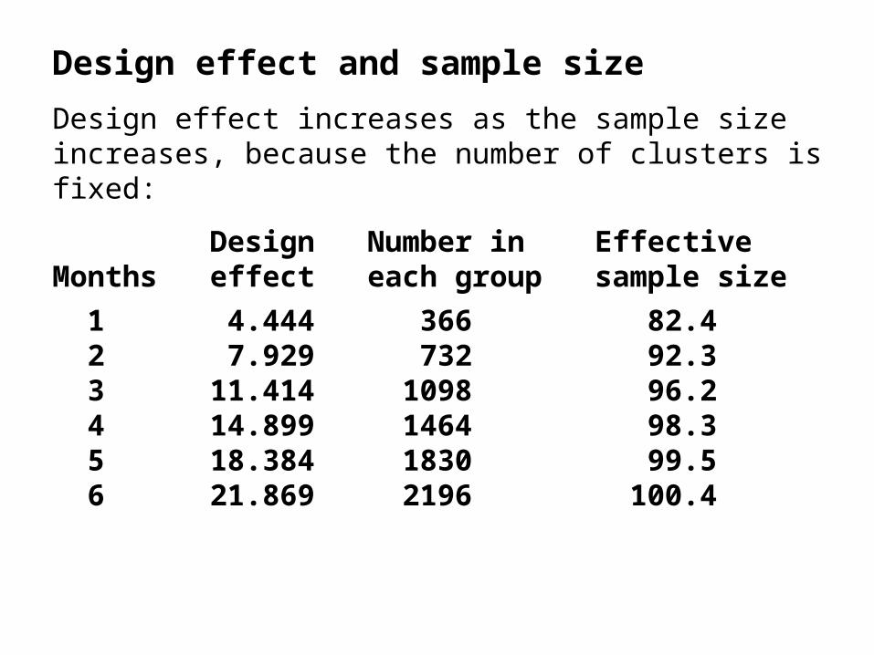
Design effect and sample size

Design effect increases as the sample size increases, because the number of clusters is fixed:

Design Number in EffectiveMonths effect each group sample size

1 4.444 366 82.4 2 7.929 732 92.3 3 11.414 1098 96.2 4 14.899 1464 98.3 5 18.384 1830 99.5 6 21.869 2196 100.4

We need the equivalent of 431 per group.

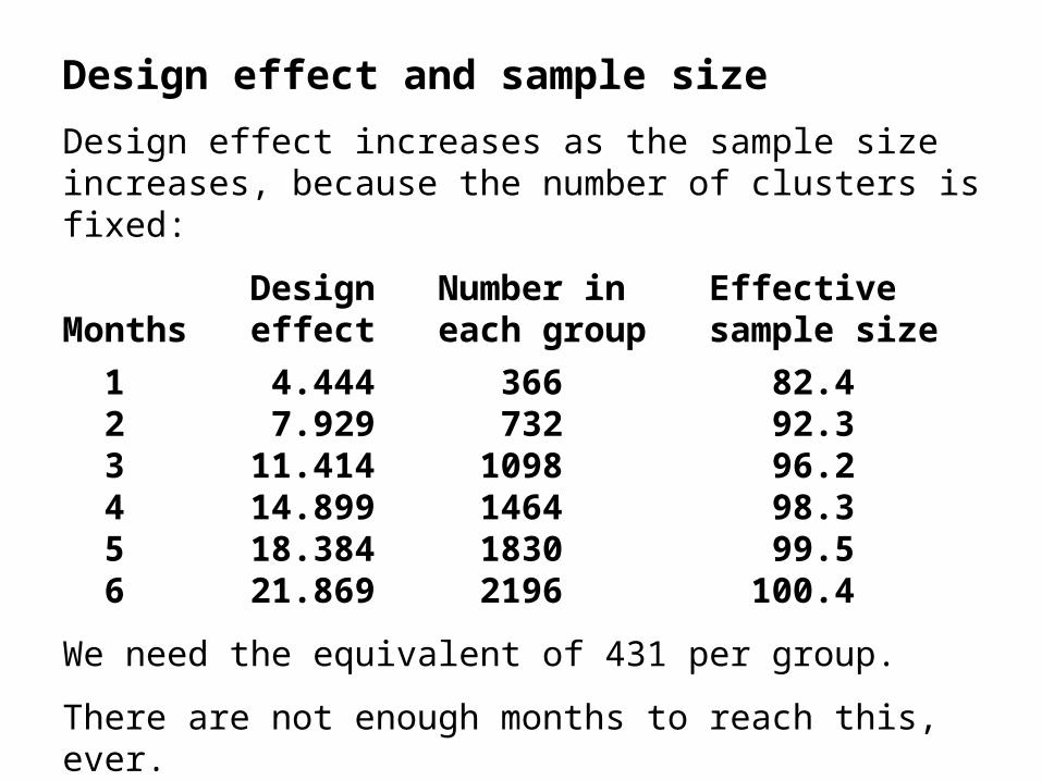
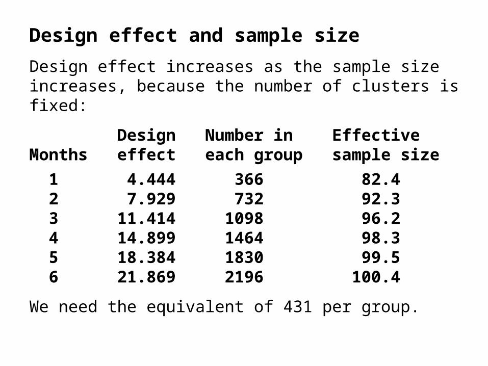
There are not enough months to reach this, ever.

Design effect and sample size

What can we do?

Design effect and sample size

What can we do?

We can get five times the number of hospitals!

Design effect and sample size

What can we do?

We can get five times the number of hospitals!

But there are only 15 available in Scotland and we plan to use 12 in this design.

Design effect and sample size

What can we do?

We can get five times the number of hospitals!

But there are only 15 available in Scotland and we plan to use 12 in this design.

Go to England?

Design effect and sample size

What can we do?

We can get five times the number of hospitals!

But there are only 15 available in Scotland and we plan to use 12 in this design.

Go to England?

‘But, Sir, let me tell you, the noblest prospect which a Scotchman ever sees, is the high road that leads him to England!’ — Dr. Johnson.

Design effect and sample size

What can we do?

We can get five times the number of hospitals!

But there are only 15 available in Scotland and we plan to use 12 in this design.

Go to England?

‘But, Sir, let me tell you, the noblest prospect which a Scotchman ever sees, is the high road that leads him to England!’ — Dr. Johnson.

Make Scotland bigger?

Design effect and sample size

Need to remove the between-hospital variation.

Design effect and sample size

Need to remove the between-hospital variation.

Cannot do a cross-over trial, because midwives cannot unlearn what they have learned.

Design effect and sample size

Need to remove the between-hospital variation.

Cannot do a cross-over trial, because midwives cannot unlearn what they have learned.

Solution: use baseline measurements.

Design effect and sample size

Need to remove the between-hospital variation.

Cannot do a cross-over trial, because midwives cannot unlearn what they have learned.

Solution: use baseline measurements.

Observe the proportion given syntocinon for several months before intervention point and several months after.

Proportions before intervention can be used to remove the inter-hospital variation.

Design effect and sample size

Need to remove the between-hospital variation.

Cannot do a cross-over trial, because midwives cannot unlearn what they have learned.

Solution: use baseline measurements.

Observe the proportion given syntocinon for several months before intervention point and several months after.

Proportions before intervention can be used to remove the inter-hospital variation.

We could use the change in % syntocinon use after intervention point in a two-sample t test.

Design effect and sample size

Need to remove the between-hospital variation.

Cannot do a cross-over trial, because midwives cannot unlearn what they have learned.

Solution: use baseline measurements.

Observe the proportion given syntocinon for several months before intervention point and several months after.

Proportions before intervention can be used to remove the inter-hospital variation.

We could use the change in % syntocinon use after intervention point in a two-sample t test.

It is better to do a covariance analysis on baseline.

Design effect and sample size

Need to remove the between-hospital variation.

Cannot do a cross-over trial, because midwives cannot unlearn what they have learned.

Solution: use baseline measurements.

Observe the proportion given syntocinon for several months before intervention point and several months after.

Proportions before intervention can be used to remove the inter-hospital variation.

We could use the change in % syntocinon use after intervention point in a two-sample t test.

It is better to do a covariance analysis on baseline.

Efficient to use the same number of months before and after.

Design effect and sample size

Need to remove the between-hospital variation.

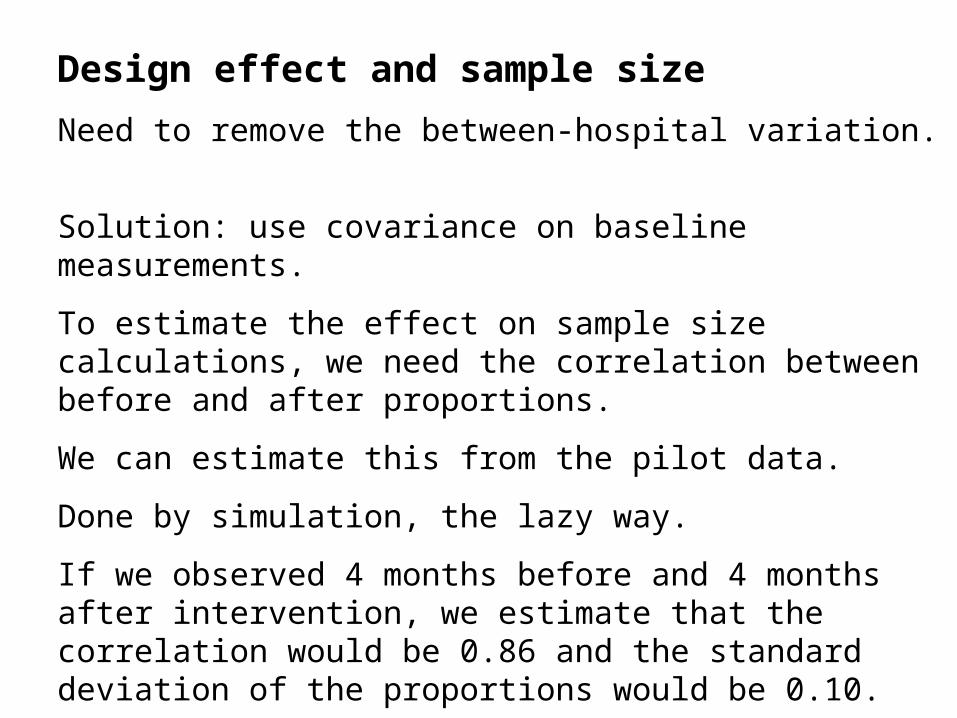
Solution: use covariance on baseline measurements.

To estimate the effect on sample size calculations, we need the correlation between before and after proportions.

Design effect and sample size

Need to remove the between-hospital variation.

Solution: use covariance on baseline measurements.

To estimate the effect on sample size calculations, we need the correlation between before and after proportions.

We can estimate this from the pilot data.

Design effect and sample size

Need to remove the between-hospital variation.

Solution: use covariance on baseline measurements.

To estimate the effect on sample size calculations, we need the correlation between before and after proportions.

We can estimate this from the pilot data.

Done by simulation, the lazy way.

Design effect and sample size

Need to remove the between-hospital variation.

Solution: use covariance on baseline measurements.

To estimate the effect on sample size calculations, we need the correlation between before and after proportions.

We can estimate this from the pilot data.

Done by simulation, the lazy way.

If we observed 4 months before and 4 months after intervention, we estimate that the correlation would be 0.86 and the standard deviation of the proportions would be 0.10.

Design effect and sample size

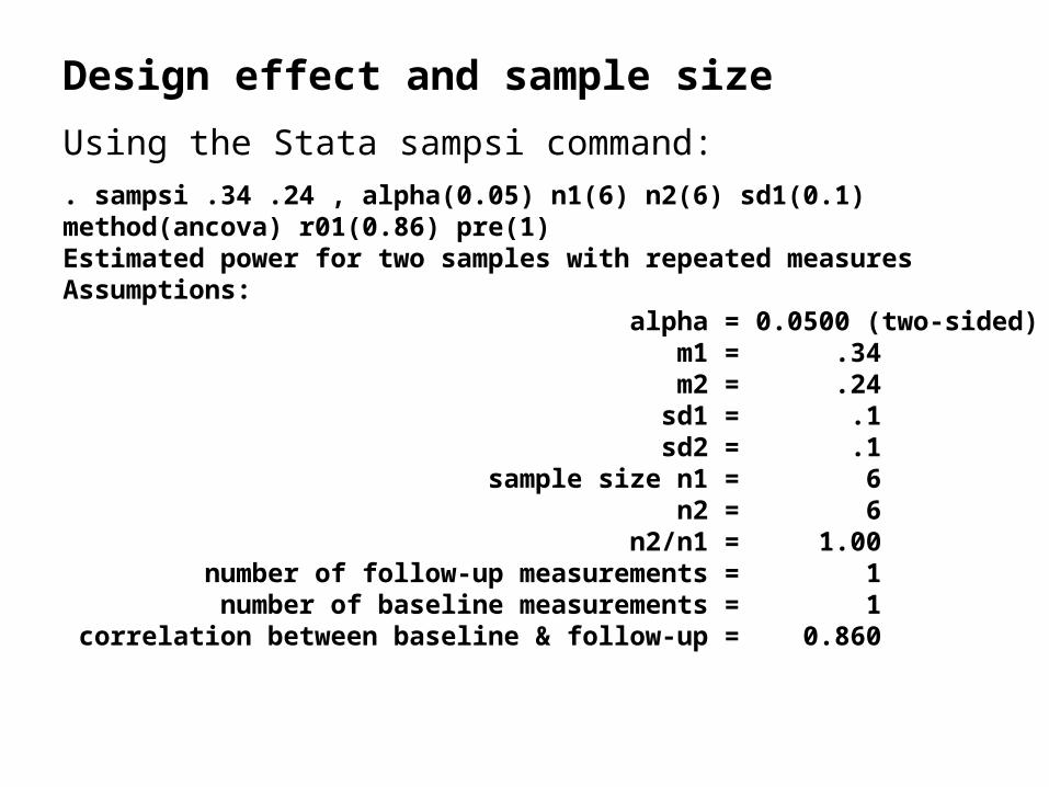
Using the Stata sampsi command:

. sampsi .34 .24 , alpha(0.05) n1(6) n2(6) sd1(0.1) method(ancova) r01(0.86) pre(1)Estimated power for two samples with repeated measuresAssumptions: alpha = 0.0500 (two-sided) m1 = .34 m2 = .24 sd1 = .1 sd2 = .1 sample size n1 = 6 n2 = 6 n2/n1 = 1.00 number of follow-up measurements = 1 number of baseline measurements = 1 correlation between baseline & follow-up = 0.860 

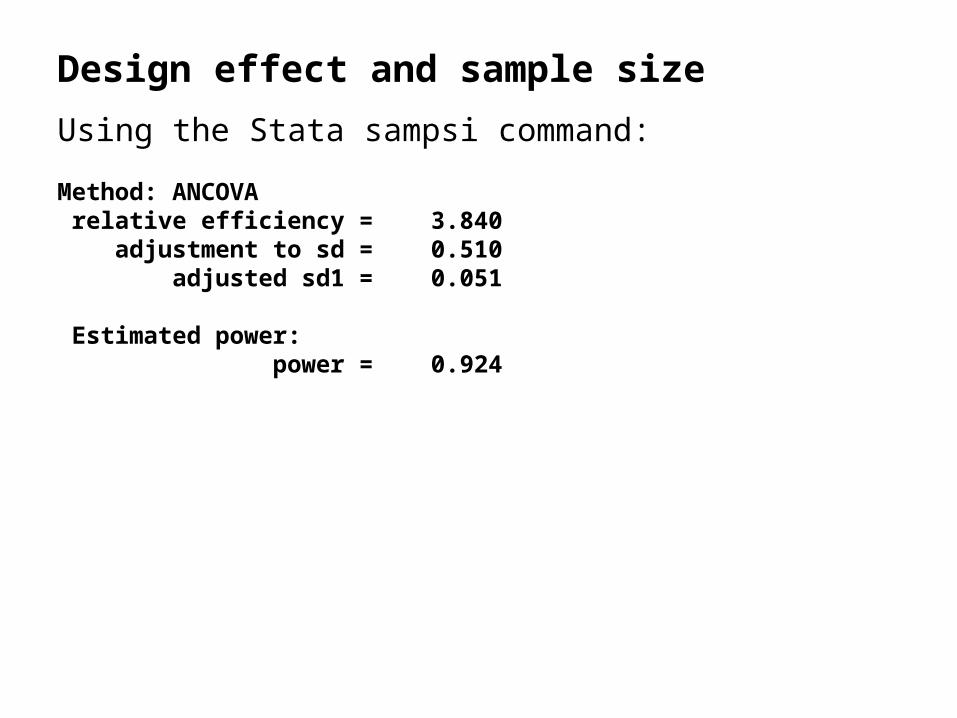
Design effect and sample size

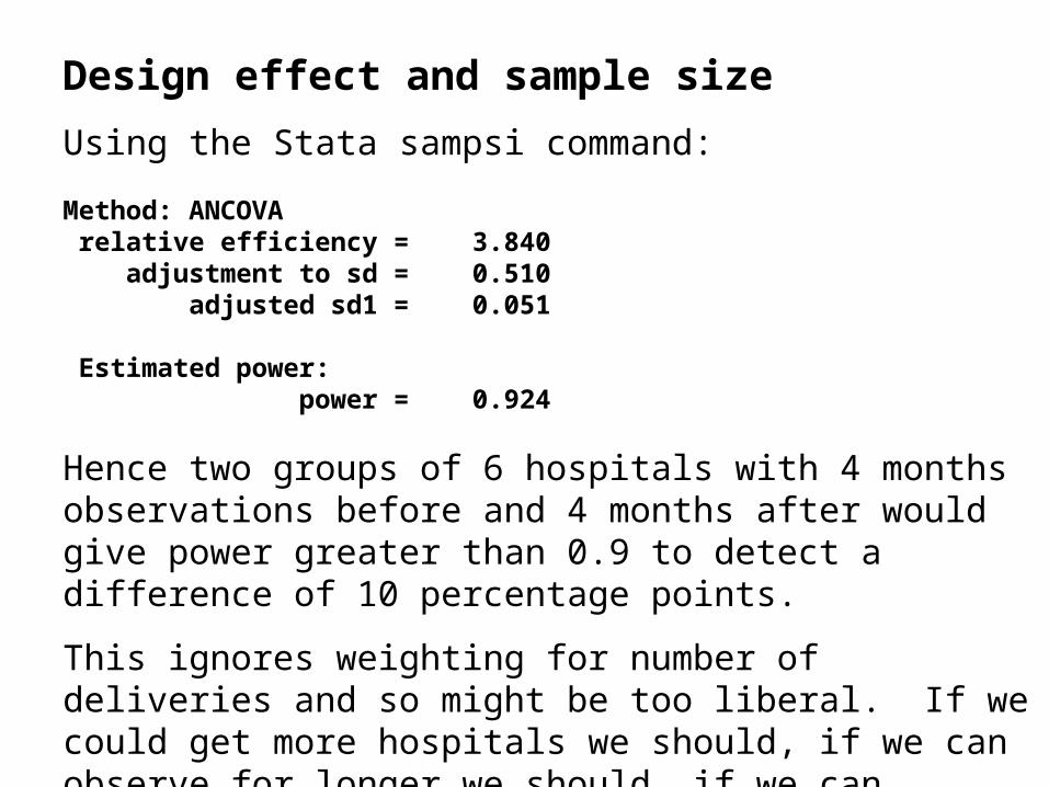
Using the Stata sampsi command: Method: ANCOVA relative efficiency = 3.840 adjustment to sd = 0.510 adjusted sd1 = 0.051  Estimated power: power = 0.924

Design effect and sample size

Using the Stata sampsi command: Method: ANCOVA relative efficiency = 3.840 adjustment to sd = 0.510 adjusted sd1 = 0.051  Estimated power: power = 0.924

Hence two groups of 6 hospitals with 4 months observations before and 4 months after would give power greater than 0.9 to detect a difference of 10 percentage points.

Design effect and sample size

Using the Stata sampsi command: Method: ANCOVA relative efficiency = 3.840 adjustment to sd = 0.510 adjusted sd1 = 0.051  Estimated power: power = 0.924

Hence two groups of 6 hospitals with 4 months observations before and 4 months after would give power greater than 0.9 to detect a difference of 10 percentage points.

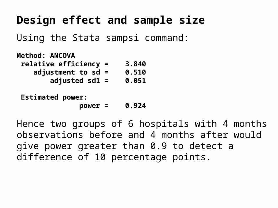
This ignores weighting for number of deliveries and so might be too liberal. If we could get more hospitals we should, if we can observe for longer we should, if we can observe for longer in small units we should. 

Funding

Study funded by the Scottish Executive Health Department.

Funding

Study funded by the Scottish Executive Health Department.

Recruitment

14 hospitals recruited.

Allocated to two groups of 7, using minimisation on presence of midwife birth unit.

Data collection has now begun.

Design of the TELSIS trial

Martin BlandProfessor of Health Statistics

Department of Health SciencesUniversity of York

with Dawn Dowding and Helen Cheyne

www-users.york.ac.uk/~mb55/